Carbon monoxide (CO) cycling in the Fram Strait, Arctic Ocean

Carbon monoxide (CO) influences the radiative budget and oxidative capacity of the atmosphere over the Arctic Ocean, which is a source of atmospheric CO. Yet, oceanic CO cycling is understudied in this area, particularly in light of the ongoing rapid environmental changes. We present results from incubation experiments conducted in the Fram Strait in August–September 2019 under different environmental conditions: while lower pH did not affect CO production (GP_CO) or consumption (k_CO) rates, enhanced GP_CO and k_CO were positively correlated with coloured dissolved organic matter (CDOM) and dissolved nitrate concentrations, respectively, suggesting microbial CO uptake under oligotrophic conditions to be a driving factor for variability in CO surface concentrations. Both production and consumption of CO will likely increase in the future, but it is unknown which process will dominate. Our results will help to improve models predicting future CO concentrations and emissions and their effects on the radiative budget and the oxidative capacity of the Arctic atmosphere.

1 Introduction

Carbon monoxide (CO) is a short-lived atmospheric trace gas which plays an important role in the radiative budget and oxidative capacity of Earth's atmosphere (Forster et al., 2021). Overall, the surface ocean is a minor source of atmospheric CO contributing about 0.4 % to 0.8 % to the natural and anthropogenic sources of CO (Conte et al., 2019; Zheng et al., 2019). However, CO has a comparably short atmospheric lifetime of 1–3 months (Zheng et al., 2019), and thus its oceanic emissions can contribute significantly to the atmospheric CO budget in the atmospheric boundary layer of remote areas such as the Arctic Ocean where the influence of other CO sources is marginal (Blomquist et al., 2012; Kort et al., 2012). However, there are only a few studies on dissolved CO in the Arctic Ocean (Tran et al., 2013; Xie et al., 2009; Xie and Gosselin, 2005). In general the variability in dissolved CO concentrations is higher in the Arctic Ocean as compared to other ocean basins (Tran et al., 2013). Particularly high CO concentrations were measured within bottom sea ice colonized by algae (Xie and Gosselin, 2005; Song et al., 2011).

Oceanic CO is mainly produced photochemically via the reaction of UV light with coloured dissolved organic matter (CDOM) (see e.g. Ossola et al., 2022; Powers and Miller, 2015; Stubbins et al., 2006b; Wilson et al., 1970) and particulate organic matter (POM) (Stubbins et al., 2006a; Song and Xie, 2017). There is also evidence for thermal (dark) CO production from dissolved organic matter (DOM) (Zhang et al., 2008) and for biological CO production by phytoplankton (Tran et al., 2013; Gros et al., 2009; Mcleod et al., 2021). Tran et al. (2013) suggested that Phaeocystis sp.; dinoflagellates; and, to a lesser extent, diatoms are the major biological CO producers in the Fram Strait. However, research on CO production by algae regarding the physiological mechanisms and their interdependencies with biogeochemical parameters is lacking (Campen et al., 2021). Besides the emissions to the atmosphere, microbial consumption is the major loss process of CO in the ocean (Xie et al., 2005; Conrad et al., 1982; Bates et al., 1995).

Ongoing environmental changes in the Arctic Ocean such as the loss of sea ice, changing light penetration in the upper ocean, ocean acidification, and altered nutrient and organic material supply (e.g. Thackeray and Hall, 2019; Stedmon et al., 2011; Hopwood et al., 2018; Terhaar et al., 2020) might affect CO production and consumption pathways as well as emissions to the atmosphere from this region (Campen et al., 2021). The distribution and magnitude of coastal nutrient fluxes is predicted to change (e.g. Hopwood et al., 2018) due to increasing freshwater inputs via ice melting, which could lead to increased stratification and, in turn, limit nutrient availability in the surface layer (Lannuzel et al., 2020). However, between 2012 and 2018 chlorophyll a concentration in Arctic Ocean surface waters increased 16 times faster than before, suggesting an additional input of nutrients that could fuel an increase in primary production (Ardyna and Arrigo, 2020), which in turn might lead to an increase in precursors of CO such as CDOM. Furthermore, light availability and penetration at the ocean surface is projected to increase due to the loss of ice and decreasing albedo (Pistone et al., 2014; Castellani et al., 2022), potentially enhancing CO production in open surface waters and under-ice water during the melting season. Due to the increase in atmospheric carbon dioxide (CO₂), the pH in the surface ocean is decreasing (Canadell et al., 2021), and model projections suggest that pH in Arctic Ocean surface waters could significantly decrease by the end of this century (Terhaar et al., 2020). Decreasing pH (i.e. ocean acidification, OA) is likely to influence the CDOM pool, which, in turn, would alter CO production processes (Hopkins et al., 2020). However, to our knowledge, no studies on the effect of OA on CO cycling in the ocean have been published (Hopkins et al., 2020). How these environmental changes will affect CO production and emissions from the Arctic Ocean is unknown so far due to limited measurements and knowledge gaps with regards to their sources and sinks. To this end, the major objectives of our study were (i) to identify the main drivers of CO production and consumption in the Fram Strait and (ii) to assess the effect of ocean acidification on CO cycling.

2 Materials and methods

2.1 Study area

The study was conducted on board the RRS James Clark Ross during the JR18007 cruise to the Fram Strait from 4 August to 6 September 2019. The Fram Strait, located between the western coast of Svalbard and the eastern coast of Greenland, is characterized by the inflow of Atlantic water via the West Spitsbergen Current (WSC) in the east and Arctic water outflow via the East Greenland Current (EGC) in the west (Rudels et al., 2015). Four incubation experiments were conducted at stations NT6A, Ice2, D7 and D5 (Fig. 1). Stations NT6A, Ice2 and D5 were located at the shelf break, whereas D7 was located in the open-ocean region of the Fram Strait. Moreover, Ice2 and D5 were in proximity to the ice edge. The EGC affected Ice2 as indicated by its lower salinities and colder water temperatures, whereas D5 and D7 were influenced by warmer and more saline Atlantic waters of the WSC (Table S1 in the Supplement).

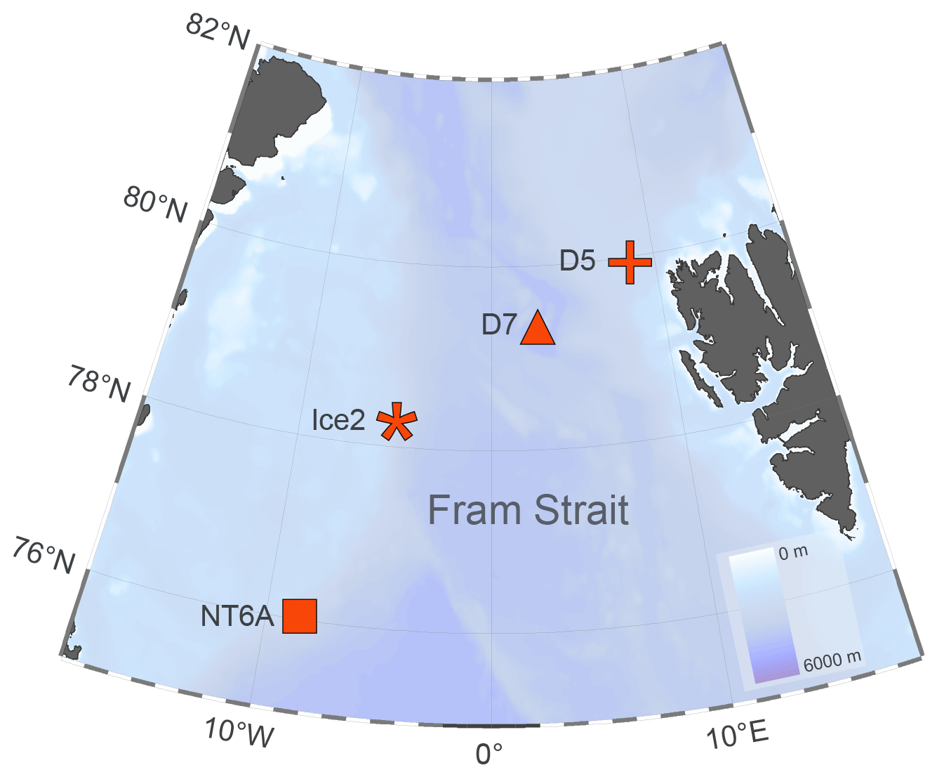
Figure 1 Map showing the locations where incubation experiments were performed (stations NT6A, Ice2, D7 and D5).

2.2 Experimental setup

For the incubation experiments, seawater from 5 m water depth was drawn from Niskin bottles attached to a 12-bottle CTD (conductivity–temperature–depth) instrument/rosette and subsequently incubated in experimental enclosures for up to 48 h. In total, eighteen 3.5 L light-transmitting incubation bottles (DURAN^®, quartz glass, GL 45, DWK Life Sciences, Germany) were filled with seawater. Lids (GL 45) had Teflon-coated septa to easily press out the bulk water and close the bottles in a gas-tight manner. Teflon was chosen to minimize the influence of plastic-derived CO in the experimental setup (Xie et al., 2002). Shading was minimized and natural-light exposure was maximized by placing the bottles upside down in the incubators, which were fixed on a mostly non-shaded area of the ship's deck. To characterize the setting of the upper water, a vertical profile down to 100 m was performed before the start of the incubations. CO concentrations and ancillary measurements (see Sect. S2 in the Supplement) from 5 m water depth served as sampling time 0 (t₀) of the incubations.

Triplicate bubble-free seawater samples for the determination of dissolved CO were taken in 100 mL glass vials (both from Niskin bottles and incubation bottles) by using a Tygon^® tubing to avoid contamination by silicone rubber (Xie et al., 2002). The vials were immediately sealed with Teflon-coated stoppers to minimize CO contamination (Xie et al., 2002). The vials were stored between 0 and 6 ^∘C in the dark to suppress further CO photoproduction. CDOM was sampled in brown 500 mL glass vials with a screwed cap. Inorganic nitrate samples were drawn into 10 mL polyethylene tubes, which were pre-rinsed three times with sample water and stored at −80 ^∘C until analysis at GEOMAR's Chemical Oceanography department. CDOM samples were stored in the dark and below 5 ^∘C until filtration (for details on the method, see Sect. S2).

The pH in each experiment was manipulated to represent three different atmospheric CO₂ mole fractions: 405.43 ± 0.05 (Dlugokencky et al., 2021), 670 and 936 ppm CO₂ for the treatments named ambient, pH1 and pH2, respectively. To this end, the pH in pH1 and pH2 was adjusted by lowering the pH by 0.14 and 0.3, respectively, to approximate that of the IPCC's (Intergovernmental Panel on Climate Change) RCP4.5 (Representative Concentration Pathway; moderate change) and RCP8.5 (extreme change) relative to the ambient carbonate chemistry of the seawater at the time of the sampling (Table S2 in the Supplement). To manipulate the carbonate system, NaHCO₃ and HCl were added (Riebesell et al., 2011) and checked for the resulting total alkalinity (TA) and dissolved inorganic carbon (DIC) concentrations (Table S2). Values of pCO₂ and pH_T (total scale) were calculated with the software programme CO2sys (Lewis and Wallace, 1998). Immediately after pH manipulation, bottles were closed in a gas-tight manner and incubated.

Light incubators had transparent Plexiglas^® sidewalls (GS 2458, UV transmitting) and no lid so that the full natural sunlight spectrum could penetrate the enclosed incubation bottles from the sides and above (self-manufactured according to experimental needs; Fig. S3.1 in the Supplement). While these incubators were placed on deck to allow for natural sunlight penetration, black and covered water chambers served as dark incubators to exclude any light. The incubation bottles were placed inside the incubators which were filled with ambient seawater pumped through the incubator to keep bottles at ambient-seawater temperatures. Light and temperature were monitored continuously in each incubator (temperature/light, onset, HOBO Pendant^®, USA). Oxygen saturation (in %) was monitored to make sure that the incubations did not become anoxic (O2xyDot^®, OxySense, USA). CO concentrations were determined at the beginning of the incubation (t₀), after 12 (t₁₂), 24 (t₂₄) and 48 h (t₄₈) of incubation (Fig. S3.1).

2.3 CO measurements

Dissolved CO concentrations were determined by the headspace method as described by Xie et al. (2002). We established a headspace by injecting 15 mL of CO-free synthetic air (purified via MicroTorr series, 906 Media, SAES Getters, USA). The samples were then equilibrated for 8 min (Law et al., 2002; Xiaolan et al., 2010). A 5 mL subsample from the equilibrated headspace was injected with a gastight syringe into the sample loop of a CO analyser (ta3000, AMETEK, USA). Every sixth sample injection was followed by the injection of a standard gas mixture with 113.9 ppb CO in synthetic air (Deuste Gas Solutions, Germany) which was calibrated against a certified standard gas (250.5 ppb CO, calibrated against the NOAA 2004 scale at the Max Planck Institute for Biogeochemistry, Jena, Germany). This value was chosen as it lies in the expected range of the CO mole fraction equilibrated with open-ocean waters. Blank measurements were performed before sample measurements by injecting CO-free synthetic air. No contamination by CO was detectable, and, therefore, no blank correction was applied.

Measured CO mole fractions from the headspace were corrected for the drift of the detector with the standard gas measurements and corrected for water vapour (Wiesenburg and Guinasso, 1979). The final dissolved CO concentrations were calculated based on Stubbins et al. (2006) with the solubility coefficients from Wiesenburg and Guinasso (1979). For each of the CO concentration triplicates we calculated the arithmetic mean and estimated the standard error according to David (1951). The overall mean error for the measurements of dissolved CO was ±0.025 nmol L⁻¹ (±17.4 %). The lower detection limit of the CO analyser is 10 ppb CO in air, which translates to a detection limit of about 0.01 nmol L⁻¹ for dissolved CO concentrations at equilibrium at water temperatures of −1 to 4 ^∘C and salinities of 30 to 35.

2.4 CO consumption and production rates

Net CO consumption (NC_CO) and net production rates (NP_CO) were calculated as the slope of the linear regression line for CO concentration [CO] loss and increase over the duration of the experiment (48 h) and per pH treatment:

$$\begin{array}{}\text{(1)}& {\displaystyle }{\text{NC}}_{\mathrm{CO}}=-\left[\mathrm{CO}\right]\cdot t^{-\mathrm{1}},\text{(2)}& {\displaystyle }{\text{NP}}_{\mathrm{CO}}=\left[\mathrm{CO}\right]\cdot t^{-\mathrm{1}}.\end{array}$$

Gross production rates of CO (GP_CO) were calculated as the sum of NP_CO and the absolute value of NC_CO in order to demask the effect of microbial CO consumption in the light experiments:

$$\begin{array}{}\text{(3)}& {\text{GP}}_{\mathrm{CO}}={\text{NP}}_{\mathrm{CO}}+{\text{NC}}_{\mathrm{CO}}.\end{array}$$

To increase data points when possible, single CO gross production rates (singleGP_CO) were calculated between two sampling times (0–12, 0–24, 0–48 h) for each treatment and for each experiment, respectively. Since consumption rates followed a first-order loss for all experiments (Figs. 2 and S3.2 in the Supplement), the consumption rate constant (k_CO) for each experiment was determined as the slope of the respective linear regression.

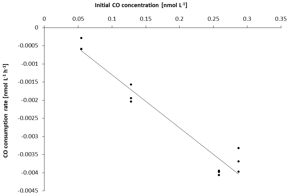
Figure 2 Initial CO concentrations plotted against overall consumption rates per experiment. All consumption rates depend on the initial CO concentration (i.e. first-order loss; R²=0.94 with p<0.05; see also Fig. S3.2).

3 Results and discussion

3.1 CO concentration development during dark and light incubations

The low initial CO concentrations (Table 1) are in line with the observation that CO in surface waters can show a pronounced seasonal variability in Arctic waters. For example, Xie et al. (2009) reported considerably lower CO concentrations for September–October 2003 (0.17–1.34 nmol L⁻¹) than for June 2004 (0.98–13 nmol L⁻¹) in the Amundsen Gulf (Beaufort Sea). Tran et al. (2013) reported a mean CO concentration of 6.5 ± 3.2 nmol L⁻¹ in polar waters of the Fram Strait in July 2010. And only recently Gros et al. (2023) reported mean CO concentrations in the range from 1.5 ± 1.7 (in surface waters at sea-ice stations) to 5.9 ± 2.9 nmol L⁻¹ (in polar waters) from the Fram Strait in May–June 2015.

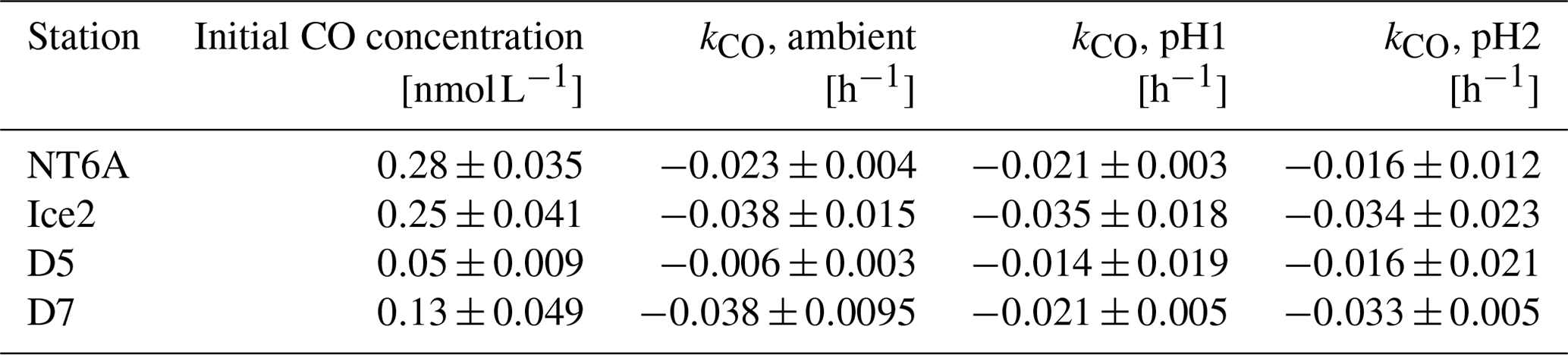
Table 1 Initial CO concentrations and CO consumption rate constants (k_CO) of the four incubation experiments conducted at different pH levels. Data are given as the mean ± the estimate of the standard deviation (for the initial CO concentrations) and as the slope of the linear regression ± the error in the slope (for k_co).

CO concentrations decreased with time in all dark incubations, with the exception of pH2 at NT6A (Figs. 3 and S3.2). While the general decrease in CO was most likely driven by microbial consumption, which is the major known CO consumption process in Arctic waters (e.g. Xie et al., 2005, 2009), elevated CO concentrations at NT6A (pH2) could hint towards ongoing thermal CO production (Zhang et al., 2008). All light treatments showed a diurnal pattern of light intensity, though light was never completely absent because the incubations were performed in the Arctic summer. CO concentrations in the light incubations showed no uniform trend with time. Only during the incubations of NT6A and D5 was a significant increase in CO concentrations over 48 h observed. However, this a net production which includes microbial CO consumption. Since there was no obvious relationship between the timing of the sampling, CO concentrations and preceding light intensities (Fig. 3), this indicates that photochemical CO production did not exceed CO consumption. We therefore suggest that if there was photochemical CO production, it was directly consumed by bacteria. Alternatively, biological CO production by phytoplankton (Gros et al., 2009; Tran et al., 2013) or bacterioplankton and/or thermal production might have been dominant at NT6A and D5 (Zhang et al., 2008).

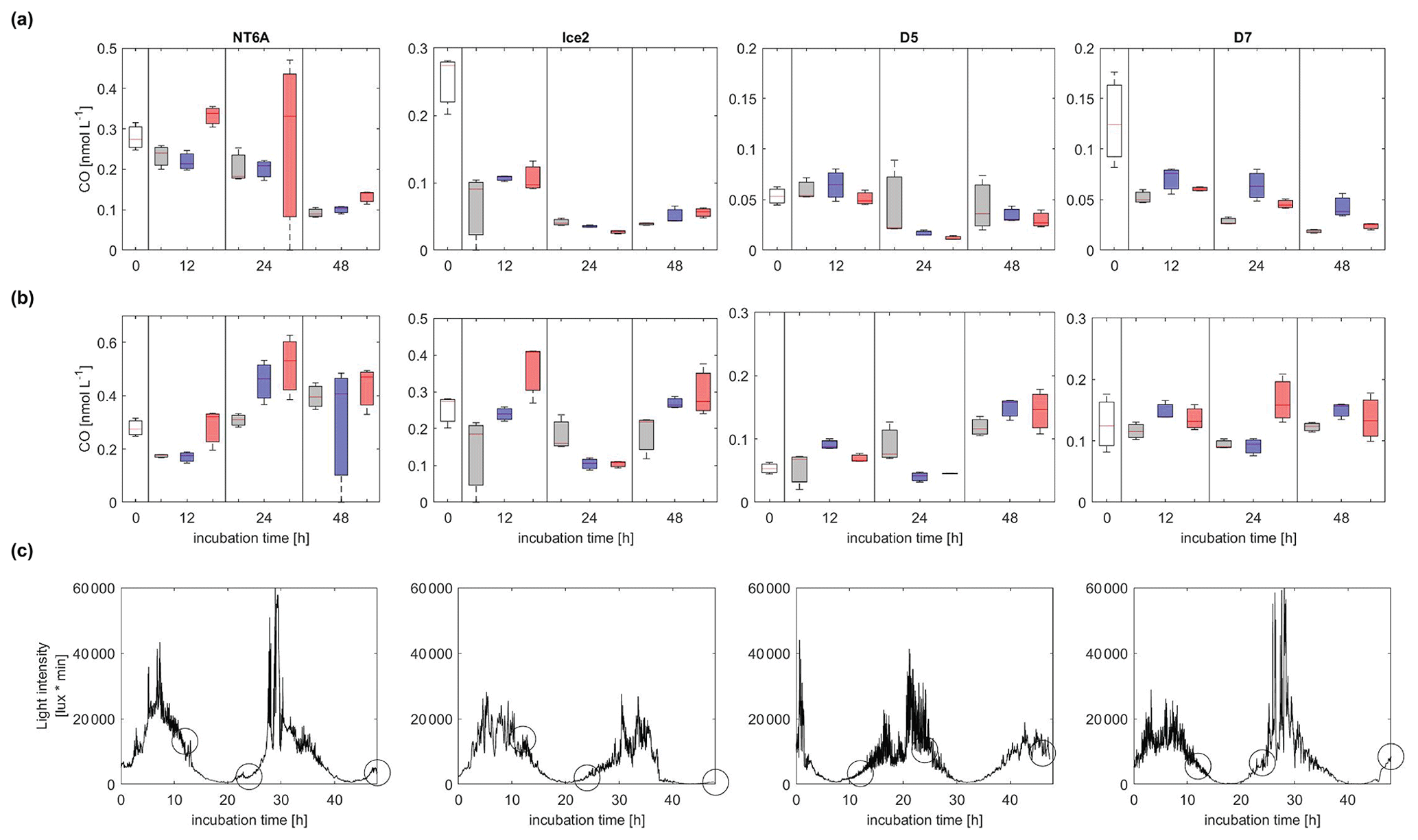
Figure 3 Development of CO concentrations (nmol L⁻¹) over 48 h of incubations (a) in the dark and (b) in natural sunlight. Panel (c) shows the respective light intensities in the light treatments at each station (light intensities in the dark treatment were zero). Circles indicate the timing of sampling events in dark and light treatments; white: initial concentration, grey: ambient, blue: pH1, red: pH2. The station names are indicated on the top. Please note that the scales of the y axes vary between stations according to their CO maximum concentrations. The vertical extent of the bars in (a) and (b) depicts the spread of triplicate samples, and the line within each bar indicates the average.

The k_CO data computed from our experiments (Table 1) are comparable to previously published findings from Arctic waters: Xie et al. (2005) reported first-order consumption rates constants k_CO of −0.040 ± −0.012 and −0.020 ± −0.0060 h⁻¹ in the coastal and offshore Beaufort Sea, respectively. (Please note that k_CO values are given as positive values in Xie et al., 2005).

In general, a lower pH did not affect the CO concentrations in the dark incubations or in the light incubations, since the CO concentrations in the pH-manipulated treatments did not differ significantly from the ambient treatments (as indicated by the error bars in Fig. 3). Accordingly, pH affected neither k_CO nor GP_CO significantly during our incubations (see also Fig. S3.3 in the Supplement).

3.2 Effect of environmental variability on CO consumption and production

We observed contrasting hydrographic settings at the stations selected or in the incubation experiments. While Ice2 was located close to the ice edge and had a low water temperature and low salinity at t₀, D7 was located in the open Fram Strait with a higher water temperature and salinity at t₀ (Fig. 4). Therefore, Ice2 was most probably affected by freshwater input from ice melting and polar waters carried by the EGC (Fig. 4 and Table 1). D5 had a lower salinity compared to D7 and was also (at least partly) affected by freshwater from ice melting. NT6A had a low salinity which was comparable to Ice2, but the water temperature at t₀ was much higher compared to Ice2. Moreover, station NT6A had a steep halocline at about 10 m, whereas Ice2 was well mixed in the upper layer (Fig. S3.4). Therefore, NT6A also being the southernmost station during our study had an apparently different hydrographic setting in comparison to the other three stations. When considering all stations except for NT6A, GP_CO showed a statistically significant correlation (R²=0.58, p<0.05) with increasing density. This suggests that surface waters in the Fram Strait with a higher fraction of freshwater (i.e. lower density), due to e.g. fresh meltwater or polar inflow in the western Fram Strait, potentially lead to higher CO production rates. There was no significant relationship for k_CO with density, which indicates that, besides meltwater and polar waters, additional factors must have influenced CO consumption in the area at the time of sampling.

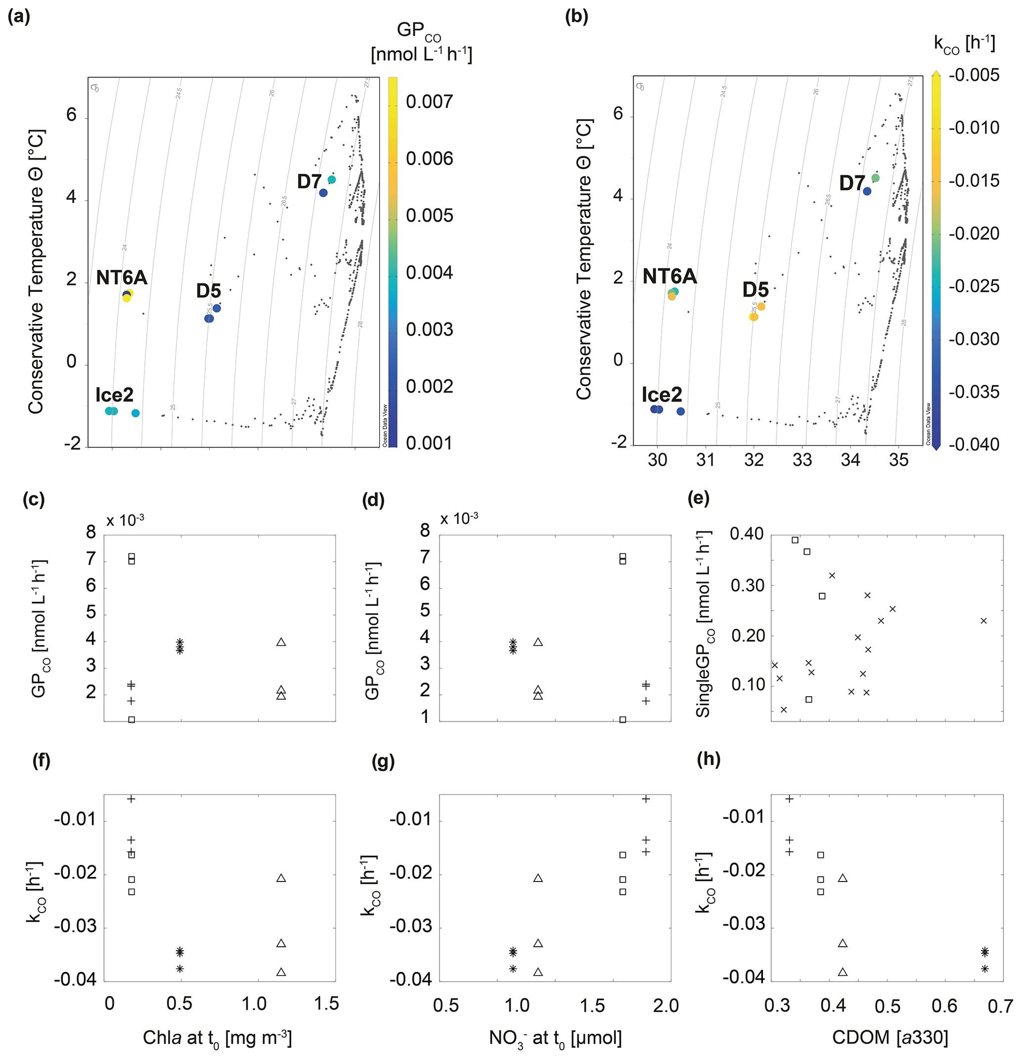
Figure 4 Relationship between GP_CO, k_CO and selected environmental variables during the study. (a) Temperature–salinity plot including GP_CO, (b) temperature–salinity plot including k_CO, (c, d) GP_CO vs. chl a and ${{\mathrm{NO}}_{\mathrm{3}}}^{-}$ at t₀, (e) singleGP_CO vs. CDOM absorption (330 nm) at each sampling time, (f–h) k_CO vs. chl a and ${{\mathrm{NO}}_{\mathrm{3}}}^{-}$ and CDOM absorption (330 nm) at t₀. □: NT6A, *: Ice2, +: D5, Δ: D7, ×: CDOM values at single sampling times of all stations excluding NT6A. In (a) and (b) isolines represent density.

Given that CDOM is the major driver for CO photoproduction in the ocean (see e.g. Ossola et al., 2022), a good correlation between both was an underlying assumption during our experiments. We observed that CDOM absorption for all treatments significantly correlated with singleGP_CO (R²=0.45, p<0.05, Fig. 4; data from NT6A excluded). Moreover, CDOM absorption at t₀ was significantly correlated with k_CO (R²=0.57, p<0.05). Given that photochemical production from CDOM is a CO source, this is most likely an indirect correlation: high CDOM absorption induces photochemical CO production which, in turn, results in higher CO consumption (i.e. a lower k_CO) because k_CO depends on the initial CO concentration.

Neither GP_CO nor k_CO was significantly correlated with chl a concentrations during our experiments (Fig. 4). This is in contrast to Xie et al. (2005), who reported a negative correlation between chl a and k_CO (please note again that Xie et al., 2005, reported k_CO as positive values). This suggests that $\text{chl}a/k_{\mathrm{CO}}$ relationships seem to be variable within the Arctic realm, possibly as a result of the complex interplay between different water masses (Cherkasheva et al., 2014; Rudels et al., 2015). Nitrate (${{\mathrm{NO}}_{\mathrm{3}}}^{-}$) concentrations at t₀ and GP_CO were negatively correlated (albeit statistically not significant at the 95 % significance level and after excluding NT6A data; Fig. 4), while k_CO was positively correlated with ${{\mathrm{NO}}_{\mathrm{3}}}^{-}$ concentrations at t₀ (R²=0.78, p<0.05, Fig. 4). The combination of relatively higher chl a concentrations at t₀ and lower ${{\mathrm{NO}}_{\mathrm{3}}}^{-}$ concentrations at Ice2 and D7 with respect to NTA6 and D5 could explain the higher CO consumption rates at the two stations: on the one hand, CO is known to act as competitive inhibitor for ammonium monooxygenase (amoA; the enzyme responsible for ammonium oxidation during nitrification; Zhang et al., 2020), resulting in cell uptake of CO under nutrient-deprived conditions (see Vanzella et al., 1989) as those found at the time of sampling. On the other hand, field and laboratory studies (Moran and Miller, 2007, and references therein; Cordero et al., 2019) have shown the ability of bacterioplankton (e.g. the Roseobacter clade) to oxidize CO during heterotrophic growth (i.e. using it as a supplementary energy source rather than a fixed carbon source for building biomass), in particular under oligotrophic conditions. The fact that we still measured oxidation rates in waters with very low CO concentrations might indicate that the dominant community is rather heterotrophic, which in turn could help in explaining the poor correlation with chl a. This finding is important for modelling studies constraining marine CO sources and sinks in the framework of future scenarios where warming-derived stratification reduces ${{\mathrm{NO}}_{\mathrm{3}}}^{-}$ supply to the surface ocean. Under such “starvation” conditions, inorganic compounds such as CO could help in sustaining small planktonic communities.

Recent results show that ${{\mathrm{NO}}_{\mathrm{3}}}^{-}$ can enhance the photoproduction of carbonyl sulfide (OCS) (Li et al., 2022). OCS and CO photoproduction have a common intermediate in their photoproduction pathways, but photoproduction of OCS and CO in natural waters is anticorrelated (Pos et al., 1998). Even though it is based on indirect evidence, we suggest that the trend of decreasing CO photoproduction (GP_CO) with increasing ${{\mathrm{NO}}_{\mathrm{3}}}^{-}$ concentrations might be caused by the mechanism suggested by Pos et al. (1998).

4 Conclusions

In order to decipher the cycling of CO in the surface waters of the Fram Strait, we measured CO production and consumption rates in various incubation experiments at four sites in the Fram Strait in summer 2019. We conclude that ocean acidification may not affect CO gross production (GP_CO) and consumption (k_CO) rates. Thus, CO produced in surface waters could be rapidly consumed before being emitted to the atmosphere. In consequence, CO production at these depths does not necessarily result in outgassing towards the atmosphere. We therefore infer that CO consumption mainly drives dissolved CO concentrations and hence could act as a “filter” for the subsequent atmospheric CO emissions from the Fram Strait. High rates of both CO production and CO consumption were favoured by a combination of high CDOM and low ${{\mathrm{NO}}_{\mathrm{3}}}^{-}$ concentrations. This suggests a photochemical production of CO from CDOM, which, in turn, is consumed rapidly by microbes preferably under oligotrophic conditions such as those found at the time of sampling. In the Arctic Ocean and Fram Strait, such conditions can be found, at least transiently, both at ice edges as well as in the open ocean, where a supply of nutrients via melting and/or mixing is followed by stratification (Cherkasheva et al., 2014). We identified both CDOM and ${{\mathrm{NO}}_{\mathrm{3}}}^{-}$ as key drivers of CO cycling. This has the implication that predicted changes in terrestrially derived and marine CDOM (e.g. Lannuzel et al., 2020), as well as dissolved ${{\mathrm{NO}}_{\mathrm{3}}}^{-}$ inputs (Tuerena et al., 2022), could affect future CO production and consumption in the region. Both trends might lead to higher CO gross production as well as higher CO consumption. It is yet uncertain whether both terms will balance each other out or whether one process will become dominant. The question of if and under which conditions CO consumption rates would stagnate should be addressed in future research, since in that situation CO would actually be emitted. Performing further multifactorial experiments including e.g. UV light intensity and bacterial community data could help to elucidate the explanatory power of the different environmental factors on both CO production and consumption. This would facilitate a better incorporation of both terms into biogeochemical models and would improve both CO emission estimates for the Arctic realm and the assessment of how atmospheric CO emissions will affect the radiative budget and oxidative capacity of the Arctic atmosphere.