the Creative Commons Attribution 4.0 License.
the Creative Commons Attribution 4.0 License.
 | 11 Jan 2023
Phytoplankton reaction to an intense storm in the north-western Mediterranean Sea
Stéphanie Barrillon
Robin Fuchs
Anne A. Petrenko
Caroline Comby
Anthony Bosse
Christophe Yohia
Jean-Luc Fuda
Nagib Bhairy
Frédéric Cyr
Andrea M. Doglioli
Gérald Grégori
Roxane Tzortzis
Francesco d'Ovidio
Melilotus Thyssen
The study of extreme weather events and their impact on ocean physics and biogeochemistry is challenging due to the difficulty involved with collecting in situ data. However, recent research has pointed out the major influence of such physical forcing events on microbiological organisms. Moreover, the occurrence of such intense events may increase in the future in the context of global change. In May 2019, an intense storm occurred in the Ligurian Sea (north-western Mediterranean Sea) and was captured during the FUMSECK (Facilities for Updating the Mediterranean Submesoscale – Ecosystem Coupling Knowledge) cruise. In situ multi-platform (vessel-mounted acoustic Doppler current profiler, thermosalinometer, fluorometer, flow cytometer, a moving vessel profiler equipped with a multi-sensor towed vehicle, and a glider) measurements along with satellite data and a 3D atmospheric model were used to characterise the fine-scale dynamics occurring in the impacted oceanic zone. The most affected area was marked by a lower water temperature (1 ∘C colder), a factor of 2 increase in surface chlorophyll a, and a factor of 7 increase in the nitrate concentration, exhibiting strong gradients with respect to the surrounding waters. Our results show that this storm led to a deepening of the mixed-layer depth from 15 to 50 m and a dilution of the deep chlorophyll maximum. As a result, the surface biomass of most phytoplankton groups identified by automated flow cytometry increased by up to a factor of 2. Conversely, the carbon / chlorophyll ratio of most phytoplankton groups decreased by a factor of 2, evidencing significant changes in the phytoplankton cell composition. These results suggest that the role of storms on the biogeochemistry and ecology of the Mediterranean Sea may be underestimated and highlight the need for high-resolution measurements during these events coupling physics and biology.
- Article
(6719 KB) - Full-text XML
- BibTeX
- EndNote


Marine environments are subject to short-term events whose effects on biogeochemical processes can be substantial. This is the case for desert dust deposition on oligotrophic areas (Guieu et al., 2014), volcanic ash deposition (Hamme et al., 2010), submarine sources of iron (Guieu et al., 2018), and sudden mixing of the water column due to typhoons (Wang, 2020). Even the classic phytoplankton spring bloom can vary in intensity and spatial extent depending on the number of previous short-term storms (Ferreira et al., 2022). The effects of these processes on marine micro-organisms, such as phytoplankton, include sudden changes in diversity and abundance. Depending on the redistribution of nutrients, the turbulence, the light conditions, and the mixing of different water masses, the phytoplankton community can collapse or grow, affecting carbon export by generating decoupling phenomena between production and remineralisation (Henson et al., 2019).
Meteorological impulse wind events, such as storms, and their effects on oceanic physics and biogeochemistry are poorly explored with in situ data. Such events generate mixing and stirring of the surface layer and can trigger transitional peaks in primary production, mainly explained by nitracline shoaling and grazer dilution (Lomas et al., 2009; Menkes et al., 2016). Under oligotrophic ocean conditions, Babin et al. (2004) and Han et al. (2012) observed sudden and large increases in chlorophyll a (Chl a) from satellite ocean colour data that lasted for several weeks after summer hurricane storms. The resulting increase in Chl a integrated over the first few metres reached values close to those of the spring bloom (Babin et al., 2004) with potential primary production comparable to that induced by some mesoscale (∼ 10–100 km horizontal range) eddies. Nevertheless, the authors were limited in their interpretation due to the lack of in situ observations. Only a few studies have combined high-resolution physical descriptions of wind events with a phytoplankton resolution at the functional group level. Some coastal studies, such as Fuchs et al. (2023), have evidenced pico- and nanophytoplankton abundance and biomass responses (positive for most phytoplankton groups) within 2–4 d following wind-induced events under stratified conditions at a coastal station located in the north-western (NW) Mediterranean Sea. The authors showed that extreme events can generate daily biomass increases of the same order of magnitude as those observed during the spring bloom. Similarly, Anglès et al. (2015) studied the response of nano- and microphytoplankton (>10 to ∼ 150 µm) to tropical cyclones generating wind-related physical forcing and substantial rains in the western Gulf of Mexico. They highlighted strong increases in plankton abundance following the storms, with delays consistent with Fuchs et al. (2023). These storms, which were observed in either coastal Mediterranean systems or tropical open ocean regions, may also exert a strong control on both primary production and community structure in the Mediterranean open ocean, thereby playing a potentially important biogeochemical role in the whole basin. However, to our knowledge, no such event has been reported in the Mediterranean open ocean in the past.
The classic spring bloom as observed in temperate oceans is triggered by the shoaling of the mixed layer during the transition from winter convection to spring stratification (Behrenfeld, 2010). The bloom ends when no more nutrients are available in the euphotic layer or when grazers surpass the phytoplankton growth capacity. This is particularly the case in the NW Mediterranean Sea, which is characterised by winter deep convection (Houpert et al., 2016; Testor et al., 2018) and by spring blooms of different intensities that can be detected from satellite images (d'Ortenzio and Ribera d'Alcalà, 2009; Mayot et al., 2016). This area is affected by strong northerly winds, and the strength of these winds in winter defines the bloom intensity (Conan et al., 2018). Under summer stratified conditions, impulse wind events could induce submesoscale (∼ 1–10 km horizontal range) vertical mixing and trigger patches of high phytoplankton production. However, observing the effect of these events on the phytoplankton dynamics and distribution is challenging, especially under stratified oligotrophic conditions, and requires the deployment of dedicated automated and high-frequency sampling tools. Indeed, the mixing of the water column may bring microorganisms from the deep to surface layers, affect their physiological properties due to photoacclimation processes, and impact their carbon / chlorophyll ratios, which are used to run primary production models at large scales (Sathyendranath et al., 2020). In addition, some scarce observations at the functional group level evidence daily adaptation processes rather than community changes after water column mixing (Thompson et al., 2018) or a taxonomical dependency on physiological strategies (Graff and Behrenfeld, 2018). Being able to monitor the phytoplankton distribution at a functional level, by integrating small- and rapid-scale dynamics into larger space and time, would more precisely elucidate the role of phytoplankton in biogeochemical processes.
The objective of this paper is to study the in situ physical and biological effects of a particularly intense wind episode that occurred in spring 2019 in the Ligurian Sea (NW Mediterranean Sea) during the FUMSECK (Facilities for Updating the Mediterranean Submesoscale – Ecosystem Coupling Knowledge) cruise (https://doi.org/10.17600/18001155; Barrillon et al., 2020). High-resolution physical properties of the water column and the surface phytoplankton functional group distribution were combined to show abrupt changes in water characteristics, surface phytoplankton abundances, and physiological indicators.
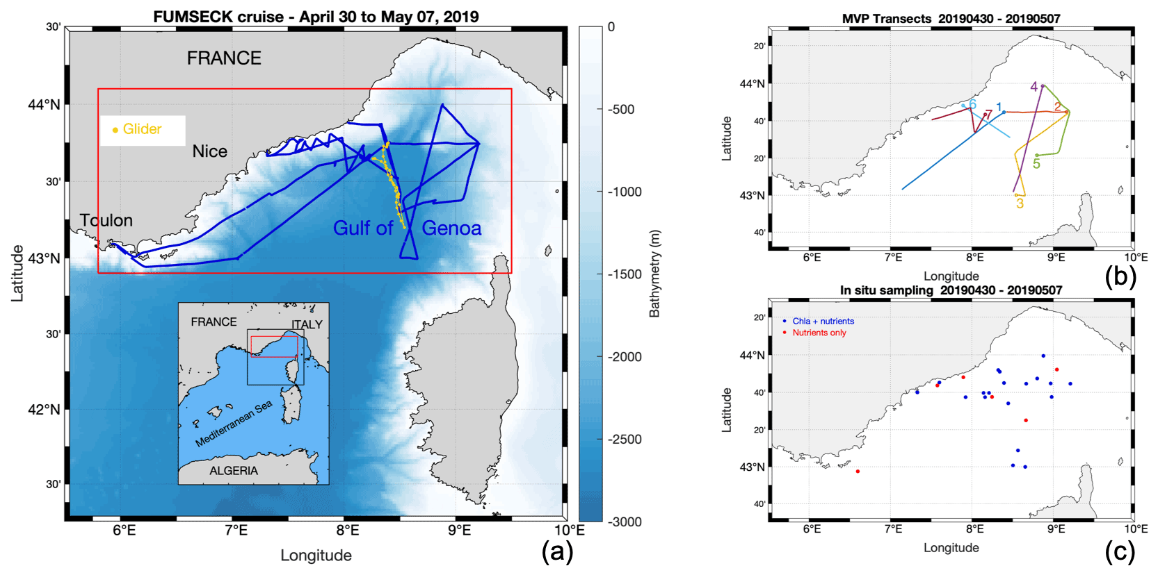
Figure 1Panel (a) presents the FUMSECK cruise (blue line), superimposed with bathymetry. The geographical domain is represented in red, and the glider trajectory is shown in yellow. Panel (b) shows the MVP transects, numbered from 1 to 7 at the end of the transects. Panel (c) outlines the in situ sampling of Chl a and nutrients.
The FUMSECK cruise aimed at simultaneously sampling physical and biogeochemical data for the study of mesoscale and submesoscale dynamics, which imply structures such as eddies, filaments, or fronts over a horizontal spatial range of 1 to 100 km, a vertical range of 0.1 to 1 km, and a temporal range of days to a few weeks (Giordani et al., 2006; Ferrari and Wunsch, 2009; McWilliams, 2019). It took place from 30 April 2019 to 7 May 2019 in the Ligurian Sea (NW Mediterranean Sea) aboard the RV Téthys II. The circulation in the Ligurian Sea is generally cyclonic and characterised by a strong westward-flowing geostrophic current along the coastline (Esposito and Manzella, 1982). The Northern Current (Millot, 1999), hereafter called “NC”, corresponds to the northern branch of the current along the coastline. During this cruise, we deployed towed instruments (a moving vessel profiler, MVP) and an underwater glider (Testor et al., 2019) to measure physical properties at high resolution. These measurements have been paired with shipboard measurements of phytoplankton functional groups from an automated pulse-shape recording flow cytometer, based on cell sizes and pigment contents (Dugenne et al., 2014; Thyssen et al., 2014; Bonato et al., 2015; Louchart et al., 2020). Figure 1 shows the cruise and the glider trajectories, the MVP transects, and the positions of the surface discrete sampling locations for nutrients and Chl a. A storm hit the region between 4 and 5 May. Right after the storm, during which we had to take shelter, the ship returned to the wind-exposed zone to collect data. The glider, in contrast, remained in the storm-exposed zone throughout the storm period and collected data. In addition to in situ data, we exploited satellite data, to guide the cruise and obtain a synoptic view of the region, and a meteorological model to study the storm.
2.1 Transect measurements
The vessel-mounted acoustic Doppler current profiler (VM-ADCP; RDI Ocean Surveyor 75 kHz) continuously acquired data during the cruise. The vertical range was set to [18 m, 562 m] with an 8 m resolution. Current data were averaged and stored every 2 min, corresponding to a horizontal resolution of 0.4 km for a vessel speed of 6.3 kn. The resulting horizontal currents have been processed with Cascade 7.2 software (Le Bot et al., 2011).
The surface-water flow-through system pumped seawater at a 2 m depth with a flow rate of about 60 L min−1. A thermosalinograph (TSG, Sea-Bird SBE 21) acquired sea surface temperature (conservative, Θ_tsg) and salinity (absolute, S_tsg) data every minute. A fluorometer (Turner Designs, 10-AU-005-CE) simultaneously recorded sea surface red fluorescence > 680 nm after excitation in the blue (Rfluo_tsg (a.u.), with a.u. standing for arbitrary units) as a proxy for Chl-a content.
The MVP200 was deployed with the Multi-Sensor Free-fall Fish (MSFF) set of instruments, including a micro conductivity, temperature, depth probe (μCTD; AML S/n 7373 PDC-B0204). Temperature (conservative, Θ_mvp) and salinity (absolute, S_mvp) profiles were treated with the LaTeXTools package (Doglioli and Rousselet, 2013). In total, 507 profiles were performed over 680.4 km (58 h 25 min of effective measurements), separated into seven transects (MVP 1 to 7) with a mean duration of 8 h 20 min each and a mean vessel speed of 6.3 kn.
During the cruise, 26 samples for surface phosphate (), nitrate (), nitrite (), and silicate (Si(OH)4) concentration were collected using the flow-through system. The samples were collected in 20 mL high-density polyethylene bottles poisoned with HgCl2 to a final concentration of 20 mg L−1 and stored at 4 ∘C before being analysed in the laboratory a few weeks later. Nutrient concentrations were determined using a SEAL AA3 autoanalyser, following the method of Aminot and Kérouel (2007), with an analytical precision of 0.01 µmol L−1 and quantification limits of 0.02, 0.05, and 0.30 µmol L−1 for , (and ), and Si(OH)4 respectively.
Similarly, the surface Chl-a concentration (Chl_insitu, ng mL−1) was extracted from a total of 20 samples filtered from 500 ± 20 mL of seawater through 25 mm glass-fibre pyrolysed filters (Whatman® GF/F) and immediately frozen at −20 ∘C. Filters were placed in glass tubes containing 5 mL of pure methanol and allowed to extract for 30 min as described by Aminot and Kérouel (2007). The fluorescence of the extract was determined using a Turner Fluorometer AU10 equipped with the Welschmeyer kit to avoid chlorophyll-b interference (Welschmeyer, 1994). The fluorometer was zeroed with a methanol turbidity blank. The detection limit was 0.01 ng mL−1. Calibration was performed using a pure Chl-a standard (Sigma Aldrich®, product no. C5753, pure spinach chlorophyll).
Phytoplankton abundances and functional groups were resolved using automated pulse-shape recording flow cytometery (AFCM) with a CytoSense (CytoBuoy b.v.; NL) instrument connected to the flow-through system, which automatically analysed samples for phytoplankton counts in the size range of 0.6–800 µm (with respect to width). The cells contained in a volume of water were first surrounded by an isotonic sheath fluid, aligned in a laminar flow, and went through a 488 nm laser beam thanks to a weight-calibrated sample peristaltic pump. In doing so, a set of optical curves, called pulse shapes, was generated for each cell. The pulse shapes of sideward scatter (SWS, 488 nm) and fluorescence emissions were separated by a set of optical filters – orange fluorescence (FLO, 552–652 nm) and red fluorescence (FLR, > 652 nm) – and collected on photomultiplier tubes. The pulse shapes of forward scatter (FWS) were collected on left- and right-angle photodiodes and used to validate the laser alignment. A total of 400 samples were acquired with a 20 min time resolution, corresponding to a mean resolution of 3.9 km during the transects. The samples were stabilised in a 300 mL subsampling chamber before the acquisition. The instrument and the acquisition protocol are described in Marrec et al. (2018).
For the identification of phytoplankton groups, two protocols were successively run: one triggering on FLR 6 mV for 5 min targeting the Orgpicopro group, and a second one triggering on FLR 25 mV for 10 min targeting the Redpicoeuk, Rednano, Orgnano, and Redmicro phytoplankton groups (Appendix A). Phytoplankton groups were manually classified using the CytoClus® software by generating several two-dimensional cytograms plotting descriptors of the four pulse shapes, such as the area under the curve of the pulse-shape signals (FWS_cyto, SWS_cyto, Ofluo_cyto, and Rfluo_cyto). Group abundances and cell properties were processed by the software.
The sizes of the different phytoplankton cells were estimated based on the relationship between silica beads' real sizes (1.0, 2.01, 3.13, 5.02, and 7.27 µm non-functionalised silica microspheres, Bangs Laboratories, Inc.) and the FWS_cyto signal and were converted to the equivalent spherical diameter (ESD, µm) and biovolume (BV, µm3). A power-law relationship (log(BV) = 0.912 × log(FWS_cyto) − 5.540; r2 = 0.89, n = 7) allowed the conversion of the FWS signal to cell size. The stability of the optical unit and the flow rates were checked using Beckman Coulter Flow-Check™ fluorospheres (2 µm) before, during, and after installation. The phytoplankton biomass per group was computed (in pg C mL−1) from the power law of the form aBVb, to get a mean carbon cellular quota (C, pg C per cell), with a and b conversion factors reported by Menden-Deuer and Lessard (2000) and Verity et al. (1992).
2.2 Glider
An autonomous ALSEAMAR SEAEXPLORER glider was deployed throughout the cruise in order to perform complementary measurements of the dynamics and biogeochemistry around the area of the cruise. It performed sawtooth cycles with a pitch angle of about 20–25∘ from the surface to 600 m depth in about 2 h, resulting in a distance between consecutive vertical profiles of about 1 km. The glider was equipped with a pumped Sea-Bird CTD probe (Glider Payload CTD) and a WET Labs ECO Puck with a Chl-a fluorescence channel sampling at 0.25 Hz, corresponding to a vertical resolution of 0.5–0.8 m.
The raw counts from the ECO Puck were converted to Chl-a fluorescence using the manufacturer's calibration coefficients and were then corrected near the surface during daytime (daylight) using non-photochemical quenching following Xing et al. (2012). To do so, the mixed-layer depth was evaluated using a 0.1 ∘C criterion on the conservative temperature profiles relative to a reference depth of 10 m (Houpert et al., 2015). The relative differences in fluorescence were used as a quantitative proxy for the evolution in the distribution of the Chl-a concentration. The glider fluorescence data have not been calibrated against reference measurements, but they agree well with the surface measurements of the ship's adjusted Chl-a concentrations (Appendix B).
2.3 Satellite data
The FUMSECK cruise benefited before, during, and after the cruise from the automatic SPASSO (Software Package for an Adaptive Satellite-based Sampling for Oceanographic cruises) software (https://spasso.mio.osupytheas.fr, last access: 9 June 2022), which performs real-time processing of Copernicus Marine Environment Monitoring Service (CMEMS) satellite products (Nencioli et al., 2011; d'Ovidio et al., 2015; Petrenko et al., 2017). The onshore team interpreted the results and sent their daily recommendations on the routes to be taken and the choice of stations to target specific oceanic fine-scale processes like fronts or eddies (Doglioli et al., 2013; Petrenko et al., 2017). Near-real-time products of sea surface height (SSH) and associated geostrophic currents, sea surface temperature (SST), and Chl-a concentration as well as Lagrangian calculations such as FSLEs (finite-size Lyapunov exponents) were used daily from 2 April to 3 July 2019, and all of the results are available online at https://spasso.mio.osupytheas.fr/FUMSECK/ (last access: 5 January 2023). A total of 11 daily bulletins (from 23 April to 7 May) have been released and are available online at https://spasso.mio.osupytheas.fr/FUMSECK/Bulletin_web/ (last access: 5 January 2023). The satellite products exploited for FUMSECK are detailed in Appendix C.
2.4 Meteorological model
The WRF (Weather Research and Forecasting) model, a non-hydrostatic model developed by the National Center for Atmospheric Research (Skamarock et al., 2019), was run with the ARW (Advanced Research Weather) core. The horizontal resolution was 2 km, and the vertical grid was defined with 34 vertical levels. The Arakawa C-grid was used one way, with 350 points in the zonal direction and 280 points in the meridional direction. ARW was forced every 6 h by the ECMWF (European Centre for Medium-Range Weather Forecasts) coupling model (Bechtold et al., 2020; Bouallegue, 2020).
The surface net heat flux and winds were extracted from the model at hourly outputs to characterise the storm event. The net heat flux from the atmosphere to the land/sea surface was computed as follows: . Here, Qsw and Qlw are the respective short-wave and long-wave radiations, Qsens is the sensible heat flux, and Qlat is the latent heat flux. All fluxes are positive in the downward direction.
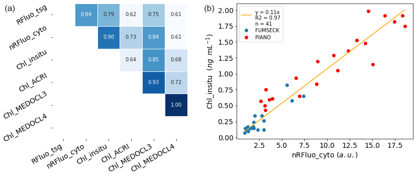
Figure 2Panel (a) shows a correlation plot between different sources of fluorescence and Chl-a concentration estimation per unit volume: fluorescence from the flow-through fluorometer (Rfluo_tsg, a.u., n = 8385); the sum of all phytoplankton cells' normalised red fluorescence from the CytoSense (nRFluo_cyto, , n = 400); and Chl a from in situ discrete sampling (Chl_insitu, ng mL−1, n = 20), from the ACRI ocean colour product for 06:00–18:00 UTC during daytime (Chl_ACRI, ng mL−1, n = 3522), from the MEDOCL3 product for 06:00–18:00 UTC during daytime (Chl_MEDOCL3, ng mL−1, n = 2094), and from the MEDOCL4 product for 06:00–18:00 UTC during daytime (Chl_MEDOCL4, ng mL−1, n = 4498). All of the presented correlations were significant at the 0.01 level using a Pearson test. Panel (b) shows a linear regression between the Chl-a concentration from in situ discrete sampling (Chl_insitu, ng mL−1, n = 41) and the sum of all phytoplankton cells' normalised red fluorescence from the CytoSense (nRFluo_cyto, ). Two data sets are shown using the same instrument (PIANO, “Réaction fonctionnelle, structurelle et journalière des organismes du pico- au nanophytoplancton”, and FUMSECK). The intercept coefficient of the regression was not significant at the 10 % level (t test).
2.5 Fluorescence and chlorophyll a
Different techniques were used during the cruise to estimate Chl-a concentration, and these methods were compared. The absolute Chl-a concentration from Chl_insitu was used as the reference to convert red fluorescence from AFCM and the TSG fluorometer into the Chl-a concentration based on the significant correlations between them (Fig. 2a).
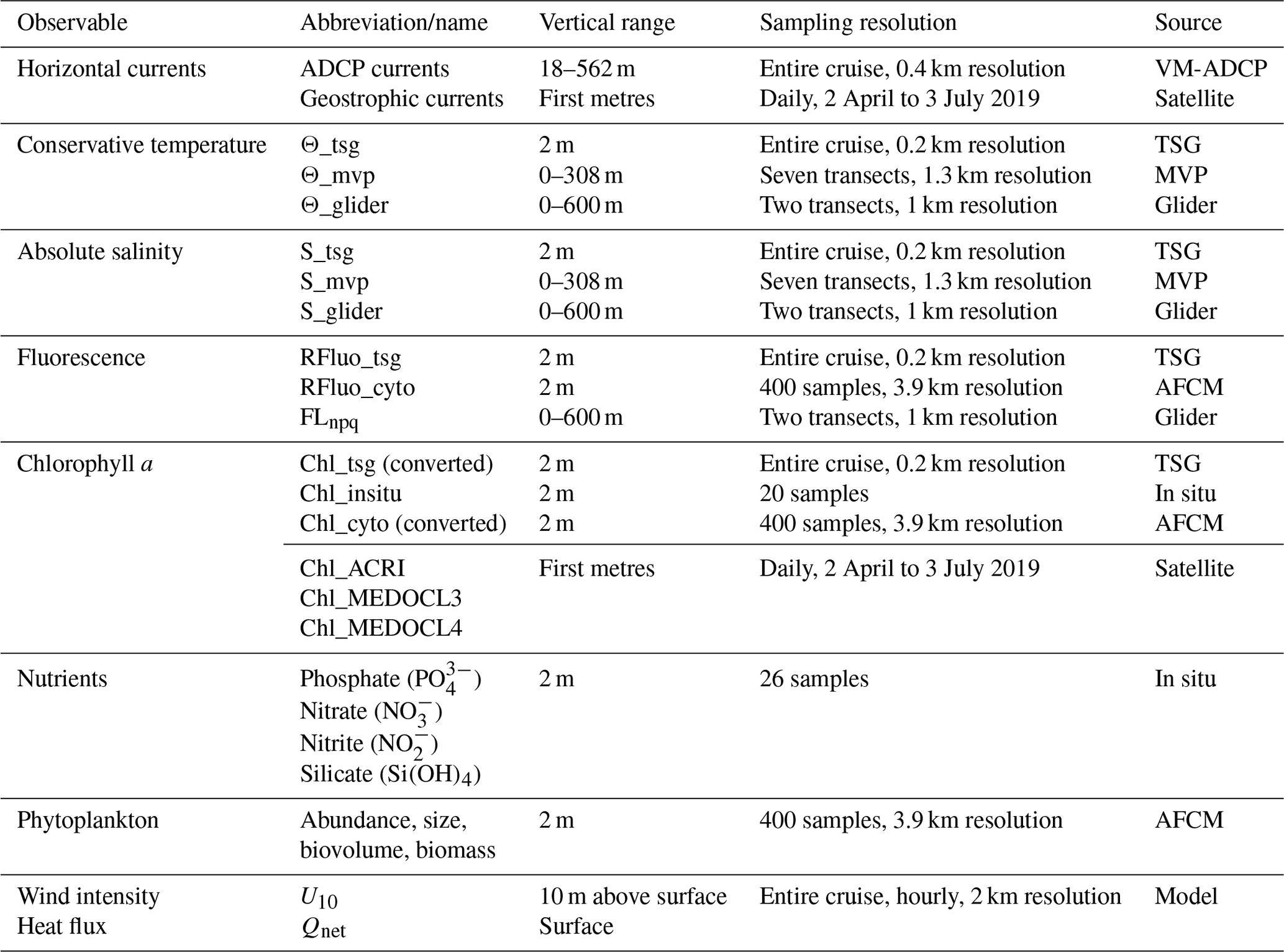
Table 1Summary of the variables measured during the cruise, including their sources, their sampling spatial and temporal resolution, and the vertical range along which they were measured.
Fluorescence from the TSG (RFluo_tsg) was converted into units of Chl-a concentration (Chl_tsg, ng mL−1) using the significant correlation with Chl_insitu as follows: Chl_insitu = 0.85 × Rfluo_tsg − 0.19 (r2 = 0.79, n = 20). The AFCM Chl-a concentration (Chl_cyto) was estimated from the Rfluo_cyto. Values were normalised with 2 µm polystyrene beads (Polysciences, Inc.) and were multiplied by the abundance of each group to get the total normalised Rfluo_cyto per unit volume (nRFluo_cyto, ). nRFluo_cyto was then compared to the Chl_insitu (Fig. 2a, b). A set of samples from a minicosm experiment (PIANO, unpublished data), acquired with the same Chl-a extraction protocol and the same CytoSense instrument, was added to the observations. These samples presented higher Chl-a concentration values, strengthening the relationship. The linear relation between nRfluo_cyto and Chl_insitu was used to estimate the Chl-a concentration for each AFCM phytoplankton group (Chl_cyto, ng mL−1) as follows: Chl_insitu = 0.11 × nRFluo_Cyto (r2 = 0.97, n = 41; Fig. 2b). The origin of the linear regression was not significantly different from zero.
The Chl-a concentration from three different satellite ocean colour algorithms (Chl_ACRI, Chl_MEDOCL3, and Chl_MEDOCL4) were compared to the other sets of Chl-a concentration estimates for sea surface Chl-a validation (Fig. 2a). We performed the association between each Chl_tsg data point and the corresponding Chl satellite data on the same day and for the closest lat/long pixel and then selected those where the Chl_tsg data were between 06:00 and 18:00 UTC (daytime) in order to minimise the effect of night-time extrapolated points. The glider sampling did not follow the ship's route, but a comparison of the 0–5 m signal when the ship–glider distance was smaller than 15 km showed a negligible difference with the ship-adjusted surface Chl-a concentrations (0.04 ± 0.13 ng mL−1).
All of the measurements described above are summarised in Table 1.
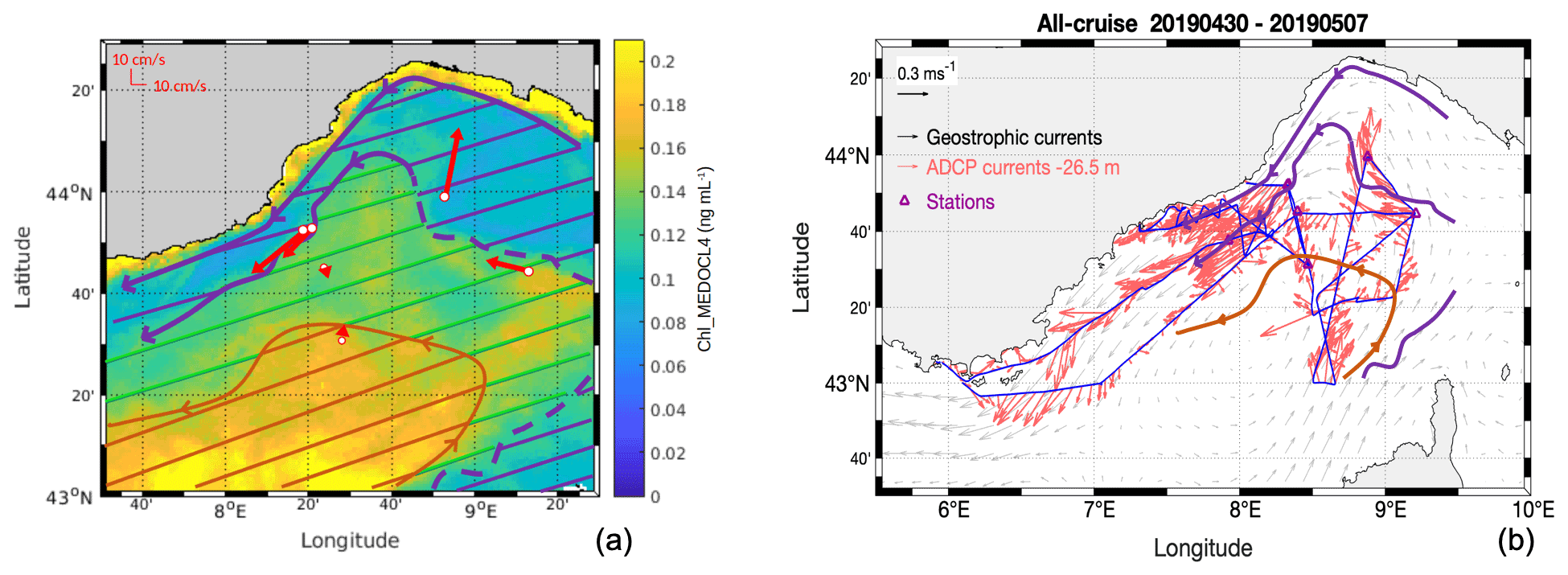
Figure 3Panel (a) presents the satellite Chl-a averaged concentration (Chl_MEDOCL4, ng mL−1) from 1 to 6 May 2019, used to set the drawn hatched boundaries between the hydrodynamic zones, superimposed with horizontal velocities (VM-ADCP, red vectors) at the stations, averaged over 25–150 m. Panel (b) shows the ADCP horizontal currents at 26.5 m depth superimposed on surface geostrophic currents from satellite altimetry.
3.1 Overall circulation
The general oceanic circulation during the FUMSECK cruise is schematised in Fig. 3. In Fig. 3a, the horizontal current velocities averaged over 25–150 m are shown for the seven stations at which the ship stopped, superimposed with the mean Chl-a concentration measured by satellite (Chl_MEDOCL4) from 1 to 6 May 2019. Horizontal current velocities were obtained with the vessel-mounted ADCP, averaged during the 20 min preceding arrival at each station. The boundaries of the different hydrodynamic zones were drawn based on Chl_MEDOCL4 concentration isolines. The region of the NC (purple hatching in Fig. 3a, < 0.12 ng mL−1) corresponds to the lowest Chl_MEDOCL4 concentration. The south-eastern part of the cyclonic recirculation (orange hatching in Fig. 3a, > 0.15 ng mL−1) shows the highest Chl_MEDOCL4 concentrations. These two zones are separated by a region, hereafter referred to as the intermediate zone (green hatching in Fig. 3a, 0.1–0.15 ng mL−1). The vessel-mounted ADCP horizontal currents at 26.5 m depth along the cruise (Fig. 3b) show the high intensity of the NC (0.43 m s−1 mean velocity in the core of the NC) with respect to the cyclonic recirculation zone (0.18 m s−1 mean velocity).
3.2 Storm
During the cruise, an episode of particularly intense winds hit the South of France and the Ligurian Sea. In particular, the Ligurian Sea was exposed to two main winds: north-westerlies (mistral wind) with intensities ranging between 25.8 and 36.1 m s−1 and northerlies (tramontana wind) with intensities ranging between 20.6 and 25.8 m s−1. In this zone, this episode began during the night between 4 and 5 May 2019, reached its maximum intensity on 5 May around 5:00 UTC, and finished on 5 May in the evening. Although the conjunction of these two winds is a classic situation in the Ligurian Sea, this event was particularly intense.
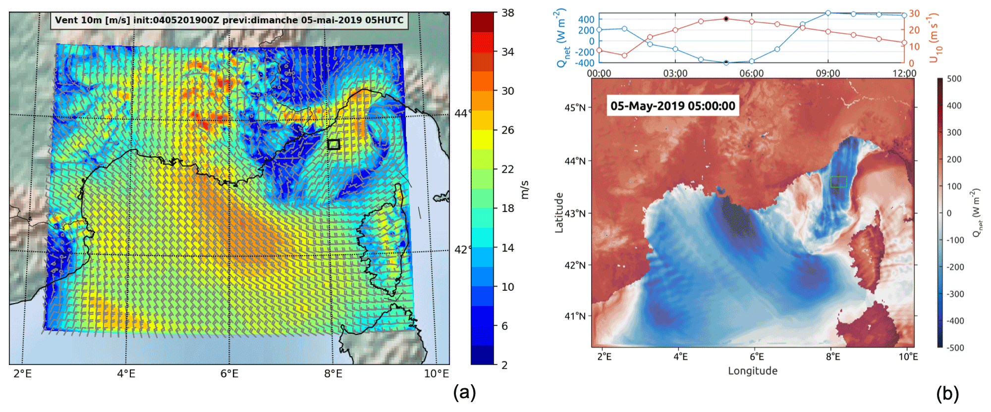
Figure 4Results of the wind situation on 5 May (WRF model WRF-ARW v4.2.1). The black and green squares identify the TSG region of interest sampled 1 d after the storm. Panel (a) presents the wind intensity at 10 m on 5 May at 05:00 UTC. Panel (b) shows the heat flux on 5 May at 05:00 UTC (bottom subpanel) and the temporal distribution of wind intensity and heat flux on 5 May between 00:00 and 12:00 UTC (top subpanel) in the area enclosed by the green square.
After sheltering during the storm, the ship returned to the storm zone during the night between 5 and 6 May. The model shows that, during the storm maximum (5 May at around 5:00 UTC), the ship-sampled zone (marked with squares in Fig. 4) was affected by a wind intensity peak of 26 m s−1 associated with an intense negative net heat flux of −400 W m−2. This sampled zone was in the core of a corridor area (42.5–44.5∘ N, 8∘ E) with strong wind intensities and high negative heat fluxes (Fig. 4).
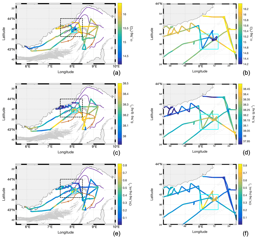
Figure 5Water surface characteristics from TSG along the cruise, superimposed with FSLEs calculated from altimetry showing the (a, b) Θ_tsg , (c, d) S_tsg, and (e, f) Chl_tsg concentration. Panels (a), (c), and (e) show the whole geographic region of the cruise, and panels (b), (d), and (f) illustrate the respective zoom of the indicated region (shown in the black dotted square in the corresponding left panel), identifying the particular TSG region of interest (cyan square) sampled 1 d after the storm.
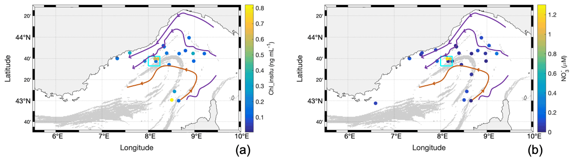
Figure 6Water surface characteristics from discrete in situ sampling along the cruise showing the (a) Chl_insitu concentration and (b) concentration. The cyan square identifies the particular TSG region of interest sampled 1 d after the storm.
3.3 Surface hydrodynamics and hydrology
The general properties of the surface waters include surface conservative temperature, absolute salinity, the Chl-a concentration (Chl_tsg and Chl_insitu), and the in situ nitrate () concentration (Figs. 5, 6). The conservative temperature was globally warmer near the coast and in the NC (mean value of 15.7 ∘C in the NC), whereas it was cooler in the intermediate and recirculation zone (mean value of 15.4 ∘C in the recirculation zone). The absolute salinity was lower near the coast and in the NC (mean value of 38.12 g kg−1 in the NC), whereas it was higher in the intermediate and recirculation zone (mean value of 38.38 g kg−1 in the recirculation zone). The TSG Chl-a (Chl_tsg) concentration mean value was 0.29 ng mL−1 over the whole cruise, with a lower mean value in the NC (0.21 ng mL−1) than in the recirculation zone (0.33 ng mL−1).
When the ship returned to the offshore region less than 24 h after the maximum storm intensity, we observed a patch of low-temperature (< 14.8 ∘C) and high-salinity (> 38.28 g kg−1) water, with a sharp horizontal gradient separating it from surrounding waters (Fig. 5). This patch was associated with an increase in mean Chl a: Chl_insitu rose to 0.65 ng mL−1, whereas the mean value for the whole cruise was 0.25 ng mL−1. Similarly, the maximum Chl_tsg value inside the patch was of 1.11 ng mL−1. The nutrients also showed an increase, in particular the concentration which was up to 1.25 µM, in contrast to a mean value of 0.15 µM for the whole cruise (Fig. 6b). This particular zone of interest is highlighted in cyan in Figs. 5 and 6 and corresponds to longitudes between 8∘ and 8∘15′ E and latitudes between 43∘33′ and 43∘42′ N.

Figure 7Water mass types measured by the MVP (MVP 1 from 30 April at 21:29 to 1 May at 07:50 UTC; MVP 7 from 5 May at 19:22 to 6 May at 05:06 UTC) and the glider (descending southward from 1 May at 08:50 to 4 May at 00:29 UTC; ascending northward from 4 May at 00:29 to 6 May at 03:42 UTC). Panel (a) shows a TS diagram from MVP 7 and ascending glider data. Panel (b) presents a map showing the colour-coded surface waters measured by MVP and the glider as well as the TSG zone of interest. The colours are as follows: recirculation waters are orange, NC waters are yellow, and newly mixed waters are cyan.
A temperature–salinity (TS) diagram was used to describe the water masses (Fig. 7a). The water masses were classified using the absolute salinity S and the conservative temperature Θ, from black for deeper and denser waters (S ≥ 38.61 g kg−1) to lighter orange/yellow tones for the shallower waters (S < 38.61 g kg−1). Hence, surface waters included mostly yellow waters (S ≤ 38.46 g kg−1 for Θ ≤ 13.8 ∘C and S ≤ 38.38 g kg−1 for Θ > 13.8 ∘C) and orange waters (38.38 g kg−1< S ≤ 38.62 g kg−1 and Θ > 13.8 ∘C). As can be seen in Fig. 7b, yellow waters were present at the surface in the NC area and the intermediate zone and will hereafter be referred to as “NC waters”. Conversely, orange waters were localised at the surface offshore in the recirculation zone of the basin-scale cyclonic circulation and will hereafter be called “recirculation waters”.

Figure 8Vertical transects versus longitude with associated coloured waters from (a) MVP 1, (b) MVP 7, (c) descending glider data (southward transect), and (d) ascending glider data (northward transect).
A cold-surface-water patch was encountered by the ship after the storm in the geographical cyan area shown in Fig. 5 as well as during the storm by the glider in its ascending route (Fig. 11a). The characteristics of this cold-surface-water patch (38.31 g kg−1 ≤ S ≤ 38.45 g kg−1 for 14 ∘C ≤ Θ ≤ 14.5 ∘C and 38.28 g kg−1 ≤ S ≤ 38.38 g kg−1 for 14.5 ∘C ≤ Θ ≤ 14.78 ∘C) are superimposed in cyan on the TS diagram. They correspond to either NC or recirculation waters, with a density anomaly around 28.37–28.70 kg m−3, and are present around 30–40 m depth before the storm, as can be seen in Fig. 8a. Between 43∘31′ and 43∘39′ N, these waters have been detected between 50 m and the surface, by both the MVP during transect 7 (after the storm) and the glider at the end of its ascending route during the storm (Fig. 8b). These waters, hereafter called “newly mixed waters”, were present up to the surface in a very localised spot in space and time (Fig. 7c), and they are represented in cyan through the paper. The vessel crossed these surface newly mixed waters on 6 May between 02:32 and 02:53, 03:03 and 04:03, and 05:32 and 11:36 UTC, with the vessel moving in and out of these waters. The glider encountered the surface newly mixed waters on its way north at around 10:00 UTC on 5 May. It was about 85 km from the ship at this time and stayed in these waters until its recovery on the morning of 6 May.
3.4 Chlorophyll a and total biomass
Chl_insitu varied between 0.07 and 0.82 ng mL−1 with a mean ± SD of 0.25 ± 0.21 ng mL−1, with 20 samples collected all along the cruise (Figs. 6a, 9a). The standard deviations are representative of the spatiotemporal variability, not the measurement errors. Chl_cyto values followed a similar trend with minimal and maximal values of 0.03 and 0.94 respectively and a mean ± SD of 0.26 ± 0.16 ng mL−1 (Fig. 9a). Chl_tsg varied between undetectable values and 1.11 ng mL−1, with a mean of 0.29 ± 0.16 ng mL−1 and a mean spatial resolution of 0.16 km with a total of 8385 points (Figs. 5e, 9b).
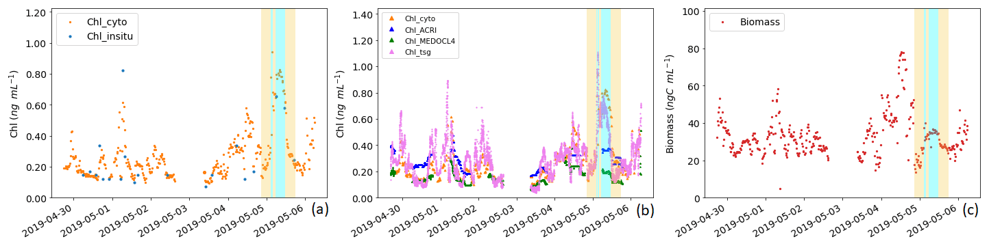
Figure 9Panel (a) presents a comparison between the surface Chl-a concentration measured in situ (Chl_insitu, ng mL−1) and the Chl-a concentration estimation obtained from AFCM (Chl_cyto, ng mL−1). Panel (b) presents a comparison between the surface Chl-a concentration estimated by AFCM (Chl_cyto), ACRI (Chl_ACRI), MEDOCL4 (Chl_MEDOCL4), and the fluorometer (Chl_tsg). Panel (c) shows the total surface phytoplankton biomass variation throughout the cruise (ng C mL−1). The periods corresponding to the surface crossing of the newly mixed waters (in cyan) and the surrounding NC waters (6 h before and after the newly mixed ones, in yellow) are indicated.
Ocean colour Chl-a match-ups with Chl_cyto (Fig. 9b) were significantly higher for Chl_ACRI than for Chl_MEDOCL4 (0.27 ± 0.07 and 0.15 ± 0.05 ng mL−1 respectively; p < 0.001, block bootstrap test; Appendix D). Maximal values of Chl_ACRI and Chl_MEDOCL4 (0.48 and 0.51 ng mL−1 respectively) were below the maximal values of Chl_cyto and Chl_tsg.
Total biomass of phytoplankton ranged between 13.75 and 77.94 ng C mL−1 with a mean ± SD of 33.05 ± 11.23 ng C mL−1 and followed Chl_cyto trends, with a correlation of 0.52 (n = 400) when considering the entire data set and a correlation of 0.72 (n = 382) when removing data from the newly mixed waters. For the newly mixed waters, the correlation was 0.78 (n = 21).
Table 2The mean and standard deviation of surface abundance, size (equivalent spherical diameter, ESD), biovolume per cell, biomass per cell, Chl a per unit volume (Chl_cyto), biomass per unit volume, and the biomass / Chl_cyto ratio for the all waters sampled (“Overall”, n = 400), the NC surrounding waters (n = 20), and the newly mixed waters (n = 43) (see Fig. 7) for the five AFCM phytoplankton groups identified. The surrounding NC waters correspond to the surface NC waters acquired 6 h before and after the ship entered newly mixed waters. A moving block bootstrap test between NC surrounding and newly mixed waters reveals significant differences, and bold values are significantly different at a Bonferroni-corrected 5 % level.
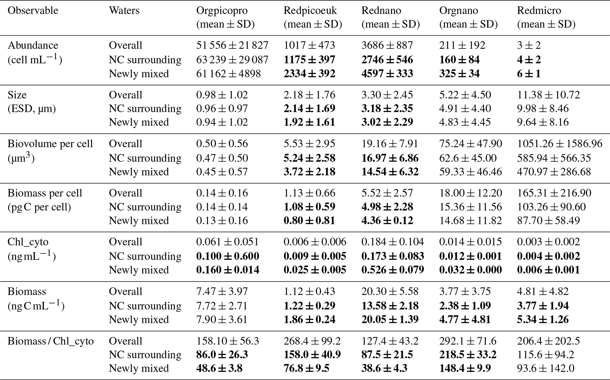
3.5 Phytoplankton groups and reaction
The most abundant group was the Orgpicopro, followed by the Rednano, Redpicoeuk, Orgnano, and Redmicro (see Table 2). Inversely, the Rednano biomass was the highest, followed by the Orgpicopro biomass. Redpicoeuk biomass was the lowest. Chlorophyll per group per unit volume regarding the overall study area was also the highest for the Rednano followed by the Orgpicopro. The biomassChl_cyto ratio was above 127 for all phytoplankton groups when considering the entire study area.

Figure 10Illustration of the newly mixed waters (corresponding to the cyan background) and their direct surroundings (NC waters, corresponding to the yellow background), in terms of surface temperature, salinity, and biomass per phytoplankton group (ng C mL−1). Panel (a) presents variation in the surface absolute salinity (blue dots) and surface conservative temperature (orange dots). Panel (b) shows variation in the surface biomass for the Redpicoeuk (orange line), Orgpicopro (red line), and Orgnano (green line) groups. Panel (c) presents variation in the surface biomass for the Rednano (violet line) and Redmicro (black line) groups. The vertical axis label colours indicate the associated curve. Similarly, labels and titles written in two different colours indicate that two curves are associated with the same axis.
For all phytoplankton groups except for Orgpicopro, abundances and biomass per unit volume were twice as high in newly mixed waters (cyan in Fig. 7a) compared with NC surrounding waters (yellow in Fig. 7a), as shown in Table 2 and Fig. 10. All groups had higher Chl-a values in the newly mixed waters (Table 2). Conversely, the Rednano and Redpicoeuk estimated average sizes were higher with a concomitant higher biomass per cell in the NC surrounding waters than in the newly mixed waters (Table 2). The biomass / Chl_cyto ratios were lower in NC waters and lower still in newly mixed waters compared with the overall area (see Fig. 13) for all groups, despite a lower carbon content per cell. In short, the newly mixed waters evidenced higher abundances and a higher Chl-a concentration and biomass per unit volume but smaller sizes and biomass per cell (mainly for Redpicoeuk and Rednano).

Figure 11Glider profiles of (a) conservative temperature and (b) absolute salinity. The coloured squares correspond to the dominant water mass (according to Fig. 7) observed at 10 m depth by the glider. The dashed vertical line represents the time separating the descending and ascending transects.
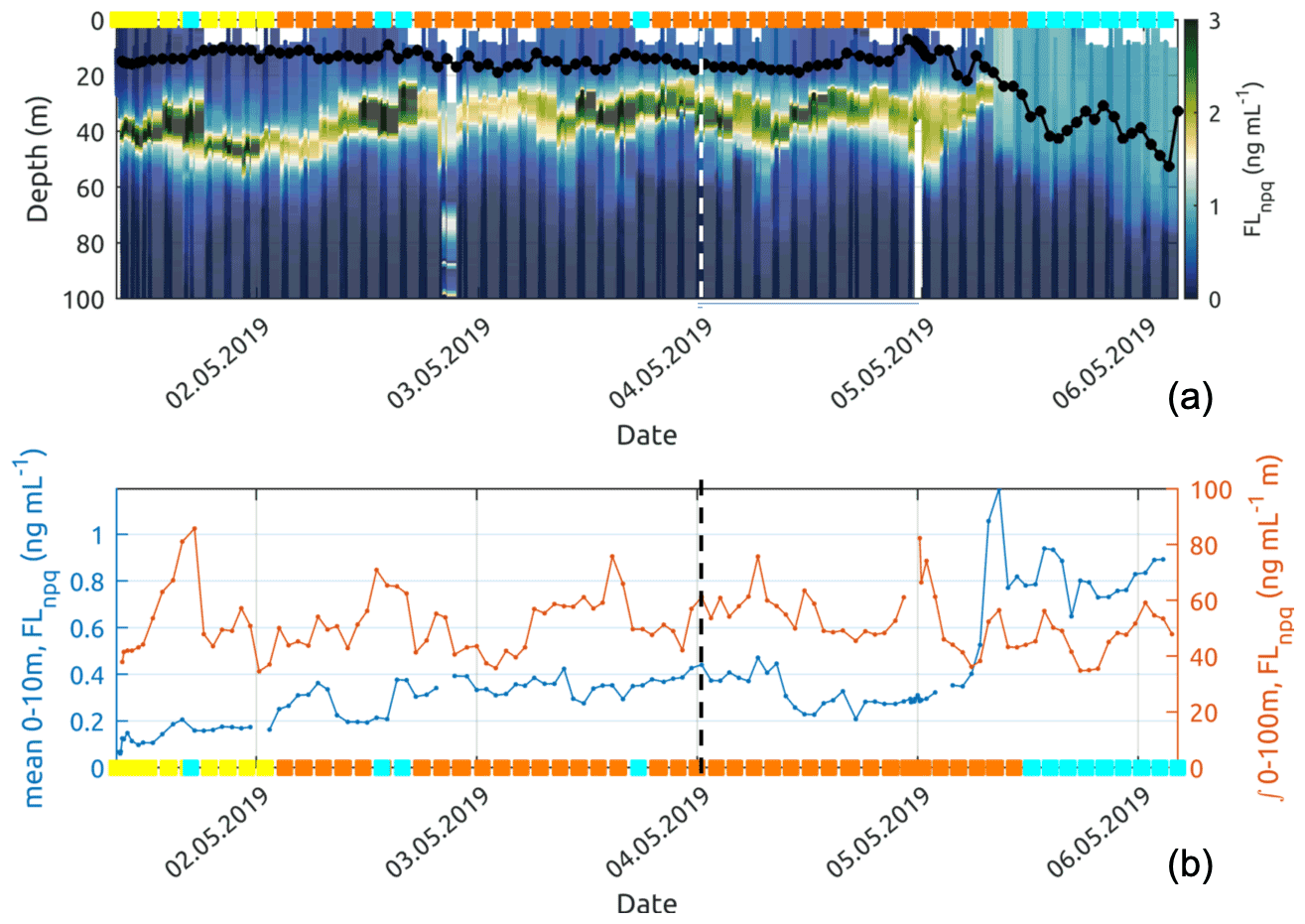
Figure 12Panel (a) shows the fluorescence observed by the glider and corrected using non-photochemical quenching following Xing et al. (2012). The black line with dots shows the mixed-layer depth (MLD) for each glider profile. Panel (b) presents the near-surface (0–10 m average) Chl-a fluorescence concentration and the Chl-a fluorescence concentration integrated over 0–100 m along the glider track. The coloured squares correspond to the dominant water mass (according to Fig. 7) observed at 10 m depth by the glider. On both plots, the dashed vertical lines represent the time separating the descending and ascending transects.
3.6 Subsurface fluorescence signal observed by the glider
Referring to the surface water masses of Sect. 3.3, the glider entered the newly mixed surface waters on its northward return transect (5 May), leaving behind recirculation waters (Fig. 7c). Down to approximately 60 m depth, the surface temperature and salinity steeply decreased (see Fig. 11), moving from recirculation waters to newly mixed waters. The fluorescence near the surface increased rapidly by a factor of 4 (Fig. 12b) as the mixed-layer depth recorded by the glider deepened from 15 to 50 m (Fig. 12a). However, the integrated fluorescence content in the upper 100 m did not show any noticeable variation (Fig. 12b).
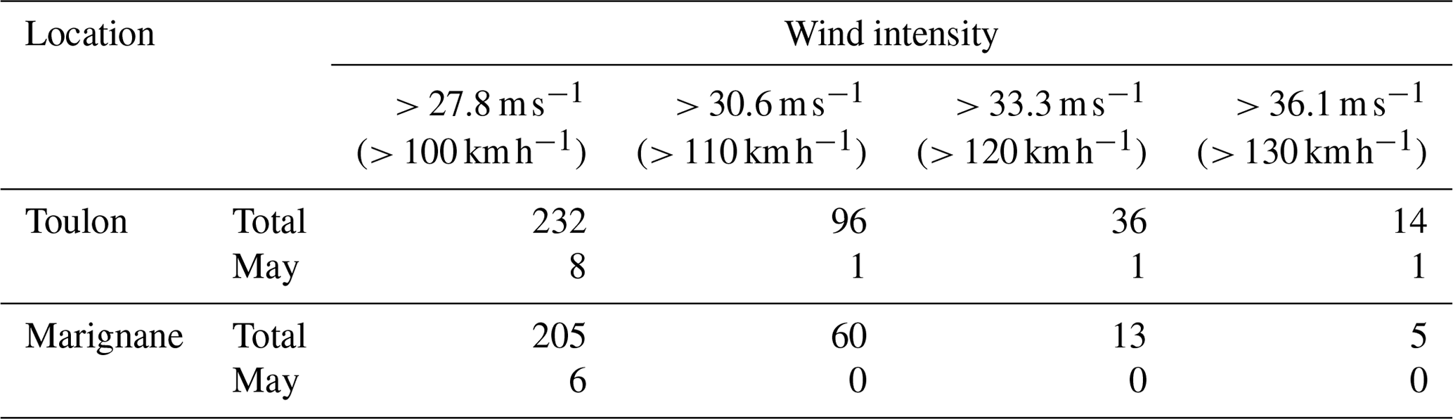
In the NW Mediterranean Sea, the water column is generally well stratified in May with nearly undetectable surface nutrient availability (Pasqueron De Fommervault et al., 2015). This was indeed the oceanographic setting before an intense storm dominated by north-westerly winds impacted the water column. The analysis of 30 years of coastal data in the South of France (Toulon and Marignane) by Meteo France shows that the typical periods of intense wind occur at the end of winter and middle of autumn. In Toulon, winds with an intensity > 27.8 m s−1 occur on average 8 times per year, although only once every 4 years in May; winds with an intensity > 36.1 m s−1 occur on average once every 2 years and once every 30 years in May. The total occurrence of different wind intensities for the whole 1981–2010 period is shown in Table 3. The wind intensity of the studied storm, which reached a maximum of 36.1 m s−1, was rare in the Mediterranean Sea, and it was similar to the average wind intensity of the typhoons studied by Wang (2020).
Table 3The occurrence of different wind intensity events during the 1981–2010 period in the South of France for the entire (Total) period and for May only (http://tempetes.meteo.fr/spip.php?article221, last access: 5 January 2023).
The physical and biogeochemical data, collected thanks to the deployment of high-resolution sensors, showed a clear shift in the local ocean physical–biological conditions after the storm. These changes included a steep change in temperature and salinity as well as increases in surface Chl-a concentrations and surface phytoplankton biomass and abundances.
Overall, the abundances of Redpicoeuk and Rednano were more than twice as high in April during the MERITE-HIPOCAMPE cruise (Boudriga et al., 2022) than during the FUMSECK cruise, suggesting that the FUMSECK cruise occurred after the spring bloom events when nutrients in the euphotic layer are consumed. Only Orgpicopro, which is related to Synechococcus cells, was similar during both sampling efforts. Abundances of Orgnano, Redpicoeuk, and Rednano were close to those in the eastern Mediterranean Sea in May (Latasa et al., 2022). Conversely, the abundances of phytoplankton groups during FUMSECK were twice as high on average as those observed at the same location during the OSCAHR (Observing Submesoscale Coupling At High Resolution) cruise in November 2015 (Marrec et al., 2018) for the Rednano and Orgpicopro groups but similar for the Redpicoeuk group. The size of Rednano was smaller on average (−20 %) than that observed during the OSCAHR cruise, but the size of the Redpicoeuk (+30 %) and the Orgpicopro (+20 %) was larger.
The conversion of the total red fluorescence to Chl a showed that Rednano is the main contributor during the entire study. The same observation held in terms of biomass. All groups exhibited higher Chl_cyto in the newly mixed waters with respect to the surrounding waters, reaching up to +68 % for Rednano in the newly mixed waters compared with the NC surroundings, despite the cells being smaller. Similarly, fluorescence per group was much higher in the cold core of the OSCAHR eddy than in the surrounding warm water. During OSCAHR, the Chl-a ratio reached 1.5 between the cold and the warm waters, whereas Chl_cyto for Rednano and Redpicoeuk was nearly 3 times higher in the cold newly mixed waters in our study. This suggests that the cells did not have time to photoacclimate or that different species were involved. Indeed, the newly mixed water was sampled less than 1 d after deeper layers reached surface layers.
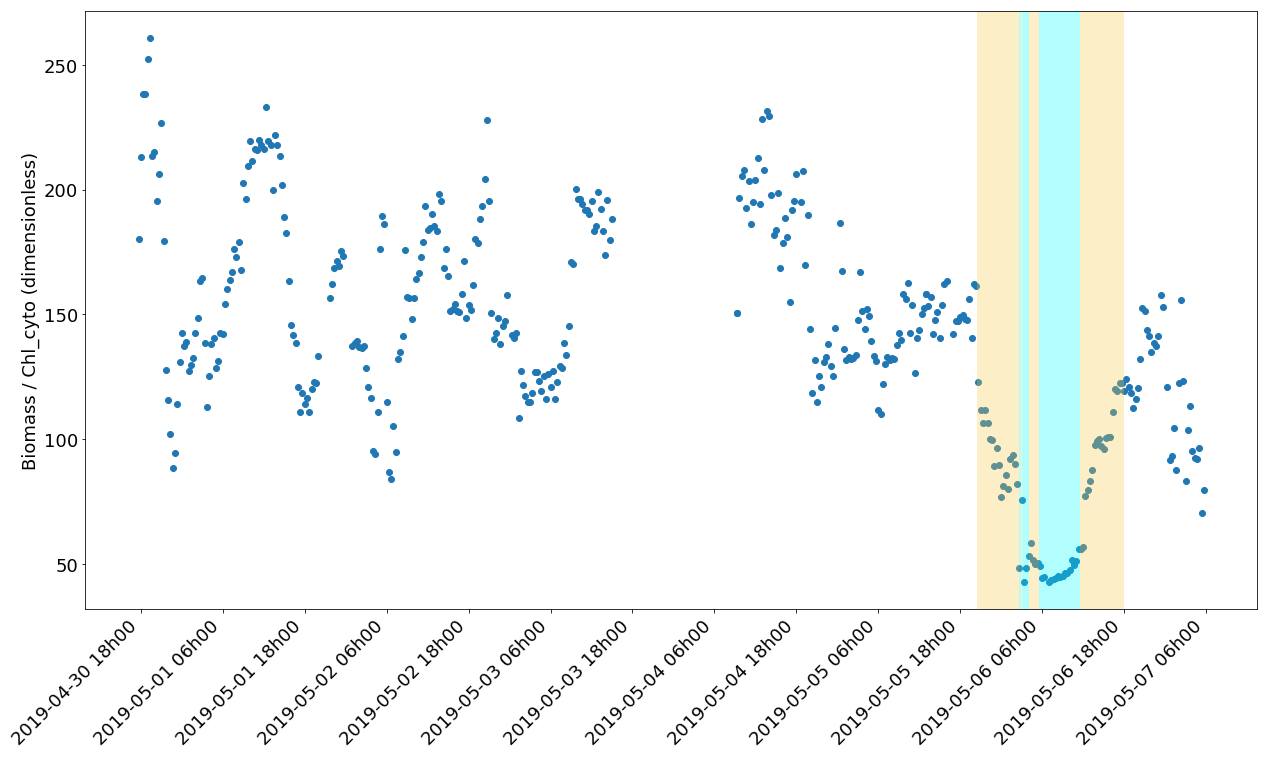
Figure 13Evolution of the biomass (ng C mL−1) Chl_cyto (ng mL−1) ratio through the cruise. The yellow and cyan colour spans correspond to the water masses in Fig. 10.
The phytoplankton abundances and size class distributions provide information on the capacity of the area to sustain the marine food web, while the carbonChl-a ratio is an indicator of the photoacclimation status and is especially interesting when primary production is calculated from Chl a only (Behrenfeld et al., 2002). It also provides insight into the rapid changes in light conditions, as some time is needed to photoacclimate, and adjust the pigment content of a cell to the new light conditions (Lewis et al., 1984). Most of the carbonChl-a estimates are bulk, and only a few studies have attempted to convert values per size class. This paper aims to contribute to the estimated ratio from field studies with much higher precision thanks to the clear separation between phytoplankton and bulk particulate organic carbon given by AFCM and due to the resolution at the single-cell level. The estimation of the cell carbon biomasses could be biased by the errors made during the prior estimation of the cell biovolumes as well as by the use of biovolume-to-biomass conversion factors from the literature. Nevertheless, the high variability in the carbon/Chl-a values between phytoplankton groups evidenced different metabolisms between groups, with Redpicoeuk having a much higher ratio (268.4) than Rednano (127.4). The Redpicoeuk carbon / Chl-a ratio range outside the newly mixed waters was similar to the highest values found in summer in the study of Calvo-Díaz et al. (2008), where values for picoplankton varied seasonally from 0.07 to 282. Inside the newly mixed waters, Redpicoeuk carbon / Chl-a values were similar to those in the northern European seas in summer, in higher-nutrient environments with lower-light conditions (maximal values were close to 85 in open waters; Jakobsen and Markager, 2016). The carbonChl-a ratio integrating all groups varied from approximately 90 to 250 under surface conditions but dropped down to 50 in the newly mixed waters (Fig. 13). The high ratios observed before the storm could reflect the high-light and low-nutrient conditions of the post-bloom oligotrophic period sampled in the Ligurian Sea. The remarkable drop in the ratio observed in the cold-water patch could be a signature of a sudden change in phytoplankton cells that may have translated the not yet photoacclimated configuration of the cells to high-light conditions (Jakobsen and Markager, 2016).
While surface observations alone suggested a rise in Chl-a concentrations (Figs. 5, 6), the integrated Chl-a values from the glider fluorometer rather suggested that this surface increase is due to a dilution of the deep chlorophyll maximum in the mixed layer during the storm (Fig. 12). The deepening of the mixed-layer depth can lead to the dilution – by vertical mixing – of phytoplankton cells previously concentrated in the deep chlorophyll maximum.
Typhoons can be compared to the type of storm observed in our study with respect to the intensity and duration of the winds triggering a fast decrease in surface temperature and an increase in surface Chl a. Most typhoons enhance the chlorophyll surface concentration (Wang, 2020). In open-water tropical and subtropical areas, the dilution phenomenon of the deep chlorophyll maximum after typhoons has been said to be a source of overestimation of potential phytoplankton production when using only satellite observation, as the nitracline is not always affected (Chai et al., 2021) and Chl a from the deep chlorophyll maximum is not always related to higher biomass and production (Marañón et al., 2021). The increase in Chl a after the deepening of the mixed-layer depth in post-bloom periods caused by wind events is not obvious, as demonstrated by Andersen and Prieur (2000). In our case, the deepening of the mixing due to the storm was accompanied by an increase in surface nutrients that could only be linked to the uplift of the nitracline, as we were far enough from coastal run-off influences. This mixing was related to the spreading and increase of the phytoplankton in the upper layer in terms of biomass and Chl a. In addition, mixing could lead to a possible dilution of grazers, favouring pico- and nanophytoplankton accumulation in the shallowing mixed layers a few days after (Morison et al., 2019). This could, in turn, foster integrated primary production by enhancing the phytoplankton division rate and biomass (Behrenfeld, 2010) which, when grazers are diluted, is related to higher organic carbon export efficiency (Henson et al., 2019). This phenomenon has also been observed after winter storms in the Sargasso Sea, where diatoms' increase was maximal within 2 d after shoaling of the mixed-layer depth (Krause et al., 2009). These pulse production events could be responsible for up to 20 % of the global primary production in the Sargasso Sea (Lomas et al., 2009).
Our observations captured the short-term physical and phytoplankton response to a storm. Although rapid and strong changes were observed, we did not have the possibility to follow in situ post-storm conditions. Although they are not representative of what happens in the entire mixed water column, satellite data showed an effect on surface temperature and Chl a within the ship–glider storm geographical zone (latitudes between 43∘30′ and 43∘42′ N and longitudes between 8∘ and 8∘30′ E). In this zone, the mean SST was lower during the 4 d following the storm (6–10 May, 14.8 ∘C) than in the 20 April–20 May period (15.1 ∘C), whereas the mean Chl_ACRI value was higher (0.44 ng mL−1 compared with 0.32 ng mL−1), suggesting that the pico- and nanophytoplankton size classes could have had time to grow and accumulate, as their growth rate is close to one to two divisions per day when nutrients and light are available (Morison et al., 2019). This is supported by the increase in the particulate organic carbon concentration (POC, https://oceancolor.gsfc.nasa.gov/atbd/poc/#sec_6, last access: 5 January 2023, MODIS Aqua L3 product) in the considered zone. Indeed, a higher POC concentration is observed during the 4 d following the storm (6–10 May, 104.1 ng mL−1) compared with the 20 April–20 May period (88.7 ng mL−1), suggesting that the whole trophic chain may be impacted by the storm.
During the FUMSECK cruise, the deployment of high-spatiotemporal-resolution instruments made it possible to observe the link between fine-scale physical structures and the phytoplankton size class distribution in the Ligurian Sea. Initially, the studied area showed typical post-bloom physical and biological characteristics of the NW Mediterranean Sea with surface stratified conditions, a mixed-layer depth of about 15 m, and almost undetectable surface concentrations of chlorophyll, where cells < 4–5 µm dominated biomass. A high-intensity storm occurred during the cruise period, and its effects on the water column and the surface phytoplankton were specifically studied thanks to high-resolution measurements, performed simultaneously using a glider, an MVP, a surface thermosalinometer, a VM-ADCP, and an automated flow cytometer. The in situ data set was strengthened by satellite and numerical modelling data.
The area affected by the storm was characterised by waters mixed from depths down to 60 m up to the surface, with a clear dilution of the deep chlorophyll maximum, leading to abrupt changes in the phytoplankton abundances in surface waters. The study of phytoplankton at the single-cell level showed clear physiological changes with a drop in the carbonChl-a ratio associated with an increase in abundances and biomass. These physiological shifts can be regarded as a reaction to the sudden changes. The storm, although identified as a rare event in this area, should be considered an important feature to study with respect to fine-scale physical–biological coupling, especially under stratified surface oligotrophic conditions where nutrient increases can trigger pulse production and affect global biogeochemical budgets.
These results pave the way for future oceanic cruises, and in particular for the BioSWOT-Med cruise in 2023. This cruise is planned as part of the “Adopt a Cross Over” initiative that organises simultaneous oceanographic cruises around the world during the fast-sampling phase of the new satellite SWOT (Surface Water and Ocean Topography) (d'Ovidio et al., 2019), which will allow the precise observation of fine-scale ocean dynamics. The aim is to study the fine-scale features and their influence on biology, with methodology supporting offshore, multi-instrumental, multi-technique, multi-scale, and multi-disciplinary observations.
These results highlight the need for concomitant observations of physics and biology with high spatiotemporal resolution in order to understand the effect of physical forcing events, such as storms, on marine ecosystems. Considering that changes in both the frequency and the intensity of Mediterranean storms are expected (Lionello et al., 2006; Flaounas et al., 2021), these results may help to estimate the impact of climate change on the ecology and biogeochemistry of the Mediterranean Sea.
The phytoplankton groups were identified on dimensionless cytograms by comparing (two by two) the optical pulse shapes per cell, as collected by the CytoSense flow cytometer (Fig. A1). The groups were manually gated. The names of the groups were decided prior to the publication of Thyssen et al. (2022) and will be coupled to their standard names in the open-access data set.
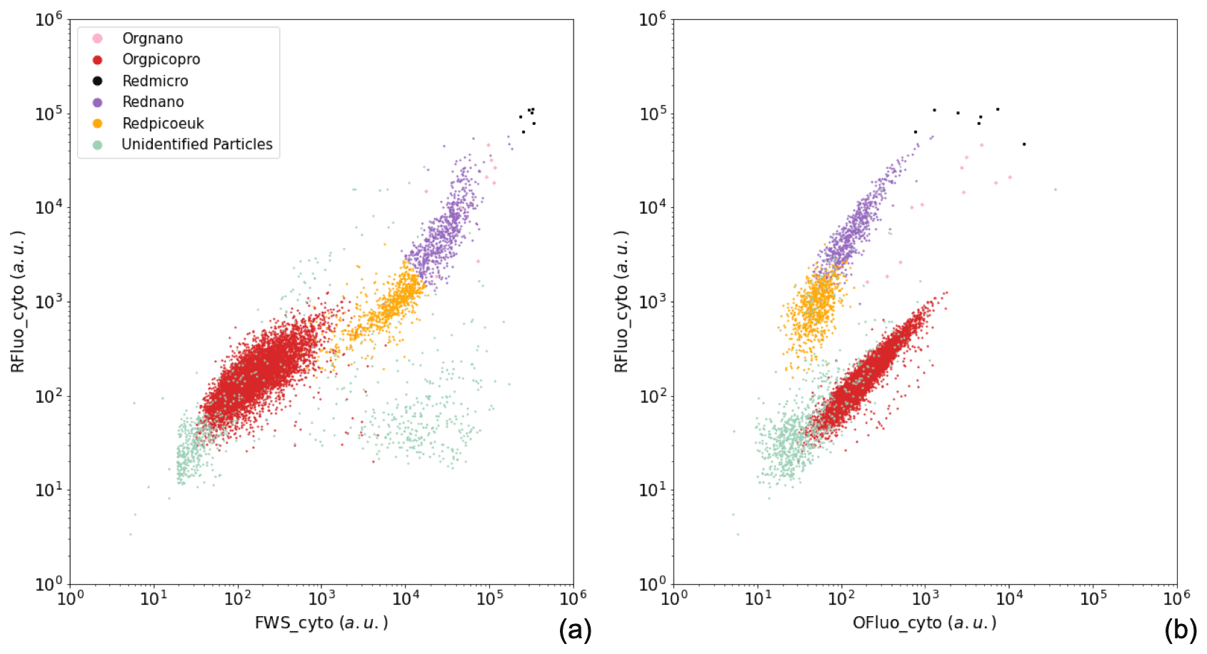
Figure A1Manual identification of the main phytoplankton functional groups. Two-dimensional cytograms representing the following are shown: (a) the area under the curve of red fluorescence (RFluo_cyto, a.u.) versus forward scatter (FWS_cyto, a.u.) of each particle, depicting the main cytometric functional groups identified, namely Orgnano (pink dots), Orgpicopro (red dots), Redmicro (black dots), Rednano (purple dots), Redpicoeuk (orange dots), and the Unidentified particles group (green dots); (b) the area under the curve of red fluorescence (RFluo_cyto, a.u.) versus orange fluorescence (Ofluo_cyto, a.u.) of each particle, evidencing the same groups. The size of the Orgnano and Redmicro points located in the top right-hand part of the cytograms was increased in order for them to be visible, as these groups comprise very few cells in each sample.
No pre-cruise calibration of the ECO Puck glider was carried out. Nevertheless, we observe good statistical agreement between the glider measurements and those taken from the ship TSG (Fig. B1). Over a sample of N = 33 glider profiles where the glider–ship distance is lower than 40 km, surface Chl a from the ship TSG (Chl_tsg) and the Chl a 0–10 m average from the glider have a correlation coefficient of R = 0.76 (with a significant p value of 2.5 × 10⁻⁷) and a mean standard error of 0.067 ng mL−1, which is well below of the amplitude of the observed signal during the storm (maximum Chl_tsg of 1.11 ng mL−1). Values from the onset of the storm have been excluded (grey values after 5 May) because the glider was experiencing different conditions compared with the ship, which was sheltering from the bad weather. At the end of the time series, when the glider was recovered, the values between the two platforms again agree well, which provides good confidence in the Chl-a fluorescence signals described by the glider's sensor during its mission.
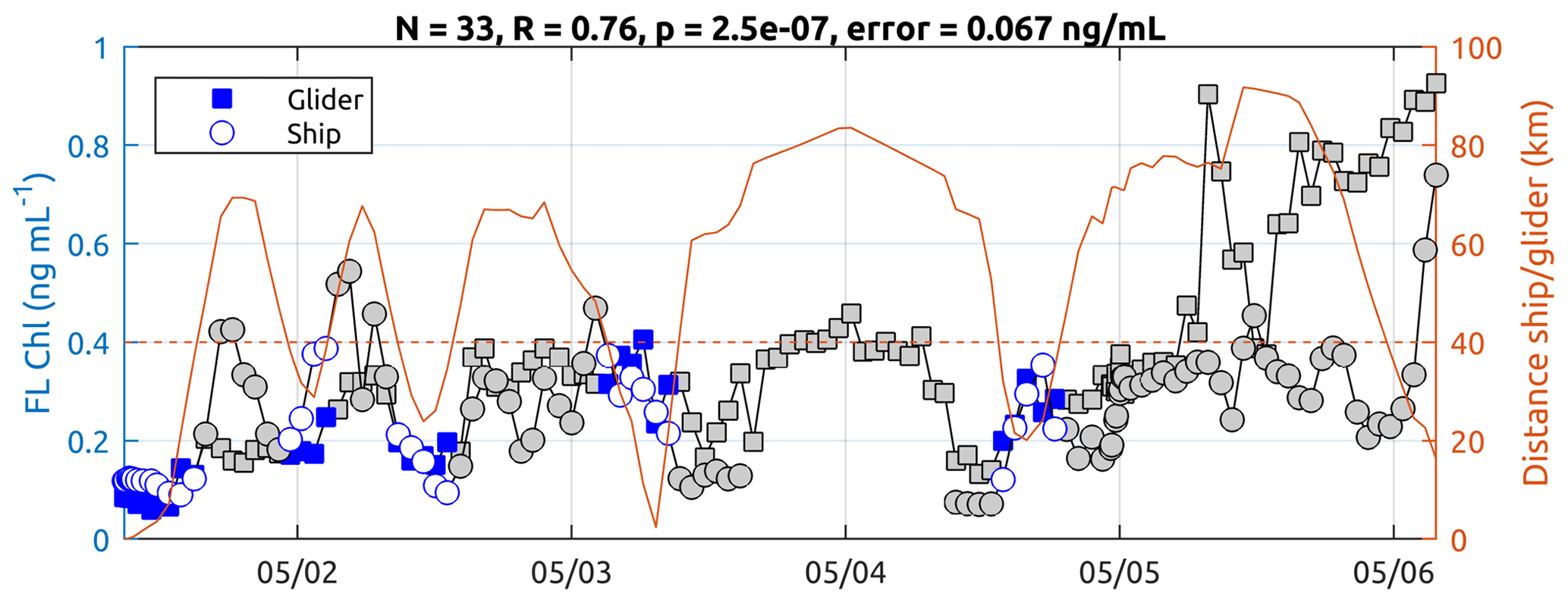
Figure B1Comparison of Chl a between the ship TSG and the 0–10 m average from the glider. The numbers indicated on top of the figure and the blue markers correspond to measurements where the glider–ship distance is lower than 40 km.
The satellite products exploited for FUMSECK are outlined in this section (Barrillon et al., 2020).
For the SSH and associated geostrophic currents, we utilised the “Mediterranean ocean gridded L4 Sea Surface Heights and derived variables” data set (SEALEVEL_MED_PHY_L4_NRT_OBSERVATIONS_008_050, now SEALEVEL_EUR_PHY_L4_NRT_OBSERVATIONS_008_060, https://resources.marine.copernicus.eu/product-detail/SEALEVEL_EUR_PHY_L4_NRT_OBSERVATIONS_008_060/INFORMATION, last access: 5 January 2023), which is a 0.125∘ × 0.125∘, multi-satellite product.
For SST, we employed two data sets. The first product is the “Mediterranean Sea – High Resolution and Ultra High Resolution L3S Sea Surface Temperature” data set (SST_MED_SST_L3S_NRT_OBSERVATIONS_010_012, https://resources.marine.copernicus.eu/product-detail/SST_MED_SST_L3S_NRT_OBSERVATIONS_010_012/INFORMATION, last access: 5 January 2023), which is a 0.01∘ × 0.01∘ product with a strict temporal window (local night-time) to avoid diurnal cycle and cloud contamination that provides super-collated (merged multi-sensor, L3S) SST data remapped over the Mediterranean Sea.
The second product is the “Mediterranean Sea High Resolution and Ultra High Resolution Sea Surface Temperature Analysis” (SST_MED_SST_L4_NRT_OBSERVATIONS_010_004, https://resources.marine.copernicus.eu/product-detail/SST_MED_SST_L4_NRT_OBSERVATIONS_010_004/INFORMATION, last access: 5 January 2023), which is a 0.01∘ × 0.01∘, night-time image, multi-satellite product.
For Chl a, we employed three data sets. The first product is the “Global ocean Chlorophyll from satellite observations” data set (OCEANCOLOUR_GLO_CHL_L3_NRT_OBSERVATIONS_009_032, now OCEANCOLOUR_GLO_BGC_L3_NRT_009_101, https://resources.marine.copernicus.eu/product-detail/OCEANCOLOUR_GLO_BGC_L3_NRT_009_101/INFORMATION, last access: 5 January 2023), which is a 4 km × 4 km, ACRI-ST company, multi-satellite product, hereafter called Chl_ACRI. The second product is the “Mediterranean Sea surface Chlorophyll concentration from multi satellite observations” data set (OCEANCOLOUR_MED_CHL_L3_NRT_OBSERVATIONS_009_040, now OCEANCOLOUR_MED_BGC_L3_NRT_009_141, https://resources.marine.copernicus.eu/product-detail/OCEANCOLOUR_MED_BGC_L3_NRT_009_141/INFORMATION, last access: 5 January 2023), which is a 1 km × 1 km, multi-satellite product, hereafter called Chl_MEDOCL3. Finally, the third product is the “Mediterranean Sea daily interpolated surface Chlorophyll concentration from multi satellite observations” data set (OCEANCOLOUR_MED_CHL_L4_NRT_OBSERVATIONS_009_041, now OCEANCOLOUR_MED_BGC_L4_NRT_009_142, https://resources.marine.copernicus.eu/product-detail/OCEANCOLOUR_MED_BGC_L4_NRT_009_142/INFORMATION, last access: 5 January 2023), which is a 1 km × 1 km, multi-satellite product, hereafter called Chl_MEDOCL4.
The significance of the differences in the means of each phytoplankton group between water types was tested using two-tailed tests based on the moving block bootstrap principle (Liu and Singh, 1992). Using a bootstrap-based test avoided assuming that the observations were mutually independent and have to follow Gaussian distributions (given the small sample size in each water type). These assumptions were indeed violated in our case. Instead, the stationarity of the samples originating from each water mass was assumed. Sampling the observations by blocks of adjacent observations preserves the serial autocorrelation existing in the sample. The size of the blocks is, in practice, left to the practitioner. and values in the [1, 4] range were tested and did not influence the results. The number of bootstrap samples used to perform the tests was 3000 draws. The level of the tests was 5 % with a Bonferroni correction (Dunn, 1961) to account for multiple-hypothesis testing.
The data used in this work are available from https://doi.org/10.17600/18001155 (Barrillon, 2019).
JLF prepared the instruments prior to the cruise, and JLF SB, AMD, GG, MT, and RT deployed them on board. AAP operated SPASSO and analysed the water masses, and CC analysed the current data. GG and MT prepared and operated the flow cytometer, and MT and RF analysed and interpreted the flow cytometry data. NB prepared and piloted the glider, FC performed the first treatment of the glider data, and AB analysed the glider data. CY performed the model data, and CY and AB analysed the model data. AMD analysed the MVP data. Fd'O and AMD initiated the project. SB designed the experiment, led the research, and prepared the manuscript with contributions from all co-authors. All authors contributed to the manuscript.
The contact author has declared that none of the authors has any competing interests.
Publisher's note: Copernicus Publications remains neutral with regard to jurisdictional claims in published maps and institutional affiliations.
We thank the captain and the crew of the RV Téthys II for the cruise and their help with the deployment of the instruments. This research was supported by CNES (BioSWOT project) and by the French National programme LEFE (Les Enveloppes Fluides et l'Environnement) FUMSECK-vv project (PIs Stéphanie Barrillon and Anne A. Petrenko). The flow cytometer was funded by the CHROME (PI Melilotus Thyssen, financially supported by the Excellence Initiative of Aix-Marseille University – A*MIDEX, a French “Investissements d'Avenir” program), and FEDER funding (PRECYM flow cytometry platform). The authors thank Nicole Garcia and Patrick Raimbault from the MIO-PACEM platform for the chlorophyll-a and nutrient analyses. SPASSO is operated with the support of the SIP (Service Informatique de Pythéas), in particular Christophe Yohia, Julien Lecubin, Didier Zevaco, and Cyrille Blanpain (Institut Pythéas, Marseille, France).
This research has been supported by the Institut national des sciences de l'Univers (grant no. 9ADO0821-A1INSU) and the Centre National d'Etudes Spatiales (grant no. BC 4500066497).
This paper was edited by Emilio Marañón and reviewed by two anonymous referees.
Aminot, A. and Kérouel, R.: Dosage automatique des nutriments dans les eaux marines: méthodes en flux continu, Editions Quae, ISBN 978-2-7592-0023-8, 2007. a, b
Andersen, V. and Prieur, L.: One-month study in the open NW Mediterranean Sea (DYNAPROC experiment, May 1995): overview of the hydrobiogeochemical structures and effects of wind events, Deep-Sea Res. Pt. I, 47, 397–422, https://doi.org/10.1016/S0967-0637(99)00096-5, 2000. a
Anglès, S., Jordi, A., and Campbell, L.: Responses of the coastal phytoplankton community to tropical cyclones revealed by high-frequency imaging flow cytometry, Limnol. Oceanogr., 60, 1562–1576, 2015. a
Babin, S., Carton, J. A., Dickey, T. D., and Wiggert, J. D.: Satellite evidence of hurricane-induced phytoplankton blooms in an oceanic desert, J. Geophys. Res., 109, C03043, https://doi.org/10.1029/2003JC001938, 2004. a, b
Barrillon, S.: FUMSECK cruise, RV Téthys II, French Oceanographic Cruises [data set], https://doi.org/10.17600/18001155, 2019. a
Barrillon, S., Bataille, H., Bhairy, N., Comby, C., Coulon, T., Doglioli, A., d'Ovidio, F., Fuda, J.-L., Grégori, G., Petrenko, A., Ricout, A., Rousselet, L., Thyssen, M., and Tzortzis, R.: FUMSECK cruise report, https://archimer.ifremer.fr/doc/00636/74854/ (last access: 5 January 2023), 2020. a, b
Bechtold, P., Forbes, R., Sandu, I., Lang, S., and Ahlgrimm, M.: A major moist physics upgrade for the IFS, ECMWF Newsletter, 164, 24–32, 2020. a
Behrenfeld, M. J.: Abandoning Sverdrup's critical depth hypothesis on phytoplankton blooms, Ecology, 91, 977–989, 2010. a, b
Behrenfeld, M. J., Marañón, E., Siegel, D. A., and Hooker, S. B.: Photoacclimation and nutrient-based model of light-saturated photosynthesis for quantifying oceanic primary production, Mar. Ecol. Prog. Ser., 228, 103–117, https://doi.org/10.3354/meps228103, 2002. a
Bouallegue, Z. B., Haiden, T., and Weber, N. J., Hamill, T. M., and Richardson, D. S.: Accounting for representativeness in the verification of ensemble forecasts, Mon. Weather Rev., 148, 2049–2062, https://doi.org/10.1175/MWR-D-19-0323.1, 2020. a
Bonato, S., Christaki, U., Lefebvre, A., Lizon, F., Thyssen, M., and Artigas, L. F.: High spatial variability of phytoplankton assessed by flow cytometry, in a dynamic productive coastal area, in spring: The eastern English Channel, Estuar. Coast. Shelf S., 154, 214–223, 2015. a
Boudriga, I., Thyssen, M., Zouari, A., Garcia, N., Tedetti, M., and Bel Hassen, M.: Ultraphytoplankton community structure in subsurface waters along a North-South Mediterranean transect, Mar. Pollut. Bull., 182, 113977, https://doi.org/10.1016/j.marpolbul.2022.113977, 2022. a
Calvo-Díaz, A., Morán, X. A. G., and Suárez, L. A.: Seasonality of picophytoplankton chlorophyll a and biomass in the central Cantabrian Sea, southern Bay of Biscay, J. Marine Syst., 72, 271–281, 2008. a
Chai, F., Wang, Y., Xing, X., Yan, Y., Xue, H., Wells, M., and Boss, E.: A limited effect of sub-tropical typhoons on phytoplankton dynamics, Biogeosciences, 18, 849–859, https://doi.org/10.5194/bg-18-849-2021, 2021. a
Conan, P., Testor, P., Estournel, C., D'Ortenzio, F., Pujo-Pay, M., and Durrieu de Madron, X.: Preface to the Special Section: Dense Water Formations in the Northwestern Mediterranean: From the Physical Forcings to the Biogeochemical Consequences, J. Geophys. Res.-Oceans, 123, 6983–6995, https://doi.org/10.1029/2018JC014301, 2018. a
Doglioli, A. and Rousselet, L.: Users guide for latextools, hal-00859246, 2013. a
Doglioli, A., Nencioli, F., Petrenko, A., Fuda, J.-L., Rougier, G., and Grima, N.: A software package and hardware tools for in situ experiments in a Lagrangian reference frame, J. Atmos. Ocean. Tech., 30, 1945–1950, https://doi.org/10.1175/JTECH-D-12-00183.1, 2013. a
D'Ortenzio, F. and Ribera d'Alcalà, M.: On the trophic regimes of the Mediterranean Sea: a satellite analysis, Biogeosciences, 6, 139–148, https://doi.org/10.5194/bg-6-139-2009, 2009. a
d'Ovidio, F., Della Penna, A., Trull, T. W., Nencioli, F., Pujol, M.-I., Rio, M.-H., Park, Y.-H., Cotté, C., Zhou, M., and Blain, S.: The biogeochemical structuring role of horizontal stirring: Lagrangian perspectives on iron delivery downstream of the Kerguelen Plateau, Biogeosciences, 12, 5567–5581, https://doi.org/10.5194/bg-12-5567-2015, 2015. a
d'Ovidio, F., Pascual, A., Wang, J., Doglioli, A., Jing, Z., Moreau, S., Gregori, G., Swart, S., Speich, S., Cyr, F., Légresy, B., Chao, Y., Fu, L., and Morrow, R.: Frontiers in fine scale in-situ studies: opportunities during the SWOT fast sampling phase, Front. Mar. Sci., 6, 168, https://doi.org/10.3389/fmars.2019.00168, 2019. a
Dugenne, M., Thyssen, M., Nerini, D., Mante, C., Poggiale, J.-C., Garcia, N., Garcia, F., and Grégori, G. J.: Consequence of a sudden wind event on the dynamics of a coastal phytoplankton community: an insight into specific population growth rates using a single cell high frequency approach, Front. Microbiol., 5, 485, https://doi.org/10.3389/fmicb.2014.00485, 2014. a
Dunn, O. J.: Multiple comparisons among means, J. Am. Stat. Assoc., 56, 52–64, 1961. a
Esposito, A. and Manzella, G.: Current circulation in the Ligurian Sea, Elsev. Oceanogr. Serie, vol. 34, Elsevier, 187–203, https://doi.org/10.1016/s0422-9894(08)71245-5, 1982. a
Ferrari, R. and Wunsch, C.: Ocean circulation kinetic energy: Reservoirs, sources, and sinks, Annu. Rev. Fluid Mech., 41, 253–282, https://doi.org/10.1146/annurev.fluid.40.111406.102139, 2009. a
Ferreira, A., Dias, J., Brotas, V., and Brito, A. C.: A perfect storm: An anomalous offshore phytoplankton bloom event in the NE Atlantic (March 2009), Sci. Total Environ., 806, 151253, https://doi.org/10.1016/j.scitotenv.2021.151253, 2022. a
Flaounas, E., Davolio, S., Raveh-Rubin, S., Pantillon, F., Miglietta, M. M., Gaertner, M. A., Hatzaki, M., Homar, V., Khodayar, S., Korres, G., Kotroni, V., Kushta, J., Reale, M., and Ricard, D.: Mediterranean cyclones: current knowledge and open questions on dynamics, prediction, climatology and impacts, Weather Clim. Dynam., 3, 173–208, https://doi.org/10.5194/wcd-3-173-2022, 2022. a
Fuchs, R., Rossi, V., Chloé, C., Nathaniel, B., Pinazo, C., Grosso, O., and Thyssen, M.: Intermittent upwelling triggers delayed, yet major and reproducible, pico-nanophytoplankton responses in oligotrophic waters, Geophys. Res. Lett., in review, 2023. a, b
Giordani, H., Prieur, L., and Caniaux, G.: Advanced insights into sources of vertical velocity in the ocean, Ocean Dynam., 56, 513–524, https://doi.org/10.1007/s10236-005-0050-1, 2006. a
Graff, J. R. and Behrenfeld, M. J.: Photoacclimation Responses in Subarctic Atlantic Phytoplankton Following a Natural Mixing-Restratification Event, Frontiers in Marine Science, 5, 209, https://doi.org/10.3389/fmars.2018.00209, 2018. a
Guieu, C., Aumont, O., Paytan, A., Bopp, L., Law, C. S., Mahowald, N., Achterberg, E. P., Marañón, E., Salihoglu, B., Crise, A., Wagener, T., Herut, B., Desboeufs, K., Kanakidou, M., Olgun, N., Peters, F., Pulido-Villena, E., Tovar-Sanchez, A., and Völker, C.: The significance of the episodic nature of atmospheric deposition to Low Nutrient Low Chlorophyll regions, Global Biogeochem. Cy., 28, 1179–1198, https://doi.org/10.1002/2014GB004852, 2014. a
Guieu, C., Bonnet, S., Petrenko, A., Menkes, C., Chavagnac, V., Desboeufs, K., Maes, C., and Moutin, T.: Iron from a submarine source impacts the productive layer of the Western Tropical South Pacific (WTSP), Sci. Rep.-UK, 8, 9075, https://doi.org/10.1038/s41598-018-27407-z, 2018. a
Hamme, R. C., Webley, P. W., Crawford, W. R., Whitney, F. A., DeGrandpre, M. D., Emerson, S. R., Eriksen, C. C., Giesbrecht, K. E., Gower, J. F. R., Kavanaugh, M. T., Peña, M. A., Sabine, C. L., Batten, S. D., Coogan, L. A., Grundle, D. S., and Lockwood, D.: Volcanic ash fuels anomalous plankton bloom in subarctic northeast Pacific, Geophys. Res. Lett., 37, L19604, https://doi.org/10.1029/2010GL044629, 2010. a
Han, G., Ma, Z., and Chen, N.: Hurricane Igor impacts on the stratification and phytoplankton bloom over the Grand Banks, J. Marine Syst., 100, 19–25, 2012. a
Henson, S., Le Moigne, F., and Giering, S.: Drivers of carbon export efficiency in the global ocean, Global Biogeochem. Cy., 33, 891–903, 2019. a, b
Houpert, L., Testor, P., De Madron, X. D., Somot, S., D'ortenzio, F., Estournel, C., and Lavigne, H.: Seasonal cycle of the mixed layer, the seasonal thermocline and the upper-ocean heat storage rate in the Mediterranean Sea derived from observations, Prog. Oceanogr., 132, 333–352, 2015. a
Houpert, L., Durrieu de Madron, X., Testor, P., Bosse, A., d'Ortenzio, F., Bouin, M.-N., Dausse, D., Le Goff, H., Kunesch, S., Labaste, M., Coppola, L., Mortier, L., and Raimbault, P.: Observations of open-ocean deep convection in the northwestern Mediterranean Sea: Seasonal and interannual variability of mixing and deep water masses for the 2007–2013 Period, J. Geophys. Res.-Oceans, 121, 8139–8171, 2016. a
Jakobsen, H. H. and Markager, S.: Carbon-to-chlorophyll ratio for phytoplankton in temperate coastal waters: Seasonal patterns and relationship to nutrients, Limnol. Oceanogr., 61, 1853–1868, https://doi.org/10.1002/lno.10338, 2016. a, b
Krause, J. W., Nelson, D. M., and Lomas, M. W.: Biogeochemical responses to late-winter storms in the Sargasso Sea, II: Increased rates of biogenic silica production and export, Deep-Sea Res. Pt. I, 56, 861–874, 2009. a
Latasa, M., Scharek, R., Morán, X. A. G., Gutiérrez-Rodríguez, A., Emelianov, M., Salat, J., Vidal, M., and Estrada, M.: Dynamics of phytoplankton groups in three contrasting situations of the open NW Mediterranean Sea revealed by pigment, microscopy, and flow cytometry analyses, Prog. Oceanogr., 201, 102737, https://doi.org/10.1016/j.pocean.2021.102737, 2022. a
Le Bot, P., Kermabon, C., Lherminier, P., and Gaillard, F.: CASCADE V6. 1: Logiciel de validation et de visualisation des mesures ADCP de coque, Rapport technique OPS/LPO 11-01, https://archimer.ifremer.fr/doc/00342/45285/ (last access: 5 January 2023), 2011. a
Lewis, M., Cullen, J., and Piatt, T.: Relationships between vertical mixing and photoadaptation of phytoplankton: similarity criteria, Mar. Ecol.-Prog. Ser., 15, 141–149, https://doi.org/10.3354/meps015141, 1984. a
Lionello, P., Malanotte-Rizzoli, P., Boscolo, R., Alpert, P., Artale, V., Li, L., Luterbacher, J., May, W., Trigo, R., Tsimplis, M., Ulbrich, U., and Xoplaki, E.: The Mediterranean climate: an overview of the main characteristics and issues, edited by: Lionello, P., Malanotte-Rizzoli, P., and Boscolo, R., Elsevier, https://doi.org/10.1016/S1571-9197(06)80003-0, 2006. a
Liu, R. Y. and Singh, K.: Moving blocks jackknife and bootstrap capture weak dependence, in: Exploring the limits of bootstrap, edited by: Lepage, R. and Billard, L., John Wiley, New York, 225–248, 1992. a
Lomas, M., Roberts, N., Lipschultz, F., Krause, J., Nelson, D., and Bates, N.: Biogeochemical responses to late-winter storms in the Sargasso Sea. IV. Rapid succession of major phytoplankton groups, Deep-Sea Res. Pt. I, 56, 892–908, 2009. a, b
Louchart, A., Lizon, F., Lefebvre, A., Didry, M., Schmitt, F. G., and Artigas, L. F.: Phytoplankton distribution from Western to Central English Channel, revealed by automated flow cytometry during the summer-fall transition, Cont. Shelf Res., 195, 104056, 2020. a
Marañón, E., Van Wambeke, F., Uitz, J., Boss, E. S., Dimier, C., Dinasquet, J., Engel, A., Haëntjens, N., Pérez-Lorenzo, M., Taillandier, V., and Zäncker, B.: Deep maxima of phytoplankton biomass, primary production and bacterial production in the Mediterranean Sea, Biogeosciences, 18, 1749–1767, https://doi.org/10.5194/bg-18-1749-2021, 2021. a
Marrec, P., Grégori, G., Doglioli, A. M., Dugenne, M., Della Penna, A., Bhairy, N., Cariou, T., Hélias Nunige, S., Lahbib, S., Rougier, G., Wagener, T., and Thyssen, M.: Coupling physics and biogeochemistry thanks to high-resolution observations of the phytoplankton community structure in the northwestern Mediterranean Sea, Biogeosciences, 15, 1579–1606, https://doi.org/10.5194/bg-15-1579-2018, 2018. a, b
Mayot, N., D'Ortenzio, F., Ribera d'Alcalà, M., Lavigne, H., and Claustre, H.: Interannual variability of the Mediterranean trophic regimes from ocean color satellites, Biogeosciences, 13, 1901–1917, https://doi.org/10.5194/bg-13-1901-2016, 2016. a
McWilliams, J. C.: A survey of submesoscale currents, Geoscience Letters, 6, 1–15, 2019. a
Menden-Deuer, S. and Lessard, E. J.: Carbon to volume relationships for dinoflagellates, diatoms, and other protist plankton, Limnol. Oceanogr., 45, 569–579, 2000. a
Menkes, C. E., Lengaigne, M., Lévy, M., Éthé, C., Bopp, L., Aumont, O., Vincent, E., Vialard, J., and Jullien, S.: Global impact of tropical cyclones on primary production, Global Biogeochem. Cy., 30, 767–786, 2016. a
Millot, C.: Circulation in the western Mediterranean Sea, J. Marine Syst., 20, 423–442, 1999. a
Morison, F., Harvey, E., Franzè, G., and Menden-Deuer, S.: Storm-Induced Predator-Prey Decoupling Promotes Springtime Accumulation of North Atlantic Phytoplankton, Frontiers in Marine Science, 6, 608, https://doi.org/10.3389/fmars.2019.00608, 2019. a, b
Nencioli, F., d'Ovidio, F., Doglioli, A., and Petrenko, A.: Surface coastal circulation patterns by in-situ detection of Lagrangian Coherent Structures, Geophys. Res. Lett., 38, L17604, https://doi.org/10.1029/2011GL048815, 2011. a
Pasqueron De Fommervault, O., Migon, C., D'Ortenzio, F., Ribera D 'alcala, M., and Coppola, L.: Temporal variability of nutrient concentrations in the northwestern Mediterranean sea (DYFAMED time-series station), Deep-Sea Res. Pt. I, 100, 1–12, https://doi.org/10.1016/j.dsr.2015.02.006, 2015. a
Petrenko, A., Doglioli, A., Nencioli, F., Kersalé, M., Hu, Z., and d'Ovidio, F.: A review of the LATEX project: mesoscale to submesoscale processes in a coastal environment, Ocean Dynam., 67, 513–533, https://doi.org/10.1007/s10236-017-1040-9, 2017. a, b
Sathyendranath, S., Platt, T., Kovač, Ž., Dingle, J., Jackson, T., Brewin, R. J., Franks, P., Marañón, E., Kulk, G., and Bouman, H. A.: Reconciling models of primary production and photoacclimation, Appl. Optics, 59, C100–C114, 2020. a
Skamarock, W. C., Klemp, J. B., Dudhia, J., Gill, D. O., Liu, Z., Berner, J., Wang, W., Powers, J. G., Duda, M. G., Barker, D. M., and Huang, X.: A description of the advanced research WRF model version 4, National Center for Atmospheric Research, Boulder, CO, USA, p. 145, 2019. a
Testor, P., Bosse, A., Houpert, L., Margirier, F., Mortier, L., Legoff, H., Dausse, D., Labaste, M., Karstensen, J., Hayes, D., Olita, A., Ribotti, A., Schroeder, K., Chiggiato, J., Onken, R., Heslop, E., Mourre, B., d'Ortenzio, F., Mayot, P., Lavigne, H., Pasqueron de Fommervault, O., Coppola, L., Prieur, L., Taillandier, V., Durrieu de Madron, X., Bourrin, F., Many, G., Damien, P., Estournel, C., Marsaleix, P., Taupier-Letage, I., Raimbault, P., Waldman, R., Bouin, M.-N., Giordani, H., Caniaux, G., Somot, S., Ducrocq, V., and Conan, P.: Multiscale observations of deep convection in the northwestern Mediterranean Sea during winter 2012–2013 using multiple platforms, J. Geophys. Res.-Oceans, 123, 1745–1776, 2018. a
Testor, P., de Young, B., Rudnick, D. L., Glenn, S., Hayes, D., Lee, C. M., Pattiaratchi, C., Hill, K., Heslop, E., Turpin, V., Alenius, P., Barrera, C., Barth, J. A., Beaird, N., Bécu, G., Bosse, A., Bourrin, F., Brearley, J. A., Chao, Y., Chen, S., Chiggiato, J., Coppola, L., Crout, R., Cummings, J., Curry, B., Curry, R., Davis, R., Desai, K., DiMarco, S., Edwards, C., Fielding, S., Fer, I., Frajka-Williams, E., Gildor, H., Goni, G., Gutierrez, D., Haugan, P., Hebert, D., Heiderich, J., Henson, S., Heywood, K., Hogan, P., Houpert, L., Huh, S., Inall, M. E., Ishii, M., Ito, S., Itoh, S., Jan, S., Kaiser, J., Karstensen, J., Kirkpatrick, B., Klymak, J., Kohut, J., Krahmann, G., Krug, M., McClatchie, S., Marin, F., Mauri, E., Mehra, A., Meredith, M. P., Meunier, T., Miles, T., Morell, J. M., Mortier, L., Nicholson, S., O'Callaghan, J., O'Conchubhair, D., Oke, P., Pallàs-Sanz, E., Palmer, M., Park, J., Perivoliotis, L., Poulain, P.-M., Perry, R., Queste, B., Rainville, L., Rehm, E., Roughan, M., Rome, N., Ross, T., Ruiz, S., Saba, G., Schaeffer, A., Schönau, M., Schroeder, K., Shimizu, Y., Sloyan, B. M., Smeed, D., Snowden, D., Song, Y., Swart, S., Tenreiro, M., Thompson, A., Tintore, J., Todd, R. E., Toro, C., Venables, H., Wagawa, T., Waterman, S., Watlington, R. A., and Wilson, D.: OceanGliders: a component of the integrated GOOS, Frontiers in Marine Science, 6, 422, https://doi.org/10.3389/fmars.2019.00422, 2019. a
Thompson, A. W., van den Engh, G., Ahlgren, N. A., Kouba, K., Ward, S. E., Wilson, S. T., and Karl, D. M.: Dynamics of Prochlorococcus Diversity and Photoacclimation During Short-Term Shifts in Water Column Stratification at Station ALOHA, Frontiers in Marine Science, 5, 488, https://doi.org/10.3389/fmars.2018.00488, 2018. a
Thyssen, M., Grégori, G. J., Grisoni, J.-M., Pedrotti, M. L., Mousseau, L., Artigas, L. F., Marro, S., Garcia, N., Passafiume, O., and Denis, M. J.: Onset of the spring bloom in the northwestern Mediterranean Sea: influence of environmental pulse events on the in situ hourly-scale dynamics of the phytoplankton community structure, Front. Microbiol., 5, 387, https://doi.org/10.3389/fmicb.2014.00387, 2014. a
Thyssen, M., Grégori, G., Créach, V., Lahbib, S., Dugenne, M., Aardema, H. M., Artigas, L.-F., Huang, B., Barani, A., Beaugeard, L., Bellaaj-Zouari, A., Beran, A., Casotti, R., Del Amo, Y., Denis, M., Dubelaar, G. B. J., Endres, S., Haraguchi, L., Karlson, B., Lambert, C., Louchart, A., Marie, D., Moncoiffé, G., Pecqueur, D., Ribalet, F., Rijkeboer, M., Silovic, T., Silva, R., Marro, S., Sosik, H. M., Sourisseau, M., Tarran, G., Van Oostende, N., Zhao, L., and Zheng, S.: Interoperable vocabulary for marine microbial flow cytometry, Frontiers in Marine Science, 9, 975877, https://doi.org/10.3389/fmars.2022.975877, 2022. a
Verity, P. G., Robertson, C. Y., Tronzo, C. R., Andrews, M. G., Nelson, J. R., and Sieracki, M. E.: Relationships between cell volume and the carbon and nitrogen content of marine photosynthetic nanoplankton, Limnol. Oceanogr., 37, 1434–1446, 1992. a
Wang, Y.: Composite of Typhoon-Induced Sea Surface Temperature and Chlorophyll-a Responses in the South China Sea, J. Geophys. Res.-Oceans, 125, e2020JC016243, https://doi.org/10.1029/2020JC016243, 2020. a, b, c
Welschmeyer, N. A.: Fluorometric analysis of chlorophyll a in the presence of chlorophyll b and pheopigments, Limnol. Oceanogr., 39, 1985–1992, 1994. a
Xing, X., Claustre, H., Blain, S., d'Ortenzio, F., Antoine, D., Ras, J., and Guinet, C.: Quenching correction for in vivo chlorophyll fluorescence acquired by autonomous platforms: A case study with instrumented elephant seals in the Kerguelen region (Southern Ocean), Limnol. Oceanogr.-Meth., 10, 483–495, 2012. a, b
- Abstract
- Introduction
- Material and methods
- Results
- Discussion
- Conclusion
- Appendix A: Identification of phytoplankton
- Appendix B: Chl-a agreement between the glider and the TSG
- Appendix C: Details of the satellite products
- Appendix D: Testing the mean differences in the phytoplankton groups in different water types
- Data availability
- Author contributions
- Competing interests
- Disclaimer
- Acknowledgements
- Financial support
- Review statement
- References