the Creative Commons Attribution 4.0 License.
the Creative Commons Attribution 4.0 License.
 | 26 May 2023
Considerations for hypothetical carbon dioxide removal via alkalinity addition in the Amazon River watershed
Jaime B. Palter
Hongjie Wang
The Amazon River plume plays a critical role in shaping the carbonate chemistry over a vast area in the western tropical North Atlantic. We conduct a sensitivity analysis of hypothetical ocean alkalinity enhancement (OAE) via quicklime addition in the Amazon River watershed, examining the response of carbonate chemistry and air–sea carbon dioxide flux to the alkalinity addition. Through a series of sensitivity tests, we show that the detectability of the OAE-induced alkalinity increment depends on the perturbation strength (or size of the alkalinity addition, ΔTA) and the number of samples: there is a 90 % chance to meet a minimum detectability requirement with ΔTA>15 µmol kg−1 and sample size >40, given background variability of 15–30 µmol kg−1. OAE-induced pCO2 reduction at the Amazon plume surface would range between 0–25 µatm when ΔTA=20 µmol kg−1, decreasing with increasing salinity (S). Adding 20 µmol kg−1 of alkalinity at the river mouth could elevate the total carbon uptake in the Amazon River plume () by at least 0.07–0.1 Mt CO2 per month, and a major portion of the uptake would occur in the saltiest region (S>32) due to its large size, comprising approximately 80 % of the S>15 plume area. However, the lowest-salinity region (S<15) has a greater drop in surface ocean partial pressure of CO2 (pCO2sw) due to its low buffer capacity, potentially allowing for observational detectability of pCO2sw reduction in this region. Reduced outgassing in this part of the plume, while more uncertain, may also be important for total additional CO2 uptake. Such sensitivity tests are useful in designing minimalistic field trials and setting achievable goals for monitoring, reporting, and verification purposes.
- Article
(4129 KB) - Full-text XML
-
Supplement
(1183 KB) - BibTeX
- EndNote


To meet the Paris Agreement goal of limiting global temperature change to well below 2 ∘C (UNFCCC, 2015), reducing greenhouse gas emissions is urgently needed but insufficient on its own. Modeling results from the IPCC (2022) estimated a total remaining carbon budget of less than 500 Gt CO2 for a >50 % probability of staying below 1.5 ∘C warming by 2100. Staying within this small remaining budget is a formidable challenge, as it requires current emission rates, which totaled ∼36 Gt CO2 yr−1 in 2021 (Friedlingstein et al., 2022), to rapidly approach zero. Accordingly, even very optimistic emission reduction scenarios assume carbon dioxide removal (CDR) will be needed to remove 10–20 Gt CO2 yr−1 from the atmosphere by the end of the century (NASEM, 2019, 2021). With the ocean covering ∼70 % of the Earth's surface and providing the largest sink for anthropogenic CO2 emissions to date, there is growing interest in CDR solutions in the marine environment.
Several ocean-based CDR approaches have been suggested over the past decades to reduce CO2 in the atmosphere (NASEM, 2021). Enhanced weathering (EW) and ocean alkalinity enhancement (OAE) are related techniques with the primary goal of accelerating the weathering process that would naturally remove atmospheric CO2 at a very slow rate (10 000 to 100 000 years; Gonzalez and Ilyina, 2016). EW techniques involve pulverization of weatherable rocks and their application on land, while OAE applies those materials to increase alkalinity at the ocean surface (Kheshgi, 1995; Renforth and Henderson, 2017). When mineral additions are made near the edge of a coastal watershed, the weathering process may happen on land and/or in the ocean, and the distinction between the two techniques blurs.
EW and OAE can have other co-benefits besides reducing CO2 and mitigating global warming. Several early EW experiments via regional-scale liming focused on mitigating acidification in inland lakes and ambient streams. These studies found that the surface water pH could be elevated to desired levels and persist for years without causing deleterious effects to the environment (e.g., Wright, 1985; Porcella, 1989; Driscoll et al., 1996). EW deployments in agricultural settings have also been proven effective in reducing soil acidity, preventing soil erosion, and enhancing crop yields (Caires et al., 2006; Köhler et al., 2010; Kantzas et al., 2022). Similarly, OAE can increase the pH of seawater, alleviating ocean acidification, which is a major stressor for the marine ecosystem (e.g., Doney et al., 2009). Both EW and OAE approaches are still in early phases of conceptualization, and most OAE studies so far have focused on numerical simulations or efforts within laboratories (Köhler et al., 2010; Gonzalez and Ilyina, 2016; Moras et al., 2022; Wang et al., 2022). Understanding the feasibility, effectiveness, and ecological risks of OAE is required before any large-scale efforts should be implemented (NASEM, 2021). Though harmful ecosystem effects associated with highly elevated alkalinity cannot be ruled out (Bach et al., 2019), this risk must be weighed against a counterfactual in which carbon dioxide remains in the atmosphere.
Large river-dominated tropical oceans are potential test grounds for OAE for several reasons. First, mixing and subduction of surface waters into the ocean interior is minimized in tropical oceans relative to higher latitudes (Gonzalez and Ilyina, 2016; Lenton et al., 2018). Second, large rivers form surface plumes that extend thousands of kilometers offshore (Lentz and Limeburner, 1995; Coles et al., 2013). In combination, these two factors mean that added alkalinity would have a long time to absorb CO2 at the surface ocean and impact a vast area along the plume path. During this time, the atmospheric CO2 is continuously sequestered by the ocean until a new air–sea CO2 equilibrium is reached. The plumes also have a heightened potential for observational tracking using surface salinity, which can be estimated from satellite observations. Finally, the carbonate-poor river waters (relative to ocean water) may help suppress secondary chemical precipitation of the added alkalinity, a risk that can reduce the efficiency of OAE (Bach et al., 2019; Hartmann et al., 2023). Overall, the transport of alkalinity in rivers to the ocean from EW deployments is seen as a CDR technique with the potential to scale to the gigaton level (Zhang et al., 2022).
Therefore, we examine the Amazon River–ocean continuum for its potential as a site of OAE. As the world's largest river by volume, the Amazon River represents ∼20 % of the global riverine discharge into the oceans (Salati and Vose, 1984). Its massive outflow (an average of ∼0.2 Sv, sverdrup; Fig. S1 in the Supplement) creates a thin surface layer of low-salinity (Fig. 1) and low-carbonate plume, extending up to 1.5×10⁶ km2 at the ocean's surface (Molleri et al., 2010). As a result, the Amazon River plume has a profound influence on the carbonate dynamics and atmospheric CO2 sequestration throughout the western tropical North Atlantic Ocean (Ternon et al., 2000; Cooley et al., 2007; Lefèvre et al., 2010; Ibánez et al., 2015; Mu et al., 2021; Olivier et al., 2022; Monteiro et al., 2022).
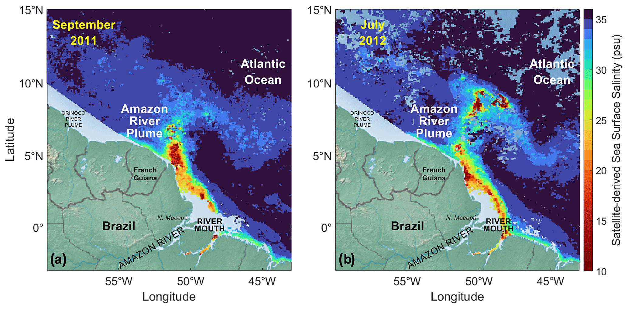
Figure 1Sea surface salinity (SSS) for the Amazon River plume (15∘ N–3∘ S, 43–60∘ W) during (a) September 2011 and (b) July 2012, derived from a remotely sensed diffuse attenuation coefficient at 490 nm. Area likely affected by the Orinoco River plume (<150 km off the coastline between 55–60∘ W) is excluded from this study. Oceanic regions in light blue on the maps indicate that the satellite-derived SSS data are unavailable, mostly due to muddy nearshore waters or clouds. See Mu et al. (2021) for further details.
In this study of hypothetical alkalinity addition at the Amazon River mouth, we investigate the expected changes in air–sea CO2 flux at the offshore Amazon plume waters and examine what perturbation size and sampling density would be needed to measure the alkalinity change and verify a resultant anomalous CO2 flux. We make use of the knowledge from previous field studies of the carbonate chemistry in the Amazon River plume to address two main goals: (1) analyze the potential for detectability of OAE-induced alkalinity change relative to measurement precision, background variability, and sample size and (2) estimate changes in ocean pCO2 and air–sea CO2 flux in the Amazon River plume due to hypothetical alkalinity addition at the river mouth. Our effort aims to outline how one might consider the measurement, reporting, and verification (MRV) needed in the context of known background variability. We argue that this kind of sensitivity analysis is a first step that could lead to more realistic numerical simulations if the system does not fail basic tests of feasibility.
2.1 Study site and mixing model
We use a river–ocean conservative mixing model (Cooley and Yager, 2006) informed by direct observations collected as parts of the ANACONDAS (Amazon iNfluence on the Atlantic: CarbOn export from Nitrogen fixation by DiAtom Symbioses) and ROCA (River Ocean Continuum of the Amazon) projects (Mu et al., 2021, 2023) to establish expectations of how alkalinity perturbations would influence the carbonate system in the Amazon plume (the gray and green pathways on the methods schematic shown in Fig. 2). The mixing model assumes no sources or sinks of the carbonate species modeled, and the deviations from this assumption are discussed in Sect. 2.2. In this model, dissolved inorganic carbon (DIC) and total alkalinity (TA) are treated as conservative tracers and used to describe pCO2 variations as a function of salinity and temperature (Fig. 1). TA and DIC can be, respectively, expressed as
We adopt the explicitly conservative form of TA here (Wolf-Gladrow et al., 2007) so that TA changes due to the addition of our hypothetical calcium-based alkalinity feedstock can be fully tracked by the increase in calcium ion concentration. To establish the baseline condition of the carbonate system in the Amazon River–ocean continuum, we adopted the river endmembers from Mu et al. (2023; also Table 1) and ocean endmembers (S=36, TA=2369 µmol kg−1, DIC=2025 µmol kg−1) from Mu et al. (2021). The conservative mixing model can be further expressed as
SSSmix is the salinity for a plume sample, Sr is the salinity of the river endmember (Sr=0), and SSSo is the surface salinity of the ocean endmember. In Eq. (4), fr and fo are the proportions of river and ocean in the sample, both of which can be solved when SSSmix is known. The theoretical TA and DIC in the plume, TAmix, and DICmix at any given SSSmix are then calculated from the known endmember properties and proportions via
Eventually, pCO2mix and pHmix at a given salinity and observed temperature are calculated with CO2SYS (Lewis et al., 1998) from inputs of TAmix and DICmix. In this calculation we use the carbonic acid dissociation constants K1 and K2 from Millero (2010) due to their eligibility across a wide salinity range suitable for this study.
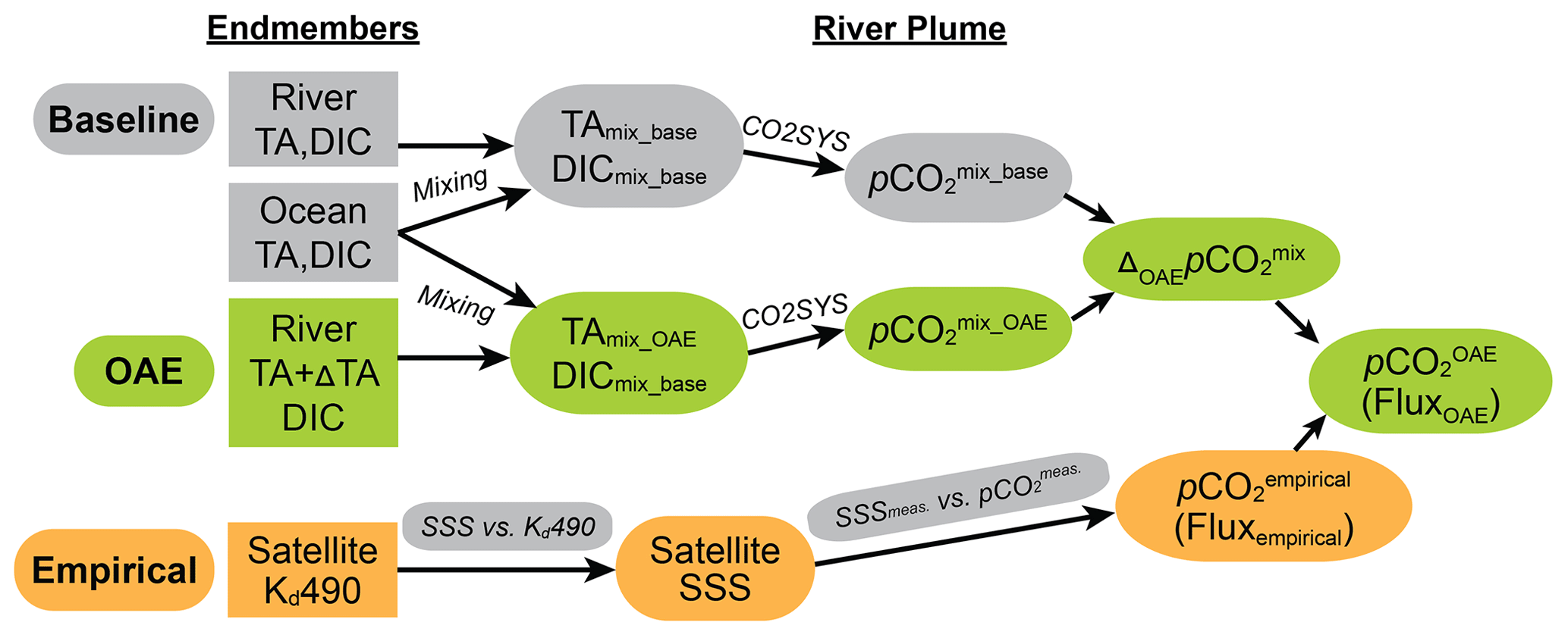
Figure 2Schematic diagram for the method used to calculate carbonate chemistry and air–sea CO2 fluxes before and after a hypothetical alkalinity addition (OAE) in the Amazon River–ocean continuum. The baseline and OAE pathways (gray and green) use the conservative mixing model (Eqs. 3–6) and CO2SYS to calculate the baseline and hypothetical OAE pCO2. The difference between the baseline and OAE mixed models () is added to the empirically derived pCO2 at every SSS. The resulting is used to calculate the air–sea CO2 flux across the surface of the plume for each hypothetical OAE experiment.
Table 1Baseline total alkalinity (µmol kg−1) determined at the N. Macapá gateway at the Amazon River mouth during September 2011 and July 2012 (Mu et al., 2023). The means represent the river's alkalinity endmember in that month.
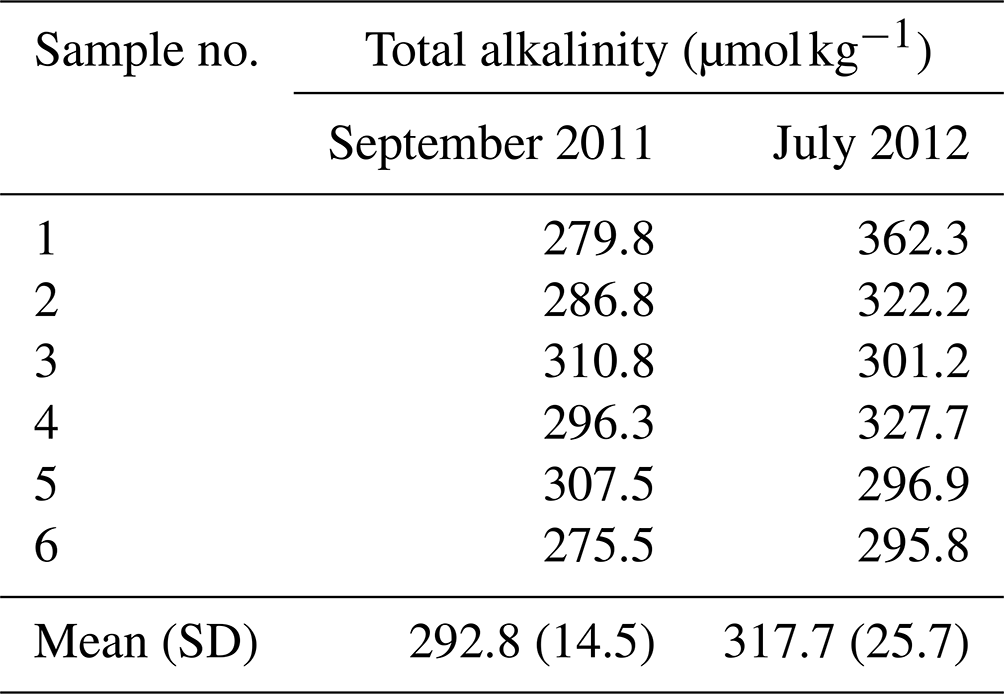
We confined our study periods to two specific months, September 2011 and July 2012, during which measurements were made in both the river and throughout the Amazon River plume. During the river plume expeditions, surface seawater pCO2, temperature, salinity, and chlorophyll fluorescence were continuously measured shipboard across the Amazon-influenced regions. An oceanic station was specifically sampled for TA and DIC during each cruise as the ocean carbonate endmember for each corresponding month (Mu et al., 2021). Details in quantifying the river endmembers are described in Ward et al. (2015) and Mu et al. (2023). Briefly, the Amazon River mouth region receives freshwater runoff from three channels: the north and south channels near Macapá and the channel of the Tocantins River near Belém (Fig. S2 in the Supplement). Sampling was conducted at the lower reaches of the three channels near the mouth (or “gateways”) in each month. Six TA and DIC samples were collected at three cross-channel locations of each gateway (left bank, center, and right bank) from both the surface and 50 % depth (5–10 m). For a concise demonstration on the detectability of the alkalinity addition in the river, we chose to target one gateway (North Macapá) as the perturbation site and consider how many samples would be needed to observe the TA perturbation relative to that gateway's background variability. However, to quantify the potential CDR induced by a TA perturbation just above detectability, we assumed the entire river mouth would be perturbed equally as in North Macapá. Because the outflow through both North and South Macapá gateways comprises >80 % of total discharge (Ward et al., 2015; Mu et al., 2023) and their chemical properties are almost identical seasonally (Mu et al., 2023), North Macapá is representative of the mouth's chemical composition. In an actual OAE field trial, perturbing one gateway will perturb the mouth region by an amount proportional to the percentage discharge there (relative to the combined discharge), and the natural variability in the unperturbed gateways will affect the background variability at the mouth. There are key unknowns in seasonal TA contributions from other gateways to the mouth which prevent us from combining all the gateways. Therefore, the mean and standard deviation of the six TA values at North Macapá, respectively, were then used as the river TA endmember and its natural background variability (Table 1).
2.2 Deviations from the conservative mixing model
The assumption that TA and DIC act as conservative tracers is not true in the presence of photosynthesis, respiration, bio-calcification, abiotic dissolution/precipitation of calcium carbonate, and/or air–sea gas exchange. In fact, plume pCO2 values measured from an underway system on the research vessels surveying for the ANACONDAS program were systematically lower than predicted from the mixing model (Mu et al., 2021; Fig. S3 in the Supplement). This offset was assumed to be due to net community production, an assumption supported by the strong correlation between shipboard chlorophyll and the difference between the pCO2mix calculated from conservative mixing and the measured pCO2 (Mu et al., 2021).
A linear regression between measured SSS () and measured pCO2 showed a strong linear relationship (r=0.79 for September 2011 and r=0.97 for July 2012). Therefore, we use SSS to calculate an empirical estimate of pCO2 (pCO2empirical) at every SSS level in each month (orange pathway in the schematic shown as Fig. 2). SSS fields in the Amazon plume were derived from the remotely sensed diffuse attenuation coefficient at 490 nm (Kd490, Fig. 1). The measured SSS vs. pCO2empirical regression is used to map pCO2empirical at every satellite-derived SSS value in the plume (as in Fig. 3a) and to calculate the empirical air–sea CO2 flux, according to the following equation:
where k is the gas exchange coefficient calculated from gridded reanalysis wind speed and the parameterization of Sweeney et al. (2007), α is the solubility of CO2 in seawater (a function of water temperature and salinity, calculated from equations in Weiss, 1974), and pCO2atm is the monthly averaged pCO2 in the atmosphere measured at a nearby NOAA monitoring station. Details in calculating the empirical CO2 flux can be found in Mu et al. (2021).
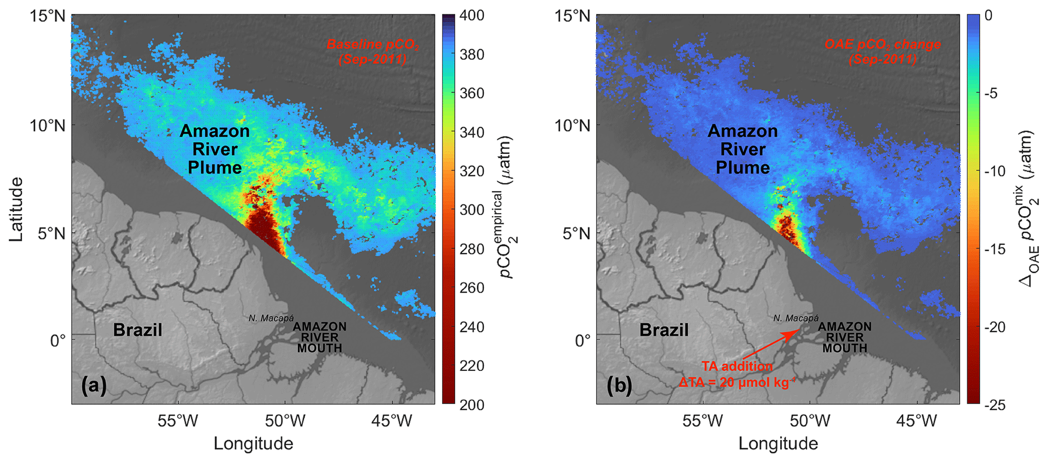
Figure 3pCO2 at the surface of the Amazon River plume and its predicted response to alkalinity addition based on satellite-derived SSS. (a) Spatial distribution of unperturbed pCO2empirical (µatm) at the surface of the Amazon River plume () during September 2011, with SSS outside of the plume range removed from this map as the remotely sensed Kd490 vs. SSS regression is sufficiently robust only when (see Fig. 2 and Sect. 2.2 for details on how the mapped quantity is defined and Mu et al., 2021, for additional details). (b) Predicted changes in the plume surface pCO2 (i.e., ΔOAEpCO2mix from Eq. 8) due to addition of 20 µmol kg−1 of alkalinity at the Amazon River mouth during September 2011.
2.3 Experimental design
The core of this sensitivity analysis is to manipulate the concentrations of TA at the river mouth by the addition of a hypothetical alkalinity feedstock. There are several feedstocks that could be considered for this purpose, each with a distinct set of considerations (Hartmann et al., 2013; Renforth and Henderson, 2017). Magnesium- or silicate-rich rocks such as olivine and other basalts (Hartmann et al., 2013), carbonate minerals (e.g., Rau, 2011; Renforth et al., 2022), mineral derivatives found in some industrial waste products, or even electrochemical production of alkalinity (Tyka et al., 2022; He and Tyka, 2023) are all candidates (NASEM, 2021). The stoichiometry of the reaction, dissolution rate, risk of secondary precipitation, and contamination with metals are all specific to the particular alkalinity source chosen. Quicklime (CaO) has been identified as being promising due to its high solubility in seawater and rapid dissolution rates (Kheshgi, 1995; Moras et al., 2022). Quicklime is made by heating limestone (primarily CaCO3), an abundant rock at the Earth's surface. The heating of each molecule of CaCO3 releases one molecule of quicklime and one molecule of CO2 (Kheshgi, 1995). Therefore, carbon capture and storage of the released CO2 would be necessary for OAE to be effective from the application of quicklime (Paquay and Zeebe, 2013; Renforth et al., 2013; NASEM, 2021; Moras et al., 2022). Hereafter, we assume that the alkalinity feedstock for the hypothetical OAE deployment is quicklime, which simplifies the discussion of stoichiometry, precludes contamination from metals and other industrial contaminants, justifies our assumption of rapid dissolution, and informs our discussion of potential unintended consequences.
Assuming the additional CaO converts 100 % to TA according to stoichiometry, the dissolution of CaO consumes CO2 and releases through
For every mole of additional CaO, TA is increased by 2 mol (Eq. 1), while DIC remains constant (i.e., consuming 2 mol of CO2 while producing 2 mol of bicarbonate in Eq. R1) before any significant air–sea equilibration occurs. This assumption of a constant DIC during perturbation should hold over the timescale of the river–ocean mixing based on the following evidence: (1) CaO dissolution happens on hour scales (Moras et al., 2022), and (2) the time elapsed between the river outflow at the mouth and its mixing with ocean to relatively high salinity (SSS>15) is as short as 2 weeks (see Fig. 5 from Coles et al., 2013), while the air–sea CO2 equilibration usually takes several weeks to months in the western tropical North Atlantic (Jones et al., 2014). We assume in this study that there is no secondary precipitation of CaCO3 and that the additional CaO stays at the surface layer until fully dissolved. Another underlying assumption is that CaO is homogeneously mixed across the river mouth gateway, eliminating potential uncertainty/variability due to patchiness of the TA addition. We will address key unknowns associated with these assumptions in the Discussion.
We explore TA perturbations over the range 1–100 µmol kg−1 (i.e., perturbation between 0.07 and 7 times the natural variability for September 2011 and 0.04 and 4 times the natural variability for July 2012). The mixing model is recalculated with each of the perturbed river endmembers to find the perturbed TAmix and DICmix across the plume. We then use CO2SYS to calculate the theoretical pCO2mix_OAE at each salinity stamp with the perturbed TAmix, DICmix, and observed temperature as inputs to compare to the unperturbed baseline. The difference of the TA-enhanced seawater pCO2 and the baseline pCO2 is
In each perturbation scenario, the added alkalinity lowers the pCO2mix_OAE below the unperturbed mixing curve by the amount of ΔOAEpCO2mix. To finally arrive at the surface ocean pCO2 needed to calculate the air–sea fluxes according to Eq. (7), we add the ΔOAEpCO2mix to pCO2empirical:
This approach (schematized in Fig. 2) implicitly assumes that the biological processes that lower the measured pCO2empirical below the theoretical pCO2mix would be unchanged from the deployment of additional alkalinity, an assumption that would demand careful testing in the field.
2.4 Sensitivity evaluation for detectability of hypothetical OAE deployments
To assess the TA detectability, we evaluate perturbations in one river gateway (North Macapá). We use a simple bootstrapping technique (or Monte Carlo simulation) to assess the minimum TA perturbation that would be detectable with a given number of measurements, taking into consideration the background variability during a given season and reasonable measurement precision.
We randomly generate 1000 baseline TA values under a normal distribution using the mean and standard deviation of the six measured TA values in September 2011 or July 2012. We then generate 1000 perturbed TA values for each perturbation scenario under a normal distribution, where the mean is the addition of the baseline mean and the perturbation strength, with the same standard deviation as the baseline. The range for the tested perturbation sizes is 1–20 µmol kg−1 of TA. Within the 1000 TA pools from both the baseline and a perturbation scenario, we randomly select 1–100 values (i.e., varying sample size) from both pools, perform the student's t test between the selected sets, and calculate the p value to determine if the perturbed TA set would be seen as significantly different from baseline. The t test is repeated 200 times for each perturbation size and sample size, generating 200 p values. The mean of those p values is calculated for each perturbation scenario at each sample size (Fig. 4). A lower p value suggests a higher likelihood that the perturbed TA values would be considered significantly different from the baseline and therefore “detectable”. We use a threshold of p<0.1 to indicate statistical significance.

Figure 4Detectability of hypothetical TA enhancement relative to background variability. (a and b) The theoretical shift of TA (µmol kg−1) means and distributions for September 2011 and July 2012 due to the addition of 20 µmol kg−1 of TA at the Amazon River mouth. Black lines indicate the in situ TA measurements at the mouth on which the baseline data distributions are based. The standard deviations in the perturbation scenarios are assumed the same as those from the baseline. (c and d) The p-value maps from t tests performed between the baseline and TA perturbation scenarios at various sample sizes and TA perturbation strengths for September 2011 and July 2012. Areas in yellow (p<0.1) indicate conditions where an analyst would conclude that the TA perturbation was detected relative to the baseline condition with 90 % certainty.
3.1 Baseline carbon chemistry in the plume
The surface pCO2empirical in the Amazon River plume derived from remotely sensed SSS generally ranged from 210–400 µatm in September 2011 (Fig. 3a), with the lowest values in low-salinity regions near the French Guiana coast, which increase as the river mixes with ocean water (Fig. 1a). Figure 3a masks out regions with surface salinity below 15 and beyond 35 psu, as these waters are out of the range of a sufficiently robust algorithm between Kd490 and SSS (Mu et al., 2021).
The distribution of plume surface pCO2sw is primarily shaped by two processes: the Amazon River–ocean mixing and biological CO2 consumption/release in the plume waters (Mu et al., 2021). For example, zero-salinity river water near the mouth is supersaturated with respect to atmospheric CO2 in July 2012, where pCO2>1000 µatm is observed (Mu et al., 2021, 2023) due to low carbonate buffer capacity and high microbial respiration. As the river waters mix with the ocean, the sharp increase in buffer capacity and shift towards a net autotrophic state lowers the surface pCO2 towards a minimum (below pCO2atm in July 2012; Mu et al., 2021) before rising towards the open ocean levels closer to equilibrium with the atmosphere (i.e., pCO2∼400 µatm) at higher salinity (Fig. S3). The nitrogen-fixing diatom–diazotroph assemblages and other phytoplankton that are active in the Amazon plume waters (Goes et al., 2014) further enhance the CO2 undersaturation in mid- to mid-high-salinity portions of the plume (i.e., ) on top of the undersaturated CO2 state caused by conservative mixing (Mu et al., 2021).
3.2 Detectability of TA perturbations
We propose that the minimum requirement for MRV in a watershed OAE experiment is that the perturbed TA in the river can be detected above background variability. To illustrate the challenge of detectability, we consider the background TA variability in the North Macapá gateway in September 2011, with the assumption that the variability measured at that time (standard deviation of 14.5 µmol kg−1) is representative of that season and gateway. It is intuitive that a large enough perturbation (commensurate with the standard deviation) is detectable with a small number of samples (Fig. 4), and a small perturbation (a factor of 3 smaller than the standard deviation or smaller) cannot be detected against the background variability regardless of the number of samples. This exercise reveals the challenge of balancing the effort needed to detect the perturbation against the obstacle and risk of increasing the TA by a large amount.
As expected and illustrated in Fig. 4, higher sample sizes and TA perturbations lead to greater detectability of the alkalinity enhancement. For practical purposes, neither sample size nor perturbation strength can be increased infinitely, so OAE experiments would likely seek a balance between the two. For example, in September 2011 (Fig. 4a and c), a TA perturbation of ∼7–10 µmol kg−1 at a background standard deviation of 14.5 µmol kg−1 would have been readily detectable with 40 samples. For July 2012 (Fig. 4b and d), when background variability was higher (25.7 µmol kg−1), 40 samples would detect perturbations only if they were to exceed +20 µmol kg−1 of TA. In an actual field OAE trial, each season (and gateway) may have different background variability that would require measurement and characterization in advance of any perturbation to have a clear strategy for sampling.
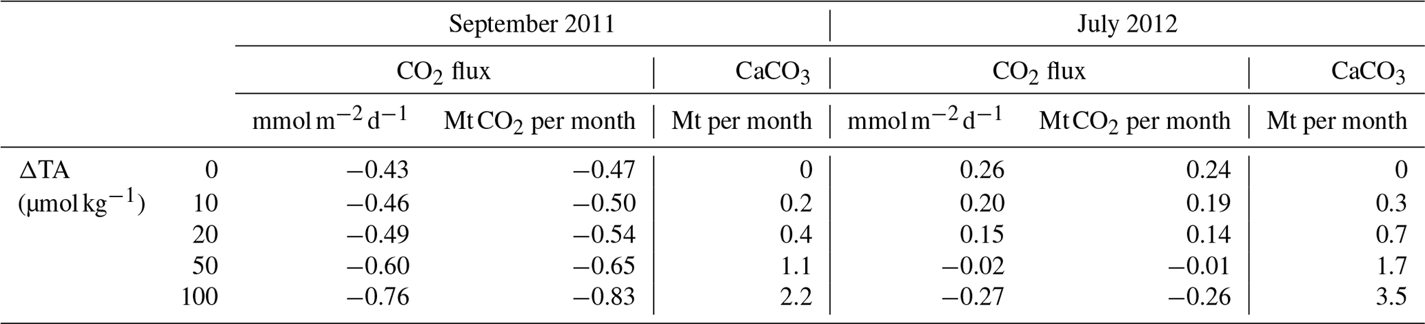
Table 2Summary table for air–sea CO2 flux in the Amazon River plume () and the mass of CaCO3 mineral required for each TA perturbation size (ΔTA) in each month. Positive fluxes indicate CO2 outgassing, and negative fluxes (–) indicate ocean CO2 uptake. Note that the post-perturbation CO2 flux and CaCO3 demand increase linearly with increase in ΔTA.
3.3 Impact on pCO2 and air–sea CO2 flux
Figure 3b shows the pCO2mix decrease due to a hypothetical TA addition in the Amazon watershed, which is highest in the low-salinity waters near the river mouth and attenuates at higher salinities due to mixing with the unperturbed ocean water. Figure 5 provides a quantification of the air–sea CO2 flux at each salinity level for different TA perturbation strengths (20, 50, and 100 µmol kg−1). While the air–sea CO2 flux per unit area (or flux density) is greatest at low salinities (Fig. 5a and b), the large area occupied by the diluted plume (salinities greater than 32; Fig. S4 in the Supplement) means that more than half of the total integrated air–sea CO2 exchange – as well as the perturbation to this flux – would occur in this salty part of the plume.
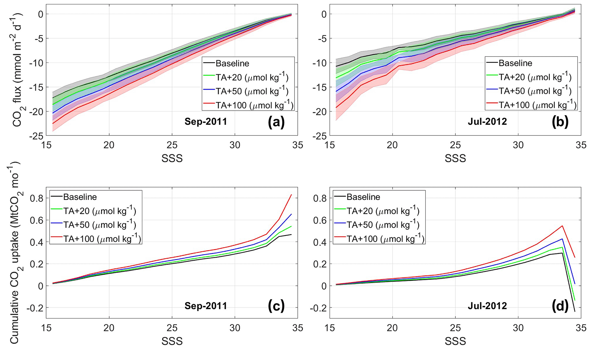
Figure 5The impact of TA addition on ocean uptake of CO2 across the Amazon River plume. (a and b) Air–sea CO2 flux density () in the Amazon River plume at different sea surface salinities for the baseline and multiple TA perturbation scenarios in (a) September 2011 and (b) July 2012. Standard deviations of the fluxes within each salinity band (1 psu apart) are represented by the shaded areas. Negative values indicate atmospheric CO2 sinks. (c and d) Cumulative ocean CO2 uptake (Mt CO2 per month) in the Amazon plume due to TA additions in (c) September 2011 and (d) July 2012. SSS ranging between 15 and 35 is used, while SSS<15 and >35 is omitted because the remotely sensed Kd490 vs. SSS regression is sufficiently robust only when according to the Amazon River plume definition from Mu et al. (2021).
Air–sea CO2 exchange at SSS=34–35 for July 2012 is only slightly greater than 0 (Fig. 5b), but due to the large area of plume at near-oceanic salinity level, the total plume CO2 uptake (i.e., negative flux) in lower S regions is entirely offset by the CO2 outgassing at . Regardless of whether the baseline Amazon plume is a carbon sink or source, the change in air–sea CO2 exchange due to OAE shifts toward more carbon storage by the ocean and increases linearly with the size of TA perturbation (Table 2).
4.1 Unaccounted for plume region with great CDR potential
While we explored the OAE-induced additionality of the carbon uptake (or net CDR) at different salinities in the Amazon River plume (Fig. 5), it is important to note that the cumulative additional uptake in Fig. 5b excludes the freshest part of the plume (SSS<15). Due to high organic carbon remineralization in shallow waters (Mu et al., 2021), the quasi-linear SSS versus pCO2 empirical relationship collapses at SSS<15 and prevents the establishment of empirical pCO2 in this region. Therefore, we excluded SSS<15 in our analyses (e.g., in Fig. 3, coastal areas <50 m deep near the mouth are masked) while acknowledging that because of the strong CO2 outgassing in this region, the baseline air–sea CO2 flux in the entire plume () will be shifted towards more CO2 release, should the SSS<15 water be included. However, once TA is added, surface pCO2 will decline in the entire plume regardless of salinity, causing greater net CO2 drawdown across the plume. In other words, the OAE-induced CO2 uptake increase calculated for plume water could substantially underestimate the true additionality when SSS<15 is not considered. The area of the S<15 water is small compared to the plume (i.e., <15 % of the SSS>15 plume area), but its lower buffer capacity also means pCO2 is much more sensitive to TA addition, and therefore could still contribute a considerable amount to CDR.
A basic scaling would suggest that 10 % of the plume area with an OAE-induced surface pCO2 decrease of 30 µatm would have as large an impact on area-integrated ocean uptake as the portion of the plume with a 3 µatm decrease. Therefore, including the freshest part of the plume and calculating its reduction in outgassing could easily double our estimate of additional CO2 uptake for the entire plume. Lacking both knowledge of the spatial distribution of salinity and a robust estimate for pCO2 in this low-salinity region prevents us from quantifying its CDR potential in a rigorous manner.
However, we can still conduct a back of the envelope calculation to estimate the distribution of CDR between SSS<15 and regions of the plume. With an addition of 20 µmol kg−1 TA and an averaged Amazon freshwater discharge of 0.18 Sv (Fig. S1), we can calculate the total transport of this TA addition of 9.3×10⁹ mol per month. Given sufficient time for air–sea re-equilibration and the subsequent DIC increase due to OAE, we can assume the maximum DIC increase would be 0.8 times the ΔTA (Wang et al., 2022). Therefore the maximum CDR resulting from TA addition would be mol per month, or 0.3 Mt CO2 per month. Given that the estimated enhanced CO2 flux in the S>15 region is approximately 0.07–0.1 Mt CO2 per month (Table 2), ∼0.2 Mt of CO2 uptake per month would be expected to take place in the low-salinity region (SSS<15), which is consistent with the estimation based on direct air–sea CO2 flux change. This calculation highlights the potentially important role of the freshest part of the plume in the net CDR by the entire plume, which could be disproportionately large relative to its small size.
4.2 Exploring the minimum TA detectability
Here we propose that the minimum MRV requirement for an OAE experiment in a river be that the TA increase can be detected in the fresh river endmember, and we showed what size perturbation and sampling density would meet that minimum for the Amazon River. We found that the minimum detectable TA addition at the Amazon River mouth ranges between 10–20 µmol kg−1, with a reasonable sample size of 40 during field campaigns before and during the perturbation (Fig. 4c and d). We focus on detectability results for TA, since that is the variable directly targeted by any OAE approach. However, we present similar detectability analyses for the increase in pH (Fig. S5 in the Supplement) and decrease in pCO2 in the river mouth (Fig. S6 in the Supplement), which shows that the perturbation to these variables from a 10–20 µmol kg−1 is also readily detectable with a reasonable number of samples. With commercially available autonomous sensors for pH and pCO2 (Kapsenberg et al., 2017; Sabine et al., 2020), these might be attractive proxies for the added TA.
One may further hope that MRV efforts for OAE deployed at the river mouth would document reductions in plume pCO2. We rely on the observed pCO2, a mixing model, and satellite-derived SSS to deduce where one might expect pCO2 reductions to be measurable relative to background concentrations. Sensors for measuring aboard ships and uncrewed surface vehicles like Saildrone and Waveglider have a target accuracy of 2 µatm (Sabine et al., 2020). Figure 3 shows that, if Amazon River water TA was continuously increased by 20 µmol kg−1, a broad region of the plume would see pCO2sw decreases measurable with current sensor technology if they could sustain regular sampling over the SSS<30 region before, during, and after the OAE deployment.
However, like with the detectability of the TA in the river mouth, the pCO2 perturbation must be detectable given background variability and does not depend only on sensor accuracy. Here, a measure of that background variability is the root mean square error (RMSE) between the pCO2empirical, calculated from the linear regression of the in situ observations of pCO2 and SSS, and the actual observations of pCO2 (pCO2measured, Fig. 2). For September 2011, the rms error of this regression is ∼22 µatm for (Fig. S7 in the Supplement). Thus, we would expect that a perturbation approximately this size would be detectable with sufficient samples at the river mouth (Fig. S6). Figures 3 and S7 suggest that a region of the plume near the river mouth approximately could meet this criterion due to (1) lower salinity and higher perturbed TA and (2) relatively lower rms error in pCO2empirical and thus low background pCO2 variability. This speculation is nicely verified in a minimum OAE detectability test using pCO2 in the plume waters as the proxy (Fig. S8 in the Supplement), where the reduction in pCO2 at is readily detectable with 10 samples for waters (Fig. S8c), contrasting sharply with the poor detectability at higher salinity (; Fig. S8d).
It is encouraging that SSS can be estimated from satellite measurements, allowing for field campaigns – including uncrewed vehicles piloted from operators onshore – to find and sample in the plume where an OAE-induced pCO2 reduction may be detected. Nevertheless, Fig. 5 shows that nearly half the additional ocean CO2 uptake due to the OAE experiment could happen in the part of the plume with , where detecting the perturbation in TA and plume surface pCO2 is impossible with the accuracy of existing sensors or the laboratory analysis of bottle measurements.
Finally, we consider the amount of limestone (CaCO3) required to produce pulverized quicklime as the alkalinity source material that sustains a set TA perturbation size (Table 2). The limestone equivalents needed to create a detectable perturbation of +20 µmol kg−1 of TA is 0.4 Mt per month using river discharge numbers from September 2011, which is approximately equal to 0.04 % of US industrial limestone production in the year 2021 (USGS, https://pubs.usgs.gov/periodicals/mcs2021/mcs2021-stone-crushed.pdf, last access: 24 May 2023). Using river discharge for July 2012, the requirement grows to 0.7 Mt limestone per month. In terms of OAE-induced additional CO2 uptake, every 0.1 Mt CO2 per month represents more than 30 times greater CDR than the CO2 captured by one ORCA Direct Air Capture plant in a full year (https://en.wikipedia.org/wiki/Orca_(carbon_capture_plant), last access: 24 May 2023), yet amounts to less than what Brazil emitted on an average 2 h basis in 2021 (https://www.icos-cp.eu/science-and-impact/global-carbon-budget/2021, last access: 24 May 2023). It is worth noting that concerns have been raised over the feasibility of CaO liming considering the energy need and CO2 release associated with the production of this alkalinity source (e.g., Paquay and Zeebe, 2013; Renforth et al., 2013; Voosen, 2022), but limestone calcination coupled with heat recovery and carbon capture and storage technologies is found to significantly reduce energy costs and CO2 emission during CaO production, potentially making this liming approach more sustainable (Foteinis et al., 2022).
4.3 Constraints on OAE deployments
So far, we have focused most of our efforts on describing the minimum detectable OAE perturbation. It is also important to consider what might constrain the upper limit of TA addition (i.e., through liming), such as ecosystem disturbances and secondary precipitation of calcium carbonate. Ideally, OAE would not put the ambient marine ecosystems at risk. The minimum detectable perturbation described above is close to the background TA variability and so has a greater likelihood for a small impact on the ecosystem relative to larger deployments. Heavy metals in some source alkaline minerals are problematic (NASEM, 2021), a consideration avoided with the use of a 100 % pure CaO compound as the source of TA addition. The highest perturbation we explored was +100 µmol kg−1 of TA added to the river endmember, which would lead to initial pH increase of 2.0 at the river mouth, a pCO2sw decrease of up to 100 µatm (data not shown) in the Amazon plume, and a total enhanced atmospheric carbon uptake of ∼0.35 Mt CO2 per month across the plume (, with considerable additional contribution likely in the freshest plume waters) during September 2011 (Table 2 and Fig. 5c). This level of initial pH increase at the TA addition site is likely concerning for local marine communities, although the effect would be dispersed by the river and diminish with increasing distance from the river due to mixing.
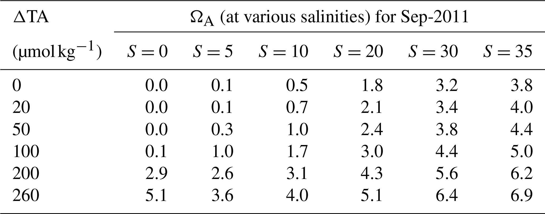
Another constraint on the upper limit of TA addition through ocean liming is secondary CaCO3 precipitation and the resulting reduction of atmospheric CO2 uptake. Moras et al. (2022) suggested that runaway CaCO3 during OAE may be avoidable if the saturation state of aragonite (ΩA) is kept below 5 for natural seawater. Assuming such a ΩA threshold for barely avoiding CaCO3 precipitation is also applicable in fresher Amazon plume and river water, we have calculated the corresponding maximum TA perturbation allowed to keep ΩA below this threshold according to the method in Mucci (1983), with the results shown in Table 3. Because the ΩA increases with salinity, TA perturbation that likely avoids secondary CaCO3 precipitation becomes substantially smaller close to SSS=35 (i.e., ∼100 µmol kg−1, compared to ∼260 µmol kg−1 at S=0). Adding 20 µmol kg−1 of TA in September 2011 would only increase ΩA by a maximum of 0.3 (Table 3), and ΩA stays below 5 everywhere in the plume for TA additions of 100 µmol kg−1 or smaller. An important caveat on assuming a ΩA threshold of 5 is that the Amazon River at the mouth contains heavy loads of mineral particles and will likely facilitate the formation of heterogeneous nucleation and precipitation for CaCO3 (Renforth and Henderson, 2017; Moras et al., 2022), thereby lowering the maximum TA addition allowed. Further study is needed to ensure ΩA is always kept below the proper precipitation threshold in all regions of the river plume.
Table 3Theoretical aragonite saturation state (ΩA) for different TA perturbation strengths (ΔTA) and salinity levels at the surface of the Amazon River and its plume during September 2011, according to the equation . [Ca2+] is calculated by adding the increment of [Ca2+] due to TA perturbation (i.e., ) to the unperturbed [Ca2+]. The unperturbed [Ca2+] term is comprised of relative contributions from both the river and ocean [Ca2+] endmembers at a specific salinity. [Ca2+] of 0.15 mmol kg−1 is used as the river endmember, approximating results from Drake et al. (2021), and the global ocean average [Ca2+] of 10.28 mmol kg−1 is used as the ocean endmember. [] is derived from theoretical TA and DIC in the river–ocean endmember mixing model (see Sect. 2.1 and Fig. 2) using a constant water temperature of 29 ∘C (or 302.15 K). The temperature- and salinity-dependent stoichiometric solubility product for aragonite, , is calculated from Mucci (1983). The following equations in Mucci (1983) are involved in the determination of for each salinity: and ; SSTK is the sea surface temperature in Kelvin (i.e., SSTK=302.15 K); and b, c, and d are constants reported in Mucci (1983).
Adding TA to the land surrounding the Amazon watershed could have possible advantages over spreading across the open ocean, involving co-benefits to the terrestrial ecosystems and agriculture such as increased crop yield in agricultural watersheds (Caires et al., 2006; Hartmann et al., 2013; Beerling et al., 2020), reduced soil runoff (Taylor et al., 2016), and reduction of N2O production (Beerling et al., 2018). Introducing the TA on land might also slow its dissolution in the river and allow its reaction with CO2 to form bicarbonate in pore water, helping reduce the risks associated with large perturbations to pH and TA, like secondary precipitation or phytoplankton community perturbations. Basaltic rock with slower dissolution rates, but more favorable stoichiometry from CDR than carbonates (Beerling et al., 2018), might also provide an alternative TA feedstock for land-based deployment. However, deployment on land would likely increase the difficulty to quantify the effect of TA addition for MRV purposes.
4.4 Additional challenges
One of the underlying assumptions for this analysis is that CaO reacting with CO2 takes place in a time frame faster than air–sea re-equilibration takes to occur, and the layer of plume water dwells at the surface for a relatively long period of time. If the TA-enhanced surface plume is not exposed to the atmosphere long enough to allow for full air–sea CO2 equilibration (e.g., due to water mass subduction), CO2 removal efficiency will decrease in these regions (Jones et al., 2014). A logical next step to characterize the spatial footprint of the hypothetical experiment and the total timescale for equilibration would be to simulate the time-evolving patch of the alkalinity anomaly, the corresponding pCO2 perturbation, and the total excess DIC in an ocean general circulation model with the OAE experiment relative to a control simulation.
We argue that the TA-enhanced waters do not need to remain continuously within the surface layer to induce ocean CDR. The change in the air–sea flux can be realized whenever the perturbed waters influence the surface, even if that is far from the plume or years after the deployment. Though the implied dilution of the signal or delay in causing additionality of the CDR may not change the net impact of the OAE experiment if integrated over a sufficiently long time period, it would make MRV of the total impact essentially impossible through observational methods alone.
Another assumption in this work was that photosynthesis, which is known to drive pCO2 beneath the conservative mixing curve (Mu et al., 2021), would be unchanged by the alkalinity addition. This assumption is premised on the argument that perturbations barely detectable above background variability are unlikely to strongly change the ambient ecosystem, an argument supported by a number of recent studies. For example, results from a mesocosm experiment with Tasmanian coastal waters show statistically significant, though relatively moderate, changes to phytoplankton community structure and function at high TA perturbation values of +495 µmol kg−1, which are 25 times higher than the minimum detectable perturbation explored here (Ferderer et al., 2022). Another microcosm incubation study reveals the alkalinity enhancement inducing minor but largely negligible short-term effects on primary productivity and no measurable changes in biological CaCO3 precipitation, even at a TA perturbation level of +2000 µmol kg−1 (Subhas et al., 2022). Regardless, ecosystem impacts would require careful monitoring in any field OAE experiment.
If the alkalinity source for OAE is quicklime, managing the heat released through its exothermic reaction during dissolution in water at a rate of 64 kJ mol−1 CaO is another important consideration. Taking the highest perturbation scenario explored in Table 2 that increases TA in the Amazon watershed by 100 µmol kg−1, we estimate 310 MW total heat released during the duration of the dissolution. In order for the heat released from the CaO reaction to be lower than 10 % of the daily solar radiation at the Equator ∼400 W m−2 (a level that would presumably be swamped by natural variability in the river's heat budget), the TA injection would have to occur over an area of river larger than about 8 km2, e.g., 2 km of river width and 4 km along its length. Therefore, it is possible to minimize the environmental risk due to heat released during quicklime dissolution by spreading it over a large enough area at the river mouth.
We conduct a sensitivity analysis of alkalinity enhancement in the Amazon River watershed, evaluating the detectability of added TA and predicting its influence on the atmospheric CO2 uptake in the offshore plume. Adding 20 µmol kg−1 of TA in a month at the Amazon watershed could increase the CO2 uptake by the river plume by at least 0.07–0.1 Mt CO2 per month. The full CDR might be as much as 3 times as high as this estimate due to reduced outgassing in the freshest part of the plume, where we lack a robust empirical pCO2sw–salinity relationship and therefore cannot robustly quantify the anomalous air–sea exchange in this region. We found that a TA perturbation of +10–20 µmol kg−1 in the river is readily detectable with at least 40 samples, given the background variability of 15–30 µmol kg−1. By adding a TA perturbation barely detectable relative to the background TA variability, the likelihood of substantial environmental disturbance at the injection site would be minimized. However, observing the corresponding pCO2 perturbation in the plume presents a greater observational challenge. Even with the highly sensitive pCO2 sensors available today (e.g., Sabine et al., 2020), detectability of the pCO2 anomaly is plausible only in the fresher part of the plume given the dilution of the signal at higher salinities and large background variability. Quantifying the total additional CO2 uptake from this type of OAE cannot rely on observations alone; idealized conceptual models like the one presented here and more sophisticated circulation-biogeochemical ocean models will always be required to understand the total CDR because the additional CO2 uptake is likely to occur over long time periods and at very diluted perturbation levels. It is also clear that the basic scientific feasibility we aimed to assess here does not reveal the full feasibility of such interventions: ocean-based CDR research and deployment require care and attention to ethical, political, and governance issues.
Data for the air–sea CO2 flux calculations in the Amazon River plume are from Mu et al. (2021). The river mouth data are reported in a manuscript currently under revision in Global Biogeochemical Cycles that will be resubmitted in May 2023. All codes are available at https://drive.google.com/drive/folders/1YYjcT5ZYvyHoJaKmRl3Fd8aagMhtRwCA?usp=share_link (last access: 16 May 2023).
The supplement related to this article is available online at: https://doi.org/10.5194/bg-20-1963-2023-supplement.
JBP and LM conceptualized the framework of this experiment. LM, JBP, and HW designed the methodology. LM performed the analytical calculations and numerical simulations. LM wrote the paper with support from JBP and HW. JBP supervised the project.
The contact author has declared that none of the authors has any competing interests.
Publisher's note: Copernicus Publications remains neutral with regard to jurisdictional claims in published maps and institutional affiliations.
We would like to thank Patricia Yager for leading the ANACONDAS and ROCA projects that lay the foundation of this paper. Linquan Mu thanks Jessica Cross, Brendan Carter, Charly Moras, Sijia Dong, and Bo Yang for contributing to the discussions and Sarah Nickford for the assistance with figure production.
This research has been supported by a postdoctoral fellowship to Linquan Mu from the Google.org Impact Challenge on Climate Innovation.
This paper was edited by Jack Middelburg and reviewed by Adam Subhas and one anonymous referee.
Bach, L. T., Gill, S. J., Rickaby, R. E. M., Gore, S., and Renforth, P.: CO2 Removal With Enhanced Weathering and Ocean Alkalinity Enhancement: Potential Risks and Co-benefits for Marine Pelagic Ecosystems, Front. Clim., 1, https://doi.org/10.3389/fclim.2019.00007, 2019.
Beerling, D. J., Leake, J. R., Long, S. P., Scholes, J. D., Ton, J., Nelson, P. N., Bird, M., Kantzas, E., Taylor, L. L., Sarkar, B., Kelland, M., DeLucia, E., Kantola, I., Müller, C., Rau, G., and Hansen, J.: Farming with crops and rocks to address global climate, food and soil security, Nat. Plants, 4, 138–147, https://doi.org/10.1038/s41477-018-0108-y, 2018.
Beerling, D. J., Kantzas, E. P., Lomas, M. R., Wade, P., Eufrasio, R. M., Renforth, P., Sarkar, B., Andrews, M. G., James, R. H., Pearce, C. R., Mercure, J.-F., Pollitt, H., Holden, P. B., Edwards, N. R., Khanna, M., Koh, L., Quegan, S., Pidgeon, N. F., Janssens, I. A., Hansen, J., and Banwart, S. A.: Potential for large-scale CO2 removal via enhanced rock weathering with croplands, Nature, 583, 242–248, https://doi.org/10.1038/s41586-020-2448-9, 2020.
Caires, E. F., Barth, G., and Garbuio, F. J.: Lime application in the establishment of a no-till system for grain crop production in Southern Brazil, Soil Till. Res., 89, 3–12, https://doi.org/10.1016/j.still.2005.06.006, 2006.
Coles, V. J., Brooks, M. T., Hopkins, J., Stukel, M. R., Yager, P. L., and Hood, R. R.: The pathways and properties of the Amazon River Plume in the tropical North Atlantic Ocean, J. Geophys. Res.-Oceans, 118, 6894–6913, https://doi.org/10.1002/2013JC008981, 2013.
Cooley, S. R. and Yager, P. L.: Physical and biological contributions to the western tropical North Atlantic Ocean carbon sink formed by the Amazon River plume, J. Geophys. Res.-Oceans, 111, C08018, https://doi.org/10.1029/2005JC002954, 2006.
Cooley, S. R., Coles, V. J., Subramaniam, A., and Yager, P. L.: Seasonal variations in the Amazon plume-related atmospheric carbon sink, Global Biogeochem. Cy., 21, GB3014, https://doi.org/10.1029/2006GB002831, 2007.
Doney, S. C., Fabry, V. J., Feely, R. A., and Kleypas, J. A.: Ocean Acidification: The Other CO2 Problem, Annu. Rev. Mar. Sci., 1, 169–192, https://doi.org/10.1146/annurev.marine.010908.163834, 2009.
Drake, T. W., Hemingway, J. D., Kurek, M. R., Peucker-Ehrenbrink, B., Brown, K. A., Holmes, R. M., Galy, V., Moura, J. M. S., Mitsuya, M., Wassenaar, L. I., Six, J., and Spencer, R. G. M.: The Pulse of the Amazon: Fluxes of Dissolved Organic Carbon, Nutrients, and Ions From the World's Largest River, Global Biogeochem. Cy., 35, e2020GB006895, https://doi.org/10.1029/2020GB006895, 2021.
Driscoll, C. T., Cirmo, C. P., Fahey, T. J., Blette, V. L., Bukaveckas, P. A., Burns, D. A., Gubala, C. P., Leopold, D. J., Newton, R. M., Raynal, D. J., Schofield, C. L., Yavitt, J. B., and Porcella, D. B.: The experimental watershed liming study: Comparison of lake and watershed neutralization strategies, Biogeochemistry, 32, 143–174, https://doi.org/10.1007/BF02187137, 1996.
Ferderer, A., Chase, Z., Kennedy, F., Schulz, K. G., and Bach, L. T.: Assessing the influence of ocean alkalinity enhancement on a coastal phytoplankton community, Biogeosciences, 19, 5375–5399, https://doi.org/10.5194/bg-19-5375-2022, 2022.
Foteinis, S., Andresen, J., Campo, F., Caserini, S., and Renforth, P.: Life cycle assessment of ocean liming for carbon dioxide removal from the atmosphere, J. Clean. Prod., 370, 133309, https://doi.org/10.1016/j.jclepro.2022.133309, 2022.
Friedlingstein, P., Jones, M. W., O'Sullivan, M., Andrew, R. M., Bakker, D. C. E., Hauck, J., Le Quéré, C., Peters, G. P., Peters, W., Pongratz, J., Sitch, S., Canadell, J. G., Ciais, P., Jackson, R. B., Alin, S. R., Anthoni, P., Bates, N. R., Becker, M., Bellouin, N., Bopp, L., Chau, T. T. T., Chevallier, F., Chini, L. P., Cronin, M., Currie, K. I., Decharme, B., Djeutchouang, L. M., Dou, X., Evans, W., Feely, R. A., Feng, L., Gasser, T., Gilfillan, D., Gkritzalis, T., Grassi, G., Gregor, L., Gruber, N., Gürses, Ö., Harris, I., Houghton, R. A., Hurtt, G. C., Iida, Y., Ilyina, T., Luijkx, I. T., Jain, A., Jones, S. D., Kato, E., Kennedy, D., Klein Goldewijk, K., Knauer, J., Korsbakken, J. I., Körtzinger, A., Landschützer, P., Lauvset, S. K., Lefèvre, N., Lienert, S., Liu, J., Marland, G., McGuire, P. C., Melton, J. R., Munro, D. R., Nabel, J. E. M. S., Nakaoka, S.-I., Niwa, Y., Ono, T., Pierrot, D., Poulter, B., Rehder, G., Resplandy, L., Robertson, E., Rödenbeck, C., Rosan, T. M., Schwinger, J., Schwingshackl, C., Séférian, R., Sutton, A. J., Sweeney, C., Tanhua, T., Tans, P. P., Tian, H., Tilbrook, B., Tubiello, F., van der Werf, G. R., Vuichard, N., Wada, C., Wanninkhof, R., Watson, A. J., Willis, D., Wiltshire, A. J., Yuan, W., Yue, C., Yue, X., Zaehle, S., and Zeng, J.: Global Carbon Budget 2021, Earth Syst. Sci. Data, 14, 1917–2005, https://doi.org/10.5194/essd-14-1917-2022, 2022.
Goes, J. I., do Rosario Gomes, H., Chekalyuk, A. M., Carpenter, E. J., Montoya, J. P., Coles, V. J., Yager, P. L., Berelson, W. M., Capone, D. G., Foster, R. A., Steinberg, D. K., Subramaniam, A., and Hafez, M. A.: Influence of the Amazon River discharge on the biogeography of phytoplankton communities in the western tropical north Atlantic, Prog. Oceanogr., 120, 29–40, https://doi.org/10.1016/j.pocean.2013.07.010, 2014.
González, M. F. and Ilyina, T.: Impacts of artificial ocean alkalinization on the carbon cycle and climate in Earth system simulations, Geophys. Res. Lett., 43, 6493–6502, https://doi.org/10.1002/2016GL068576, 2016.
Hartmann, J., West, A. J., Renforth, P., Köhler, P., De La Rocha, C. L., Wolf-Gladrow, D. A., Dürr, H. H., and Scheffran, J.: Enhanced chemical weathering as a geoengineering strategy to reduce atmospheric carbon dioxide, supply nutrients, and mitigate ocean acidification, Rev. Geophys., 51, 113–149, https://doi.org/10.1002/rog.20004, 2013.
Hartmann, J., Suitner, N., Lim, C., Schneider, J., Marín-Samper, L., Arístegui, J., Renforth, P., Taucher, J., and Riebesell, U.: Stability of alkalinity in ocean alkalinity enhancement (OAE) approaches – consequences for durability of CO2 storage, Biogeosciences, 20, 781–802, https://doi.org/10.5194/bg-20-781-2023, 2023.
He, J. and Tyka, M. D.: Limits and CO2 equilibration of near-coast alkalinity enhancement, Biogeosciences, 20, 27–43, https://doi.org/10.5194/bg-20-27-2023, 2023.
Ibánhez, J. S. P., Diverrès, D., Araujo, M., and Lefèvre, N.: Seasonal and interannual variability of sea-air CO2 fluxes in the tropical Atlantic affected by the Amazon River plume, Global Biogeochem. Cy., 29, 1640–1655, https://doi.org/10.1002/2015GB005110, 2015.
IPCC: Summary for Policymakers, Pörtner, H.-O., Roberts, D. C., Poloczanska, E. S., Mintenbeck, K., Tignor, M., Alegría, A., Craig, M., Langsdorf, S., Löschke, S., Möller, V., Okem, A., in: Climate Change 2022: Impacts, Adaptation, and Vulnerability, Contribution of Working Group II to the Sixth Assessment Report of the Intergovernmental Panel on Climate Change, edited by: Pörtner, H.-O., Roberts, D. C., Tignor, M., Poloczanska, E. S., Mintenbeck, K., Alegría, A., Craig, M., Langsdorf, S., Löschke, S., Möller, V., Okem, A., and Rama, B., Cambridge University Press, Cambridge, UK and New York, NY, USA, 3–33, doi:10.1017/9781009325844.001, 2022.
Jones, D. C., Ito, T., Takano, Y., and Hsu, W.-C.: Spatial and seasonal variability of the air-sea equilibration timescale of carbon dioxide, Global Biogeochem. Cy., 28, 1163–1178, https://doi.org/10.1002/2014GB004813, 2014.
Kantzas, E. P., Val Martin, M., Lomas, M. R., Eufrasio, R. M., Renforth, P., Lewis, A. L., Taylor, L. L., Mecure, J.-F., Pollitt, H., Vercoulen, P. V., Vakilifard, N., Holden, P. B., Edwards, N. R., Koh, L., Pidgeon, N. F., Banwart, S. A., and Beerling, D. J.: Substantial carbon drawdown potential from enhanced rock weathering in the United Kingdom, Nat. Geosci., 15, 382–389, https://doi.org/10.1038/s41561-022-00925-2, 2022.
Kapsenberg, L., Bockmon, E. E., Bresnahan, P. J., Kroeker, K. J., Gattuso, J.-P., and Martz, T. R.: Advancing Ocean Acidification Biology Using Durafet® pH Electrodes, Front. Mar. Sci., 4, 321, 2017.
Kheshgi, H. S.: Sequestering atmospheric carbon dioxide by increasing ocean alkalinity, Energy, 20, 915–922, https://doi.org/10.1016/0360-5442(95)00035-F, 1995.
Köhler, P., Hartmann, J., and Wolf-Gladrow, D. A.: Geoengineering potential of artificially enhanced silicate weathering of olivine, P. Natl. Acad. Sci. USA, 107, 20228–20233, https://doi.org/10.1073/pnas.1000545107, 2010.
Lefèvre, N., Diverrès, D., and Gallois, F.: Origin of CO2 undersaturation in the western tropical Atlantic, Tellus B, 62, 595–607, https://doi.org/10.1111/j.1600-0889.2010.00475.x, 2010.
Lenton, A., Matear, R. J., Keller, D. P., Scott, V., and Vaughan, N. E.: Assessing carbon dioxide removal through global and regional ocean alkalinization under high and low emission pathways, Earth Syst. Dynam., 9, 339–357, https://doi.org/10.5194/esd-9-339-2018, 2018.
Lentz, S. J. and Limeburner, R.: The Amazon River Plume during AMASSEDS: Spatial characteristics and salinity variability, J. Geophys. Res.-Oceans, 100, 2355–2375, https://doi.org/10.1029/94JC01411, 1995.
Lewis, E., Wallace, D., and Allison, L. J.: Program developed for CO{sub 2} system calculations, Brookhaven National Lab., Dept. of Applied Science, Upton, NY (United States); Oak Ridge National Lab., Carbon Dioxide Information Analysis Center, TN (United States), https://doi.org/10.2172/639712, 1998.
Millero, F. J.: Carbonate constants for estuarine waters, Mar. Freshwater Res., 61, 139–142, https://doi.org/10.1071/MF09254, 2010.
Molleri, G. S. F., Novo, E. M. L. de M., and Kampel, M.: Space-time variability of the Amazon River plume based on satellite ocean color, Cont. Shelf Res., 30, 342–352, https://doi.org/10.1016/j.csr.2009.11.015, 2010.
Monteiro, T., Batista, M., Henley, S., da Costa Machado, E., Araujo, M., and Kerr, R.: Contrasting Sea-Air CO2 Exchanges in the Western Tropical Atlantic Ocean, Global Biogeochem. Cy., 36, e2022GB007385, https://doi.org/10.1029/2022GB007385, 2022.
Moras, C. A., Bach, L. T., Cyronak, T., Joannes-Boyau, R., and Schulz, K. G.: Ocean alkalinity enhancement – avoiding runaway CaCO3 precipitation during quick and hydrated lime dissolution, Biogeosciences, 19, 3537–3557, https://doi.org/10.5194/bg-19-3537-2022, 2022.
Mu, L., do Rosario Gomes, H., Burns, S. M., Goes, J. I., Coles, V. J., Rezende, C. E., Thompson, F. L., Moura, R. L., Page, B., and Yager, P. L.: Temporal Variability of Air-Sea CO2 flux in the Western Tropical North Atlantic Influenced by the Amazon River Plume, Global Biogeochem. Cy., 35, e2020GB006798, https://doi.org/10.1029/2020GB006798, 2021.
Mu, L., Richey, J. E., Ward, N. D., Krusche, A. V., Montebelo, A., Rezende, C. E., Medeiros, P. M., Page, B. P., and Yager, P. L.: Carbonate and nutrient contributions from the Amazon River to the western tropical North Atlantic Ocean, Global Biogeochem. Cy., in revision, 2023.
Mucci, A.: The solubility of calcite and aragonite in seawater at various salinities, temperatures, and one atmosphere total pressure, Am. J. Sci., 283, 780–799, https://doi.org/10.2475/ajs.283.7.780, 1983.
National Academies of Sciences, Engineering, and Medicine (NASEM), Negative Emissions Technologies and Reliable Sequestration: A Research Agenda, Washington, DC: The National Academies Press. https://doi.org/10.17226/25259, 2019.
National Academies of Sciences, Engineering, and Medicine (NASEM), A Research Strategy for Ocean-based Carbon Dioxide Removal and Sequestration. Washington, DC: The National Academies Press. https://doi.org/10.17226/26278, 2021.
Olivier, L., Boutin, J., Reverdin, G., Lefèvre, N., Landschützer, P., Speich, S., Karstensen, J., Labaste, M., Noisel, C., Ritschel, M., Steinhoff, T., and Wanninkhof, R.: Wintertime process study of the North Brazil Current rings reveals the region as a larger sink for CO2 than expected, Biogeosciences, 19, 2969–2988, https://doi.org/10.5194/bg-19-2969-2022, 2022.
Paquay, F. S. and Zeebe, R. E.: Assessing possible consequences of ocean liming on ocean pH, atmospheric CO2 concentration and associated costs, Int. J. Greenh. Gas Con., 17, 183–188, https://doi.org/10.1016/j.ijggc.2013.05.005, 2013.
Porcella, D. B.: Lake Acidification Mitigation Project (LAMP): an Overview of an Ecosystem Perturbation Experiment, Can. J. Fish. Aquat. Sci., 46, 246–248, https://doi.org/10.1139/f89-034, 1989.
Rau, G. H.: CO2 Mitigation via Capture and Chemical Conversion in Seawater, Environ. Sci. Technol., 45, 1088–1092, https://doi.org/10.1021/es102671x, 2011.
Renforth, P. and Henderson, G.: Assessing ocean alkalinity for carbon sequestration, Rev. Geophys., 55, 636–674, https://doi.org/10.1002/2016RG000533, 2017.
Renforth, P., Jenkins, B. G., and Kruger, T.: Engineering challenges of ocean liming, Energy, 60, 442–452, https://doi.org/10.1016/j.energy.2013.08.006, 2013.
Renforth, P., Baltruschat, S., Peterson, K., Mihailova, B. D., and Hartmann, J.: Using ikaite and other hydrated carbonate minerals to increase ocean alkalinity for carbon dioxide removal and environmental remediation, Joule, 6, 2674–2679, https://doi.org/10.1016/j.joule.2022.11.001, 2022.
Sabine, C., Sutton, A., McCabe, K., Lawrence-Slavas, N., Alin, S., Feely, R., Jenkins, R., Maenner, S., Meinig, C., Thomas, J., van Ooijen, E., Passmore, A., and Tilbrook, B.: Evaluation of a New Carbon Dioxide System for Autonomous Surface Vehicles, J. Atmos. Ocean. Tech., 37, 1305–1317, https://doi.org/10.1175/JTECH-D-20-0010.1, 2020.
Salati, E. and Vose, P. B.: Amazon Basin: A System in Equilibrium, Science, 225, 129–138, https://doi.org/10.1126/science.225.4658.129, 1984.
Subhas, A. V., Marx, L., Reynolds, S., Flohr, A., Mawji, E. W., Brown, P. J., and Cael, B. B.: Microbial ecosystem responses to alkalinity enhancement in the North Atlantic Subtropical Gyre, Frontiers in Climate, 4, 784997, https://doi.org/10.3389/fclim.2022.784997, 2022.
Sweeney, C., Gloor, E., Jacobson, A. R., Key, R. M., McKinley, G., Sarmiento, J. L., and Wanninkhof, R.: Constraining global air-sea gas exchange for CO2 with recent bomb 14C measurements, Global Biogeochem. Cy., 21, GB2015, https://doi.org/10.1029/2006GB002784, 2007.
Taylor, L. L., Quirk, J., Thorley, R. M. S., Kharecha, P. A., Hansen, J., Ridgwell, A., Lomas, M. R., Banwart, S. A., and Beerling, D. J.: Enhanced weathering strategies for stabilizing climate and averting ocean acidification, Nat. Clim. Change, 6, 402–406, https://doi.org/10.1038/nclimate2882, 2016.
Ternon, J. F., Oudot, C., Dessier, A., and Diverres, D.: A seasonal tropical sink for atmospheric CO2 in the Atlantic ocean: the role of the Amazon River discharge, Mar. Chem., 68, 183–201, https://doi.org/10.1016/S0304-4203(99)00077-8, 2000.
Tyka, M., Arsdale, C. V., and Platt, J. C.: CO2 capture by pumping surface acidity to the deep ocean, Energ. Environ. Sci., 15, 786–798, https://doi.org/10.1039/D1EE01532J, 2022.
United Nations Framework Convention on Climate Change (UNFCCC): Paris Agreement to the United Nations Framework Convention on Climate Change, Dec. 12, 2015, T.I.A.S. No. 16-1104, 2015. Paris Agreement to the United Nations Framework Convention on Climate Change, Dec. 12, 2015, T.I.A.S. No. 16-1104
USGS: Crushed Stone Statistics and Information, https://pubs.usgs.gov/periodicals/mcs2021/mcs2021-stone-crushed.pdf, last access: 20 December 2022.
Voosen, P.: Ocean geoengineering scheme aces its first field test, News From Science, https://doi.org/10.1126/science.adg3427, 2022.
Wang, H., Pilcher, D. J., Kearney, K. A., Cross, J. N., Shugart, O. M., Eisaman, M. D., and Carter, B. R.: Simulated impact of ocean alkalinity enhancement on atmospheric CO2 removal in the Bering Sea, Earths Future, 11, e2022EF002816, https://doi.org/10.1029/2022EF002816, 2022.
Ward, N. D., Krusche, A. V., Sawakuchi, H. O., Brito, D. C., Cunha, A. C., Moura, J. M. S., da Silva, R., Yager, P. L., Keil, R. G., and Richey, J. E.: The compositional evolution of dissolved and particulate organic matter along the lower Amazon River–Óbidos to the ocean, Mar. Chem., 177, 244–256, https://doi.org/10.1016/j.marchem.2015.06.013, 2015.
Weiss, R. F.: Carbon dioxide in water and seawater: the solubility of a non-ideal gas, Mar. Chem., 2, 203–215, https://doi.org/10.1016/0304-4203(74)90015-2, 1974.
Wolf-Gladrow, D. A., Zeebe, R. E., Klaas, C., Körtzinger, A., and Dickson, A. G.: Total alkalinity: The explicit conservative expression and its application to biogeochemical processes, Mar. Chem., 106, 287–300, https://doi.org/10.1016/j.marchem.2007.01.006, 2007.
Wright, R. F.: Chemistry of Lake Hovvatn, Norway, Following Liming and Reacidification, Can. J. Fish. Aquat. Sci., 42, 1103–1113, https://doi.org/10.1139/f85-137, 1985.
Zhang, S., Planavsky, N. J., Katchinoff, J., Raymond, P. A., Kanzaki, Y., Reershemius, T., and Reinhard, C. T.: River chemistry constraints on the carbon capture potential of surficial enhanced rock weathering, Limnol. Oceanogr., 67, S148–S157, https://doi.org/10.1002/lno.12244, 2022.