Optimizing the carbonic anhydrase temperature response and stomatal conductance of carbonyl sulfide leaf uptake in the Simple Biosphere model (SiB4)

Carbonyl sulfide (COS) is a useful tracer to estimate gross primary production (GPP) because it shares part of the uptake pathway with CO₂. COS is taken up in plants through hydrolysis, catalyzed by the enzyme carbonic anhydrase (CA), but is not released. The Simple Biosphere model version 4 (SiB4) simulates COS leaf uptake using a conductance approach. SiB4 applies the temperature response of the RuBisCo enzyme (used for photosynthesis) to simulate the COS leaf uptake, but the CA enzyme might respond differently to temperature. We introduce a new temperature response function for CA in SiB4, based on enzyme kinetics with an optimum temperature. Moreover, we determine Ball–Woodrow–Berry (BWB) model parameters for stomatal conductance (g_s) using observation-based estimates of COS flux, GPP, and g_s along with meteorological measurements in an evergreen needleleaf forest (ENF) and deciduous broadleaf forest (DBF). We find that CA has optimum temperatures of 20 ^∘C (ENF) and 36 ^∘C (DBF), which is lower than that of RuBisCo (45 ^∘C), suggesting that canopy temperature changes can critically affect CA's catalyzation activity. Optimized values for the BWB offset parameter are similar to the original value (0.010 ± 0.003 mol m⁻² s⁻¹), and optimized values for the BWB slope parameter (ENF: 16.4, DBF: 11.4) are higher than the original value (9.0) at both sites. The optimization reduces prior errors on all parameters by more than 50 % at both stations. We apply the optimized g_i and g_s parameters in SiB4 site simulations, thereby improving the timing and peak of COS assimilation. In addition, we show that SiB4 underestimates the leaf humidity stress under conditions where high vapor pressure deficit (VPD) should limit g_s in the afternoon, thereby overestimating g_s. Furthermore, global COS biosphere sinks with optimized parameters show smaller COS uptake in regions where the air temperature is over 25 ^∘C, mostly in the tropics, and larger uptake in regions where the temperature is below 25 ^∘C. This change corresponds with reported deficiencies in the global COS fluxes, such as missing sinks at high latitudes and required sources in the tropics. Using our optimization and additional observations of COS uptake over various climate and plant types, we expect further improvements in global COS biosphere flux estimates.

1 Introduction

The leaf assimilation of the atmospheric trace gas carbonyl sulfide (COS) has been suggested as a proxy to overcome the limitations of estimating photosynthetic carbon dioxide (CO₂) assimilation (Whelan et al., 2018). Observations of the net ecosystem exchange (NEE) of CO₂ include both gross primary production (GPP) and ecosystem respiration, and those two individual components cannot be directly observed during daytime. COS follows the same diffusional pathway into leaves through plant stomata as CO₂. COS is then destroyed through hydrolysis catalyzed by the enzyme carbonic anhydrase (CA) and is assumed not to be produced by any process within leaves (Protoschill-Krebs et al., 1996; Stimler et al., 2010). The CA chemistry is not light dependent (Protoschill-Krebs et al., 1996), in contrast to photosynthetic CO₂ fixation, which requires light. Therefore, when the CA activity is accurately quantified, measurements of COS uptake can provide information on stomatal conductance (Kooijmans et al., 2017).

Atmospheric COS mole fractions vary around 500 parts per trillion (ppt) and are primarily influenced by biosphere uptake, ocean emissions, and anthropogenic emissions (Kettle et al., 2002). Depending on the environmental conditions, soils can act as a COS source or sink (Maseyk et al., 2014; Whelan et al., 2016). Recent studies have found that a source is missing in the tropical region (Berry et al., 2013; Glatthor et al., 2015; Kuai et al., 2015; Ma et al., 2021). Moreover, Berry et al. (2013) and Hu et al. (2021) showed that a sink is missing, or a source is overestimated at higher latitudes. These findings ask for careful evaluation of all sources and sinks, including the biosphere.

Biosphere models, such as the Simple Biosphere model, version 4 (SiB4) (Berry et al., 2013; Kooijmans et al., 2021) and the Organizing Carbon and Hydrology In Dynamic Ecosystems model (ORCHIDEE; Launois et al., 2015; Maignan et al., 2021; Remaud et al., 2022; Abadie et al., 2022) have been used to estimate ecosystem exchange of COS quantitatively. The SiB4 COS biosphere exchange was recently assessed against observations by Kooijmans et al. (2021). They stressed the need to account for spatial and temporal variations in atmospheric COS mole fractions, which largely reduce SiB4 COS biosphere uptake in the tropics (although observations to confirm this influence are lacking). The calculated reduction in the tropics was not large enough to explain the gap in the COS budget. Kooijmans et al. (2021) and Vesala et al. (2022) also found that SiB4 COS biosphere flux simulations were low compared to observations in the boreal region, consistent with the underestimations found by Ma et al. (2021). Our study follows one of the recommendations in Kooijmans et al. (2021) by focusing on the parameterization of the temperature dependence of the CA enzyme activity to improve simulations of the vegetation COS uptake in SiB4.

In SiB4, the COS assimilation is described as a series of resistances (i.e., inverse conductances) at the leaf boundary layer (g_b), the stomatal pores (g_s), and the leaves' interior (g_i). The g_b and g_s of COS are scaled relative to conductances for water vapor or CO₂ with diffusivity ratios and a calibration factor. For g_i, previous studies found that both the CA enzyme activity (Badger and Price, 1994) and mesophyll conductance (Evans et al., 1994) scale with the maximum velocity of carboxylation by the enzyme RuBisCo (V_max, rub). Therefore, the COS internal conductance in SiB4 is scaled to V_max, rub through a single calibration factor α based on laboratory leaf gas exchange measurements (Stimler et al., 2010, 2011; Berry et al., 2013). However, the enzymatic control of COS and CO₂ assimilation differs. COS molecules are hydrolyzed by the enzyme CA in the mesophyll cells (Protoschill-Kreb et al., 1996). In contrast, photosynthesis is further controlled by the enzyme RuBisCo. Thus, CO₂ has a different point of uptake compared to COS. The enzyme activity depends on the enzyme abundance and is related to environmental parameters such as temperature and pH (Michaelis and Menten, 1913). In particular, the CA enzyme does not require light to catalyze COS hydrolysis, whereas the RuBisCo enzyme does require light (Stimler et al., 2010). Different temperature responses of RuBisCo and CA were reported by Boyd et al. (2015) with the C₄ plant Setaria viridis. They measured that V_max, rub increased with temperature in the range 10 to 40 ^∘C, whereas the CA activity decreased above 30 ^∘C. Currently, however, there is limited information about the temperature response function of CA.

Several studies found that the leaf relative uptake ratio (LRU; which is proportional to the ratio of COS and CO₂ deposition velocities) varies with temperature under conditions where light was not limiting photosynthesis (Cochavi et al., 2021; Stimler et al., 2010; Sun et al., 2018; Kooijmans et al., 2019). More specifically, the LRU decreased with increasing temperatures above 15 ^∘C, indicating that COS uptake has a lower optimum temperature than CO₂ uptake, possibly driven by different temperature responses of the CA and RuBisCo enzymes. Therefore, to accurately simulate the relation between COS and CO₂ exchange in leaves, it is necessary to use separate temperature response equations for the internal conductance to CO₂ and COS.

Besides uncertainties in g_i, uncertainties in g_s can also affect the accuracy of simulated COS assimilation. A common approach for simulating g_s is the semi-empirical Ball–Woodrow–Berry (BWB) model (e.g., Ball et al., 1987; Ball, 1988; Collatz et al., 1992). This model is also applied in SiB4 and utilizes a set of related variables (e.g., photosynthesis, relative humidity, and CO₂ concentration at the leaf surface) and two empirical constants. One of the constants (b₁) describes the slope of the relation between g_s and GPP. The other constant (b₀) represents the residual g_s in the dark. The current implementation of the BWB model in SiB4 has only one pair of b₁ and b₀ values for C₃ plants and only one pair for C₄ plants, whereas the BWB constants should ideally be prescribed for each plant functional type (PFT) separately to obtain accurate g_s (Miner et al., 2017). To constrain b₀ requires information on nighttime g_s. However, obtaining g_s estimates from nighttime water vapor flux measurements in the field is highly uncertain due to observational constraints (Papale et al., 2006; Wehr et al., 2017; Wehr and Saleska, 2021). As an alternative, nighttime COS uptake was previously reported (White et al., 2010; Belviso et al., 2013; Commane et al., 2013, 2015; Berkelhammer et al., 2014; Billesbach et al., 2014; Wehr et al., 2017; Kooijmans et al., 2017), and when the soil uptake is properly accounted for, this flux could provide information on stomatal opening. Several multi-year measurement datasets of CO₂ and COS biosphere and soil fluxes are now available (Commane et al., 2015; Wehr et al., 2017; Vesala et al., 2022). Multi-year datasets make it possible to distinguish valid signals from noise and to use COS to provide information on g_s and constrain the BWB model parameters.

This research aims to optimize the temperature response of CA and BWB model parameters to better estimate COS assimilation in the SiB4 model. To do so, we will use eddy covariance (EC) measurements of the COS leaf flux, GPP derived from NEE, and g_s derived from the EC COS flux. The optimization will be based on observations from two PFTs: a boreal evergreen needleleaf forest (ENF) at Hyytiälä, Finland, and a temperate deciduous broadleaf forest (DBF) at Harvard Forest, USA. The optimized parameters will be applied in a global simulation of the SiB4 biosphere model to evaluate the effects on the global COS biosphere sink.

2 Methodology

2.1 Modeling COS leaf uptake

2.1.1 SiB4 biosphere model

The SiB4 model is a prognostic land surface model that calculates the COS flux as described in Berry et al. (2013). The main application of the model is to estimate land–atmosphere exchange of carbon, energy, and water budgets (Sellers et al., 1986; Sato et al., 1989). SiB4 has a time step of 10 min and operates on a spatial resolution of 0.5^∘ × 0.5^∘. Unlike the previous SiB3 model, which relies on satellite information to specify the time-varying phenological leaf state, version 4 fully simulates the terrestrial carbon cycle using a process-based model (Haynes et al., 2019).

As each vegetation type has different physiological and phenological characteristics, SiB4 simulates photosynthesis in a heterogeneous land cover with different plant functional types (PFTs) per site or grid cell, each with separate fractions. These PFTs consist of nine natural vegetation classes and three specific crop types (maize, soybeans, and winter wheat), plus the separation of C₃ and C₄ plants in generic cropland and grassland. Besides responses of plant growth to temperature, humidity, radiation, and precipitation, the model accounts for environmental stress factors as a limitation to plant growth: the leaf humidity stress (F_LH), the root-zone water stress (F_RZ), and the canopy temperature stress (F_T). Several variables (e.g., V_max, rub) are prescribed according to phenological stages: leaf out, growth, maturity, senescence, and dormant stages. The leaf-out stage begins when the environmental conditions are suitable for photosynthesis to take place, and the growth stage is determined when the canopy is large enough to support photosynthesis. The maturity starts when the leaf amount is maintained. When plants experience stress and photosynthetic capacity is reduced, it is prescribed as senescence. In the dormant stage, plants do not have leaves in the canopy, or conditions are unsuitable for photosynthesis (Haynes et al., 2020).

2.1.2 Module for COS vegetation uptake in SiB4

SiB4 simulates COS vegetation assimilation as a combination of three conductances from the laminar boundary layer to the chloroplast (g_b, g_s, and g_i) multiplied by the atmospheric COS mole fraction (Berry et al., 2013):

$$\begin{array}{}\text{(1)}& F_{\mathrm{COS}}=C_{\mathrm{COS}}{\left({\displaystyle \frac{\mathrm{1.94}}{g_{\mathrm{s}}}}+{\displaystyle \frac{\mathrm{1.56}}{g_{\mathrm{b}}}}+{\displaystyle \frac{\mathrm{1}}{g_{\mathrm{i}}}}\right)}^{-\mathrm{1}},\end{array}$$

where F_COS is the COS vegetation assimilation in the canopy (pmol m⁻² s⁻¹), and C_COS is the COS mole fraction in the canopy air space (pmol mol⁻¹). The factors 1.94 and 1.56 account for the smaller diffusivity of COS with respect to H₂O through the boundary layer and stomatal pores, respectively (Seibt et al., 2010; Stimler et al., 2010). Note that g_i includes all conductances downstream of the stomata, such as the mesophyll conductance. Within SiB4, the aerodynamic conductance is used to connect the mole fraction in the canopy air space to the atmosphere.

The stomatal conductance g_s (mol m⁻² s⁻¹) in SiB4 is calculated by using the BWB model. This model relates g_s and GPP as a function of environmental factors with two empirical constants b₀ and b₁:

$$\begin{array}{}\text{(2)}& g_{\mathrm{s}}=b_{\mathrm{1}}{\displaystyle \frac{{\mathrm{GPP}}_{\mathrm{SiB}\mathrm{4}}}{{\mathrm{CO}}_{\mathrm{2}\mathrm{s}}}}{F}_{\mathrm{LH}}+b_{\mathrm{0}}\cdot \mathrm{LAI}\cdot F_{\mathrm{RZ}},\end{array}$$

where GPP_SiB4 (mol C m⁻² s⁻¹) is the canopy CO₂ assimilation, CO_2s (mol C mol air⁻¹) is the CO₂ mole fraction at the leaf surface, F_LH (–) is the leaf humidity stress factor, LAI is the leaf area index (–), and F_RZ is a non-dimensional term that accounts for root-zone water stress. F_LH is related to relative humidity at the leaf surface and is calculated as a ratio of the water vapor mixing ratio at the leaf surface to the water vapor mixing ratio in the leaf internal space (Sellers et al., 1992). The value of F_LH for ENF has a lower bound of 0.7, making ENF more resilient to humidity stress. However, Smith et al. (2020) found that with the 0.7 threshold in place, SiB4 did not accurately simulate the drought response for European ENF ecosystems. Therefore, we removed this lower bound in the optimization but will show the impact in a sensitivity study in Sect. 3.5.1.

The empirical constant b₁ is the slope of the linear relationship between g_s and GPP_SiB4; and F_LH, CO${}_{\mathrm{2}\mathrm{s}}^{-\mathrm{1}}$, and b₀ (mol m⁻² s⁻¹) is the intercept indicating minimum g_s (Ball et al., 1987; Ball, 1988). The choice for b₁ significantly impacts simulated transpiration (Leuning et al., 1998; Lai et al., 2000; Bauerle et al., 2014) and is prescribed in SiB4 as 9.0 for C₃ plants and 4.0 for C₄ plants. The coefficient b₀ is 0.01 mol m⁻² s⁻¹ for most PFTs but 0.04 mol m⁻² s⁻¹ for crops and C₄ plants. The prescribed b₀ term is converted from the leaf to the canopy scale by multiplying by LAI.

GPP_SiB4 is explicitly calculated in SiB4 as the minimum of three assimilation rates limited by enzyme activity (w_c), light (w_e), and carbon compound export (w_s) (Haynes et al., 2020). The three rates are calculated by functions $f_{\mathrm{c},\mathrm{e},\mathrm{s}}$ described in detail in Sellers et al. (1996a) depending on a canopy temperature (T_can, K):

$$\begin{array}{}\text{(3)}& {\displaystyle }{w}_{\mathrm{c}}=f_{\mathrm{c}}\left(V_{\max }\left(T_{\mathrm{can}}\right),p{\mathrm{CO}}_{\mathrm{2}\mathrm{i}},p{\mathrm{O}}_{\mathrm{2}}\left(T_{\mathrm{can}}\right),{\mathit{\gamma }}^{\ast }\right),\text{(4)}& {\displaystyle }{w}_{\mathrm{e}}=f_{\mathrm{e}}\left(\mathrm{APAR},p{\mathrm{CO}}_{\mathrm{2}\mathrm{i}},{\mathit{\gamma }}^{\ast }\right),\text{(5)}& {\displaystyle }{w}_{\mathrm{s}}=f_{\mathrm{s}}\left(V_{\max }\left(T_{\mathrm{can}}\right),F_{\mathrm{RZ}},p{\mathrm{O}}_{\mathrm{2}}\left(T_{\mathrm{can}}\right)\right).\end{array}$$

Here, pCO_2i (Pa) is the internal partial pressure of CO₂, pO₂(T) (Pa) is the temperature response of partial pressure of O₂, APAR (mol m⁻² s⁻¹) is the absorbed photosynthetically active radiation, and γ^∗ (Pa) is the CO₂ photo-compensation point. Note that GPP_SiB4 is used in SiB4 to calculate the COS leaf flux via g_s, as described in Eq. (2) and evaluated independently from GPP calculated by the BWB model (GPP_BWB), which will be introduced in Sect. 2.3.1.

The COS molecules that have diffused into the leaf mesophyll cells are hydrolyzed in a reaction catalyzed by the CA enzyme (g_i). Since the enzyme activity and mesophyll conductance are analogous and the terminal COS concentration is assumed to be zero, SiB4 presumes that the two conductances can be combined and that the g_i (mol m⁻² s⁻¹) scales with V_max, rub at 298 K (mol m⁻² s⁻¹) as follows (Berry et al., 2013):

$$\begin{array}{}\text{(6)}& \begin{array}{rl}{g}_{\mathrm{i}}\left(\mathrm{PS}\right)& =\mathit{\alpha }\cdot V_{\max ,\mathrm{rub}}\left(\mathrm{PS}\right)\cdot f{\left(T_{\mathrm{can}}\right)}_{\mathrm{SiB}\mathrm{4}}\cdot F_{\mathrm{LC}}\left(\mathrm{PS}\right)\\ & \cdot F_{\mathrm{RZ}}\cdot \left({\displaystyle \frac{P}{P_{\mathrm{sfc}}}}\right)\cdot \left({\displaystyle \frac{T_{\mathrm{can}}}{T_{\mathrm{0}}}}\right).\end{array}\end{array}$$

V_max, rub varies with phenological stage (PS) (see Table 3) and is scaled with a T_can response function f(T_can)_SiB4 that prescribes the relative increase per 10 K increase (Q₁₀) as 2.1 as follows:

$$\begin{array}{}\text{(7)}& f{\left(T_{\mathrm{can}}\right)}_{\mathrm{SiB}\mathrm{4}}={\mathrm{2.1}}^{\mathrm{0.1}\left(T_{\mathrm{can}}-\mathrm{298}\right)}.\end{array}$$

In SiB4, the canopy temperature T_can is calculated from the temperature above the canopy using the leaf surface energy balance (Sellers et al., 1996b), and T_can is normally obtained from a meteorological analysis dataset. In this study, however, we use the air temperature measured above the canopy to obtain T_can needed by SiB4. Likewise, we use the specific humidity measured above the canopy, which is used by SiB4 to calculate the leaf humidity stress factor F_LH at leaf surface level, needed in Eq. (2).

Other modifying factors in Eq. (6) are the ratio of atmosphere pressure (P; hPa) to the surface pressure (P_sfc = 1000 hPa) and the ratio of the temperature to the reference temperature (T₀ = 273.15 K). F_LC (–) is the scaling factor from leaf to canopy, accounting for a fraction of absorbed photosynthetically active radiation (FPAR) and other factors such as light scattering and leaf projection. The calibration parameter α (–) was obtained from simultaneous measurements of COS and CO₂ uptake (Stimler et al., 2010, 2012; Berry et al., 2013) and was estimated as 1400 for C₃ and 8862 for C₄ plants. These numbers were derived from a limited number of observations, so the values of α do not capture variability between plant species and seasons. Kooijmans et al. (2021) derived α from ecosystem observations of six sites throughout the growing season and found an average α of 1616 ± 562 (C₃ plants). Here, the standard deviation indicates large variability over time and between sites. The impact of α on g_i will be described in Sect. 2.1.3.

2.1.3 A new approach to describe g_i

Each enzyme has its own kinetic characteristics, with activity generally increasing with temperature up to an optimum temperature and decreasing above this temperature. To derive a more realistic enzyme activity that also accounts for an optimum temperature, we propose a temperature response (f(T_can)_new) based on an Arrhenius-type equation that applies Michaelis–Menten kinetics. The Arrhenius equation has been used for V_max, rub and maximum rate of photosynthetic electron transport to estimate GPP (e.g., Dreyer et al., 2001; Galmés et al., 2016). A similar model was previously used in COS soil models (Sun et al., 2015; Ogée et al., 2016). The equation is described as (Peterson et al., 2004; Daniel et al., 2010)

$$\begin{array}{}\text{(8)}& f{\left(T_{\mathrm{can}}\right)}_{\mathrm{new}}=A_T\cdot {\displaystyle \frac{T_{\mathrm{can}}\exp \left(-\frac{\mathrm{\Delta }{H}_{\mathrm{a}}}{R{T}_{\mathrm{can}}}\right)}{\mathrm{1}+\exp \left[-\frac{\mathrm{\Delta }{H}_{\mathrm{eq}}}{R}\left(\frac{\mathrm{1}}{T_{\mathrm{can}}}-\frac{\mathrm{1}}{T_{\mathrm{eq}}}\right)\right]}}.\end{array}$$

Here, three variables for enzyme kinetics are included: ΔH_a (J mol⁻¹) is the activation free energy of the CA enzyme, ΔH_eq (J mol⁻¹) is the enthalpy change when the enzyme converts from an activated to inactivated state, and T_eq (K) is the temperature at which activated and inactive enzymes' concentrations are equal (Daniel et al., 2010; Sun et al., 2015). The factor A_T normalizes Eq. (8) such that, equivalent to Eq. (7), f(T_can)_new = 1 at T_can = 298 K. We adopt A_T as the value of $f(T_{\mathrm{can}}{)}_{\mathrm{new}}^{-\mathrm{1}}$ when T is equal to T_eq. R is the universal gas constant (8.3145 J K⁻¹ mol⁻¹). Figure 1 shows that α and the three kinetic parameters have different effects on the temperature response of g_i (Eq. 6). The calibration parameter α affects the strength of g_i (Fig. 1a), and its accuracy is therefore crucial for accurate COS flux simulations. With ΔH_a increasing (Fig. 1b), g_i decreases (increases) for temperatures above (below) the optimal temperature. ΔH_eq has the opposite effect, albeit with a different response to ΔH_a (Fig. 1c). Both ΔH_a and ΔH_eq affect g_i depending on the temperature range. Finally, Fig. 1d shows that T_eq determines the optimum of the temperature response curve without having impact on the magnitude of g_i.

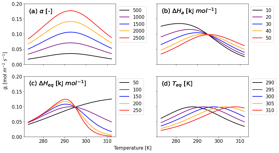
Figure 1 Calculated g_i as a function of canopy temperature for parameters (a) α, (b) ΔH_a, (c) ΔH_eq, and (d) T_eq from Eqs. (6) and (8). Each parameter is set to five different values given in the caption to investigate the response of g_i to temperature. While the target parameter changes, the other variables are fixed as α = 1400, ΔH_a = 40 kJ mol⁻¹, ΔH_eq = 100 kJ mol⁻¹, and T_eq = 295 K, which are initial values for Hyytiälä (see Sect. 2.3.2).

2.2 Observations

In optimizing the parameters g_s and g_i, we used the following variables obtained from observation to calculate COS leaf uptake (Eq. 1): the COS ecosystem flux, the COS soil flux, C_COS, temperature, and specific humidity, as well as GPP partitioned from NEE measurements. These data were collected and derived at Hyytiälä in Finland during 2013–2017 (Kooijmans et al., 2017; Sun et al., 2018; Vesala et al., 2022) and at Harvard Forest in the United States during 2012 and 2013 (Commane et al., 2015, 2016; Wehr et al., 2017). To validate the optimization results, we used the observation-based g_s and g_i (Sect. 2.2.2).

2.2.1 COS flux, GPP, and mixing ratio

We used canopy COS uptake derived from COS EC measurements for Hyytiälä (Kohonen et al., 2020; Vesala et al., 2022) and Harvard Forest (Wehr et al., 2017). The effect of storage in the canopy airspace was included by collocated COS profiles (Kooijmans et al., 2017; Kohonen et al., 2020).

GPP at Hyytiälä has been obtained from NEE using multi-year parameter fits (Kolari et al., 2014; Kohonen et al., 2022). For Harvard Forest, we chose to use the GPP derived from the isotope spectrometer measurements because it is more accurate and reliable with frequent and rigorous calibrations (Wehr et al., 2016).

COS soil flux measurements were available for the 2016 growing season at Hyytiälä and for the 2012 and 2013 growing seasons at Harvard Forest. For the soil flux in other years at Hyytiälä, we applied the monthly average diurnal cycle of the soil flux from 2016 to the other years (2013–2015 and 2017). The seasonal and diurnal variation of the soil flux is small compared to the total ecosystem uptake of COS (Sun et al., 2018). Hence, the averaged value of 2016 can be safely used for other years.

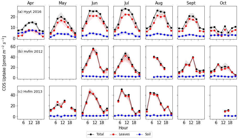
Figure 2 Monthly diurnal variation of COS fluxes in 2016 at Hyytiälä (a) and 2012–2013 at Harvard Forest (b, c). Lines are median values of each 3 h period, and the filled areas indicate the interquartile range (25 to 75 percentile). Black: COS ecosystem flux, blue: soil flux, red: vegetation flux estimated as ecosystem minus soil flux.

To convert the data frequency of observations to SiB4's 3 h time resolution, we calculated the median value of each variable in each 3 h interval and for each month. We only used data points when more than three data points were present and when all variables required for the optimization were available. Figure 2 shows the resulting average diurnal cycle per month for COS ecosystem, soil, and vegetation fluxes (ecosystem flux minus soil flux). Note that positive fluxes indicate uptake. Again, we note that we use the averaged soil flux at Hyytiälä because its variability is much smaller than the leaf flux.

2.2.2 Conductances g_s and g_i

Observation-based g_s was derived from sensible heat flux and evapotranspiration measurements using the flux gradient (FG) equations (Baldocchi et al., 1991; Wehr and Saleska, 2015, 2021). A key step in the derivation of g_s is the estimation of transpiration from evapotranspiration. At Harvard Forest, transpiration was estimated by an empirical equation established during times of minimal non-stomatal evaporation (i.e., a few days after rain, removing mornings with dew evaporation), as described in Wehr et al. (2017). At Hyytiälä, we simply restricted our analysis to periods of minimal non-stomatal evaporation by eliminating data when the dew point was equal to or greater than the air temperature or when the accumulated precipitation for the past 2 d was more than 0.01 mm.

The FG approach leads to significant uncertainties for nighttime data because the leaf-to-air water vapor gradient is too small under stable conditions (Wehr et al., 2017). We thus excluded nighttime g_s when the values were smaller than 0.05 mol m⁻² s⁻¹. To reduce the effect of random noise on g_s, we used an average diurnal cycle (based on 3 h medians) for each month.

Observation-based g_i was extracted by rewriting Eq. (1) as follows:

$$\begin{array}{}\text{(9)}& g_{\mathrm{i}}={\left({\displaystyle \frac{C_{\mathrm{COS}}}{F_{\mathrm{COS}}}}-{\displaystyle \frac{\mathrm{1.94}}{g_{\mathrm{s}}}}-{\displaystyle \frac{\mathrm{1.56}}{g_{\mathrm{b}}}}\right)}^{-\mathrm{1}}.\end{array}$$

Here, we used the observation-based g_s from the FG equation as discussed above and filtered observations of C_COS and F_COS. Additionally, we used simulated g_b from SiB4, as we do not have observed g_b available and as the value of g_b only has a minor effect on F_COS, which will be further discussed in Sect. 3.1. Although outliers of observed g_s, C_COS, and F_COS were removed already, a significant number of outliers in g_i appeared because of error propagation. To avoid excessive noise, we only retained g_i values in the interquartile range (25–75 percentile) of 3 h for each month.

2.3 Optimization

2.3.1 Procedure

In the optimization steps, we minimized a quadratic cost function J(x) based on Bayes' theorem (Tarantola and Vallette, 1982; Enting et al., 1993):

$$\begin{array}{}\text{(10)}& J\left(x\right)={\displaystyle \frac{{\left(x-x_{\mathrm{a}}\right)}^{\mathrm{2}}}{\mathrm{2}{\mathit{\sigma }}_{\mathrm{a}}^{\mathrm{2}}}}+{\displaystyle \frac{{\left(y-H\left(x\right)\right)}^{\mathrm{2}}}{\mathrm{2}{\mathit{\sigma }}_y^{\mathrm{2}}}}.\end{array}$$

Here, x represents the state, x_a the prior settings of the state, and σ_a the error assigned to the parameters. In the second term, y represents the observations and H(x) the model evaluation using the state x. The error σ_y represents the observational error. The details of σ_a and σ_y will be described in Sect. 2.3.2 and 2.3.3, respectively.

To optimize the g_s and g_i parameters, we intend to use the information from GPP and COS leaf uptake measurements sequentially. Thus, we propose a two-step approach in combination with an iterative minimization of the cost functions, as outlined in Fig. 3. In the first step, we optimally estimate g_s parameter b₁ by minimizing J(x) which sums GPP differences between estimation (H(b₁) in Eq. 10) and observation.

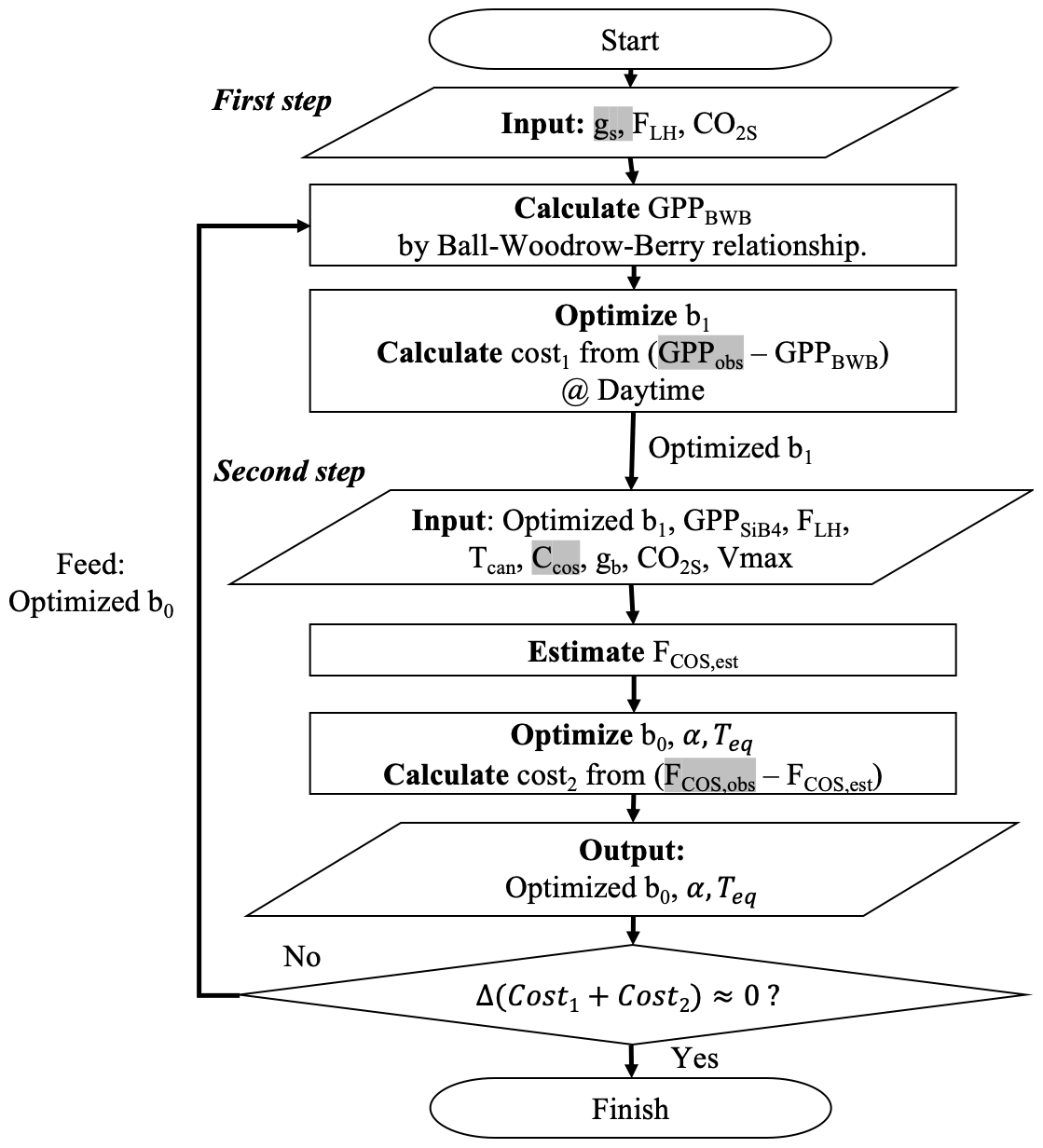
Figure 3 Flow chart of the procedure to optimize COS leaf uptake's parameters. The procedure has two steps: (1) optimize b₁ by minimizing deviations between GPP_BWB and observations; and (2) optimize b₀, α, and T_eq by minimizing deviations between modeled and observed COS uptake. Variables highlighted in gray are from observations, and the other variables are estimated from SiB4.

We select GPP for the first step optimization rather than g_s, because derived GPP from NEE has been evaluated more frequently than observation-based g_s. We use only positive GPP_obs values (uptake) because our target parameter b₁ in the first step cannot be optimized when GPP is zero. Here, we do not use GPP_SiB4 because SiB4 does not apply the BWB model for GPP calculation as described in Eqs. (3)–(5). For this reason, we cannot optimize BWB parameters with GPP_SiB4. Instead, we estimated GPP by rewriting the BWB model using an observation-based g_s (Sect. 2.2.2), modeled RH at the leaf surface (F_LH), and simulated CO_2s from SiB4. Hereinafter, the estimated GPP by the BWB model is called GPP_BWB:

$$\begin{array}{}\text{(11)}& {\mathrm{GPP}}_{\mathrm{BB}}={\displaystyle \frac{\left(g_{\mathrm{s}}-b_{\mathrm{0}}\cdot \mathrm{LAI}\cdot F_{\mathrm{RZ}}\right){\mathrm{CO}}_{\mathrm{2}\mathrm{s}}}{b_{\mathrm{1}}\cdot F_{\mathrm{LH}}}}.\end{array}$$

In the second optimization step, we optimize the b₀ and g_i parameters (α in Eq. 6 and T_eq in Eq. 8). These parameters are optimized by minimizing the differences between calculated and observed F_COS. F_COS is calculated with three conductances using Eq. (1). Specifically, g_s is estimated with Eq. (2) using the optimized b₁ from step 1. Here, we used GPP_SiB4 to satisfy our aim of optimizing the SiB4 model parameters. Note that GPP_BWB from Eq. (11) cannot be used here because it would make the estimated g_s equal to observation-based g_s. Based on sensitivity studies in Appendix A, we decided to select α, b₀, and T_eq as target parameters and to fix ΔH_eq and ΔH_a at 100 and 40 kJ mol⁻¹, respectively.

In the optimization procedure, we specifically exploit the fact that the nighttime COS flux carries information about nighttime g_s through the parameter b₀. The alternative, i.e., optimizing b₀ already in step 1, would ignore the information of nighttime g_s brought by COS flux observations. Consequently however, we have to iterate the procedure several times to reach convergence. Figure 3 specifies which observations and observation-based quantities are used in each step (g_s, GPP_obs, F_COS, obs, C_COS highlighted as grey) and which variables are simulated by SiB4 (e.g., T_can,F_LH, GPP_SiB4, CO_2s, g_b).

We applied the simplicial homology global optimization (SHGO) from the SciPy python library to minimize the cost functions. SHGO is appropriate for solving non-continuous, non-convex, and non-smooth functions (Endres et al., 2018). SHGO also allows the definition of a valid parameter range, as will be discussed in Sect. 2.3.2 and in Appendix A.

The V_max, rub was found to vary over the phenological stage and per PFT (Woodward et al., 1995; Wolf et al., 2006; Kattge et al., 2009; Walker et al., 2014), which also affects the calibration factor α. Therefore, we optimized α for each PFT and each phenological stage. In contrast, b₀, b₁, and T_eq were only separately determined for the different PFTs, assuming local characteristics for each PFT. We did not include V_max, rub in the state variables because this would require SiB4 CO₂ simulations. These simulations need several parameters, like carbon cycle pools, which are difficult to estimate. Therefore, we focus this research on estimating V_max, CA by optimizing g_i-related parameters.

2.3.2 Initial parameters and prior errors

The first term in the cost function (Eq. 10) ties the values of the parameters to realistic values. We additionally confined the parameter values within realistic physical ranges using the SHGO algorithm. Initial parameters and prior errors were chosen based on thresholds outlined in Appendix A, and they will be compared with optimized results in Sect. 3.3. The variation in the resulting cost function shows distinct differences between Hyytiälä and Harvard Forest, which reinforces our strategy to optimize parameters for each station separately.

2.3.3 Observation errors

To quantify the observational errors σ_y, we first calculated the 3 h average coefficient of variation (CV) relative to the mean of the observed COS vegetation flux in each phenological stage and observed GPP for the entire growing season. Figure 4 shows the results of observational errors. The GPP error is applied in step 1, and the COS leaf uptake error is used in step 2 in the optimization. We multiplied the CV with the mean in each phenological stage. Here, we classify the error of the COS leaf uptake in each phenological stage because we optimized α in each stage. In Fig. 4, we found that the errors differ slightly per phenological stage. At Hyytiälä, the errors are larger in the growth stage compared to the maturity stage, possibly due to the unstable weather conditions in growth stage. The COS leaf uptake error is larger at both stations during nighttime than during daytime. A potential reason can be the relatively higher uncertainty in the EC method during stable nighttime conditions.

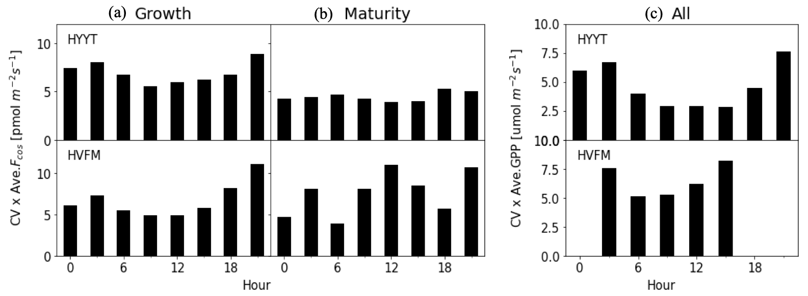
Figure 4 Distribution of the observation error in the growth (a) and maturity stages (b) for COS leaf uptake and all stages for GPP (c). The upper panel is the errors for Hyytiälä (HYYT) and the lower panel is for Harvard Forest (HVFM).

2.4 SiB4 simulations

We utilized several simulated variables from SiB4 in our optimization. Specifically, calculated GPP_SiB4, g_b, T_can, and V_max, rub and functions F_LH, F_RZ, and F_LC were used to calculate COS leaf uptake. In addition, LAI and CO_2s were used to estimate GPP_BWB. Furthermore, we introduced the new temperature function (f(T_can)_new) in the g_i calculation (Sect. 2.2.3) to calculate COS leaf uptake and excluded $P{P}_{\mathrm{sfc}}^{-\mathrm{1}}$ and $T_{\mathrm{can}}{T}_{\mathrm{0}}^{-\mathrm{1}}$ from Eq. (3) due to minor impacts of these factors for these ecosystems.

To simulate the vegetation assimilation F_COS at the two stations, we used the Modern-Era Retrospective Analysis for Research and Application, version 2 (MERRA-2) (Gelaro et al., 2017) as meteorological driver data. Only air temperature and leaf-specific humidity were taken from observations. To initialize the carbon pools, we spun up the model to equilibrate the pools. The spin-up was performed from 2000 to 2010 with 10 iterations. We used observed C_COS, and ambient CO₂ mole fractions were prescribed at 370 ppm.

To estimate the global impact of our findings, we performed a global SiB4 simulation from 2016 to 2018 to evaluate the influence of the new parameters on the monthly COS biosphere fluxes which are averaged for 3 years. The atmospheric COS mixing ratio C_COS were taken from optimizations using the TM5 chemical transport model (Ma et al., 2021; Kooijmans et al., 2021). We used 3 h C_COS averaged over 2016 to 2018 by Kooijmans et al. (2021). As we found that all target parameters differ between ENF and DBF (Appendix A), the application of the optimized parameters to other PFTs will likely be incorrect. Hence, we applied the optimized parameters only to ENF and DBF and used the standard values of SiB4 for the other PFTs. However, to confirm the f(T_can)_new effect on COS leaf uptake, we applied f(T_can)_new to all PFTs with averaged optimum T_eq from the two stations (303 K) and fixed ΔH_eq (100 kJ mol⁻¹) and ΔH_a (40 kJ mol⁻¹) as described in Appendix A. The soil flux is estimated following Ogée et al. (2016) as implemented by Kooijmans et al. (2021).

To examine the humidity stress impact in SiB4, we performed a simulation with and without the lower threshold for F_LH of 0.7 for ENF (see Sect. 2.1.2). Additionally, we replaced the RH at leaf level calculated by SiB4 by RH measured above the canopy. Results will be shown in Sect. 3.5.1. To account for the optimized humidity impact on the global COS leaf uptake, we simulated the global COS leaf uptake without the 0.7 threshold of F_LH for ENF.

2.5 Error reduction and statistics

To determine the uncertainty in the optimized model parameters, we employed a Monte Carlo optimization procedure as described in detail in Appendix B. In short, 100 optimizations were performed. In each optimization, we perturbed the state with random Gaussian noise on the state and the observations (Chevallier et al., 2007; Bosman and Krol, 2023), according to the errors in the state and observations (Fig. 4). Posterior error statistics will be reported in Table 3.

Additionally, we quantified the performance of the optimization by calculating the root mean square errors (RMSEs), mean bias errors (MBEs), and the chi-square metric (χ²). The χ² metric quantifies the average deviation from the observations, expressed in σ_y units. Thus, χ² = 1 signals that, on average, the model fits the observation within 1σ indicating a realistic error setting.

3 Results and discussion

3.1 Impact of each conductance

Figure 5 investigates which conductance contributes most to the total conductance (g_t). In these plots, all conductances are prior values before optimization. g_s and g_i were derived from observations (Sect. 2.2.2). We find that g_t is determined mainly by g_i and g_s. During daytime, g_i is the lowest conductance in almost all months at Hyytiälä but is comparable to g_s in Harvard Forest. The value of g_b is the highest and hence has the smallest impact on g_t. Therefore, to improve the accuracy of COS leaf uptake simulation effectively, parameters of g_s and g_i are evaluated and optimized, and g_b is kept to its standard value.

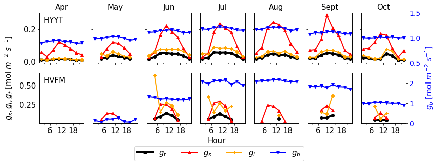
Figure 5 Monthly median value of diurnal conductances (black: g_t, red: g_s, orange: g_i, blue: g_b) at Hyytiälä (HYYT) and Harvard Forest (HVFM). g_b is estimated by SiB4, g_s and g_i are calculated based on observations as described in Sect. 2.2.2. Negative values are not displayed. The total conductance g_t is calculated from g_b, g_s, and g_i according to Eq. (1).

3.2 Optimization performance

We obtained optimized parameters after five iterations. By design, the optimized results reduced the deviations between model and observation of GPP and COS leaf uptake. This improvement is quantified by statistical indexes in Tables 1 and 2, respectively. GPP_BWB is improved slightly compared to the prior (Table 1), with RMSEs reduction from 4.08 to 3.84 µmol m⁻² s⁻¹ at Hyytiälä and 8.35 to 7.89 µmol m⁻² s⁻¹ at Harvard Forest. MBEs are decreased from −1.48 to −0.61 µmol m⁻² s⁻¹ at Hyytiälä and from −4.97 to −3.46 µmol m⁻² s⁻¹ at Harvard Forest (Table 1). The χ² was reduced by about 0.09 at Hyytiälä and by 0.08 at Harvard Forest. The improvement in GPP_BWB reflects the effect of optimizing b₁ and b₀ in the BWB model.

Table 1 RMSE, MBE, and χ² for the estimation of GPP_BWB in daytime using prior stomata parameters (pri) and posterior parameters (post).​​​​​​​

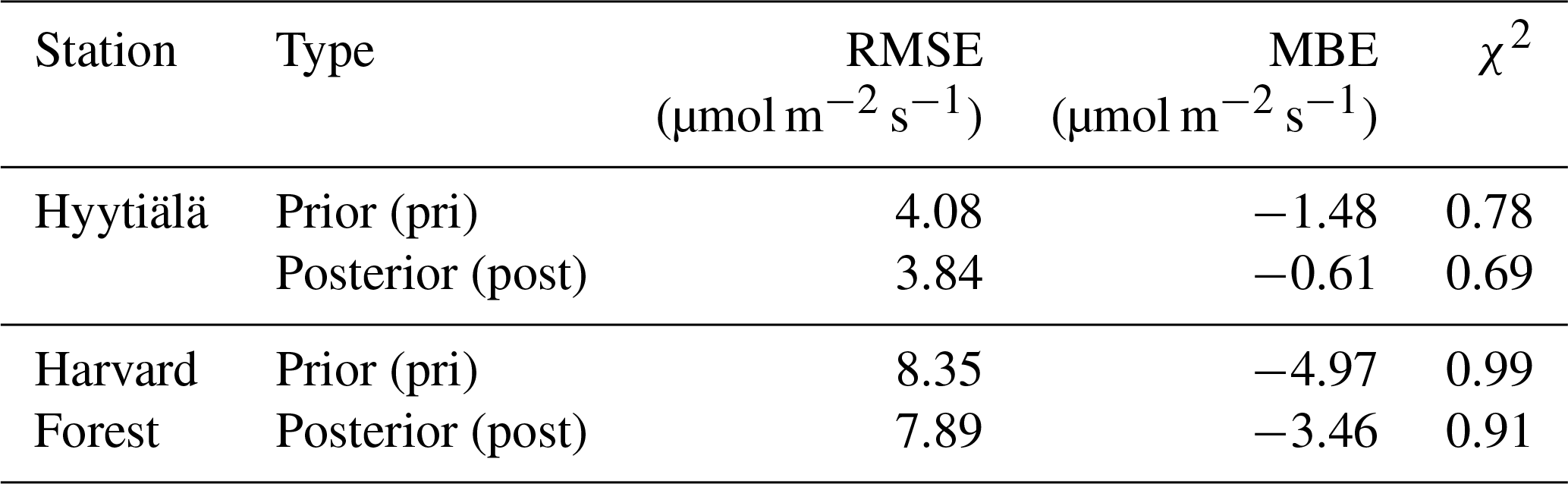
Table 2 Same as Table 1, but for COS leaf uptake, as applied in the original f(T_can)_SiB4 simulation with original conductance parameters (org), with the new temperature response function f(T_can)_new using the initial g_s and g_i parameters (pri), and with optimized parameters (post). Here, state parameters relevant for g_i are α and T_eq. The state parameters relevant for g_s are b₀ and b₁.

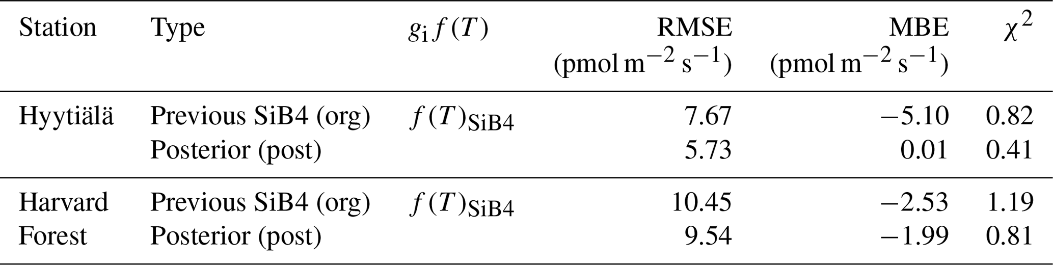
The posterior result of COS leaf uptake (“post” in Table 2) shows a slight improvement compared to the original-state variables with f(T_can)_new in RMSE (from 7.67 to 5.73 pmol m⁻² s⁻¹ at Hyytiälä and from 10.45 to 9.54 pmol m⁻² s⁻¹ at Harvard Forest) but significantly improved MBE (from −5.10 to −0.01 pmol m⁻² s⁻¹ at Hyytiälä and from −2.53 to −1.99 pmol m⁻² s⁻¹ at Harvard Forest, see “Post” in Table 2). The large RMSE reflects the typically large random noise of COS flux observations (Kooijmans et al., 2016; Kohonen et al., 2020). However, χ² drops by 0.41 at Hyytiälä and by 0.38 at Harvard Forest, confirming that the optimization properly reduced the mismatch between observations and the model within the error statistics. Figure 6 compares the optimized COS leaf uptake to the original SiB4 simulation in scatter plots. Where the original simulation with f(T_can)_SiB4 and previous-state variables was often underestimating the observations, the optimized results resemble the observations over a larger range of the data.

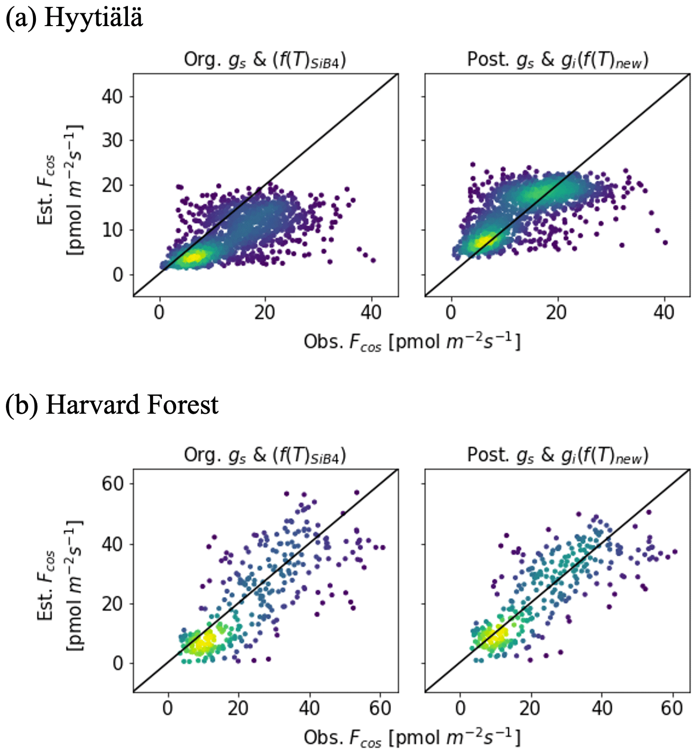
Figure 6 Scatter plots between observed and estimated COS leaf uptake from original parameters with f(T_can)_SiB4 (left) and optimized parameters with f(T_can)_new (right) for two stations. The colors represent the density of data.

3.3 Optimized parameters

The optimized parameter values with posterior errors are listed in Table 3. The optimized SiB4 parameters differ between the stations, likely because the dominant PFT and the climate conditions differ between Hyytiälä and Harvard Forest. For instance, the optimum temperature is smaller at Hyytiälä (19.85 K) than in Harvard Forest (35.85 K), which are slightly smaller than T_eq. Thus, the optimum temperature reflects the temperature dependence of the enzyme and its adaptation to temperature (Lee et al., 2007). This indicates that regional temperature information is important for correctly estimating g_i globally. The optimum temperature can be compared with other observations. For instance, Burnell and Hatch (1988) observed increasing CA activity with maize grown in a temperate temperature range from 20 to 30 ^∘C, relative to a temperature of 17 ^∘C. Thus, we can assume the optimal temperature lies above 17 ^∘C. Another study by Boyd et al. (2015) observed the C₄ plant Setaria viridis with a temperature of 28 ^∘C/18 ^∘C day/night, and a reduced CA activity is suggested at temperatures above 25 ^∘C. This optimum temperature falls between our values derived for Hyytiälä and Harvard Forest.

Table 3 Original (org) and optimized (post) state vectors for Hyytiälä and Harvard Forest in different phenological stages as defined by SiB4. Values of posterior in parentheses indicate posterior errors. The definition of the prior values is outlined in Appendix A, and the error reduction is described in Appendix B.

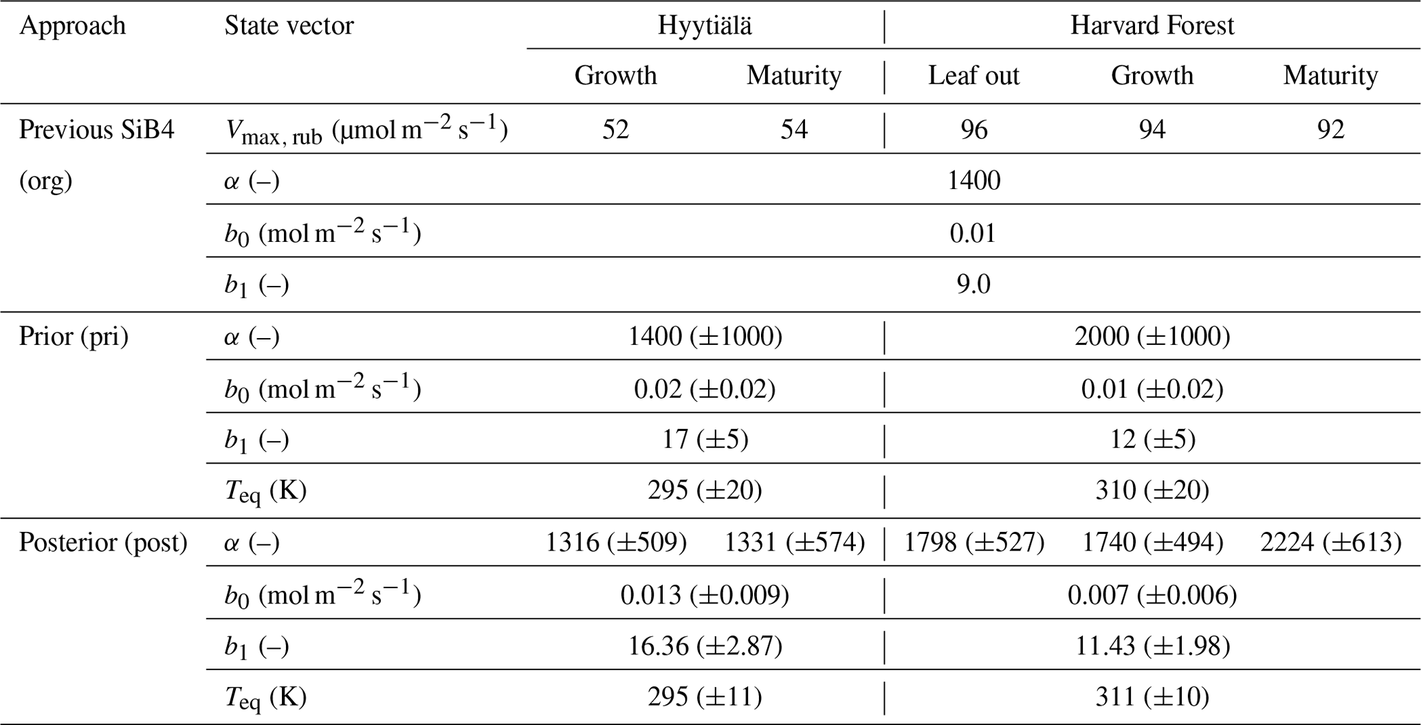
The α, which is the enzyme activity of CA relative to the V_max, rub, is reduced from the default value of 1400 to 1316 (in growth) and 1331 (in maturity) at Hyytiälä. At Harvard Forest, α values are larger than the original values in SiB4 for leaf-out (1780), growth (1740), and maturity (2224) phenological stages. Here it should be noted that the change of α should be interpreted in combination with the new temperature function f(T_can)_new of g_i. Since we only optimize T_eq for two PFTs (with identical and fixed values for ΔH_a and ΔH_eq) and T_eq only shifts f(T_can)_new (Fig. 1), the magnitude of g_i is primarily determined by parameter α. The different values of α derived for different phenological stages will be discussed in Sect. 3.4.

The optimized results of the BWB model parameters b₀ are similar to the original values used in SiB4, but b₁ values are mostly higher. The parameter values b₀ for Hyytiälä (0.013 mol m⁻² s⁻¹) and Harvard Forest (0.007 mol m⁻² s⁻¹) are slightly changed compared to the initial value (0.010 mol m⁻² s⁻¹). For the optimized BWB model parameter b₁, the empirical slope between g_s and GPP, we find a considerable increase at Hyytiälä (16.38) and a slight increase in Harvard Forest (11.43), compared to the prescribed SIB4 value of 9.0. Our optimized values are larger than the values presented in a review paper for the evergreen gymnosperm tree which showed b₁ = 6.8 and are similar to b₁ = 8.7 for the deciduous angiosperm tree (Miner et al., 2017). As will be discussed in Sect. 3.5, the higher slope at Hyytiälä is possibly related to an incomplete separation of observed transpiration rates from the latent heat flux.

Concerning the estimated errors in b₀, b₁, and T_eq, we find that errors have been reduced significantly compared to the prior error range. This indicates that the available data constrain these parameters well. Only the α parameters of Harvard Forest are less well constrained. Also, the skill of the optimization to independently optimize the parameters is high, as quantified by the posterior covariances that are presented in Appendix B.

3.4 Optimized temperature response

The optimized parameters show significant improvement in temperature response of the COS leaf uptake. Figure 7 presents the temperature dependency of g_i and COS leaf uptake from the original and optimized simulations output and observations. As stated before, the original f(T_can)_SiB4 describes the CA enzyme activity as an exponentially increasing response to temperature, which does not resemble the observations. The optimized g_i and COS leaf uptake follow the temperature dependence of the observation more closely than the original f(T_can)_SiB4. In Harvard Forest, an underestimated bias is shown at a lower temperature under 10 ^∘C, mostly corresponding to nighttime. This underestimate is related to the uncertainty in nighttime g_S and the small data volume at low temperatures (details in Sect. 2.2.2).

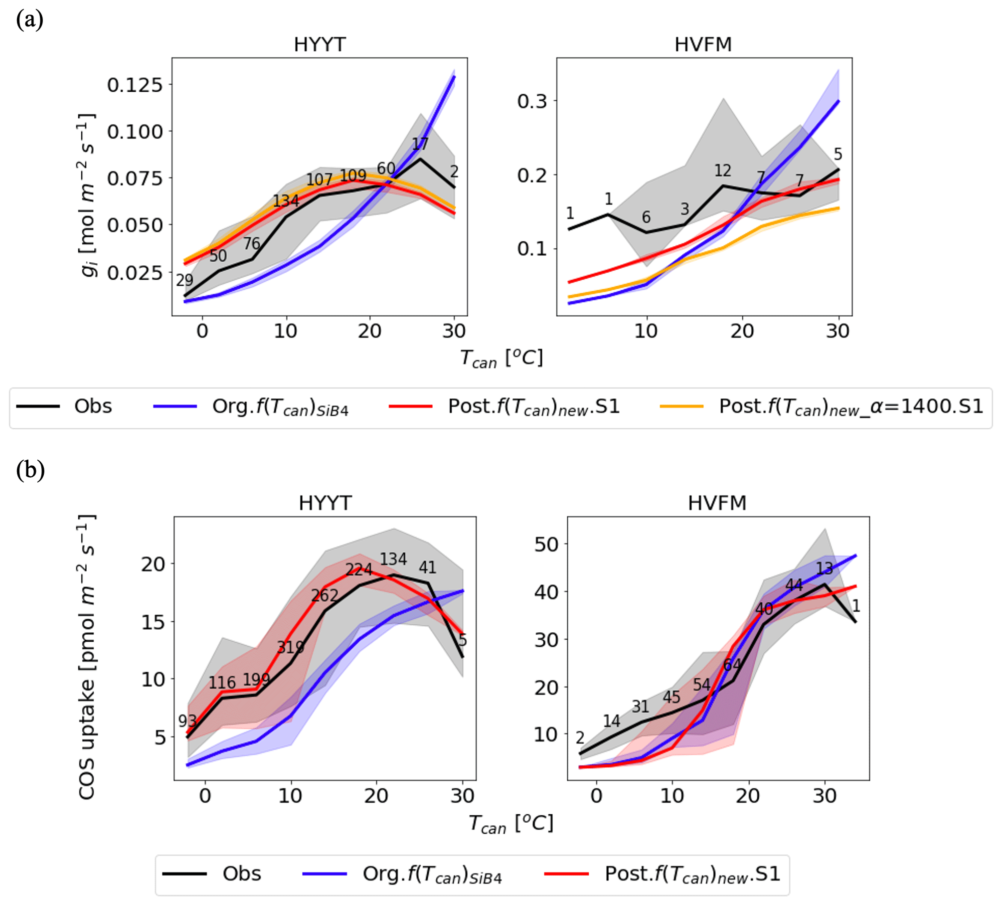
Figure 7 Temperature dependency on g_i (a) and COS leaf uptake (b) at Hyytiälä (HYYT; left) and Harvard Forest (HVFM; right). The lines are medians, and the filled area represents the 25 to 75 percentiles of each temperature range with 3 ^∘C intervals. Black: data based on observations; blue: previous parameters with f(T_can)_SiB4; red: optimized parameters with f(T_can)_new and g_s parameters of the BWB model; and orange: same as the red line, but now α is prescribed with original value (1400) and not optimized. The numbers indicate number of observations in each temperature bin.

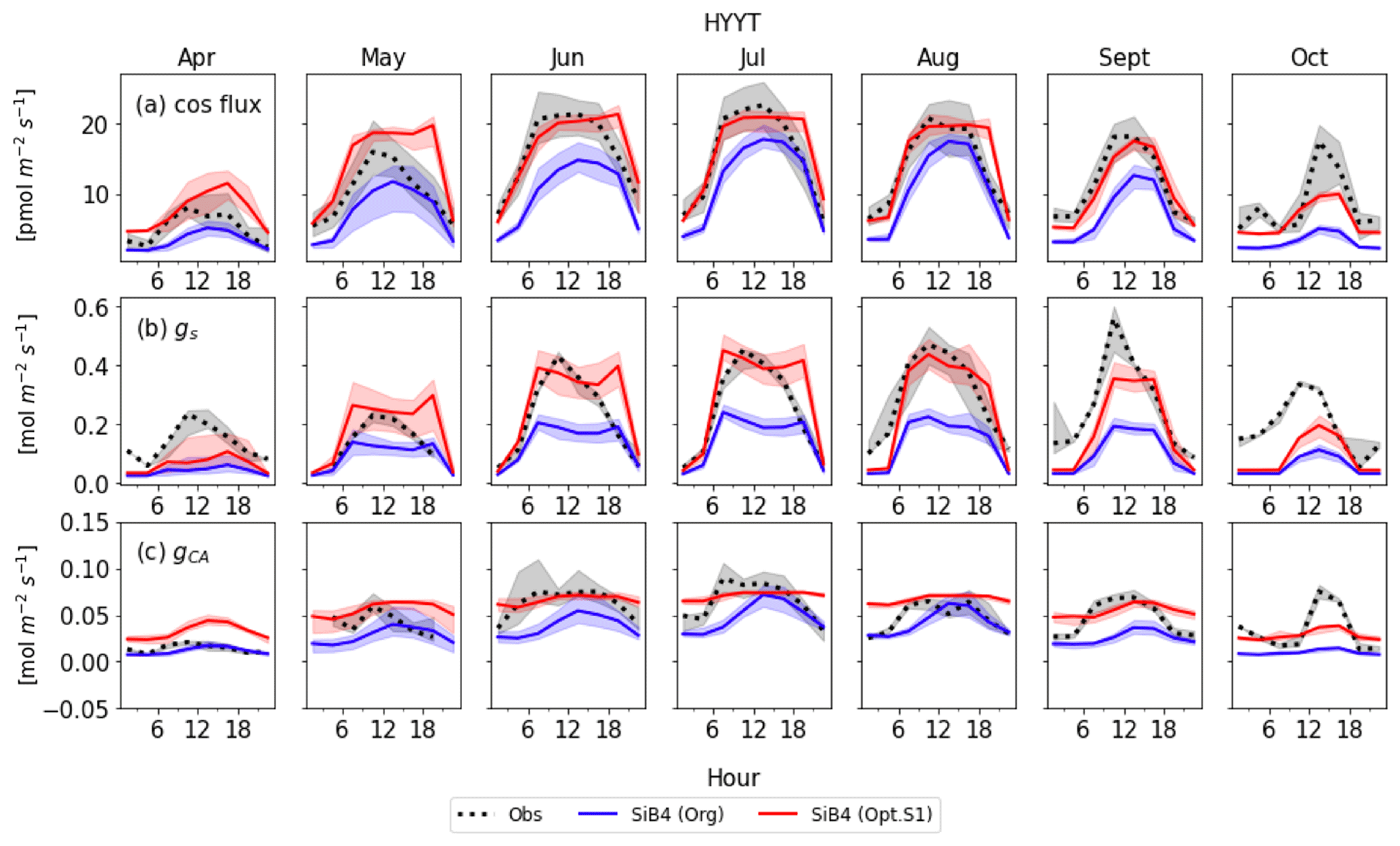
Figure 8 Monthly diurnal cycle of COS leaf uptake (a), g_s (b), and g_i (c) at Hyytiälä (HYYT) from 2012 to 2016. Data include observations (black dots), the original SiB4 model with f(T_can)_SiB4 (solid blue line), and SiB4 with optimized g_s and g_i parameters with f(T_can)_new (solid red line). The filled area corresponds to the 25–75 percentile of the data in each 3 h interval of each month.

In the upper panel of Fig. 7, we see the different roles of α and f(T_can)_new in the improvement of g_i response to temperature as the red and orange lines. Without the α correction applied (posterior with α = 1400; orange line), the optimized g_i resembles the fluctuations in the observations, but there remains a bias in the amplitude. In contrast, when the optimized value of α is included (red line), the amplitude of g_i is improved. Compared to the optimization that excluded α, the MBE is reduced from 0.006 to 0.003 mol m⁻² s⁻¹. Due to the different optimized α values in each phenological stage, the improvement of the red line shows the appropriate temperature responses. For instance, in Harvard Forest, α in leaf out and growth (1798 and 1740) mostly corresponds to lower temperatures. At these stages, the impact on g_i is smaller because g_i is smaller than that at high temperature. At high temperatures, there are more significant corrections of g_i, which correspond to the maturity stage value of α (2224).

The temperature responses of g_i and COS leaf uptake now show an optimum temperature. As can be observed in Fig. 7a, the optimum temperature of the observation-based g_i is seen as 293 K (19.85 ^∘C) at Hyytiälä. At Harvard Forest, the optimum temperature is 309 K (35.85 ^∘C) but falls outside the observation range. The optimum curve affects the COS leaf uptake at both stations with changing peak temperatures (Fig. 7b). The accuracies of g_i and F_COS are improved significantly at temperatures both below and above around the optimum temperature at both sites.

3.5 Application in SiB4

3.5.1 Monthly diurnal variation

Figures 8 and 9 display the SiB4 simulation results obtained with the original and optimized parameterizations compared to observations for Hyytiälä and Harvard Forest, respectively. As a result of the optimization, the monthly diurnal variation of the optimized COS vegetation flux, g_s, and g_i are closer to observations than the original SiB4 simulations. The observed COS leaf uptake and g_s show diurnal and seasonal fluctuations at both measurement sites, with the highest values around midday and in summer. For g_i, we observe a weak diurnal cycle throughout the year and higher daytime maximum values in summer, driven by the temperature dependence of CA.

Figure 9 Same as Fig. 8 but for Harvard Forest (HVFM).

At Hyytiälä, COS leaf uptake in the original SiB4 model was underestimated during daytime in all months. The fluxes increased too slowly in the morning for all months (Fig. 8a). These issues are solved by optimizing the BWB model parameters and temperature response function. In the case of g_s (Fig. 8b), the original SiB4 simulation showed the correct timing of the increase and decrease of g_s in the morning and afternoon but underestimated the peak daytime values. The optimized model now better resembles the daytime g_s values.

However, the model still overestimates g_s in the late afternoon of summer months at Hyytiälä. We speculate that one of the reasons lies in an inaccurate humidity, or humidity stress in SiB4. Figure 10 shows a diurnal cycle of g_s simulations averaged from April to August with different choices on how the humidity stress factor is treated (Sect. 2.5). When the default 0.7 threshold of humidity stress (F_LH) in ENF is applied in SiB4, g_s is overestimated in the afternoon at Hyytiälä (dotted blue line). When we removed the minimum threshold of F_LH for ENF, g_s simulations during midday are improved (note that the threshold was only implemented for ENF, not for DBF, and thus the blue dotted line is not visible for Harvard Forest in Fig. 10).

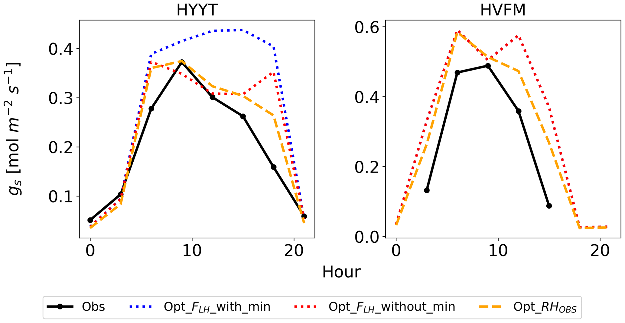
Figure 10 Average diurnal cycle of g_s at Hyytiälä (HYYT) and Harvard Forest (HVFM) from April to August. Data include observations (solid black line), SiB4 simulation with optimized parameters with minimum bounds of F_LH (dotted blue line) and without bounds (dotted red line), and with observed RH in air (dashed orange line). Note that the blue and red lines overlap for HVFM.

However, SiB4 still tends to overestimate g_s in the morning and late afternoon. The overestimated F_LH in SiB4 can result from three factors: (1) an overestimated water vapor flux in the boundary layer to the leaf surface, (2) an underestimated boundary conductance, or (3) an underestimated leaf surface temperature. Since we do not have observations of the leaf surface temperature, we have confirmed that the estimated canopy temperature has a tight 1 : 1 relationship with the observed air temperature. We speculate that the main reason for the overestimated F_LH is the uncertain water vapor flux. When we base the g_s calculation on the observed RH above the canopy, the diurnal cycle is better simulated (dashed orange line in Fig. 10). The overestimated water vapor pressure implies that SiB4 tends to underestimate the humidity stress in the late afternoon when converting observed specific humidity above the canopy to humidity at leaf surface level. We suggest evaluating the boundary conductance (point 2 above) with observations.

The optimized model still underestimates g_s at Hyytiälä in April, September, and October (Fig. 8b). This might indicate that we did not properly separate stomatal transpiration rates from the observed latent heat flux. The simulated mean ratios of evaporation to evapotranspiration in these 3 months are 66 %, 60 %, and 95 %, respectively, and these values are higher compared to the other months (43 % to 53 %). Thus, we speculate that the observed evapotranspiration does not solely represent stomatal transpiration in these months due to larger evaporation rates, leading to overestimated g_s in the observations.

Figure 8c shows that the optimized g_i often resembles the observed daytime g_i better than the original SiB4 simulation. Only in April is the optimized g_i overestimated at Hyytiälä. Again, this can likely be explained by the underestimated g_s, which is used to derive observation-based g_i (see Sect. 2.2.2).

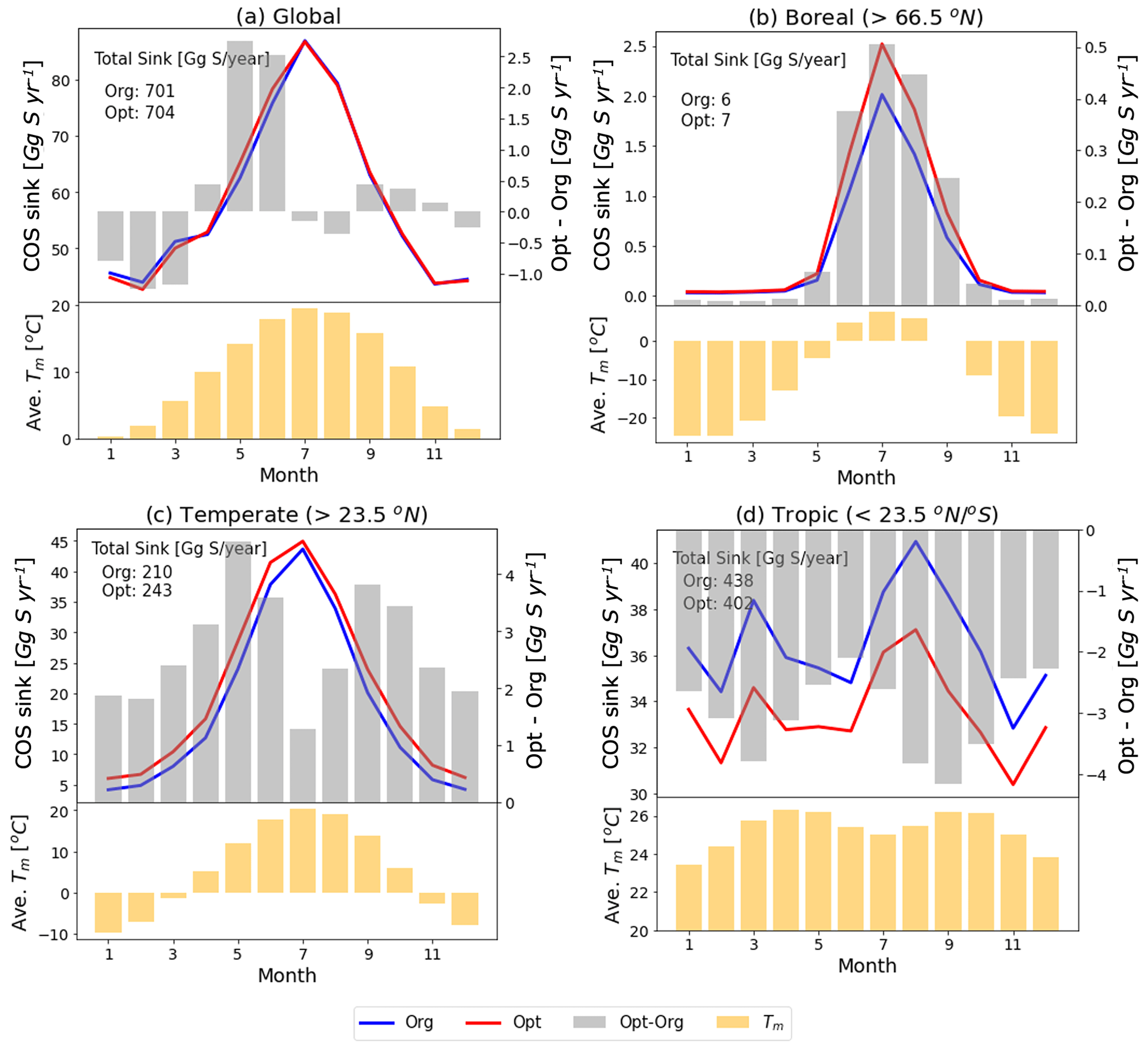
Figure 11 Monthly COS sink and averaged temperature in the mixed layer (T_m) over global (a) and specific regions (north boreal: b, north temperate: c, tropics: d) with the original (blue line) and the optimized (red line) SiB4 model. The grey bars represent the differences in COS sink between the original and the optimized model (right axis). The yellow bars are averaged temperatures in the mixed layer.

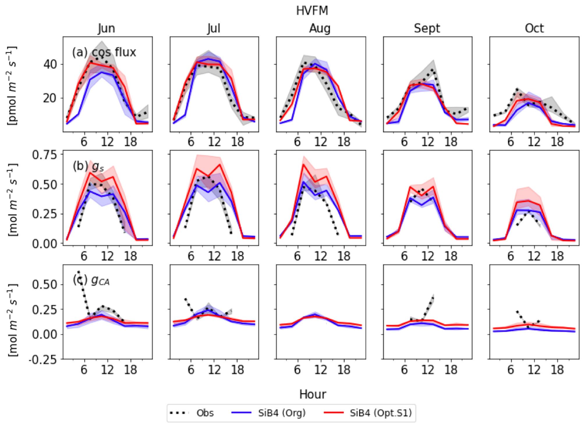
At Harvard Forest, the optimized SiB4 model generally simulates the magnitude of the COS leaf uptake well (Fig. 9a). The model overestimates the COS leaf flux only in the afternoon during the summer months. However, g_s values are generally overestimated, and SiB4 simulates two peaks during daytime. This indicates that humidity stress is only briefly occurring at midday in SiB4. However, in reality, the humidity stress likely remains a limiting factor in the afternoon under conditions with high vapor pressure deficit (VPD) (Kooijmans et al., 2019). Observations show that g_s typically peaks in the early morning and decreases in the afternoon due to higher afternoon VPD. Figure 10 shows that, similar to the Hyytiälä simulation, the afternoon decrease in g_s at Harvard Forest is better simulated when we use the RH observed above the canopy. In Fig. 9c, the optimized g_i during the daytime agrees well with the observation-based g_i, except for several drops or peaks in July and October, likely caused by observational errors or uncertainty of the observed g_s.

3.5.2 Global application

Figure 11 shows the SIB4 calculated changes in the monthly COS biosphere flux after applying the optimized temperature function and stomatal parameters. The global COS sink remains almost preserved (original: 701 Gg S yr⁻¹, optimized: 704 Gg S yr⁻¹), but the regional budgets change significantly. For example, the optimized model estimates larger COS uptake for all seasons in boreal and temperate regions and smaller uptake in the tropics. These changes are explained by the new temperature function of g_i in Fig. 7. However, since the new temperature function is based on only two observation sites in the boreal and temperate regions, the calculated uptakes need more verifications with observations obtained in other areas and in different climate conditions, such as the tropics.

The higher uptake at high latitudes and lower uptake at the tropics are nevertheless consistent with inverse modeling results presented in previous studies (Ma et al., 2021; Hu et al., 2021) and would help towards closing the COS budget. Still however, the temperature response function and BWB parameters are now based on measurements of only two sites in only two biomes. With more measurements over different vegetation types, these parameters could also be optimized for a wider range of ecosystems.

4 Conclusion

To simulate more accurate COS leaf uptake in the SiB4 model, we have proposed a new temperature function f(T_can)_new for the CA enzyme and have optimized g_s and g_i parameters using observations in ENF (Hyytiälä) and DBF (Harvard Forest) systems. The optimized model reduced the MBE from −5.10 to 0.01 pmol m⁻² s⁻¹ at Hyytiälä and from −2.53 to −1.99 pmol m⁻² s⁻¹ at Harvard Forest. Furthermore, χ² decreases by about 0.41 and 0.38, respectively.

The new function now considers an optimum temperature for enzyme activity, contrary to the initial temperature function used in SiB4 where an exponential increase of the temperature function was adopted from the RuBisCo enzyme activity. The new temperature function is characterized by an optimum temperature of 293 K (19.85 ^∘C) (Hyytiälä) and 309 K (35.85 ^∘C) (Harvard Forest). The new temperature response increases g_i, and thereby the COS flux when the temperature is below the optimum temperature (mostly at high latitudes), and decreases the COS uptake at higher temperatures. (e.g., close to the Equator). Globally, these modifications help to close gaps in COS budget that were identified in earlier studies. In this study, we have interpreted the decreasing g_i at higher temperatures as an optimum enzyme activity with the widely applied assumption that there are no COS emissions in leaves. However, COS emissions have recently been reported at high temperatures (Maseyk et al., 2014; Commane et al., 2016; Gimeno et al., 2017). To determine reasons for reducing COS leaf flux and internal conductance at high temperatures, it will be necessary to analyze the possibility that leaf emissions exist in observations in the future.

We have optimized the BWB model parameters for which we took advantage of the characteristics that the nighttime COS flux informs about nighttime g_s and thus the parameter b₀. The improved correspondence between model and observations shows that COS observations can help to constrain the relation between g_s and GPP better. In addition, we showed that SiB4 underestimates the leaf humidity stress under conditions where high VPD should limit g_s in the afternoon. This can be improved with more accurate relative humidity values and removing the threshold of humidity stress that was implemented in SiB4 specifically for ENF.

The optimized parameters show different values depending on the PFT. Therefore, extending our approach with more observations in different climate zones and over different PFTs will help obtain accurate COS fluxes on a global scale. This approach would reduce the uncertainty in the global COS budget and provide additional constraints on GPP.

Appendix A: State variable error settings

To evaluate the impact of the various parameters in f(T_can)_new in the optimization as state variables, we implemented a sensitivity test of a total cost function combined with cost₁ and cost₂, excluding the background term in the cost function equation (Eq. 10). Figure A1 shows the shape of the cost function when one parameter is varied within an acceptable range while the other parameters are fixed (Daniel et al., 2010; Sun et al., 2015) (details in Sect. 2.3.2). Based on the shape of the cost function, we used a pragmatic approach to select realistic parameter ranges. Variable values that push the cost function beyond 3.45 (Hyytiälä) and 5.14 (Harvard Forest) were considered outside the allowed physical range (red lines in Fig. A2). These thresholds are determined by the cost function value assuming that the modeled H(x) is the 75-percentile value of observation in 3 h observation in each month. Variables α, b₀, b₁, and T_eq (Fig. A1a, b, c, and f) have more significant impacts on the cost function than ΔH_a (Fig. A1d) and ΔH_eq (Fig. A1e). Overall, costs in Harvard Forest are higher than at Hyytiälä, likely because DBF has larger diurnal and seasonal variations in the observed fluxes than ENF. We set the optimization range as an initial value ±1.5 state error to apply SHGO algorithm.

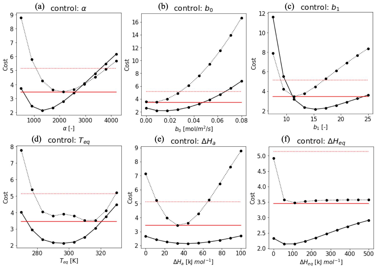
Figure A1 Cost function values plotted against the value of the state vector elements at Hyytiälä (solid line) and Harvard Forest (dotted line). The red lines indicate a criteria cost calculated by H(x) as the 75-percentile value of every 3 h observation in each month. While the target parameter changes, the other variables are fixed as α = 1400 (Hyytiälä), 2000 (Harvard Forest), ΔH_a = 40 kJ mol⁻¹, ΔH_eq = 100 kJ mol⁻¹, T_eq = 295 K (Hyytiälä), 310 K (Harvard Forest), b₀ = 0.02 (Hyytiälä), 0.01 (Harvard Forest), and b₁ = 17 (Hyytiälä), and 12 (Harvard Forest). These values were based on the value where the cost reached a minimum.

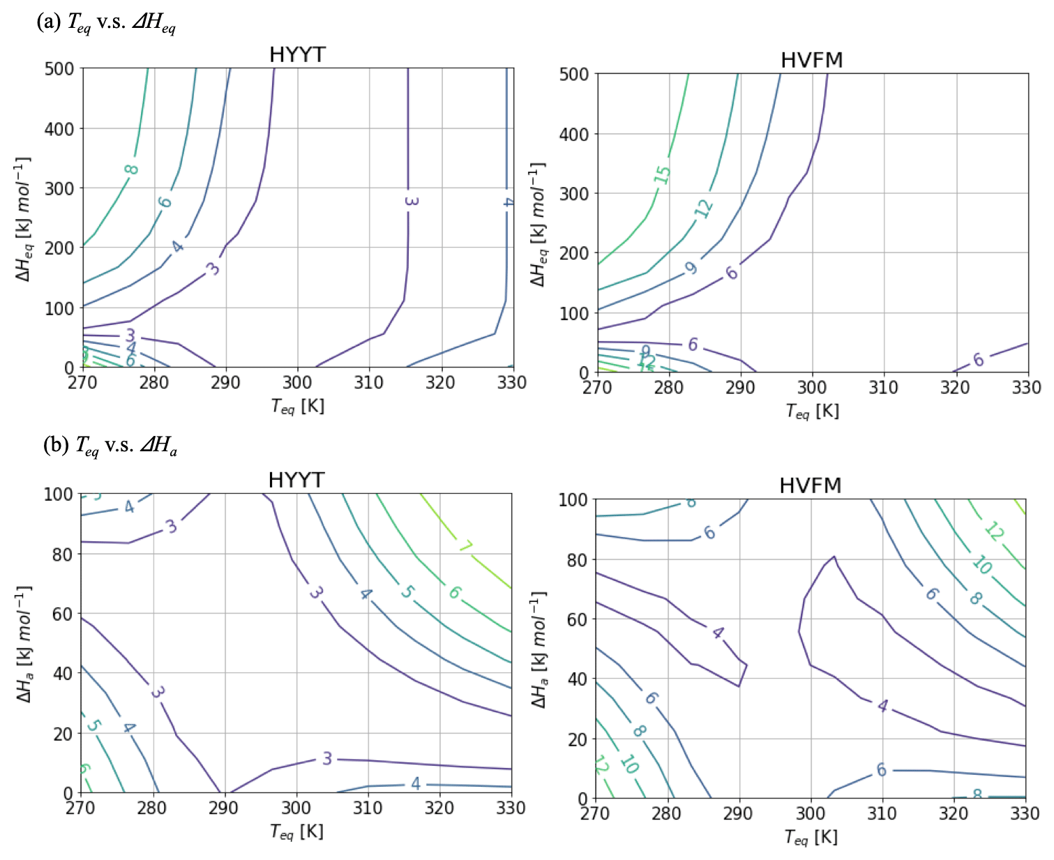
Figure A2 Contour diagram of the cost function value as a function of T_eq and (a) ΔH_eq and (b) ΔH_aat Hyytiälä (left) and Harvard Forest (right). While the target parameter changes, the other variables are fixed as Fig. A1.

Figure A2 shows contour diagrams of the cost function as a function of T_eq and other parameters of f(T_can)_new. The gradient is the cost function indicates the relative importance of each parameter. ΔH_eq does not interact with T_eq, but ΔH_a is inversely proportional to T_eq to minimize the cost. The cost function is most sensitive to variations in T_eq, and therefore we decided to fix ΔH_eq and ΔH_a at 100 and 40 kJ mol⁻¹, respectively, and to base our optimization on the state variables α, b₀, b₁, and T_eq.

Appendix B: Posterior uncertainties

To evaluate the ability of constrain the parameters, we performed an ensemble optimization with 100 different members. In each optimization, noise was added to the parameters (ε_a) and to the observation (ε_y). Random perturbations were drawn from a normal distribution with zero mean and standard deviations σ_a for the state parameters (x) and σ_y for the observations (y). The new cost function of an individual optimization thus becomes

$$\begin{array}{}\text{(B1)}& J\left(x\right)={\displaystyle \frac{{\left(x-x_{\mathrm{a}}+{\mathit{\epsilon }}_{\mathrm{a}}\right)}^{\mathrm{2}}}{\mathrm{2}{\mathit{\sigma }}_{\mathrm{a}}^{\mathrm{2}}}}+{\displaystyle \frac{{\left(y+{\mathit{\epsilon }}_y-H\left(x\right)\right)}^{\mathrm{2}}}{\mathrm{2}{\mathit{\sigma }}_y^{\mathrm{2}}}}.\end{array}$$

We optimized each ensemble with the same y (observationally derived GPP and COS leaf uptake) and x but added noise to each ensemble member (Chevallier et al., 2007). Subsequently, we calculated the posterior uncertainty as the 1 standard deviation of the posterior distribution of the optimized parameters.

Figure B1 shows the prior and posterior distribution of the parameters at the two stations. All posterior parameters show considerable reductions of variations (error), with optimized values that are listed in the main text in Table 3.

Additionally, we calculated a correlation matrix between the posterior-state parameters at the two stations, which is shown in Fig. B2. Overall, each parameter does not interact significantly (covariances < 0.7).

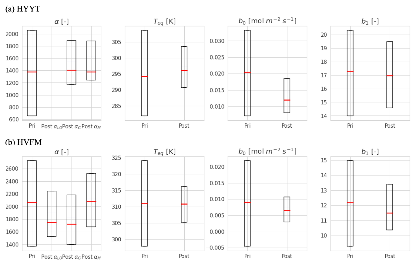
Figure B1 Error reduction of state variables in two stations (Hyytiälä (HYYT) and Harvard Forest (HVFM)). The red lines represent median values, and the boxes represent errors. Column “pri” shows the initial value and state error. Column “post” represents the mean of the optimized-state variables and the corresponding standard deviation. α_LO, α_G, and α_M indicate α in each phenological stage (leaf out, growth, and maturity, respectively).

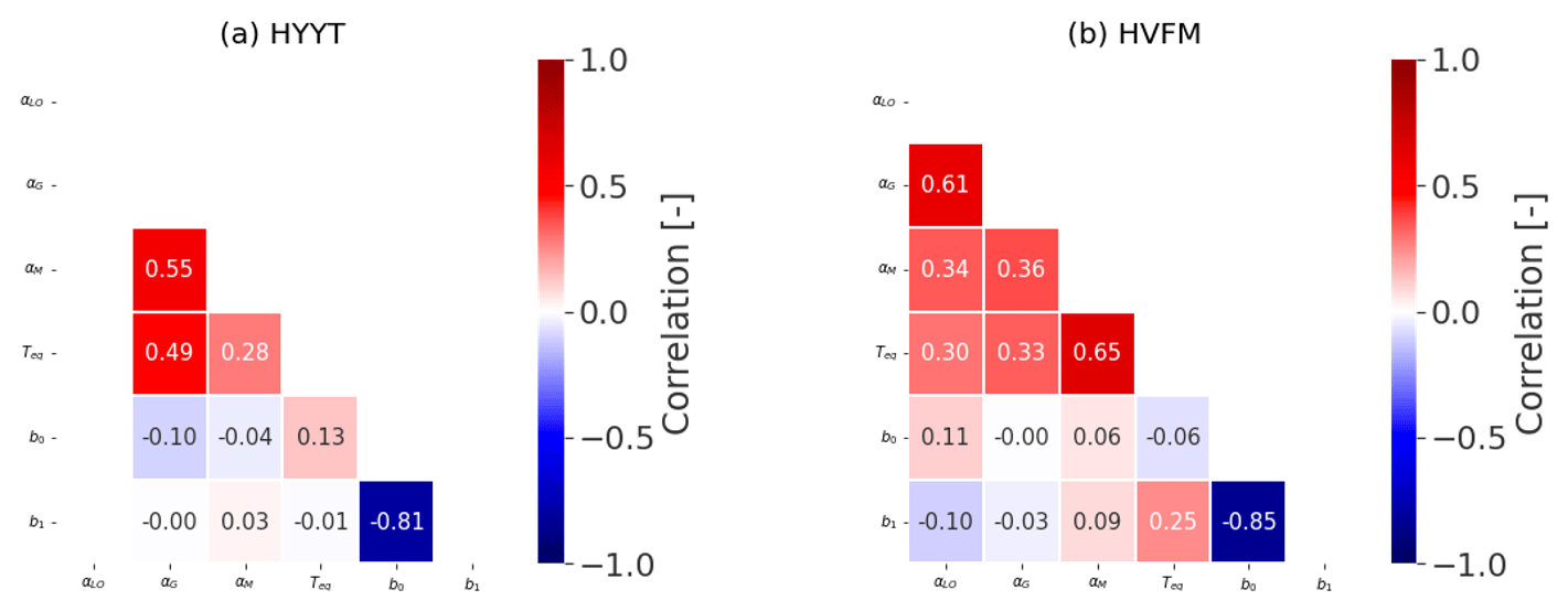
Figure B2 Covariance matrix for all state variables at Hyytiälä (HYYT) and Harvard Forest (HVFM).