the Creative Commons Attribution 4.0 License.
the Creative Commons Attribution 4.0 License.
 | 11 Aug 2023
Sub-frontal niches of plankton communities driven by transport and trophic interactions at ocean fronts
Inès Mangolte
Marina Lévy
Clément Haëck
Mark D. Ohman
Observations and theory have suggested that ocean fronts are ecological hotspots, associated with higher diversity and biomass across many trophic levels. The hypothesis that these hotspots are driven by frontal nutrient injections is seemingly supported by the frequent observation of opportunistic diatoms at fronts, but the behavior of the rest of the plankton community is largely unknown. Here we investigate the organization of planktonic communities across fronts by analyzing eight high-resolution transects in the California Current Ecosystem containing extensive data for 24 groups of bacteria, phytoplankton, and zooplankton. We find that a distinct frontal plankton community characterized by enhanced biomass of not only diatoms and copepods but many other groups of plankton such as chaetognaths, rhizarians, and appendicularians emerges over most fronts. Importantly, we find spatial variability at a finer scale (typically 1–5 km) than the width of the front itself (typically 10–30 km) with peaks of different plankton taxa at different locations across the width of a front. Our results suggest that multiple processes, including horizontal stirring and biotic interactions, are responsible for creating this fine-scale patchiness.
- Article
(16875 KB) - Full-text XML
- BibTeX
- EndNote


Ocean fronts are narrow regions of elevated physical gradients that separate water parcels with different properties (Hoskins, 1982; Pollard and Regier, 1992; Belkin and Helber, 2015). Some fronts are simply boundaries between biogeographical domains with distinct biological communities (Mousing et al., 2016; Tzortzis et al., 2021; Haberlin et al., 2019) that can overlap and mix in the frontal region (Lévy et al., 2014; Clayton et al., 2014). But many empirical and modeling studies have also pointed out that fronts can be specific “biological hotspots”, attractive to higher predators (Belkin, 2021; Prants, 2022) and often associated with an enhanced local productivity of diatoms (Allen et al., 2005; Ribalet et al., 2010; Taylor et al., 2012; Lévy et al., 2015). Theory has shown that frontogenesis, i.e., the intensification of a surface density gradient, leads to the vertical injection of nutrients into the euphotic zone (Klein and Lapeyre, 2009; Lévy et al., 2012; Mahadevan, 2016). Although this frontal supply of nutrients is generally assumed to propagate up the trophic web, the mechanistic link between nutrient supply and higher trophic levels is still very poorly understood, in large part because of the limited information on the intermediate trophic levels. Some studies have shown that the biomass and the activity of copepods are stimulated over fronts (Thibault et al., 1994; Ashjian et al., 2001; Ohman et al., 2012; Derisio et al., 2014) and that mesozooplankton acoustic backscatter (Powell and Ohman, 2015) and gelatinous zooplankton can aggregate at fronts (Graham et al., 2001; Luo et al., 2014). In addition, modeling studies suggest that the increased nutrient supply can create complex competitive interactions among phytoplankton groups over fronts (Lévy et al., 2014, 2015; Mangolte et al., 2022). Finally, fronts are associated with extremely dynamic horizontal currents that can transport water and their associated plankton communities over large distances (Clayton et al., 2013, 2017; de Verneil et al., 2019). In line with these different mechanisms, Lévy et al. (2018) proposed a rationalization of the biological impact of fronts, distinguishing between active (increased production in response to the nutrient injections), passive (stirring by horizontal currents), and reactive (biotic interactions) processes.
Here, we test the hypothesis that plankton communities at fronts are primarily shaped by the bottom-up transmission of the effect of the nutrient injections (“active processes”). To that end, we evaluate whether the taxonomic and spatial structures of the entire planktonic community (from bacteria to zooplankton) are consistent with a bottom-up response to nutrient injections. We then show that other processes, such as horizontal transport and trophic interactions (“passive” and “reactive” processes), also contribute to the structure of frontal communities, leading to plankton niches at a sub-frontal scale. More specifically, we address the following questions:
-
Are fronts commonly associated with a biological enhancement (“peak fronts”) or are they simply a boundary between two biologically distinct environments (“transition fronts”)?
-
In the case of peak fronts, are there changes in community structure associated with biomass enhancement? Do all species benefit from the frontal dynamics or are there winners and losers?
-
What is the spatial organization of the plankton community across a front? Is there biological variability at a scale finer than the physical scale across the front?
To answer these questions, we performed a meta-analysis of in situ data collected as part of the CCE-LTER (California Current Ecosystem Long-Term Ecological Research; Ohman et al., 2013) program during four cruises between 2008 and 2017 (Fig. 1 and Table 1). The CCE is an eastern boundary upwelling system with a strong regional cross-shore gradient from colder waters inshore to warmer waters offshore. This regional gradient is constantly stirred by the mesoscale horizontal circulation, which results in a multitude of small-scale density fronts (Mauzole et al., 2020). The CCE region is populated both by mesoscale eddies (Chelton et al., 2011), usually propagating westward, detectable from their sea surface height (SSH) anomaly and associated with geostrophic currents, and by coastal filaments originating from the coast and containing recently upwelled water parcels moving offshore through a combination of geostrophy and Ekman transport (Chabert et al., 2021). These two types of structures interact and lead to a complex interleaving of water masses separated by different types of frontal features forced by different processes (Renault et al., 2021; Mauzole et al., 2020).
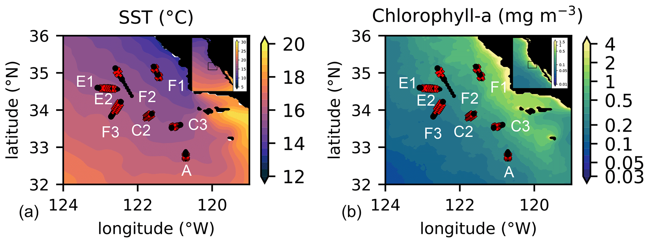
Figure 1Location of the transects sampled by the CCE-LTER program in summer and autumn between 2008 and 2017. Transect names (A, C2, C3, E1, E2, F1, F2, F3) are indicated close to the first station of their corresponding transect (note that the stations of E1 and E2 are in the same location, with E1 starting on the west and E2 on the east); stations identified as frontal stations are indicated by red crosses and stations identified as background stations by black circles. Transects E2 and F1 each contain 2 fronts, leading to a total of 10 fronts for the 8 transects. Background color: July climatology over the study period (2008–2017) of (a) SST and (b) chlorophyll a.
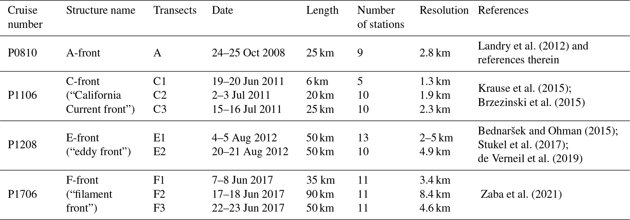
Table 1Name and characteristics of the eight CCE-LTER transects. C1 was aborted and is not included in this study.
The empirical measurements include the quantification of the biomass of 24 taxa in the planktonic community, from heterotrophic and cyanobacteria to phytoplankton and mesozooplankton (Fig. 3). The data were collected along eight high-resolution transects (with a spacing of 1 to 5 km between stations) conducted across various structures, including upwelling filaments and geostrophic fronts; we identified 10 separate fronts from gradients in thermodynamical properties (density, temperature, salinity), as two transects crossed filaments with fronts on either side.
We first investigate whether the various groups of plankton have enhanced biomass over fronts compared to the fronts' immediate surroundings (the “background”). We find that over most fronts, there is a specific frontal plankton community characterized by biomass maxima of diatoms and many zooplankton taxa as well as minima of other phytoplankton taxa, particularly cyanobacteria. Then, we examine the fine-scale spatial organization of the planktonic community by describing the width and the position along the transect of these biomass peaks relative to the width of the density gradient. We find that, contrary to expectations from the theoretical structure of vertical circulation at fronts (Klein and Lapeyre, 2009), the biomass peaks are not aligned with the density gradient, and their locations show an unexpectedly high level of variability among taxa. Finally, in the Discussion section, we evaluate the implications of these observations in terms of the driving processes, paying attention to their consistency with the hypothesis of a purely bottom-up system reacting to a frontal supply of nutrients.
We used data collected during four cruises of the CCE-LTER program (Table 1). During each cruise, one to three transects were conducted across frontal structures (Fig. 1). Physical, chemical and biological properties were measured at 9 to 12 stations regularly spaced at high resolution (1–5 km between stations) along the transects and were all performed in a single night (Fig. 2). At each station, 24 different plankton taxa were identified using measurements made using a CTD rosette for bacteria and phytoplankton and a net tow for zooplankton (Fig. 3). Other measurements included Chl-a fluorescence and the concentration of macronutrients. Importantly, the same observations and methodology were applied for all CCE-LTER transect cruises, which provides a consistent dataset, although the data were collected in different years. Our method relies on the comparison between the plankton community over the fronts and the community in the waters immediately surrounding the fronts. We also examine the fine-scale organization of the plankton community across the front. The first step in our analysis is thus the identification of the stations that we identify as frontal stations, and we compare the community structure at these stations with the community structure in the neighboring background stations.
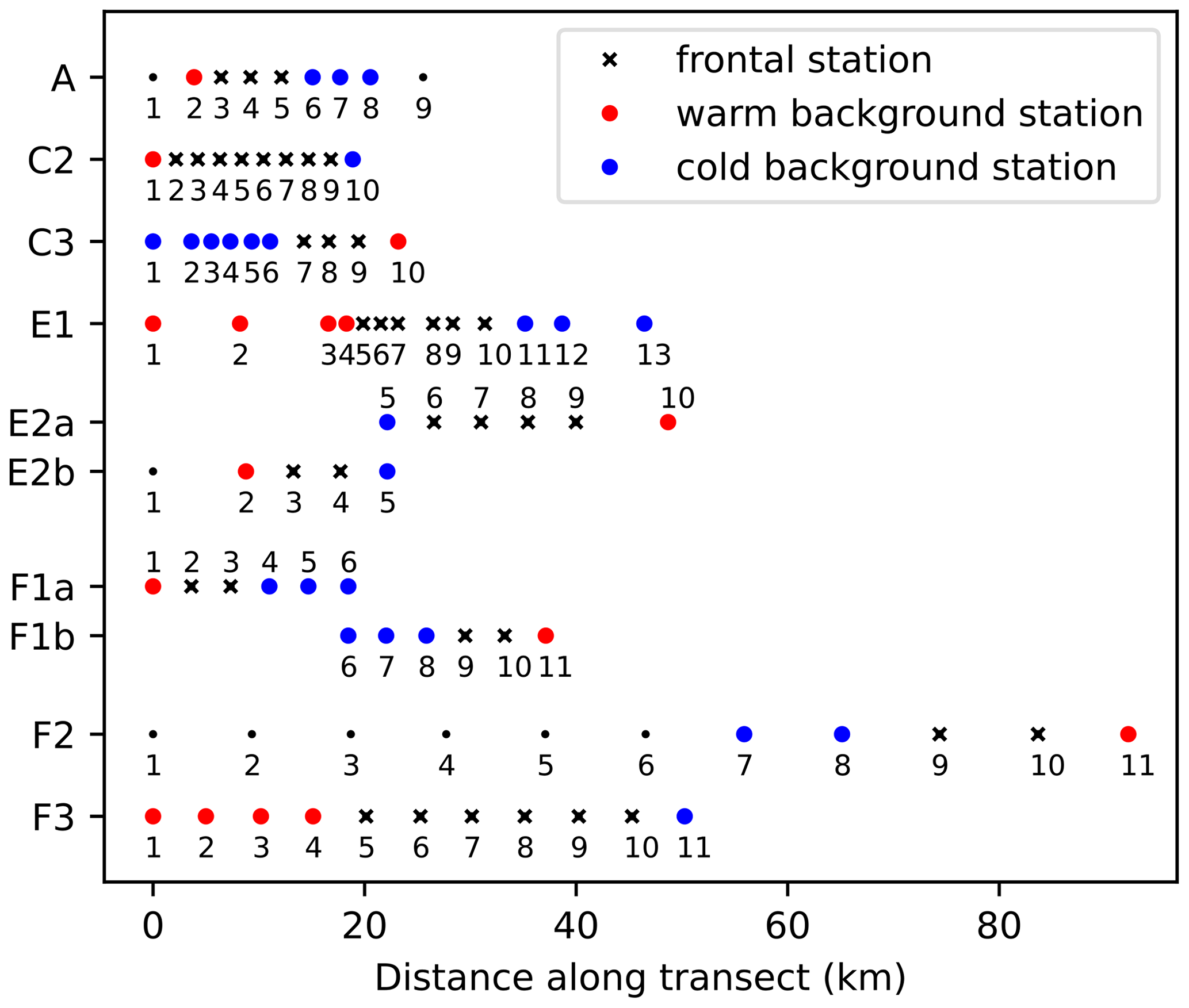
Figure 2Number of stations and spacing between stations along each of the eight CCE-LTER transects. Stations are classified into frontal stations (black crosses) and background stations on the warm side of the front (red dots) or cold side of the front (blue dots); small black dots indicate stations that were excluded from the analysis (see text). Note that transects E2 and F1 contain two fronts and are shown twice (E2a/E2b, F1a/F1b), once for each front, with empty circles over the second front.
2.1 Data
At each station, a CTD vertical profile was conducted down to 100 m, and water samples were collected in Niskin bottles at discrete depths on the ascent; zooplankton samples were then collected with a 202 µm mesh vertical Bongo net tow (also from 0 to 100 m). In addition to the temperature and salinity recorded by the CTD, a fluorometer measured the in vivo chlorophyll-a fluorescence along each vertical profile (California Current Ecosystem LTER and Goericke, 2017). The concentration of macronutrients (nitrate, phosphate, silicic acid, nitrite, and ammonium) was determined at discrete depths from the Niskin bottle samples (California Current Ecosystem LTER and Goericke, 2022). The plankton samples were later analyzed on land using three different methods (Fig. 3):
-
Flow cytometry was performed on the Niskin bottle water samples (0–100 m), producing the abundance (number of cells L−1) of four taxa of picoplankton (<2 µm) identified by their light-scattering properties: Prochlorococcus (PRO), Synechococcus (SYN), heterotrophic bacteria, and picoeukaryotes (California Current Ecosystem LTER and Landry, 2019a).
-
HPLC (high-performance liquid chromatography) was performed on all the Niskin bottle samples (0–100 m) during the first cruise (A-front) and on the surface Niskin bottle only for the other three cruises (E-front, C-front and F-front). The concentrations of chlorophyll a and accessory pigments were measured and used to determine the contributions (percentage) of eight phytoplankton taxa relative to the total chlorophyll (Goericke and Montoya, 1998; California Current Ecosystem LTER and Goericke, 2019).
-
Zooplankton samples were collected using vertical Bongo nets (0.71 m diameter, mesh size 202 µm) retrieved from 100 m, preserved in 1.8 % buffered formaldehyde, and the organisms then identified in the lab using the ZooScan semi-automated imaging system (Gorsky et al., 2010; Ohman et al., 2012) with 100 % manual validation. The analysis produced the vertically integrated abundance (number of organisms m−2) of 15 groups of mesozooplankton. The abundances of eggs (mainly belonging to copepods and euphausiids) and nauplii (the juvenile form of copepods and other crustaceans) were also determined; the ratio of eggs or nauplii to adults is used as a proxy of secondary production (Mangolte, 2023a).
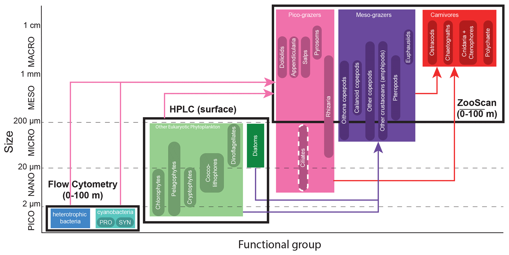
Figure 3The 24 plankton taxa measured as part of the CCE-LTER program, sorted by size class (y axis) and trophic group (color). Shown are the different instruments used to measure their abundance (black rectangles). Arrows represent the main predatory interactions between groups: picograzers consume bacteria and phytoplankton, mesograzers consume eukaryotic phytoplankton, and carnivores consume grazers. Flow cytometry produces the abundance of heterotrophic and cyanobacteria collected in Niskin bottles at discrete depths (about even levels from 0–100 m). HPLC produces the concentration of six taxa of eukaryotic phytoplankton collected in Niskin bottles at discrete depths for the A-front and at the surface only for the other cruises. ZooScan produces the vertically integrated abundance (0–100 m) of 15 taxa of zooplankton collected with a Bongo net tow. Flow cytometry includes two types of cyanobacteria: Prochlorococcus (PRO) and Synechococcus (SYN). Nano- and microzooplankton (such as ciliates) were only sampled in the A-front cruise (using epifluorescence microscopy) and are not part of this meta-analysis.
The 24 individual taxa were then grouped into seven functional groups. The functional groups were defined on the basis of their ecological and biogeochemical roles rather than size and taxonomy. For instance, diatoms were separated from the other eukaryotic phytoplankton because of their high potential for growth under nutrient-replete conditions, while rhizarians and tunicates were included in the picograzers group because they all consume bacteria despite the former being protists and the latter metazoans. Since the different instruments provide measurements in different units, the abundances of the taxa were first converted into carbon biomass, which served as the common currency, and then they were summed to obtain the total for each group. Appropriate conversion factors were chosen according to the literature and include carbon content per cell for flow cytometry (Garrison et al., 2000), chlorophyll : carbon ratios for HPLC (Li et al., 2010), and carbon per organism values for ZooScan (Lavaniegos and Ohman, 2007). The vertically resolved data derived from Niskin bottles (flow cytometry for all the transects and HPLC for the A-front) were then vertically averaged. Thus all the data are expressed as a carbon concentration (µgC m−3).
It should be noted that nano- and microzooplankton (which mainly consist of heterotrophic protists such as nanoflagellates and ciliates) were also measured during the A-front cruise using epifluorescence microscopy (Taylor et al., 2012; California Current Ecosystem LTER and Landry, 2019b). However, they were not sampled during the subsequent cruises and thus are not included in this meta-analysis. Cyanobacteria (PRO and SYN) were measured by both flow cytometry and HPLC; flow cytometry data were depth-resolved in all transects, while the HPLC data were only depth-resolved in the A-front transect (the other transects only include the surface value). There are some quantitative differences between the data produced by the two methods, but the patterns are generally similar (Figs. A6 and A7 in the Appendix). In the following analysis, we use the flow cytometry data since they are vertically resolved. Finally, picoeukaryotes (measured with flow cytometry) were not incorporated in our analysis because they include photosynthetic and heterotrophic organisms that belong to different functional groups. The photosynthetic picoeukaryotes were, however, measured independently by HPLC. Moreover, because the category includes a vast variety of organisms with a wide range of carbon content values, they could not be robustly converted to carbon biomass.
2.2 Identification of fronts
During the CCE-LTER cruises, fronts were first roughly identified using real-time satellite data of sea surface temperature (SST) and SSH and their location and physical structure more precisely localized with the free-fall Moving Vessel Profiler (MVP; Ohman et al., 2012). This permitted the transects to be successfully positioned in the cross-frontal direction. All transects show distinct density and/or temperature and salinity gradients, indicating the presence of a front (uppermost panels in Fig. 4). Each front is sampled by at least one station and in most cases at least three. Two of the transects (E2 and F1) crossed a cold filament and thus included two fronts, each corresponding to one boundary of the filament. These two transects were separated in two half-transects prior to analysis at the center of the filament (station 5 in transect E2 and station 6 in transect F1, indicated by vertical lines in Fig. 4). This led to a total of 10 segments, each containing one front (Fig. 2). In this section, we describe the common procedure we applied to identify these 10 fronts; their individual characteristics and their temporal evolution (up to a few months before and after each transect, reconstructed with satellite data as described in Sect. 2.5) are presented in detail in the Appendix.
Along each segment, we sorted the stations into those belonging to fronts (black crosses in Figs. 2 and 4) and those in the background, separating the cold side and warm side of the front (blue and red circles in Fig. 2, respectively). This was done on the basis of the along-transect gradients of density, temperature, and salinity, averaged between the surface and 50 m. Gradients were computed using central differences except at the boundaries where one-side differences were used. The distributions of density, temperature, and salinity and their gradients along the transects showed a variety of situations: the sign and intensity of the density gradients strongly varied among transects, as well as their structure (Figs. 4 and A9). Some fronts were clearly associated with marked density gradients (A, E1). Another (C2) was compensated (i.e., there was no significant density gradient, but there were marked temperature and salinity gradients), while others consisted of density steps (e.g., F3).
To sort the stations, we used the absolute values of the gradients and normalized them by their averaged value along the transect (hereafter Δρ, ΔT and ΔS are the normalized gradients, and they are equal to 1 when the gradient is equal to the mean gradient). In order to capture the variety of situations described above, we used the following criteria to identify frontal stations and background stations:
-
Stations where Δρ>1 or ΔT>1 or ΔS>1 were classified as a front, unless they were at the edge of a transect.
-
Some stations have relative gradients lower than 1 but are located between frontal stations; these stations constitute steps of a larger frontal structure and are also classified as frontal stations. This was the case for stations 5–6 of transect C2 and station 8 of transect F3.
-
Isolated stations with strong gradients outside of the targeted frontal area were excluded from the analysis (meaning they are neither front nor background) when they were part of a separate physical structure. This was the case for station 9 of transect A and station 1 of E2b where density variations reflect the large-scale cross-shore gradient; for station 1 of transect A that is located at the edge of the California Current, with a salinity gradient of opposite sign from the main front; and for stations 1–6 of transect F2 that are part of another filament (see the Appendix text).
-
Stations where Δρ>1 or ΔT>1 or ΔS>1 located at the edge of a transect were classified as background in order to provide at least one point of comparison with the other frontal stations of the transect. This was the case for station 11 of transect F3, station 1 of half-transect F1a, station 5 of half-transect E2b, and station 1 of transect C2.
-
All remaining stations were classified as background.
Within background stations, we then identified those located on the cold (or warm) side of each front. Finally, we identified the central position of the front (in km) and the width of the front, defined as the number of front stations multiplied by the resolution of the transect (in km).
2.3 Front enhancement factor
We quantified the biological effect of each front by measuring a front enhancement factor (FEF) for each plankton taxon, as well as for total phytoplankton biomass and Chl-a fluorescence. The FEF was computed when there was a biomass peak at the front and was undefined otherwise. A peak at the front implied that the taxon has an extremum in biomass (maximum or minimum) at one of the frontal stations, relative to values on both sides of the front. We defined the FEF as the relative difference between the peak biomass at the front and the average biomass in the background stations surrounding the front:
where Fpeak is the biomass extremum among frontal stations (minimum or maximum), and is the average biomass of the background stations (including cold side and warm side).
2.4 Position and width of biomass peaks
Along each transect, taxa exhibited large changes in their biomass at the scale of a few stations, with clearly recognizable peaks (Figs. 4, A11, A12 and A13). To complement the FEF, which gives the intensity of the biomass peaks, we described the spatial structure of the biomass peaks by recording their position (center of the peak) and their width. It is important to note that the biomass peak detection and the location of the physical fronts are made independently of one another, the latter on the basis of the along-transect distribution of density, temperature, and salinity and the former on the basis of the along-transect distribution of the biomass of taxa. While most biomass peaks were located over frontal stations, some were outside of the fronts. We then compared the location of the biomass peaks with the location of the physical front by measuring the difference between their positions (in km), with the sign indicating whether the biomass peak is on the warm side of the front (positive values) or the cold side (negative values).
2.5 Temporal evolution of the fronts
The temporal evolution of the fronts in the weeks leading to and following the in situ transects was evaluated using satellite data. For SST, CHL, and SSH, we used datasets distributed by the Copernicus Marine Environment Monitoring Service (https://marine.copernicus.eu/, last access: 22 August 2022): the ESA CCI/C3S SST (https://doi.org/10.48670/moi-00169), the Globcolour Chlorophyll (https://doi.org/10.48670/moi-00281), which are both 4 km daily “cloud-free” products, and the GLORYS reanalysis SSH product (https://doi.org/10.48670/moi-00021) at 8 km resolution. To characterize frontal structures more accurately, we combined two complementary approaches: the first is based on the detection of strong gradients in the SST, which are quantified by a heterogeneity index (HI; methods of Liu and Levine, 2016; Haëck et al., 2023). The HI was computed daily at 4 km resolution, based on the ESA CCI/C3S product, but is limited by cloud cover. The second is based on the detection of stirring structures and regions of convergence, quantified by backward in time finite-size Lyapunov exponents (FSLEs; D'Ovidio et al., 2004; Fifani et al., 2021). The FSLEs were computed from horizontal velocities combining geostrophic currents derived from altimetry and Ekman currents derived from wind-stress data (Chabert et al., 2021), but its accuracy with fine-scale structures is limited by the low resolution of altimetry data. Finally, to evaluate the history of the water parcels, we used the water age, defined as the time elapsed since a parcel of water left the coast (defined as the 500 m isobath) and computed by advecting water parcels backwards until they reach the coast (Chabert et al., 2021).
Snapshots of these satellite-based products at the time of each transect are shown in Figs. A1, A2, A3, and A4, and videos of their evolution over 6 months are available as video supplements (Mangolte, 2023b, c, d, e).
In the next sections, we first describe the composition of the frontal community (i.e., the presence and intensity of biomass peaks at the front for the various plankton taxa using the enhancement factor) and secondly its spatial organization across the fronts (in terms of width of the peaks and position along the transect relative to the density gradient).
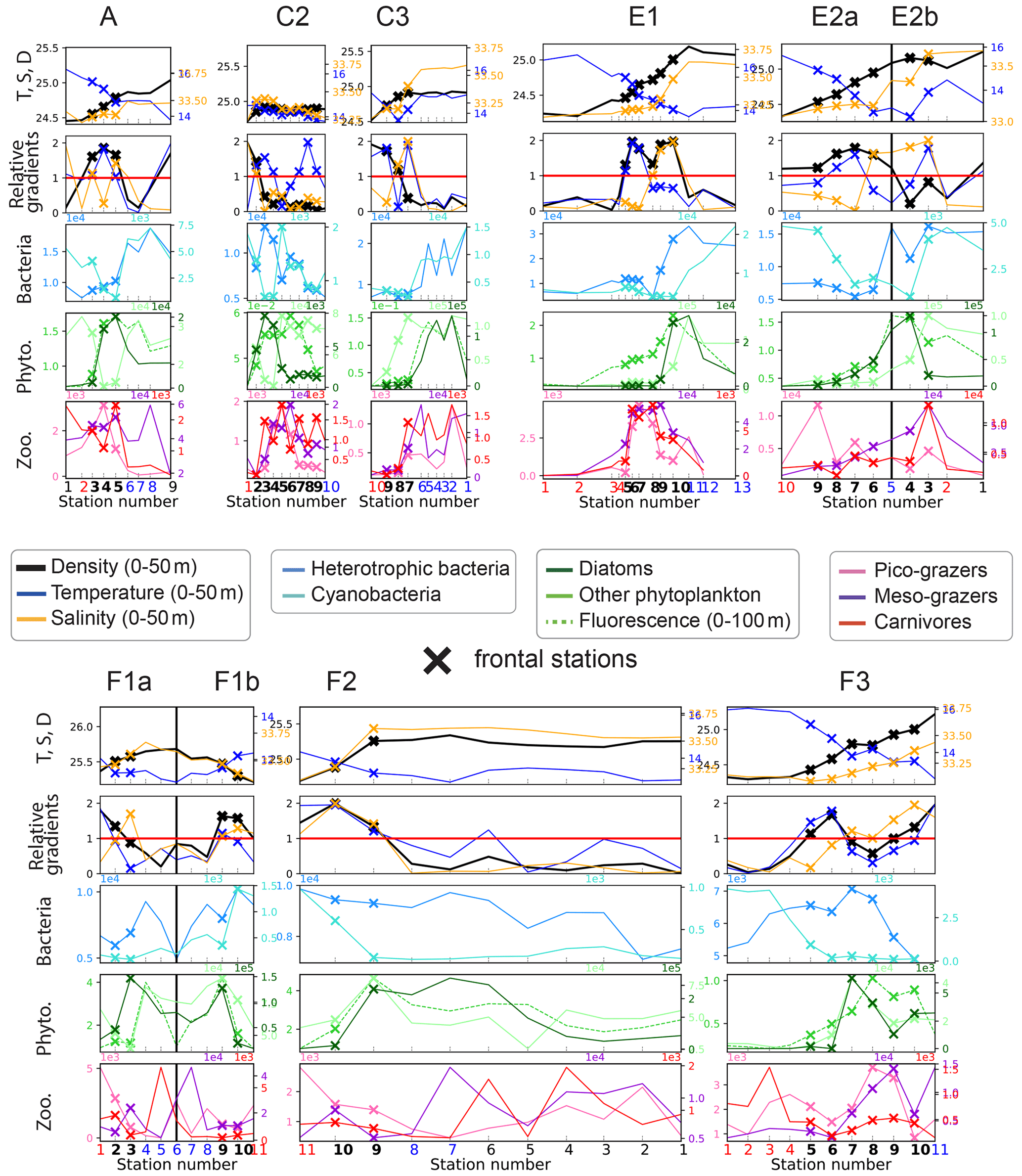
Figure 4First row: distribution of density (kg m−3), temperature (∘C), and salinity (PSU). Second row: density, temperature, and salinity relative gradients. Third, fourth, and fifth rows: biomass (µgC m−3) of the seven plankton groups and fluorescence, along the eight transects. Frontal stations are represented with crosses, and the station number is shown at the bottom of each panel in bold for frontal stations, red for warm background stations, and blue for cold background stations. The center of the filaments in transects E2 and F1 is indicated with a black vertical line. The relative gradient threshold used to define frontal stations is indicated with a red horizontal line. The same scale is used along the x axis for all transects. The same grid spacing is used along the y axis for density, temperature, and salinity across all transects; different scales are used for biomass.
3.1 Biomass enhancement at fronts
3.1.1 Variability between fronts
We find that while plankton communities are generally enhanced at fronts, this effect is not uniform across either the plankton groups or the fronts. In particular, front C3 (Fig. 5) represents an extreme case with no frontal enhancement of the total biomass and the majority of individual taxa. Such fronts are deemed “transition fronts” in contrast with the “peak fronts” that do have an enhanced frontal community with maxima of the total phyto- or zooplankton.
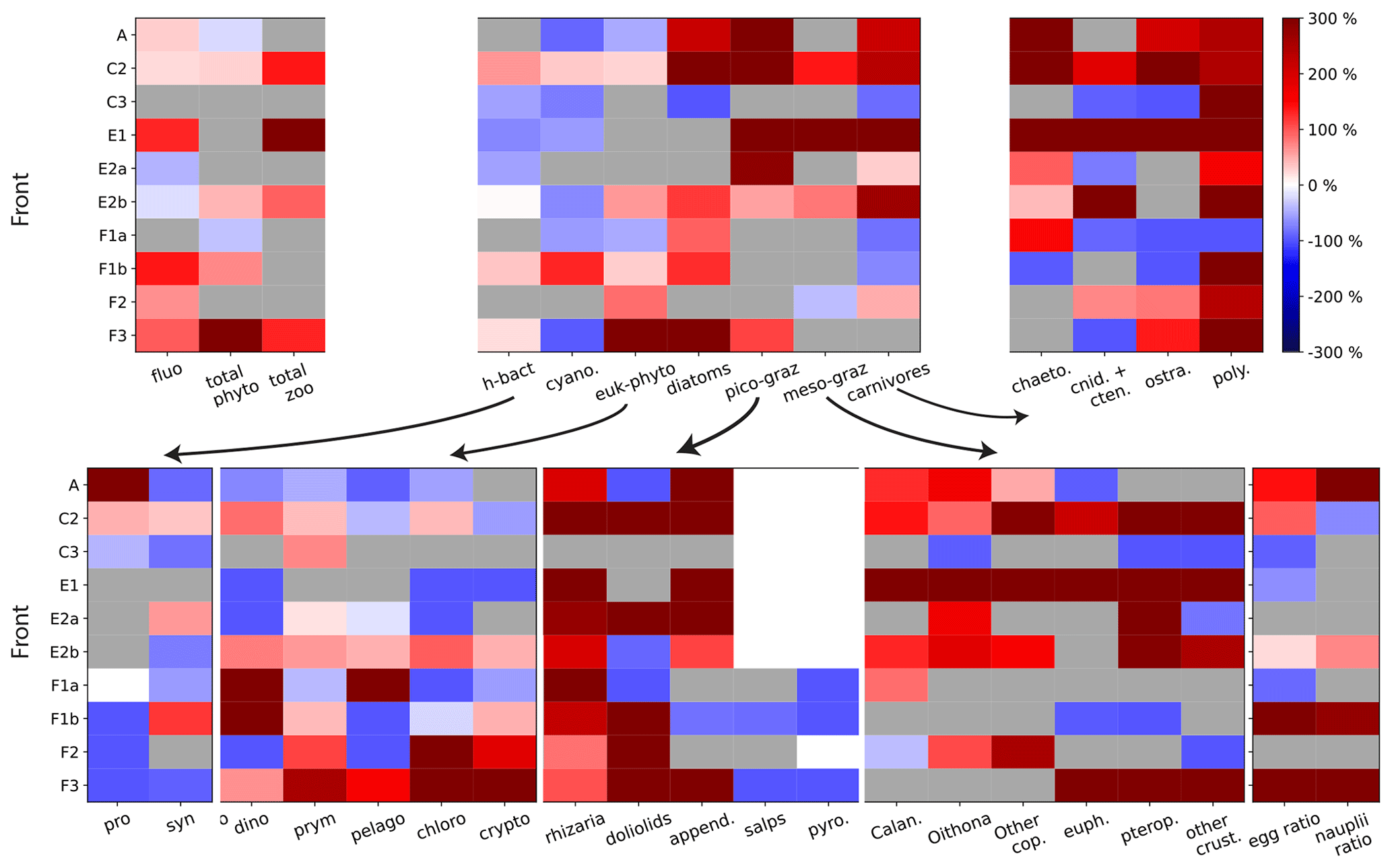
Figure 5Front enhancement factor of the plankton community for the 10 fronts sampled. Grey boxes indicate transition fronts: in such cases there is no enhancement at the front and the factor is undefined. Red and blue boxes indicate the intensity of the enhancement at the front: a species more abundant at the front than in the background is shown in red (positive enhancement factor); a species less abundant at the front than in the background is shown in blue (negative enhancement factor). The 10 fronts are organized along the y axis and the plankton taxa along the x axis. The first panel (upper left) shows the total biomass for phytoplankton, for zooplankton, and the fluorescence. The second panel (upper middle) shows the seven functional groups. The other panels show the individual taxa constitutive of each group. The last panel (bottom right) shows the early stages of copepods and euphausiids.
We find that some trophic groups have more consistent behaviors than others: diatoms and picograzers are almost always strongly enhanced at every front, heterotrophic bacteria and other phytoplankton are generally weakly enhanced, while mesograzers and carnivores are only occasionally strongly enhanced (Fig. 5, upper middle panel). However, the examination of these changes at a finer taxonomical resolution reveals that only a few of the taxa constituting these groups (such as diatoms, copepods, rhizarians, appendicularians, chaetognaths, and polychaetes) are systematically enhanced. Most of the other zooplankton taxa have very intense peaks at only a few fronts (doliolids, euphausiids, pteropods, other crustaceans, cnidarians, and ostracods), while the responses of the rest of the phytoplankton (diatoms excepted) tend to be more variable (alternatively increasing or decreasing depending on the front) and less intense (Fig. 5, upper right and lower panels).
3.1.2 Modification of the taxonomic structure at peak fronts
At peak fronts, there is a maximum of either Chl-a fluorescence or total phyto- or zooplankton biomass (Fig. 5, upper left panel). However, the behavior of the individual trophic groups is not always that of the total, which implies that the signal of the total biomass can mask differences at finer taxonomical resolution. In some cases, the differences are simply in the intensity of the enhancement: for instance, at front C2, diatoms have a much stronger response than the other phytoplankton types (Fig. 5). In other cases, however, different groups can have divergent behaviors. For instance, at front F3, the enhancement of the total phytoplankton (Fig. 5 upper left panel) masks a minimum of cyanobacteria (Fig. 5 lower left panel), which represent less than 0.1 % of the total biomass. At the A-front, the total zooplankton signal (“transition”) is dominated by the most abundant group, the mesograzers, whose “transition” masks the peaks of the picograzers and carnivores. Still in the A-front, the weak signal of the total phytoplankton is the balance of the much stronger positive and negative enhancements of diatoms and the other phytoplankton, respectively.
At an even finer taxonomical resolution (Fig. 5, top right panel and bottom row panels), the signal of a trophic group can also mask differences between the individual constituent taxa. This is particularly important because taxa belonging to the same trophic group have similar ecological roles and are expected to have similar responses to variations of their food supply. For instance, in the A-front, copepods and euphausiids have a maximum and a minimum, respectively, despite the fact that both of them can consume diatoms (which also exhibit a maximum). The implications in terms of the driving processes will be discussed in the Discussion section.
3.2 Cross-frontal patchiness
In this section, we examine whether biomass peaks are aligned with the density gradient or shifted toward the warm or the cold side of the front. We investigate the variability across fronts and across plankton taxa: are the peaks of all taxa aligned with the density gradient peak? Does a single taxon have peaks with similar characteristics for all the fronts?
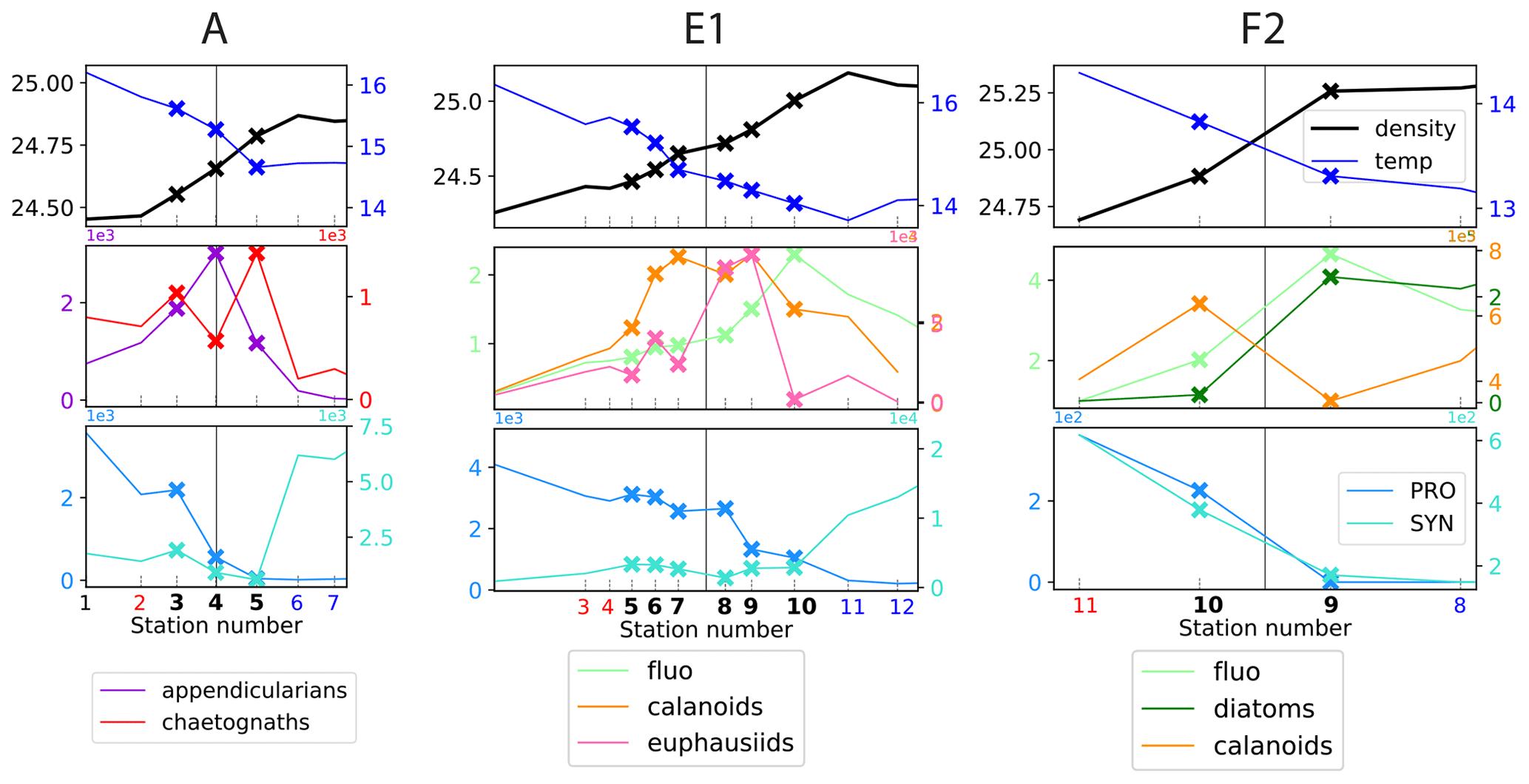
Figure 6Distribution of physical and biological properties across three of fronts. The first row shows the physical structure of the fronts (temperature and density). The second row illustrates the fine-scale spatial variability of the biomass peaks among two functionally different taxa (chaetognaths and appendicularians, A-front), among functionally similar taxa (calanoid copepods and euphausiids, E1), and among prey and predator taxa (fronts E1 and F2). The third row illustrates the segregation of cyanobacteria on either side of the fronts (“transition”). Frontal stations are indicated by crosses; the stations on the warm and cold side are shown in red and blue, respectively. The vertical line shows the middle of the frontal stations, defined with the density gradient. The same grid spacing is used for the x axis of the three fronts.
Examination of the data along all high-resolution transects reveals that there is variability at a very fine scale (up to 1–2 km), i.e., between consecutive stations: in a single transect, biomass peaks of different taxa frequently occur at different stations, occur on different sides of the front, and have different widths (Figs. 6, A11, A12, and A13). Importantly, these different patterns among taxa concern taxa with a variety of ecological relationships, including prey–predator, competitors (i.e., taxa with similar ecological roles belonging to the same functional group), and taxa with no direct interaction. These three cases are illustrated in Fig. 6 with diatoms–calanoid copepods and diatoms–euphausiids for the prey–predators (fronts E1 and F2, middle and right panel), calanoid copepods–euphausiids (both mesograzers that consume large phytoplankton) for the competitors (front E1, middle panel), and appendicularians–chaetognaths for the taxa with little direct interaction (A-front, left panel). In all of the cases, the peaks differ in location and widths.
Figure 7 compares the position and width of the biomass peaks and density gradients for each front and each taxon. We find that wide physical fronts (such as E1 and F3, 20–30 km wide) can be associated with both narrow and wide biomass peaks, while narrow fronts (such as A and C2, 5–15 km wide) tend to be associated with narrow biomass peaks. Importantly, the physical scale of the front (width of the density gradient peak) is always wider than the biological scale of the fronts (width of the biomass peaks). The position of the biomass peaks is highly variable depending on the front. Over most fronts, plankton taxa are shifted toward the cold side (fronts A, E1, F1a, F1b, F3), but over fronts C2 and E2b they are shifted toward the warm side, and in one case (F2) taxa are evenly split between the warm and cold side. Furthermore, individual taxa do not have systematic behaviors; they can peak on the warm or cold side and have wide or narrow peaks, depending on the front.
It should also be noted that some biomass peaks are shifted so far from the density gradient peak that they are located among the background stations. These peaks (such as the diatom peak in front E1 or the fluorescence peak in front F1a) were thus missed entirely in the computation of the peak enhancement factor.
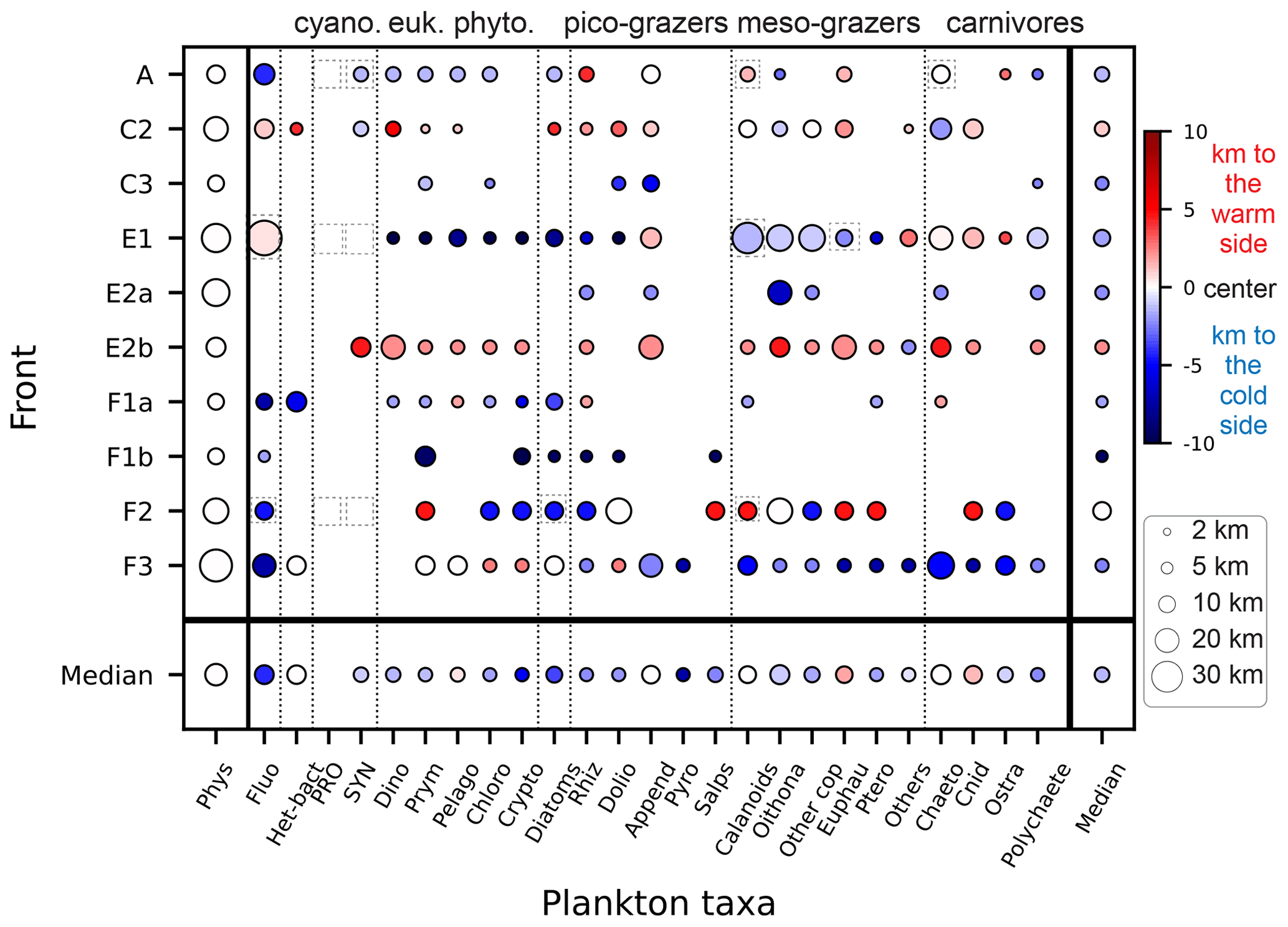
Figure 7Size of the plankton biomass peaks, relative to the size of the front in the cross-front direction. The color scale indicates the position of the biomass peaks relative to the center of the physical gradients (km): positive values (red) mean that the biomass peak is shifted toward the warm side of the front, and negative values (blue) mean that the biomass peak is shifted toward the cold side of the front. The size of the circle indicates the width of the peaks. The absence of a circle indicates the lack of a biomass peak (“transition” behavior). Dashed squares highlight the taxa presented in detail in Fig. 6.
4.1 How common are biomass enhancements at fronts?
We find that 7 out of the 10 fronts included in this meta-analysis are associated with an enhanced biomass of phytoplankton and zooplankton, showing that fronts are generally more than simple barriers between plankton communities and often support a specific frontal plankton community. This is consistent with a glider study of 154 fronts in the CCE-LTER region, where Powell and Ohman (2015) found frequent front-related enhancement of Chl a and mesozooplankton acoustic backscatter. However, it is possible that these “peak fronts” are over-represented in this dataset because the cruises specifically targeted intense and stable structures that are the most likely to be associated with a strong ageostrophic circulation and thus with biomass enhancements. A counter-example to our finding was presented by Tzortzis et al. (2021), who investigated the biological effect of less energetic fronts in the Mediterranean Sea and found that they were mostly boundaries between distinct phytoplankton taxa.
The detected biological enhancements over CCE-LTER fronts were made possible by the high across-front resolution of the sampling. Indeed, horizontal spacing between two adjacent stations along the CCE-LTER transects resolved cross-frontal patchiness, with only the coarsest transect (F2, resolution of 8 km, Fig. 6c) at the limit. Our results clearly showed that biomass peaks are thinner than the front and could have easily be missed with a coarser sampling. However, it is also possible that structures at an even finer cross-frontal scale exist: for instance, Chekalyuk et al. (2012) showed the presence of a patch of Synechococcus only 100 m wide in the A-front using continuous shipboard measurement that was missed in the CTD transect.
One limitation of the CCE-LTER dataset is that HPLC samples were only analyzed at the surface for most of the fronts, which did not allow the detection of peaks when they were in the subsurface. Nevertheless, Chl-a fluorescence measurements, which were conducted continuously during each CTD profile, provided useful and complementary information on the vertical structure of phytoplankton despite their low taxonomic resolution. For example at front F2, there was no visible HPLC-surface diatom peak, but there was a peak in the vertically integrated Chl-a fluorescence (right panel in Fig. 6), suggesting that the biomass enhancement was likely in the subsurface. In other cases, we noted that some of the phytoplankton peaks detected by surface measurements were horizontally shifted from the vertically integrated values of both zooplankton and Chl-a fluorescence (e.g., fronts E1 and F3). Indeed, vertical profiles of Chl-a fluorescence revealed that chlorophyll layers were tilted (Fig. A5), which can explain both the horizontal shift and the wider scale of the vertically integrated peaks. Tilted layers are commonly found in frontal structures and are indicative of the vertical ageostrophic circulation generated during frontogenesis (de Verneil et al., 2019). In addition, a finer vertical resolution than achieved in CTD transects might be necessary to fully resolve the vertical structures. Indeed, the use of the MVP at the E-front revealed the presence of very fine vertical layers (1–10 m) in the chlorophyll a and salinity distributions (de Verneil et al., 2019) that were only partially resolved with the Niskin bottle data, which were collected with a vertical resolution of 10–20 m). Moreover, the use of an in situ imaging system in towed instruments similarly revealed heterogeneities in the zooplankton distribution at scales of a few meters (Ashjian et al., 2001).
The dataset used in the present study provides a snapshot view of the planktonic ecosystem but cannot capture their time evolution. Thus, our estimates of frontal enhancement might not be representative of the mean amplification over a longer period of time. Spatiotemporal variability at fronts may result from three factors: first, frontal communities may not be at equilibrium because the nutrient supply is intermittent. For example, the C3-front does not have a biomass enhancement despite the presence of a very intense density gradient. One explanation for this paradoxical situation is the delay between the onset of the nutrient injection and the accumulation of phytoplankton and zooplankton biomass. If the transect had been conducted a few weeks or maybe even a few days later, biological enhancements might have been detected.
Second, fronts are constantly being displaced by the horizontal circulation (which is particularly intense in the CCE), and their location can change quickly and unpredictably. It is thus difficult to follow the evolution of a front over a few weeks. The 2012 cruise attempted to do this by performing two transects (E1 and E2) at the same coordinates 2 weeks apart. However, the physical seascape shifted in the interval because of the unexpected arrival of a coastal filament, which resulted in two different structures being sampled in the two transects (Fig. A3 and video supplement, Mangolte, 2023d). This example highlights the need to follow in real time the evolution of water masses before choosing the location of a transect. This requires real-time Lagrangian analysis of satellite data (e.g., using the SPASSO software as in Tzortzis et al., 2021; Rousselet et al., 2018; Barrillon et al., 2023).
Third, water is advected quickly along the fronts: frontal jets often have velocities of 0.5 m s−1, i.e., about 50 km d−1 (Barth et al., 2000; Kosro and Huyer, 1986; Zaba et al., 2021). The composition of a plankton community at a given transect site thus depends on the conditions upstream of the front and the history of the water masses. Specifically in the CCE, the horizontal circulation connects fronts with the coastal upwelling zone, whose intensity strongly varies over only a few days. These short upwelling pulses can generate chlorophyll patches that are then advected away from the coast by mesoscale eddies and frontal jets and can result in along-front patchiness (Gangrade and Franks, 2023).
4.2 What are the implications of the observed taxonomic structure for the driving processes?
In “transition fronts”, the composition of the frontal community can be explained by simple cross-frontal mixing between communities on the warm side and cold side, respectively. In contrast, the specific community encountered in “peak fronts” requires additional processes capable of selectively increasing the biomass of some groups, such as local growth, transport from a more productive region, and/or biotic interactions (Fig. 8).
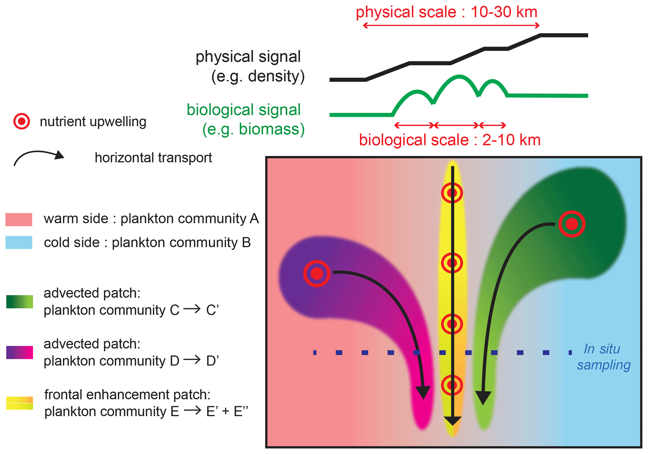
Figure 8Schematic representation of the processes driving changes in community structure and fine-scale cross-frontal patchiness at fronts. Black and green lines on the top of the figure show the cross-front distributions of density and biomass; the physical signature is generally wider than the biological peaks, although the density or temperature gradients can increase in small steps. The green and purple plankton community mature as they are transported by horizontal currents and converge at the front. Nutrient injections at the front stimulate plankton growth; the different conditions experienced by plankton (nutrient supply, light, temperature, biotic interactions) can create different communities toward the warm (yellow to green gradient) or cold side (yellow to orange gradient).
We found that the enhancement of total biomass is associated with a modification of community structure. This implies that different taxa respond in different ways to frontal dynamics. In particular, we examined the behavior of rarer taxa that are masked by the dominant groups when only the total chlorophyll or the total particle count is measured. Importantly, we found that two taxa with similar ecological roles within a trophic group can have different responses at fronts. We found that many taxa of both phytoplankton and zooplankton are almost systematically associated with fronts. While this behavior is well-known for some (particularly diatoms, Franks, 1992; Claustre et al., 1994; Yoder et al., 1994; Allen et al., 2005; Ribalet et al., 2010; Carreto et al., 2016; copepods, Boucher, 1984; Thibault et al., 1994; Derisio et al., 2014; Ohman et al., 2012; and gelatinous zooplankton, Graham et al., 2001; Luo et al., 2014), the effect of fronts on other taxa has only been investigated very occasionally (e.g., Capitanio and Esnal, 1998, for appendicularians).
The most intuitive explanation for the high abundance of these groups is increased growth in response to the supply of nutrients. In order to test this relationship, we attempted to characterize the age of the fronts, which we assumed to be a proxy of the duration of the supply of nutrients by the ageostrophic circulation. Most of the fronts included in this analysis are relatively stable, and the physical structures underlining them (SST or SSH gradients and FSLE ridges) are generally visible on satellite images at least a few weeks before each transect was conducted, depending on the cloud cover (video supplements, Mangolte, 2023b, c, d, e). Such timescales, in principle, are long enough to support the local growth of phytoplankton (Lewandowska et al., 2015) and most mesozooplankton (Kotori, 1999; Bouquet et al., 2018; Eiane and Ohman, 2004). However, the cloud cover, the complexity of the structures, and their spatial movement make it difficult to precisely date the appearance of the gradients identified in the transects. It should also be noted that injections of nutrients at fronts should only produce an increase of the growth rates if the phytoplankton population is nutrient-deprived, which is not the case for every front (Fig. A10). Interestingly, however, the “younger” fronts (F1–F2, which can only be identified on satellite images for a few days before the transects) show less zooplankton enhancement than the other fronts. The zooplankton taxon with the fastest reproduction rate, the appendicularians, is also the one most strikingly enhanced at fronts (Fig. 5). But despite these observations, a robust causal link is difficult to establish because of the many large uncertainties associated with both the estimation of “frontal age” and biological growth rates, particularly the reproduction rates of zooplankton, which are highly variable at taxonomical resolutions finer than the present dataset. Finally, we cannot rule out the possibility that peaks of both biomass and secondary production are attributable to advection along the front of a more productive water parcel. Community structure not only depends on the local frontal dynamics, but it is also strongly influenced by the regional context, which in our study region is dominated by the coastal upwelling. Consequently, the description of these local dynamics alone is not sufficient to explain the community structure. Instead, the elucidation of the relative importance of these two processes (frontal injections of nutrients and advection) requires taking into account the history of the water parcels by adopting a Lagrangian perspective (Gangrade and Franks, 2023).
Finally, the third process – biotic interactions – may explain some of the differential responses among plankton groups. Indeed, we found that many phytoplankton taxa other than diatoms often have lower abundances at fronts than in their surroundings. A recent modeling study offers a possible mechanism that could explain this observation: Mangolte et al. (2022) showed how two competitive processes can be intensified by frontal conditions, resulting in lower abundances of cyanobacteria and coccolithophores: community shading (reduced growth rate because of light competition with another phytoplankton group located higher in the water column) and shared predation (increased grazing losses because of a shared predator with another group). However, it should be noted that the decrease of some of the phytoplankton groups was not shown in additional measurements made in the A-front with a different methodology (epifluorescence microscopy). The minima of prymnesiophyte and dinoflagellate HPLC-derived biomass were either very reduced or absent from the microscopy measurements (Fig. A8). One explanation is that the pigment composition of these groups was different at the front, possibly as a result of a change at the species level, and was interpreted as a lower abundance by the HPLC methodology (which relies on the assumption of a constant pigment composition). Another explanation is that the cell counts produced by the epifluorescence microscopy semi-automated system underestimated the abundance of these groups outside the front, possibly also as a result of a modification of the species assemblage at the front. Both explanations suggest that a higher level of taxonomical resolution (up to the species level, for instance provided by genomics) may be necessary to go further in our understanding of the effect of fronts on phytoplankton communities.
In the case of cyanobacteria, a shared predation mechanism involving heterotrophic bacteria as the competing prey and nanozooplankton (heterotrophic nanoflagellates and ciliates) as the common predator was introduced by Goericke (2011) and later termed the “enhanced microbial loop” by Taylor and Landry (2018). In these studies, this mechanism was invoked to explain large-scale patterns of phytoplankton community structure (for instance between productive coastal waters and oligotrophic offshore waters at scales of hundreds of kilometers); here we suggest that it could also play a role at much smaller scales (1–10 km; i.e., between productive frontal waters and an oligotrophic background). In the enhanced microbial loop framework, the elevated particulate organic carbon concentration (such as detritus or faecal pellets) and associated microbial activity lead to an increase of nanoflagellate predation on both heterotrophic and cyanobacteria, ultimately resulting in a decrease of the abundance of cyanobacteria. Indeed, Samo et al. (2012) showed that the growth of heterotrophic bacteria is elevated in the A-front and attributed the absence of a similarly elevated biomass to viral lysis. We also suggest that the shared predation could be mediated by appendicularians in addition to nanozooplankton. Appendicularians are also likely to play a particularly important role in the top-down regulation of bacteria because their extremely high growth rates allow them to react quickly to an increase in their food supply (Capitanio and Esnal, 1998). Many of the other fronts in our meta-analysis similarly have a moderate increase of bacteria and a very high increase of appendicularians; however the omission from the measurements of nanozooplankton (heterotrophic nanoflagellates and ciliates) prevents us from drawing conclusions on the relative importance of the two trophic pathways, limiting our understanding of the biotic processes regulating plankton communities at fronts.
Thus, in the CCE-LTER fronts, the plankton community structure is likely regulated by the coupling of transport and biotic interactions, including both bottom-up (growth in response to nutrient injections) and top-down (elevated grazing pressure) processes.
4.3 What are the implications of the observed spatial structure for the driving processes?
We found that there is cross-frontal patchiness at scales smaller than the front (Fig. 8): biomass peaks (2–10 km) are narrower than physical fronts (10–30 km), and they are shifted toward the cold side (more commonly) or the warm side by up to 10 km. Furthermore, the peaks of different plankton taxa can have different positions along the transect and different widths.
The fine-scale cross-frontal patchiness suggests that there are processes capable of spatially decoupling the biomass of different plankton taxa, creating multiple adjacent communities rather than a single “frontal plankton community”. Importantly, the spatial decoupling affects closely interacting taxa (such as competitors and prey–predators) that are expected to remain together in a purely bottom-up scenario.
Therefore, additional processes, such as advection by currents and biotic interactions, are necessary to explain the observed patchiness. Two scenarios could explain how such different communities could be located in such proximity (Fig. 8). First, these communities could have been generated in remote locations and brought together by the converging horizontal circulation. The different taxonomic structures would be caused by the different environmental conditions (such as the date and intensity of the nutrient supply) experienced by the water masses. The analysis of water mass trajectories supports this scenario at the E-front (de Verneil et al., 2019), while a cursory examination of satellite data suggests that this is also the case in some of the other fronts in this analysis (most notably C2; Fig. A2).
Second, an initially homogeneous frontal community could have evolved in different ways because of differences in the environmental conditions across the frontal gradient. These differences could involve the nutrient supply: the frontal injection of nutrients is theoretically located on the warm side because of the direction of the ageostrophic frontal circulation. However, the exact location of the nutrient supply is difficult to determine from the data because the center of the density gradient is not necessarily a good proxy for the center of the ageostrophic circulation. In addition, meanders of the fronts can create a geostrophic pumping of nutrients on either side (Oguz et al., 2015; Lohrenz et al., 1993).
They could also be related to differences in stratification and temperature, which can influence a variety of biotic processes from the growth rates of phytoplankton to the diurnal vertical migration (DVM) of zooplankton and the prey–predator encounter rates. The patchiness can be maintained at a very fine scale (a few kilometers) as long as the timescale of these biological processes is faster than turbulent mixing.
Despite the richness of this dataset, there is not enough information on the potential drivers to quantify the contribution of each process. For instance, the elucidation of biotic interactions requires knowledge of nutrient fluxes and growth and grazing rates, not just the nutrient stocks and abundances. In addition, given the intensity of the mesoscale circulation, knowledge of the conditions upstream of the fronts is needed. Even with the information that is available, there are significant uncertainties, particularly for the age and location of the frontal supply of nutrients (detailed above). Furthermore, interactions among different drivers need to be taken into account.
In this study, we describe the taxonomic structure and fine-scale spatial organization of plankton communities across 10 fronts in the California Current Ecosystem upwelling region. The hypothesis of frontal nutrient injections explains the predominance of diatoms at fronts, but it needs to be supplemented by other processes (i.e., biotic interactions and transport) to explain the differential responses of the other plankton groups and the cross-frontal patchiness. The high horizontal and taxonomic resolution of our dataset allowed us to gain a more complete view of fronts as complex structures driven by the coupling of physical and biological processes. The understanding of the role of fronts on marine ecosystems by empirical means can be further improved in two ways. Firstly, frontal communities should be sampled at appropriate horizontal, vertical, taxonomic, and temporal resolution. While many instruments can achieve excellent performance at one scale, the challenge lies in simultaneously increasing all the dimensions of resolution, which can be achieved by strategically combining multiple shipboard and autonomous instruments. Secondly, the quantification of the role of the key processes at fronts requires the adoption of a Lagrangian perspective to follow the evolution of the community as it is advected by the currents, which should include in situ biological rates (growth and grazing) along the drifter trajectory combined with high-resolution altimetry measurements to characterize the regional circulation.
The elucidation of the structure of frontal ecosystems and of the processes driving them should then allow the development of parametrizations that will permit fronts to be included in global climate models and fishery management models in order to ultimately evaluate their contributions to the cycling of matter and energy in the ocean.
The following sections describe the regional context of each of the four cruises and the physical structure of each transect. We present the transect CTD data (Fig. 4 and vertical distribution in Fig. A9), and we reconstitute the evolution of the frontal structures in the weeks before and after the transect date by visually examining satellite data (Figs. A1, A2, A3, and A4 and video supplements, Mangolte, 2023b, c, d, e).
A1 A-front
In October 2008, an SST front named “A-front” was identified and sampled in a single 25 km transect consisting of nine stations spaced about 3 km apart. The data from this transect, along with other measurements taken during the cruise, were extensively analyzed (including the physical and ecological properties of the front, from bacteria to fishes) and published in a series of papers (see Landry et al., 2012, for a summary of the results).
Transect A crossed an isolated, narrow front (the A-front), clearly marked by steep density and temperature gradients at stations 3, 4, and 5 (forming a front about 5 km wide; Fig. 6a). It separates warm waters on the south side (stations 1 and 2) from colder waters on the north side (stations 6, 7, and 8). The A-front is located just north of the California Current, which is characterized by a subsurface minimum of salinity visible in station 1 (Fig. A9). Satellite data (SST and water age) show that the A-front was sharpened about 3 weeks before the transect was conducted, when the arrival of a mass of upwelled water from the north suddenly intensified the north–south temperature gradient (Fig. A1 and video supplement, Mangolte, 2023b). An anticyclonic eddy also developed on the south side of the front as the gradient intensified. In situ velocity data and the results of numerical simulations showed that the A-front is associated with an eastward, along-front geostrophic current and a vertical cross-frontal ageostrophic circulation supplying nutrients to the euphotic zone (Li et al., 2012). The A-front is about 200 km long and remained nearly stationary for months after the cruise, suggesting that its ecological impacts could be significant.
A2 C-front
In July 2011, a frontal structure was identified and named the “C-front” because it crosses the California Current. Three transects were conducted: the first transect, C1, was initiated before the precise location of the front was known from the MVP survey and was quickly aborted because it did not adequately capture the front; it is not included in the present study. C2 and C3 were then conducted, and both include 10 stations over about 20 km, with a spacing of about 2 km. The distribution and biogeochemical properties of diatoms were investigated in Krause et al. (2015) and Brzezinski et al. (2015).
Transect C2 crossed a weak thermal front separating a warm-core anticyclonic eddy on the west (offshore) from colder waters on the east (inshore). The transect is relatively short compared to the width of the front and barely samples the cold and warm sides (Fig. A9). Notably, the temperature variation, although weak, is not uniform across the front: the temperature gradient is largest at stations 3 and 8, with a step of virtually constant temperature at stations 5, 6, and 7. Also notable, the temperature gradient is strongly compensated by the salinity, resulting in a low density gradient. The SST and SSH signature of the eddy are visible at least 3 months before and 3 months after the transect (Fig. A2 and video supplement, Mangolte, 2023c), suggesting that this frontal structure is relatively stable. Satellite data show the presence of a geostrophic current flowing south around the anticyclonic eddy, transporting water of coastal origin; the water age analysis shows that this water left the coast about 6 weeks before the transect.
Transect C3 crossed a very intense salinity front aligned with an extremely narrow cold filament (stations 7, 8, and 9), delimited by two thermal fronts at the filament's boundaries (Fig. A9). The complex salinity and temperature distributions lead to some thermohaline compensation (particularly at station 7), but a clearly defined density front is visible at stations 8, 9, and 10. The presence of clouds and the resolution of the satellite data make it difficult to identify precisely the structure sampled and the origin of the water. However, a reasonable hypothesis would be that a strong geostrophic front, driven by salinity, generated a horizontal current which advected the cold filament along the salinity front.
A3 E-front
In August 2012, a frontal structure at the boundary between two eddies, identified in SSH images, was named “E-front” (with E for eddy) and sampled in two transects, E1 and E2, which are both 50 km long and were conducted at the same coordinates 2 weeks apart. The resolution of E1 varies from 2 to 5 km, with stations more closely spaced in the center of the transect, while E2 has a constant spacing between stations of 5 km. The horizontal and vertical circulations at the E-front were investigated by De Verneil and Franks (2015), de Verneil et al. (2019), and Stukel et al. (2017) with a Lagrangian analysis and a model, respectively. Bednaršek and Ohman (2015) examined the distribution of shelled zooplankton across the front.
Transect E1 crossed a front in temperature and density between a warm anticyclonic eddy on the west (offshore) and a cold cyclonic eddy on the east (inshore). The frontal region is a wide area of steep temperature and density gradients (stations 5 to 10, with a width of about 20 km) separating warm, fresh water (stations 1–4) from cold, saltier water (stations 11–13). As noted by previous studies, the geostrophic jet flowing south along the front is the convergence of water masses of different origins, some from upwelling sites to the east and north of the transect zone and some from offshore (de Verneil et al., 2019; Gangrade and Franks, 2023). The water age analysis also shows water parcels of different origins in the frontal region, including some that left the coast 6 weeks before and some 10 weeks before the transect. This front is a relatively stable structure; the two eddies remain mostly stationary for about 2 months before and 1 month after the transects.
Despite being conducted only 2 weeks later at the same coordinates, the E2 transect crossed a different frontal structure because the two eddies and the E1 front were pushed offshore by the arrival of a coastal filament transporting recently upwelled water. This coastal filament (which is approximately 30 km wide) originated at an upwelling site east of the transect about 3 weeks earlier (Fig. A3 and video supplement, Mangolte, 2023d) and was transported counterclockwise around a cyclonic eddy located east of the transect. The cold filament is aligned with a very intense salinity front, which leads to some thermohaline compensation on station 3. However, two separate density fronts are visible, mainly driven by the two thermal fronts which separate the cold filament waters (stations 4, 5, and 6) from the warmer waters outside of it (9–10 and 1–2): front E2a (stations 6, 7, and 8) is the western edge of the filament, and front E2b (station 3) corresponds to its eastern edge. At the time of the transect, three water masses of different ages were present in the frontal region: young filament water (20 d old), older filament water (40 d old), and very old water trapped inside the eddy (3 months old). A likely scenario for the formation of this structure is the advection of recently upwelled water (the “young filament”) along the geostrophic salinity front.
A4 F-front
In June 2017, a coastal filament (the Morro Bay filament) transporting cold, recently upwelled, and productive water offshore (Zaba et al., 2021) was identified and three transects were conducted across it. The fronts separating the cold filament water and the warmer water around it are collectively named F-fronts. F1 is the closest to the shore, followed by F2 (10 d later), and then F3 (5 d later). F1 and F3 have a high resolution, similar to the previous cruises, while F2 is much longer and has a lower resolution of about 8 km.
Transect F1 crossed the entire filament and contains two fronts which correspond to the two edges of the filament: front F1a on the southern edge (stations 2–3) and front F1b (stations 9–10) on the northern edge. For both fronts, the cold side is the core of the filament (stations 4–8) and the warm side is outside the filament (stations 1 and 11). There is a complex thermohaline structure associated with the filament and the fronts, with steps in temperature that do not translate to the density structure, such that the frontal stations are better seen on the density structure.
Transect F2 also crossed the entire coastal filament. However, the front forming the southern edge of the filament (around stations 5–6) is weaker and compensated in density and was not included in the analysis. Stations 1–5 are part of an older filament which left the coast about 40 d before the transect (in contrast to the main filament, which left the coast less than 20 d before the transect). The F2 front thus corresponds to the northern edge of the main filament and is well defined by the elevated temperature and density gradients at stations 9, 10, and 11. The warm side is outside the filament (station 11), and the cold side is inside (stations 7–8).
Transect F3 crossed a wide region of strong temperature and density gradient (stations 5–11, 30 km width), corresponding to a transition between warm offshore waters (stations 1–5) and colder waters (station 11). These colder waters left the coast east of the transect 3 weeks before the F3 transect was conducted (Fig. A4 and video supplement, Mangolte, 2023e). Similarly to the C2 and F1a fronts, the temperature along F3 varies in steps, with stretches of flat gradient within the wide frontal region (in stations 7, 8, and 9). The FSLE and water age analysis suggest that this frontal region contains a narrow stirring filament transporting older coastal water (6 weeks) in a trajectory parallel to the main coastal filament. The secondary filament initially flowed southward but was pushed offshore by the main filament and was curved around it on the west side at the time of the F3 transect. The water of the secondary filament is older than the main filament (6 weeks vs. 3 weeks).
A5 Summary
In summary, this examination has revealed that all transects crossed temperature and/or density gradients (indicating the presence of a “front”), whose width varied between 5 and 30 km. In some fronts, the density varies in a single step (A, C3, E1, E2, F2). In the others (C2, F1, F3), the density varies in multiple steps, indicating the presence of structures at a scale smaller than the width of the front. Satellite data suggest that many of the fronts are associated with strong currents that advect filaments along the fronts. In some cases, multiple filaments converge in the frontal zone.
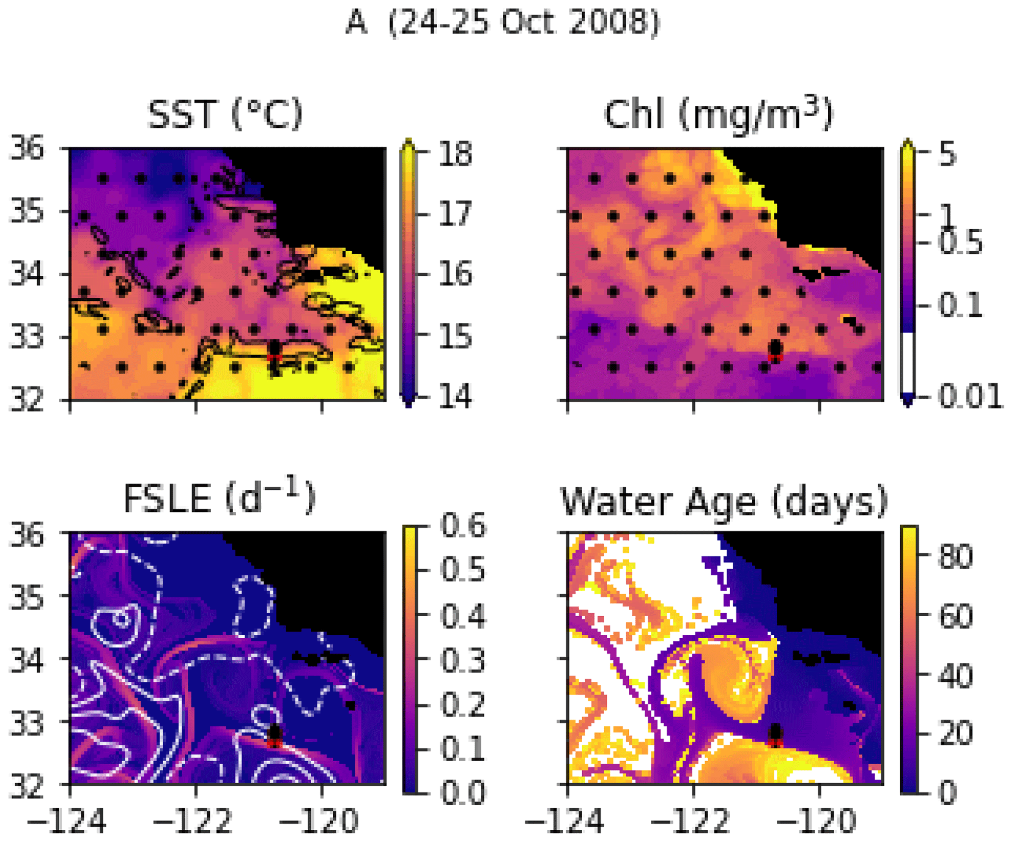
Figure A1Snapshots of satellite-derived data at the time of transect A: SST (black lines indicate SST fronts (HI > 10)), chlorophyll, FSLE (d−1, with SSH in white contours at 0, 0.05, 0.1, 0.15, 0.2, 0.25, and 0.3 m above geoid; dashed lines indicate cyclonic eddies and solid lines anticyclonic eddies), and water age (in days since the water parcel left the coast). The hatches indicate the presence of clouds, where the fields are smoothed by the interpolation (resulting in weaker gradients). The position of the transect is indicated with red crosses for frontal stations and small black dots for background stations.
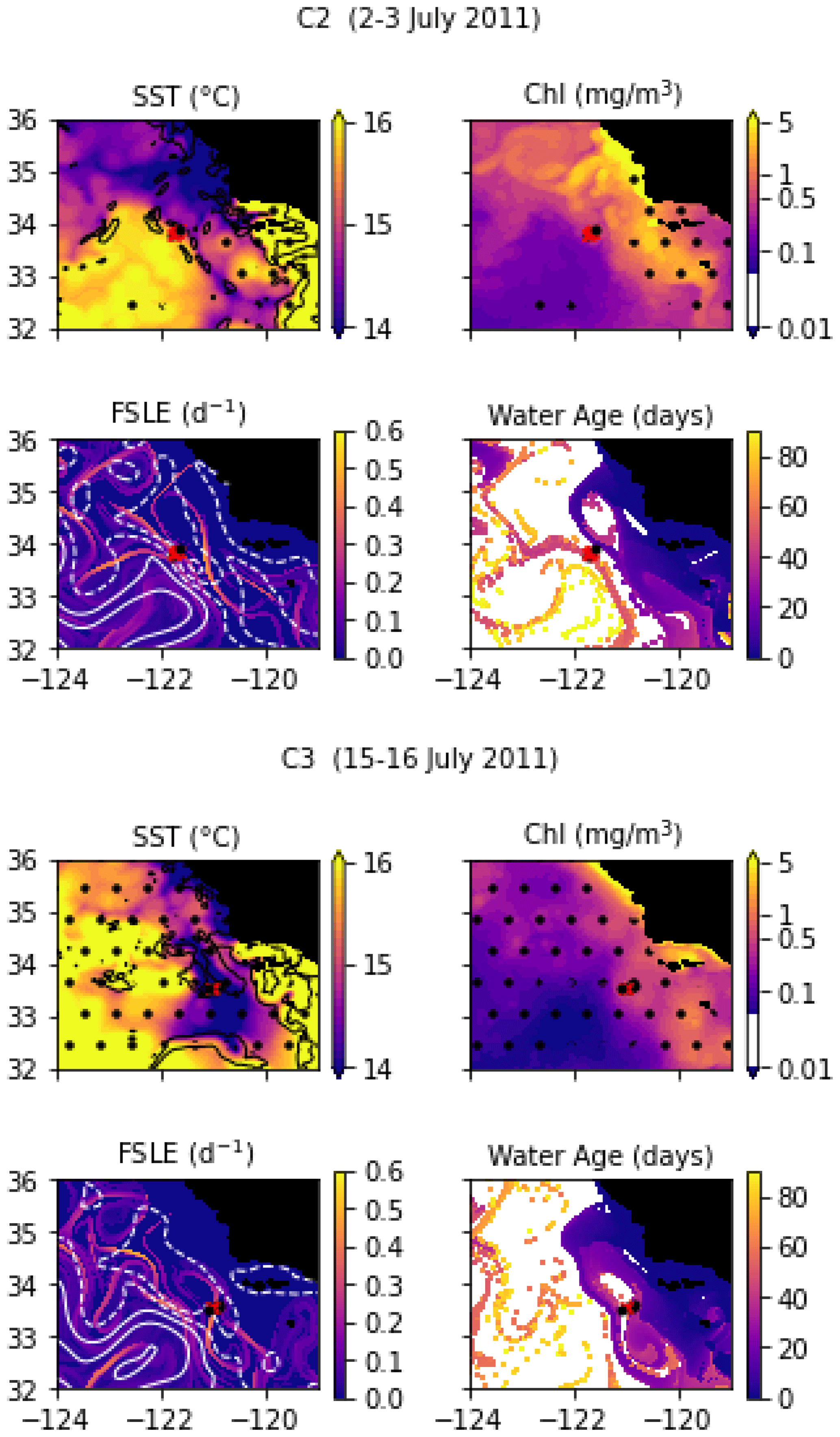
Figure A2Snapshots of satellite-derived data at the time of transects C2 and C3: SST (black lines indicate SST fronts (HI > 10)), chlorophyll, FSLE (d−1, with SSH in white contours at 0, 0.05, 0.1, 0.15, 0.2, 0.25, and 0.3 m above geoid; dashed lines indicate cyclonic eddies and solid lines anticyclonic eddies), and water age (in days since the water parcel left the coast). The hatches indicate the presence of clouds, where the fields are smoothed by the interpolation (resulting in weaker gradients). The position of the transect is indicated with red crosses for frontal stations and small black dots for background stations.
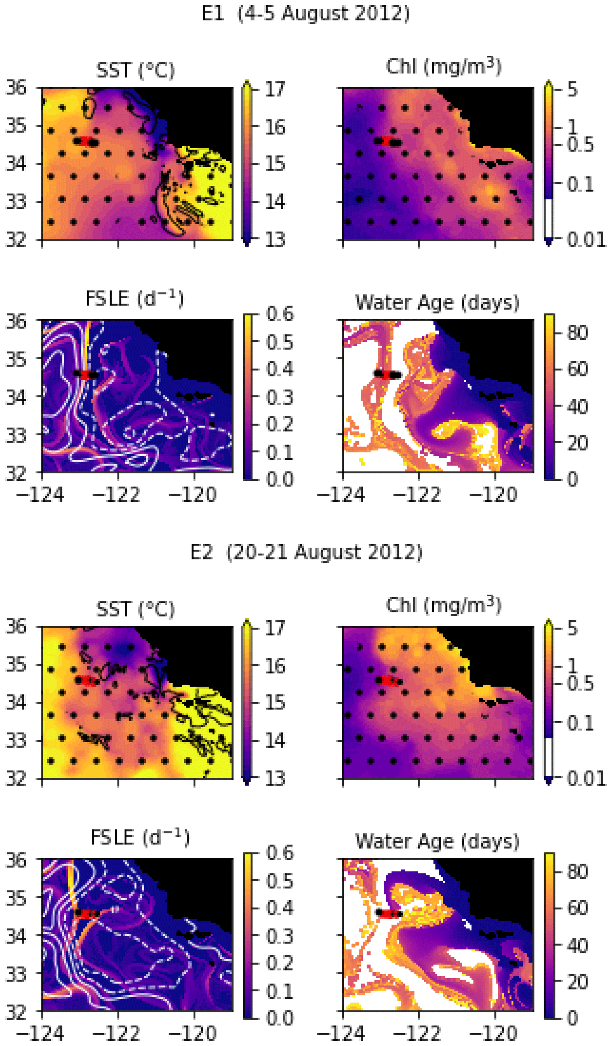
Figure A3Snapshots of satellite-derived data at the time of transects E1 and E2: SST (black lines indicate SST fronts (HI > 10)), chlorophyll, FSLE (d−1, with SSH in white contours at 0, 0.05, 0.1, 0.15, 0.2, 0.25, and 0.3 m above geoid; dashed lines indicate cyclonic eddies and solid lines anticyclonic eddies), and water age (in days since the water parcel left the coast). The hatches indicate the presence of clouds, where the fields are smoothed by the interpolation (resulting in weaker gradients). The position of the transect is indicated with red crosses for frontal stations and small black dots for background stations.
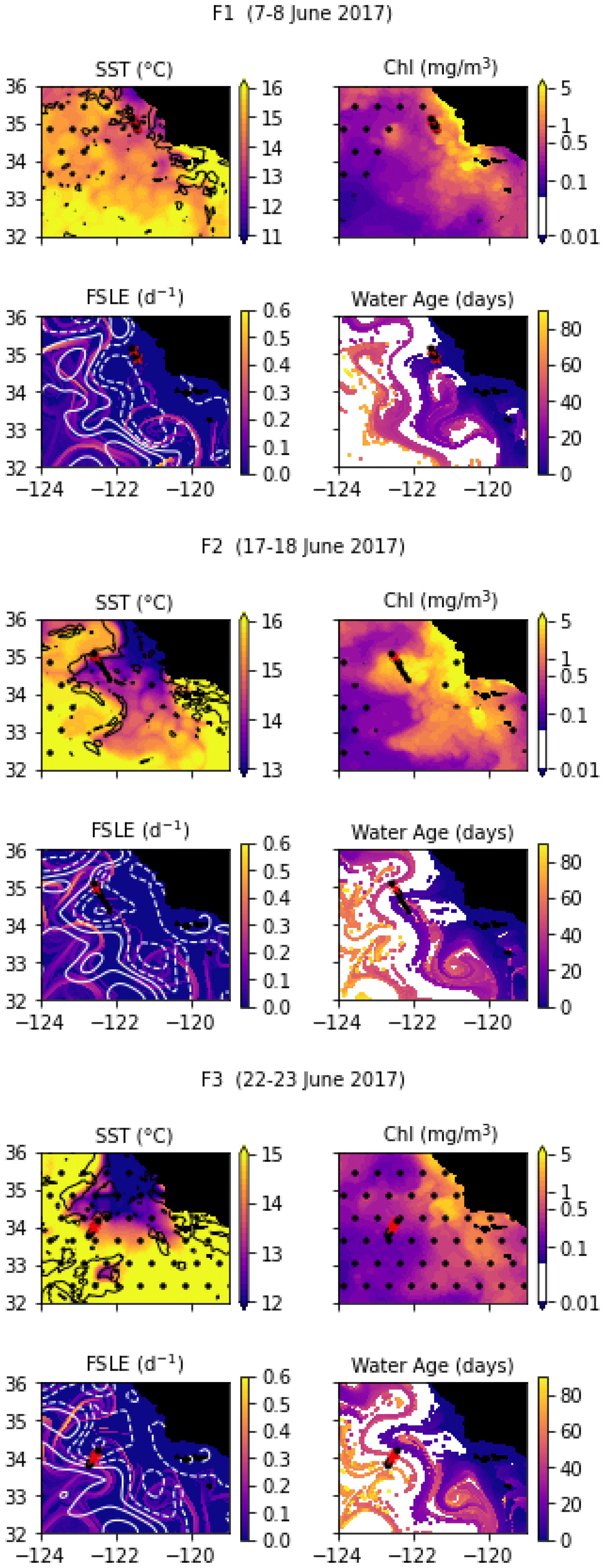
Figure A4Snapshots of satellite-derived data at the time of transects F1, F2, and F3: SST (black lines indicate SST fronts (HI > 10)), chlorophyll, FSLE (d−1, with SSH in white contours at 0, 0.05, 0.1, 0.15, 0.2, 0.25, and 0.3 m above geoid; dashed lines indicate cyclonic eddies and solid lines anticyclonic eddies), and water age (in days since the water parcel left the coast). The hatches indicate the presence of clouds, where the fields are smoothed by the interpolation (resulting in weaker gradients). The position of the transect is indicated with red crosses for frontal stations and small black dots for background stations.
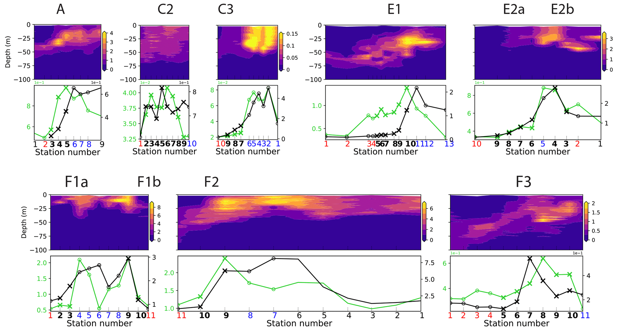
Figure A5Top row: vertical sections of fluorescence (V). Bottom row: vertically integrated fluorescence (0–100 m) and HPLC-derived surface Chl a (µg Chl a m−3). Front stations are indicated by crosses and the background stations by circles; the numbers of the frontal stations are shown in bold and the warm and cold sides in red and blue.
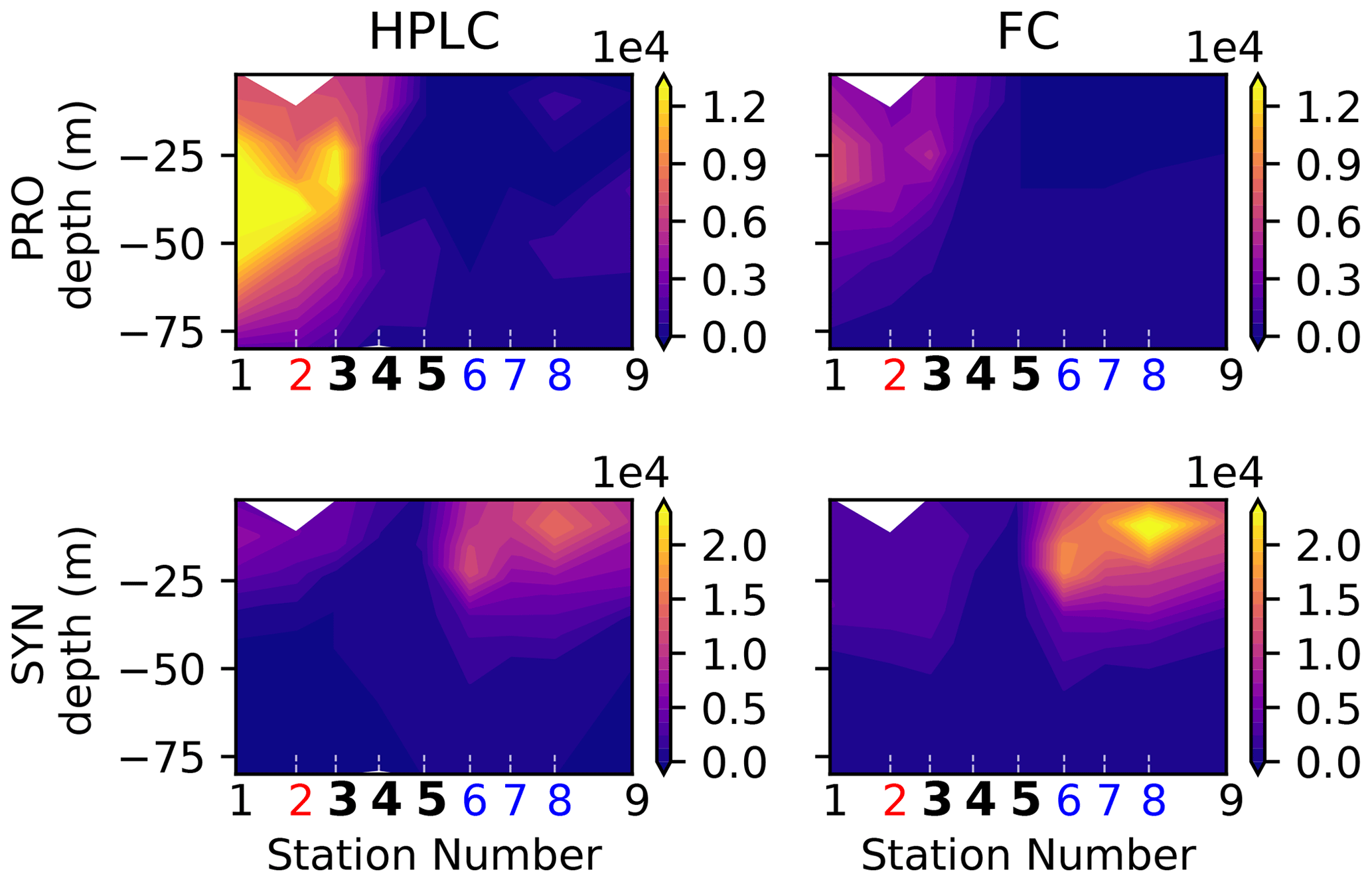
Figure A6Biomass (µgC m−3) of cyanobacteria (Prochlorococcus on the top row, Synechococcus on the bottom row) in the A-front transect measured by two different instruments: HPLC (left row) and flow cytometry (FC, right row). The numbers of the frontal stations are shown in bold and the warm and cold sides in red and blue.
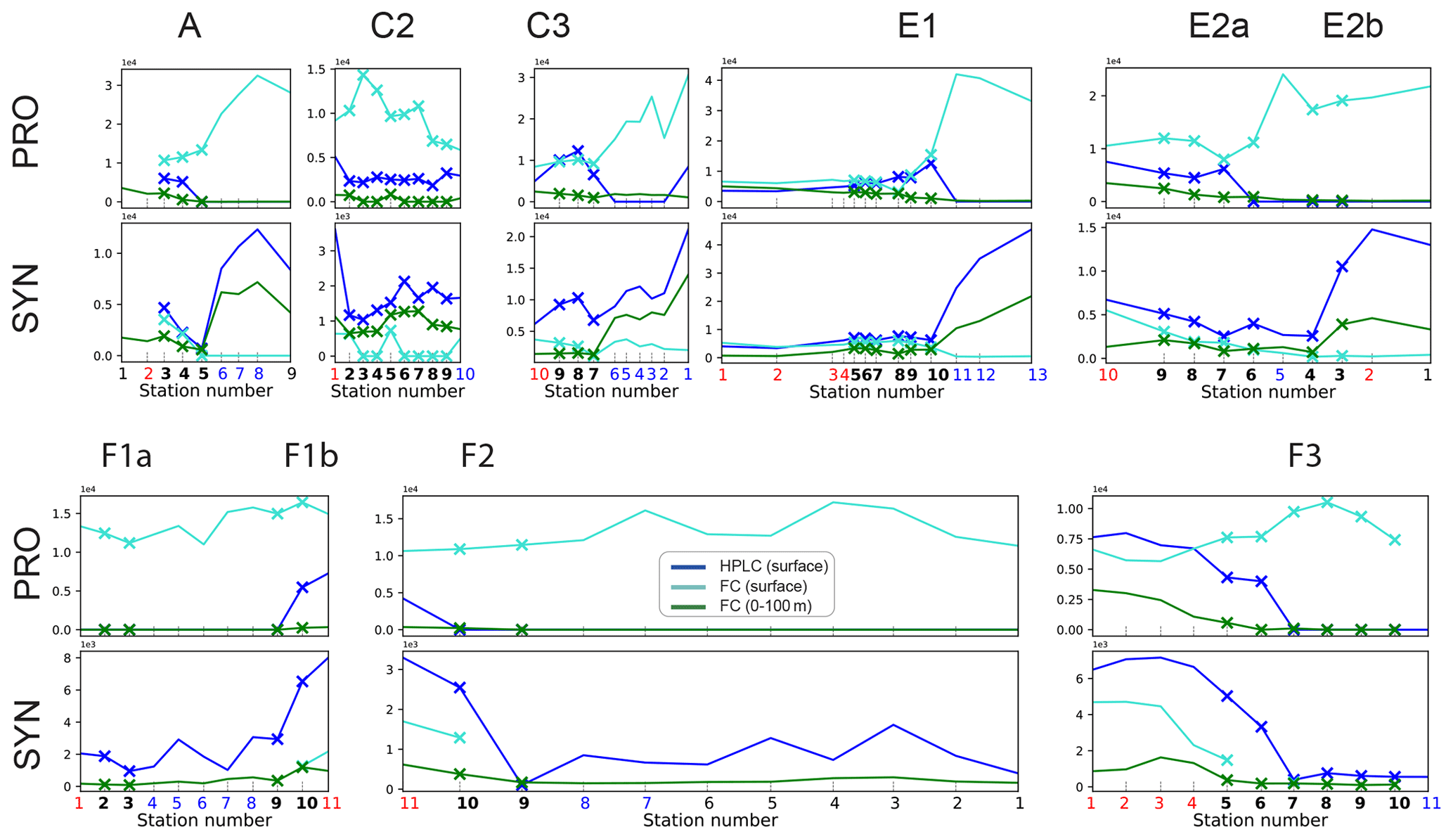
Figure A7Depth-integrated and surface biomass (µg m−3) of cyanobacteria (top row: Prochlorococcus; bottom row: Synechococcus), measured by HPLC and flow cytometry (FC). Front stations are indicated by crosses and the background stations by circles; the numbers of the frontal stations are shown in bold and the warm and cold sides in red and blue.
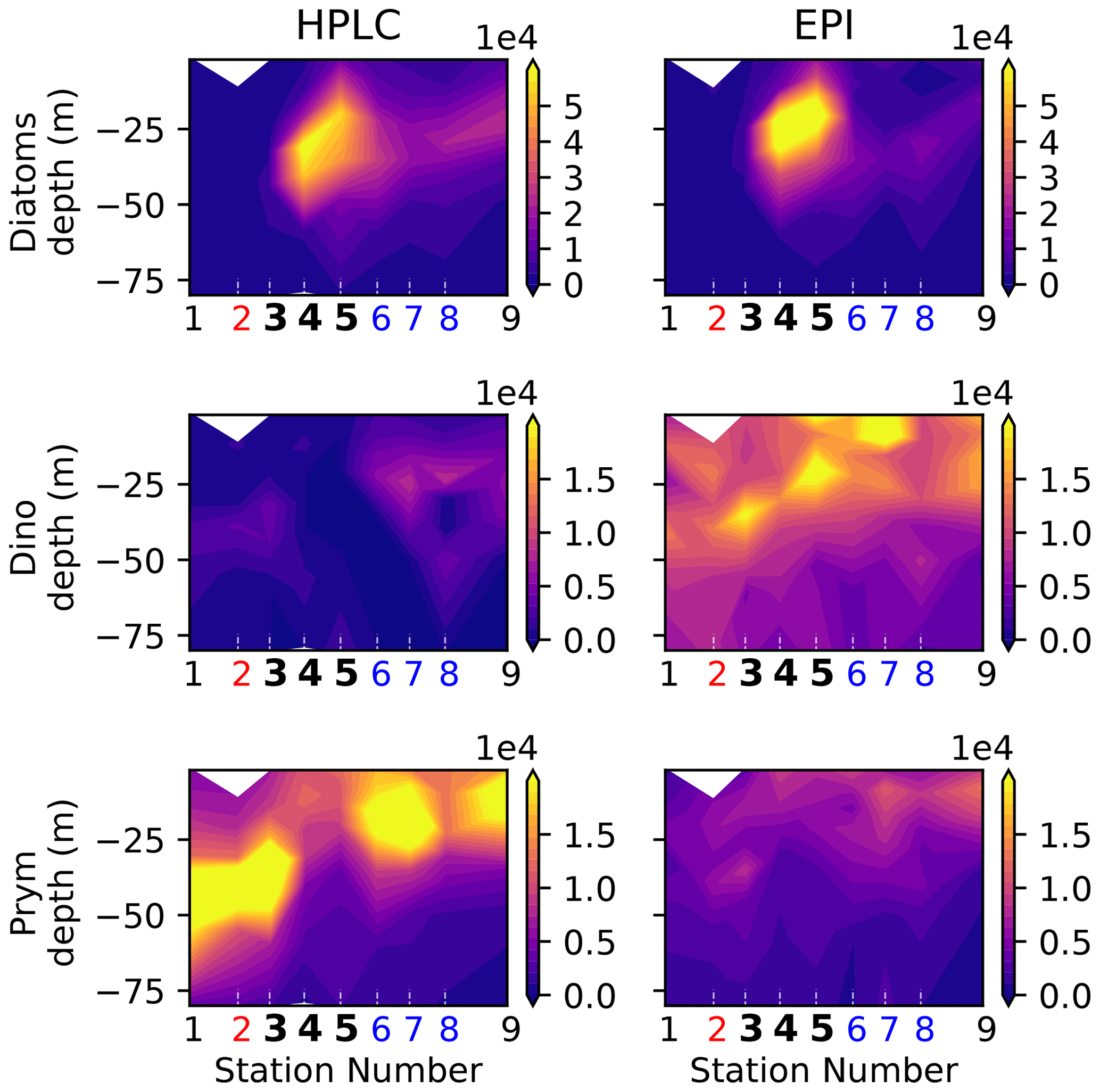
Figure A8Biomass (µgC m−3) of eukaryotic phytoplankton (diatoms, dinoflagellates, and prymnesiophytes) determined by HPLC (this study) and epifluorescence microscopy (see Taylor et al., 2012).
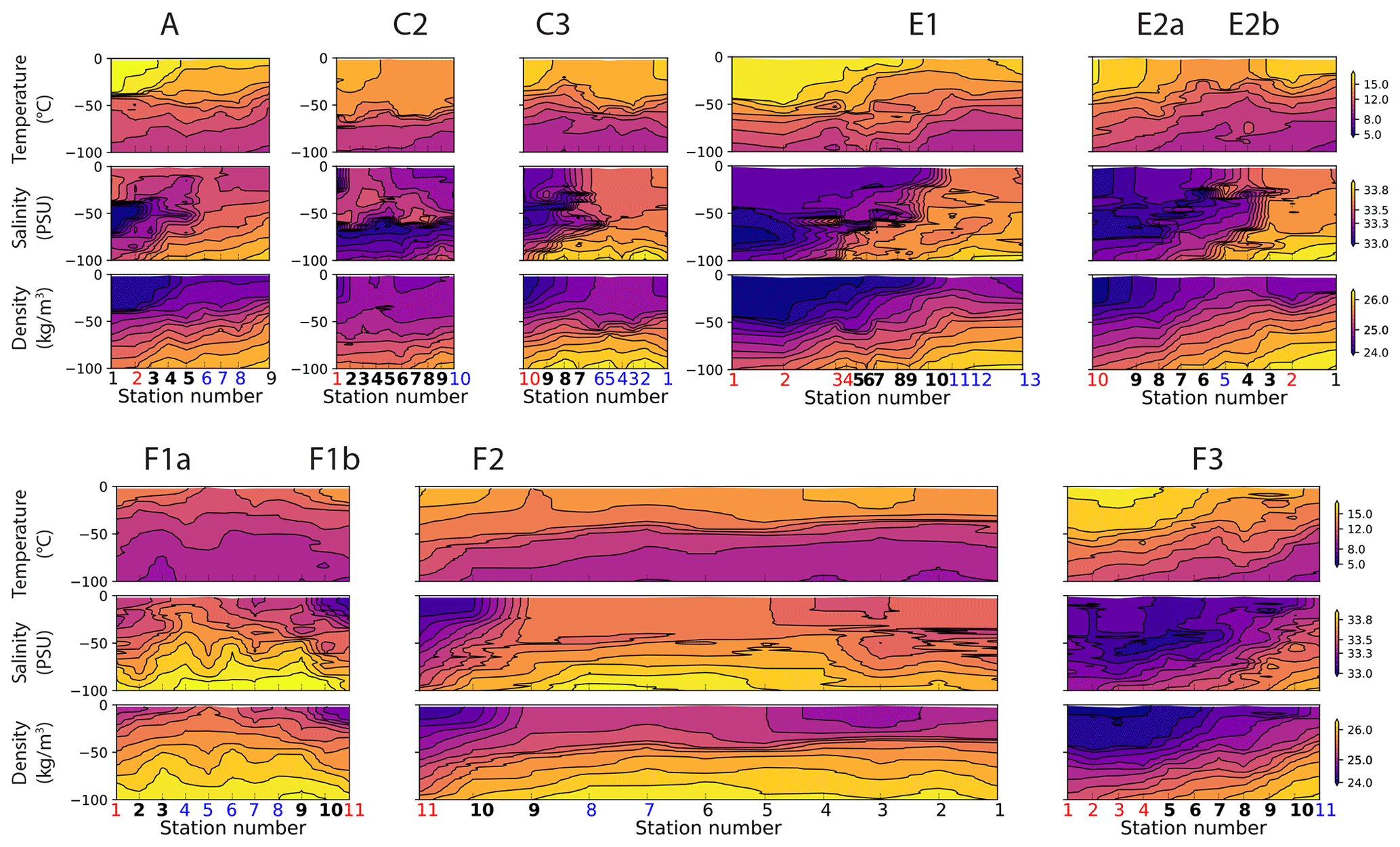
Figure A9Vertical sections of temperature (top row), salinity (middle row), and density (bottom row) in the eight transects. Note that the color scales are identical for all the transects. At the bottom of the plots, the numbers of the frontal stations are shown in bold and the warm and cold sides in red and blue.
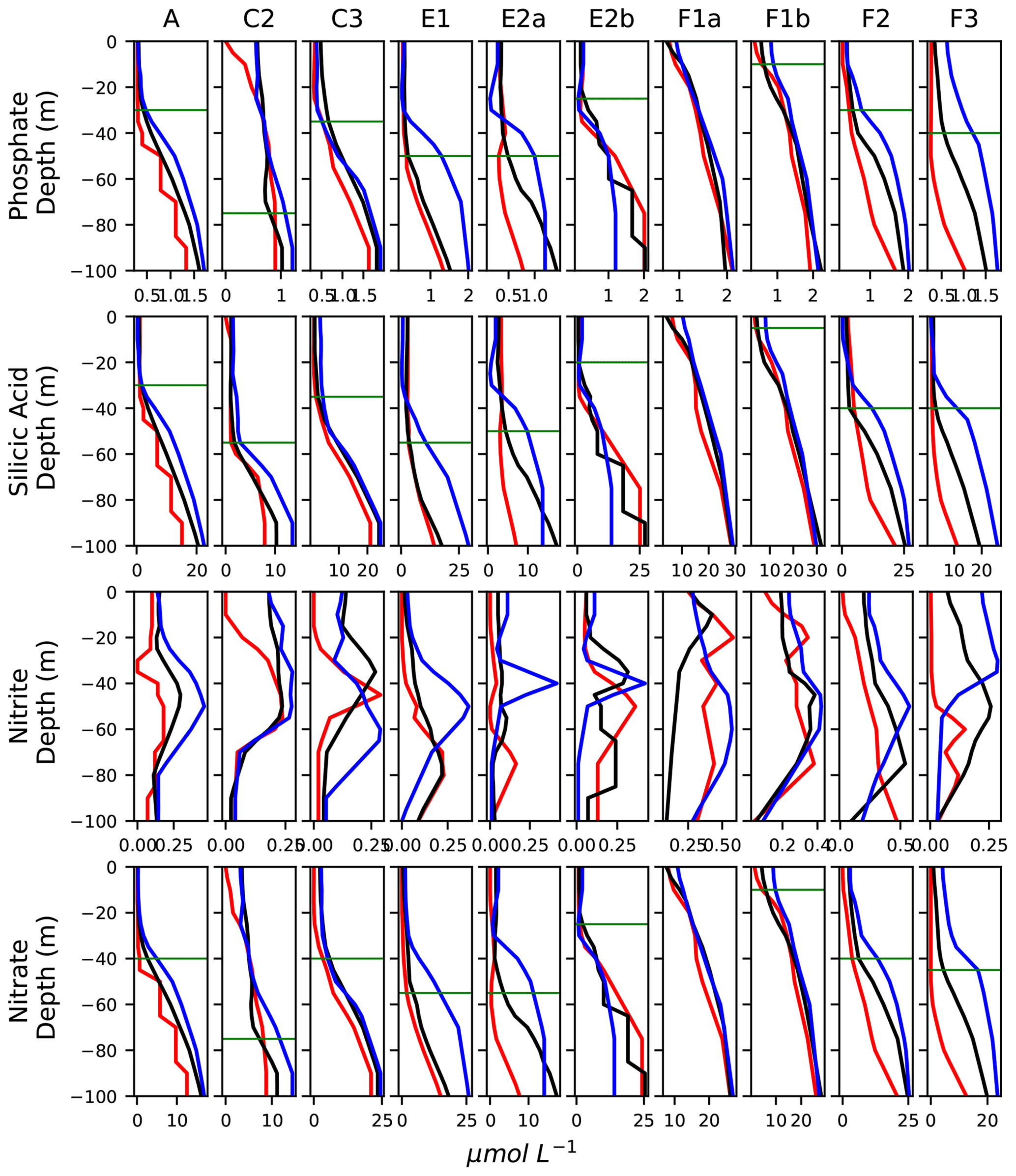
Figure A10Vertical profiles of the concentration of nutrients (in µmol L−1), averaged in the frontal stations (black lines) and the warm and cold background stations (red and blue lines, respectively). The horizontal bars show the depth of the nutricline in the fronts.
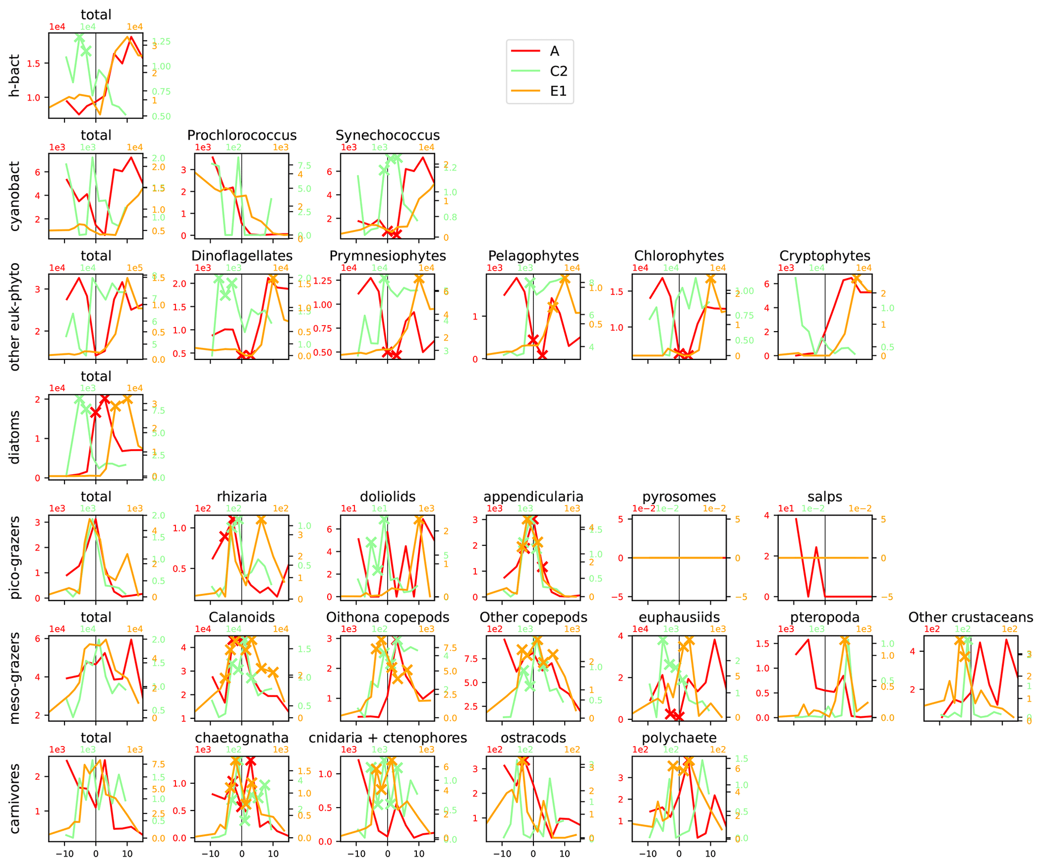
Figure A11Distribution across fronts A, C2, and E1 of the total biomass (µgC m−3) of each trophic group (left column) and biomass of the individual taxa constituting it. The data are centered on the physical density gradient (vertical black lines). The crosses indicate the stations with a biomass peak. The x axis is in kilometers, with 0 at the center of the front.
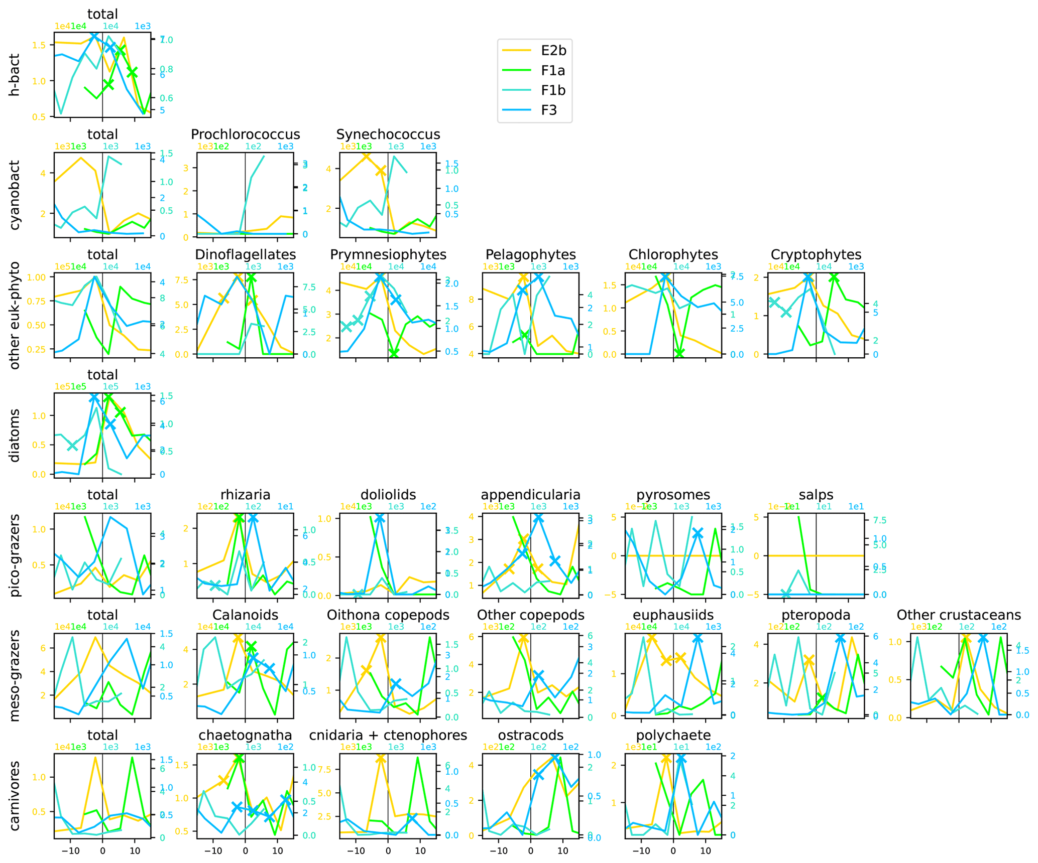
Figure A12Distribution across fronts E2b, F1a, F1b, and F3 of the total biomass (µgC m−3) of each trophic group (left column) and biomass of the individual taxa constituting it. The data are centered on the physical density gradient (vertical black lines). The crosses indicate the stations with a biomass peak. The x axis is in kilometers, with 0 at the center of the front.
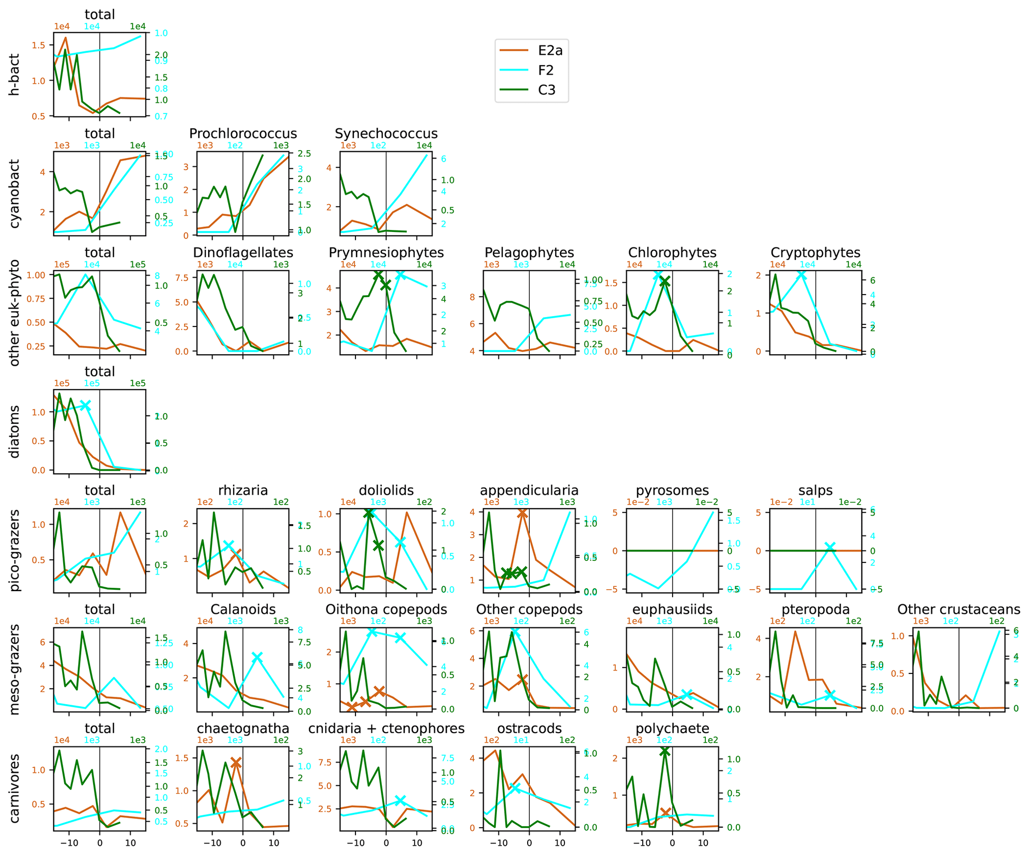
Figure A13Distribution across fronts E2a, F2, and C3 of the total biomass (µgC m−3) of each trophic group (left column) and biomass of the individual taxa constituting it. The data are centered on the physical density gradient (vertical black lines). The crosses indicate the stations with a biomass peak. The x axis is in kilometers, with 0 at the center of the front.
The original datasets are available on the CCE-LTER database (https://oceaninformatics.ucsd.edu/datazoo/catalogs/ccelter/datasets, last access: 8 August 2023) and at the Environmental Data Initiative site (https://edirepository.org/, last access: 8 August 2023):
-
CTD data (https://doi.org/10.6073/pasta/cbc9364bf0868288ab3a4250642cffee, California Current Ecosystem LTER and Goericke, 2017);
-
nutrient data (https://doi.org/10.6073/pasta/0e9975846c4bacf6deae5a3f53c6f9e1, California Current Ecosystem LTER and Goericke, 2022);
-
flow cytometry data (https://doi.org/10.6073/pasta/4d6638460b8a3e8c5ccb95cde821b3ae, California Current Ecosystem LTER and Landry, 2019a);
-
epifluorescence data (https://doi.org/10.6073/pasta/430bc600ff16ec4853fc4d594465e1fe, California Current Ecosystem LTER and Landry, 2019b);
-
HPLC data (https://doi.org/10.6073/pasta/831e099fb086954d3d73638d33d3dd05, California Current Ecosystem LTER and Goericke, 2019, original pigment data).
The code used to perform the analysis, the processed HPLC and ZooScan data, and data files in netCDF format are available at https://doi.org/10.5281/zenodo.7734963 (Mangolte, 2023a).
MDO provided the data. IM conducted the analysis and wrote the manuscript. All authors participated in the discussion and interpretation of the results and reviewed the manuscript.
The contact author has declared that none of the authors has any competing interests.
Publisher’s note: Copernicus Publications remains neutral with regard to jurisdictional claims in published maps and institutional affiliations.
We thank the crews of the ships of the P0810, P1107, P1208, and P1706 CCE-LTER Process cruises, as well as Ralph Goericke, Mike Landry, and the Ohman lab for collecting and processing the samples and providing data. We thank Francesco d'Ovidio, Andrea Doglioli, Pierre Chabert, Peter Franks, and Shailja Gangrade for interesting discussions that helped refine the results.
Inès Mangolte received a PhD scholarship from the École Normale Supérieure and a visiting student Fulbright scholarship, which enabled a 6-month stay at Scripps Institution of Oceanography. The project was supported by funding from CNES. Data collection was supported by the US National Science Foundation (grant nos. OCE-OCE-1026607 and OCE-1637632) for the California Current Ecosystem LTER site.
This paper was edited by Emilio Marañón and reviewed by two anonymous referees.
Allen, J. T., Brown, L., Sanders, R., Moore, C. M., Mustard, A., Fielding, S., Lucas, M., Rixen, M., Savidge, G., Henson, S., and Mayor, D.: Diatom carbon export enhanced by silicate upwelling in the northeast Atlantic, Nature, 437, 728–732, https://doi.org/10.1038/nature03948, 2005. a, b
Ashjian, C. J., Davis, C. S., Gallager, S. M., and Alatalo, P.: Distribution of plankton, particles, and hydrographic features across Georges Bank described using the Video Plankton Recorder, Deep-Sea Res. Pt. II, 48, 245–282, https://doi.org/10.1016/S0967-0645(00)00121-1, 2001. a, b
Barrillon, S., Fuchs, R., Petrenko, A. A., Comby, C., Bosse, A., Yohia, C., Fuda, J.-L., Bhairy, N., Cyr, F., Doglioli, A. M., Grégori, G., Tzortzis, R., d'Ovidio, F., and Thyssen, M.: Phytoplankton reaction to an intense storm in the north-western Mediterranean Sea, Biogeosciences, 20, 141–161, https://doi.org/10.5194/bg-20-141-2023, 2023. a
Barth, J. A., Pierce, S. D., and Smith, R. L.: A separating coastal upwelling jet at Cape Blanco, Oregon and its connection to the California Current System, Deep-Sea Res. Pt. II, 47, 783–810, https://doi.org/10.1016/S0967-0645(99)00127-7, 2000. a
Bednaršek, N. and Ohman, M. D.: Changes in pteropod distributions and shell dissolution across a frontal system in the California Current System, Mar. Ecol.-Prog. Ser., 523, 93–103, https://doi.org/10.3354/meps11199, 2015. a, b
Belkin, I. M.: Review remote sensing of ocean fronts in marine ecology and fisheries, Remote Sens., 13, 1–22, https://doi.org/10.3390/rs13050883, 2021. a
Belkin, I. M. and Helber, R. W.: Physical oceanography of fronts: An editorial, Deep-Sea Res. Pt. II, 119, 1–2, https://doi.org/10.1016/j.dsr2.2015.08.004, 2015. a
Boucher, J.: Localization of zooplankton populations in the Ligurian marine front: role of ontogenic migration, Deep-Sea Res. Pt. A, 31, 469–484, https://doi.org/10.1016/0198-0149(84)90097-9, 1984. a
Bouquet, J. M., Troedsson, C., Novac, A., Reeve, M., Lechtenbörger, A. K., Massart, W., Skaar, K. S., Aasjord, A., Dupont, S., and Thompson, E. M.: Increased fitness of a key appendicularian zooplankton species under warmer, acidified seawater conditions, PLoS One, 13, 1–19, https://doi.org/10.1371/journal.pone.0190625, 2018. a
Brzezinski, M. A., Krause, J. W., Bundy, R. M., Barbeau, K. A., Franks, P., Goericke, R., Landry, M. R., and Stukel, M. R.: Enhanced silica ballasting from iron stress sustains carbon export in a frontal zone within the California Current, J. Geophys. Res.-Oceans, 120, 4654–4669, https://doi.org/10.1002/2015JC010829, 2015. a, b
California Current Ecosystem LTER and Goericke, R.: Conductivity Temperature Depth (CTD) sensor profile data binned by depth from stations within the CCE region from CCE LTER process cruises, 2006–2017 (ongoing), ver. 5, Environmental Data Initiative [data set], https://doi.org/10.6073/pasta/cbc9364bf0868288ab3a4250642cffee, 2017. a, b
California Current Ecosystem LTER and Goericke, R.: High Performance Liquid Chromatography (HPLC) pigment analysis from rosette bottle samples at various depths from CCE LTER process cruises in the California Current System, 2006 to 2017, ver. 4, Environmental Data Initiative [data set], https://doi.org/10.6073/pasta/831e099fb086954d3d73638d33d3dd05, 2019. a, b
California Current Ecosystem LTER and Goericke, R.: Dissolved inorganic nutrients from CCE LTER process cruises, including 5 macro nutrients from water column bottle sample, 2006–2019 (ongoing), ver. 7, Environmental Data Initiative [data set], https://doi.org/10.6073/pasta/0e9975846c4bacf6deae5a3f53c6f9e1, 2022. a, b
California Current Ecosystem LTER and Landry, M.: Picophytoplankton and bacteria total carbon estimates from cell counts analyzed with flow cytometry (FCM) from CCE LTER process cruises in the California Current region, 2006–2017, ver. 4, Environmental Data Initiative [data set], https://doi.org/10.6073/pasta/4d6638460b8a3e8c5ccb95cde821b3ae, 2019a. a, b
California Current Ecosystem LTER and Landry, M.: Size group (pico, nano, micro) and group total carbon estimates from cell counts via epifluorescent microscopy (EPI) of heterotrophic and autotrophic plankton from CCE LTER process cruises in the California Current region, 2006–2016, ver. 4, Environmental Data Initiative [data set], https://doi.org/10.6073/pasta/430bc600ff16ec4853fc4d594465e1fe 2019b. a, b
Capitanio, F. L. and Esnal, G. B.: Vertical distribution of maturity stages of Oikopleura dioica (tunicata, appendicularia) in the frontal system off Valdes Peninsula, Argentina, B. Mar. Sci., 63, 531–539, 1998. a, b
Carreto, J. I., Montoya, N. G., Carignan, M. O., Akselman, R., Acha, E. M., and Derisio, C.: Environmental and biological factors controlling the spring phytoplankton bloom at the Patagonian shelf-break front – Degraded fucoxanthin pigments and the importance of microzooplankton grazing, Prog. Oceanogr., 146, 1–21, https://doi.org/10.1016/j.pocean.2016.05.002, 2016. a
Chabert, P., D'Ovidio, F., Echevin, V., Stukel, M. R., and Ohman, M. D.: Cross-Shore Flow and Implications for Carbon Export in the California Current Ecosystem: A Lagrangian Analysis, J. Geophys. Res.-Oceans, 126, 1–14, https://doi.org/10.1029/2020JC016611, 2021. a, b, c
Chekalyuk, A. M., Landry, M. R., Goericke, R., Taylor, A. G., and Hafez, M. A.: Laser fluorescence analysis of phytoplankton across a frontal zone in the California Current ecosystem, J. Plankton Res., 34, 761–777, https://doi.org/10.1093/plankt/fbs034, 2012. a
Chelton, D. B., Gaube, P., Schlax, M. G., Early, J. J., and Samelson, R. M.: The influence of nonlinear mesoscale eddies on near-surface oceanic chlorophyll, Science, 334, 328–332, https://doi.org/10.1126/science.1208897, 2011. a
Claustre, H., Kerherve, P., Marty, J. C., Prieur, L., Videau, C., and Hecq, J. H.: Phytoplankton dynamics associated with a geostrophic front: Ecological and biogeochemical implications, J. Mar. Res., 52, 711–742, https://doi.org/10.1357/0022240943077000, 1994. a
Clayton, S., Dutkiewicz, S., Jahn, O., and Follows, M. J.: Dispersal, eddies, and the diversity of marine phytoplankton, Limnol. Oceanogr. Fluids Environ., 3, 182–197, https://doi.org/10.1215/21573689-2373515, 2013. a
Clayton, S., Nagai, T., and Follows, M. J.: Fine scale phytoplankton community structure across the Kuroshio Front, J. Plankton Res., 36, 1017–1030, https://doi.org/10.1093/plankt/fbu020, 2014. a
Clayton, S., Lin, Y. C., Follows, M. J., and Worden, A. Z.: Co-existence of distinct Ostreococcus ecotypes at an oceanic front, Limnol. Oceanogr., 62, 75–88, https://doi.org/10.1002/lno.10373, 2017. a
De Verneil, A. and Franks, P. J.: A pseudo-Lagrangian method for remapping ocean biogeochemical tracer data: Calculation of net Chl-a growth rates, J. Geophys. Res.-Oceans, 120, 4962–4979, https://doi.org/10.1002/2015JC010898, 2015. a
de Verneil, A., Franks, P. J., and Ohman, M. D.: Frontogenesis and the Creation of Fine-Scale Vertical Phytoplankton Structure, J. Geophys. Res.-Oceans, 124, 1509–1523, https://doi.org/10.1029/2018JC014645, 2019. a, b, c, d, e, f, g
Derisio, C., Alemany, D., Acha, E. M., and Mianzan, H.: Influence of a tidal front on zooplankton abundance, assemblages and life histories in Península Valdés, Argentina, J. Marine Syst., 139, 475–482, https://doi.org/10.1016/j.jmarsys.2014.08.019, 2014. a, b
D'Ovidio, F., Fernández, V., Hernández-García, E., and López, C.: Mixing structures in the Mediterranean Sea from finite-size Lyapunov exponents, Geophys. Res. Lett., 31, 1–4, https://doi.org/10.1029/2004GL020328, 2004. a
Eiane, K. and Ohman, M. D.: Stage-specific mortality of Calanus finmarchicus, Pseudocalanus elongatus and Oithona similis on Fladen Ground, North Sea, during a spring bloom, Mar. Ecol.-Prog. Ser., 268, 183–193, https://doi.org/10.3354/meps268183, 2004. a
Fifani, G., Baudena, A., Fakhri, M., Baaklini, G., Faugère, Y., Morrow, R., Mortier, L., and D'ovidio, F.: Drifting speed of lagrangian fronts and oil spill dispersal at the ocean surface, Remote Sens., 13, 1–26, https://doi.org/10.3390/rs13224499, 2021. a
Franks, P. J.: Sink or swim: Accumulation of biomass at fronts, Mar. Ecol.- Prog. Ser., 82, 1–12, https://doi.org/10.3354/meps082001, 1992. a
Gangrade, S. and Franks, P. J.: Phytoplankton patches at oceanic fronts are linked to coastal upwelling pulses: Observations and implications in the California Current System, J. Geophys. Res.-Oceans, 128, e2022JC019095, https://doi.org/10.1029/2022JC019095, 2023. a, b, c
Garrison, D. L., Gowing, M. M., Hughes, M. P., Campbell, L., Caron, D. A., Dennett, M. R., Shalapyonok, A., Olson, R. J., Landry, M. R., Brown, S. L., Liu, H. B., Azam, F., Steward, G. F., Ducklow, H. W., and Smith, D. C.: Microbial food web structure in the Arabian Sea: A US JGOFS study, Deep-Sea Res. Pt. II, 47, 1387–1422, https://doi.org/10.1016/S0967-0645(99)00148-4, 2000. a
Goericke, R.: The structure of marine phytoplankton communities- patterns, rules and mechanisms, Calif. Coop. Ocean. Fish. Investig. Reports, 52, 182–197, 2011. a
Goericke, R. and Montoya, J. P.: Estimating the contribution of microalgal taxa to chlorophyll a in the field – Variations of pigment ratios under nutrient- and light-limited growth, Mar. Ecol.-Prog. Ser., 169, 97–112, https://doi.org/10.3354/meps169097, 1998. a
Gorsky, G., Ohman, M. D., Picheral, M., Gasparini, S., Stemmann, L., Romagnan, J. B., Cawood, A., Pesant, S., García-Comas, C., and Prejger, F.: Digital zooplankton image analysis using the ZooScan integrated system, J. Plankton Res., 32, 285–303, https://doi.org/10.1093/plankt/fbp124, 2010. a
Graham, W. M., Pagès, F., and Hamner, W. M.: A physical context for gelatinous zooplankton aggregations: A review, Hydrobiologia, 451, 199–212, https://doi.org/10.1023/A:1011876004427, 2001. a, b
Haberlin, D., Raine, R., McAllen, R., and Doyle, T. K.: Distinct gelatinous zooplankton communities across a dynamic shelf sea, Limnol. Oceanogr., 64, 1802–1818, https://doi.org/10.1002/lno.11152, 2019. a
Haëck, C., Lévy, M., Mangolte, I., and Bopp, L.: Satellite data reveal earlier and stronger phytoplankton blooms over fronts in the Gulf Stream region, Biogeosciences, 20, 1741–1758, https://doi.org/10.5194/bg-20-1741-2023, 2023. a
Hoskins, B. J.: The mathematical theory of frontogenesis, Annu. Rev. Fluid Mech., 14, 131–151, 1982. a
Klein, P. and Lapeyre, G.: The oceanic vertical pump induced by mesoscale and submesoscale turbulence, Annu. Rev. Mar. Sci., 1, 351–375, https://doi.org/10.1146/annurev.marine.010908.163704, 2009. a, b
Kosro, P. M. and Huyer, A.: CTD and velocity surveys of seaward jets off northern California, July 1981 and 1982, J. Geophys. Res., 91, 7680, https://doi.org/10.1029/jc091ic06p07680, 1986. a
Kotori, M.: Life cycle and growth rate of the chaetognath parasagitta elegans in the northern North Pacific Ocean, Plankt. Biol. Ecol., 46, 153–158, 1999. a
Krause, J. W., Brzezinski, M. A., Goericke, R., Landry, M. R., Ohman, M. D., Stukel, M. R., and Taylor, A. G.: Variability in diatom contributions to biomass, organic matter production and export across a frontal gradient in the California Current Ecosystem, J. Geophys. Res.-Oceans, 120, 1032–1047, https://doi.org/10.1002/2014JC010472, 2015. a, b
Landry, M. R., Ohman, M. D., Goericke, R., Stukel, M. R., Barbeau, K. A., Bundy, R., and Kahru, M.: Pelagic community responses to a deep-water front in the California Current Ecosystem: Overview of the A-Front Study, J. Plankton Res., 34, 739–748, https://doi.org/10.1093/plankt/fbs025, 2012. a, b
Lavaniegos, B. E. and Ohman, M. D.: Coherence of long-term variations of zooplankton in two sectors of the California Current System, Prog. Oceanogr., 75, 42–69, https://doi.org/10.1016/j.pocean.2007.07.002, 2007. a
Lévy, M., Ferrari, R., Franks, P. J., Martin, A. P., and Rivière, P.: Bringing physics to life at the submesoscale, Geophys. Res. Lett., 39, L14602, https://doi.org/10.1029/2012GL052756, 2012. a
Lévy, M., Jahn, O., Dutkiewicz, S., and Follows, M. J.: Phytoplankton diversity and community structure affected by oceanic dispersal and mesoscale turbulence, Limnol. Oceanogr. Fluids Environ., 4, 67–84, https://doi.org/10.1215/21573689-2768549, 2014. a, b
Lévy, M., Jahn, O., Dutkiewicz, S., Follows, M. J., and D'Ovidio, F.: The dynamical landscape of marine phytoplankton diversity, J. R. Soc. Interface, 12, 20150481, https://doi.org/10.1098/rsif.2015.0481, 2015. a, b
Lévy, M., Franks, P. J., and Smith, K. S.: The role of submesoscale currents in structuring marine ecosystems, Nat. Commun., 9, 4758, https://doi.org/10.1038/s41467-018-07059-3, 2018. a
Lewandowska, A. M., Striebel, M., Feudel, U., Hillebrand, H., and Sommer, U.: The importance of phytoplankton trait variability in spring bloom formation, ICES J. Mar. Sci., 72, 1908–1915, https://doi.org/10.1093/icesjms/fsv059, 2015. a
Li, Q. P., Franks, P. J., Landry, M. R., Goericke, R., and Taylor, A. G.: Modeling phytoplankton growth rates and chlorophyll to carbon ratios in California coastal and pelagic ecosystems, J. Geophys. Res.-Biogeo., 115, 1–12, https://doi.org/10.1029/2009JG001111, 2010. a
Li, Q. P., Franks, P. J., Ohman, M. D., and Landry, M. R.: Enhanced nitrate fluxes and biological processes at a frontal zone in the southern California current system, J. Plankton Res., 34, 790–801, https://doi.org/10.1093/plankt/fbs006, 2012. a
Liu, X. and Levine, N. M.: Enhancement of phytoplankton chlorophyll by submesoscale frontal dynamics in the North Pacific Subtropical Gyre, Geophys. Res. Lett., 43, 1651–1659, https://doi.org/10.1002/2015GL066996, 2016. a
Lohrenz, S. E., Cullen, J. J., Phinney, D. A., Olson, D. B., and Yentsch, C. S.: Distributions of pigments and primary production in a Gulf Stream meander, J. Geophys. Res., 98, 14545–14560, https://doi.org/10.1029/93jc00678, 1993. a
Luo, J. Y., Grassian, B., Tang, D., Irisson, J. O., Greer, A. T., Guigand, C. M., McClatchie, S., and Cowen, R. K.: Environmental drivers of the fine-scale distribution of a gelatinous zooplankton community across a mesoscale front, Mar. Ecol.-Prog. Ser., 510, 129–149, https://doi.org/10.3354/meps10908, 2014. a, b
Mahadevan, A.: The Impact of Submesoscale Physics on Primary Productivity of Plankton, Annu. Rev. Mar. Sci., 8, 161–184, https://doi.org/10.1146/annurev-marine-010814-015912, 2016. a
Mangolte, I.: CCE fronts, Zenodo [code, data set], https://doi.org/10.5281/zenodo.7734963, 2023a. a, b
Mangolte, I.: CCE-fronts A, TIB [video], https://doi.org/10.5446/61004, 2023b. a, b, c, d, e
Mangolte, I.: CCE-fronts C, TIB [video], https://doi.org/10.5446/61005, 2023c. a, b, c, d, e
Mangolte, I.: CCE-fronts E, TIB [video], https://doi.org/10.5446/61006, 2023d. a, b, c, d, e, f
Mangolte, I.: CCE-fronts F, TIB [video], https://doi.org/10.5446/61007, 2023e. a, b, c, d, e
Mangolte, I., Lévy, M., Dutkiewicz, S., Clayton, S., and Jahn, O.: Plankton community response to fronts: winners and losers, J. Plankton Res., 44, 241–258, https://doi.org/10.1093/plankt/fbac010, 2022. a, b
Mauzole, Y. L., Torres, H. S., and Fu, L. L.: Patterns and Dynamics of SST Fronts in the California Current System, J. Geophys. Res.-Oceans, 125, e2019JC015499, https://doi.org/10.1029/2019JC015499, 2020. a, b
Mousing, E. A., Richardson, K., Bendtsen, J., Cetinić, I., and Perry, M. J.: Evidence of small-scale spatial structuring of phytoplankton alpha- and beta-diversity in the open ocean, J. Ecol., 104, 1682–1695, https://doi.org/10.1111/1365-2745.12634, 2016. a
Oguz, T., Macias, D., and Tintore, J.: Ageostrophic frontal processes controlling phytoplankton production in the Catalano-Balearic Sea (Western Mediterranean), PLoS One, 10, e0129045, https://doi.org/10.1371/journal.pone.0129045, 2015. a
Ohman, M. D., Powell, J. R., Picheral, M., and Jensen, D. W.: Mesozooplankton and particulate matter responses to a deep-water frontal system in the southern California Current System, J. Plankton Res., 34, 815–827, https://doi.org/10.1093/plankt/fbs028, 2012. a, b, c, d
Ohman, M. D., Barbeau, K., Franks, P. J., Goericke, R., Landry, M. R., and Miller, A. J.: Ecological transitions in a coastal upwelling ecosystem, Oceanography, 26, 210–219, https://doi.org/10.5670/oceanog.2013.65, 2013. a
Pollard, R. T. and Regier, L. A.: Vorticity and vertical circulation at an ocean front, J. Phys. Oceanogr., 22, 609–625, https://doi.org/10.1175/1520-0485(1992)022<0609:VAVCAA>2.0.CO;2, 1992. a
Powell, J. R. and Ohman, M. D.: Changes in zooplankton habitat, behavior, and acoustic scattering characteristics across glider-resolved fronts in the Southern California Current System, Prog. Oceanogr., 134, 77–92, https://doi.org/10.1016/j.pocean.2014.12.011, 2015. a, b
Prants, S. V.: Marine life at Lagrangian fronts, Prog. Oceanogr., 204, 102790, https://doi.org/10.1016/j.pocean.2022.102790, 2022. a
Renault, L., McWilliams, J. C., Kessouri, F., Jousse, A., Frenzel, H., Chen, R., and Deutsch, C.: Evaluation of high-resolution atmospheric and oceanic simulations of the California Current System, Prog. Oceanogr., 195, 102564, https://doi.org/10.1016/j.pocean.2021.102564, 2021. a
Ribalet, F., Marchetti, A., Hubbard, K. A., Brown, K., Durkin, C. A., Morales, R., Robert, M., Swalwell, J. E., Tortell, P. D., and Armbrust, E. V.: Unveiling a phytoplankton hotspot at a narrow boundary between coastal and offshore waters, P. Natl. Acad. Sci. USA, 107, 16571–16576, https://doi.org/10.1073/pnas.1005638107, 2010. a, b
Rousselet, L., de Verneil, A., Doglioli, A. M., Petrenko, A. A., Duhamel, S., Maes, C., and Blanke, B.: Large- to submesoscale surface circulation and its implications on biogeochemical/biological horizontal distributions during the OUTPACE cruise (southwest Pacific), Biogeosciences, 15, 2411–2431, https://doi.org/10.5194/bg-15-2411-2018, 2018. a
Samo, T. J., Pedler, B. E., Ball, G. I., Pasulka, A. L., Taylor, A. G., Aluwihare, L. I., Azam, F., Goericke, R., and Landry, M. R.: Microbial distribution and activity across a water mass frontal zone in the California Current Ecosystem, J. Plankton Res., 34, 802–814, https://doi.org/10.1093/plankt/fbs048, 2012. a
Stukel, M. R., Aluwihare, L. I., Barbeau, K. A., Chekalyuk, A. M., Goericke, R., Miller, A. J., Ohman, M. D., Ruacho, A., Song, H., Stephens, B. M., and Landry, M. R.: Mesoscale ocean fronts enhance carbon export due to gravitational sinking and subduction, P. Natl. Acad. Sci. USA, 114, 1252–1257, https://doi.org/10.1073/pnas.1609435114, 2017. a, b
Taylor, A. G. and Landry, M. R.: Phytoplankton biomass and size structure across trophic gradients in the southern California Current and adjacent ocean ecosystems, Mar. Ecol.-Prog. Ser., 592, 1–17, https://doi.org/10.3354/meps12526, 2018. a
Taylor, A. G., Goericke, R., Landry, M. R., Selph, K. E., Wick, D. A., and Roadman, M. J.: Sharp gradients in phytoplankton community structure across a frontal zone in the California Current Ecosystem, J. Plankton Res., 34, 778–789, https://doi.org/10.1093/plankt/fbs036, 2012. a, b, c
Thibault, D., Gaudy, R., and Le Fèvre, J.: Zooplankton biomass, feeding and metabolism in a geostrophic frontal area (Almeria-Oran Front, western Mediterranean). Significance to pelagic food webs, J. Marine Syst., 5, 297–311, https://doi.org/10.1016/0924-7963(94)90052-3, 1994. a, b
Tzortzis, R., Doglioli, A. M., Barrillon, S., Petrenko, A. A., d'Ovidio, F., Izard, L., Thyssen, M., Pascual, A., Barceló-Llull, B., Cyr, F., Tedetti, M., Bhairy, N., Garreau, P., Dumas, F., and Gregori, G.: Impact of moderately energetic fine-scale dynamics on the phytoplankton community structure in the western Mediterranean Sea, Biogeosciences, 18, 6455–6477, https://doi.org/10.5194/bg-18-6455-2021, 2021. a, b, c
Yoder, J. A., Ackleson, S. G., Barber, R. T., Flament, P., and Balch, W. M.: A line in the sea, Nature, 371, 689–692, https://doi.org/10.1038/371689a0, 1994. a
Zaba, K. D., Franks, P. J., and Ohman, M. D.: The California Undercurrent as a Source of Upwelled Waters in a Coastal Filament, J. Geophys. Res.-Oceans, 126, e2020JC016602, https://doi.org/10.1029/2020JC016602, 2021. a, b, c