The bottom mixed layer depth as an indicator of subsurface Chlorophyll a distribution

Primary production dynamics are strongly associated with vertical density profiles in shelf waters. Variations in the vertical structure of the pycnocline in stratified shelf waters are likely to affect nutrient fluxes and hence the vertical distribution and production rate of phytoplankton. To understand the effects of physical changes on primary production, identifying the linkage between water column density and Chlorophyll a (Chl a) profiles is essential. Here, the vertical distributions of density features describing three different portions of the pycnocline (the top, centre, and bottom) were compared to the vertical distribution of Chl a to provide auxiliary variables to estimate Chl a in shelf waters. The proximity of density features with deep Chl a maximum (DCM) was tested using the Spearman correlation, linear regression, and a major axis regression over 15 years in a shelf sea region (the northern North Sea) that exhibits stratified water columns. Out of 1237 observations, 78 % reported DCM above the bottom mixed layer depth (BMLD: depth between the bottom of the pycnocline and the mixed layer underneath) with an average distance of 2.74 ± 5.21 m from each other. BMLD acts as a vertical boundary above which subsurface Chl a maxima are mostly found in shelf seas (depth ≤ 115 m). Overall, DCMs were correlated with the halfway pycnocline depth (HPD) (ρ_S = 0.56) which, combined with BMLD, were better predictors of the locations of DCMs than surface mixed layer indicators and the maximum squared buoyancy frequency. These results suggest a significant contribution of deep mixing processes in defining the vertical distribution of subsurface production in stratified waters and indicate BMLD as a potential indicator of the Chl a spatiotemporal variability in shelf seas. An analytical approach integrating the threshold and the maximum angle method is proposed to extrapolate BMLD, the surface mixed layer, and DCM from in situ vertical samples.

1 Introduction

As we begin to manage our oceans and shelf seas for more complex simultaneous uses, such as renewable energy development, fishing, and marine protected areas, it is becoming increasingly important to understand the details of primary productivity at fine spatial scales. Besides very shallow waters, the vast majority of phytoplankton production in continental shelf waters generally occurs under stratified conditions, where the pycnocline provides a stable habitat for phytoplankton growth in the lower euphotic zone. The seasonal heating–cooling cycle of the water column regulates the stratification in temperate shelf waters, where the intensified solar radiation in spring–summer increases the difference of temperature and salinity between surface and deep waters and prompts the formation of a pycnocline dividing the surface from deep mixed waters. Once the stratification is set in spring–summer, turbulent mixing represents the main source of new nutrients into the pycnocline during prolonged stratified conditions. Climate change (Holt et al., 2016, 2018) and the introduction of numerous man-made infrastructure (e.g. offshore wind farms, Dorrell et al., 2022) are expected to alter the balance between mixing and stratification in shelf regions, affecting the vertical exchange of nutrients between deep and surface waters (below and above the pycnocline). Anomalies such as circulation slowdown, sea-level rise, bottom and surface temperature, wind speed, and wave height have largely been described as a consequence of climate change in the last 2 decades (e.g. Orihuela-Pinto et al., 2022; Taboada and Anadón, 2012; Bonaduce et al., 2019), while the consequences of these physical changes on the biological processes are still only partially understood (Lozier et al., 2011; Somavilla et al., 2017).

1.1 Subsurface Chlorophyll a maxima

Many of the uncertainties related to estimating primary production abundance are related to the difficulties in retrieving correct concentrations throughout the water column. Contrary to the detection of surface blooms by satellite sensors, subsurface Chlorophyll a maxima (SCMs) are often more difficult to measure. SCMs represent significant features in plankton systems (Cullen, 2015), define where most of the bottom-up processes take place, can persist in separate vertical layers, and encompass more than 50 % of overall water column production (Weston et al., 2005; Takahashi and Hori, 1984). In the North Sea, summertime (May–August) subsurface production contributes to 20 %–50 % of the annual production and sustains the food chain in continental shelf waters during prolonged stratified conditions (Hickman et al., 2012; Richardson and Pedersen, 1998; Weston et al., 2005). Several studies have linked the vertical distribution of deep Chlorophyll a maxima (DCMs) to deep mixing processes (e.g. Brown et al., 2015; Richardson and Pedersen, 1998; Sharples et al., 2006) and identified the occurrence of deep assemblages in the proximity of the pycnocline in shelf seas (e.g. Costa et al., 2020; Durán-Campos et al., 2019; Ross and Sharples, 2007; Sharples et al., 2001). DCMs have been identified close to the base of the pycnocline in regions of strong tidal mixing in the Georges Bank in August (Holligan et al., 1984) and in the western English Channel (Sharples et al., 2001). However, despite the clear linkage between SCMs and subsurface physical processes in shelf seas, only surface mixing processes have been used to investigate the global variations of primary production (Somavilla et al., 2017; Steinacher et al., 2010), making the surface mixed layer depth (MLD) one of the main indicator for the variations of density structures and marine primary production. However, shelf ecosystems are equally driven by physical processes occurring above and below the pycnocline (Wihsgott et al., 2019), making the identification of the upper and lower limits of the pycnocline essential to understanding the processes defining the primary production in shelf waters.

1.2 The surface mixed layer depth (MLD)

MLD has been largely considered as a central variable for understanding phytoplankton dynamics (Sverdrup, 1953), especially in oceanic sites, where several studies have investigated the association of MLD with the Chl a vertical distribution (Behrenfeld, 2010; Carranza et al., 2018; Diehl, 2002; Gradone et al., 2020), phytoplankton bloom events (Behrenfeld, 2010; Chiswell, 2011; D'Ortenzio et al., 2014; Prend et al., 2019; Ryan-Keogh and Thomalla, 2020, Sverdrup, 1953), and the effects of climate change (Somavilla et al., 2017). The nutricline depth exhibits positive correlations with the upper mixed layer depth (Ducklow et al., 2007; Gradone et al., 2020; Holligan et al., 1984; Prézelin et al., 2000, 2004; Ryan-Keogh and Thomalla, 2020; Yentsch, 1974, 1980), and it has been generally associated with surface spring blooms or windstorm events (Carranza et al., 2018; Carvalho et al., 2017). However, the effects of MLD and climate variations on primary production are still an unsolved question (Lozier et al., 2011; Somavilla et al., 2017). The need for a much more detailed understanding of the linkage between primary production, pycnocline characteristics, and deep turbulent processes (below the pycnocline) is therefore a key area of research, especially in highly productive but spatially heterogeneous areas such as shelf waters and shallow seas.

The methods for identifying MLDs vary among marine environments, hydrodynamic regimes, and the spatial resolution of vertical profiles (Courtois et al., 2017; Lorbacher et al., 2006) because making use of a single method is difficult for spatiotemporally heterogeneous regions. MLDs are typically defined as the depth at which the density exceeds a specific value (threshold method); however, this method presents issues in specific hydrodynamic conditions, such as over estimating MLD in regions with deep convection (e.g. subpolar oceans; Courtois et al., 2017) or misidentifying water columns as a newly established shallow MLD over previous periods of stratification (Somavilla et al., 2017). Several sensitivity tests and comparisons have been conducted in oceanic waters (González-Pola et al., 2007; Holte and Talley, 2009; Courtois et al., 2017); however, there are no standard methods for MLD identification either in shelf or oceanic waters.

1.3 A new way forward: the bottom mixed layer depth (BMLD) as an indicator of deep Chl a maxima (DCMs) in shelf waters

In temperate shelf waters after spring blooms, phytoplankton adapt to grow at the subsurface under low light and nutrient conditions where new primary production is sustained by upward nutrient fluxes from the mixed layer below the pycnocline (bottom mixed layer, BML; Pingree and Griffiths, 1977; Wihsgott et al., 2019). Several studies reported vertical distributions of SCMs close to the base of the pycnocline (e.g. Costa et al., 2020; Durán-Campos et al., 2019), especially in stratified waters affected by tidal currents in the proximity of shelf banks. As an example, spring tides have been shown to trigger a hydraulic jump on the edge of the Jones Bank (Celtic Sea, UK) that is sufficient to increase the mixing at the base of the pycnocline and inject it with new nutrients (Palmer et al., 2013). The BML is crucial in supporting subsurface primary production in resource limited environments where turbulent mixing in the proximity of the thermocline introduces new nutrients in surface waters and removes phytoplankton from the SCM into deep waters (western English Channel, Sharples et al., 2001). The upward transfer of nutrients and downward fluxes of phytoplankton occurring at the base of the pycnocline suggests this depth is a central location of carbon fluxes in temperate shelf waters (Sharples et al., 2001), making the upper limit of the bottom mixed layer in the proximity of the base of the pycnocline (hereafter called bottom mixed layer depth, BMLD) a key variable for estimating productivity. In the literature, BMLD has been identified as the depth where density changes by −0.02 kg m⁻³ relative to the closest value to the seabed (Sharples et al., 2001; Wihsgott et al., 2019; Poulton et al., 2022; Hopkins et al., 2021) or by 0.01–0.1 ^∘C above the near-bed temperature (Palmer et al., 2013; Pingree and Griffiths, 1977). This study includes the following.

• We propose the adaptation of existing methods (threshold and maximum angle methods from Chu and Fan, 2011) into a new algorithm able to process different vertical distributions of high-resolution (1 m) density profiles (characterized by split pycnoclines) to identify (i) the surface mixed layer (MLD) and (ii) the bottom mixed layer depth (BMLD) in stratified waters.

• Depth-integrated Chl a is compared among the sections above and below stratification features (MLD; halfway pycnocline depth, HPD; BMLD; and maximum squared buoyancy frequency) in shelf waters (20–120 m) using 15 years of repeated surveys covering a mosaic of habitats types: seasonally stratified waters, permanently mixed waters, regions of freshwater inputs, and strong tidal mixing (van Leeuwen et al., 2015). DCMs are hypothesized to be distributed at the same depth of stratification structures to test where summertime subsurface Chl a is distributed more frequently in regard to the pycnocline (e.g. DCMs at the most stratified layer identified by Max N² or at the base of the pycnocline).

• Further scrutiny was applied to BMLD to investigate to what extent it provides information on the vertical distribution of DCMs in temperate, stratified shelf waters during summer, regardless of phytoplankton dynamics (cell light history regulating photoacclimation) or physical conditions of the water column (e.g. stability).

2 Methods

2.1 Oceanographic data

In situ summertime measurements of temperature, salinity, and Chl a were collected by a towed and undulating CTD-fluorometer and by a vertical CTD-fluorometer in the North Sea off the east coast of Scotland, UK, within the Firth of Forth (FoF) and Tay region for over 15 years (from 2000 to 2014; Fig. 1). A total of 1273 profiles from both types of sampling were extracted from April to August (April = 3, May = 51, June = 1115, July = 66, August = 38). There were 426 profiles from the sea surface to the seabed (vertical resolution of 1 decibar) collected at fixed stations from 12 oceanographic campaigns carried out by Marine Scotland Science on board the fisheries research vessels Scotia and Alba na Mara (https://www.gov.scot/marine-and-fisheries/, last access: 19 December 2023). Water samples were collected during each cast for calibration of the in situ sensor data. The undulating CTD-fluorometer sampled the water column in June 2003 and July 2014 with a continuous vertical and horizontal oscillation of the instrument throughout the water column from 2–5 m below the sea surface to 5 m from the seabed. The continuous profiles obtained from the undulating CTD-fluorometer were converted into 847 single profiles of the water columns. Data were sampled at 1 s intervals, resulting in a vertical resolution of between 0.5 and 1 m in water depths of 25 to 115 m. Further information about the oceanographic cruise in June 2003 is described by Scott et al. (2010), whose method was applied in the cruise in July 2014.

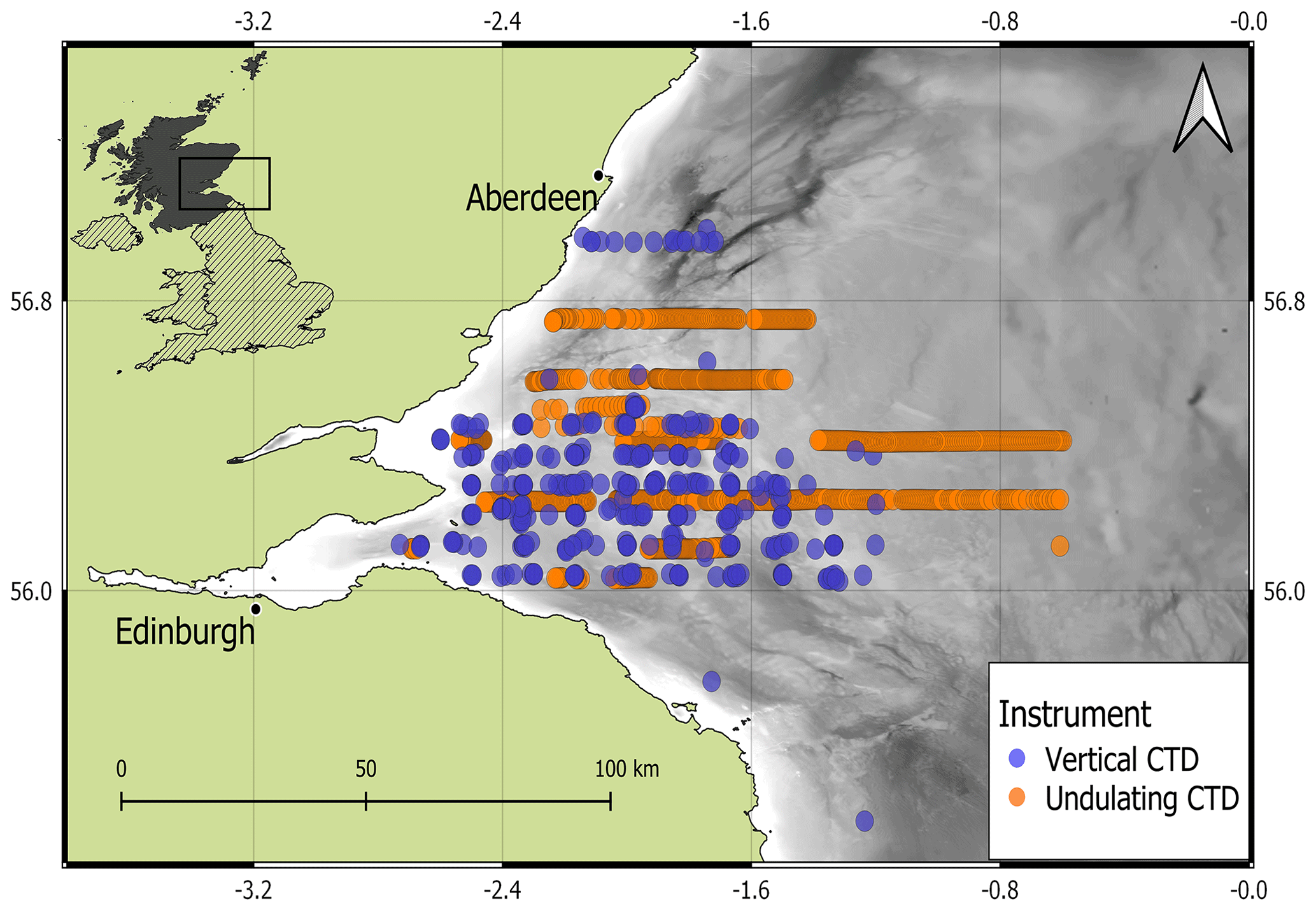
Figure 1 Study area with in situ surveys measured by a vertical CTD (blue dots) and an undulating CTD (orange dots). Land (green) and bathymetry (grey colour ramp) are pictured (EMODnet, 2018).

2.2 Standardized density profiles

Since the proposed algorithm works with profiles at high vertical resolution (1 m), the in situ casts must be standardized throughout the water column. Density (ρ) (kg m⁻³) observations taken every 0.5 to 1 m from the undulating CTD-fluorometer were converted into measurements over regular depth intervals by smoothing and interpolating. This was achieved by fitting a generalized additive model (GAM; Hastie and Tibshirani, 1990) using an adaptive spline with ρ as a function of depth. The obtained smooth function for each profile was used to interpolate ρ at regular 1 m depth intervals. In order to maintain the same shape and values in each profile, the fitted curves at 1 m intervals were visually checked by plotting the estimated and real profiles to identify possible errors visually. 4.16 % of the shapes (n=53) were manually corrected by changing the number of knots in the GAM, which ranged from 75 % to 90 % of the number of observations occurring within each profile. An example is given in Fig. A2 in Appendix A. The analyses were run in R (R Core Team, 2021) using the mgcv package.

2.3 MLD and BMLD detection

2.3.1 Definition of MLD and BMLD

In stratified shelf waters, the layers above and below the pycnocline are mixed vertical region where the density gradient is significantly different from the pycnocline. The upper mixed layer depth (MLD) and the bottom mixed layer depth (BMLD) are both transition regions between mixed waters and the pycnocline (Fig. 2). The most common threshold methods (see Sect. 2.4) identify MLD and BMLD based on the principle that the mixed layer at the surface has a density variance close to zero, which separates it from the pycnocline, exhibiting a larger density gradient. The above assumptions may not always hold, especially when the upper mixed layer is heterogeneous with nested sub-structures such as small re-stratification at the surface or when the pycnocline includes a thin mixed layer (Fig. A1a, e, f in Appendix A) or presents different density gradients (stratified layers) within it (Fig. A1b and c). Such density conditions are difficult to isolate with the available methods.

In the proposed algorithm, the detection of MLD does not assume only that the upper mixed layer has a density gradient close to zero up to the top of the pycnocline, and it firstly identifies MLD (and BMLD) regardless of any a priori thresholds (Chu and Fan, 2019, 2011; Holte and Talley, 2009). Two approaches, the angle method from Chu and Fan (2011) and K-means clustering analysis (Lloyd, 1982), are used to analyse the vertical distribution of density ρ by comparing the observations to each other in the same profile instead of applying an absolute threshold to all profiles. The algorithm differentiates among three layers in the water column with similar density values (the upper mixed layer, pycnocline, and lower mixed layer; Fig. 2). The MLD represents the shallowest depth up to which the difference of density between adjacent points Δρ is small and similar to the surface. The BMLD is the first depth below the pycnocline from which Δρ is small and is similar down to the seabed. This type of detection based on the density shape allows for identification of unconventional vertical density distributions (Fig. A1 in Appendix A) in stratified waters. It is important to note that this method does not determine whether the water column is stratified and it can be applied to profiles exhibiting a pycnocline described by high-resolution, equally distant observations.

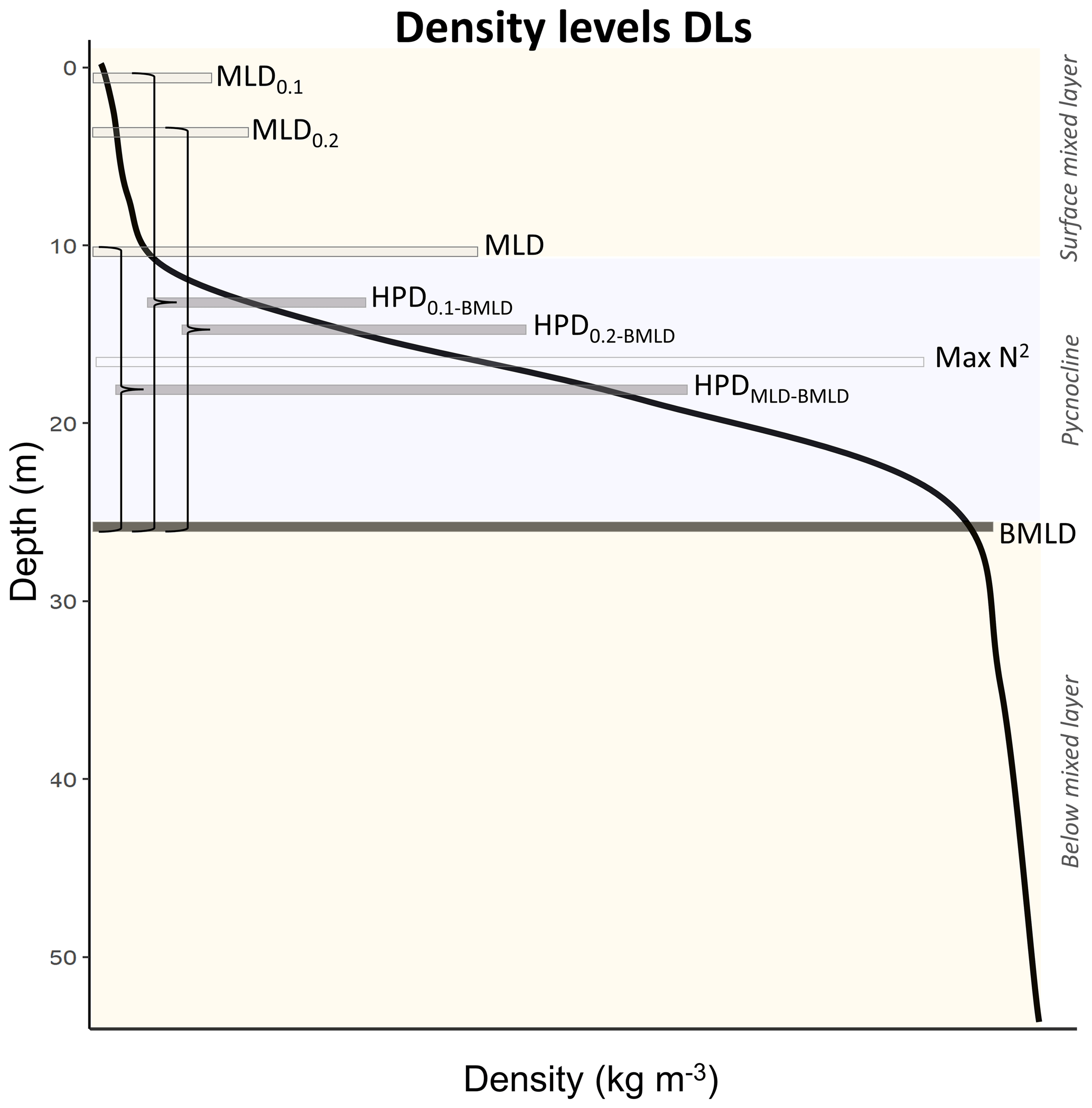
Figure 2 A generic density profile whose limits of the pycnocline (grey rectangle) and surface and below mixed layers (yellow rectangles) are displayed by density levels (DLs). The curly brackets define the halfway pycnocline depths (HPDs) between MLD indicators and BMLD.

2.3.2 Method to extract MLD and BMLD

The algorithm was developed in R (R Core Team, 2021; available at https://github.com/azampollo/BMLD, last access: 3 August 2023) and implements (i) an adaptation of the maximum angle method (Chu and Fan, 2011) and (ii) a cluster analysis on the density difference between two consecutive points ($\mathrm{\Delta }{\mathit{\rho }}_z=\left|{\mathit{\rho }}_z-{\mathit{\rho }}_{z+\mathrm{1}}\right|)$. The method is designed to work with equal, high-resolution (1 m) intervals of density values (z) collected in stratified shelf waters, with a pycnocline defined by more than five values and a BMLD distributed within the first 90 % of the observations from the surface to the deepest point (close to the seabed). The method is sensitive to the number of points within the pycnocline, before MLD and after BMLD, due to the analyses included in the algorithm depending on at least two observations before and after each mixed layer depth.

The first steps of the algorithm follow the method by Chu and Fan (2011), where the depth exhibiting a maximum angle (φ) between two vectors (V1 and V2), referring to density conditions above and below it, is selected as the mixed layer depth. At each observation (z) of the density profile, the method calculates the angle φ from the intersection of V1 and V2, each one fitted using a linear regression model that accounts for the vertical distribution of the density values above (for V1) or below (for V2) z. At each z of the density profile, a unique V1 (blue line in Fig. 3) is fitted using z and two points (2δ) above it and a unique V2 (red line in Fig. 3) is fitted using z and two points below it. The angle φ resulting from the intersection of the two lines is measured in degrees using Eq. (1) in the Supplement. Although Chu and Fan (2011) suggested identifying MLD by measuring the tangent of the angle between V1 and V2, we encountered some issues identifying BMLD in the profiles where φ was bigger than 90^∘ and where density slightly decreased below the pycnocline (Fig. A1d in Appendix A). At this point, an angle φ is associated with each observation in the density profile. Since the identifications of MLD and BMLD are both based on the ranking of φ, the selection of one or the other requires splitting the density profile into “surface” (Split1) and “deep” (Split2) observations to avoid any misidentification and interchange between the mixed layer depths. Split1 includes the density values from the surface (z₁) to two measurement intervals (2δ) above BMLD (Fig. 3a), while Split2 extends from 2δ above the halfway depth in the ρ range (0.5$\mathrm{\Delta }\mathit{\rho }=\left(\right({\mathit{\rho }}_{\text{max}}-{\mathit{\rho }}_{\text{min}})/\mathrm{2})-\mathrm{2})$ to the 90th portion of the profile from the surface to the seabed (z_0.9Δρ=90 % of 1ⁿz) (Fig. 3b). The bottom limit of Split2 was defined at z_0.9Δρ following Chu and Fan (2011) to reduce the number of observations close to the seabed. However, the analyses can be extended up to the end of the profile (see https://github.com/azampollo/BMLD, last access: 3 August 2023).

After the selection of the largest angles as potential MLD and BMLD, further K-means clustering analysis (Lloyd, 1982) was used to identify the mixed and stratified layers based on the density difference between two consecutive points (Δρ_z). The cluster analysis satisfied the assumption that similar observations belong to either the mixed or stratified layers. MLD and BMLD were hence selected above the candidates if the observations above and below them belonged to the same cluster. More details regarding the decisional tree of the algorithm are reported in the Supplement. Adding the conditions controlling for a similar density gradient above MLD and below BMLD decisively improved the selection of pycnocline limits in those profiles exhibiting a pycnocline fractured into chunks. Moreover, several trials reported that the exclusive use of the maximum angle method would have biased the selection due to local variation and instability conditions of the water column (Fig. A1b, c, e, f in Appendix A).

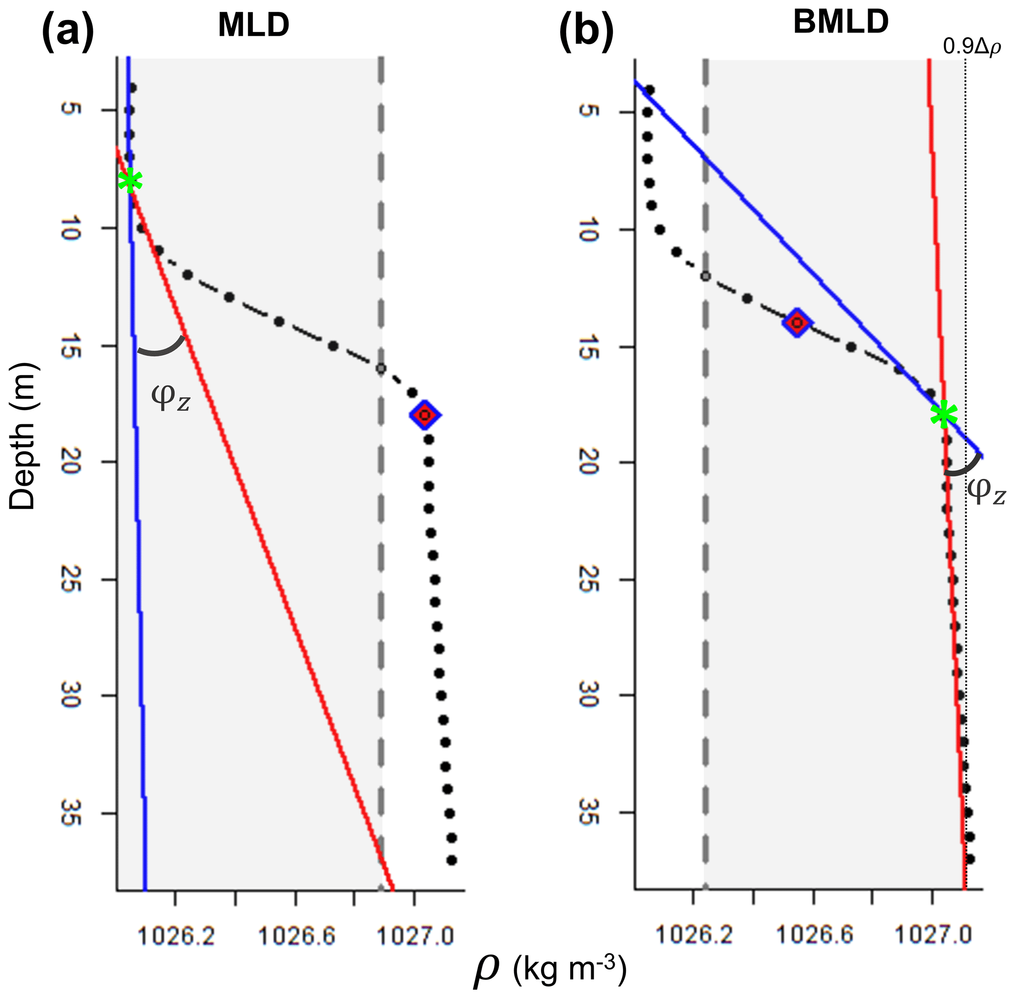
Figure 3 Plots of a density profile reporting the attributes calculated by the algorithm: grey region includes the observations (z; black dots) used to identify (a) MLD within Split1 and (b) BMLD within Split2. Split1 extends from the surface to 2δ above BMLD (purple rhombus), and Split2 from 2δ above half of the profile's density range (0.5Δρ, purple rhombus) to 0.9Δρ. The solid blue and red lines refer to the vectors V1 and V2, whose intersection defines the angle φ_z selected as MLD and BMLD (green stars).

2.3.3 Performance of the algorithm

The algorithm was validated by manually checking the estimated MLD and BMLD in each profile, which were considered wrongly identified when falling into the pycnocline. Since most of the errors located the mixed layer depths clearly at the centre of the pycnocline with thin layers of re-stratification (more than four observations; Fig. A1b, c, e, f in Appendix A), the identifications were considered correct when they appeared (i) on top of a bottom mixed layer (in the BML) and (ii) on top of a large density gradient (pycnocline) separating the surface from deep waters. Major errors in identifying MLD (6.76 % of the profiles) and BMLD (4.32 %) occurred in density profiles with a smooth transition from the mixed layer to the pycnocline, hence reporting a high number of observations at mixed layer depths (e.g. Fig. A1a–c). It is important to highlight the sensitivity of this method to the difference in density (Δρ) at MLD and BMLD (a large Δρ is preferred) and to the sampling frequency at the transition regions between mixed waters and the pycnocline. The algorithm did not correctly identify MLD in profiles with a shallow pycnocline (no upper mixed layer) that comprised two different gradients (Fig. A1c). In this case, the cluster analysis split Δρ within the pycnocline into two groups, although they belong to the same pycnocline. Other errors were related to profiles having a pycnocline split into two parts by a thin mixed layer having more than 4 observations (Fig. A1e). Overall, the identification of BMLD performed better than that of MLD, although it could not handle profiles with fewer than four observations throughout the pycnocline (thickness of the pycnocline <4 m). This condition occurred due to the location of Split2 (which is necessary to distinguish BMLD from MLD selection) (i) at depths above the MLD (misidentifying MLD as BMLD) or (ii) too close to the BMLD (lacking observations to properly fit V1). The algorithm always correctly selected BMLD in profiles with a temporary overturn in the density profile (Fig. A1d).

2.3.4 Common methods identifying density levels (DLs)

The depths detailing the density structure in the water column are defined here as density levels (DLs). Among the multiple indicators of mixed layers that are associated with Chl a vertical distribution, the surface mixed layer depth, the halfway pycnocline depth (HPD), and the maximum squared buoyancy depth were compared to the proposed algorithm identification approaches (MLD and BMLD).

The MLD and BMLD are typically defined in the literature as the depths at which the density exceeds a specific value (threshold method). The threshold is typically selected among a range of values previously tested in the literature (from 0.0025 to 0.125 kg m⁻³) (summarized in Thomson and Fine, 2003; Montégut et al., 2004; Lorbacher et al., 2006; Holte and Talley, 2009) and measured as the difference ($\mathrm{\Delta }{\mathit{\rho }}_z=\left|{\mathit{\rho }}_z-{\mathit{\rho }}_{\text{ref}}\right|)$ between a certain sampling depth (z) and a reference density value (ρ_ref), which can be the density at the surface, at a specific depth (e.g. 10 m), or at a consecutive point (e.g. z−1). In this study, two density thresholds (0.01 and 0.02 kg m⁻³) have been measured as the difference between two consecutive points in the profile ($\mathrm{\Delta }{\mathit{\rho }}_z=\left|{\mathit{\rho }}_z-{\mathit{\rho }}_{z+\mathrm{1}}\right|)$ and are named MLD_0.01 and MLD_0.02.

Since previous studies identified subsurface Chl a in the proximity of the centre of the pycnocline (halfway pycnocline depth, HPD), we investigated the relationship between DCM and three different HPDs measured as the halfway depth between the bottom mixed layer depth (BMLD) and three MLDs identified in this study: HPD_0.01−BMLD (from MLD_0.01), HPD_0.02−BMLD (from MLD_0.02) and HPD_MLD-BMLD (from MLD; Table A1 in the Appendix, Fig. 2).

Moreover, several studies reported positive correlation between the maximum squared buoyancy frequency (Max N²) and DCM at oceanic sites (e.g. Martin et al., 2010; Schofield et al., 2015; Carvalho et al., 2017; Courtois et al., 2017; Baetge et al., 2020) and shelf waters (Lips et al., 2010; Zhang et al., 2016). Therefore, the depth of Max N² has been selected from N² profiles using the gsw package (Kelley and Richards, 2022) in R (R Core Team, 2018) following the most recent version of the Gibbs equation of state for seawater in TEOS-10 systems. The magnitude of N² quantifies the stability of the water column and pinpoints the stratified layers where the energy required to exchange water parcels in the vertical direction is at a maximum (Boehrer and Schultze, 2009).

2.4 Subsurface Chlorophyll a parameters

Deep Chl a maxima (DCMs) were defined as the deepest maximum inflection point in the Chl a profile with 1 m sampling frequency (Carvalho et al., 2017; Zhao et al., 2019). Here, the inflection point is defined as the depth exhibiting a high concentration of Chl a and a large change in Chl a values throughout the profile. The DCM was investigated using the adapted Chu and Fan (2011) method, identifying φ described in Sect. 2.3. The angle φ was measured at each depth of the Chl a profile, and the largest angle with the greatest Chl a concentration was selected as DCM. The automated identification of DCM was checked manually by visual inspection of each profile. The method is available under the function maxChla.R (R Core Team, 2021) at https://github.com/azampollo/BMLD (last access: 3 August 2023).

Depth-integrated Chl a was measured using trapezoidal integration (Walsby, 1997) throughout the water column.

2.5 Evaluating the association of density levels with subsurface Chl a

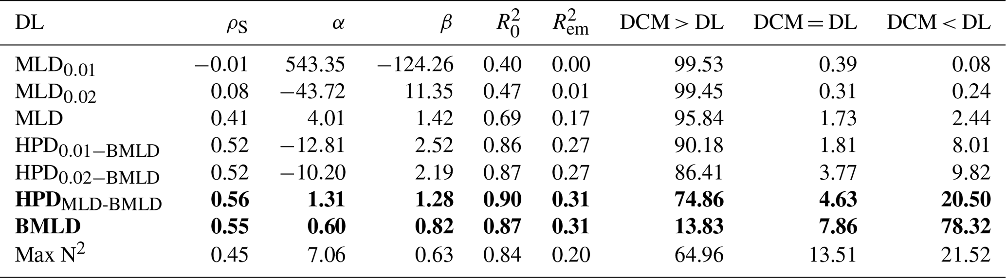
The proximity of each density level (DL) to subsurface aggregations of Chl a was evaluated by comparing their coincidence with DCM (e.g. DCM = BMLD) and their strength in predicting DCM. In this study, we investigate the use of the surface mixed layer depth (MLD_0.01, MLD_0.02, MLD), the maximum squared buoyancy depth (Max N²), and the halfway pycnocline and bottom mixed layer depths (HPD_0.01−BMLD, HPD_0.02−BMLD, HPD_MLD-BMLD, and BMLD) to derive (i) the vertical distribution of Chl a by using the Spearman rank correlation coefficient (ρ_S) and major axis line fitting and (ii) the prediction of DCM from DL by using a linear regression model. All three methods differently assess the correlation or prediction. The Spearman coefficient (Eq. 1 in Table 1) finds a monotonic linear relationship with values ranging between −1 and +1, which refer to a perfect negative or positive correlation between two variables. Besides the strength of the linear relationship defined by ρ_S, we focused on evaluating the linear relationship between DCM and each DL using three different linear models of $y=\mathit{\alpha }+\mathit{\beta }x$: (1) α and β estimated by linear regression, (2) α and β estimated by major axis line fitting, and (3) one-to-one linear regression with α and β fixed at 0 and 1 respectively. The one-to-one line hypothesizes that DCM and DL occur at the same depth. The major axis regression is largely used to investigate how one variable scales against another by assuming that the departures from the fitted line in both directions (x and y) have equal importance (details in the review (Warton et al., 2006). Therefore, the aim of the analysis is not to predict the y variable but to evaluate whether the line-of-best-fit measured by the major axis corresponds to the one-to-one line where any DL equals DCM. The coincidence of each DL and DCM was summarized by reporting the α and β coefficients, which are hypothesized to be intercept ∼0 and slope ∼1 when DCM occurs at the same depth of the DL in question.

Since the identification of drivers for subsurface Chl a represents a useful tool for correctly assessing the abundance and the variations of primary production, we investigated the power of prediction of DCM from each DL by measuring the R squared (R²) from (i) an ordinary least square to estimate parameters from the observations in a linear regression (Eq. 2 in Table 1) and (ii) the one-to-one linear regression (which has been forced with the intercept through the origin and a slope equal to 1; Eq. 3 in Table 1). The equations used to calculate the coefficient of determination R² for the one-to-one ($R_{\mathrm{0}}^{\mathrm{2}})$ and empirical ($R_{\text{em}}^{\mathrm{2}})$ linear regressions are summarized in Eqs. (2) and (3) in Table 1.

Table 1 Equations for estimating the bivariate line-fitting. Spearman rank correlation coefficient (ρ_S) and coefficient of determination R² for testing one-to-one linear regression ($R_{\mathrm{0}}^{\mathrm{2}})$ (e.g. DCM ≈ BMLD) and empirical linear regression ($R_{\text{em}}^{\mathrm{2}})$.

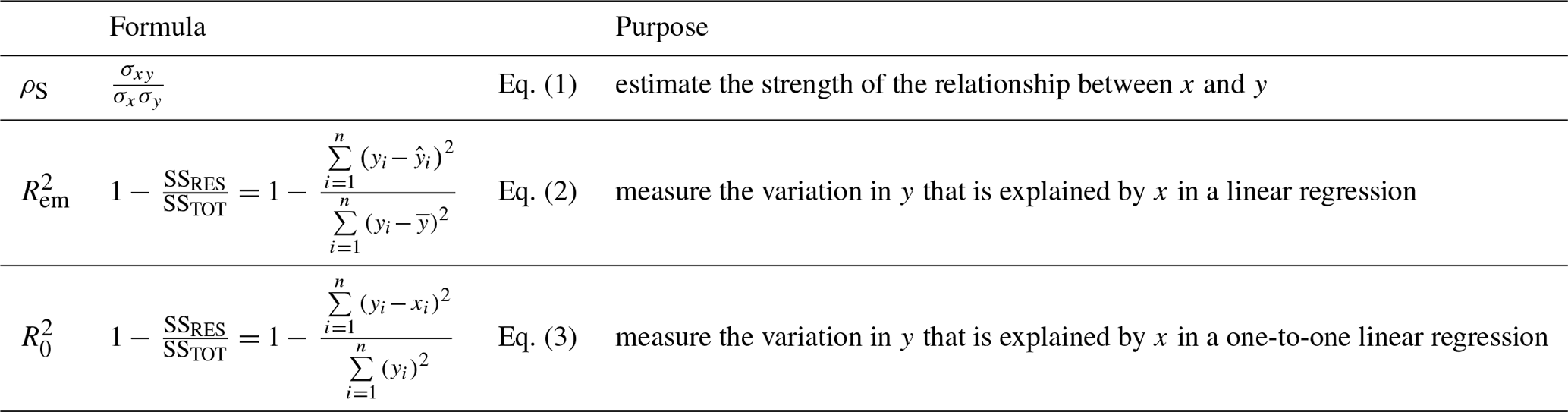
σ_xy is the covariance of x and y, σ_x and σ_y are standard deviations, n is the number of observations of x and y, y_i is DCM_i, $\stackrel{\mathrm{‾}}{y}$ is the average of DCMs, and x_i is the density layers related to DCM in each regression (e.g. BMLD). SS_RES is the residual sum of squares, and SS_TOT is the total sum of squares.

In the empirical linear regression, $R_{\text{em}}^{\mathrm{2}}$ was calculated using the typical equation with the residual sum of squares (SS_RES) as the square of the difference of y and $\widehat{y}$ (estimated y from the model; Eq. 1). In the one-to-one linear regression, SS_RES in $R_{\mathrm{0}}^{\mathrm{2}}$ was adapted by replacing $\widehat{y}$ with x (Eq. 3) since the values of x and y are assumed to be equal in the one-to-one line regression and the difference between them should be zero. The two R² also differ for the denominator SS_TOT, which is the sum of squares about the average of the explanatory variable in $R_{\text{em}}^{\mathrm{2}}$ and the sum of squares of the DCM values since in $R_{\mathrm{0}}^{\mathrm{2}}$ the DCM and DL values are equal.

Since the SS_TOT value adopted in the two equations is different, the proportion of explained DCM variance by each DL can be compared only within each linear regression rather than across the one-to-one and empirical regressions. Therefore, the power of prediction among DLs was discussed for each type of linear regression.

3 Results

The proposed hybrid method identifying MLD and BMLD was applied to 1273 profiles exhibiting a pycnocline. The associations of the density levels (MLD_0.01, MLD_0.02, MLD, HPD_0.01−BMLD, HPD_0.02−BMLD, HPD_MLD-BMLD, BMLD, and Max N²) with DCMs and the vertical distribution of Chl a are described.

3.1 Vertical distribution of DCM and density levels

Deep Chl a maxima (DCMs) were compared to different structures of the density profile that are summarized in surface mixed layer depth (MLD_0.01, MLD_0.02, MLD), bottom mixed layer depth (BMLD), the centre of the pycnocline (HPD_0.01−BMLD, HPD_0.02−BMLD, HPD_MLD-BMLD), and the depth of maximum buoyancy frequency squared (Max N²) to evaluate (i) the vertical distribution of Chl a above and below each DL, (ii) the strength of the positive linear relationship between each DL and DCM, and (iii) the prediction of DCM from each DL.

The observations carried out in the FoF and Tay region confirmed the subsurface presence of maxima Chl a between April and August, with DCMs distributed on average (± standard deviation) at 19.29 ± 6.56 m. All indicators classifying the surface mixed layer (MLD_0.01, MLD_0.02, and MLD) were generally distributed shallower than DCMs (Fig. 4a–c, Table 2), with a rare coincidence of their vertical distribution (from 0.39 % to 1.73 % of the profiles; Table 2). In particular, the threshold methods used to identify MLD exhibited the lowest Spearman correlation amongst all DLs, having almost zero correlation with DCMs (${\mathit{\rho }}_{\text{S}}=-\mathrm{0.01}$ and 0.08 for MLD_0.01 and MLD_0.02; Table 2) and a limited contribution to defining DCM variability in empirical linear regressions ($R_{\text{em}}^{\mathrm{2}}=\mathrm{0.00}$ and 0.01; Table 2). The major axis regression measured intercepts and slopes in MLD_0.01 and MLD_0.02 as being almost perpendicular to the y axis due to the strong presence of DCMs in deep waters. Although a clear subsurface aggregation of Chl a maxima occurs below the surface mixed layer (Fig. 4c), the MLD identified by the algorithm presented in this study was more correlated with DCM than MLD_0.01 and MLD_0.02, with a positive linear relationship between the two variables and a greater explained variance of DCM by using the one-to-one and empirical linear regressions (Table 2). The coefficients of the major axis fitted line for MLD (Table 2) showed a positive correlation of DCMs, representing a gradual deepening of DCM with the top of the pycnocline.

Max N² is the density level performing least well after the MLDs in predicting DCMs, although it showed the highest percentage of coincidence with DCMs (13.51 % of the profiles; Table 2). Similar to MLDs, DCMs have been recorded in 64.96 % of the profiles at layers deeper than Max N², indicating that Chl a maxima area located in waters below surface mixing and below stratified layers within the pycnocline.

Overall, the centre of the pycnocline (HPDs) performed better than MLD and Max N² and were distributed closer to DCMs. HPD_MLD-BMLD showed the highest correlation with DCMs (ρ_S=0.56), and the highest explained DCM variance from the one-to-one ($R_{\mathrm{0}}^{\mathrm{2}}=\mathrm{0.90}$) and empirical ($R_{\text{em}}^{\mathrm{2}}=\mathrm{0.31}$) linear regressions (Table 2). The location of DCMs is highly related to HPD_MLD-BMLD, although only 4.63 % of the profiles presented DCMs and HPD_MLD-BMLD at the same depth (Table 2). Many profiles exhibited DCM deeper than HPD_MLD-BMLD (78.69 %), of which 81.53 % distributed DCMs above BMLD (hence, between HPD_MLD-BMLD and BMLD). HPD_0.01−BMLD and HPD_0.02−BMLD were less related to DCMs in Spearman correlation, major axis, one-to-one, and empirical linear regressions than the HPD_MLD-BMLD (Table 2).

The BMLD exhibited a reverse condition compared to the other density levels by encompassing 78.32 % of DCMs in waters above it (Table 2). BMLDs have the second highest correlation, after HPD_MLD-BMLD, with DCMs (ρ_S=0.55). It is distributed at the same depth of DCMs in 7.86 % of the profiles and linearly predicted the location of Chl a maxima in both one-to-one and empirical linear regressions (Table 2). BMLD exhibited major axis coefficients (α=0.60 and β=0.82) close to the hypothesized one-to-one fitting-line (α=0 and β=1), indicating a good approximation of DCMs close to the base of the pycnocline. Moreover, DCMs were distributed on average at 2.74 ± 5.21 m above BMLD, with a maximum distance above and below it of 22 and 27 m respectively.

The overall distribution of DCMs is mainly discernible (>95.84 % of profiles) below the surface mixed layers (MLD indicators), within the deepest half of the pycnocline (between HPD_MLD-BMLD and BMLD) and it is bounded for 78.32 % of the observations above the BMLD. Although DCMs generally reflect the region with the highest concentration of Chl a throughout the water column, the vertical distribution of Chl a can vary in the proximity of DCMs and accumulate mainly above or below it. Hence, the proximity of the density levels (DLs) to DCMs has been investigated along with the vertical distribution of Chl a (Sect. 3.2).

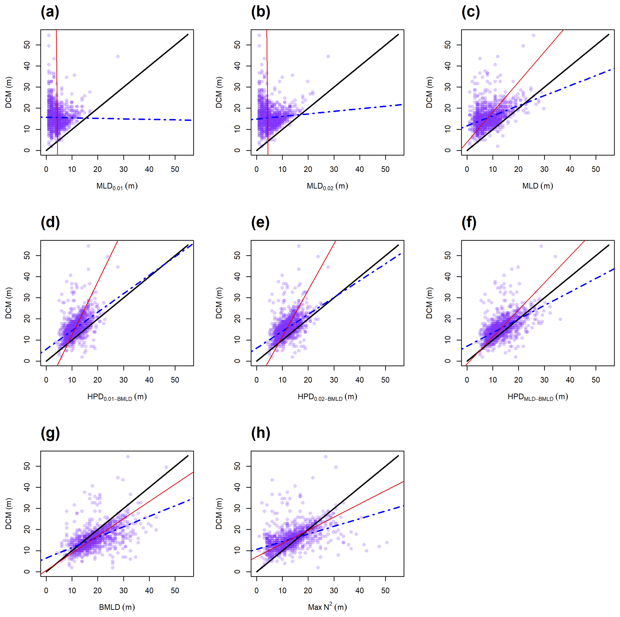
Figure 4 Scatterplots on the locations of DCM and the eight density levels (a–h). The lines refer to the one-to-one linear regression (solid black), the major axis regression (solid red), and the empirical linear regression measured from the observations (DCM ∼ DL; dash-dotted blue). A good relationship between DL and DCM is exhibited in the similar slope and intercept as the solid black line.

Table 2 Statistical parameters and percentage of profiles having DCMs above (>), at the same depth (=), or below (<) each DL. A good relationship is described by an α∼0 and β∼1, high values of ρ_S, $R_{\mathrm{0}}^{\mathrm{2}}$, and $R_{\text{em}}^{\mathrm{2}}$. In bold, the density levels reporting most coinciding with subsurface Chl a maxima.

3.2 Chl a vertical distribution in relation to density levels

Although DCMs generally reflect the region with the highest concentration of Chl a throughout the water column, large concentrations can still accumulate above or below it. Hydrodynamic and biological conditions generating resuspension, passive drift, and mortality (i.e. zooplankton grazing in stratified waters) can shape Chl a differently throughout the water column. Hence, the relevance of the density levels has been investigated in comparison with the vertical distribution of Chl a.

The sum of depth-integrated Chl a (mg m⁻²) of all profiles was standardized by the number of sampling intervals (m) above and below four DLs (MLD, HPD_MLD-BMLD, BMLD, and Max N²). MLD and HPD_MLD-BMLD were selected amongst the density levels to represent the surface mixed layer and the centre of pycnoclines because of their greater correlation with DCM (Table 2). The total amount of Chl a above and below the four density levels is reported as standardized depth-integrated values in Table 3 and shown at each metre of depth in Fig. 5.

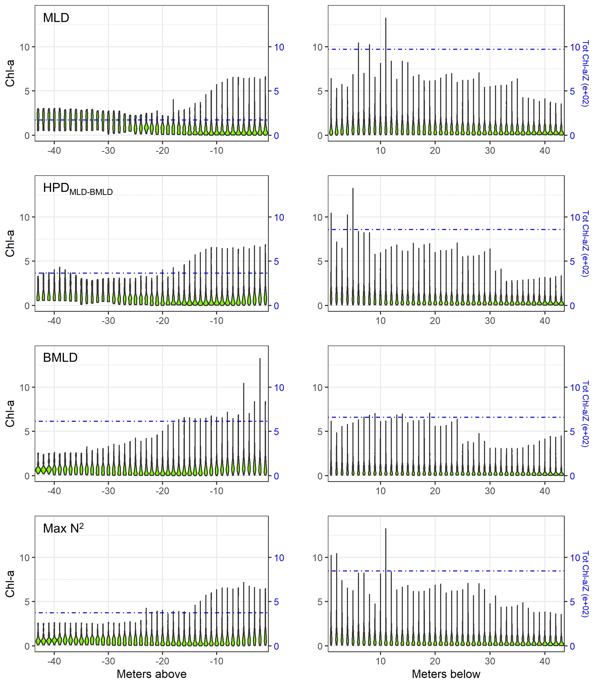
Figure 5 Violin plots of Chl a (mg m⁻³) at each sampled depth above and below the four density levels (MLD, HPD_MLD-BMLD, BMLD, and Max N²) for the whole dataset. The dash-dotted blue lines represent the standardized depth-integrated Chl a measured as the total amount of Chl a from all profiles (mg m⁻²) divided by the number of sampling intervals above or below the DLs.

Table 3 Sum of all depth-integrated Chl a (mg m⁻²) standardized by the number of observations above and below the four density layers.

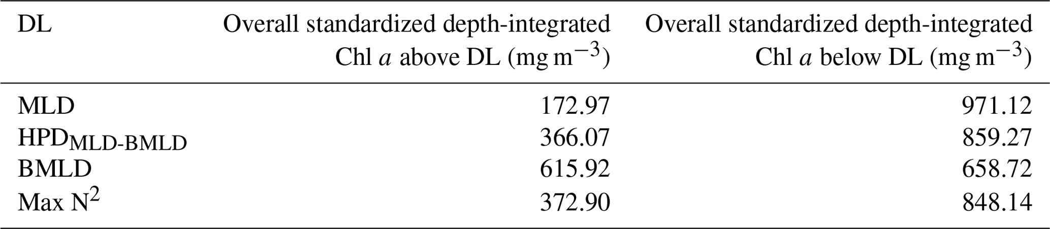
Following the results in Sect. 3.1, a large portion of Chl a was measured at depths below MLD, HPD_MLD-BMLD and Max N² (Table 3), where deep Chl a maxima also occurred. From the seabed to HPD_MLD-BMLD and Max N², the amount of Chl a was 3 times that of the concentrations within the surface and these DLs. The reverse occurred for Chl a distributed above and below BMLDs: the standardized depth-integrated Chl a is higher above BMLDs, although the amount of Chl a in the deepest layers (below the pycnocline) is still comparable (the difference between Chl a from the surface to BMLD and from BMLD to seabed is 42.80 mg m⁻¹) (Table 3).

It is therefore sensible to infer the distribution of DCMs, and the largest portion of Chl a, at depths enclosed within the stratified region (MLD-BMLD), especially in the second half of the pycnocline (HPD_MLD-BMLD-BMLD). At the same time, a noticeable amount of Chl a is still distributed below the pycnocline (BMLD).

4 Discussion

In stratified waters, the vertical distribution of Chl a is regulated by the balance of stratification and mixing across different hydrodynamic regimes over time (van Leeuwen et al., 2015). The combination of static, dynamic, and biological factors (e.g. grazing, Benoit-Bird et al., 2013) induces phytoplankton communities to adapt their vertical distribution at small scales (<1 km, Scott et al., 2010; Sharples et al., 2013). Identifying indicators of subsurface Chl a is essential to investigate the impacts of physical changes due to large-scale factors (e.g. stratification strength, sea-level rise, or turbulence increase downstream wind turbine foundations). To date, several studies have identified the mixed layer between the sea surface and the pycnocline as a valuable tool to assess changes in phytoplankton abundance and phenology, although MLD lacks the ability to provide information on the location of subsurface Chl a in shelf waters. Here we propose a tool to identify the vertical limits of the pycnocline and indicate the bottom mixed layer depth (BMLD) as a key variable influencing the vertical distribution, abundance, and phenology of Chl a in shelf waters.

It is worth noting that the comparison between any DL and DCM was made independent of the timescales at which physical processes and phytoplankton dynamics develop, which differ from each other and do not necessarily overlap. Therefore, the association of any DL with DCM (e.g. BMLD = DCM) was investigated under different physical (e.g. water column stability) and biological conditions (e.g. cell light history regulating photoacclimation), which are likely to be responsible for the unexplained variance reported for each linear comparison in Fig. 4. As an example, the small association of DCMs with all the investigated surface mixed layer indicators (MLD_0.01, MLD_0.02, and MLD; Table 2) could be related to temporal aspects of phytoplankton dynamics and the physical dataset (e.g. multiple data collection within oligotrophic surface waters in stably stratified conditions after spring blooms) at the time of sampling. Hence, the association between any DL and DCM would vary depending on the progression of events defining the profiles of Chl a and density. Here, we discussed the location of DCMs in regard to MLD, HPD, BMLD, and Max N², considering the potential physical conditions and phytoplankton dynamics at the sampling time (such as water column stability, light history exposure, and turbulence) as possible drivers of the resulting associations.

4.1 Association of MLD and Max N² with DCMs

Oceanic sites often exhibit phytoplankton blooms within the upper mixed layer (e.g. Behrenfeld, 2010; Costa et al., 2020; Somavilla et al., 2017). Vertical fluctuations of MLD have been associated with surface phytoplankton blooms caused by the seasonal stratification of temperate waters (Behrenfeld, 2010) or windstorm events deepening the pycnocline into nutrient-enriched waters (Montes-Hugo et al., 2009; Detoni et al., 2015; Carranza et al., 2018; Höfer et al., 2019). Phytoplankton is known to be distributed at the subsurface after blooms, below surface oligotrophic waters (Cullen, 2015), where most of the nutrient input comes from the bottom mixed layer and drives phytoplankton biomass to accumulate at the pycnocline. Since the analysed data in the FoF and Tay region showed DCMs close to the surface (<14 m) in less than 20 % of the profiles, the weak association of DCMs with all the investigated surface mixed layer indicators (MLD_0.01, MLD_0.02, and MLD) could be due to the prevalence of subsurface patches in the dataset, which are likely to be defined by physical dynamics in the bottom rather than the surface mixed layer. In this context, the algorithm returned a measure of the MLD that was correlated more with the DCMs (ρ_S=0.41) than MLD_0.01 and MLD_0.02 (Table 2), the latter distributed above DCMs in >99 % of the profiles. MLD has been considered as a central variable for understanding phytoplankton dynamics in oceanic sites (Sverdrup, 1953), where MLD is mainly informative for surface phytoplankton blooms (Behrenfeld, 2010). This study has shown there is a need for an indicator of the upper limit of the bottom mixed layer, such as BMLD, that can assist further investigation in highly productive but spatially heterogeneous areas such as temperate shelf seas with extensive subsurface aggregations of Chl a.

In the FoF and Tay region, Max N² exhibited higher percentages of coincidence with DCMs (13.51 % of 1273 profiles) than other DLs (Table 2). Max N² is at the depth of a less turbulent region, where the energy to exchange parcels in the vertical is at a maximum (Boehrer and Schultze, 2009). The location of DCMs at Max N² might reflect the distribution of phytoplankton within a less turbulent region where resuspended nutrients by upward fluxes from the bottom mixed layer can persist for longer time periods. Max N² would therefore represent a mild turbulent layer where resuspended phytoplankton cells accumulate, while mixing processes above and/or below Max N² redistribute phytoplanktonic organisms throughout the water column. However, the amount of standardized depth-integrated Chl a below Max N² is almost 3 times greater than above it (Table 3 and Fig. 5), suggesting that Max N² is a small layer with suitable conditions for phytoplankton to grow, but it does not provide information on where most Chl a is vertically distributed. Although the depth of Max N² appeared to better reflect the exact location of DCMs, the percentage of its coincidence with DCMs is still low and might be related to specific conditions at the sampling time (physics and phytoplankton dynamics). Overall, the linear correlation (ρ_S), the major axis coefficients, and the one-to-one linear regression $R_{\mathrm{0}}^{\mathrm{2}}$ described poor association of DCMs with Max N² compared to HPD indicators and BMLD, and hence the use of Max N² to locate subsurface Chl a patches in summertime shelf waters may lead to underestimating the amount of Chl a in the whole water column.

4.2 Vertical distribution of Chl a and BMLD

The observations carried out in the FoF and Tay region confirmed the subsurface presence of maxima Chl a between April and August, which typically develop between the spring and autumn blooms in temperate waters. A study in the German Bight found DCMs to be located mainly at the centre of the pycnocline and that the overall amount of Chl a at depths was distinctly lower than in the surface mixed layers (Zhao et al., 2019). The positioning of the DCM at the pycnocline typically occurs after blooming events deplete nutrients at the surface (Carranza et al., 2018) and is sustained over time by upward nutrient-enriched fluxes entering the pycnocline from deep waters (Pingree et al., 1982; Rosenberg et al., 1990), which are regulated by tidal currents in shelf seas (Palmer et al., 2008). In the Skagerrak Strait between Denmark and Norway, deep SCMs were recorded at a nutricline (rate of change in nitrate and phosphate) located below the base of a shallow pycnocline (<15 m; Bjørnsen et al., 1993). In the FoF and Tay region, only 13.83 % of the profiles reported DCMs below BMLD (Table 2), suggesting that either grazing (Benoit-Bird et al., 2013) and/or deep mixing erode the SCM and redistribute phytoplankton into the bottom mixed layer (Zhao et al., 2019; Sharples et al., 2001). The erosion and resuspension of phytoplankton in deep turbulent waters occurring in the proximity of BMLD, along with the advection of nutrient-enriched waters sustaining new subsurface production, is likely to play a key role in the carbon fluxes of shelf ecosystems (Sharples et al., 2001). Vertical fluctuations of BMLD within and outside the euphotic zone might define whether resuspended cells in the bottom mixed layer are able to photosynthesize under turbulent and low light conditions; e.g. dinoflagellates with swimming velocity <0.1 mm s⁻¹ are able to compete successfully in slightly turbulent conditions (Ross and Sharples, 2007). However, it is important to note that high concentrations of Chl a at DCM in dark waters might reflect the photoacclimation of phytoplankton to low light conditions rather than an actual increase in carbon biomass (Marañón et al., 2021). Photoacclimation is a physiological response to light availability and environmental conditions (Masuda et al., 2021), such as variations in vertical mixing (McLaughlin et al., 2020). Hence, the location of DCM close to the base of the pycnocline reflects a large concentration of pigments rather than of carbon production.

4.3 Using BMLD to investigate ecosystem impacts

In this section, the role of BMLD in future studies is introduced. The linkage between the bottom half of the pycnocline (between HPD_MLD-BMLD and BMLD) and subsurface Chl a suggests BMLD as a key variable for addressing the physical changes in the bottom mixed layer (below the pycnocline), such as those caused by climate changes (e.g. sediment resuspension, shifts in phytoplankton communities, and stratification strengthening) and man-made structures (e.g. increased mixing downstream wind turbine foundations). Identifying BMLD in density profiles allows for measuring the halfway pycnocline depth (HPD), which is highly correlated with DCMs (ρ_S=0.56 Table 2; Holligan et al., 1984; Sharples et al., 2001), and investigating the effects of physical changes on the abundance, vertical distribution, and species composition of primary producers, grazers, and predator species. Future studies could investigate whether pelagic feeders use different structures of the pycnocline (e.g. MLD and BMLD) to detect food patches while diving (e.g. seabirds), and therefore if the variation of these might affect their foraging success.

4.4 Climate change

Since deep turbulent processes sustain primary production in shelf waters under prolonged stratified conditions, changes in the vertical distribution of BMLD can be used to understand the effects of intensified stratification in shelf waters (Capuzzo et al., 2018) such as on the marine food web and physical processes affecting the benthos. Northeast Atlantic shelves have experienced a summertime increase in stratification (increased difference between surface and bottom temperature) with a reduction of nutrient-enriched upward fluxes and a consequential reduction of Chl a in the last 60 years (Capuzzo et al., 2018; Schmidt et al., 2020). Prolonged stratified conditions are known to promote subsurface patches of Chl a (Cullen, 2015) due to the depletion of nutrients at the sea surface after blooms. In the Firth of Forth and Tay region, subsurface concentrations (DCMs) were distributed in the proximity of the deepest portion of the pycnocline, between HPD_MLD-BMLD and BMLD (78.32 % of the profiles), where the weak upward fluxes of nutrients from deep layers are known to sustain the production of Chl a during summer. The limited nutrients at the surface forces phytoplankton to redistribute in the water column (e.g. Boyd et al., 2015; Schmidt et al., 2020) and to photosynthesize in deeper nutrient-enriched waters, typically above the bottom mixed layer and within the euphotic zone. Hence, the role of BMLD as a region of the water column with low turbulence and nutrient-enriched upward fluxes (from the bottom mixed layer) is crucial for phytoplankton productivity within the euphotic zone. The combination of a prolonged stratification over time (Capuzzo et al., 2018), a prolonged isolation of the surface from deep waters, and an increased sediment load (Capuzzo et al., 2015) associated with climate change might affect the vertical distribution of both the pycnocline and the euphotic zone across time and space, consequentially changing the vertical distribution, abundance, and community composition of primary production (Holt et al., 2016, 2018; Capuzzo et al., 2018). The effects of an intensified stratification on primary production suggest an overall reduction of phytoplankton biomass (due to fewer blooms and mixing events after prolonged stratified conditions) and the settlement of Chl a at the subsurface, which are likely to delineate a knock-on effect on redistributing most of the higher trophic levels (e.g. zooplankton, fish) and on changing the foraging success of highly adapted species such as surface-feeding seabirds. Identifying the region (such as between HPD_MLD-BMLD and BMLD) at which subsurface DCMs are typically distributed is therefore important to investigate the potential effects on the ecosystem. For example, the potential deepening of BMLD below the euphotic zone for extended periods will confine deep nutrients from surface euphotic waters, leading phytoplankton biomass to decrease across shelf seas due to the buoyancy of cells at darker depths or in shallow oligotrophic waters. The persistency of stratified conditions is also likely to change the community composition setting at the subsurface close to BMLD, e.g. favouring species coping with low light availability (in a scenario with increased sediment loads). Hence, the region between HPD_MLD-BMLD and BMLD might represent a key section to sample and investigate potential changes related to the composition of phytoplankton and grazer communities. Moreover, the deepening of productive patches might negatively impact global estimates of primary production since remote sensing methods often lack reliability for subsurface data (Jacox et al., 2015), and global carbon sequestration estimates have often failed to include 10 % to 40 % of subsurface Chl a (Sharples et al., 2001). Since the correct measurement of primary production throughout the whole water column is essential, key drivers of subsurface production are necessary to correctly predict, measure, and estimate DCMs from widely used remote sensing data. Although data on the nutricline position were unavailable in this study, the vertical distribution of BMLD provided adequate information on the position of productive subsurface patches in stratified waters, making this variable an important indicator of the vertical distribution of phytoplankton in shelf regions.

4.5 Offshore renewable infrastructure

It is reasonable to stress that potential effects on primary production involve both surface and deep (below the pycnocline) processes, especially where multiple local changes (i.e. close to wind turbine foundations) repeated over large areas (i.e. the North Sea) can have an effect at different scales (van der Molen et al., 2014; De Dominicis et al., 2018; Carpenter et al., 2016). The growing interest of the offshore renewable sector in building offshore wind farms in stratified regions raises the need to draft reliable environmental impact assessments able to identify key variables for estimating the effects in a holistic way (Dorrell et al., 2022). The consequences of offshore wind farms are likely to be related to bathymetry and mixing budgets, by affecting the stratification rate differently across water depths. In this study area with spring tidal speeds <1 ms⁻¹, the vertical distribution of DCMs at BMLDs appeared to be correlated with the bathymetry by exhibiting DCMs closer to BMLDs at water depths of approximately 40 to 70 m, DCMs deeper than BMLD mainly in shallow waters <60 m, and DCMs above BMLD towards deeper waters up to 100 m (Fig. A3 in Appendix A). Previous studies identified a similar pattern in shallow waters (25–85 m), where DCMs were mainly recorded at or below the base of the pycnocline (Barth et al., 1998; Durán-Campos et al., 2019; Holligan et al., 1984; Zhao et al., 2019). Although stratification is reported to intensify in shelf waters with climate change (Capuzzo et al., 2018), the increase in turbulence downstream of wind turbine foundations may counteract local stratification (Carpenter et al., 2016; Schulien et al., 2017; Schultze et al., 2020) and affect the vertical distribution and thickness of the pycnocline across time and space. Moreover, floating wind turbines within the upper water layer (≈25 m) will impact the mixing across density interfaces (Dorrell et al., 2022), and BMLD might represent a useful indicator to vertically locate, on a large-scale, small-scales processes such as scouring and overturning (see Caulfield, 2021). Since the variation in stratification is a useful tool to address possible impacts on primary production, understanding the potential impacts of wind turbine foundations on BMLD and of wind energy extraction on MLD (Daewel et al., 2022) would be useful to efficiently predict changes in the vertical distribution of Chl a and its possible predators.

5 Conclusions

The mixing processes above and below the pycnocline can have very different influences on Chl a vertical distribution, dictating the distribution of subsurface concentrations close to, above, or below the pycnocline. The extent to which subsurface Chl a maxima were distributed in the proximity of a given density level was investigated without a variable controlling for the progression of events affecting the physics and biological dynamics of the water column (e.g. vertical Chl a shape or water column stability) at the sampling time. Hence, the extent of variability retrieved from each comparison (e.g. DCM close to BMLD) is most likely related to the different conditions under which the water columns were investigated, such as the vertical distribution of Chl a (shapes), nutrient availability, stability of the water column (transition from stratified to mixed conditions or vice versa), tidal phase, grazing factors, and phytoplankton dynamics (e.g. cell light history and species composition and competition).

MLD is distributed close to DCMs during surface blooms, explaining the small correlation between MLD and subsurface Chl a in the FoF and Tay region, where a small portion of surface Chl a (<15 m) was collected between 2000 and 2014 (less than 20 % of the profiles). The results indicate that summertime subsurface Chl a maxima are distributed close to HPD and BMLD, indicating that deep processes boosting mixing (such as tidal currents in the North Sea) regulate summer primary production and most of the production above and below BMLDs in respectively deep and shallow waters. Further studies have reported on the key role of the bottom mixed layer in regulating subsurface production and carbon fluxes (Sharples et al., 2001; Palmer et al., 2008), suggesting the BMLD as the vertical depth where the effects of anomaly-inducing processes (e.g. reduced oxygen concentrations below the pycnocline) need to be further investigated. The designed approach is being further developed in order to help in the identification of broad linkages between the physical environment and primary production at finer spatial scales (≤1 km), and a tool to extrapolate this variable from high-resolution vertical profiles in stratified waters is proposed.

Appendix A: List of abbreviations

Abbreviation	Description
BMLD	bottom mixed layer depth (m)
Chl a	Chlorophyll a (mg m−3)
DCM	deep Chlorophyll a maximum (m)
DL	General abbreviation for density level (e.g. MLD, BMLD, HPD, or Max N2) (m)
HPD	halfway pycnocline depth or centre of the pycnocline (m)
Max N2	maximum squared buoyancy frequency (N2; m)
MLD	mixed layer depth or top of the pycnocline (m)
SCM	subsurface Chlorophyll-a maximum (mg m−3)

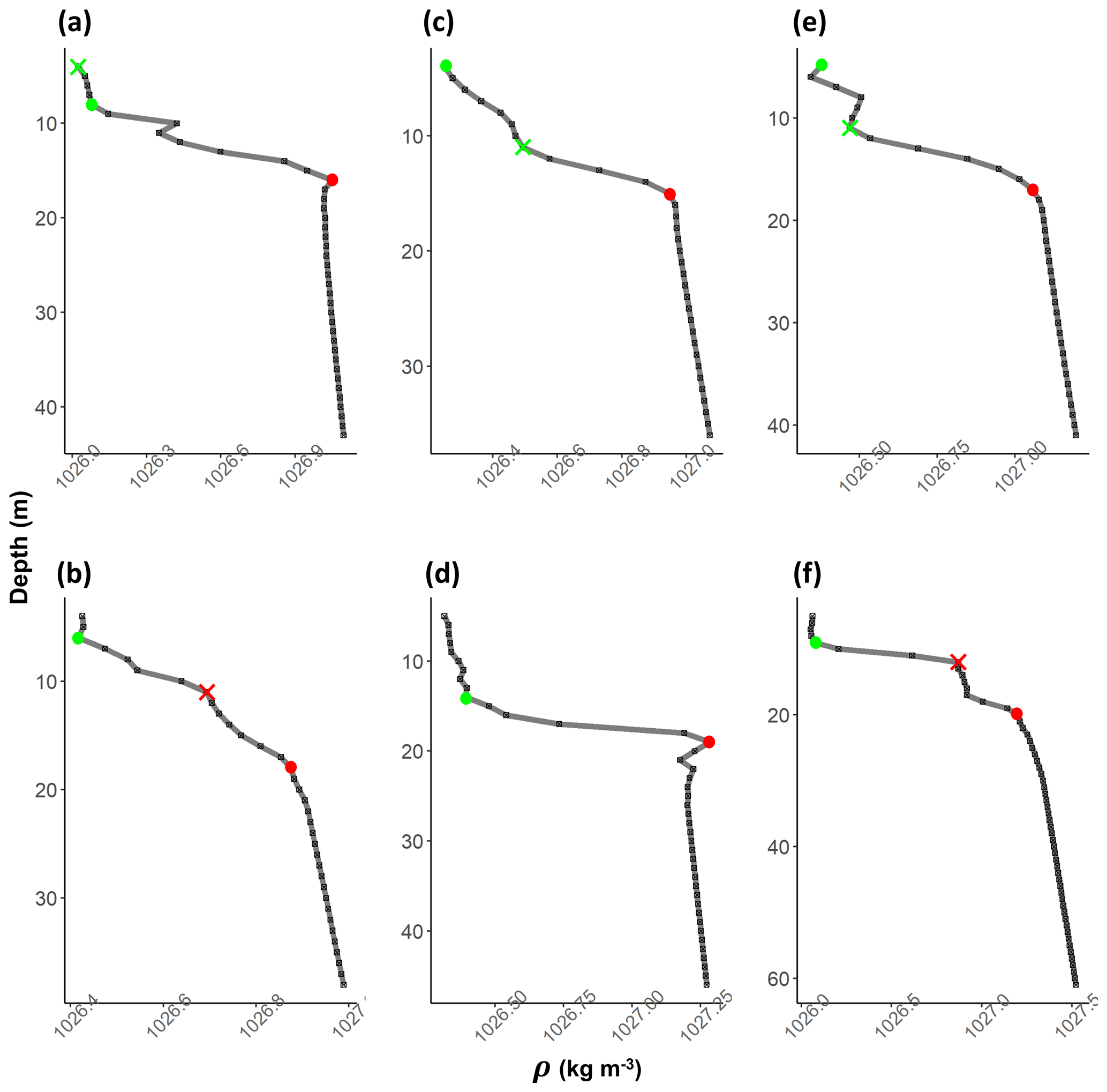
Figure A1 Examples of density profiles (grey line) (a–f). The black squares are observations at 1 m resolution. Red dots refer to BMLD and green dots to MLD. Crosses refer to misidentified MLD (in green) and BMLD (in red) that were manually corrected.

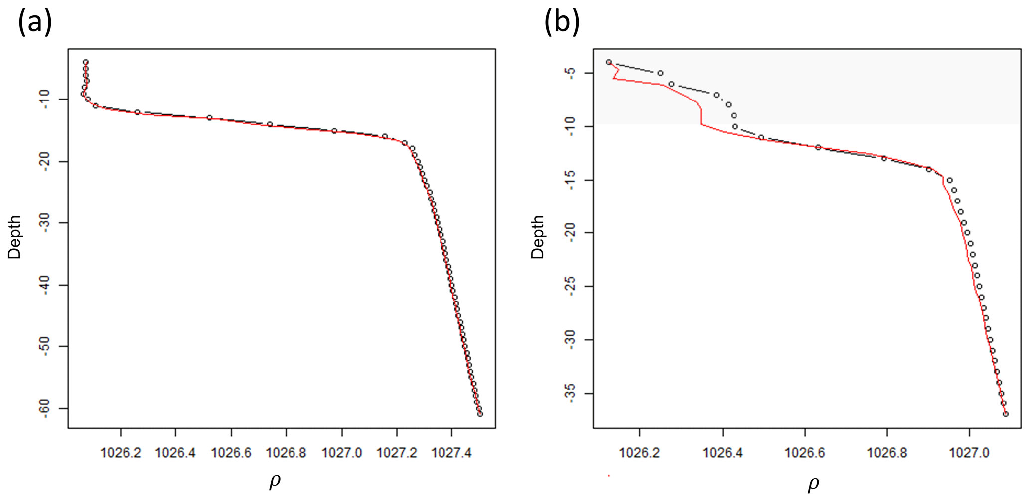
Figure A2 Two density profiles whose observations were standardized at equal 1 m intervals using a generalized additive model (GAM). (a) density profile (black dotted line) where the GAM correctly fitted (red solid line) the vertical distribution. (b) density profile where the GAM wrongly fitted the upper portion of the profile (grey polygon area) and, hence, required manual correction of the values.

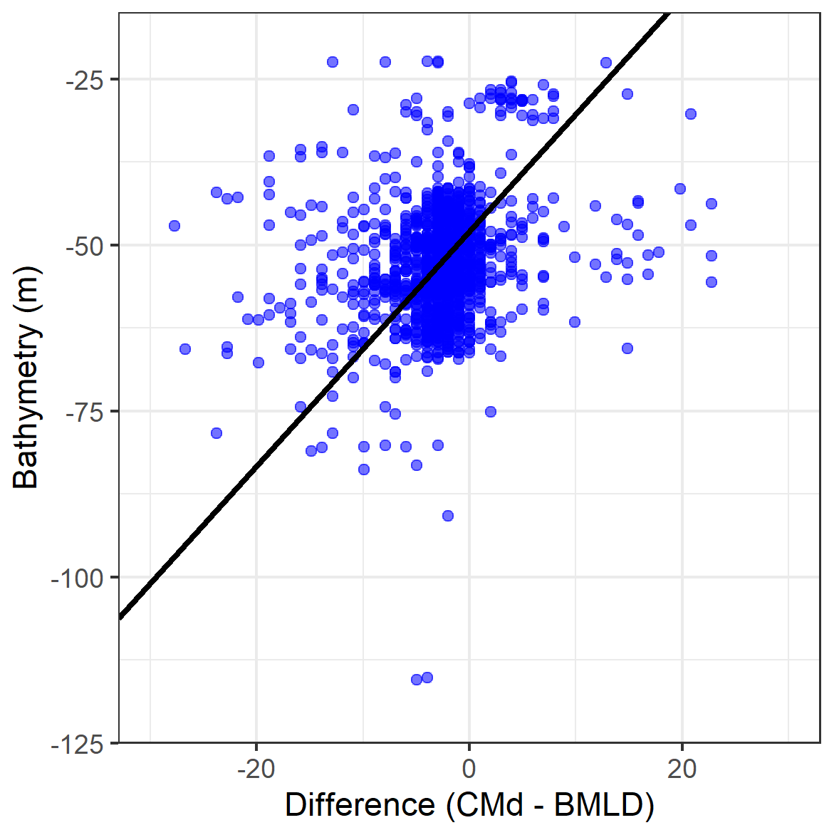
Figure A3 Scatterplot of the difference between DCM and BMLD against the bathymetry at which each profile was sampled. The solid black line reports a standardized major axis regression, whose equation and R squared values are reported.