the Creative Commons Attribution 4.0 License.
the Creative Commons Attribution 4.0 License.
 | 13 Sep 2023
Multiple nitrogen sources for primary production inferred from δ13C and δ15N in the southern Sea of Japan
Taketoshi Kodama
Atsushi Nishimoto
Ken-ichi Nakamura
Misato Nakae
Naoki Iguchi
Yosuke Igeta
Yoichi Kogure
Carbon and nitrogen dynamics in the Sea of Japan (SOJ) are rapidly changing. In this study, we investigated the carbon and nitrogen isotope ratios of particulate organic matter (δ13CPOM and δ15NPOM, respectively) at depths of ≤100 m in the southern part of the SOJ from 2016 to 2021. δ13CPOM and δ15NPOM exhibited multimodal distributions and were classified as belonging to four classes (I–IV) according to the Gaussian mixed model. A majority of the samples were classified as class II (n=441), with a mean ± standard deviation of δ13CPOM and δ15NPOM of ‰ and 3.1 ± 1.2 ‰, respectively. Compared to class II, class I had significantly low δ15NPOM ( ‰, n=11), class III had low δ13CPOM ( ‰, n=21), and class IV had high δ13CPOM ( ‰, n=34). All the class I samples, whose δ15NPOM showed an outlier of total datasets, were collected in winter and had a comparable temperature and salinity originating in Japanese local rivers. The generalized linear model demonstrated that the temperature and chlorophyll-a concentration had positive effects on δ13CPOM, supporting the idea that the active photosynthesis and phytoplankton growth increased δ13CPOM. However, the fluctuation in δ15NPOM was attributed to the temperature and salinity rather than nitrate concentration, which suggested that the δ15N of source nitrogen for primary production is different among the water masses. These findings suggest that multiple nitrogen sources, including nitrates from the East China Sea, Kuroshio, and Japanese local rivers, contribute to the primary production in the SOJ.
- Article
(7097 KB) - Full-text XML
-
Supplement
(1198 KB) - BibTeX
- EndNote


Carbon and nitrogen dynamics in the oceans are globally changing as a result of anthropogenic activities (Gruber and Galloway, 2008). Carbon and nitrogen isotope values (δ13C and δ15N, the differences between the sample isotope ratios ( and ) and standard materials) are particularly effective measurements for detecting changes in marine environments (Gruber et al., 1999; Ren et al., 2017) and ecosystems (Lorrain et al., 2020). Earth-system-model-based techniques have been developed at a global scale in order to comprehend the spatiotemporal variability in carbon and nitrogen isotope values (Buchanan et al., 2019). Marginal seas are strongly affected by anthropogenic activities (Omstedt, 2021). However, because current Earth system models do not focus on them, relevant information is extremely limited.
The Sea of Japan (SOJ) is a western North Pacific semi-closed marginal sea surrounded by the Korean Peninsula, the Japanese Archipelago, and the Russian coast. In the southern part of the SOJ, the Tsushima Warm Current (TWC) flows at the surface (<200 m depth) from the west (East China Sea, ECS) to the east (western North Pacific or the Sea of Okhotsk) throughout the year; however, this current is weak in the winter and strong in the summer, and its path exhibits complex variations (Yabe et al., 2021). The TWC governs the elemental cycles and ecosystem in the southern part of the SOJ (Kodama, 2020), and its water is a mixture of the Kuroshio Current, the Taiwan Warm Current, and Changjiang discharged waters (Isobe, 1999; Guo et al., 2006). The elemental cycles in the surface layer of the SOJ are rapidly changing, and the pH, phosphate, and oxygen concentrations have been decreasing over the past 5 decades (Ono, 2021; Kodama et al., 2016; Ishizu et al., 2019).
Studies in the SOJ have been undertaken using a stable isotope ratio of zooplankton and tissue from small pelagic fish to determine changes in carbon and nitrogen dynamics (Nakamura et al., 2022; Ohshimo et al., 2021). These studies found that the δ13C in animal tissues declined at the same rate as the Suess effect, but there was no significant linear trend in the δ15N (Nakamura et al., 2022; Ohshimo et al., 2021). The δ15N in animal tissues varies with trophic position. In the SOJ, the zooplankton biomass has been found to be negatively coupled with the biomass of small pelagic fish over the last half-century, and, hence, food-web structure may periodically change (Kodama et al., 2022a). Thus, the baseline δ15N in marine ecosystems is vital for identifying changes in nitrogen dynamics in the SOJ. However, reports on the variation in stable isotope ratios of particulate organic matter (POM) in the surface layer, which are the baseline values of marine ecosystems, are confined to the Japanese coastal areas (Antonio et al., 2012; Nakamura et al., 2022). As a result, the variabilities in POM stable isotope ratios with regard to environmental parameters are not clearly understood.
Two recent studies have indicated that the carbon and nitrogen stable isotope ratio of POM varies in the western North Pacific marginal seas (Ho et al., 2021; Kodama et al., 2021). The δ13C of POM increased as the phytoplankton abundance increased in the southwestern ECS, which is consistent with isotope fractionation that occurs during photosynthesis (Ho et al., 2021). The δ15N of this area decreased with freshwater intake and coastal upwelling in the summer and was negatively correlated with nitrate concentration (Ho et al., 2021). Gao et al. (2014) reported the horizontal distribution of δ13C and δ15N and that δ13C largely varies in this sea. Active nitrogen fixation decreases the δ15N of POM in offshore waters in the Kuroshio area during the summer, whereas the δ15N of POM remains high in the coastal waters (Kodama et al., 2021).
The δ13C and δ15N of POM are thought to be more changeable in the SOJ than in the other western North Pacific marginal seas. In the case of carbon, Kosugi et al. (2016) reported that the partial pressure of CO2 (pCO2) on the surface of the central and eastern parts of the SOJ (312–329 µatm) differs from that in the northwestern region (360–380 µatm). Furthermore, the carbon : nitrogen ratio (C : N ratio) of POM in the surface water of the northern ECS is extremely high (> 40 : 1) near Japan (Gao et al., 2014), and this organic carbon-rich water may influence the carbon dynamics of the SOJ. In the case of nitrogen, deep mixing occurs in the SOJ in winter (Ohishi et al., 2019); thus, deep-seawater-originating nitrate contributes to the primary production in the SOJ. The previous nutrient dynamics studies have revealed, however, that the nitrate in the SOJ is supplied from the Kuroshio, regeneration at the bottom of the ECS, the Changjiang diluted waters, and the atmosphere in the summer (Kim et al., 2011; Kodama et al., 2017, 2015). In addition, diazotrophs are present during the summer (Hashimoto et al., 2012; Sato et al., 2021). These “new nitrogen” contributions to the primary production are not evaluated in the SOJ. The primary production in the northeastern ECS is considered to be supported by a variety of nitrogen sources, such as atmospheric deposition, Changjiang River discharge, and Kuroshio waters with varying δ15N (Umezawa et al., 2021, 2014). The decrease in phosphate concentration in the SOJ is mainly observed with an increase in the nitrogen supply in the ECS (Kodama et al., 2016; Kim et al., 2013). Thus, the high contribution of atmospheric deposition, Changjiang River discharge, and Kuroshio waters is expected in the SOJ as well as the northeastern ECS, and the δ15N of POM helps in identifying which nitrogen source mainly supports primary production in this sea. Therefore, in this study, we investigated the carbon and nitrogen stable isotope ratios in the southern SOJ (approximately ≤40∘ N). The main objectives were to (1) demonstrate the spatial distribution of carbon and nitrogen stable isotope ratios and (2) identify which nitrogen source mainly supports the primary production.
2.1 Sampling
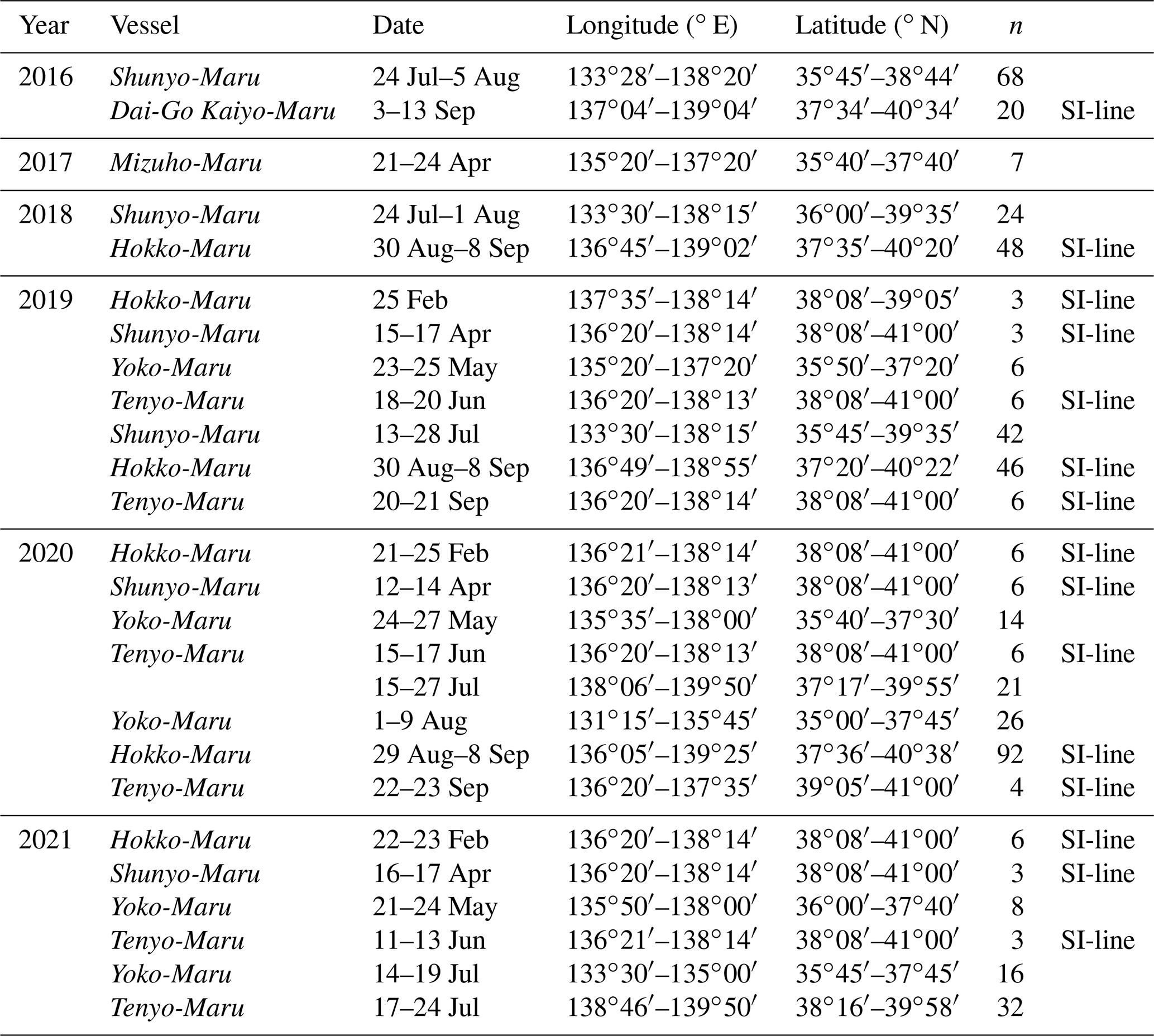
POM samples with environmental data were collected from 2016 to 2021 in the southern part of the SOJ between 35 and 41∘ N and between 131∘15′ E and 139∘50′ E (Fig. 1) during 26 cruises (Table 1). The cruises were held yearly from February to September, except for March (Table 1, Fig. 1). The observations were repeated 15 times after 2016 along the monitoring line established off the Sado Island (SI-line; Table 1, Fig. 1).
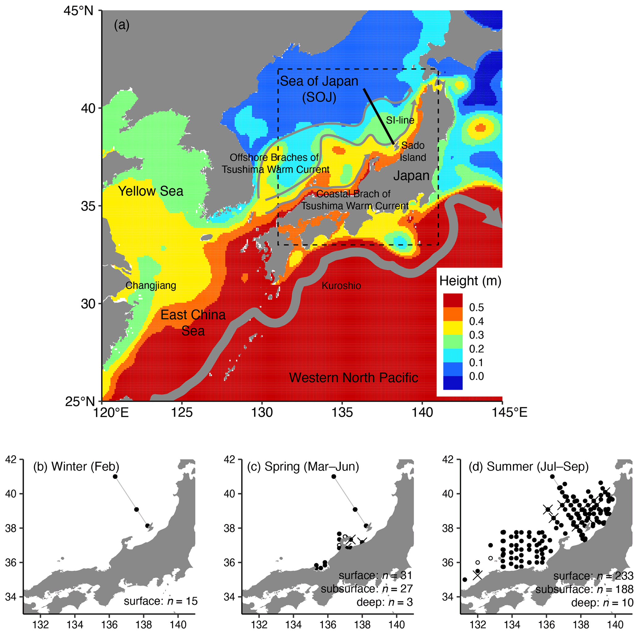
Figure 1Map of the sampling stations. (a) Small-scale map of our observation area (dashed square) with sea surface height and estimated ocean current positions (arrows: two offshore branches of the Tsushima Warm Current, coastal branches of the Tsushima Warm Current, and the Kuroshio). Sampling stations (b) in winter (February), (c) in spring (March–June), and (d) in summer (July–September). The sea surface height was derived from Copernicus Marine Service Global Ocean Physics Reanalysis (GLORYS12V1, https://doi.org/10.48670/moi-00021) in August 2015. Along the SI-line (black solid line in a and gray line in b–d), offshore of Sado Island, repeated observations were made. The crosses indicate the stations where samples were collected from the deep layer (75 m in spring and 100 m in summer), and open circles indicate stations where samples were collected only from the subsurface layer (20–65 m depth). In winter, all the sampling layers were assumed to be in the mixed layer; thus we did not divide them into surface and subsurface layers when collections were made at 10 and 30 m depths. The maps were made with Natural Earth and the Geospatial Information Authority of Japan.
Table 1Summary of the sampling cruises. Date, longitude, and latitude denote their ranges in the cruise, and n means the number of samples. SI-line indicates that the observations were conducted on the SI-line during the cruise, while the collection was also conducted at the other site.
POM samples were generally obtained at the depths of 10 and 30 m or at the subsurface chlorophyll-a maximum (SCM). The vertical profiles of temperature, salinity, and chlorophyll-a fluorescence were monitored in real-time using a conductivity–temperature–depth (CTD) sensor (SBE9plus, Seabird Electronics). Real-time observations were not performed in some specific cases; here, the internally recording-type CTD sensor (SBE19, Seabird Electronics) without a fluorometer was used instead of the SBE9plus. On this basis, we set 30 m as the representative subsurface layer for the spring (March–June) and summer (July–September) seasons as it is below the surface mixed layer in the SOJ. During the cruise in September 2020, the POM samples were collected at six depths (0, 10, 30, 50, and 100 m and SCM) to determine the variations between the sampling layers. In the July and August cruises, photosynthetically active radiation (PAR) was occasionally accessible using a PAR sensor (Seabird Electronics) attached to the CTD. In the summer in the SOJ, the mean (± SD) euphotic zone depth – where PAR is 1 % of the surface – was 50 (± 14) m (n=207), and the PAR at a depth of 30 m was 6.8 ± 4.3 % of that of the surface. In May and August 2020, we collected samples at depths of 75 m (n=3) and 100 m (n=1), respectively. In spring and summer, considering the mixed layer and the euphotic zone depth, the layers at 0–10, 20–65, and 75–100 m depths were defined as the surface, subsurface, and deep layers, respectively, to detect the influence of the vertical difference between unevaluated characteristics such as light and phytoplankton community. In winter, all the samples were regarded as surface layer samples because the difference in potential density between 10 and 30 m depths was <0.125 at every station, suggesting that they were within the mixed layer.
Temperature, salinity, nutrients (nitrate, nitrite, silicate, and phosphate), and chlorophyll-a concentrations were collected and utilized as environmental parameters at the same depth as the POM samples. Water samples were obtained using Niskin bottles mounted on a carousel or a bucket to measure nutrient, chlorophyll-a, and POM concentrations. The nutrient and chlorophyll-a concentrations were analyzed following Kodama et al. (2015). In this study, we only used nitrate concentration because the silicate and phosphate concentrations showed a similar variation to nitrate concentration. The detection limits of the nitrate concentrations were 0.01–<0.1 µM according to the standard deviations of blank values during the measurements. To treat the common-logarithm transformed values, the nitrate concentrations of <0.01 µM (below the detection limit) were set to 0.01 µM. The temperature and salinity at 0 m depth were defined as the values observed by the CTD sensors at 1 m depth because salinity at 0 m depth sometimes exhibited “unreliable” values.
2.2 Isotope analyses
To measure the mass and the carbon and nitrogen stable isotope ratios of POM, 0.9–11.5 L of seawater was filtered using a pre-combusted (450 ∘C, 6 h) glass fiber filter (pore size: 0.7 µm; GF/F, Whatman). The filtration was stopped 2 h after sampling, and >5 L seawater was filtered in 2 h for most of the samples. After the shipboard filtration, the samples were frozen (< −20 ∘C). Onshore laboratory analyses were performed using methods from Kodama et al. (2021), whose preservation differed from that of Lorrain et al. (2003), while the other protocols remained the same. The masses of 12C, 13C, 14N, and 15N were determined using the same sample. The samples were exposed to HCl fumes for >2 h to remove carbonate salt, dried in an oven (60 ∘C) overnight, and stored in a desiccator until isotope ratio measurement. After another round of oven-drying, the entire glass filter was wrapped in a tin cup. Subsequently, the carbon and nitrogen isotope ratios were measured using an Isoprime 100 isotope ratio mass spectrometer (Elementar, Langenselbold, Germany). In 2016, the colored surfaces of the glass filters were scraped off, and the δ13C and δ15N were measured. The absolute amounts of carbon and nitrogen in these scraped samples were different from those in the whole samples. The δ13C and δ15N were calibrated using curves obtained from L-alanine (Shoko Science) during the measurements. The δ13C and δ15N of L-alanine were determined by Shoko Science and regarded as the reference materials (Sato et al., 2014). The δ13C and δ15N of the POM sample (δ13CPOM and δ15NPOM, respectively) were expressed using Eq. (1):
where Rsample and Rreference are the heavy (13C and 15N) to light (12C and 14N) isotope ratios of the POM sample and reference, respectively. The reference materials were atmospheric N2 for nitrogen and Vienna Pee Dee Belemnite for carbon. Given the quality of the L-alanine and the fact that δ13C and δ15N were rounded off to one decimal place, the precision of the analyses was within 0.2 ‰.
The C : N ratio of POM occasionally exhibited outliers, due to which the mean and standard deviations (SDs) of the C : N ratio were calculated and the samples whose C : N ratio differed by more than 3 times the SD of the mean value were eliminated. After elimination, we recalculated the mean and SD of the C : N ratio, and the samples whose C : N ratio differed by >3 × recalculated SD from the recalculated mean value were eliminated. As a result, six samples were removed. Then, the nine samples lacking environmental data were removed. Therefore, 507 samples were used in this study. Among these samples, 101 samples were obtained along the SI-line.
2.3 Statistical analyses
All statistical analyses were conducted using R (R Core Team, 2023). Accompanied by the analysis of variance (ANOVA), a pairwise test with the Tukey–Kramer adjustment was applied to the least-squared mean (lsmean) values. The “ggeffect” package (Lüdecke, 2018) was used to calculate the lsmean values and standard errors (SEs). The “car” package (Fox and Weisberg, 2018) of ANOVA was used to conduct a type-II ANOVA for unbalanced data comparison. Neither δ13CPOM nor δ15NPOM exhibited a normal distribution according to the Kolmogorov–Smirnov test (p<0.001); both showed multimodal distributions. The linear models cannot be applied to the multimodal distributions; we applied a two-dimensional Gaussian mixed model (GMM) to classify δ13CPOM and δ15NPOM using the “mclust” package (Scrucca et al., 2016). The samples were not divided based on the sampling depth and seasons. The Bayesian information criterion (BIC) determined the number of classes.
Generalized linear models (GLMs) were applied to assess the variables that predicted the relationships between the environmental parameters and δ13CPOM and δ15NPOM as in Kodama et al. (2021). We assumed that the error distributions of δ13CPOM and δ15NPOM were normally distributed with a linear link function in the GLMs. The full GLM models are as follows:
where δXPOM, long, lat, , T, S, Chl, and Nit denote δ13CPOM or δ15NPOM, longitude, latitude, the C : N ratio, temperature, salinity, chlorophyll-a concentration, and nitrate concentration, respectively. The chlorophyll-a and nitrate concentrations were transformed into logarithmic values. The arguments of the f functions are categorical variables that are used to simulate non-linear relationships. The numbers of classes were defined by GMM and BIC, while those of layer and season were three each (surface, subsurface, and 100 m depth in layer and winter (January–February), spring (March–June), and summer (July–September) in season). The explanatory variables used in the full GLMs were chosen based on the retraction of multicollinearity. We also used GLM approaches that included a quadratic expression in the model, as Nakamura et al. (2022) did, as well as a generalized additive model approach, as Kodama et al. (2021) did. However, as the deviance-explained values of the models did not improve, we opted for the simple GLM approach.
The explanatory variables and final GLM descriptions were selected using the corrected Akaike information criterion (AIC), which may be used to assess the likelihood of the model. The lsmean values and SEs based on the AIC-selected GLMs were used to visualize the influence of the explanatory variables on the δ13CPOM or δ15NPOM. ANOVA was used to test the effects of the lsmean values of the categorical variables (the class, season, and depth when they remained).
We did not include the interaction terms in the GLMs. For instance, longitude–latitude interactions can reflect the 2-D variations. Moreover, the temperature–salinity (T–S) diagram is the most fundamental method for obtaining the characteristics of water masses. Therefore, although the interactions must be considered, the interaction terms of temperature and salinity could not be used instead of the T–S diagram in the GLMs.
3.1 Spatial distribution of δ13CPOM and δ15NPOM
The δ13CPOM and δ15NPOM varied from −29.3 ‰ to −17.7 ‰ and −3.2 ‰ to 6.7 ‰, respectively. In September 2020, the vertical profiles (0, 10, 30, 50, and 100 m depths and SCM (34–56 m)) of δ13CPOM and δ15NPOM were collected at nine stations. The differences in the δ13CPOM, δ15NPOM, and C : N ratios were significant among the layers according to ANOVA (p<0.001). The δ13CPOM was the lowest at a depth of 50 m or SCM (mean ± SD: −25.7 ± 0.4 ‰ and −25.4 ± 0.5 ‰, respectively; Fig. 2a). The δ13CPOM decreased with a depth of up to 50 m (or SCM layer) and increased slightly at 100 m depth (−24.2 ± 1.3 ‰). The δ15NPOM was the lowest at 10 m depth (1.5 ± 0.6 ‰) and increased with depth, and the highest value was identified at 100 m depth (5.0 ± 0.6 ‰) (Fig. 2b). The mean C : N ratio was estimated to be 5.4–6.3 mol mol−1 except at 100 m depth with 4.2 ± 0.69 mol mol−1 (Fig. 2c). When the subsamples at the nine stations were regrouped into the surface (0 and 10 m depths) and subsurface (30 and 50 m and SCM) groups, the differences in both δ13CPOM and δ15NPOM were significant between the surface and subsurface (t test, p≤0.018). Therefore, δ13CPOM and δ15NPOM were different between the surface and subsurface, particularly during summer.
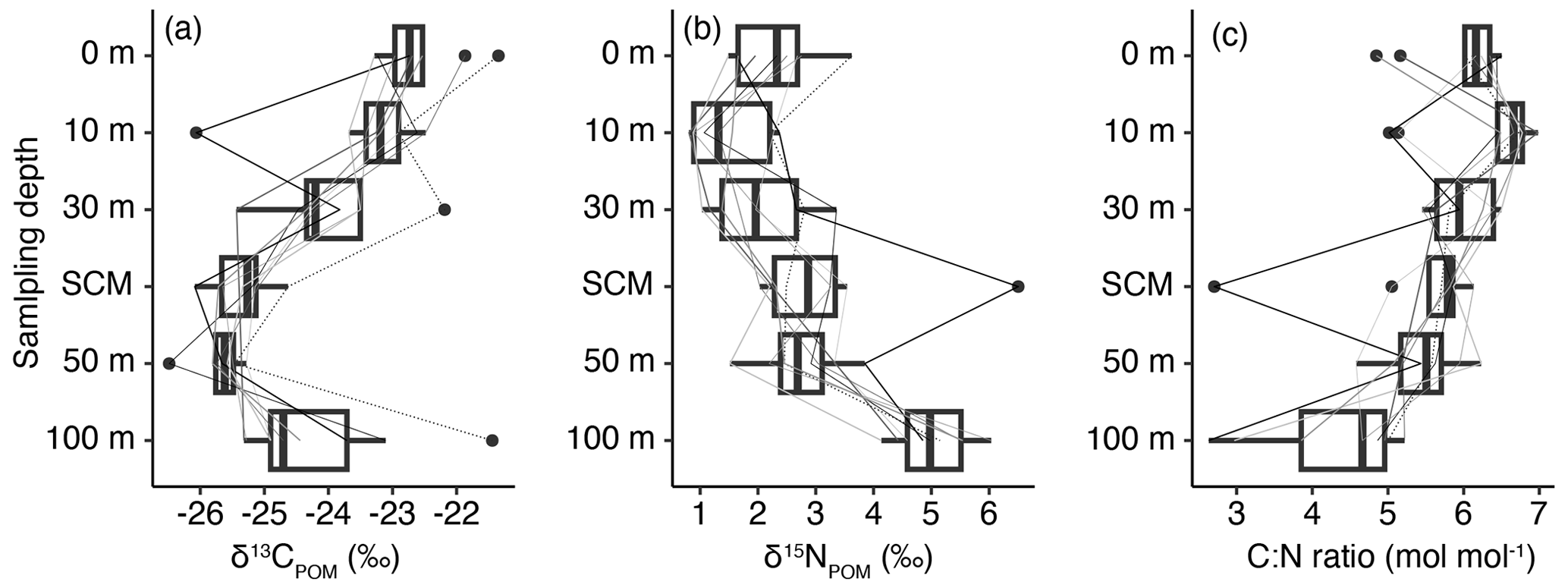
Figure 2The vertical profiles of (a) δ13CPOM, (b) δ15NPOM, and (c) the C : N ratio collected at nine stations in the eastern part of the Sea of Japan during September of 2020 (crosses in Fig. 1). Lines denote the profiles of every station. Box plots show the median (vertical thick lines within boxes), upper and lower quartiles (boxes), quartile deviations (horizontal bars), and outliers (closed circles).
The horizontal variations in δ13CPOM are shown by the 1∘ × 1∘ grid median values (Fig. 3a–e). During winter, the median (± interquartile range, IQR) of the δ13CPOM was −25.0 ± 1.6 ‰, and low δ13CPOM was observed in the offshore waters. During spring, low δ13CPOM was identified offshore, and the surface δ13CPOM (−24.6 ± 1.6 ‰) was lower than that of the subsurface (−23.7 ± 1.4 ‰; Wilcoxon test, W = 271, p=0.021). During summer, the surface δ13CPOM (−22.9 ± 1.0 ‰) was significantly higher than that of the subsurface (−24.4 ± 1.9 ‰; Wilcoxon test, W = 36 002, p < 0.001). The δ13CPOM in the subsurface during the summer was higher in the western than in the eastern part, while those of the surface were higher in the eastern than in the western part.
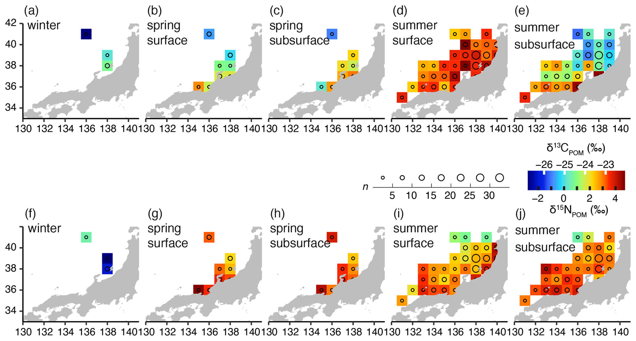
Figure 3Horizontal distributions of δ13CPOM (a–e) and δ15NPOM (f–j) in the Sea of Japan (1∘ × 1∘ grid median values for 5 years). (a, f) Winter, (b, g) the surface layer of spring, (c, h) the subsurface layer of spring, (d, i) the surface layer of summer, and (e, j) the subsurface layer of summer. Circle sizes reflect the sample numbers used for calculating the median values. The maps were made with Natural Earth and the Geospatial Information Authority of Japan.
The horizontal variations in δ15NPOM are shown in the same manner as δ13CPOM (Fig. 3f–j). Evidently, in winter, lower values (∼ −2.0 ‰) were observed. δ15NPOM was higher in spring (3.1 ± 1.8 ‰ and 3.2 ± 0.8 ‰ at the surface and subsurface, respectively) than in winter (−2.0 ± 2.0 ‰). Moreover, during spring, the δ15NPOM value in the offshore area was lower than that of the coastal area. In summer, the surface δ15NPOM (2.8 ± 1.7 ‰) was significantly lower than that of the subsurface (3.1 ± 1.5 ‰; Wilcoxon test, W = 19 187, p=0.02874). Furthermore, lower δ15NPOM values were identified in the offshore water, and high δ15NPOM values were observed in the coastal area of the northern part.
3.2 Temporal variations in δ13CPOM and δ15NPOM along the SI-line
The monthly variations in δ13CPOM and δ15NPOM were evaluated using the samples collected along the SI-line (Fig. 4a–d). When the interannual variations were ignored, δ13CPOM of the surface was the lowest in April (lsmean ± SE: −25.7 ± 0.5 ‰; n=8) and highest in September (−22.3 ± 0.33 ‰, n=23) (Fig. 4a); no significant difference was observed during February, April, and June (pairwise test with Tukey–Kramer adjustment, p>0.05). In the subsurface layer, the monthly variation in δ13CPOM was not significant (ANOVA, p=0.09) (Fig. 4b). The δ15NPOM of the surface layer was the lowest in February (−1.1 ± 0.4 ‰, n=15) and highest in July (3.1 ± 0.5 ‰, n=7), while a significant difference was observed only in February and other months (Fig. 4c). In the subsurface layer, the monthly variation in δ13CPOM was not significant (ANOVA, p=0.09) (Fig. 4b) and that of δ15NPOM was significant (p=0.033), and a significant difference (p=0.025) was observed between April (1.0 ± 0.6 ‰, n=3) and June (3.3 ± 0.4 ‰, n=6, Fig. 4d).
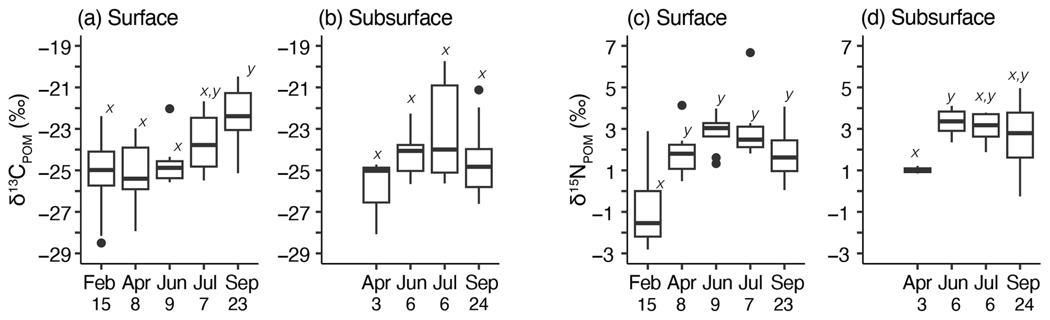
Figure 4Temporal variations in δ13CPOM (a, b) and δ15NPOM (c, d) along the monitoring line (SI-line); (a) monthly variation in δ13CPOM in the surface layer, (b) monthly variation in δ13CPOM in the subsurface layer, (c) monthly variation in δ15NPOM in the surface layer, and (d) monthly variation in δ15NPOM in the subsurface layer. Box plots show the mean (thick horizontal lines within boxes), standard deviation (boxes), maximum or minimum values (vertical bars), and outliers (closed circles). The lower-case italic characters near the boxes (x and y) reflect the results of the pairwise test with Tukey–Kramer adjustment; the same character pairs showed an insignificant difference within the pair (p>0.05). The pairwise test with Tukey–Kramer adjustment was not significant among any pairs of δ13CPOM in the subsurface layer (c). The numbers just below the horizontal axis labels indicate the sample numbers.
3.3 Classifications of δ13CPOM and δ15NPOM
The samples were divided into four classes (I–IV) based on δ13CPOM and δ15NPOM according to the two-dimensional GMM (Fig. 5). The means ± SD of δ13CPOM and δ15NPOM were −24.6 ± 1.2 ‰ and −2.1 ± 0.8 ‰ in class I (n=11), −23.7 ± 1.2 ‰ and 3.1 ± 1.2 ‰ in class II (n=441), −27.1 ± 1.0 ‰ and 2.0 ± 1.3 ‰ in class III (n=21), and −20.7 ± 0.8 ‰ and 1.7 ± 1.0 ‰ in class IV (n=34), respectively (Fig. 5b–c). The δ13CPOM values were significantly different among the different classes (p<0.001, pairwise test with Tukey–Kramer adjustment), except between classes I and II (p=0.06) (Fig. 5b). The δ15NPOM values were significantly different among the different classes (p<0.001, pairwise test with Tukey–Kramer adjustment), except between classes III and IV (p=0.76) (Fig. 5c). However, the mean ± SD values of δ15NPOM in classes III and IV were within the range of class II values (Fig. 5c). Therefore, the characteristics of δ13CPOM and δ15NPOM in classes I, II, III, and IV were middle δ13CPOM and low δ15NPOM, middle δ13CPOM and high δ15NPOM, low δ13CPOM and high δ15NPOM, and high δ13CPOM and high δ15NPOM, respectively.
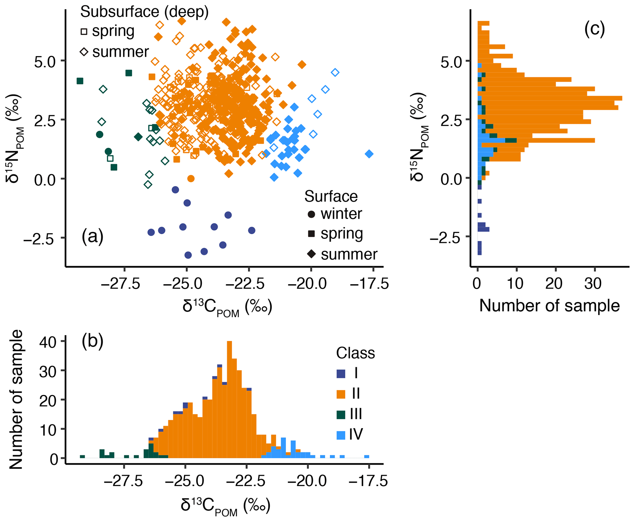
Figure 5(a) Diagram of δ15NPOM and δ13CPOM. Stacked histograms of (b) δ13CPOM and (c) δ15NPOM for the two-dimensional Gaussian mixed model (GMM), with colors indicating the different classes.
Environmental conditions (temperature, salinity, nitrate concentration, chlorophyll-a concentration, and the C : N ratio) differed significantly among the classes (ANOVA, p<0.01; Fig. 6). The temperature was lower in classes I (mean ± SD: 10.1 ± 2.0 ∘C) and III (12.7 ± 6.0 ∘C) than in classes II (20.1 ± 4.9 ∘C) and IV (24.0 ± 2.6 ∘C) (Fig. 6a). Significant differences in temperature were discerned (p<0.003, pairwise test with Tukey–Kramer adjustment) among different classes, except between classes I and III (p=0.44). The only significant difference in salinity among the classes was discerned between classes II (33.76 ± 0.79) and III (34.27 ± 0.18) (p=0.01, pairwise test with Tukey–Kramer adjustment) (Fig. 6b). The mean salinities with SD of classes I and IV were 33.99 ± 0.06 and 33.91 ± 0.36, respectively (Fig. 6b). The mean nitrate concentration values were high in classes I (4.20 ± 1.31 µM) and III (3.88 ± 3.86 µM), lower in class II (0.51 ± 1.31 µM), and the lowest in class IV (0.05 ± 0.01 µM) (Fig. 6c). The chlorophyll-a concentrations were significantly different among the classes (ANOVA, degrees of freedom (DF) = 3, F value = 2.643, p=0.048), but no significant differences were identified among the pairs (p>0.058). The chlorophyll-a concentration was the highest in class IV (0.69 ± 1.33 µg L−1) and was followed by class I (0.61 ± 0.23 µg L−1) and class III (0.58 ± 0.37 µg L−1), and it was the lowest in class II (0.44 ± 0.48 µg L−1) (Fig. 6d). A high C : N ratio was identified in class IV (7.06 ± 1.50 mol mol−1), which was significantly higher (p<0.01, pairwise test with Tukey–Kramer adjustment) than in classes II (6.13 ± 1.39 mol mol−1) and III (5.12 ± 1.22 mol mol−1), while the C : N ratio in class IV did not differ from that in class I (6.05 ± 0.58 mol mol−1) (Fig. 6e).
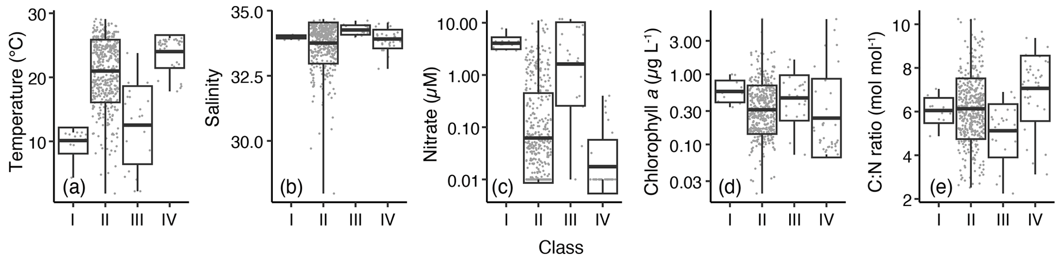
Figure 6Differences in environmental parameters among the classes divided based on δ13CPOM and δ15NPOM. Parameters include (a) temperature, (b) salinity, (c) nitrate concentration, (d) chlorophyll-a concentration, and (e) the C : N ratio. Box plots show the mean (thick horizontal lines within boxes), standard deviation (boxes), and maximum or minimum values (vertical bars). The small gray dots represent the raw values.
The T–S diagram demonstrated that all the samples of class I were observed in winter and mostly (10 of 11 samples) in water with temperature and salinity within the 9.4–11.4 ∘C and 33.877–34.038 ranges, respectively (Fig. 7). Only a single sample of class I was identified at a temperature and salinity of 4.3 ∘C and 34.037, respectively (Fig. 7). The class III samples were never observed above 24 ∘C, and 20 of the 21 samples were observed below 19 ∘C (Fig. 6) but did not group into similar T–S characteristics (Fig. 7). The class IV samples were only observed during summer and plotted in the warm water mass in summer of 2019 but were also observed in the different T–S characteristics in the other year (Fig. 7).
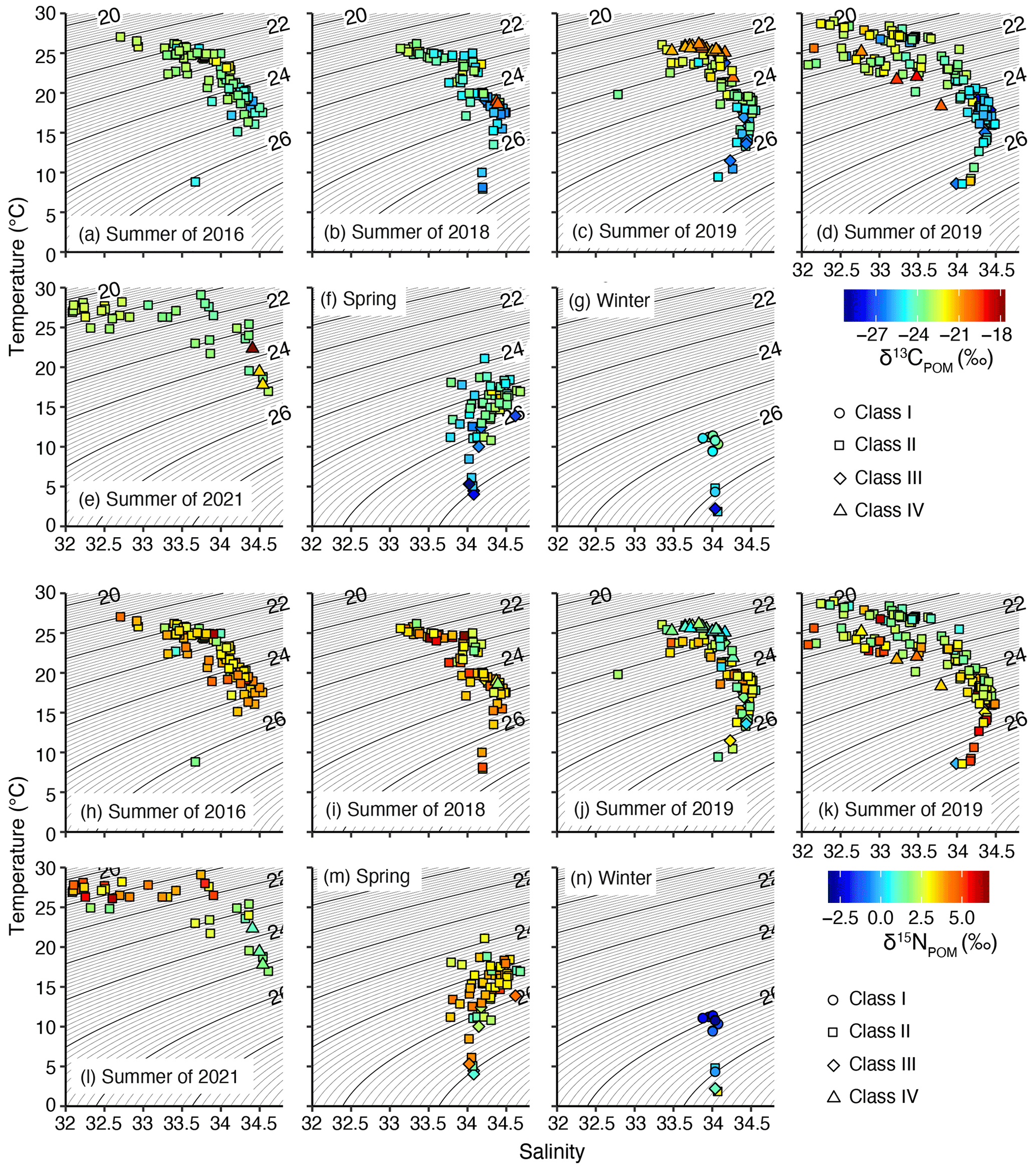
Figure 7T–S (temperature–salinity) diagram overlaid with δ13CPOM (a–g) and δ15NPOM (h–n). Spring (f, m) and winter (g, n) were not divided into observation years. In this diagram, salinity <32 was not plotted. The different symbols indicate different classes.
3.4 Relationships with environmental conditions
According to the GMM, both δ13CPOM and δ15NPOM exhibited multimodal distributions. The linear regression was based on the assumption that the dependent variable has a normal distribution; therefore, in this study, the linear regressions were inappropriate for evaluating the relationships. We have provided the results of the linear regression analysis in the Supplement (Fig. S1).
The least AIC GLM for δ13CPOM was as follows:
The r2 value of the least AIC δ13CPOM model was found to be 0.659. ANOVA indicated that all the remaining explanatory variables were significant (χ2≥7.53, p≤0.006). The responses of latitude, salinity, and nitrate concentration were significantly negative (p<0.001), whereas those of temperature and chlorophyll-a concentration were significantly positive (p<0.001) (Fig. 8). The lsmean δ13CPOM with ANOVA suggested that classes III (lsmean ± SE: −25.6 ± 0.3 ‰) and IV ( ‰) were significantly higher and lower than those of other classes, respectively (pairwise test with Tukey–Kramer adjustment, p<0.001). The difference between classes I (−23.0 ± 0.4 ‰) and II (−23.4 ± 0.1 ‰) was insignificant (pairwise test with Tukey–Kramer adjustment, p=0.542) (Fig. 8a). The δ13CPOM of the surface (lsmean ± SE: −23.4 ± 0.1 ‰) was higher than that of the subsurface (−23.7 ± 0.1 ‰, pairwise test with Tukey's adjustment, p=0.0154). Moreover, δ13CPOM at 100 m depth (−22.4 ± 0.3 ‰) was significantly higher than those of the surface and subsurface (p≤0.001) (Fig. 8).
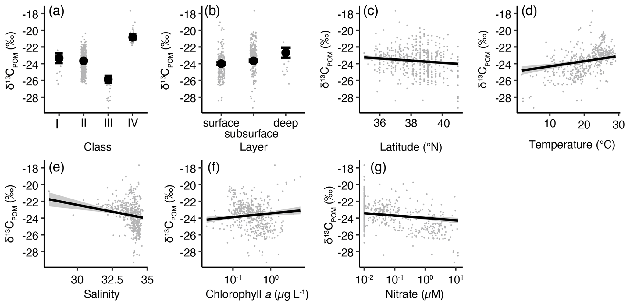
Figure 8The least-square-mean (lsmean)-based effects of the environmental parameters in the least AIC GLM for δ13CPOM. Effect of (a) classes, (b) sampling depth, (c) latitude, (d) temperature, (e) salinity, (f) log-transformed chlorophyll-a concentration, and (g) log-transformed nitrate concentration. Closed circles with bars or solid lines with shadows represent the lsmeans with 95 % confidence intervals. The small gray dots represent the observation data. When necessary, the settings of the class and layer for the calculation of lsmeans were class II and surface, respectively.
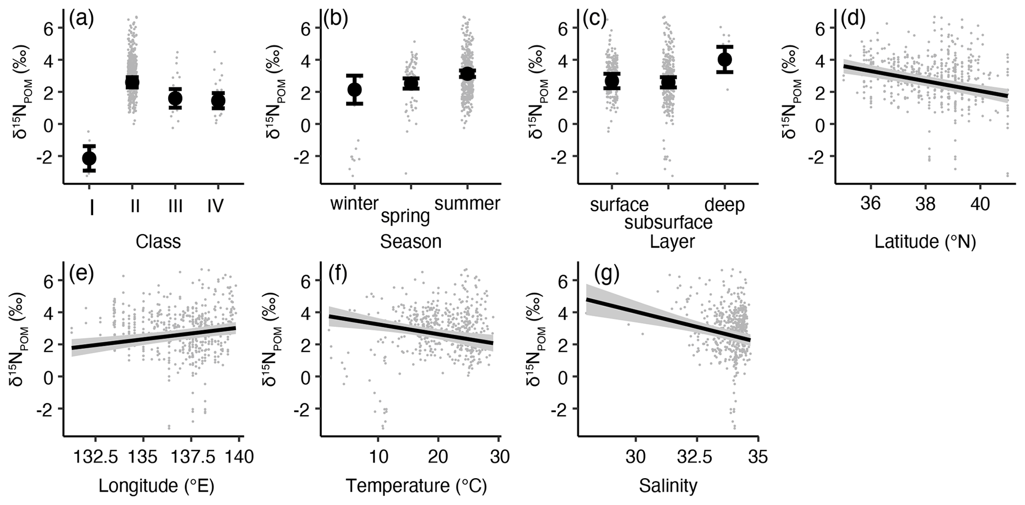
Figure 9Least-square mean (lsmean) values based on the effects of the environmental parameters in the least AIC GLM for δ15NPOM. Effect of (a) classes, (b) sampling seasons, (c) sampling depth, (d) latitude, (e) longitude, (f) temperature, and (g) salinity. Closed circles with bars or solid lines with shadows represent the lsmeans with 95 % confidence intervals. The small gray dots represent the observation data. When necessary, the settings of the class, season, and layer for the calculation of lsmeans were class II, summer, and surface, respectively.
The least AIC δ15NPOM GLM was as follows:
All the parameters were statistically significant (ANOVA, p<0.001), and the r2 value of the model was found to be 0.451. The longitude had a positive impact on δ15NPOM, i.e., δ15NPOM increased eastward (Fig. 9e). The δ15NPOM was negatively affected by the latitude, temperature, and salinity (Fig. 9d, f, g). The lsmean values indicated that the δ15NPOM of classes I (lsmean ± SE: −1.6 ± 0.4 ‰) and II (3.1 ± 0.2 ‰) was significantly lower and higher than those of the other three classes, respectively (pairwise test with Tukey–Kramer adjustment, p<0.01). Moreover, classes III (2.1 ± 0.3 ‰) and IV (2.0 ± 0.3 ‰) were not significantly different (p=0.9735). The seasonal variations exhibited significant differences between spring (1.3 ± 0.2 ‰) and summer (1.9 ± 0.2 ‰, pairwise test with Tukey–Kramer adjustment, p<0.01), while the lowest lsmean values were recorded in winter (0.9 ± 0.4 ‰). No significant differences in lsmean δ15NPOM were found between spring and summer (p>0.0897). The layer indicated that δ15NPOM at a depth of 100 m (2.3 ± 0.4 ‰) was significantly higher (pairwise test with Tukey–Kramer adjustment, p<0.01) than that at the surface (0.9 ± 0.2 ‰) and subsurface (1.0 ± 0.2 ‰).
This study, for the first time, revealed δ13CPOM and δ15NPOM in a wide area of the southern SOJ. Previous studies on δ13CPOM and δ15NPOM were confined to the coastal areas of the southern SOJ (Antonio et al., 2012; Nakamura et al., 2022) and sinking particles (Nakanishi and Minagawa, 2003). Seasonality was demonstrated by the δ13C and δ15N values of sinking organic particles in the deep layer (>500 m depth) (Nakanishi and Minagawa, 2003). Significant seasonality of δ13CPOM and δ15NPOM was observed at the surface in our study, although the pattern of δ13C differed from that seen by Nakanishi and Minagawa (2003). In Nakanishi and Minagawa (2003), the δ13C of sinking particles increased with the bloom period. However, in our study, the δ13CPOM decreased along the SI-line. By contrast, the seasonality of δ15N in the sinking particles and δ15NPOM was comparable. We were unable to determine why the seasonality of δ13CPOM in our study differed from that of Nakanishi and Minagawa (2003). However, our observations indicated that the δ13CPOM and δ15NPOM values at 100 m depth, below the euphotic layer, were significantly different from those in the euphotic zone (Fig. 2), and monthly variations were not significant below the mixed layer. Thus, the characteristics of the sinking particles in the SOJ may be different from those of POM in the surface layer.
4.1 Variations and the causes of the carbon isotope ratio
According to the GLM approach, environmental characteristics may explain approximately two-thirds of the variations in δ13CPOM. The relationships found in this study are consistent with previous observations. When environmental conditions were ignored, seasonal variation was significant; nevertheless, seasonal variation was not selected as an explanatory variable in the GLM, suggesting that environmental parameters can well explain the seasonality of δ13CPOM. The positive associations observed between temperature or chlorophyll-a concentration and δ13CPOM were similar to those observed in previous ocean and incubation experiments (Fontugne and Duplessy, 1981; Goericke and Fry, 1994; Miller et al., 2013; Savoye et al., 2003). Phytoplankton community growth rates are probably high in the warm water (Sherman et al., 2016), and high chlorophyll-a concentrations are considered to be a consequence of rapid phytoplankton growth. During the rapid growth phase, phytoplankton utilizes more 13CO2 in the water, consequently elevating δ13CPOM (Freeman and Hayes, 1992). In addition, the C : N ratio was not selected in the GLM but had a positive relationship with δ13CPOM (Fig. S1). Tanioka and Matsumoto (2020) reported that C : N ratio is elevated with the increase in light based on a meta-analysis, supporting the idea that the active photosynthesis elevates both C : N ratio and δ13CPOM.
The negative relationship between δ13CPOM and salinity or nitrate concentration has been previously reported in the Kuroshio and western North Pacific boundary currents (Kodama et al., 2021). The negative relationship between δ13CPOM and salinity in the Kuroshio area was considered to be a mixture of POM formed in the estuary (Kodama et al., 2021), where phytoplankton bloom occurs and then high-δ13CPOM POM is formed (Savoye et al., 2003; Ogawa and Ogura, 1997). Although our samples were occasionally obtained near the Japanese coast, the less saline water of this sea is mostly due to the influence of the ECS (Kosugi et al., 2021). In the ECS, δ13CPOM is negatively associated with salinity (Ho et al., 2021), and high δ13CPOM (> −20 ‰) is detected in the Changjiang diluted waters due to the sediment resuspension in the Changjiang Estuary (Gao et al., 2014), while the relationship between salinity and δ13CPOM was unknown in Gao et al. (2014) because they did not report the hydrographic characteristics in the high-δ13CPOM area. These facts indicated that the negative relationship between δ13CPOM and salinity pointed to the importance and impact of the processes at the Changjiang Estuary in the SOJ. The direct influence of terrestrial organic matter from China may be ignored: the δ13CPOM in the Changjiang is < −25 ‰ (Gao et al., 2014), while the contribution of terrestrial organic matter is <10 % 500 km away from the Changjiang Estuary (Wu et al., 2003). The effects of Japanese local rivers cannot be ignored, where river-originating δ13CPOM is ∼ −24 ‰ and lower than the ocean-originating δ13CPOM (Antonio et al., 2012), and thus, the direct influence of terrestrial organic matter is deemed to be restricted in the SOJ based on the relationship between salinity and δ13CPOM. These results suggest that POM with high δ13CPOM from the less saline waters of the ECS is transported into the SOJ and influences the spatiotemporal variation in δ13CPOM in the SOJ, particularly during the summer, when the Changjiang-origin freshwater inputs to the SOJ via the Tsushima Strait are the highest among the seasons (Morimoto et al., 2009). We could not come up with a plausible explanation for the negative relationship between latitude and nitrate concentration.
The environmental parameters properly explained δ13CPOM variability but not the difference among classes (III and IV) because it was significant in the GLM. Temperature, nitrate concentration, and C : N ratio were found to be significantly different across classes III and IV. The high δ13CPOM with a low nitrate concentration and high C : N ratio in the class IV samples may be attributed to active carbon assimilation under nitrate depletion conditions, while the chlorophyll a concentration was low in the class IV samples. In contrast to class IV samples, low-δ13CPOM samples in class III were mostly observed in nitrate-rich waters, indicating that primary production is not active due to light limitation induced by the deep mixing and sampling below the light-compensation depth; the previous study's iron limitation for primary production was rejected (Fujita et al., 2010). Liu et al. (2007) reported that low δ13CPOM is observed at the subsurface layer in the South China Sea due to low growth rate, which corresponds to our results. However, comparable environmental conditions of class III and IV samples were observed in the class I and II samples, and hence the fundamental reason why the δ13CPOM was low and high in classes III and IV, respectively, is as yet unclear. According to the T-S diagram, class IV POM was in the warm and saline waters in 2019. This may indicate that the isotope fraction in this water is different; for example, an increase in diatom abundance elevates δ13CPOM (Lowe et al., 2014), but the diatom contribution in the SOJ is low during the summer (Kodama et al., 2022b). The phytoplankton community structure was not assessed in this study and will need to be investigated more in the future.
4.2 Unique nitrogen dynamics in the SOJ
Unlike δ13CPOM, δ15NPOM was not adequately explained by environmental parameters based on the detection coefficient values. Temperature and salinity remained as explanatory variables in the variation in δ15NPOM in the ocean but were not regarded as essential determinants (Sigman et al., 2009). Temperature had the opposite impact as reported in the Kuroshio (Kodama et al., 2021). Temperature had no significant effect in the southwestern ECS (Ho et al., 2021), thereby suggesting that the negative impact of temperature on the δ15NPOM was specific to the SOJ; however, its mechanisms remain unclear.
The negative impact of salinity was similar to that observed in the Kuroshio (Kodama et al., 2021). In June 2010, the δ15NPOM in the surface, less saline Changjiang diluted water (at 5 m depth and salinity <30) was recorded to be ∼ 9 ‰ in the northern part of the ECS (Sukigara et al., 2017). In 2011, the δ15NPOM in the Changjiang diluted water in 2011 was ∼ 6 ‰ (Sukigara et al., 2017). Sukigara et al. (2017) stated that POM with high δ15NPOM was not always present in the Changjiang diluted water, although high δ15NPOM was also reported in the ECS in previous studies (Gao et al., 2014; Wu et al., 2003). These findings corroborate the hypothesis that high δ15NPOM levels originate from the less saline Changjiang diluted water, which mainly flows into the SOJ during the summer (Morimoto et al., 2009), and from the negative relationship between salinity and δ15NPOM.
There are two proposed mechanisms for the influence of latitude on the δ15NPOM. One is the Japanese territorial influence. The other is the impact of the coastal branch of the Tsushima Warm Current. The coastal branch of the Tsushima Warm Current originates from the eastern channel of the Tsushima Strait and flows along the Japanese coast (Katoh, 1994). Our monitoring regions always included a coastal region in the low-latitude area as well as flows of the coastal branch of the Tsushima Warm Current (Katoh, 1994). The δ13CPOM did not indicate direct territorial inputs in this case; thus the influence of the coastal branch of the Tsushima Warm Current and the origin of the waters may be the explanation.
Although ocean observations indicated a negative relationship between δ15NPOM and nitrate concentration based on Rayleigh fractionation (Kodama et al., 2021; Ho et al., 2021), the negative relationship in the SOJ remained equivocal. Even in an open system, kinetic isotope effects (δ15N difference between reactant and product) and the degree of consumption of the reactant theoretically determine the δ15N value of the product, and when the remaining reactant is zero (i.e., completely consumed), the δ15N of a product is equal to the original δ15N of the reactant (Sigman et al., 2009). In this case, the kinetic isotope effect of nitrate on POM is ∼ 3 ‰ (Sigman et al., 2009). Thus, δ15NPOM is theoretically 0 ‰–3 ‰ lower than δ15N of nitrate (δ15N), and with nitrate consumption, it increases and approaches the original δ15N value. The monthly variations in the surface layer along the SI-line indicated that the δ15NPOM increases from winter to summer, and the GLM method confirms this trend. This also indicates that nitrate depletion partly contributes to the increase in δ15NPOM. Because δ15NPOM was not normally distributed, the association was insignificant (p=0.4467) when we removed class I POM, indicating that the relationships between δ15NPOM and the environment, especially the nitrate concentration in the SOJ, were unique.
The following are two possible reasons for the ambiguous relationship between δ15NPOM and nitrate concentration: (1) the nature of our dataset and (2) the variety of nitrogen sources. First, our observations were mainly conducted in the summer, during which time the nitrate was depleted at the surface, and the nitrate concentration in 182 of the 494 samples was not detectable (<0.01 µM). The δ15NPOM in the nitrate-depleted waters varied greatly (mean ± SD: 2.8 ± 1.2 ‰; n=182). This δ15NPOM variation in nitrate-depleted water may have rendered the relationship between δ15NPOM and nitrate concentration unclear, rendering the association statistically insignificant. When the GLM approach was conducted for subsamples with detectable nitrate (>0.01 µM), the nitrate concentration remained as the explanatory variable in the least AIC model; the coefficient was negative but not significant (ANOVA, p=0.12). As a result, the imbalanced dataset was not rejected; nonetheless, it was not the primary cause of the ambiguous relationship between δ15NPOM and nitrate concentration.
Second, the nitrogenous (nitrate) source of the SOJ exhibited variability. Previous studies in the northern ECS (Umezawa et al., 2014, 2021) found four nitrate sources with varying δ15N. The nitrate with high δ15N (8.3 ‰) originated from the Changjiang freshwater in July, the nitrate with low δ15N (2.0 ‰) originated from the Changjiang Estuary in July, the δ15N in the water originating from the Kuroshio is 5.5 ‰–6.0 ‰ in February, and that originating from atmospheric deposition is −4 ‰ to 0 ‰ (Umezawa et al., 2014, 2021). Furthermore, active nitrogen fixation occurs in the northwestern ECS (Shiozaki et al., 2010), and δ15NPOM originating from nitrogen fixation is −2.1 ‰ to 0.8 ‰ (Minagawa and Wada, 1986). According to these results, the δ15NPOM formed by nitrate assimilation and nitrogen fixation exhibited a wider range. In fact, in the ECS, where the TWC originates, δ15NPOM near the surface varies widely from about −5 ‰ to 9 ‰ during summer (Gao et al., 2014) and 2 ‰–6 ‰ in autumn (Wu et al., 2003). Horizontal advective transport of nitrate from the ECS is the key factor for controlling primary production in the SOJ throughout the summer (Kodama et al., 2015, 2017). POM originating from diverse nitrogenous sources will be mixed during the horizontal advection processes in the TWC and the ECS, and POM from the ECS is expected to flow into the SOJ with nitrate. The numerous nitrogen source contributions would obscure the δ15NPOM and nitrate concentration in the SOJ.
Here, a simulation of the relationship between the δ15NPOM and nitrate concentration was performed (see the Supplement). The δ15N was set to 0 ‰–8.3 ‰ (Umezawa et al., 2014, 2021), the kinetic isotope effect of nitrate assimilation to 3 ‰ (Sigman et al., 2009), and the initially supplied nitrate concentration to 0.05–10 µM. The δ15NPOM was then calculated by mixing nitrate-origin POM and nitrogen-fixation-origin POM. Based on observations in the southern ECS in summer, the contribution of nitrogen fixation to nitrate assimilation in the water column was reported as 10 %–82 % (Liu et al., 2013). δ15NPOM produced with nitrogen fixation was set to range from −2.1 ‰ to 0.8 ‰ (Minagawa and Wada, 1986). The fraction of remanent nitrate was set to 0 %–50 %. Then δ15NPOM was calculated based on Sigman et al. (2009), with the random values in the setting ranges except for the kinetic isotope effect. The sample size was set to 500, and the relationship between δ15NPOM and remnant nitrate concentration was evaluated. When this comparison was conducted 1000 times, the insignificant relationship between the δ15NPOM and nitrate concentration was observed in ∼ 70 % of the simulations (Fig. S2). On the other hand, when the δ15N was adjusted to 5 ‰–6 ‰, the significant negative relationship between δ15NPOM and nitrate concentration was consistently observed (Fig. S2). This result supports our hypothesis that the relationship between the δ15NPOM and nitrate concentration is disrupted by the numerous nitrogen sources.
Another distinctive feature of the SOJ was the low-δ15NPOM-designated class I, which was found only in the winter, and is characterized in the T-S diagrams. The low-δ15NPOM was mainly observed in temperature and salinity ranges of 9.4–11.4 ∘C and 33.877–34.038, respectively. Wagawa et al. (2020) classified this water as “upper low salinity water” (ULSW). Despite the fact that the origin of ULSW was unclear, Wagawa et al. (2020) proposed that it originated from Toyama Bay, with less saline conditions caused by the mixing with local Japanese rivers. It is reasonable to assume that the ULSW is not mixed with the saline TWC water (its salinity is ∼ 34.5). Because this saline TWC water originates from the Kuroshio Current, the δ15N of the saline TWC water is estimated to be 5.5 ‰–6.0 ‰ in accordance with Umezawa et al. (2014). At the same time, the δ15N of local Japanese rivers has been estimated to be 0 ‰–2 ‰ (Sugimoto et al., 2019), suggesting that POM in the ULSW may have originated from lower δ15N nitrate than the Kuroshio-origin nitrate, and hence the δ15NPOM is lower than the other water masses. The horizontal distribution of ULSW is not reported, but we assumed that it was not large and confined to winter and spring based on Wagawa et al. (2020); hence, the low-δ15NPOM area would be limited to season and area. Phytoplankton bloom is another possibility for class I. δ15NPOM rapidly declined at the start of the phytoplankton bloom phase but quickly rose with nitrate depletion (Nakatsuka et al., 1992). The class I samples were collected in February, and the phytoplankton bloom occurred at the end of March (Kodama et al., 2018; Maúre et al., 2017), but the chlorophyll-a concentration was not low in class I, and the C : N ratio (6.05 ± 0.58 mol mol−1) of class I (Fig. 6) did not suggest a strong river-origin POM contribution. Therefore, the effects of phytoplankton bloom could not be rejected.
Seasonality remained significant after accounting for hydrographic conditions in the GLM. Not only nitrate concentrations but also nitrogen sources have a seasonality in the SOJ. The mixed layer deepens in the winter, and hence the nitrate originated in deep-sea water or local Japanese rivers in this season. The utilization of nitrate provided in winter occurs in spring, and the Tsushima Warm Current remains weak (Yabe et al., 2021). Kodama et al. (2015) also showed that a subsurface nutrient maximum induced by the horizontal advective transport of the Tsushima Warm Current could be observed from the beginning of June. Therefore, the seasonality of δ15NPOM may be associated with horizontal advective transport, although additional research is required to understand the seasonality.
In this study, the δ13CPOM and δ15NPOM values in the southern SOJ were investigated and reported for the first time. Our observations were mostly conducted in the summer; therefore our identified characteristics of δ13CPOM and δ15NPOM mainly reflected the characteristics of the summer in the SOJ, while seasonality, except autumn, was covered by the monitoring line. There were significant seasonal variations in δ13CPOM and δ15NPOM in the surface mixed layer but not below the mixed layer (at 30 m depth). Environmental variables and primary production processes adequately explained the observed δ13CPOM value. δ13CPOM could be estimated using our GLM and routine hydrographic observations. However, environmental variables did not adequately explain the variation in δ15NPOM. In particular, the relationship between nitrate concentrations was not found. The SOJ contains different nitrogenous sources, such as atmospheric depositions and riverine inputs, and δ15NPOM indicates that these sources are mixed and support primary production. The simulation supported the idea that multiple nitrate sources contributed to the ambiguous relationship between δ15NPOM and nitrate concentration. The main nitrogen source in the SOJ was not detected in our study, but the new production was dependent on the nitrate supplied from these sources. Anthropogenic nitrogen inputs were increased in the SOJ (Duan et al., 2007; Kitayama et al., 2012), and, hence, the anthropogenic-nitrogen-induced production in the SOJ is expected to increase. As a result, we must evaluate the impact of “increased” production on the biogeochemical cycles and ecosystems in the SOJ.
The stable isotope ratio of POM with environmental data used for the statistical analysis in the study is available at PANGAEA (https://doi.org/10.1594/PANGAEA.949287, Kodama et al., 2022c).
The supplement related to this article is available online at: https://doi.org/10.5194/bg-20-3667-2023-supplement.
TK and KN designed the experiments. All authors carried them out. TK and AN prepared the paper with contributions from all co-authors.
The contact author has declared that none of the authors has any competing interests.
Publisher’s note: Copernicus Publications remains neutral with regard to jurisdictional claims in published maps and institutional affiliations.
We would like to thank the captains, crews, researchers, and staff who took part in the cruises. In particular, we would like to thank Keiko Yamada for her assistance with the stable isotope analysis. We state that there is no conflict of interest, and the Japanese government granted authorization for all of observations in accordance with Japanese legislation.
This research has been supported by the Japan Society for the Promotion of Science (grant no. 19K06198, 22K03729, and 23H02285), the Japan Fisheries Research and Education Agency, and the Fisheries Agency.
This paper was edited by Koji Suzuki and reviewed by two anonymous referees.
Antonio, E. S., Kasai, A., Ueno, M., Ishihi, Y., Yokoyama, H., and Yamashita, Y.: Spatial-temporal feeding dynamics of benthic communities in an estuary-marine gradient, Estuar. Coast. Shelf S., 112, 86–97, https://doi.org/10.1016/j.ecss.2011.11.017, 2012.
Buchanan, P. J., Matear, R. J., Chase, Z., Phipps, S. J., and Bindoff, N. L.: Ocean carbon and nitrogen isotopes in CSIRO Mk3L-COAL version 1.0: a tool for palaeoceanographic research, Geosci. Model Dev., 12, 1491–1523, https://doi.org/10.5194/gmd-12-1491-2019, 2019.
Duan, S. W., Xu, F., and Wang, L. J.: Long-term changes in nutrient concentrations of the Changjiang River and principal tributaries, Biogeochemistry, 85, 215–234, https://doi.org/10.1007/s10533-007-9130-2, 2007.
Fontugne, M. and Duplessy, J.: Organic-carbon isotopic fractionation by marine plankton in the temperature range −1 to 31 ∘C, Oceanol. Acta, 4, 85–90, 1981.
Fox, J. and Weisberg, S.: An R companion to applied regression, Sage publications, 2018.
Freeman, K. H. and Hayes, J. M.: Fractionation of carbon isotopes by phytoplankton and estimates of ancient CO2 levels, Global Biogeochem. Cy., 6, 185–198, https://doi.org/10.1029/92GB00190, 1992.
Fujita, S., Kuma, K., Ishikawa, S., Nishimura, S., Nakayama, Y., Ushizaka, S., Isoda, Y., Otosaka, S., and Aramaki, T.: Iron distributions in the water column of the Japan Basin and Yamato Basin (Japan Sea), J. Geophys. Res.-Oceans, 115, C12001, https://doi.org/10.1029/2010JC006123, 2010.
Gao, L., Li, D., and Ishizaka, J.: Stable isotope ratios of carbon and nitrogen in suspended organic matter: Seasonal and spatial dynamics along the Changjiang (Yangtze River) transport pathway, J. Geophys. Res.-Biogeo., 119, 1717–1737, https://doi.org/10.1002/2013JG002487, 2014.
Goericke, R. and Fry, B.: Variations of marine plankton δ13C with latitude, temperature, and dissolved CO2 in the world ocean, Global Biogeochem. Cy., 8, 85–90, https://doi.org/10.1029/93gb03272, 1994.
Gruber, N. and Galloway, J. N.: An Earth-system perspective of the global nitrogen cycle, Nature, 451, 293–296, https://doi.org/10.1038/nature06592, 2008.
Gruber, N., Keeling, C. D., Bacastow, R. B., Guenther, P. R., Lueker, T. J., Wahlen, M., Meijer, H. A. J., Mook, W. G., and Stocker, T. F.: Spatiotemporal patterns of carbon-13 in the global surface oceans and the oceanic suess effect, Global Biogeochem. Cy., 13, 307–335, https://doi.org/10.1029/1999gb900019, 1999.
Guo, X., Miyazawa, Y., and Yamagata, T.: The Kuroshio onshore intrusion along the shelf break of the East China Sea: the origin of the Tsushima Warm Current, J. Phys. Oceanogr., 36, 2205–2231, https://doi.org/10.1175/jpo2976.1, 2006.
Hashimoto, R., Yoshida, T., Kuno, S., Nishikawa, T., and Sako, Y.: The first assessment of cyanobacterial and diazotrophic diversities in the Japan Sea, Fish. Sci., 78, 1293–1300, https://doi.org/10.1007/s12562-012-0548-7, 2012.
Ho, P.-C., Okuda, N., Yeh, C.-F., Wang, P.-L., Gong, G.-C., and Hsieh, C.-H.: Carbon and nitrogen isoscape of particulate organic matter in the East China Sea, Prog. Oceanogr., 197, 102667, https://doi.org/10.1016/j.pocean.2021.102667, 2021.
Ishizu, M., Miyazawa, Y., Tsunoda, T., and Ono, T.: Long-term trends in pH in Japanese coastal seawater, Biogeosciences, 16, 4747–4763, https://doi.org/10.5194/bg-16-4747-2019, 2019.
Isobe, A.: On the origin of the Tsushima Warm Current and its seasonality, Cont. Shelf Res., 19, 117–133, https://doi.org/10.1016/s0278-4343(98)00065-x, 1999.
Katoh, O.: Structure of the Tsushima Current in the southwestern Japan Sea, J. Oceanogr., 50, 317–338, 1994.
Kim, S. K., Chang, K. I., Kim, B., and Cho, Y. K.: Contribution of ocean current to the increase in N abundance in the Northwestern Pacific marginal seas, Geophys. Res. Lett., 40, 143–148, https://doi.org/10.1029/2012GL054545, 2013.
Kim, T. W., Lee, K., Najjar, R. G., Jeong, H. D., and Jeong, H. J.: Increasing N abundance in the northwestern Pacific Ocean due to atmospheric nitrogen deposition, Science, 334, 505–509, https://doi.org/10.1126/science.1206583, 2011.
Kitayama, K., Seto, S., Sato, M., and Hara, H.: Increases of wet deposition at remote sites in Japan from 1991 to 2009, J. Atmos. Chem., 69, 33–46, https://doi.org/10.1007/s10874-012-9228-3, 2012.
Kodama, T.: The nutrient dynamics and the lower trophic ecosystems in the warm waters in the vicinity of Japan, Oceanography in Japan, 29, 55–69, https://doi.org/10.5928/kaiyou.29.2_55, 2020.
Kodama, T., Morimoto, H., Igeta, Y., and Ichikawa, T.: Macroscale-wide nutrient inversions in the subsurface layer of the Japan Sea during summer, J. Geophys. Res., 120, 7476–7492, https://doi.org/10.1002/2015jc010845, 2015.
Kodama, T., Igeta, Y., Kuga, M., and Abe, S.: Long-term decrease in phosphate concentrations in the surface layer of the southern Japan Sea, J. Geophys. Res., 121, 7845–7856, https://doi.org/10.1002/2016jc012168, 2016.
Kodama, T., Morimoto, A., Takikawa, T., Ito, M., Igeta, Y., Abe, S., Fukudome, K., Honda, N., and Katoh, O.: Presence of high nitrate to phosphate ratio subsurface water in the Tsushima Strait during summer, J. Oceanogr., 73, 759–769, https://doi.org/10.1007/s10872-017-0430-4, 2017.
Kodama, T., Wagawa, T., Ohshimo, S., Morimoto, H., Iguchi, N., Fukudome, K. I., Goto, T., Takahashi, M., and Yasuda, T.: Improvement in recruitment of Japanese sardine with delays of the spring phytoplankton bloom in the Sea of Japan, Fish. Oceanogr., 27, 289–301, https://doi.org/10.1111/fog.12252, 2018.
Kodama, T., Nishimoto, A., Horii, S., Ito, D., Yamaguchi, T., Hidaka, K., Setou, T., and Ono, T.: Spatial and seasonal variations of stable isotope ratios of particulate organic carbon and nitrogen in the surface water of the Kuroshio, J. Geophys. Res., 126, e2021JC017175, https://doi.org/10.1029/2021JC017175, 2021.
Kodama, T., Igeta, Y., and Iguchi, N.: Long-term variation in mesozooplankton biomass caused by top-down effects: a case study in the coastal Sea of Japan, Geophys. Res. Lett., 49, e2022GL099037, https://doi.org/10.1029/2022gl099037, 2022a.
Kodama, T., Taniuchi, Y., Kasai, H., Yamaguchi, T., Nakae, M., and Okumura, Y.: Empirical estimation of marine phytoplankton assemblages in coastal and offshore areas using an in situ multi-wavelength excitation fluorometer, Plos One, 17, e0257258, https://doi.org/10.1371/journal.pone.0257258, 2022b.
Kodama, T., Nishimoto, A., Nakamura, K., Nakae, M., Iguchi, N., Igeta, Y., and Kogure, Y.: Carbon and nitrogen stable isotope ratios of particulate organic matter in the southern Sea of Japan from 2018 to 2021, PANGAEA [data set], https://doi.org/10.1594/PANGAEA.949287, 2022c.
Kosugi, N., Sasano, D., Ishii, M., Enyo, K., and Saito, S.: Autumn CO2 chemistry in the Japan Sea and the impact of discharges from the Changjiang River, J. Geophys. Res., 121, 6536–6549, https://doi.org/10.1002/2016jc011838, 2016.
Kosugi, N., Hirose, N., Toyoda, T., and Ishii, M.: Rapid freshening of Japan Sea Intermediate Water in the 2010s, J. Oceanogr., 77, 269–281, https://doi.org/10.1007/s10872-020-00570-6, 2021.
Liu, K.-K., Kao, S.-J., Hu, H.-C., Chou, W.-C., Hung, G.-W., and Tseng, C.-M.: Carbon isotopic composition of suspended and sinking particulate organic matter in the northern South China Sea – From production to deposition, Deep-Sea Res. Pt. II, 54, 1504–1527, https://doi.org/10.1016/j.dsr2.2007.05.010, 2007.
Liu, X., Furuya, K., Shiozaki, T., Masuda, T., Kodama, T., Sato, M., Kaneko, H., Nagasawa, M., and Yasuda, I.: Variability in nitrogen sources for new production in the vicinity of the shelf edge of the East China Sea in summer, Cont. Shelf Res., 61–62, 23–30, https://doi.org/10.1016/j.csr.2013.04.014, 2013.
Lorrain, A., Savoye, N., Chauvaud, L., Paulet, Y.-M., and Naulet, N.: Decarbonation and preservation method for the analysis of organic C and N contents and stable isotope ratios of low-carbonated suspended particulate material, Anal. Chim. Acta, 491, 125–133, https://doi.org/10.1016/S0003-2670(03)00815-8, 2003.
Lorrain, A., Pethybridge, H., Cassar, N., Receveur, A., Allain, V., Bodin, N., Bopp, L., Choy, C. A., Duffy, L., Fry, B., Goni, N., Graham, B. S., Hobday, A. J., Logan, J. M., Menard, F., Menkes, C. E., Olson, R. J., Pagendam, D. E., Point, D., Revill, A. T., Somes, C. J., and Young, J. W.: Trends in tuna carbon isotopes suggest global changes in pelagic phytoplankton communities, Glob. Change Biol., 26, 458–470, https://doi.org/10.1111/gcb.14858, 2020.
Lowe, A. T., Galloway, A. W. E., Yeung, J. S., Dethier, M. N., and Duggins, D. O.: Broad sampling and diverse biomarkers allow characterization of nearshore particulate organic matter, Oikos, 123, 1341–1354, https://doi.org/10.1111/oik.01392, 2014.
Lüdecke, D.: ggeffects: Tidy data frames of marginal effects from regression models, Journal of Open Source Software, 3, 772, https://doi.org/10.21105/joss.00772, 2018.
Maúre, E. R., Ishizaka, J., Sukigara, C., Mino, Y., Aiki, H., Matsuno, T., Tomita, H., Goes, J. I., and Gomes, H. R.: Mesoscale eddies control the timing of spring phytoplankton blooms: A case study in the Japan Sea, Geophys. Res. Lett., 44, 11115–11124, https://doi.org/10.1002/2017GL074359, 2017.
Miller, R. J., Page, H. M., and Brzezinski, M. A.: δ13C and δ15N of particulate organic matter in the Santa Barbara Channel: drivers and implications for trophic inference, Mar. Ecol.-Prog. Ser., 474, 53–66, https://doi.org/10.3354/meps10098, 2013.
Minagawa, M. and Wada, E.: Nitrogen isotope ratios of red tide organisms in the East China Sea: A characterization of biological nitrogen fixation, Mar. Chem., 19, 245–259, https://doi.org/10.1016/0304-4203(86)90026-5, 1986.
Morimoto, A., Takikawa, T., Onitsuka, G., Watanabe, A., Moku, M., and Yanagi, T.: Seasonal variation of horizontal material transport through the eastern channel of the Tsushima Straits, J. Oceanogr., 65, 61–71, https://doi.org/10.1007/s10872-009-0006-z, 2009.
Nakamura, K., Nishimoto, A., Yasui-Tamura, S., Kogure, Y., Nakae, M., Iguchi, N., Morimoto, H., and Kodama, T.: Carbon and nitrogen dynamics in the coastal Sea of Japan inferred from 15 years of measurements of stable isotope ratios of Calanus sinicus, Ocean Sci., 18, 295–305, https://doi.org/10.5194/os-18-295-2022, 2022.
Nakanishi, T. and Minagawa, M.: Stable carbon and nitrogen isotopic compositions of sinking particles in the northeast Japan Sea, Geochem. J., 37, 261–275, https://doi.org/10.2343/geochemj.37.261, 2003.
Nakatsuka, T., Handa, N., Wada, E., and Wong, C. S.: The dynamic changes of stable isotopic ratios of carbon and nitrogen in suspended and sedimented particulate organic matter during a phytoplankton bloom, J. Mar. Res., 50, 267–296, https://elischolar.library.yale.edu/journal_of_marine_research/2035 (last access: 9 September 2023), 1992.
Ogawa, N. and Ogura, N.: Dynamics of particulate organic matter in the Tamagawa estuary and inner Tokyo Bay, Estuar. Coast. Shelf S., 44, 263–273, https://doi.org/10.1006/ecss.1996.0118, 1997.
Ohishi, S., Aiki, H., Tozuka, T., and Cronin, M. F.: Frontolysis by surface heat flux in the eastern Japan Sea: importance of mixed layer depth, J. Oceanogr., 75, 283–297, https://doi.org/10.1007/s10872-018-0502-0, 2019.
Ohshimo, S., Kodama, T., Yasuda, T., Kitajima, S., Tsuji, T., Kidokoro, H., and Tanaka, H.: Potential fluctuation of δ13C and δ15N values of small pelagic forage fish in the Sea of Japan and East China Sea, Mar. Freshwater Res., 72, 1811, https://doi.org/10.1071/mf20351, 2021.
Omstedt, A.: How to develop an understanding of the marginal sea system by connecting natural and human sciences, Oceanologia, 61, 20–29, https://doi.org/10.1016/j.oceano.2021.06.003, 2021.
Ono, T.: Long-term trends of oxygen concentration in the waters in bank and shelves of the Southern Japan Sea, J. Oceanogr., 77, 659–684, https://doi.org/10.1007/s10872-021-00599-1, 2021.
R Core Team: R: A language and environment for statistical computing, R Foundation for Statistical Computing [code], https://www.R-project.org/ (last access: 9 September 2023), 2023.
Ren, H., Chen, Y. C., Wang, X. T., Wong, G. T. F., Cohen, A. L., DeCarlo, T. M., Weigand, M. A., Mii, H. S., and Sigman, D. M.: 21st-century rise in anthropogenic nitrogen deposition on a remote coral reef, Science, 356, 749–752, doi10.1126/science.aal3869, 2017.
Sato, R., Kawanishi, H., Schimmelmann, A., Suzuki, Y., and Chikaraishi, Y.: New amino acid reference materials for stable nitrogen isotope analysis, BUNSEKI KAGAKU, 63, 399–403, https://doi.org/10.2116/bunsekikagaku.63.399, 2014 (in Japanese with English abstract).
Sato, T., Shiozaki, T., Taniuchi, Y., Kasai, H., and Takahashi, K.: Nitrogen fixation and diazotroph community in the subarctic Sea of Japan and Sea of Okhotsk, J. Geophys. Res.-Oceans, 126, e2020JC017071, https://doi.org/10.1029/2020jc017071, 2021.
Savoye, N., Aminot, A., Tréguer, P., Fontugne, M., Naulet, N., and Kérouel, R.: Dynamics of particulate organic matter δ15N and δ13C during spring phytoplankton blooms in a macrotidal ecosystem (Bay of Seine, France), Mar. Ecol.-Prog. Ser., 255, 27–41, https://doi.org/10.3354/meps255027, 2003.
Scrucca, L., Fop, M., Murphy, T. B., and Raftery, A. E.: mclust 5: Clustering, classification and density estimation using Gaussian finite mixture models, R J., 8, 289–317, https://doi.org/10.32614/RJ-2016-021, 2016.
Sherman, E., Moore, J. K., Primeau, F., and Tanouye, D.: Temperature influence on phytoplankton community growth rates, Global Biogeochem. Cy., 30, 550–559, https://doi.org/10.1002/2015gb005272, 2016.
Shiozaki, T., Furuya, K., Kodama, T., Kitajima, S., Takeda, S., Takemura, T., and Kanda, J.: New estimation of N2 fixation in the western and central Pacific Ocean and its marginal seas, Global Biogeochem. Cy., 24, GB1015, https://doi.org/10.1029/2009gb003620, 2010.
Sigman, D. M., Karsh, K. L., and Casciotti, K. L.: Nitrogen isotopes in the ocean, in: Encyclopedia of Ocean Sciences, edited by: Steele, J. H., Academic Press, Oxford, 40–54, https://doi.org/10.1016/b978-012374473-9.00632-9, 2009.
Sugimoto, R., Tsuboi, T., and Fujita, M. S.: Comprehensive and quantitative assessment of nitrate dynamics in two contrasting forested basins along the Sea of Japan using dual isotopes of nitrate, Sci. Total Environ., 687, 667–678, https://doi.org/10.1016/j.scitotenv.2019.06.090, 2019.
Sukigara, C., Mino, Y., Tripathy, S. C., Ishizaka, J., and Matsuno, T.: Impacts of the Changjiang diluted water on sinking processes of particulate organic matters in the East China Sea, Cont. Shelf Res., 151, 84–93, https://doi.org/10.1016/j.csr.2017.10.012, 2017.
Tanioka, T. and Matsumoto, K.: A meta-analysis on environmental drivers of marine phytoplankton C : N : P, Biogeosciences, 17, 2939–2954, https://doi.org/10.5194/bg-17-2939-2020, 2020.
Umezawa, Y., Yamaguchi, A., Ishizaka, J., Hasegawa, T., Yoshimizu, C., Tayasu, I., Yoshimura, H., Morii, Y., Aoshima, T., and Yamawaki, N.: Seasonal shifts in the contributions of the Changjiang River and the Kuroshio Current to nitrate dynamics in the continental shelf of the northern East China Sea based on a nitrate dual isotopic composition approach, Biogeosciences, 11, 1297–1317, https://doi.org/10.5194/bg-11-1297-2014, 2014.
Umezawa, Y., Toyoshima, K., Saitoh, Y., Takeda, S., Tamura, K., Tamaya, C., Yamaguchi, A., Yoshimizu, C., Tayasu, I., and Kawamoto, K.: Evaluation of origin-depended nitrogen input through atmospheric deposition and its effect on primary production in coastal areas of western Kyusyu, Japan, Environ. Pollut., 291, 118034, https://doi.org/10.1016/j.envpol.2021.118034, 2021.
Wagawa, T., Kawaguchi, Y., Igeta, Y., Honda, N., Okunishi, T., and Yabe, I.: Observations of oceanic fronts and water-mass properties in the central Japan Sea: Repeated surveys from an underwater glider, J. Marine Syst., 201, 103242, https://doi.org/10.1016/j.jmarsys.2019.103242, 2020.
Wu, Y., Zhang, J., Li, D. J., Wei, H., and Lu, R. X.: Isotope variability of particulate organic matter at the PN section in the East China Sea, Biogeochemistry, 65, 31–49, https://doi.org/10.1023/a:1026044324643, 2003.
Yabe, I., Kawaguchi, Y., Wagawa, T., and Fujio, S.: Anatomical study of Tsushima Warm Current system: Determination of Principal Pathways and its Variation, Prog. Oceanogr., 194, 102590, https://doi.org/10.1016/j.pocean.2021.102590, 2021.