the Creative Commons Attribution 4.0 License.
the Creative Commons Attribution 4.0 License.
 | 27 Sep 2023
Estimating marine carbon uptake in the northeast Pacific using a neural network approach
Roberta C. Hamme
Debby Ianson
Peter Landschützer
Mohamed M. M. Ahmed
Neil C. Swart
Paul A. Covert
The global ocean takes up nearly a quarter of anthropogenic CO2 emissions annually, but the variability in this uptake at regional scales remains poorly understood. Here we use a neural network approach to interpolate sparse observations, creating a monthly gridded seawater partial pressure of CO2 (pCO2) data product from January 1998 to December 2019, at ∘ × ∘ spatial resolution, in the northeast Pacific open ocean, a net sink region. The data product (ANN-NEP; NCEI Accession 0277836) was created from pCO2 observations within the 2021 version of the Surface Ocean CO2 Atlas (SOCAT) and a range of predictor variables acting as proxies for processes affecting pCO2 to create nonlinear relationships to interpolate observations at a spatial resolution 4 times greater than leading global products and with better overall performance. In moving to a higher resolution, we show that the internal division of training data is the most important parameter for reducing overfitting. Using our pCO2 product, wind speed, and atmospheric CO2, we evaluate air–sea CO2 flux variability. On sub-decadal to decadal timescales, we find that the upwelling strength of the subpolar Alaskan Gyre, driven by large-scale atmospheric forcing, acts as the primary control on air–sea CO2 flux variability (r2=0.93, p<0.01). In the northern part of our study region, divergence from atmospheric CO2 is enhanced by increased local wind stress curl, enhancing upwelling and entrainment of naturally CO2-rich subsurface waters, leading to decade-long intervals of strong winter outgassing. During recent Pacific marine heat waves from 2013 on, we find enhanced atmospheric CO2 uptake (by as much as 45 %) due to limited wintertime entrainment. Our product estimates long-term surface ocean pCO2 increase at a rate below the atmospheric trend (1.4 ± 0.1 µatm yr−1) with the slowest increase in the center of the subpolar gyre where there is strong interaction with subsurface waters. This mismatch suggests the northeast Pacific Ocean sink for atmospheric CO2 may be increasing.
- Article
(6689 KB) - Full-text XML
-
Supplement
(1463 KB) - BibTeX
- EndNote


As countries around the world consider updating their carbon emission reduction commitments (United Nations Environment Programme, 2022), we require a better understanding of global carbon sinks and how they may be shifting under climate change. The global ocean takes up nearly a quarter of anthropogenic carbon dioxide (CO2) emissions annually (Friedlingstein et al., 2022), but the temporal and spatial variability in the marine sink remains unclear on decadal or longer timescales (McKinley et al., 2011; Fay and McKinley, 2013; Wanninkhof et al., 2013; Gruber et al., 2023). Potential future changes in the marine sink associated with climate change are also unclear (O'Neill et al., 2016). Extending the spatial and temporal coverage of the partial pressure of CO2 in seawater (pCO2) observations can help address this knowledge gap (Aricò et al., 2021). Benefitting from the increasing abundance of CO2 measurements at sea and community synthesis efforts (e.g., through the Surface Ocean CO2 Atlas (SOCAT); Bakker et al., 2016), a variety of interpolation approaches have evolved capable of creating continuous observation-based estimates of pCO2 (Denvil-Sommer et al., 2019; Zhong et al., 2022; Laruelle et al., 2017; Nakaoka et al., 2013; Chen et al., 2019; Ritter et al., 2017; Landschützer et al., 2013). However, their global focus and coarse resolution limits their interpretation at regional scales (Olivier et al., 2022). Only recently, higher-resolution regional pCO2 maps have been developed for the California Current System (Sharp et al., 2022) to overcome the limitations of coarse global-scale pCO2 products. These seawater pCO2 products, combined with wind speed and atmospheric pCO2, have informed regional to global air–sea CO2 flux estimates of multiyear variability (Landschützer et al., 2019, 2016, 2015; Wang et al., 2021; Hauck et al., 2020).
No high-resolution observation-based air–sea CO2 flux estimate currently exists for the North Pacific Ocean. The northeast Pacific Ocean has been characterized as a net annual sink for atmospheric CO2 (Wong et al., 2010; Franco et al., 2021; Sutton et al., 2017; Duke et al., 2023b). The region is divided by two dominant oceanographic features: the Alaskan Gyre system to the north and the North Pacific Current to the south (Franco et al., 2021). With respect to surface ocean carbon measurements, the Alaskan Gyre system remains extremely sparsely sampled. The seasonal air–sea CO2 flux of the gyre has been described as being strongly influenced by gyre upwelling with outgassing in the winter and uptake in the summer (Brady et al., 2019; Palevsky et al., 2013; Chierici et al., 2006). Along the easternmost part of the North Pacific Current, most of our understanding comes from a limited region: the Ocean Station Papa mooring at 50∘ N, 145∘ W (Sutton et al., 2017) and the Line P Program (Freeland, 2007). This region has well-documented seasonal cycles (Sutton et al., 2017), interannual variability (Wong and Chan, 1991; Wong et al., 2010), and long-term trends (Franco et al., 2021; Sutton et al., 2019). CO2 uptake is mainly driven by direct ventilation of the shallow upper water column, with a small seasonal change in surface ocean pCO2 (Wong et al., 2010; Sutton et al., 2017). The estimated long-term trend in surface ocean pCO2 appears to be increasing at less than the atmospheric rate of increase (Franco et al., 2021).
Understanding what drives air–sea CO2 fluxes on seasonal, interannual, and decadal timescales in the northeast Pacific Ocean will provide information on how the regional sink may change in the future. This region is already experiencing persistent marine heat waves with dramatic temperature anomalies observed during 2014 to 2016 and 2018 to 2020 events (Freeland and Ross, 2019; Bond et al., 2015), with future events predicted to become longer-lasting, more frequent, more extensive, and more intense (Frölicher et al., 2018). The impact of large-scale climate-driven decadal oscillations on the marine carbon system is just beginning to be explored in models (Hauri et al., 2021). Furthermore, this region has been targeted as a potential site of marine carbon dioxide removal, as a negative emissions technology aimed at meeting emission reduction goals continues to grow in interest and investment (Cooley et al., 2022). Some proposed approaches look to artificially stimulate biological carbon drawdown (GESAMP, 2019; NASEM, 2021). The northeast Pacific Ocean, as an iron-limited high-nutrient low-chlorophyll region (Dugdale and Wilkerson, 1991; Aumont et al., 2003; Martin et al., 1994; Freeland et al., 1984), has already been the location of geoengineered biological carbon drawdown experiments (Boyd et al., 2007, 2005; Wong and Johnson, 2002; Ianson et al., 2012). Thus, a firm understanding of processes driving carbon fluxes and the establishment of environmental baselines in the region is critical.
Our aim is to investigate drivers of air–sea CO2 flux variability in the northeast Pacific (NEP) Ocean, building a novel regional high-resolution artificial neural network (ANN) approach adopted from an existing global setup (Landschützer et al., 2013). In Sect. 2, we describe the creation of a gridded pCO2 data product (herein referred to as ANN-NEP; NCEI Accession 0277836; Duke et al., 2023a) monthly from January 1998 to December 2019 at ∘ × ∘ spatial resolution in the northeast Pacific open ocean (approximately 9 km by 5 km, latitude by longitude). In Sect. 3, we show that the high-resolution regional pCO2 product is robust enough to recreate training observation data while generalizing well compared to independent withheld observation data. We also show that stepping to a higher resolution regionally with appropriate tuning of the internal training and evaluation data ratio does not hinder product performance. In Sect. 4, our results show that the upwelling strength of the subpolar Alaskan Gyre and surface ocean connectivity to subsurface waters act as the primary controls on air–sea CO2 flux variability in our study area. We conclude by calculating long-term trends in surface ocean pCO2 and carbon uptake, examining trends relative to connectivity to subsurface waters.
Our study area comprises the region between latitudes 45 and 62∘ N and longitudes 120 and 155∘ W (Fig. 1), with the open-oceanic and coastal boundary defined as 300 km offshore following Laruelle et al. (2017). We limit our study region to the open-ocean regions with reduced variability and related drivers compared to the continental shelf regions. Creating a product on the continental shelf and in the nearshore areas requires different neural network considerations and is associated with high uncertainties (Laruelle et al., 2017). This work represents a 4-fold increase in spatial resolution over previous multiyear global open-ocean products, usually coarser than ∘ (Landschützer et al., 2020b). The increased resolution derives from high-resolution predictor data used to create the product (Table 1). To interpolate the existing CO2 observations in this domain, we adapt the artificial neural network (ANN) self-organizing-map feed-forward-network (SOM-FFN) approach developed by Landschützer et al. (2013, 2014). In a first step, the method divides the region of interest into dynamic zones with similar biogeochemical features (i.e., SOM biogeochemical provinces), using a self-organizing-map approach. In a second step, a feed-forward neural network is used for interpolating pCO2 observations in each of the pre-determined provinces of step one. Specifically, nonlinear functional relationships are created between pCO2 observations (or neural network target data), where they exist in our study domain, and independent predictor variables (or neural network input data) that are known to drive the marine carbon cycle (see Sect. 2.1 below). Once the relationships are established, they can be applied where no observations exist to fill space and time gaps and create continuous sea surface pCO2 maps from 1998–2019.
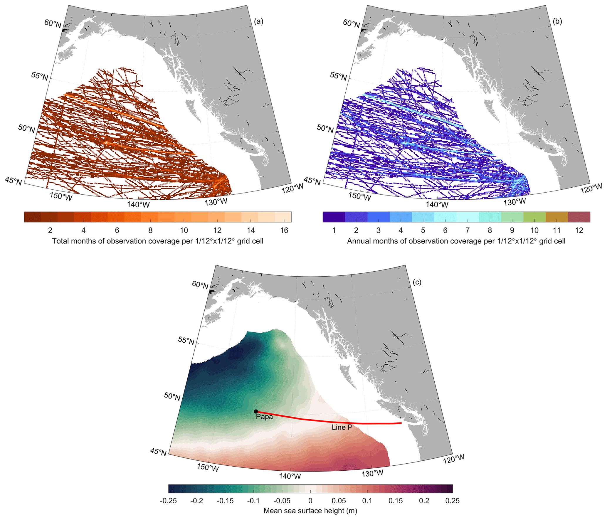
Figure 1(a) Total number of months of observational coverage from Surface Ocean CO2 Atlas (SOCAT) v2021 (Bakker et al., 2016) and additional data from the Fisheries and Oceans Canada February 2019 Line P cruise (https://www.waterproperties.ca/linep/, last access: August 2022) per ∘ × ∘ grid cell. (b) Number of unique annual months of observational coverage per ∘ × ∘ grid cell. (c) Mean sea surface height (SSH; Table 1) shows relative location of the subpolar Alaskan Gyre (negative SSH values) and the North Pacific Current (SSH approximately equal to 0). Ocean Station Papa is labeled and marked with a black circle, while Line P is labeled and marked with a red line.
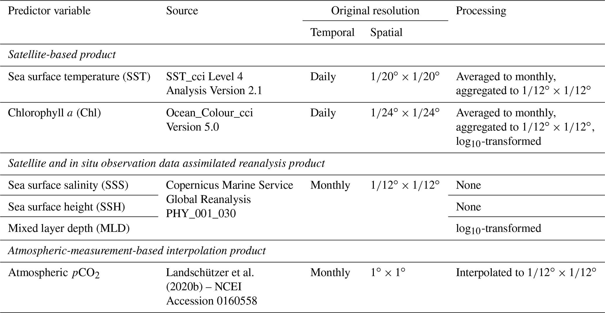
Table 1Northeast Pacific open-ocean artificial neural network predictor variables and their corresponding source, original temporal and spatial resolutions, and processing steps used for this study.
2.1 Predictor data
The chosen predictor variables for this study (Table 1) had all been used previously in observation-based pCO2 interpolated products (Denvil-Sommer et al., 2019; Zhong et al., 2022; Landschützer et al., 2014; Gregor et al., 2018; Telszewski et al., 2009). Sea surface temperature (SST) comes from the satellite-based European Space Agency Climate Change Initiative (Merchant et al., 2019; ESA Sea Surface Temperature Climate Change Initiative (SST_cci): Level 4 Analysis Climate Data Record, version 2.1), as does chlorophyll-a concentration which served as a proxy for biological processes (ESA Ocean Colour Climate Change Initiative, 2022). The remaining physical process predictor data (e.g., sea surface salinity (SSS), sea surface height (SSH), and mixed layer depth (MLD)) are obtained from the Copernicus Marine Environment Monitoring Service global ocean eddy-resolving reanalysis (Global Ocean Physical Reanalysis Product, EU Copernicus Marine Service Information GLOBAL_REANALYSIS_PHY_001_030). Jointly assimilated observations include satellite altimeter data and in situ vertical profiles of temperature and salinity informing the MLD reanalysis product (Table 1). The ocean general circulation model is based on the Nucleus for European Modelling of the Ocean (NEMO) platform, driven at the surface by the European Centre for Medium-Range Weather Forecasts ERA-Interim winds (Jean-Michel et al., 2021). Both chlorophyll a and mixed layer depth were log10-transformed to produce a distribution of values closer to normal before being used in either SOM-FFN step. Atmospheric pCO2 in microatmospheres was downloaded from Landschützer et al. (2020b), derived from the National Oceanic and Atmospheric Administration Earth System Research Global Monitoring Laboratory (https://gml.noaa.gov/ccgg/globalview/, last access: August 2022) atmospheric mole fraction of CO2 (χCO2) and SST (Reynolds et al., 2002) as well as sea level pressure (Kalnay et al., 1996) following Dickson et al. (2007). Finally, the monthly pCO2 climatology of Landschützer et al. (2020a) was used as an additional input parameter solely for defining the SOM biogeochemical provinces.
2.2 pCO2 observations
ANN target pCO2 data come from the Surface Ocean CO2 Atlas (SOCAT) v2021 (Bakker et al., 2016), and there are additional data from the Fisheries and Oceans Canada February 2019 Line P cruise (https://www.waterproperties.ca/linep/, last access: August 2022; Fig. 1c). Sea surface CO2 fugacity (fCO2) was converted to sea surface pCO2 (Text S1 in the Supplement; Körtzinger, 1999). pCO2 observations were bin-averaged into monthly ∘ latitude by ∘ longitude grid cells computing the mean and standard deviation within each grid cell. Of the 8 712 264 grid cells that represent the surface ocean gridded in three dimensions over 264 months (1998–2019) at a ∘ × ∘ resolution in the study area, just 0.39 % have an associated gridded pCO2 value (Fig. 1).
2.3 Evaluation
In constructing the optimal ANN architecture, a series of SOM-FFN tuning tests were conducted comparing ANN output to training and independent withheld data. The ANN performance for each tuning test was evaluated using five statistical metrics: root mean squared error (RMSE), the coefficient of determination (r2), mean absolute error (MAE), mean bias (calculated as the mean residual), and the slope of the linear regression (c1) between the ANN and the corresponding gridded SOCAT pCO2 observations. Independent withheld data came from randomly selected SOCAT data using associated expocodes corresponding to unique complete underway cruise tracks or mooring deployments. We tested 100 random independent withheld data splits and selected one representative of basin-wide observational coverage (summer and southern sampling bias), with winter, spring, and fall data present (Figs. 1 and S1 in the Supplement). These independent withheld data represented approximately 5 % of the total study area gridded pCO2 data, with coverage during all seasons over a range of latitudes (Fig. S1). Ensuring that selected independent withheld data are random yet also representative of the full domain, without withholding critical end range training data, is difficult. Community-based best practices are likely needed going forward to ensure continuity in reported observation-based pCO2 product uncertainty based on independent withheld data (Sect. 3.2).
2.4 Neural network construction
SOM-FFN tuning tests occurred in series using the MATLAB Neural Network Toolbox, with sequential improvements impacting future tests. The optimization of the SOM-derived biogeochemical provinces involved trial-and-error testing of various parameters including SOM biogeochemical province count, predictor variable choice, and static or varying province shape with each time step (Landschützer et al., 2013). The choice of four SOM biogeochemical provinces represented the lowest number of SOM biogeochemical provinces for a typical clustering structure to emerge (Fig. S2), while keeping the ratio of gridded pCO2 observations to the total grid cells within each province similar (0.38 ± 0.06 %). The best SOM predictor variables were SST, SSS, MLD (Table 1), and the Landschützer et al. (2020a) pCO2 climatology. We did not normalize predictor data (e.g., force a mean of 0 and standard deviation of 1), implicitly weighting SOM predictors toward the pCO2 climatology as its range is at least 1 order of magnitude greater than that for SST, SSS, and log(MLD) (Landschützer et al., 2013). As a result, our dynamic provinces follow the seasonal variations in the pCO2 climatology (Landschützer et al., 2020a). Thus, non-static provinces, which changed shape from 1 month to the next over a climatology, proved the most useful in clustering seasonal cycle variability. This clustering does lead to clearly unphysical fronts as an artifact of the approach.
In reaching an optimal FFN architecture (i.e., number of inputs, number of hidden layers and neurons in each hidden layer), trial-and-error testing of tuning parameters explored predictor variable choice, FFN training algorithm and activation functions, pre-training to determine the number of neurons in the first hidden layer, introducing a second hidden layer with a static number of neurons, and changing the internal data division ratio (optimized at 94 : 6; see Sect. 3.4 below).
To emphasize interannual and longer-term trends within the six predictor variables (Table 1), each predictor variable is used in two different forms: first in its raw form and second after de-seasonalizing, bringing the total number of FFN predictors used to 12. To de-seasonalize a variable, within each grid cell, the monthly anomaly was calculated by subtracting the climatological monthly mean, removing the seasonal cycle from the data (the same approach is used when looking at anomaly values in our results; Sect. 4). Where no chlorophyll-a satellite data were available, the ANN was run again with the remaining predictors and output was merged to fill empty grid cells (Landschützer et al., 2014). The Levenberg–Marquardt backpropagation training algorithm and hyperbolic tangent sigmoid activation function (i.e., trainlm and tansig respectively in MATLAB) were found to deliver the best fit. The number of neurons within the first hidden layer varied by province and the optimal number of neurons was determined in a pre-training run, where we increased the number of neurons parabolically from two up to a number where the ratio between the training sample size and the number of weights did not exceed 30 (i.e., a number that was determined by trial and error). The best output performance of the pre-training determines the best neuron setup which was then further used for the actual ANN training.
To avoid overfitting, we split all the internal training data into two subsets (i.e., one actual training dataset and one internal evaluation dataset). While most studies use a fixed ratio (usually 80 : 20) between these sets, we used the optimal ratio determined by a criterion suggested in Amari et al. (1997) that is dependent on the number of degrees of freedom and hence varies with the optimal number of neurons determined in the pre-training (see Sect. 3.4 below). While the training dataset is used to reconstruct the nonlinear relationship between input data (Table 1) and pCO2 observations, the internal evaluation data are used to stop the training before the network starts overfitting the training data. Specifically, we stopped the training when six consecutive iterations did not reduce the network's error compared to internal evaluation data (Hsieh, 2009). The addition of a second hidden layer with a static neuron number of five was found to slightly improve performance within the evaluation metrics.
2.5 Cross-evaluation and ensemble
In order to further decrease the risk of overfitting, we used a 10-fold cross-evaluation approach (Li et al., 2020a, b) and a bootstrapping method (Landschützer et al., 2013). Here, all SOCAT cruises (apart from the independent withheld data; Sect. 2.3) were randomly divided into 10 equal subsamples using SOCAT expocodes prior to gridding. One subsample was used as 10-fold evaluation data (10 % of all data) and was excluded from training, while the remaining nine subsamples were used together as training data (90 % of all data). The cross-evaluation process was repeated 10 times, with each of the 10 subsamples used exactly once as the 10-fold evaluation dataset. We performed 10 rounds of training with each 10-fold training data subsample where we randomly split the ANN internal training and evaluation data based on the optimal ratio determined through testing (Sect. 3.4). The robustness and reliability of an ANN have been shown to be significantly improved by combining several ANNs into an ANN ensemble model (Sharkey, 1999; Linares-Rodriguez et al., 2013; Fourrier et al., 2020). The 10 different ANN outputs trained on 10 different 10-fold training data subsamples were used as an ANN ensemble, where the 10 outputs were averaged to obtain the final ANN-NEP pCO2 product (Fourrier et al., 2020).
2.6 Computation of air–sea fluxes
Using the ANN-NEP pCO2 product, the air–sea CO2 flux (FCO2), was calculated using Eq. (1):
based on solubility (∝) as a function of temperature and salinity using the data presented in Table 1 (Weiss, 1974), gas transfer velocity (k), and the gradient between pCO2 in the surface ocean and the atmosphere (ΔpCO2). Here, the gas transfer velocity is a function of wind speed retrieved from monthly ∘ spatial-resolution Cross-Calibrated Multiplatform ocean surface wind data (Mears et al., 2019) interpolated to ∘, the temperature-dependent Schmidt number specific to CO2, and the gas transfer coefficient from Wanninkhof (2014). Negative (positive) flux values indicate CO2 uptake (outgassing) by the ocean. Uncertainty in the air–sea CO2 flux comes from a 20 % uncertainty in k (Wanninkhof, 2014) and the overall product uncertainty in estimated pCO2 (; Eq. 2; see Sect. 3.2 below). As the uncertainty in ΔpCO2 is dominated by the uncertainty in estimated surface ocean pCO2, we neglect the small contribution from atmospheric CO2 (<1 µatm; Landschützer et al., 2014).
3.1 Evaluation comparing to SOCAT data
Overall, the final high-resolution regional artificial neural network northeast Pacific pCO2 product (ANN-NEP) obtains good fits, with an overall r2 of better than 0.8 and an RMSE of around 11 µatm between the estimated pCO2 and the gridded SOCAT pCO2 data across both the training data (Fig. 2a) and independent withheld data (Fig. 2b). The mean bias is negligible (<0.8 µatm; smaller than observational uncertainty). These results also apply within individual calendar years and within monthly groupings across all years, indicating that the temporally inhomogeneous data distribution over the time range and between seasons does not have a measurable effect on the estimates (Table S1 in the Supplement). There is no clear spatial structure to the residuals, with no specific region displaying persistently positive or negative residuals (Fig. S3). When compared to local pCO2 mooring data from Ocean Station Papa (which is included in SOCAT; Fig. 1; Sutton et al., 2017), the ANN-NEP product also performs well (r2=0.86; 133 months; not shown).
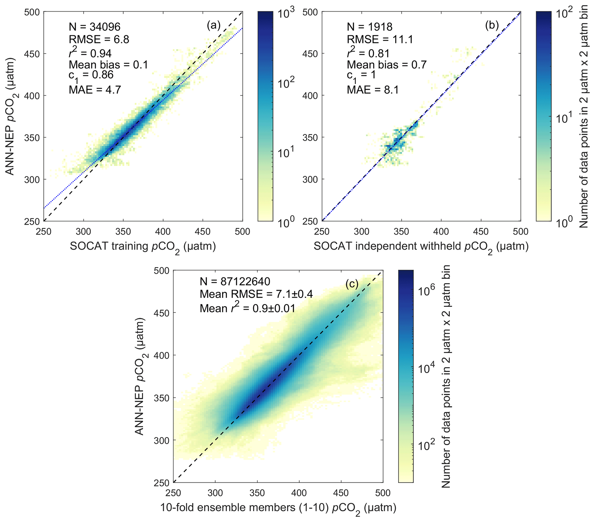
Figure 2Regional high-resolution artificial neural network northeast Pacific (ANN-NEP) ensemble mean pCO2 against (a) training pCO2 observation data and (b) independent withheld pCO2 observation data. Number of observations (N), root mean squared error (RMSE), coefficient of determination (r2), mean absolute error (MAE), mean bias (calculated as the mean residual), and the slope of the linear regression (c1). The observed linear relationship is represented by the dotted blue line. (c) ANN-NEP pCO2 (ensemble mean) against individual ensemble member estimates. Total number of observations (N) across all 10-fold ensemble members (see Sect. 2.5). Across all panels, data are binned into 2 µatm by 2 µatm bins. The dashed black line represents a perfect fit of slope (c1) = 1 and intercept = 0. Color bar shows data density on a log scale. Note the order-of-magnitude difference in the color bar scale between panels.
The ANN ensemble model mean approach demonstrated improved performance metrics when compared to each individual ensemble member. The ensemble median was nearly equivalent to the ensemble mean (r2=0.99; not shown). Overall, individual ensemble members showed little deviation (RMSE < 8 µatm) from the ensemble mean (Fig. 2c), with the ensemble mean still improving estimate robustness and reducing overtraining as evident in comparing the final ANN product to independent withheld data (Fig. 2b) and the mean RMSE of individual ensemble members to independent withheld data (13 ± 1 µatm; Fig. S4a). Each individual ensemble member also performed relatively well compared to the 10 % subsample of corresponding 10-fold evaluation data (mean RMSE = 17 ± 2 µatm; Fig. S4b). The mean standard deviation across all grid cells within the 10-fold ensemble is 2.2 ± 1.3 µatm (mapped in Fig. S5).
3.2 Uncertainty calculations
Uncertainty in the ANN-estimated pCO2 product was calculated following Landschützer et al. (2018, 2014), Roobaert et al. (2019), and Keppler et al. (2020) (Eq. 2), where the overall pCO2 product uncertainty () is calculated from the square root of the sum of the four squared errors: observational uncertainty (θobs), gridding uncertainty (θgrid), ANN interpolation uncertainty (θmap), and ANN run randomness uncertainty (θrun).
Observational uncertainty (θobs=3.1 µatm) is the measurement uncertainty in pCO2 in the field, evaluated as the average of the uncertainty assigned to each data point according to its SOCAT quality control (QC) flag (between 2–5 µatm). Gridding uncertainty (θgrid=1.5 µatm) is associated with gridding SOCAT observations into monthly ∘ × ∘ bins, evaluated as the average standard deviation among pCO2 values within each grid cell with at least three data points. ANN interpolation uncertainty (θmap=11.1 µatm) is uncertainty introduced by interpolating the pCO2 observations using the SOM-FFN approach, evaluated as the RMSE from the ANN ensemble output compared to the independent withheld SOCAT data (Fig. 2b). One limitation of our approach in assessing the uncertainty in the ANN interpolation method is that it is only applicable to grid cells where observations are available. Consequently, location-specific seasonal biases, especially at high latitudes with limited wintertime observations (Fig. 1a, b), may not be fully captured or accounted for. The standard deviation of the ensemble (ensemble spread) gives an indication of how robust our estimate is from one run to the next using different 10-fold training data (Sect. 2.5; Keppler et al., 2020). ANN run randomness uncertainty (θrun=2.2 µatm) comes from the mean standard deviation between 10-fold ensemble members (Sects. 2.5 and 3.1), which is less than the comparison of each member of the ensemble with the ensemble mean (Figs. S4; 2c).
Overall product uncertainty combining all four components according to Eq. (2) is 12 µatm, with the contribution of ANN interpolation uncertainty being the largest. Our product uncertainty is comparable to reported open-ocean uncertainty values from global products (Landschützer et al., 2014) as well as a regional product in the California Current System (Sharp et al., 2022). Combining the reported uncertainty in the gas transfer velocity (Sect. 2.6) and the overall pCO2 product uncertainty yields an average uncertainty of ±0.24 mol m−2 yr−1 in the air–sea gas flux, with the largest fraction of the error stemming from the uncertainty in the gas transfer velocity. The total uncertainty in the flux corresponds to roughly 20 % of individual grid cell calculated flux values.
3.3 Improvement relative to a global product
The ANN-NEP pCO2 product created here shows improved performance over the Landschützer et al. (2020b) global product at each time step within the study area when compared to SOCAT data gridded at ∘ × ∘ (Fig. 3), illustrating the importance of regional high-resolution estimates in resolving fine-scale variations. Across all evaluation metrics the global product does not perform as well in the region compared to SOCAT training data (RMSE = 14; r2=0.74; mean bias = −2; c0=0.68; MAE = 10; compared to Fig. 2a). This improvement suggests that a regional high-resolution product can narrow the range of variability in predictor data within the SOM clustering step and present pCO2 observation data with a greater correlation to the FFN. In the Landschützer et al. (2020b) global product, there is often only one SOM biogeochemical province covering the whole region, forcing nonlinear relationships in the FFN to be built around greater variability in pCO2 observation data from a wider range of geographic areas. The ANN-NEP regionally specific four SOM biogeochemical province grouping could alleviate this shortcoming in the FFN step. The improvement in our high-resolution product is particularly evident in the seasonal amplitude, where differences between ANN-NEP and Landschützer et al. (2020b) exceed the product uncertainty in 25 % of grid cells (Fig. S6a). The largest seasonal amplitude differences occur in the north Alaskan Gyre region and south of the North Pacific Current (Fig. S6a). The additional spatial resolution and temporal details in the regional high-resolution product provide key information to inform future observation programs including potential mooring locations. The value added in stepping to a high-resolution regional product proves particularly useful in resolving biogeochemical gradients within the subpolar Alaskan Gyre system in our study area (Sect. 4).
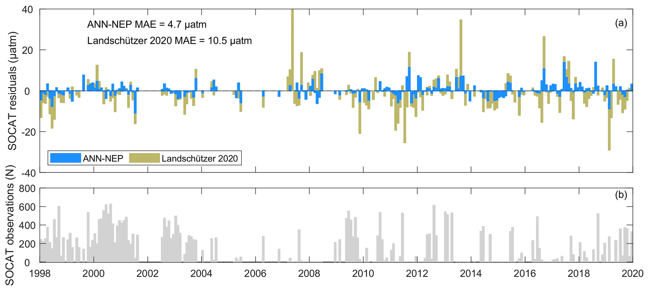
Figure 3(a) Mean residuals over the full study area at each time step of the ANN-NEP pCO2 estimate in this study and the Landschützer et al. (2020b) product interpolated to the ∘ × ∘ grid of this study, compared to the gridded SOCAT data displaying the mean absolute error (MAE). (b) Total number of gridded SOCAT observations across the study area at each time step.
3.4 Performance at coarser resolutions
Stepping to a higher spatial resolution drastically decreases the ratio of gridded pCO2 observations compared to the total number of grid cells (Fig. 4f); nevertheless, the ANN experiences minimal loss in performance across different spatial resolutions (Fig. 4a–e). Globally, most open-ocean observation-based pCO2 products are interpolated onto a 1∘ × 1∘ gridded resolution (Landschützer et al., 2020b; Global Ocean Surface Carbon, EU Copernicus Marine Service Information MULTIOBS_GLO_BIO_CARBON_SURFACE_REP_015_008, 2022; Denvil-Sommer et al., 2019; Zhong et al., 2022), with most coastal or regional products using a ∘ × ∘ grid cell size (Laruelle et al., 2017; Sharp et al., 2022; Hales et al., 2012; Nakaoka et al., 2013), with a few regional products stepping to even higher resolutions (e.g., 1 km in Chen et al., 2016; 4 km in Parard et al., 2015, 2016; 11 km in Xu et al., 2019). To determine how the network performs when producing a coarser-resolution product, we tested the same configuration of our tuned ∘ × ∘ ANN at various resolutions (Fig. 4). The predictor variables and SOCAT pCO2 observations were simply bin-averaged to coarser grid cell sizes (i.e., 1, , , ∘).
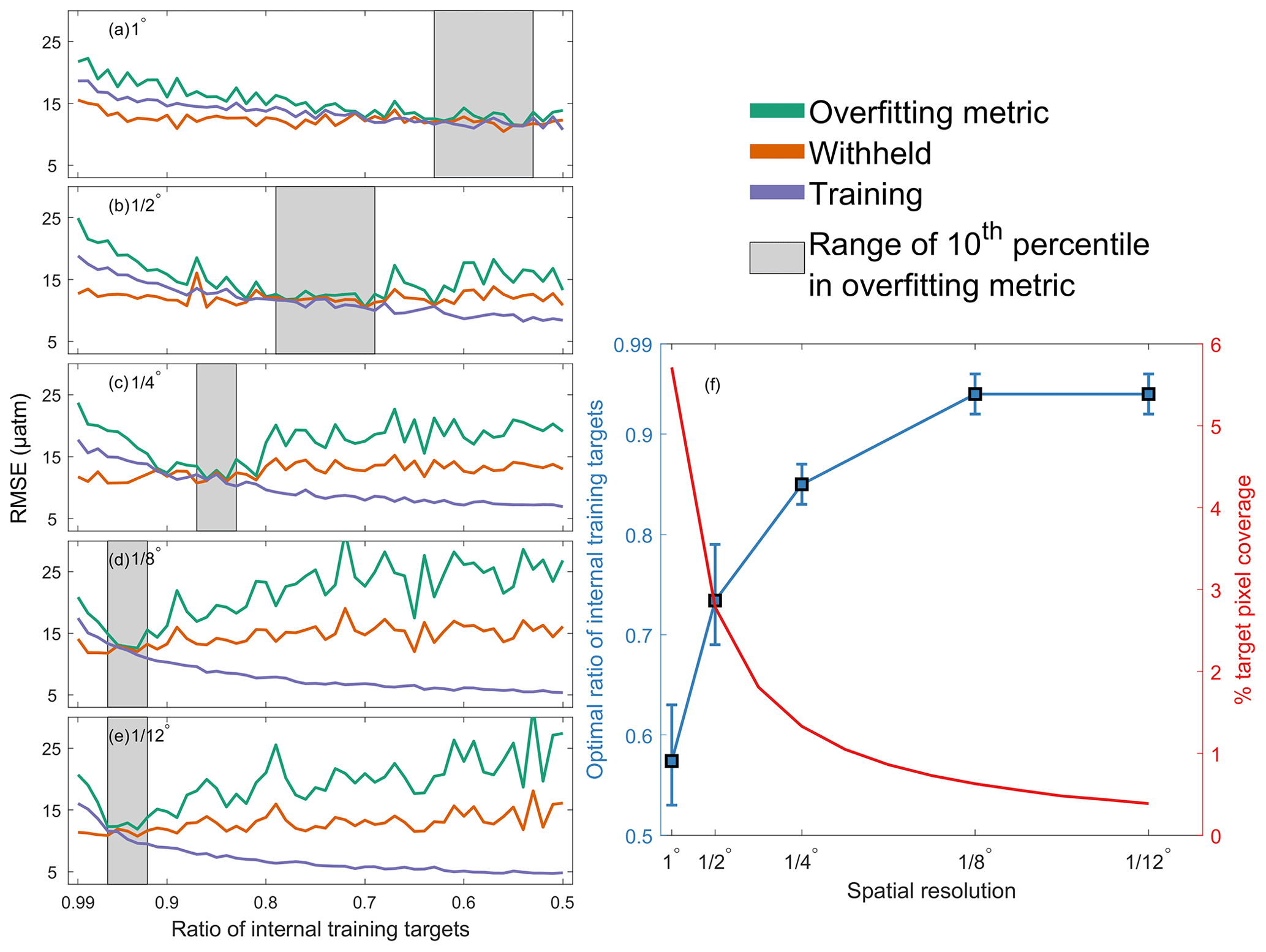
Figure 4Varying spatial resolution: (a) 1∘, (b) ∘, (c) ∘, (d) ∘, and (e) ∘ ANN pCO2 product performance evaluated by the mean RMSE (Sect. 2.3) of training data (blue line), independent withheld data (orange line), and an overfitting metric (green line; Sect. 3.4) against internal data division ratios of the pCO2 training data used by the ANN to train and internally evaluate. The ratios in gray show the range of the lower 10th percentile (5 of 50 runs) of overfitting metric values for each resolution. (f) At each spatial resolution, the left-hand y axis shows the optimal internal data division ratio with error bars representing the lower 10th percentile of overfitting metric values (same as gray ranges in a to e with all resolutions converging around RMSE = 12.8 ± 0.4 µatm). The right-hand y axis shows the percent of gridded pCO2 observations (targets) compared to the total number of grid cells.
Using the same ANN configuration between the different resolutions (i.e., optimal SOM biogeochemical provinces, appropriate predictors, neuron number in the first hidden layer, etc.; see Sect. 2.5), the most important parameter for reducing overfitting at each resolution becomes the internal data division ratio between the pCO2 training data used by the ANN to train and internally evaluate (Fig. 4). We tested a suite of data division ratios between 99 % of data used to train and 1 % used to internally evaluate to a split at 1 % intervals for each resolution (Fig. 4). These tests were run without the 10-fold cross-evaluation ensemble approach. To quantify the optimal ratio at each resolution, we used an overfitting metric (Eq. 3) equal to the larger of the training or independent withheld data RMSE plus the absolute value of the difference between the two:
Using an internal data division ratio optimized based on the overfitting metric, an ANN interpolated pCO2 product with an uncertainty value of 12.5 ± 0.4 µatm (see Sect. 3.2; Table S2) is possible at each of the coarser resolutions (Fig. 4a–e; Table S2). For comparison, the reported uncertainty in a global product (Landschützer et al., 2014) ranges from 9 to 18 µatm. In regions with sufficient observational coverage (Fig. 4f; Bakker et al., 2016), this finding creates a precedent for stepping to a higher-resolution product with nearly no loss in performance, overcoming the overfitting concern with increased resolution (Rosenthal, 2016).
With the estimated ANN pCO2 product displaying a strong ability to accurately represent regional pCO2 variability in the northeast Pacific (Sect. 3), we calculate air–sea CO2 fluxes in the region (Eq. 1). Long-term (1998–2019) mean pCO2 and air–sea CO2 fluxes display similar patterns (Fig. 5). In the northwest of our study area, high pCO2 and net CO2 outgassing to the atmosphere correspond to the influence of the upwelling subpolar Alaskan Gyre system (Figs. 5; 1c). Lower pCO2 values and stronger atmospheric CO2 uptake occur in the North Pacific Current region (Fig. 1c) to the south and along the eastern study area margin (Fig. 5). The gradient of the gyre captured in the high-resolution estimate improves regional understanding, with the largest differences between the Landschützer et al. (2020b) global product occurring in the north (basin-wide absolute difference 2 %–5 %; Fig. S6a). ANN-NEP calculated fluxes compare well to air–sea CO2 fluxes averaged across six unique, coarser-resolution, global-observation-based pCO2 products, each using five different wind speed products (r2=0.81; Fay et al., 2021). However, our work suggests that the global product ensemble may underestimate the outgassing signal from the subpolar Alaskan Gyre (Figs. 5b; S7). A higher resolution in the gyre gradient also provides regional context to carbon measurements made at the Ocean Station Papa mooring, often used to represent the Alaskan Gyre (e.g., Jackson et al., 2009), which is actually situated approximately between the two regions and along the Line P monitoring program.
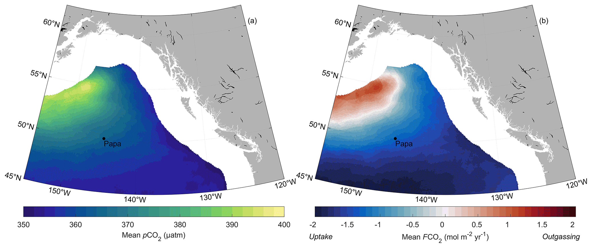
Figure 5(a) Long-term (1998–2019) mean ANN-NEP pCO2 and (b) air–sea CO2 flux density in mol m−2 yr−1 for the open-ocean northeast Pacific. Negative (positive) flux values indicate CO2 uptake (outgassing) by the ocean. Ocean Station Papa is shown for reference.
4.1 Seasonal variability
To determine seasonal cycle drivers, we decompose the climatological pCO2 into a thermal and non-thermal component (Takahashi et al., 2002, 1993):
Here the subscripts T and NT represent thermal and non-thermal effects, respectively, while subscripts am and mm represent annual mean and monthly mean values, respectively. Equation (4) imposes the empirical temperature dependency on the annual mean pCO2 value, providing an estimate of seasonal temperature control (Sarmiento and Gruber, 2006; Takahashi et al., 2002). Equation (5) removes the temperature dependency from the monthly mean pCO2 values, providing an estimate of the residual, non-thermal controls on pCO2 including circulation, mixing, gas exchange, and biology. The ratio of the seasonal amplitudes of the two components (Eq. 6; ) can distinguish the dominant process, where a value greater (less) than 1 indicates that thermal (non-thermal) processes dominate.
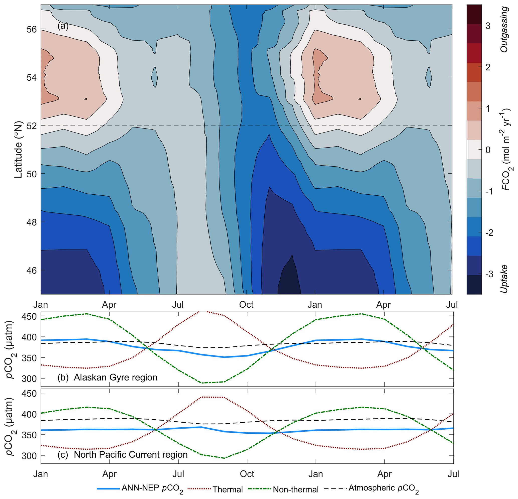
Figure 6(a) Zonally averaged air–sea CO2 flux from the ANN-estimated pCO2 product climatology along each ∘ latitude band in the study area plotted against the climatological month along the x axis (Hovmöller diagram). Negative (positive) flux values indicate CO2 uptake (outgassing) by the ocean. The dashed gray line subdivides the Alaskan Gyre and North Pacific Current regions in the north and south with different seasonal drivers summarized in panels below. (b) Alaskan Gyre region (latitudes north of 52∘ N) and (c) North Pacific Current region (latitudes south of 52∘ N) area-averaged monthly climatological pCO2 (solid blue line), thermal component (i.e., changes due to temperature; Eq. 4; dotted red line), non-thermal component (i.e., changes due to circulation, mixing, gas exchange, and biology; Eq. 5; dot–dash green line), and atmospheric pCO2 (dashed black line). The climatology is plotted over 19 months to emphasize the seasonal cycle.
Seasonally, the northern Alaskan Gyre region of our study area (latitudes north of 52∘ N; Fig. 6a, b) flips from outgassing in the wintertime to uptake in the summer in the climatological air–sea CO2 flux (Brady et al., 2019; Palevsky et al., 2013; Chierici et al., 2006). The change in the sign of the flux is driven by a 40 µatm difference between winter maximum and summer minimum pCO2 climatology values (Fig. 6b). In the Landschützer et al. (2020a) climatology, this seasonal dipole in the Alaskan Gyre also exists, displaying a 40 µatm seasonal pCO2 range. Similar patterns exist in the Takahashi et al. (2014, 2009, 2002) climatologies as well (approximately 45–50 µatm). Increased wind stress curl drives stronger gyre circulation in the fall and winter, upwelling and entraining nutrient- and CO2-rich subsurface waters into the surface ocean, increasing the non-thermal pCO2 component (Fig. 6b) and leading to outgassing (Fig. 6a; Chierici et al., 2006). Through the spring and summer, biological drawdown, preconditioned by the upwelled, mixed, and entrained nutrients, decreases the surface ocean non-thermal pCO2 component (Fig. 6b; Harrison et al., 1999), enhancing uptake (Fig. 6a). Although the seasonal amplitude of the temperature component is also large in the north, these non-thermal controls dominate ().
In the south part of our study area, the North Pacific Current region (latitudes south of 52∘ N; Fig. 6a, c) acts as a strong CO2 sink through the winter, transitioning to a weak sink through the summer. Whereas in the Alaskan Gyre region the seasonal cycle of pCO2 is dominantly controlled by non-thermal drivers (Fig. 6b), the North Pacific Current region experiences a near-balance between opposing drivers (Fig. 6c; ). In the North Pacific Current region, we see a much smaller seasonal amplitude in pCO2 (15 µatm; Fig. 6c), peaking in July with warming and falling to a minimum in October. The seasonal amplitude is dampened by the competing effect of temperature changes in solubility and changes in dissolved inorganic carbon concentration through biological drawdown and changing mixed layer depth (Wong et al., 2010; Sutton et al., 2017). With minimal seasonal variation in seawater pCO2, the seasonal change in atmospheric CO2 uptake south of 52∘ N (Fig. 6a) is dominantly driven by higher wind speed through the winter months (mean increase of 55 % over summer climatological values).
4.2 Alaskan Gyre upwelling strength
On sub-decadal to decadal timescales, there is a strong correlation between air–sea CO2 flux anomalies and SSH anomalies in the Alaskan Gyre region of our study area (r2=0.93, p<0.01; Figs. 7b, c; S8). In this subpolar gyre, prevailing winds cause upwelling driven by Ekman pumping (Gargett, 1991), but the strength varies. During 1998–2002 as well as 2006–2013, we observe strong winter and spring outgassing in the Alaskan Gyre, with flux densities as high as 3.6 mol m−2 yr−1 in January 2000. In these same periods, anomalously low sea level pressure over the Alaskan Gyre led to anomalously strong wind stress curl which enhanced Ekman pumping and depressed SSH (Fig. 7b; Mann and Lazier, 2006; Hristova et al., 2019). The stronger upwelling brought CO2-rich subsurface water to the surface (Lagerloef et al., 1998). Conversely, during the periods of anomalously high sea level pressures and positive SSH anomalies (2003–2005; 2014–2020; Fig. 7c), there is less upwelling of CO2-rich subsurface water to the surface, allowing primary productivity to draw down surface ocean CO2 (McKinley et al., 2006) and enhancing CO2 uptake from the atmosphere (Fig. 7b).
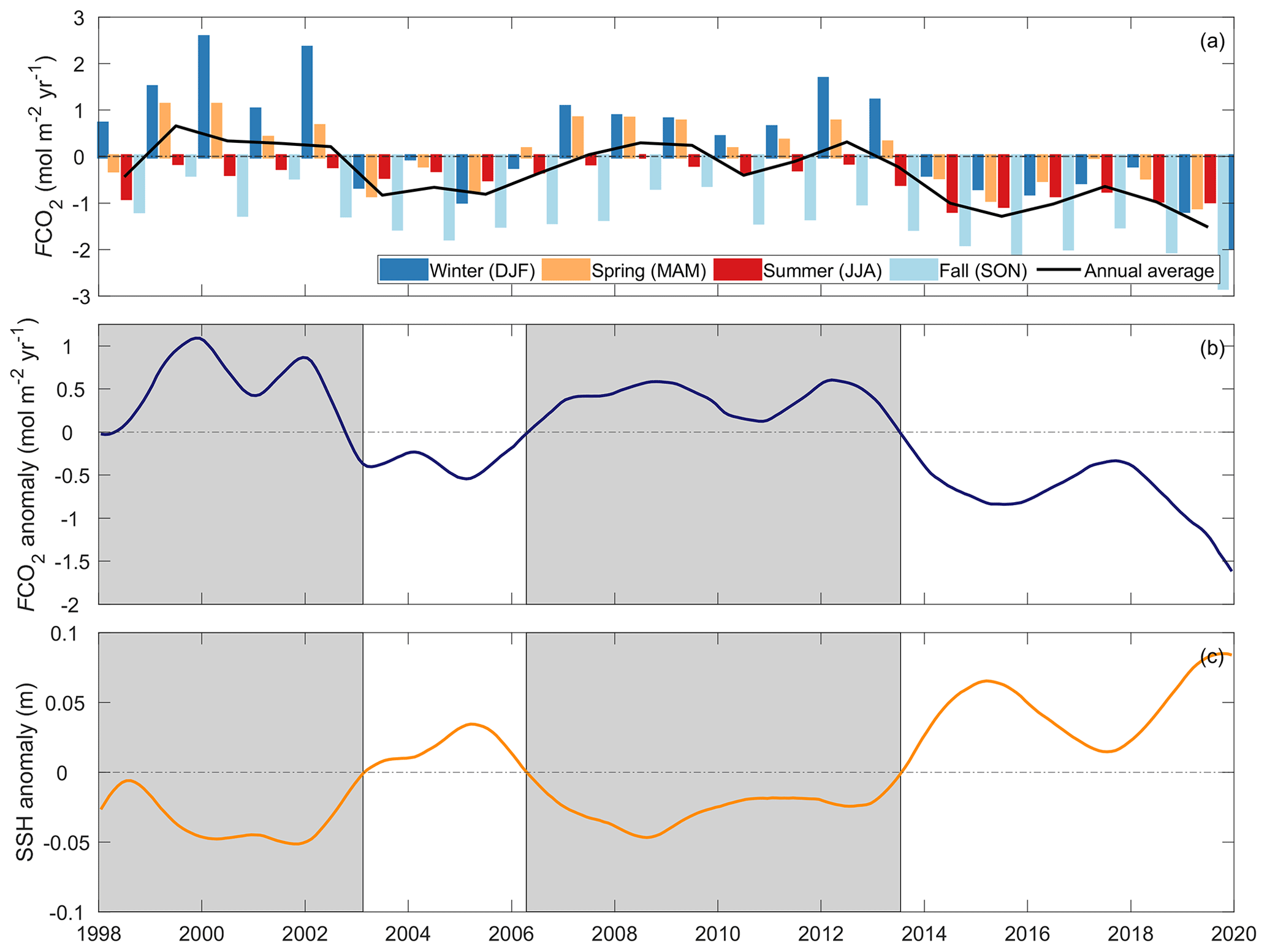
Figure 7Alaskan Gyre region of our study area (latitudes north of 52∘ N). (a) Air–sea CO2 fluxes grouped by seasonal 3-month bins along with the annual average (black line). (b) Air–sea CO2 flux anomalies removing the seasonal cycle (Sect. 2.4) and applying a 12-month running mean. (c) Sea surface height (SSH) anomalies in the same region removing the seasonal cycle and applying a 12-month running mean. Gray boxes highlight periods of anomalously high Alaskan Gyre upwelling strength corresponding to negative SSH anomalies. Horizontal dashed lines mark 0 in each panel. Seasonal groupings in (a) are winter (December, January, February), spring (March, April, May), summer (June, July, August), and fall (September, October, November).
Our observation-based findings show strong carbon relationships with SSH in the Alaskan Gyre, with correlations between other climate indices being weaker. Over longer timescales, climate-driven regional ocean fluctuations have been shown to modulate the Alaskan Gyre surface water inorganic carbon system (Hauri et al., 2021; Di Lorenzo et al., 2008). The North Pacific Gyre Oscillation and the Pacific Decadal Oscillation indices have both been shown to strongly influence the physics, chemistry, and biology of the Gulf of Alaska ecosystem (Di Lorenzo et al., 2008; Newman et al., 2016). Hauri et al. (2021) showed that the rate of ocean acidification in a hindcast model of the Gulf of Alaska was strongly related to the first empirical orthogonal function of SSH. We report the same relationship with SSH described in Hauri et al. (2021) as the dominant control of sub-decadal patterns on air–sea CO2 fluxes from our observation-based pCO2 product (Fig. 7). Our estimates of the 12-month running mean air–sea CO2 flux anomaly in the Alaskan Gyre region (Fig. 7b) are more weakly correlated to the North Pacific Gyre Oscillation, Pacific Decadal Oscillation, and the El Niño–Southern Oscillation indices (r2=0.63, 0.38, 0.22 respectively; p<0.01). This regional variation in SSH correlating with both observations and models is strong evidence for variations in Alaskan Gyre upwelling strength explaining regional biogeochemistry on sub-decadal to decadal timescales. This relationship supports work showing that the SSH anomaly is an important climate index for the region (Cummins et al., 2005; Di Lorenzo et al., 2008). This finding also highlights the challenges of representing the regional seasonal cycle of the northeast Pacific in a climatology within a reference period dominated by one mode of Alaskan Gyre upwelling strength.
4.3 Impact of interannual events
On shorter, interannual timescales, basin-wide variability in air–sea CO2 flux is significantly influenced by the impact of extreme events, with the underlying sub-decadal and decadal signal amplifying or dampening these impacts. During persistent marine heat waves in the northeast Pacific since 2013, we see strong atmospheric CO2 uptake anomalies fueled by reduced winter mixing and increased surface density stratification (Fig. 8; Bond et al., 2015). The strongest marine heat wave, known as “the Blob”, with sea surface temperature anomalies greater than 3 ∘C or 4 standard deviations above normal (Freeland and Ross, 2019), persisted in the northeast Pacific from late 2013 to the end of 2015 driven by an anomalous high-pressure atmospheric ridge (Bond et al., 2015; Di Lorenzo and Mantua, 2016). The ridge was associated with a significant decline in local wind speed, decreasing the mixing of deep, colder waters to the surface and raising sea surface temperatures (Bond et al., 2015; Scannell et al., 2020). The reduced winter mixed layer deepening and associated limiting of upwelled and entrained nutrient and CO2-rich subsurface waters to the surface have been linked to a relief of ocean acidification (i.e., anomalously high aragonite saturation states; Mogen et al., 2022). There has also been a reported increase in net primary production during the Blob in both in situ and satellite records (Long et al., 2021; Yu et al., 2019; Peña et al., 2019). During the Blob, we see strong negative air–sea CO2 flux anomalies, particularly in the winter months (October to December 2014 and 2015), indicative of a 30 % increase in uptake relative to climatological monthly means. The increased atmospheric CO2 uptake is driven by reduced winter wind speeds (by approximately 7 %), leading to limited winter mixed layer deepening and increased surface density stratification, while possibly being enhanced by the increase in net primary production (Fig. 8b).
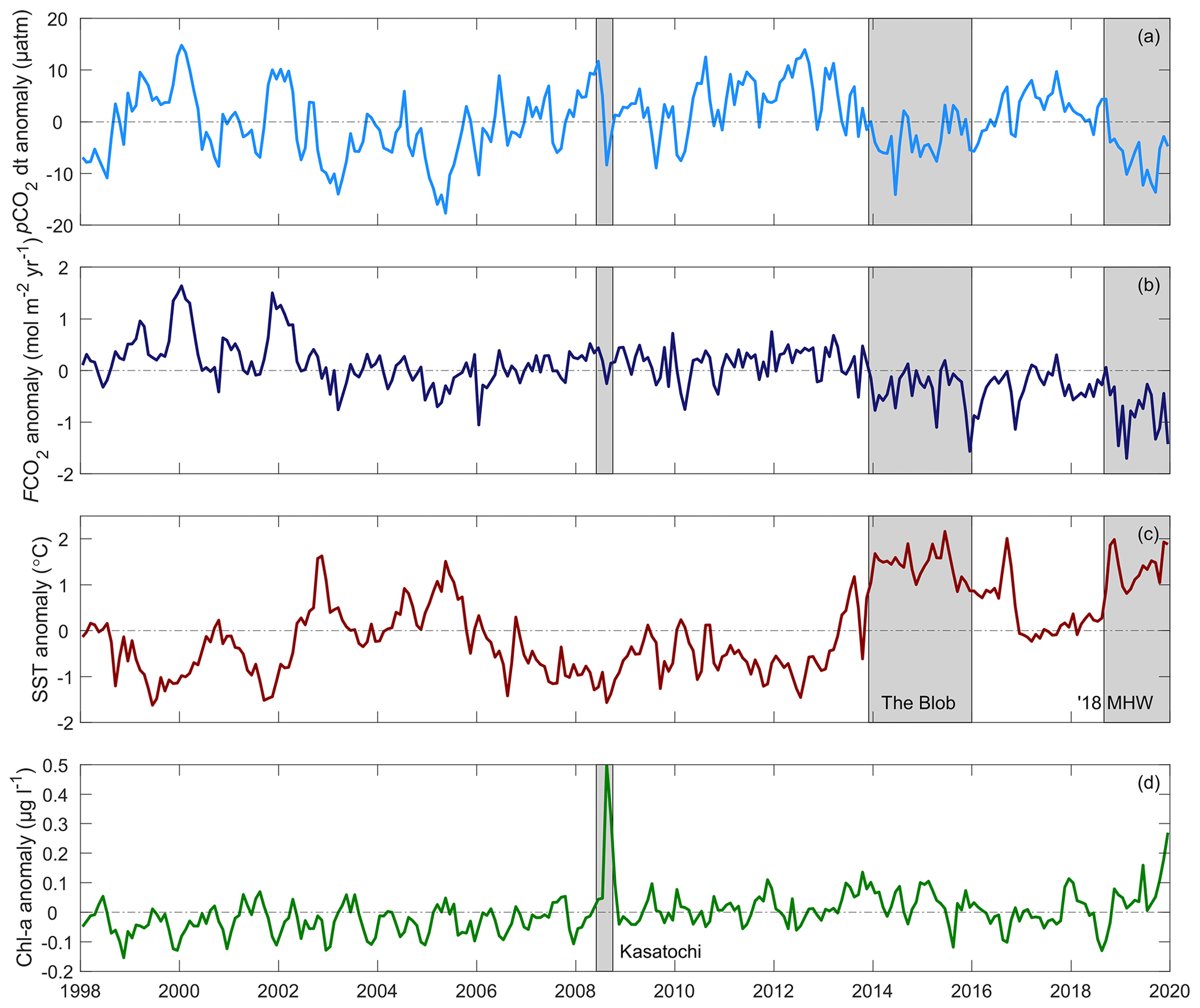
Figure 8Full study-area-averaged interannual variability in (a) pCO2 anomaly removing the seasonal cycle (Sect. 2.4) and long-term trend (Sect. 4.4). In addition, (b) air–sea CO2 flux anomaly, (c) sea surface temperature anomaly, and (d) chlorophyll-a anomaly all removing the seasonal cycle. Gray boxes highlight large interannual events including the Blob marine heat wave in 2014–2016, a second marine heat wave in 2018–2020 (labeled “'18 MHW” in the figure), and a 2008 ocean iron fertilization event following the Kasatochi volcanic eruption (Kasatochi). Horizontal dashed lines mark 0 in each panel.
Through a second marine heat wave from mid-2018 to 2020 (Chen et al., 2021; Amaya et al., 2020; Scannell et al., 2020), we see a similar magnitude increase in atmospheric CO2 uptake compared to the Blob event (Fig. 8b). Through some of the largest SST anomalies (October to December 2018 and 2019), we observed large negative air–sea CO2 flux anomalies indicating enhanced atmospheric uptake of 45 % beyond corresponding climatological monthly means (Fig. 8b), particularly in the Alaskan Gyre (Fig. 7a, b). During this marine heat wave, a similar reduction in upper-ocean mixing and limited wintertime entrainment due to reduced wind speed were observed (by approximately 9 %; Amaya et al., 2020) along with resultant reduced surface pCO2 (Franco et al., 2021). Increased net primary production has also been reported (Long et al., 2021). An unusual near-surface freshwater anomaly in the Gulf of Alaska during 2019 contributed to the intensification of the marine heat wave by increasing the near-surface buoyancy and density stratification (Scannell et al., 2020).
Our result that marine heat waves cause enhanced CO2 uptake in the northeast Pacific may not be applicable to a wider region. Mignot et al. (2022) described how the impact of marine heat waves on air–sea CO2 fluxes is the net result of two competing mechanisms: (1) increased sea surface temperatures reducing the solubility of CO2, increasing pCO2, and reducing CO2 uptake and (2) increased density stratification reducing vertical mixing and entrainment, decreasing surface dissolved inorganic carbon, and increasing CO2 uptake. Their analysis finds that the temperature effect outweighs the advection effect during persistent marine heat waves in the North Pacific subtropical gyre, reducing CO2 uptake by 29 ± 11 %, with the opposite true in the tropical Pacific (Mignot et al., 2022). However, when looking at our more localized study area in the northeast Pacific subpolar gyre, we find instead that the impact of reduced winter mixing (because of decreased winds and increased density stratification) tipped the balance toward enhanced atmospheric CO2 uptake during these marine heat waves, again advocating for the need for high-resolution local studies to better understand local climate change effects.
Through both the Blob and the 2019 marine heat wave, the Alaskan Gyre was in a period of weak upwelling (Fig. 7c), leading to a decade-long negative pCO2 anomaly (Fig. 8a), in addition to the maximum observed ΔpCO2 due to the diverging long-term trend from the atmosphere (Sect. 4.4). Unraveling the individual influence of these interconnected drivers (i.e., marine heat waves, sub-decadal variability, and long-term trend) is not possible with this product but does prompt future inquiry in combination with regional models and emerging climate analysis tools (e.g., Chapman et al., 2022).
We do not observe a large change in atmospheric CO2 uptake associated with the 2008 basin-wide ocean iron fertilization event. In August 2008, the eruption of the Kasatochi volcano in the Aleutian Islands, Alaska, USA, dispersed volcanic ash over an unusually large area of the subarctic northeast Pacific, fueling a massive phytoplankton bloom in the iron-limited region (Langmann et al., 2010; Hamme et al., 2010). Hamme et al. (2010) reported that enhanced biological uptake drew down pCO2 by approximately 25 µatm at Ocean Station Papa. Basin-wide, we see a decrease of 20 µatm from July to August 2008 in the detrended, de-seasonalized ANN pCO2 following the eruption (Fig. 8a) with a drawdown of 30 µatm at Ocean Station Papa. The neural network approach does display a tendency to slightly overestimate relatively low pCO2 values (Fig. 2a). Because this basin-wide enhanced primary production and surface ocean pCO2 decrease lasted only 2 months, its impact on the air–sea CO2 flux was limited (Fig. 8b). The limited impact could be tied to weaker summer wind speeds and longer equilibration times (Jones et al., 2014). The eruption occurred during a period of enhanced Alaskan Gyre upwelling (Fig. 7c), meaning the event was overlaid on top of an already sub-decadal-length positive pCO2 anomaly (Fig. 8a) perhaps dampening the event's impact. Unfortunately, the lack of direct pCO2 measurements in SOCAT v2021 during this time prevents us from further investigating the underlying causes.
4.4 Air–sea CO2 flux trend
Overall, the northeast Pacific Ocean CO2 sink became more negative (i.e., become a larger sink; Fig. 9b) from 1998 to 2020 at a rate of mol m−2 yr−2. Looking at the start and end of the time series, the average flux from 1998 to 2002 appeared to be a small atmospheric CO2 sink at mol m−2 yr−1, compared to the sink from 2016–2020 at mol m−2 yr−1. Regionally, we do not see a statistically significant trend in the satellite-based ocean surface wind speed data over this time (p>0.1; Mears et al., 2019). However, the time series endpoints are representative of different Alaskan Gyre upwelling modes (Fig. 7c), with the time series starting in a sub-decadal-length positive pCO2 anomaly and ending during a decade-long negative pCO2 anomaly. Decadal trends will be sensitive to the start and endpoint of the time series (e.g., Fay and McKinley, 2013). We caution that our trend results may not be representative of longer time periods (i.e., from industrial onset).
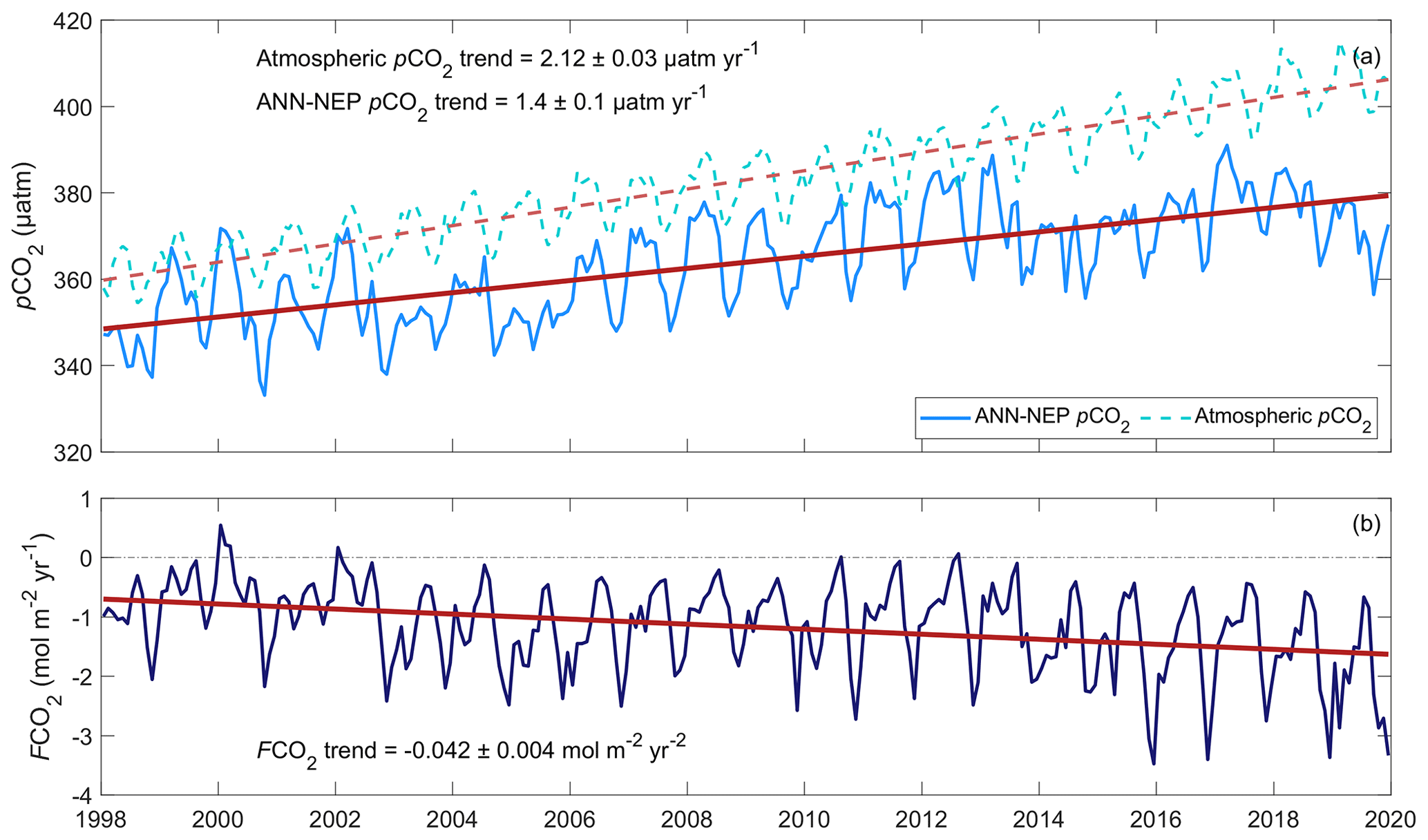
Figure 9Full study-area-averaged long-term trends in (a) ANN-NEP surface ocean pCO2 (solid line) and atmospheric pCO2 (dashed line) and (b) air–sea CO2 flux density.
Taking the full study area de-seasonalized (Sect. 2.4), averaged pCO2, we calculated trends based on shorter time series within our data using different monthly time series start and end dates (Fig. 10). Based on pCO2 data time series ranges greater than 10 years (between 1998 and 2020), 87 % of trends are less than the atmospheric trend with a mean of 1.59 ± 0.27 µatm yr−1 (N=9222 at a monthly time step; Fig. 10). In the remaining 13 % of total time series start and end date combinations, there is a pronounced very steep trend exceeding the atmospheric rate of increase. Date combinations resulting in trends exceeding the atmospheric increase could be partly attributed to start and end dates coinciding with periods of weak and strong Alaskan Gyre upwelling, respectively. These upwelling modes induce negative and positive pCO2 anomalies, which further amplify the observed trend. However, the Alaskan Gyre region makes up only about 25 % of the total study area (region north of 52∘ N; Sect. 4.2), and trends in Fig. 10 represent the ANN-NEP full spatial domain.
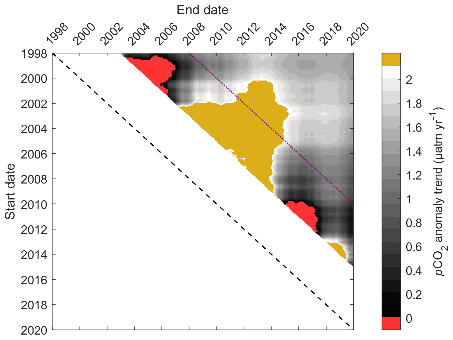
Figure 10Full study-area-averaged pCO2 anomaly (removing the seasonal cycle; Sect. 2.4) linear trend calculated using different monthly time series start and end dates. Time series start from dates on the left and end on a date along the top. The dashed black line indicates equal start and end dates. Trend values are only shown for time series of at least a 5-year duration. Red areas represent negative pCO2 trends; gold areas represent trends greater than the atmospheric rate of increase (2.12 ± 0.01 µatm yr−1). The purple dotted line indicates a 10-year time series duration.
The rate of change in the air–sea CO2 flux over the study period is largely due to the increasing gradient with the atmosphere (Fig. 9a). Over the full study area from 1998–2020, the ANN-NEP pCO2 trend is 1.4 ± 0.1 µatm yr−1. The Landschützer et al. (2020b) global product trend in the region is similar at 1.5 ± 0.1 µatm yr−1. At Ocean Station Papa, the ANN-NEP pCO2 trend is 1.5 ± 0.1 µatm yr−1, in agreement with the observed trend based on discrete samples collected one to three times per year (1.6 ± 0.8 µatm yr−1 between 1990–2019; Franco et al., 2021). The oceanpCO2 trend is not as rapid as the atmospheric increase of 2.12 ± 0.03 µatm yr−1 over the same period (Fig. 9a). Sutton et al. (2017) also reported a lag with the atmosphere at Ocean Station Papa with a ΔpCO2 trend of µatm yr−1 from the 2007–2014 mooring pCO2 data. The ANN-NEP ΔpCO2 trend at Ocean Station Papa is µatm yr−1.
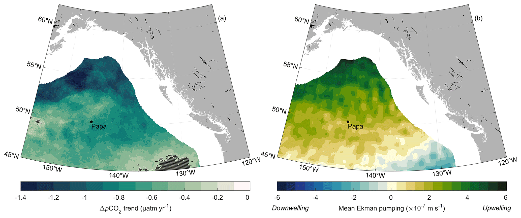
Figure 11(a) Trend in ΔpCO2 where more negative (darker) values indicate an increasing gradient with the atmosphere and a lag in the pCO2 increase in the surface ocean. Black crosshatches show grid cells with an insignificant calculated trend (outside the 95 % confidence level; p≥0.05). (b) Calculated average vertical velocity associated with Ekman pumping (calculated from zonal and meridional wind speed) where negative (blue) values indicate downwelling and positive (green) values indicate upwelling. Ocean Station Papa is shown for reference.
The observed lag in the increase in surface ocean pCO2 with respect to atmospheric pCO2, causing an increasing air–sea gradient (ΔpCO2), may be attributed to interaction with subsurface water. We find a strong spatial correlation between the trend in ΔpCO2 and the calculated average vertical velocity associated with Ekman pumping (r2=0.64, p<0.01; Fig. 11b). Ekman pumping was calculated using the MATLAB Climate Toolbox Ekman function (Greene et al., 2019, 2017; Kessler, 2002) from monthly ∘ spatial-resolution Cross-Calibrated Multiplatform zonal and meridional ocean surface wind speeds (Mears et al., 2019) interpolated to ∘. Fay and McKinley (2013) describe regions impacted by upwelling from depth having shallower pCO2 trends and greater divergence from the atmosphere based on models and observations. Dissolved inorganic carbon increases with depth, causing enhanced vertical mixing to increase surface ocean pCO2 over the seasonal cycle (Sect. 4.1 to 4.3). However, in the long term, dissolved inorganic carbon is increasing most in surface waters, due to direct uptake of atmospheric CO2, and least at depth. The supply to the surface of subsurface waters with low anthropogenic carbon causes a lag in the rate of increase in surface ocean pCO2. The anthropogenic carbon signals in the intermediate to deep waters in this region are some of the smallest in the global ocean due to circulation patterns (Sabine et al., 2004; Gruber et al., 2019; Carter et al., 2019; Clement and Gruber, 2018). Regions within our study area with a greater connection between surface and deep waters, such as the center of the Alaskan Gyre in the north (Van Scoy et al., 1991), are experiencing the largest divergence from the atmosphere. With a joint increase in projected future wind speeds (Zheng et al., 2016; Young and Ribal, 2019; Wanninkhof and Triñanes, 2017) and a growing ΔpCO2, the region is likely to become a stronger net annual sink for atmospheric CO2.
Using a high-resolution regional neural network approach, we represent pCO2 measurement variability well in the northeast Pacific Ocean. We interpolated sparse observations using nonlinear relationships developed with a neural network approach based on predictor data from satellite and reanalysis products to create a continuous monthly pCO2 estimate at a ∘ × ∘ spatial resolution. Using a cross-evaluation ensemble approach we were able to produce a robust pCO2 product that represents regional variability with an uncertainty of 12 µatm. We found that stepping to a significantly higher spatial resolution, compared to typical open-ocean observation-based pCO2 products ( or 1∘ spatial resolution), led to nearly no loss in performance despite a much lower ratio of gridded pCO2 observations compared to the total number of grid cells. The most important parameter for reducing overfitting across regional pCO2 products with different spatial resolutions was the internal division of training data. Higher-resolution products require more direct training data and fewer data to internally evaluate, while still comparing them to independent withheld data. This work shows that high-resolution, high-performance, observation-based neural-network-derived pCO2 products can be developed when reducing the complexity of controlling processes by focusing on specific regions. However, chosen predictor variables need to be regionally specific considering “process-focused” influences on the local carbon system. Our reported optimization of the internal data division ratio between network training and evaluation data indicates the importance of this choice when moving to a higher spatial resolution. Increased spatial resolution will be necessary to capture variability in regions strongly influenced by mesoscale processes, enabling the resolution of oceanographic features such as eddies, upwelling regimes, and gyre system gradients.
We report pronounced variability in marine CO2 uptake in the northeast Pacific Ocean dominantly driven by the control of Alaskan Gyre upwelling and connectivity to subsurface waters. Overall, the open-ocean northeast Pacific acted as a net sink for atmospheric CO2 from 1998 to 2020 with an average basin-wide air–sea CO2 flux of mol m−2 yr−1 but with pronounced seasonality. In the northern Alaskan Gyre region, wintertime upwelling and entrainment lead to significant outgassing. In the southern North Pacific Current region, the seasonal flux cycle is largely driven by wind speed where the seasonal change in surface ocean pCO2 remains small. Based on our product, the upwelling strength of the Alaskan Gyre dominates air–sea CO2 flux variability in that region on sub-decadal to decadal timescales. During prolonged periods of enhanced gyre upwelling, we see strong winter outgassing driven by upwelled and entrained CO2-rich subsurface waters. During periods of weak gyre upwelling, the northern part of our study area acts as a sink for atmospheric CO2 year-round. During two recent marine heat waves we see enhanced CO2 uptake due to limited wintertime entrainment of subsurface waters resulting from weaker winds. However, we observed minimal impact on atmospheric CO2 uptake following a 2008 volcanic eruption, with air–sea CO2 flux anomalies linked to enhanced biological uptake via iron fertilization lasting only 2 months. The gradient between the northeast Pacific surface ocean pCO2 and atmospheric CO2 is increasing, pushing the region towards becoming an enhanced sink for atmospheric CO2. We see the largest increase in the gradient (and thus potential for greater future uptake) at the center of the Alaskan Gyre where, through upwelling, there is a strong connection with subsurface waters low in anthropogenic CO2.
The regional, high-resolution pCO2 product created here could serve as a valuable baseline for regional models (e.g., Pilcher et al., 2018; Hauri et al., 2020). The pCO2 product and associated air–sea CO2 flux estimates offer continuous coverage in sparsely sampled regions informed by patterns in well-sampled neighboring waters. The product could be used to aid in model evaluation, for data assimilation, to constrain initial conditions, to enhance carbon flux process understanding, and to improve regional climate change projections.
Our analysis illustrates the complex interplay between factors driving air–sea CO2 flux variability at varying temporal scales across the study domain and within broad subregions (Alaskan Gyre and North Pacific Current regions) allowing us to suggest what resources will be needed to make further advances. Improvement in estimated pCO2 would benefit from an increase in the number of pCO2 observations used for training. We recommend prioritizing additional measurements in the northern Alaskan Gyre region in future observational programs. Our estimated fluxes in the gyre are large (both uptake and outgassing), but observations are sparse, leading to the largest standard deviations between our cross-evaluation ensemble members (Fig. S4). The impact of sub-decadal to decadal variability on the trend in surface ocean pCO2 and in regional atmospheric CO2 uptake emphasizes the importance of long-duration time series sites and programs to capture the natural cycles of variability and accurately estimate change. Our findings and estimated pCO2 product serve as environmental baselines, which could be used to inform future marine carbon dioxide removal in the northeast Pacific at the basin and regional scale. However, use of our product at the individual grid cell level is not encouraged as errors likely remain high, whereas over broader regions these errors average away. Our study serves as an important initial step in creating a complete carbon budget for the northeast Pacific, with coastal, pelagic, and benthic carbon stocks and fluxes still to be resolved.
All data used are publicly available. ANN-NEP pCO2 and air–sea CO2 flux fields are available through the National Center for Environmental Information (NCEI Accession 0277836; https://doi.org/10.25921/c1w8-6v02, Duke et al., 2023a). pCO2 data are from the Surface Ocean CO2 Atlas (SOCAT) v2021 (available at https://www.socat.info/, Bakker et al., 2016), and additional data are from the Fisheries and Oceans Canada February 2019 Line P cruise (available at https://www.waterproperties.ca/linep/, Water Properties Group, 2022). Sea surface temperature and chlorophyll a are from the European Space Agency Climate Change Initiative (available at https://climate.esa.int/en/odp/#/dashboard, European Space Agency, 2019). Sea surface salinity, sea surface height, and mixed layer depth are from the Copernicus Marine Environment Monitoring Service (available at https://data.marine.copernicus.eu/product/GLOBAL_MULTIYEAR_PHY_001_030/description, E.U. Copernicus Marine Service, 2022). Ocean surface wind data are from the Cross-Calibrated Multiplatform version 2 Wind Vector Analysis Product (available at https://www.remss.com/measurements/ccmp/, Mears et al., 2019).
The supplement related to this article is available online at: https://doi.org/10.5194/bg-20-3919-2023-supplement.
PJD and PL developed the neural network code and created the product with help from RCH, DI, NCS, and MMMA. PJD, RCH, DI, and PL contributed to the interpretation and analysis of the results. All co-authors contributed to editing the paper. RCH and DI supervised the project work. PAC provided data and consultation. PJD prepared the paper with contributions from all co-authors.
At least one of the (co-)authors is a member of the editorial board of Biogeosciences. The peer-review process was guided by an independent editor, and the authors also have no other competing interests to declare.
This article reflects only the authors' view – the funding agencies as well
as their executive agencies are not responsible for any use that may be made
of the information that the article contains.
Publisher's note: Copernicus Publications remains neutral with regard to jurisdictional claims in published maps and institutional affiliations.
Ocean Station Papa mooring time series site and the Line P Program are operated by the National Oceanic and Atmospheric Administration (NOAA) and Fisheries and Oceans Canada (DFO). Thanks to Marine Fourrier and one anonymous reviewer for their helpful comments improving the paper.
Funding for this project to Roberta C. Hamme was provided by the Natural Sciences and Engineering Research Council of Canada (NSERC) through the Advancing Climate Change Science in Canada program (grant no. ACCPJ 536173-18). Funding from Fisheries and Oceans Canada's Aquatic Climate Change Adaptation Service Program to Paul Covert supported the analysis of recent underway pCO2 measurements made by the Line P Program (grant no. 96036). Patrick J. Duke's financial support was also provided by a Natural Sciences and Engineering Research Council of Canada (NSERC) Doctoral Postgraduate Scholarship.
This paper was edited by Julia Uitz and reviewed by Marine Fourrier and one anonymous referee.
Amari, S., Murata, N., Müller, K.-R., Finke, M., and Yang, H. H.: Asymptotic Statistical Theory of Overtraining and Cross-Validation, IEEE T. Neural Networ., 8, 985–996, 1997.
Amaya, D. J., Miller, A. J., Xie, S. P., and Kosaka, Y.: Physical drivers of the summer 2019 North Pacific marine heatwave, Nat. Commun., 11, 1–9, https://doi.org/10.1038/s41467-020-15820-w, 2020.
Aricò, S., Arrieta, J. M., Bakker, D. C. E., Boyd, P. W., Cotrim da Cunha, L., Chai, F., Dai, M., Gruber, N., Isensee, K., Ishii, M., Jiao, N., Lauvset, S. K., McKinley, G. A., Monteiro, P., Robinson, C., Sabine, C., Sanders, R., Schoo, K. L., Schuster, U., Shutler, J. D., Thomas, H., Wanninkhof, R., Watson, A. J., Bopp, L., Boss, E., Bracco, A., Cai, W., Fay, A., Feely, R. A., Gregor, L., Hauck, J., Heinze, C., Henson, S., Hwang, J., Post, J., Suntharalingam, P., Telszewski, M., Tilbrook, B., Valsala, V., and ojas Aldana, A.: Integrated Ocean Carbon Research: A Summary of Ocean Carbon Research, and Vision of Coordinated Ocean Carbon Research and Observations for the Next Decade, Intergovernmental Oceanographic Commission, 46, https://doi.org/10.25607/h0gj-pq41, 2021.
Aumont, O., Maier-Reimer, E., Blain, S., and Monfray, P.: An ecosystem model of the global ocean including Fe, Si, P colimitations, Global Biogeochem. Cy., 17, 1060, https://doi.org/10.1029/2001gb001745, 2003.
Bakker, D. C. E., Pfeil, B., Landa, C. S., Metzl, N., O'Brien, K. M., Olsen, A., Smith, K., Cosca, C., Harasawa, S., Jones, S. D., Nakaoka, S., Nojiri, Y., Schuster, U., Steinhoff, T., Sweeney, C., Takahashi, T., Tilbrook, B., Wada, C., Wanninkhof, R., Alin, S. R., Balestrini, C. F., Barbero, L., Bates, N. R., Bianchi, A. A., Bonou, F., Boutin, J., Bozec, Y., Burger, E. F., Cai, W.-J., Castle, R. D., Chen, L., Chierici, M., Currie, K., Evans, W., Featherstone, C., Feely, R. A., Fransson, A., Goyet, C., Greenwood, N., Gregor, L., Hankin, S., Hardman-Mountford, N. J., Harlay, J., Hauck, J., Hoppema, M., Humphreys, M. P., Hunt, C. W., Huss, B., Ibánhez, J. S. P., Johannessen, T., Keeling, R., Kitidis, V., Körtzinger, A., Kozyr, A., Krasakopoulou, E., Kuwata, A., Landschützer, P., Lauvset, S. K., Lefèvre, N., Lo Monaco, C., Manke, A., Mathis, J. T., Merlivat, L., Millero, F. J., Monteiro, P. M. S., Munro, D. R., Murata, A., Newberger, T., Omar, A. M., Ono, T., Paterson, K., Pearce, D., Pierrot, D., Robbins, L. L., Saito, S., Salisbury, J., Schlitzer, R., Schneider, B., Schweitzer, R., Sieger, R., Skjelvan, I., Sullivan, K. F., Sutherland, S. C., Sutton, A. J., Tadokoro, K., Telszewski, M., Tuma, M., van Heuven, S. M. A. C., Vandemark, D., Ward, B., Watson, A. J., and Xu, S.: A multi-decade record of high-quality fCO2 data in version 3 of the Surface Ocean CO2 Atlas (SOCAT), Earth Syst. Sci. Data, 8, 383–413, https://doi.org/10.5194/essd-8-383-2016, 2016 (data available at: https://www.socat.info/, last access: August 2022).
Bond, N. A., Cronin, M. F., Freeland, H., and Mantua, N.: Causes and impacts of the 2014 warm anomaly in the NE Pacific, Geophys. Res. Lett., 42, 3414–3420, https://doi.org/10.1002/2015GL063306, 2015.
Boyd, P. W., Strzepek, R., Jackson, G., Wong, C. S., Mckay, R. M., Law, C., Sherry, N., Johnson, K., and Gower, J.: The evolution and termination of an iron-induced mesoscale bloom in the northeast subarctic Pacific, Limnol. Oceanogr., 50, 1872–1886, https://doi.org/10.4319/lo.2005.50.6.1872, 2005.
Boyd, P. W., Jickells, T., Law, C. S., Blain, S., Boyle, E. A., Buesseler, K. O., Coale, K. H., Cullen, J. J., Baar, H. J. W. D., Follows, M., Harvey, M., Lancelot, C., and Levasseur, M.: Mesoscale Iron Enrichment Experiments 1993–2005: Synthesis and Future Directions, Science, 315, 612–618, https://doi.org/10.1126/science.1131669, 2007.
Brady, R. X., Lovenduski, N. S., Alexander, M. A., Jacox, M., and Gruber, N.: On the role of climate modes in modulating the air–sea CO2 fluxes in eastern boundary upwelling systems, Biogeosciences, 16, 329–346, https://doi.org/10.5194/bg-16-329-2019, 2019.
Carter, B. R., Feely, R. A., Wanninkhof, R., Kouketsu, S., Sonnerup, R. E., Pardo, P. C., Sabine, C. L., Johnson, G. C., Sloyan, B. M., Murata, A., Mecking, S., Tilbrook, B., Speer, K., Talley, L. D., Millero, F. J., Wijffels, S. E., Macdonald, A. M., Gruber, N., and Bullister, J. L.: Pacific Anthropogenic Carbon Between 1991 and 2017, Global Biogeochem. Cy., 33, 597–617, https://doi.org/10.1029/2018GB006154, 2019.
Chapman, C. C., Monselesan, D. P., Risbey, J. S., Feng, M., and Sloyan, B. M.: A large-scale view of marine heatwaves revealed by archetype analysis, Nat. Commun., 13, 7843, https://doi.org/10.1038/s41467-022-35493-x, 2022.
Chen, S., Hu, C., Byrne, R. H., Robbins, L. L., and Yang, B.: Remote estimation of surface pCO2 on the West Florida Shelf, Cont. Shelf Res., 128, 10–25, https://doi.org/10.1016/j.csr.2016.09.004, 2016.
Chen, S., Hu, C., Barnes, B. B., Wanninkhof, R., Cai, W. J., Barbero, L., and Pierrot, D.: A machine learning approach to estimate surface ocean pCO2 from satellite measurements, Remote Sens. Environ., 228, 203–226, https://doi.org/10.1016/j.rse.2019.04.019, 2019.
Chen, Z., Shi, J., Liu, Q., Chen, H., and Li, C.: A Persistent and Intense Marine Heatwave in the Northeast Pacific During 2019–2020, Geophys. Res. Lett., 48, 1–9, https://doi.org/10.1029/2021GL093239, 2021.
Chierici, M., Fransson, A., and Nojiri, Y.: Biogeochemical processes as drivers of surface fCO2 in contrasting provinces in the subarctic North Pacific Ocean, Global Biogeochem. Cy., 20, 1–16, https://doi.org/10.1029/2004GB002356, 2006.
Clement, D. and Gruber, N.: The eMLR (C*) Method to Determine Decadal Changes in the Global Ocean Storage of Anthropogenic CO2, Global Biogeochem Cy., 654–679, https://doi.org/10.1002/2017GB005819, 2018.
Cooley, S. R., Klinsky, S., and Morrow, D. R.: Sociotechnical Considerations About Ocean Carbon Dioxide Removal, Annu. Rev. Mar. Sci., 15, 1–26, https://doi.org/10.1146/annurev-marine-032122-113850, 2022.
Cummins, P. F., Lagerloef, G. S. E., and Mitchum, G.: A regional index of northeast Pacific variability based on satellite altimeter data, Geophys. Res. Lett., 32, L17607, https://doi.org/10.1029/2005GL023642, 2005.
Denvil-Sommer, A., Gehlen, M., Vrac, M., and Mejia, C.: LSCE-FFNN-v1: a two-step neural network model for the reconstruction of surface ocean pCO2 over the global ocean, Geosci. Model Dev., 12, 2091–2105, https://doi.org/10.5194/gmd-12-2091-2019, 2019.
Dickson, A. G., Sabine, C. L., and Christian, J. R.: Guide to Best Practices for Ocean CO2 Measurements, PICES Special Publication 3, 191 pp., ISBN 1-897176-07-4, 2007.
Di Lorenzo, E. and Mantua, N.: Multi-year persistence of the 2014/15 North Pacific marine heatwave, Nat. Clim. Change, 6, 1042–1047, https://doi.org/10.1038/nclimate3082, 2016.
Di Lorenzo, E., Schneider, N., Cobb, K. M., Franks, P. J. S., Chhak, K., Miller, A. J., McWilliams, J. C., Bograd, S. J., Arango, H., Curchitser, E., Powell, T. M., and Rivière, P.: North Pacific Gyre Oscillation links ocean climate and ecosystem change, Geophys. Res. Lett., 35, 2–7, https://doi.org/10.1029/2007GL032838, 2008.
Dugdale, R. C. and Wilkerson, F. P.: Low Specific Nitrate Uptake Rate: A Common Feature of High-Nutrient, Low-Chlorophyll Marine Ecosystems, Limnol. Oceanogr., 36, 1678–1688, https://doi.org/10.4319/lo.1991.36.8.1678, 1991.
Duke, P. J., Hamme, R. C., Ianson, D., Landschützer, P., Ahmed, M. M. M., Swart, N. C., and Covert, P. A.: ANN-NEP: A monthly surface pCO2 product for the Northeast Pacific open ocean from 1998-01-01 to 2019-12-31 (NCEI Accession 0277836), NOAA [data set], https://doi.org/10.25921/c1w8-6v02, 2023a.
Duke, P. J., Richaud, B., Arruda, R., Länger, J., Schuler, K., Gooya, P., Ahmed, M. M. M., Miller, M. R., Braybrook, C. A., Kam, K., Piunno, R., Sezginer, Y., Nickoloff, G., and Franco, A. C.: Canada's marine carbon sink: an early career perspective on the state of research and existing knowledge gaps, Facets, 8, 1–21, https://doi.org/10.1139/facets-2022-0214, 2023b.
E.U. Copernicus Marine Service: Global Ocean Physical Reanalysis Product, E.U. Copernicus Marine Service Information GLOBAL_REANALYSIS_PHY_001_030, https://data.marine.copernicus.eu/product/GLOBAL_MULTIYEAR_PHY_001_030/description, last access: August 2022.
European Space Agency: ESA Sea Surface Temperature Climate Change Initiative (SST_cci): Level 4 Analysis Climate Data Record, version 2.1; (ESA Ocean Colour Climate Change Initiative (Ocean_Colour_cci): Global chlorophyll-a data products gridded on a geographic projection, Version 5.0), https://climate.esa.int/en/odp/#/dashboard (last access: August 2022), 2019.
Fay, A. R. and McKinley, G. A.: Global trends in surface ocean pCO2 from in situ data, Global Biogeochem. Cy., 27, 541–557, https://doi.org/10.1002/gbc.20051, 2013.
Fay, A. R., Gregor, L., Landschützer, P., McKinley, G. A., Gruber, N., Gehlen, M., Iida, Y., Laruelle, G. G., Rödenbeck, C., Roobaert, A., and Zeng, J.: SeaFlux: harmonization of air–sea CO2 fluxes from surface pCO2 data products using a standardized approach, Earth Syst. Sci. Data, 13, 4693–4710, https://doi.org/10.5194/essd-13-4693-2021, 2021.
Fourrier, M., Coppola, L., Claustre, H., D'Ortenzio, F., Sauzède, R., and Gattuso, J. P.: A Regional Neural Network Approach to Estimate Water-Column Nutrient Concentrations and Carbonate System Variables in the Mediterranean Sea: CANYON-MED, Front. Mar. Sci., 7, 1–20, https://doi.org/10.3389/fmars.2020.00620, 2020.
Franco, A. C., Ianson, D., Ross, T., Hamme, R. C., Monahan, A. H., Christian, J. R., Davelaar, M., Johnson, W. K., Miller, L. A., Robert, M., and Tortell, P. D.: Anthropogenic and climatic contributions to observed carbon system trends in the Northeast Pacific, Global Biogeochem. Cy., 35, e2020GB006829, https://doi.org/10.1029/2020gb006829, 2021.
Freeland, H.: A short history of Ocean Station Papa and Line P, Prog. Oceanogr., 75, 120–125, https://doi.org/10.1016/j.pocean.2007.08.005, 2007.
Freeland, H. and Ross, T.: “The Blob” – or, how unusual were ocean temperatures in the Northeast Pacific during 2014–2018?, Deep-Sea Res. Pt. I, 150, 103061, https://doi.org/10.1016/j.dsr.2019.06.007, 2019.
Freeland, H. J., Crawford, W. R., and Thomson, R. E.: Currents along the pacific coast of canada, Atmos. Ocean, 22, 151–172, https://doi.org/10.1080/07055900.1984.9649191, 1984.
Friedlingstein, P., O'Sullivan, M., Jones, M. W., Andrew, R. M., Gregor, L., Hauck, J., Le Quéré, C., Luijkx, I. T., Olsen, A., Peters, G. P., Peters, W., Pongratz, J., Schwingshackl, C., Sitch, S., Canadell, J. G., Ciais, P., Jackson, R. B., Alin, S. R., Alkama, R., Arneth, A., Arora, V. K., Bates, N. R., Becker, M., Bellouin, N., Bittig, H. C., Bopp, L., Chevallier, F., Chini, L. P., Cronin, M., Evans, W., Falk, S., Feely, R. A., Gasser, T., Gehlen, M., Gkritzalis, T., Gloege, L., Grassi, G., Gruber, N., Gürses, Ö., Harris, I., Hefner, M., Houghton, R. A., Hurtt, G. C., Iida, Y., Ilyina, T., Jain, A. K., Jersild, A., Kadono, K., Kato, E., Kennedy, D., Klein Goldewijk, K., Knauer, J., Korsbakken, J. I., Landschützer, P., Lefèvre, N., Lindsay, K., Liu, J., Liu, Z., Marland, G., Mayot, N., McGrath, M. J., Metzl, N., Monacci, N. M., Munro, D. R., Nakaoka, S.-I., Niwa, Y., O'Brien, K., Ono, T., Palmer, P. I., Pan, N., Pierrot, D., Pocock, K., Poulter, B., Resplandy, L., Robertson, E., Rödenbeck, C., Rodriguez, C., Rosan, T. M., Schwinger, J., Séférian, R., Shutler, J. D., Skjelvan, I., Steinhoff, T., Sun, Q., Sutton, A. J., Sweeney, C., Takao, S., Tanhua, T., Tans, P. P., Tian, X., Tian, H., Tilbrook, B., Tsujino, H., Tubiello, F., van der Werf, G. R., Walker, A. P., Wanninkhof, R., Whitehead, C., Willstrand Wranne, A., Wright, R., Yuan, W., Yue, C., Yue, X., Zaehle, S., Zeng, J., and Zheng, B.: Global Carbon Budget 2022, Earth Syst. Sci. Data, 14, 4811–4900, https://doi.org/10.5194/essd-14-4811-2022, 2022.
Frölicher, T. L., Fischer, E. M., and Gruber, N.: Marine heatwaves under global warming, Nature, 560, 360–364, https://doi.org/10.1038/s41586-018-0383-9, 2018.
Gargett, A. E.: Physical processes and the maintenance of nutrient-rich euphotic zones, Limnol. Oceanogr., 36, 1527–1545, https://doi.org/10.4319/lo.1991.36.8.1527, 1991.
GESAMP: High level review of a wide range of proposed marine geoengineering techniques, GESAMP Reports and Studies, Joint Group of Experts on the Scientific Aspects of Marine Environmental Protections, 2019.
Global Ocean Surface Carbon, E.U. Copernicus Marine Service Information MULTIOBS_GLO_BIO_CARBON_SURFACE_REP_015_008: Global Ocean Physical Reanalysis Product, E.U. Copernicus Marine Service Information GLOBAL_REANALYSIS_PHY_001_030: ESA Sea Surface Temperature Climate Change Initiative (SST_cci): Level 4 Analysis Climate Data Record, version 2.1, https://doi.org/10.48670/moi-00021, last access: August 2022.
Greene, C. A., Blankenship, D. D., Gwyther, D. E., Silvano, A., and van Wijk, E.: Wind causes Totten Ice Shelf melt and acceleration, Sci. Adv., 3, e1701681, https://doi.org/10.1126/sciadv.1701681, 2017.
Greene, C. A., Thirumalai, K., Kearney, K. A., Delgado, J. M., Schwanghart, W., Wolfenbarger, N. S., Thyng, K. M., Gwyther, D. E., Gardner, A. S., and Blankenship, D. D.: The Climate Data Toolbox for MATLAB, Geochem. Geophy. Geosy., 20, 3774–3781, https://doi.org/10.1029/2019GC008392, 2019.
Gregor, L., Kok, S., and Monteiro, P. M. S.: Interannual drivers of the seasonal cycle of CO2 in the Southern Ocean, Biogeosciences, 15, 2361–2378, https://doi.org/10.5194/bg-15-2361-2018, 2018.
Gruber, N., Clement, D., Carter, B. R., Feely, R. A., van Heuven, S., Hoppema, M., Ishii, M., Key, R. M., Kozyr, A., Lauvset, S. K., Monaco, C. L., Mathis, J. T., Murata, A., Olsen, A., Perez, F. F., Sabine, C. L., Tanhua, T., and Wanninkhof, R.: The oceanic sink for anthropogenic CO2 from 1994 to 2007, Science, 363, 1193–1199, https://doi.org/10.1126/science.aau5153, 2019.
Gruber, N., Bakker, D. C. E., Devries, T., Gregor, L., Hauck, J., Landschützer, P., Mckinley, G. A., and Müller, J. D.: Trends and variability in the ocean carbon sink, Nat. Rev. Earth Environ., 4, 119–134, https://doi.org/10.1038/s43017-022-00381-x, 2023.
Hales, B., Strutton, P. G., Saraceno, M., Letelier, R., Takahashi, T., Feely, R., Sabine, C., and Chavez, F.: Satellite-based prediction of pCO2 in coastal waters of the eastern North Pacific, Prog. Oceanogr., 103, 1–15, https://doi.org/10.1016/j.pocean.2012.03.001, 2012.
Hamme, R. C., Webley, P. W., Crawford, W. R., Whitney, F. A., Degrandpre, M. D., Emerson, S. R., Eriksen, C. C., Giesbrecht, K. E., Gower, J. F. R., Kavanaugh, M. T., Pea, M. A., Sabine, C. L., Batten, S. D., Coogan, L. A., Grundle, D. S., and Lockwood, D.: Volcanic ash fuels anomalous plankton bloom in subarctic northeast Pacific, Geophys. Res. Lett., 37, 1–5, https://doi.org/10.1029/2010GL044629, 2010.
Harrison, P. J., Boyd, P. W., Varela, D. E., Takeda, S., Shiomoto, A., and Odate, T.: Comparison of factors controlling phytoplankton productivity in the NE and NW subarctic Pacific gyres, Prog. Oceanogr., 43, 205–234, https://doi.org/10.1016/S0079-6611(99)00015-4, 1999.
Hauck, J., Zeising, M., Le Quéré, C., Gruber, N., Bakker, D. C. E., Bopp, L., Chau, T. T. T., Gürses, Ö., Ilyina, T., Landschützer, P., Lenton, A., Resplandy, L., Rödenbeck, C., Schwinger, J., and Séférian, R.: Consistency and Challenges in the Ocean Carbon Sink Estimate for the Global Carbon Budget, Front. Mar. Sci., 7, 1–22, https://doi.org/10.3389/fmars.2020.571720, 2020.
Hauri, C., Schultz, C., Hedstrom, K., Danielson, S., Irving, B., Doney, S. C., Dussin, R., Curchitser, E. N., Hill, D. F., and Stock, C. A.: A regional hindcast model simulating ecosystem dynamics, inorganic carbon chemistry, and ocean acidification in the Gulf of Alaska, Biogeosciences, 17, 3837–3857, https://doi.org/10.5194/bg-17-3837-2020, 2020.
Hauri, C., Pagès, R., McDonnell, A. M. P., Stuecker, M. F., Danielson, S. L., Hedstrom, K., Irving, B., Schultz, C., and Doney, S. C.: Modulation of ocean acidification by decadal climate variability in the Gulf of Alaska, Commun. Earth Environ., 2, 1–7, https://doi.org/10.1038/s43247-021-00254-z, 2021.
Hristova, H. G., Ladd, C., and Stabeno, P. J.: Variability and Trends of the Alaska Gyre From Argo and Satellite Altimetry, J. Geophys. Res.-Oceans, 124, 5870–5887, https://doi.org/10.1029/2019JC015231, 2019.
Hsieh, W. W.: Machine Learning Methods in the Environmental Sciences: Neural Networks and Kernels, Cambridge University Press, Vancouver, BC, Canada, 364 pp., ISBN 978-0-521-79192-2, 2009.
Ianson, D., Völker, C., Denman, K. L., Kunze, E., and Steiner, N.: The effect of vertical and horizontal dilution on fertilized patch experiments, Global Biogeochem. Cy., 26, 1–14, https://doi.org/10.1029/2010GB004008, 2012.
Jackson, J. M., Myers, P. G., and Ianson, D.: An examination of mixed layer sensitivity in the northeast Pacific Ocean from July 2001–July 2005 using the general ocean turbulence model and Argo data, Atmos. Ocean, 47, 139–153, https://doi.org/10.3137/OC308.2009, 2009.
Jean-Michel, L., Eric, G., Romain, B.-B., Gilles, G., Angélique, M., Marie, D., Clément, B., Mathieu, H., and Lea, D. J.: The Copernicus Global ∘ Oceanic and Sea Ice GLORYS12 Reanalysis, Front. Earth Sci., 9, 1–27, https://doi.org/10.3389/feart.2021.698876, 2021.
Jones, D. C., Ito, T., Takano, Y., and Hsu, W.: Spatial and seasonal variability of the air-sea equilibration timescale of carbon dioxide, Global Biogeochem. Cy., 28, 1163–1178, https://doi.org/10.1002/2014GB004813, 2014.
Kalnay, E., Kanamitsu, M., Kistler, R., Collins, W., Deaven, D., Gandin, L., Iredell, M., Saha, S., White, G., Woollen, J., Zhu, Y., Chelliah, M., Ebisuzaki, W., Higgins, W., Janowiak, J., Mo, K. C., Ropelewski, C., Wang, J., Leetmaa, A., Reynolds, R., Jenne, R., and Joseph, D.: The NCEP/NCAR 40-Year Reanalysis Project, B. Am. Meteorol. Soc., 77, 437–472, https://doi.org/10.1175/1520-0477(1996)077<0437:TNYRP>2.0.CO;2, 1996.
Keppler, L., Landschützer, P., Gruber, N., Lauvset, S. K., and Stemmler, I.: Seasonal Carbon Dynamics in the Near-Global Ocean, Global Biogeochem. Cy., 34, e2020GB006571, https://doi.org/10.1029/2020GB006571, 2020.
Kessler, W. S.: Mean Three-Dimensional Circulation in the Northeast Tropical Pacific, J. Phys. Oceanogr., 32, 2457–2471, https://doi.org/10.1175/1520-0485(2002)032<2457:MTDCIT>2.0.CO;2, 2002.
Körtzinger, A.: Determination of carbon dioxide partial pressure (pCO2), in: Methods of Seawater Analysis, edited by: Grasshoff, K., Kremling, K., Ehrhardt, M., Verlag Chemie, 149–158, https://doi.org/10.1002/9783527613984.ch9, 1999.
Lagerloef, G. S. E., Lukas, R., Weller, R. A., and Anderson, S. P.: Pacific warm pool temperature regulation during TOGA COARE: Upper ocean feedback, J. Climate, 11, 2297–2309, https://doi.org/10.1175/1520-0442(1998)011<2297:PWPTRD>2.0.CO;2, 1998.
Landschützer, P., Gruber, N., Bakker, D. C. E., Schuster, U., Nakaoka, S., Payne, M. R., Sasse, T. P., and Zeng, J.: A neural network-based estimate of the seasonal to inter-annual variability of the Atlantic Ocean carbon sink, Biogeosciences, 10, 7793–7815, https://doi.org/10.5194/bg-10-7793-2013, 2013.
Landschützer, P., Gruber, N., Bakker, D. C. E., and Schuster, U.: Recent variability of the global ocean carbon sink, Global Biogeochem. Cy., 28, 927–949, https://doi.org/10.1002/2014GB004853, 2014.
Landschützer, P., Gruber, N., Haumann, F. A., Rödenbeck, C., Bakker, D. C. E., Heuven, S. V., Hoppema, M., Metzl, N., Sweeney, C., and Takahashi, T.: The reinvigoration of the Southern Ocean carbon sink, Science, 349, 1221–1224, https://doi.org/10.1126/science.aab2620, 2015.
Landschützer, P., Gruber, N., and Bakker, D. C. E.: Decadal variations and trends of the global ocean carbon sink, Global Biogeochem. Cy., 30, 1396–1417, https://doi.org/10.1002/2015GB005359, 2016.
Landschützer, P., Gruber, N., Bakker, D. C. E., Stemmler, I., and Six, K. D.: Strengthening seasonal marine CO2 variations due to increasing atmospheric CO2, Nat. Clim. Change, 8, 146–150, https://doi.org/10.1038/s41558-017-0057-x, 2018.
Landschützer, P., Ilyina, T., and Lovenduski, N. S.: Detecting Regional Modes of Variability in Observation-Based Surface Ocean pCO2, Geophys. Res. Lett., 46, 2670–2679, https://doi.org/10.1029/2018GL081756, 2019.
Landschützer, P., Laruelle, G. G., Roobaert, A., and Regnier, P.: A uniform pCO2 climatology combining open and coastal oceans, Earth Syst. Sci. Data, 12, 2537–2553, https://doi.org/10.5194/essd-12-2537-2020, 2020a.
Landschützer, P., Gruber, N., and Bakker, D. C. E.: An observation-based global monthly gridded sea surface pCO2 and air-sea CO2 flux product from 1982 onward and its monthly climatology, NCEI Access, 160558, https://doi.org/10.7289/v5z899n6, 2020b.
Langmann, B., Zakšek, K., Hort, M., and Duggen, S.: Volcanic ash as fertiliser for the surface ocean, Atmos. Chem. Phys., 10, 3891–3899, https://doi.org/10.5194/acp-10-3891-2010, 2010.
Laruelle, G. G., Landschützer, P., Gruber, N., Tison, J.-L., Delille, B., and Regnier, P.: Global high-resolution monthly pCO2 climatology for the coastal ocean derived from neural network interpolation, Biogeosciences, 14, 4545–4561, https://doi.org/10.5194/bg-14-4545-2017, 2017.
Li, X., Bellerby, R. G. J., Ge, J., Wallhead, P., Liu, J., and Yang, A.: Retrieving monthly and interannual total-scale pH (pHT) on the East China Sea shelf using an artificial neural network: ANN-pHT-v1, Geosci. Model Dev., 13, 5103–5117, https://doi.org/10.5194/gmd-13-5103-2020, 2020a.
Li, X., Bellerby, R. G. J., Wallhead, P., Ge, J., Liu, J., Liu, J., and Yang, A.: A Neural Network-Based Analysis of the Seasonal Variability of Surface Total Alkalinity on the East China Sea Shelf, Front. Mar. Sci., 7, 219, https://doi.org/10.3389/fmars.2020.00219, 2020b.
Linares-Rodriguez, A., Ruiz-Arias, J. A., Pozo-Vazquez, D., and Tovar-Pescador, J.: An artificial neural network ensemble model for estimating global solar radiation from Meteosat satellite images, Energy, 61, 636–645, https://doi.org/10.1016/j.energy.2013.09.008, 2013.
Long, J. S., Fassbender, A. J., and Estapa, M. L.: Depth-Resolved Net Primary Production in the Northeast Pacific Ocean: A Comparison of Satellite and Profiling Float Estimates in the Context of Two Marine Heatwaves, Geophys. Res. Lett., 48, 1–11, https://doi.org/10.1029/2021GL093462, 2021.
Mann, K. H. and Lazier, J. R.: Dynamics of Marine Ecosystems: Biological- Physical Interactions in the Oceans, Blackwell Publishing, https://doi.org/10.1002/9781118687901, 2006.
Martin, J. H., Coale, K. H., Johnson, K. S., Fitzwater, S. E., Gordon, R. M., Tanner, S. J., Hunter, C. N., Elrodt, V. A., Nowicki, J. L., Coley, T. L., Barber, R. T., Lindley, S., Watson, A. J., Van Scoy, K., Law, C. S., Liddicoat, M. I., Ling, R., Stanton, T., Stockel, J., Collins, C., Anderson, A., Bidigare, R., Ondrusek, M., Latasa, M., Millero, F. J., Lee, K., Yao, W., Zhang, J. Z., Friederch, G., Sakamoto, C., Chavez, F., Buck, K., Kolber, Z., Greene, R., Falkowski, P., Chisholm, S. W., Hoge, F., Swift, R., Yungel, J., Turner, S., Nightingale, P., Hatton, A., Liss, P., and Tindale, N. W.: Testing the iron hypothesis in ecosystems of the equatorial Pacific Ocean, Nature, 371, 123–129, https://doi.org/10.1038/371123a0, 1994.
McKinley, G. A., Takahashi, T., Buitenhuis, E., Chai, F., Christian, J. R., Doney, S. C., Jiang, M. S., Lindsay, K., Moore, J. K., Le Quéré, C., Lima, I., Murtugudde, R., Shi, L., and Wetzel, P.: North Pacific carbon cycle response to climate variability on seasonal to decadal timescales, J. Geophys. Res.-Oceans, 111, C07S06, https://doi.org/10.1029/2005JC003173, 2006.
McKinley, G. A., Fay, A. R., Takahashi, T., and Metzl, N.: Convergence of atmospheric and North Atlantic carbon dioxide trends on multidecadal timescales, Nat. Geosci., 4, 606–610, https://doi.org/10.1038/ngeo1193, 2011.
Mears, C. A., Scott, J., Wentz, F. J., Ricciardulli, L., Leidner, S. M., Hoffman, R., and Atlas, R.: A Near-Real-Time Version of the Cross-Calibrated Multiplatform (CCMP) Ocean Surface Wind Velocity Data Set, J. Geophys. Res.-Oceans, 124, 6997–7010, https://doi.org/10.1029/2019JC015367, 2019 (data available at: https://www.remss.com/measurements/ccmp/, last access: August 2022).
Merchant, C. J., Embury, O., Bulgin, C. E., Block, T., Corlett, G. K., Fiedler, E., Good, S. A., Mittaz, J., Rayner, N. A., Berry, D., Eastwood, S., Taylor, M., Tsushima, Y., Waterfall, A., Wilson, R., and Donlon, C.: Satellite-based time-series of sea-surface temperature since 1981 for climate applications, Sci. Data, 6, 1–18, https://doi.org/10.1038/s41597-019-0236-x, 2019.
Mignot, A., Schuckmann, K. V., Landschützer, P., Gasparin, F., Gennip, S. V., Perruche, C., Lamouroux, J., and Amm, T.: Decrease in air-sea CO2 fluxes caused by persistent marine heatwaves, Nat. Commun., 13, 1–9, https://doi.org/10.1038/s41467-022-31983-0, 2022.
Mogen, S., Lovenduski, N. S., Dallman, A. R., Gregor, L., Sutton, A. J., Bograd, S. J., Cordero Quiros, N., Di Lorenzo, E., Hazen, E. L., Jacox, M. G., Buil, M. P., and Yeager, S.: Ocean biogeochemical signatures of the North Pacific Blob, Earth Space Sci. Open Arch., 49, e2021GL096938, https://doi.org/10.1029/2021GL096938, 2022.
Nakaoka, S., Telszewski, M., Nojiri, Y., Yasunaka, S., Miyazaki, C., Mukai, H., and Usui, N.: Estimating temporal and spatial variation of ocean surface pCO2 in the North Pacific using a self-organizing map neural network technique, Biogeosciences, 10, 6093–6106, https://doi.org/10.5194/bg-10-6093-2013, 2013.
NASEM: A Research Strategy for Ocean-based Carbon Dioxide Removal and Sequestration, A Research Strategy for Ocean-based Carbon Dioxide Removal and Sequestration, National Academies of Sciences, Engineering, and Medicine, Washington, DC, https://doi.org/10.17226/26278, 2021.
Newman, M., Alexander, M. A., Ault, T. R., Cobb, K. M., Deser, C., Di Lorenzo, E., Mantua, N. J., Miller, A. J., Minobe, S., Nakamura, H., Schneider, N., Vimont, D. J., Phillips, A. S., Scott, J. D., and Smith, C. A.: The Pacific decadal oscillation, revisited, J. Climate, 29, 4399–4427, https://doi.org/10.1175/JCLI-D-15-0508.1, 2016.
Olivier, L., Boutin, J., Reverdin, G., Lefèvre, N., Landschützer, P., Speich, S., Karstensen, J., Labaste, M., Noisel, C., Ritschel, M., Steinhoff, T., and Wanninkhof, R.: Wintertime process study of the North Brazil Current rings reveals the region as a larger sink for CO2 than expected, Biogeosciences, 19, 2969–2988, https://doi.org/10.5194/bg-19-2969-2022, 2022.
O'Neill, B. C., Tebaldi, C., van Vuuren, D. P., Eyring, V., Friedlingstein, P., Hurtt, G., Knutti, R., Kriegler, E., Lamarque, J.-F., Lowe, J., Meehl, G. A., Moss, R., Riahi, K., and Sanderson, B. M.: The Scenario Model Intercomparison Project (ScenarioMIP) for CMIP6, Geosci. Model Dev., 9, 3461–3482, https://doi.org/10.5194/gmd-9-3461-2016, 2016.
Palevsky, H. I., Ribalet, F., Swalwell, J. E., Cosca, C. E., Cokelet, E. D., Feely, R. A., Armbrust, E. V., and Quay, P. D.: The influence of net community production and phytoplankton community structure on CO2 uptake in the Gulf of Alaska, Global Biogeochem. Cy., 27, 664–676, https://doi.org/10.1002/gbc.20058, 2013.
Parard, G., Charantonis, A. A., and Rutgerson, A.: Remote sensing the sea surface CO2 of the Baltic Sea using the SOMLO methodology, Biogeosciences, 12, 3369–3384, https://doi.org/10.5194/bg-12-3369-2015, 2015.
Parard, G., Charantonis, A. A., and Rutgersson, A.: Using satellite data to estimate partial pressure of CO2 in the Baltic Sea, J. Geophys. Res.-Biogeo., 121, 1002–1015, https://doi.org/10.1002/2015JG003064, 2016.
Peña, M. A., Nemcek, N., and Robert, M.: Phytoplankton responses to the 2014–2016 warming anomaly in the northeast subarctic Pacific Ocean, Limnol. Oceanogr., 64, 515–525, https://doi.org/10.1002/lno.11056, 2019.
Pilcher, D. J., Siedlecki, S. A., Hermann, A. J., Coyle, K. O., Mathis, J. T., and Evans, W.: Simulated Impact of Glacial Runoff on CO2 Uptake in the Gulf of Alaska, Geophys. Res. Lett., 45, 880–890, https://doi.org/10.1002/2017GL075910, 2018.
Reynolds, R. W., Rayner, N. A., Smith, T. M., Stokes, D. C., and Wang, W.: An Improved In Situ and Satellite SST Analysis for Climate, J. Climate, 15, 1609–1625, https://doi.org/10.1175/1520-0442(2002)015<1609:AIISAS>2.0.CO;2, 2002.
Ritter, R., Landschützer, P., Gruber, N., Fay, A. R., Iida, Y., Jones, S., Nakaoka, S., Park, G. H., Peylin, P., Rödenbeck, C., Rodgers, K. B., Shutler, J. D., and Zeng, J.: Observation-Based Trends of the Southern Ocean Carbon Sink, Geophys. Res. Lett., 44, 12339–12348, https://doi.org/10.1002/2017GL074837, 2017.
Roobaert, A., Laruelle, G. G., Landschützer, P., Gruber, N., Chou, L., and Regnier, P.: The Spatiotemporal Dynamics of the Sources and Sinks of CO2 in the Global Coastal Ocean, Global Biogeochem. Cy., 33, 1693–1714, https://doi.org/10.1029/2019GB006239, 2019.
Rosenthal, P. B.: Testing the validity of single-particle maps at low and high resolution, Methods Enzymol., 579, 227–253, https://doi.org/10.1016/bs.mie.2016.06.004, 2016.
Sabine, C. L., Feely, R. A., Gruber, N., Key, R. M., Lee, K., Bullister, J. L., Wanninkhof, R., Wong, C. S., Wallace, D. W. R., Tilbrook, B., Millero, F. J., Peng, T., and Kozyr, A.: The Oceanic Sink for Anthropogenic CO2, Science, 305, 367–372, https://doi.org/10.1126/science.1097403, 2004.
Sarmiento, J. L. and Gruber, N.: Ocean Biogeochemical Dynamics, Princeton University Press, Princeton, 1–503, ISBN 978-0-691-01707-5, 2006.
ESA Ocean Colour Climate Change Initiative (Ocean_Colour_ cci): Global chlorophyll-a data products gridded on a geographic projection, Version 5.0, https://catalogue.ceda.ac.uk/uuid/e9f82908fd9c48138b31e5cfaa6d692b, last access: August 2022.
Scannell, H. A., Johnson, G. C., Thompson, L., Lyman, J. M., and Riser, S. C.: Subsurface Evolution and Persistence of Marine Heatwaves in the Northeast Pacific, Geophys. Res. Lett., 47, 1–10, https://doi.org/10.1029/2020GL090548, 2020.
Sharkey, A. J. C.: Combining Artificial Neural Nets: Ensemble and Modular Multi-Net Systems, Springer, Berlin, ISBN 978-1-85233-004-0, 1999.
Sharp, J. D., Fassbender, A. J., Carter, B. R., Lavin, P. D., and Sutton, A. J.: A monthly surface pCO2 product for the California Current Large Marine Ecosystem, Earth Syst. Sci. Data, 14, 2081–2108, https://doi.org/10.5194/essd-14-2081-2022, 2022.
Sutton, A. J., Wanninkhof, R., Sabine, C. L., Feely, R. A., Cronin, M. F., and Weller, R. A.: Variability and trends in surface seawater pCO2 and CO2 flux in the Pacific Ocean, Geophys. Res. Lett., 44, 5627–5636, https://doi.org/10.1002/2017GL073814, 2017.
Sutton, A. J., Feely, R. A., Maenner-Jones, S., Musielwicz, S., Osborne, J., Dietrich, C., Monacci, N., Cross, J., Bott, R., Kozyr, A., Andersson, A. J., Bates, N. R., Cai, W.-J., Cronin, M. F., De Carlo, E. H., Hales, B., Howden, S. D., Lee, C. M., Manzello, D. P., McPhaden, M. J., Meléndez, M., Mickett, J. B., Newton, J. A., Noakes, S. E., Noh, J. H., Olafsdottir, S. R., Salisbury, J. E., Send, U., Trull, T. W., Vandemark, D. C., and Weller, R. A.: Autonomous seawater pCO2 and pH time series from 40 surface buoys and the emergence of anthropogenic trends, Earth Syst. Sci. Data, 11, 421–439, https://doi.org/10.5194/essd-11-421-2019, 2019.
Takahashi, T., Olafsson, J., Goddard, J. G., Chipman, D. W., and Sutherland, S. C.: Seasonal variation of CO2 and nutrients in the high-latitude surface oceans: A comparative study, Global Biogeochem. Cy., 7, 843–878, https://doi.org/10.1029/93GB02263, 1993.
Takahashi, T., Sutherland, S. C., Sweeney, C., Poisson, A., Metzl, N., Tilbrook, B., Bates, N., Wanninkhof, R., Feely, R. A., Sabine, C., Olafsson, J., and Nojiri, Y.: Global sea-air CO2 flux based on climatological surface ocean pCO2, and seasonal biological and temperature effects, Deep-Sea Res. Pt. II, 49, 1601–1622, https://doi.org/10.1016/S0967-0645(02)00003-6, 2002.
Takahashi, T., Sutherland, S. C., Wanninkhof, R., Sweeney, C., Feely, R. A., Chipman, D. W., Hales, B., Friederich, G., Chavez, F., Sabine, C., Watson, A., Bakker, D. C. E., Schuster, U., Metzl, N., Yoshikawa-Inoue, H., Ishii, M., Midorikawa, T., Nojiri, Y., Körtzinger, A., Steinhoff, T., Hoppema, M., Olafsson, J., Arnarson, T. S., Tilbrook, B., Johannessen, T., Olsen, A., Bellerby, R., Wong, C. S., Delille, B., Bates, N. R., and de Baar, H. J. W.: Climatological mean and decadal change in surface ocean pCO2, and net sea-air CO2 flux over the global oceans, Deep-Sea Res. Pt. II, 56, 554–577, https://doi.org/10.1016/j.dsr2.2008.12.009, 2009.
Takahashi, T., Sutherland, S. C., Chipman, D. W., Goddard, J. G., and Ho, C.: Climatological distributions of pH, pCO2, total CO2, alkalinity, and CaCO3 saturation in the global surface ocean, and temporal changes at selected locations, Mar. Chem., 164, 95–125, https://doi.org/10.1016/j.marchem.2014.06.004, 2014.
Telszewski, M., Chazottes, A., Schuster, U., Watson, A. J., Moulin, C., Bakker, D. C. E., González-Dávila, M., Johannessen, T., Körtzinger, A., Lüger, H., Olsen, A., Omar, A., Padin, X. A., Ríos, A. F., Steinhoff, T., Santana-Casiano, M., Wallace, D. W. R., and Wanninkhof, R.: Estimating the monthly pCO2 distribution in the North Atlantic using a self-organizing neural network, Biogeosciences, 6, 1405–1421, https://doi.org/10.5194/bg-6-1405-2009, 2009.
United Nations Environment Programme: Emissions Gap Report 2022: The Closing Window – Climate crisis calls for rapid transformation of societies, Nairobi, 1 pp., United Nations Environment Programme, ISBN 978-92-807-3979-4, 2022.
Van Scoy, K. A., Olson, D. B., and Fine, R. A.: Ventilation of North Pacific intermediate waters: The role of the Alaskan Gyre, J. Geophys. Res.-Oceans, 96, 16801–16810, https://doi.org/10.1029/91JC01783, 1991.
Wang, Y., Li, X., Song, J., Li, X., Zhong, G., and Zhang, B.: Carbon sinks and variations of pCO2 in the Southern Ocean from 1998 to 2018 based on a deep learning approach, IEEE J. Sel. Top. Appl., 14, 3495–3503, https://doi.org/10.1109/JSTARS.2021.3066552, 2021.
Wanninkhof, R.: Relationship between wind speed and gas exchange over the ocean revisited, Limnol. Oceanogr. Meth., 12, 351–362, https://doi.org/10.4319/lom.2014.12.351, 2014.
Wanninkhof, R. and Triñanes, J.: The impact of changing wind speeds on gas transfer and its effect on global air-sea CO2 fluxes, Global Biogeochem. Cy., 31, 961–974, https://doi.org/10.1002/2016GB005592, 2017.
Wanninkhof, R., Park, G.-H., Takahashi, T., Sweeney, C., Feely, R., Nojiri, Y., Gruber, N., Doney, S. C., McKinley, G. A., Lenton, A., Le Quéré, C., Heinze, C., Schwinger, J., Graven, H., and Khatiwala, S.: Global ocean carbon uptake: magnitude, variability and trends, Biogeosciences, 10, 1983–2000, https://doi.org/10.5194/bg-10-1983-2013, 2013.
Water Properties Group: Fisheries and Oceans Canada February 2019 Line P cruise, login required, https://www.waterproperties.ca/linep/, last access: August 2022.
Weiss, R. F.: Carbon dioxide in water and seawater: the solubility of a non-ideal gas, Mar. Chem., 2, 203–215, https://doi.org/10.1016/0304-4203(74)90015-2, 1974.
Wong, C. S. and Chan, Y.-H.: Temporal variations in the partial pressure and flux of CO2 at ocean station P in the subarctic northeast Pacific Ocean, Tellus B, 43, 206–223, https://doi.org/10.1034/j.1600-0889.1991.00014.x, 1991.
Wong, C. S. and Johnson, W. K.: Subarctic Ecosystem Response to Iron Enrichment Study (SERIES): Eastern Subarctic Pacific, July 2002, Institute of Ocean Sciences, Sidney, BC, 2002.
Wong, C. S., Christian, J. R., Emmy Wong, S. K., Page, J., Xie, L., and Johannessen, S.: Carbon dioxide in surface seawater of the eastern North Pacific Ocean (Line P), 1973–2005, Deep-Sea Res. Pt. I, 57, 687–695, https://doi.org/10.1016/j.dsr.2010.02.003, 2010.
Xu, S., Park, K., Wang, Y., Chen, L., Qi, D., and Li, B.: Variations in the summer oceanic pCO2 and carbon sink in Prydz Bay using the self-organizing map analysis approach, Biogeosciences, 16, 797–810, https://doi.org/10.5194/bg-16-797-2019, 2019.
Young, I. R. and Ribal, A.: Multiplatform evaluation of global trends in wind speed and wave height, Science, 364, 548–552, https://doi.org/10.1126/science.aav9527, 2019.
Yu, J., Wang, X., Fan, H., and Zhang, R. H.: Impacts of Physical and Biological Processes on Spatial and Temporal Variability of Particulate Organic Carbon in the North Pacific Ocean during 2003–2017, Sci. Rep., 9, 1–15, https://doi.org/10.1038/s41598-019-53025-4, 2019.
Zheng, C. W., Pan, J., and Li, C. Y.: Global oceanic wind speed trends, Ocean Coast. Manage., 129, 15–24, https://doi.org/10.1016/j.ocecoaman.2016.05.001, 2016.
Zhong, G., Li, X., Song, J., Qu, B., Wang, F., Wang, Y., Zhang, B., Sun, X., Zhang, W., Wang, Z., Ma, J., Yuan, H., and Duan, L.: Reconstruction of global surface ocean pCO2 using region-specific predictors based on a stepwise FFNN regression algorithm, Biogeosciences, 19, 845–859, https://doi.org/10.5194/bg-19-845-2022, 2022.