Climatic controls on leaf wax hydrogen isotope ratios in terrestrial and marine sediments along a hyperarid-to-humid gradient

The hydrogen isotope composition of leaf wax biomarkers (δ²H_wax) is a valuable tool for reconstructing continental paleohydrology, since it serves as a proxy for the hydrogen isotope composition of precipitation (δ²H_pre). To yield robust palaeohydrological reconstructions using δ²H_wax in marine archives, it is necessary to examine the impacts of regional climate on δ²H_wax and assess the similarity between marine sedimentary δ²H_wax and the source of continental δ²H_wax. Here, we examined an aridity gradient from hyperarid to humid along the Chilean coast. We sampled sediments at the outlets of rivers draining into the Pacific as well as soils within catchments and marine surface sediments adjacent to the outlets of the studied rivers and analyzed the relationship between climatic variables and δ²H_wax values. We found that apparent fractionation between leaf waxes and source water is relatively constant in humid and semiarid regions (average: −121 ‰). However, it becomes less negative in hyperarid regions (average: −86 ‰) as a result of evapotranspirative processes affecting soil and leaf water ²H enrichment.

We also observed that along strong aridity gradients, the ²H enrichment of δ²H_wax follows a non-linear relationship with water content and water flux variables, driven by strong soil evaporation and plant transpiration. Furthermore, our results indicate that δ²H_wax values in marine surface sediments largely reflect δ²H_wax values from the continent, confirming the robustness of marine δ²H_wax records for paleohydrological reconstructions along the Chilean margin. These findings also highlight the importance of considering the effects of hyperaridity in the interpretation of δ²H_wax values and pave the way for more quantitative paleohydrological reconstructions using δ²H_wax.

1 Introduction

The assessment of changes in paleohydrology is crucial for reconstructing a complete picture of paleoclimate. Paleohydrological changes can be inferred with multiple proxies, including pollen analyses, oxygen stable isotopes from foraminifera, hydrogen and oxygen stable isotopes from ice cores, stable isotopes in tree ring cellulose, and leaf wax n-alkanes and their stable carbon and hydrogen isotope ratios (expressed here as δ²H_wax) (Dansgaard et al., 1993; Eglinton and Eglinton, 2008; Epstein et al., 1977; Francey and Farquhar, 1982; Lisiecki and Raymo, 2005; Longinelli, 1984; North Greenland Ice Core Project members, 2004; Sachse et al., 2012). Among these proxies, leaf-wax-derived long-chain n-alkanes and δ²H_wax values have proven particularly useful for reconstructing changes in continental paleohydrology (Niedermeyer et al., 2010; Pagani et al., 2006; Rach et al., 2014; Schefuß et al., 2005; Tierney et al., 2008; Collins et al., 2017), because of their long-term preservation potential, their source specificity, and their ubiquitous presence in sedimentary archives.

δ²H_wax values reflect the hydrogen isotopic composition of local precipitation (δ²H_pre). Studies of modern plants, soils, and lake surface sediments have shown that δ²H_wax and δ²H_pre are highly correlated, and that δ²H_pre is generally the primary control on δ²H_wax (Polissar and Freeman, 2010; Rao et al., 2009; Sachse et al., 2004, 2006, 2012; Sessions et al., 1999). Hence, δ²H_wax values are considered a high-fidelity recorder of δ²H_pre, and consequently of the processes affecting δ²H_pre values. In mid-to-high latitudes δ²H_pre values are controlled by distance from the coastline (continentality/rainout effect) and changes in temperature of the air masses, in turn controlled by elevation and latitude effects (Bowen et al., 2019; Craig, 1961; Dansgaard, 1964; Gat, 1996; Rozanski et al., 1993). In tropical regions, δ²H_pre values primarily respond to rainfall amount (Hoffmann et al., 2003; Kurita et al., 2009; Vuille and Werner, 2005). Beyond this, moisture source is another important factor dictating the isotopic signature of precipitation (Tian et al., 2007; Uemura et al., 2008; Vimeux et al., 1999, 2001).

Before being incorporated into leaf waxes, δ²H_pre values are modified by biosynthetic processes inside plants and ecohydrological processes such as evapotranspiration. The net effect of these fractionations is such that δ²H_wax is significantly depleted in deuterium relative to the source water δ²H_pre, with the depletion commonly referred to as “net or apparent fractionation” (expressed here as ${\mathit{\epsilon }}_{\mathrm{wax}/\mathrm{pre}}$) (Cernusak et al., 2016; Dawson et al., 2002; Kahmen et al., 2013a, b; Smith and Freeman, 2006). Commonly estimated values of ${\mathit{\epsilon }}_{\mathrm{wax}/\mathrm{pre}}$ generally average around −120 ‰ (Sachse et al., 2012; Chen et al., 2022). Yet, ${\mathit{\epsilon }}_{\mathrm{wax}/\mathrm{pre}}$ values can be affected by the type of plant communities sourcing the n-alkanes. Generally, ${\mathit{\epsilon }}_{\mathrm{wax}/\mathrm{pre}}$ values are higher in C₃ plants than in C₄ plants (Chikaraishi et al., 2004; Kahmen et al., 2013b; Sachse et al., 2010, 2012; Smith and Freeman, 2006). It has been suggested that these differences originate due to specific discrimination against ²H between distinct photosynthetic pathways (Chikaraishi et al., 2004), as well as due to different pools of biosynthetic source waters fed by different mixtures of enriched leaf water and unenriched soil water (Kahmen et al., 2013a), or due to both processes. Moreover, studies analyzing plants by growth form (Griepentrog et al., 2019; Liu et al., 2016) or even at the species level (Gao et al., 2014) show a strong control of vegetation type or species on ${\mathit{\epsilon }}_{\mathrm{wax}/\mathrm{pre}}$, explained by physiological and biochemical factors that vary among different plant taxa (Gao et al., 2014; Liu et al., 2016). In addition to the vegetation effects, it has been identified that ${\mathit{\epsilon }}_{\mathrm{wax}/\mathrm{pre}}$ values become higher as aridity intensifies (Douglas et al., 2012; Feakins and Sessions, 2010; Garcin et al., 2012; Goldsmith et al., 2019; Herrmann et al., 2017; Li et al., 2019; Polissar and Freeman, 2010; Smith and Freeman, 2006). However, prior research has primarily been confined to regions with an aridity index ≥ 0.05, i.e., arid, semiarid, dry–subhumid, and humid regions, where aridity index is defined as the ratio of mean annual precipitation to potential evapotranspiration (after. UNEP, 1997), leaving hyperarid zones (aridity index < 0.05) understudied. To improve our understanding of the climatic controls on δ²H_wax and ${\mathit{\epsilon }}_{\mathrm{wax}/\mathrm{pre}}$, it is necessary to examine the impact of hyperaridity and the extent to which hydrological parameters influence δ²H_wax. This information is necessary to maximize the accuracy of paleohydrological reconstructions and eventually develop them into quantitative tools.

In addition to these knowledge gaps, δ²H_wax values from sedimentary archives may or may not reflect the entire source region due to filtering during sediment transit through sedimentary systems. Häggi et al. (2016) showed that δ²H_wax from suspended sediments in the Amazon River and δ²H_wax from marine surface sediments have equivalent values limited to the Amazon freshwater plume, with δ²H_wax values disagreeing beyond this area. Along the Italian Adriatic coast, marine and terrestrial sediments display equivalent δ²H_wax values on the semiarid side of the peninsula, but not in the humid regions (Leider et al., 2013). Vogts et al. (2012) showed that δ¹³C_wax values from marine sediments correlate with δ¹³C_wax values from terrestrial plants along a humid-to-arid transect offshore southwest Africa. However, the current understanding of the possible filter effects on leaf wax proxy data within sedimentary systems from source to sink remains incomplete. Hence, paired marine–continental sampling approaches would represent a step toward addressing these issues.

In this study, we analyze leaf wax n-alkanes and their δ²H_wax values in marine surface sediments, modern soils, and river sediments along a strong aridity gradient in Chile. The gradient spans from the humid to the hyperarid zones and encompasses a range of annual mean precipitation values from 6 to 2300 mm yr⁻¹ (Fig. 1). We examine how climatic factors (evapotranspiration, precipitation, aridity, relative humidity, soil moisture, temperature) impact δ²H_wax and ${\mathit{\epsilon }}_{\mathrm{wax}/\mathrm{pre}}$, and assess the similarity of δ²H_wax values of soils, riverine and marine sediments across the aridity zones of the aridity gradient. We provide a better and quantitative understanding of the effects of aridity on δ²H_wax values and a foundation for the application of δ²H_wax in paleohydrological reconstructions along aridity gradients, in particular along the Chilean aridity gradient.

2 Methods

2.1 Study area and sampling strategy

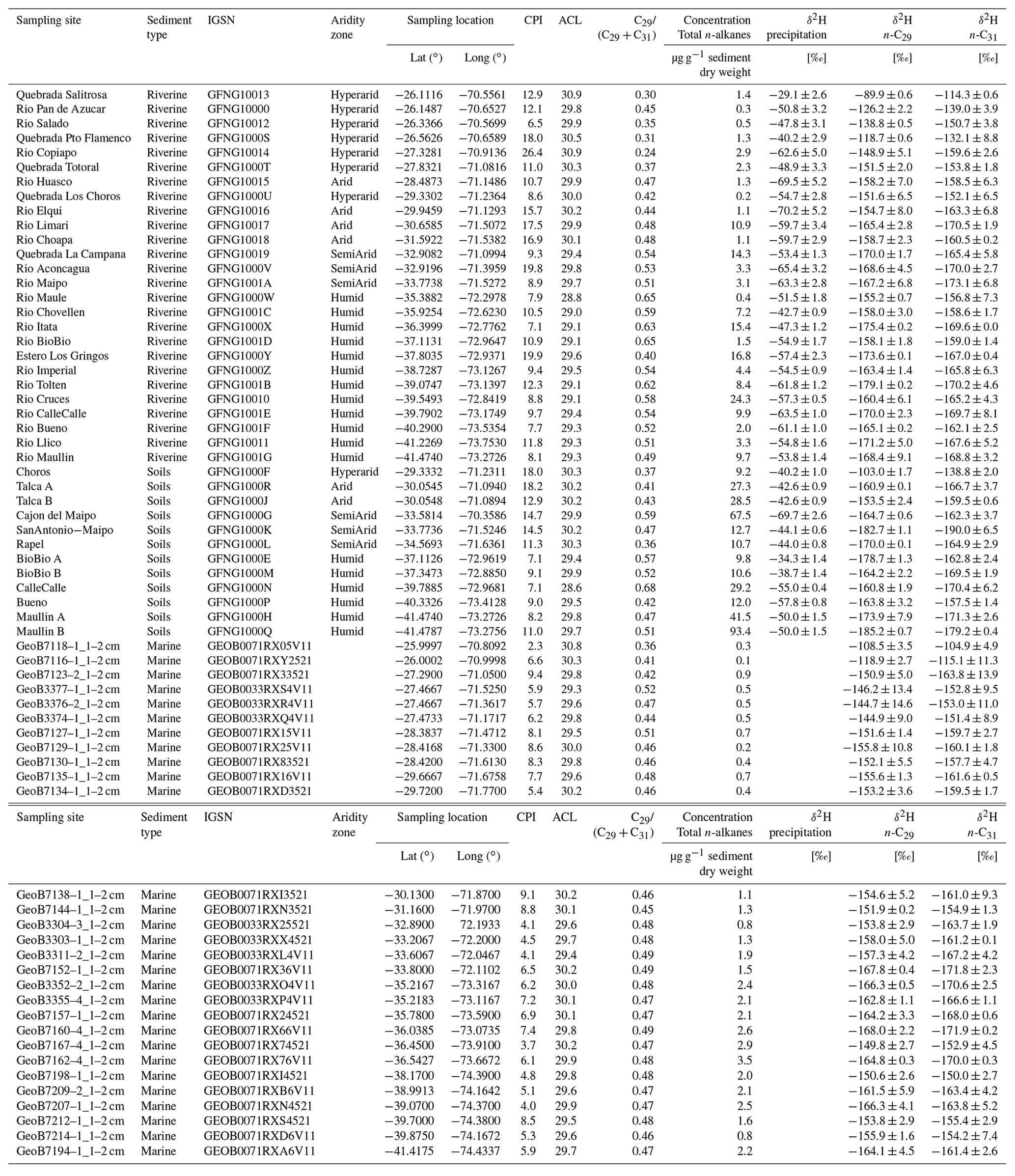
Here we study a gradient from hyperarid to humid along Chile, using soils, river sediments, and marine surface sediments (Fig. 1). During March–April 2019 we sampled topsoils (upper 5 cm, n=12) and riverbed sediments (n=26) from catchments draining to the Pacific Ocean. Three small sub-catchments nested in three of the major catchments were also sampled. Marine core-top sediments (1–2 cm core depth, 29 sites, Table 1) were provided by the MARUM core repository. Marine samples used in this study were recovered during expeditions SO-102 and SO-156 of the RV SONNE using a multicorer (Hebbeln, 1995, 2001).

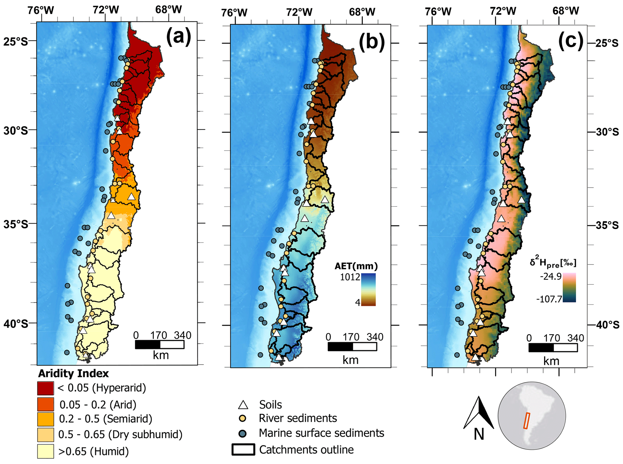
Figure 1 Maps of climatic conditions and sampling locations along the studied gradient. (a) Aridity index (dimensionless quantity) with sampling locations and studied catchments. Aridity index data are from the Global Aridity Index and Potential Evapotranspiration Climate Database v3 of Trabucco and Zomer (2022), and aridity zone classification follows the classification proposed by UNEP (1997). (b) Long-term (1958–2015) mean annual actual evapotranspiration (AET; mm yr⁻¹) from the TerraClimate dataset of Abatzoglou et al. (2018). (c) Mean annual hydrogen isotopic composition of precipitation (δ²H_pre, in ‰), from The Online Isotopes in Precipitation Calculator, version 3.1.

2.2 Analytical methods

2.2.1 Sample preparation

Prior to extraction of the organic compounds, samples from river and soil sediment were dried for 48 h in an oven at 60 ^∘C. Any visible plant material was carefully extracted using steel tweezers, and the samples were sieved to < 32 µm. Marine surface sediments were freeze-dried for 48 h and homogenized using an agate mortar.

Table 1 n-alkanes concentration, n-alkanes indices, δ²H_pre and δ²H_wax.

2.2.2 Lipid extraction and chromatography

Organic lipids were extracted from ∼ 20 g of sediment and purified using the manual solid phase extraction (SPE) procedure described by Rach et al. (2020). In brief, a Dionex Accelerated Solvent Extraction system (ASE 350, ThermoFisher Scientific) using a dichloromethane (DCM) : methanol (MeOH) mixture (9:1, $v/v$) at 100 ^∘C, 103 bar pressure with two extraction cycles (20 min static time) was used to extract total lipid extracts (TLE). These were collected in a combusted glass vial and then completely evaporated under a stream of nitrogen. All samples were spiked with 10 µg of an internal standard (5α-androstane) and the TLE was separated into aliphatic, aromatic, and alcohol $/$ fatty acid fractions by SPE in 8 mL glass columns filled with 2 g silica gel using Hexane, Hexane:DCM (1:1), and DCM : Methanol (1:1) as solvents. The aliphatic fraction was desulfurized by elution through activated copper powder, and then additionally cleaned over silver nitrate-coated silica gel.

Identification and quantification of n-alkanes were performed on an Agilent 7890A gas chromatograph (GC) coupled to a flame ionization detector (FID) and to an Agilent 5975C mass spectrometer (MS). The GC was equipped with a 30 m Agilent DB-5MS UI column (0.25 µm film thickness, 25 mm diameter). We used the internal standard to normalize the peak areas of the n-alkanes in the chromatogram. The internal standard was spiked into the sample after extracting the TLE from the sediments, but before performing the separation of the TLE through SPE. This allowed us to compare the relative abundance of the n-alkanes in different samples, while accounting for any losses that may have occurred during SPE. Quantification results were normalized to their initial dry weight and are reported as µg g⁻¹ dry weight. The uncertainty of the δ²H_wax values was calculated using the standard deviation between the duplicate measurements of each sample.

2.2.3 Hydrogen isotope analysis

Stable hydrogen isotope ratios (δ²H) from the n-alkanes were measured in the separated aliphatic fractions using a Trace GC 1310 (ThermoFisher Scientific) connected to a Delta V plus Isotope Ratio Mass Spectrometer (IRMS) (ThermoFisher Scientific). The GC was equipped with a 30 m Agilent DB-5MS UI column (0.25 µm film thickness, 25 mm diameter). n-alkane δ²H values were determined by duplicate measurements. We followed the same GC oven program as described by Rach et al. (2014). The H${}_{\mathrm{3}}^{+}$ factor was measured before each sequence and averaged 2.82 ± 0.14 mV (n=6) over a period of 5 weeks. To correct and transfer to the VSMOW scale, an n-alkane standard-mix A6 (n-C₁₆ to n-C₃₀) with known δ²H values obtained from A. Schimmelmann (Indiana University) was measured before and after the samples.

2.3 n-Alkane indices

To assess variations in the n-alkane distributions along the Chilean gradient, we calculated the carbon preference index (CPI) and the average chain length (ACL) indices. The CPI measures the relative abundances of odd- vs. even-numbered n-alkanes, using the concentrations of odd- and even-numbered n-alkane chains from n-C₂₅ to n-C₃₅ following Marzi et al. (1993):

$$\begin{array}{}\text{(1)}& \mathrm{CPI}={\displaystyle \frac{\begin{array}{c}\left({\mathrm{C}}_{\mathrm{25}}+{\mathrm{C}}_{\mathrm{27}}+{\mathrm{C}}_{\mathrm{29}}+{\mathrm{C}}_{\mathrm{31}}+{\mathrm{C}}_{\mathrm{33}}\right)\\ +\left({\mathrm{C}}_{\mathrm{27}}+{\mathrm{C}}_{\mathrm{29}}+{\mathrm{C}}_{\mathrm{31}}+{\mathrm{C}}_{\mathrm{33}}+{\mathrm{C}}_{\mathrm{35}}\right)\end{array}}{\mathrm{2}\left({\mathrm{C}}_{\mathrm{26}}+{\mathrm{C}}_{\mathrm{28}}+{\mathrm{C}}_{\mathrm{30}}+{\mathrm{C}}_{\mathrm{32}}+{\mathrm{C}}_{\mathrm{34}}\right).}}\end{array}$$

The ACL value is the weighted average of the various carbon chain lengths in a sample:

$$\begin{array}{}\text{(2)}& \mathrm{ACL}={\displaystyle \frac{\begin{array}{c}\left(\mathrm{25}\times {\mathrm{C}}_{\mathrm{25}}\right)+\left(\mathrm{27}\times {\mathrm{C}}_{\mathrm{27}}\right)+\left(\mathrm{29}\times {\mathrm{C}}_{\mathrm{29}}\right)\\ +\left(\mathrm{31}\times {\mathrm{C}}_{\mathrm{31}}\right)+\left(\mathrm{33}\times {\mathrm{C}}_{\mathrm{33}}\right)+\left(\mathrm{35}\times {\mathrm{C}}_{\mathrm{35}}\right)\end{array}}{{\mathrm{C}}_{\mathrm{25}}+{\mathrm{C}}_{\mathrm{27}}+{\mathrm{C}}_{\mathrm{29}}+{\mathrm{C}}_{\mathrm{31}}+{\mathrm{C}}_{\mathrm{33}}+{\mathrm{C}}_{\mathrm{35}.}}}\end{array}$$

2.4 Global δ²H_wax data compilation

The compiled dataset is accessible from the Gaviria-Lugo et al. (2023) data publication and can be correspondently used and cited. We used the previously published δ²H_wax datasets of soils and lake sediments of Ladd et al. (2021) and Chen et al. (2022), but significantly expanded these compilations with newer datasets reporting δ²H_wax for both n-C₂₉ and n-C₃₁. In total, our compilation includes data from 26 peer-reviewed publications, with 750 and 663 δ²H_wax values for n-C₂₉ and n-C₃₁, respectively (Table S1 in the Supplement).

2.5 Remote sensing data and GIS methods

2.5.1 δ²H of precipitation

δ²H_pre was extracted from the grids produced by Bowen and Revenaugh (2003), which are publicly available at the Online Isotopes in Precipitation Calculator webpage (OIPC, The Online Isotopes in Precipitation Calculator, version 3.1). We used the raster grid of annual averaged δ²H_pre data from the OIPC to calculate the δ²H_pre values for each location in our study area and from the global compilation. The raster grid data were provided at a resolution of ∼ 9 km, with each pixel corresponding to an area of ∼ 81 km². To assess the accuracy of OIPC δ²H_pre values at our sampling sites, we compare the values predicted by the OIPC, extracted on a monthly basis, with a dataset comprising 923 measured data points of δ²H_pre. This dataset was obtained from the International Atomic Energy Agency (IAEA/WMO, 2023), collected as part of the Global Network of Isotopes in Precipitation (GNIP) program at nine long-term monitoring stations located along the different aridity zones of continental Chile.

2.5.2 Climatic parameters

Hydrological variables were obtained from the TerraClimate dataset (Abatzoglou et al., 2018) as long-term annual averages for the period between 1958 and 2019 at ∼ 4.5 km spatial resolution, with each pixel representing ∼ 20 km². Variables obtained from the dataset were mean annual precipitation (MAP), actual evapotranspiration (AET), soil moisture (SM), actual vapor pressure (VAP), and vapor pressure deficit (VPD); the last two were used to derive relative humidity (RH) using Eq. (3):

$$\begin{array}{}\text{(3)}& \mathrm{RH}\left(\mathit{\%}\right)={\displaystyle \frac{\mathrm{VAP}}{\mathrm{VAP}+\mathrm{VPD}}}\times \mathrm{100}.\end{array}$$

The TerraClimate dataset was accessed and analyzed using the cloud computing capabilities publicly available via Google Earth Engine. Aridity index (AIdx) data were accessed from the Consultative Group of the International Agricultural Research Consortium for Spatial Information (CGIARCSI) Global-Aridity Index dataset (Trabucco and Zomer, 2022) that integrates aridity over the period 1970–2000 at a resolution of ∼ 1 km, with each pixel corresponding to ∼ 1 km². The WorldClim dataset (Fick and Hijmans, 2017) was used to derive the mean annual temperature (MAT) and annual average of daily maximum temperature (MaxT), based on data from 1970–2000 with a resolution of ∼ 1 km, corresponding to ∼ 1 km² per pixel.

2.5.3 Vegetation cover

Fractional land cover data were obtained from Collection 2 of the Copernicus Global Land Cover layers (Buchhorn et al., 2020) via Google Earth Engine. We extracted mean values for the fraction of trees, shrubs, grasses, crops, and barren land for the period 2015–2019 at a 100 m resolution, with each pixel representing 0.01 km². We used land cover fractions of vegetation obtained for each site to derive values of the fraction of herbaceous vegetation and woody vegetation. To derive the woody fraction of the vegetation, we summed the values of trees and shrubs land cover and divided this sum by the sum of all the vegetation fractions (trees, shrubs, grasses, crops). The values of the herbaceous fraction of the vegetation were derived summing the values of grasses and crops and dividing this sum by the sum of all the vegetation fractions (trees, shrubs, grasses, crops).

2.5.4 Spatial analysis

Catchments were defined upstream of the sampling points of river sediments using the drainagebasins function from the MATLAB-based software TopoToolbox 2 (Schwanghart and Scherler, 2014). The digital elevation model (DEM) used for the drainage basin definition in this study was the freely available Copernicus WorldDEM with a resolution of 30 m (Fahrland et al., 2020). For each catchment area, we calculated a mean value of δ²H_pre, the climatic parameters, and vegetation cover fractions (Table S6) of all grid cells within the catchment. Soil samples were considered as points, and in this case we extracted the values of δ²H_pre, the climatic parameters, and vegetation cover fractions from the pixel containing the sampling point (Table S6 in the Supplement). For the compiled global dataset, all soil samples were also treated as points, and drainage basins were defined for lake sediment samples using the same procedure as for the Chilean river samples. Values for δ²H_pre and all climatic parameters were retrieved using the same procedures and the same sources as for our sampling sites in Chile (Table S1).

2.6 Statistical and mathematical methods

2.6.1 δ²H_wax vs. δ²H_pre regression and analysis of residuals

Using the R programming language, we conducted a linear regression between the global compilation of δ²H_wax values and their corresponding δ²H_pre values retrieved from the OIPC. This global regression serves as an indicator of the expected relationship between δ²H_wax and δ²H_pre. To assess the influence of fractionation processes on δ²H_wax along the Chilean gradient, we calculated the residuals between measured δ²H_wax and predictions from the global regression for our sampling sites. As δ²H_pre is assumed to be the primary determinant of δ²H_wax, any substantial deviations from the global regression may suggest the presence of additional fractionation processes.

2.6.2 Statistical test of the differences between medians of groups (Kruskal–Wallis test)

The Kruskal–Wallis test was used to statistically test the hypothesis that the median δ²H_wax values are similar among the different aridity zones and sediment types. This non-parametric test does not make any assumptions about the distribution of the data, and using the median instead of the mean helps to avoid errors induced by outliers in the data. If the p value of the test is < 0.05, then the null hypothesis must be rejected, indicating a statistically significant difference between the medians of the groups (Kruskal and Wallis, 1952). We performed the test using the function kruskal.test of the stats package version 4.2.1 from the R programming language (R Core Team, 2022).

2.6.3 Leaf wax hydrogen isotope fractionation

We calculated the difference between δ²H_pre values as source water and δ²H_wax values to assess the climatic parameters that control δ²H_wax along the gradient. This difference is referred to as the “net or apparent fractionation”, as it encompasses several fractionation processes, such as the evaporation and enrichment of soil water, the enrichment of leaf water through transpiration, and the biosynthesis of lipids (Sessions et al., 1999; Smith and Freeman, 2006; Farquhar et al., 2007; Sachse et al., 2012). We used the isotopic fractionation factor (α) instead of the apparent fractionation in permil (ε ‰) to derive accurate regressions and to be mathematically consistent according to the theory of compositional data analysis (Aitchison, 1982, 1986), but reported all values as ε (in ‰) for the sake of comparison with other studies. Since α is the ratio of the isotopic composition of two substances, it enables application of the log-ratio approach when studying the factors affecting fractionation. Using log ratios is the preferred approach to yield mathematically and statistically robust regression models for compositional data (Aitchison, 1982, 1986; Ramisch et al., 2018; Weltje et al., 2015).

To obtain the fractionation factor α, delta values were transformed back to isotopic ratios from the permil scale using Eqs. (4) and (5). The apparent fractionation is related to the isotopic fractionation factor through Eq. (6). For comparison with existing literature data, apparent fractionation values in permil can be obtained multiplying Eq. (6) by 1000.

$$\begin{array}{}\text{(4)}& {\displaystyle }{\mathit{\delta }}_i={\displaystyle \frac{{\mathit{\delta }}_i\mathrm{‰}}{\mathrm{1000}}}\text{(5)}& {\displaystyle }{\mathit{\alpha }}_{\mathrm{wax}/\mathrm{pre}}={\displaystyle \frac{{\mathit{\delta }}_{\mathrm{wax}}+\mathrm{1}}{{\mathit{\delta }}_{\mathrm{pre}}+\mathrm{1}}}\text{(6)}& {\displaystyle }{\mathit{\epsilon }}_{\mathrm{wax}/\mathrm{pre}}={\mathit{\alpha }}_{\mathrm{wax}/\mathrm{pre}}-\mathrm{1}\end{array}$$

To explore the environmental controls on fractionation, we fitted ordinary least squares regression models between the natural log of the isotopic fractionation factor and the natural log of the environmental parameters of interest. The type of linear model obtained is represented by Eq. (7). To back-transform this type of model from the log space to the original space, we applied an exponential function to both sides of Eq. (7) to obtain a model in the form of Eq. (8):

$$\begin{array}{}\text{(7)}& {\displaystyle }\ln \left({\mathit{\alpha }}_{\mathrm{wax}/\mathrm{pre}}\right)=a\cdot \ln \left(X\right)+b\text{(8)}& {\displaystyle }{\mathit{\alpha }}_{\mathrm{wax}/\mathrm{pre}}=X^a\cdot e^b\end{array}$$

2.6.4 Soil and leaf water enrichment models

To mechanistically understand how evapotranspirative ²H enrichment with respect to source water regulates δ²H_wax, it is advantageous to model the effect of this process considering its two primary components: (1) soil water ²H enrichment due to evaporation and (2) leaf water ²H enrichment due to transpiration. To model soil water ²H enrichment we used a simplified Craig–Gordon model based on the modifications of Gat (1995) and followed the parameterization of Smith and Freeman (2006). The soil water is treated as a through-flow reservoir at hydrologic and isotopic steady state. The ²H enrichment (Δ²H_SW) is predicted for each site using Eq. (9) based on relative humidity (RH), and the ratio between precipitation (MAP) and evaporated soil water (SEv). RH and MAP data come from the retrieved values for each site (Sect. 2.5.2; Table S6). The equilibrium isotope fractionation factor between vapor and liquid (ε^*) is calculated as a function of temperature following the empirical relation derived by Horita and Wesolowski (1994).

$$\begin{array}{}\text{(9)}& {\mathrm{\Delta }}^{\mathrm{2}}{H}_{\mathrm{SW}}={\displaystyle \frac{\left(\mathrm{1}-\mathrm{RH}\right)\times \left({\mathit{\epsilon }}^{*}+\mathrm{12.5}\right)}{\mathrm{RH}+\left[\left(\mathrm{1}-\mathrm{RH}\right)\times \left(\frac{\mathrm{MAP}}{\mathrm{SEv}}\right)\right]}}\end{array}$$

The value of SEv is derived from AET from Eq. (10), in which the soil evaporation factor (f_e) reflects the contribution of soil evaporation to AET. This factor f_e varies along the aridity gradient.

$$\begin{array}{}\text{(10)}& \mathrm{SEv}=f_{\mathrm{e}}\times \mathrm{AET}\end{array}$$

It is known that the contribution of (soil) evaporation to AET is higher in arid regions compared to humid regions (Lawrence et al., 2007; Zhang et al., 2016). According to Lehmann et al. (2019), in arid regions, only 13 % of the precipitated water is shielded from evaporation, and this percentage decreases to 2.3 % in hyperarid regions. Based on these values, which consider evaporation not only from soils but also from water bodies, we assume conservative f_e values of 0.8 for arid regions and 0.9 for hyperarid regions. The present study does not model the contribution of soil evaporation to ²H enrichment in humid regions, as it is typically less significant than transpiration in such regions (Schlesinger and Jasechko, 2014; Zhang et al., 2016).

Leaf water enrichment is modeled using the Péclet modified Craig–Gordon model proposed by Kahmen et al. (2011) for δ¹⁸O values, adjusted for δ²H values as in Rach et al. (2017). Based on Eq. (11), this model first estimates leaf water ²H enrichment (Δ²H_LW) considering ε^* (defined as for the soil evaporation model), the kinetic isotope fractionation during water vapor diffusion from the leaf intercellular air space to the atmosphere (ε_k), the ²H enrichment of water vapor relative to source water (Δ²H_WV), and the ratio of atmospheric vapor pressure and leaf internal vapor pressure ($e_{\mathrm{a}}/e_{\mathrm{i}}$).

$$\begin{array}{}\text{(11)}& {\mathrm{\Delta }}^{\mathrm{2}}{\mathrm{H}}_{\mathrm{LW}}={\mathit{\epsilon }}^{*}+{\mathit{\epsilon }}_{\mathrm{k}}+\left({\mathrm{\Delta }}^{\mathrm{2}}{H}_{\mathrm{WV}}-{\mathit{\epsilon }}_k\right){\displaystyle \frac{e_{\mathrm{a}}}{e_{\mathrm{i}}}}\end{array}$$

As in Eq. (12), ε_k is dependent on two parameters that are considered constant: leaf boundary layer resistance (r_b=1 mol m⁻² s⁻¹) and stomatal conductance (g_s=0.1 mol⁻¹ m² s) which is formulated as stomatal resistance $r_{\mathrm{s}}=\mathrm{1}/g_{\mathrm{s}}$.

$$\begin{array}{}\text{(12)}& {\mathit{\epsilon }}_k={\displaystyle \frac{\left(\mathrm{16.4}\times r_{\mathrm{s}}\right)+\left(\mathrm{10.9}\times r_{\mathrm{b}}\right)}{r_{\mathrm{s}}+r_{\mathrm{b}}}}\end{array}$$

The magnitude of Δ²H_WV (Eq. 13) is considered the same as ε^*, as demonstrated by long-term observations in temperate regions (Jacob and Sonntag, 1991).

$$\begin{array}{}\text{(13)}& {\mathrm{\Delta }}^{\mathrm{2}}{\mathrm{H}}_{\mathrm{WV}}=-{\mathit{\epsilon }}^{*}\end{array}$$

Leaf internal vapor pressure (e_i; Eq. 14) is dependent on leaf temperature (T_leaf), which is considered to be the same as air temperature (T_air) over decadal timescales of sedimentary integration (Rach et al., 2017). Saturation vapor pressure (e_sat; Eq. 15) depends on T_air and atmospheric pressure (e_atm) at each site. With the value of e_sat, we calculate the atmospheric vapor pressure (e_a; Eq. 16).

$$\begin{array}{}\text{(14)}& {\displaystyle }{e}_{\mathrm{i}}=\mathrm{6.13753}\times \exp \left(T_{\mathrm{air}}\times {\displaystyle \frac{\mathrm{18.564}-\frac{T_{\mathrm{air}}}{\mathrm{254.4}}}{T_{\mathrm{air}}+\mathrm{255.57}}}\right)\text{(15)}& {\displaystyle }{e}_{\mathrm{sat}}={\displaystyle \frac{\mathrm{1.0007}+\mathrm{3.46}\times e_{\mathrm{atm}}}{\mathrm{1}\mathrm{000}\mathrm{000}}}\times \mathrm{6.1121}\times \exp \left({\displaystyle \frac{\mathrm{17.502}\times T_{\mathrm{air}}}{\mathrm{240.97}+T_{\mathrm{air}}}}\right)\text{(16)}& {\displaystyle }{e}_{\mathrm{a}}={\displaystyle \frac{\mathrm{RH}}{\mathrm{100}}}\times e_{\mathrm{sat}}\end{array}$$

The final component of the model involves the utilization of the Péclet number (℘) to adjust for physiological factors that can influence leaf water enrichment. The calculation of ℘ entails the preliminary estimation of the transpirational water flux (Tr; Eq. 17) and water diffusivity (D_iff; Eq. 18).

$$\begin{array}{}\text{(17)}& {\displaystyle }\mathrm{Tr}={\displaystyle \frac{e_{\mathrm{i}}+e_{\mathrm{a}}}{r_{\mathrm{b}}+r_{\mathrm{s}}}}\text{(18)}& {\displaystyle }{D}_{\mathrm{iff}}={\mathrm{10}}^{-\mathrm{8}}\exp \left(-\mathrm{0.7}+{\displaystyle \frac{\mathrm{1729}}{T\left[K\right]}}-{\displaystyle \frac{\mathrm{586977}}{T{\left[K\right]}^{\mathrm{2}}}}\right)\end{array}$$

For the calculation of ℘ (Eq. 19), path length (L_M=15 mm) and the molar concentration of water ($C=\mathrm{5.56}\times {\mathrm{10}}^{\mathrm{4}}$ mol m⁻³) are considered constant, following Kahmen et al. (2011). After obtaining ℘, the final Peclét corrected leaf water ²H enrichment values (Δ²H_LWP; Eq. 20) can be calculated.

$$\begin{array}{}\text{(19)}& {\displaystyle }\mathrm{\wp }={\displaystyle \frac{L_{\mathrm{M}}\times Tr}{C\times D_{\mathrm{iff}}}}\text{(20)}& {\displaystyle }{\mathrm{\Delta }}^{\mathrm{2}}{H}_{\mathrm{LWP}}={\displaystyle \frac{{\mathrm{\Delta }}^{\mathrm{2}}{H}_{\mathrm{LW}}\left(\mathrm{1}-e^{-\mathrm{\wp }}\right)}{\mathrm{\wp }}}\end{array}$$

3 Results

3.1 Concentration and distribution of leaf wax n-alkanes along the Chilean aridity gradient

3.1.1 Concentration and distribution of n-alkanes in river sediments and soils

In both soils and riverine sediments, n-alkane distributions exhibited a strong predominance of odd over even chain length n-alkanes with a CPI between 6.5 and 26.4 (Table 1). Total concentrations of n-alkanes in riverine sediments ranged from 0.2 µg g⁻¹ sediment dry weight (dw) to 24.3 µg g⁻¹ dw. Total concentrations of n-alkanes in soils ranged from 9.2 to 93.4 µg g⁻¹ dw. Concentrations of n-alkanes both in riverine sediments and in soil samples were lowest in the hyperarid zone and highest in the humid zone (Table 1). ACL varied along the aridity gradient (Table 1), ranging from 28.6 to 30.9; the highest ACL values were found in the hyperarid zone and the lowest in the humid zone (Table 1). The most prevalent n-alkane homologues were n-C₃₁ and n-C₂₉. In the hyperarid and arid zones, n-C₃₁ was the most common, while in the semiarid and humid zones, n−C₂₉ predominated (Tables 1 and S4).

3.1.2 Concentration and distribution of n-alkanes in marine sediments

All 29 marine sediments analyzed presented odd over even chain length predominance with a CPI between 2.3 and 9.4 (Table 1). The n-alkane concentration was lowest (0.1 µg g⁻¹ dw) in sediments adjacent to the hyperarid zone and highest (3.5 µg g⁻¹ dw) in sediments adjacent to the humid zone (Table 1). In the marine sediments, the chain length distribution of the n-alkanes varied with an ACL ranging from 29.3 to 30.8 (Table 1). The highest ACL values were found in sediments adjacent to the hyperarid zone (30.8), but no clear trend with latitude was apparent in the ACL values of the marine sediments. The most abundant n-alkane homologue in the marine surface sediments studied was n-C₃₁, except for two samples in the hyperarid zone, where n-C₂₉ concentration was higher (Tables 1, S4).

3.2 δ²H_wax values of river, soil, and marine sediments

3.2.1 δ²H_wax values in river sediments and soils

The δ²H_wax values of the n-C₂₉ and n-C₃₁ homologues varied from −90 ‰ to −185 ‰, and from −114 ‰ to −190 ‰ respectively (Table 1). The mean δ²H_wax values from n-C₂₉ in the hyperarid and arid zones were found to be 8 ‰ higher than the mean values from n-C₃₁, while in the humid zone, the mean δ²H_wax values from n-C₂₉ were 1 ‰ lower compared to those from n-C₃₁.

We examined the relationship between the measured δ²H_wax and δ²H_pre derived from the OIPC (Fig. 2a, c). We found that n-C₂₉ and n-C₃₁ δ²H_wax values from our Chilean river sediments show a positive correlation with δ²H_pre (δ²H n-C₂₉: R²=0.43, p<0.001; n-C₃₁: R² = 0.52, p<0.001) (Table 2), while δ²H_wax from Chilean soils show no significant correlation with δ²H_pre (n-C₂₉:R²=0.06, p=0.41; n-C₃₁: R²=0.04, p=0.56) (Table 2). Analyzing river and soil δ²H_wax together vs. δ²H_pre we found a low value, yet still with a statistically significant correlation (n-C₂₉: R²=0.14, p=0.02; n-C₃₁: R²=0.14, p=0.02) (Table 2).

Table 2 Statistical parameters of the linear regressions between δ²H_pre and δ²H_wax. The regressions obtained are of the type y = Intercept + Slope × x, df indicates the number of degrees of freedom from the fitted linear model and F is the F-statistic number.

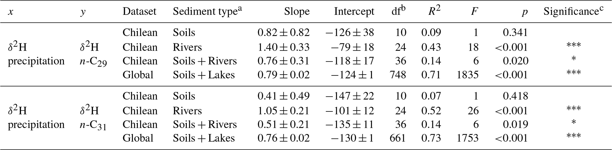
^a Sediment type refers to the sample set that was used for the regressions; enables comparison of the relationships on the different spatial scales. ^b df refers to degrees of freedom of the regression model, for this case it is the number of samples minus 2. ^c The number of asterisks indicates the significance of the regression. If a p value is greater than 0.05 there are no asterisks. If a p value is between 0.05 and 0.01, it is represented with one asterisk (^*). If a p value is between 0.01 and 0.001, it is represented with two asterisks (${}^{**}$). If a p value is less than 0.001, it is represented with three asterisks (${}^{***}$).

For the global compiled dataset, combining the lakes and soils data, we found a strong significant correlation between δ²H_wax and δ²H_pre (n-C₂₉: R²=0.71, p<0.001; n-C₃₁: R²=0.73, p<0.001) (Table 2, Fig. 2a, c). Chilean δ²H_wax values from the humid, semiarid, and arid zones generally follow the linear relationship between δ²H_wax and δ²H_pre established by the global dataset (Fig. 2a, c), while δ²H_wax values from the hyperarid zone exhibit a noticeable departure from the global linear relationship between δ²H_wax and δ²H_pre (Fig. 2a, c).

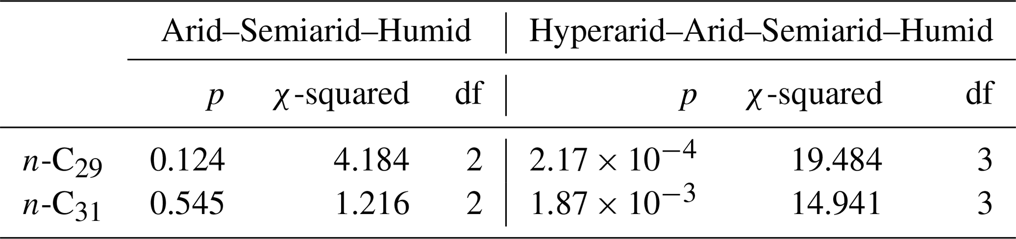
From our measured samples, we used δ²H_wax values from river and soil samples to calculate residuals, following the methodology described in Sect. 2.6.1. δ²H_wax value residuals, from n-C₂₉ and n-C₃₁, were highest in samples from the hyperarid zone (Fig. 2b, d and Table S5) and decreased with increasing humidity. n-C₂₉ mean residual values ranged from 32 ‰ in the hyperarid zone to −3 ‰ in the humid zone, while n-C₃₁ residuals varied from 23 ‰ in the hyperarid zone to 4 ‰ in the humid zone. Residuals from n-C₂₉ and n-C₃₁ for the humid, semiarid, and arid zones showed no significant differences (Kruskal–Wallis test, Sect. 2.6.2; n-C₂₉: p=0.125; n-C₃₁: p=0.545; Table 3). When residuals from the hyperarid zone were analyzed together with the residuals from the other zones, the Kruskal–Wallis test indicated the existence of a significant difference among them (n-C₂₉: p<0.001; n-C₃₁: p<0.002; Table 3).

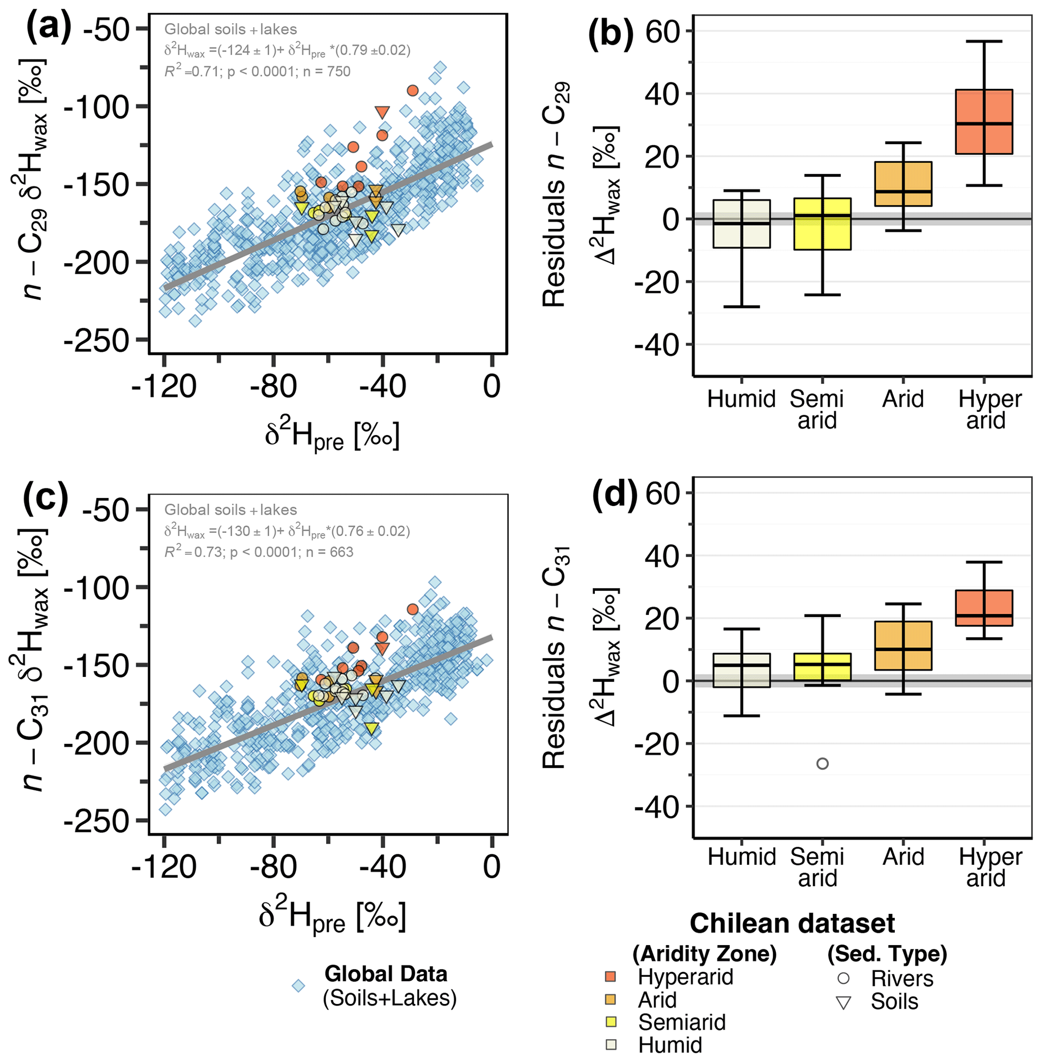
Figure 2 (a, c) δ²H_wax values from n-C₂₉ and n-C₃₁ homologues vs. δ²H_pre. Inverted triangles represent Chilean soil samples, circles represent Chilean river sediment samples. The blue diamonds represent δ²H_wax from a global compilation of previously published data from soils and lake surface sediments (Table S1). δ²H_pre data for both the Chilean locations and the global compilation dataset are derived from OIPC (Bowen and Revenaugh, 2003). The gray line in the plot illustrates the linear relationship between δ²H_wax and δ²H_pre for the global dataset, as indicated by the equation and regression parameters annotated within the plot. (b, d) Boxplots of the calculated residuals from the Chilean sediments (soils + river sediments) with respect to the global regression. The aridity zone classification follows the classification proposed by UNEP (1997).

3.2.2 δ²H_wax values in marine sediments

δ²H_wax values of n-C₂₉ and n-C₃₁ in marine sediments varied from −108 ‰ to −168 ‰, and from −105 ‰ to −172 ‰, respectively (Table 1). For both n-C₂₉ and n-C₃₁, δ²H_wax values were highest in marine sediments adjacent to the continental hyperarid zone and lowest in sediments adjacent to the continental humid zone. δ²H_wax values from n-C₂₉ were on average 4 ‰ higher compared to values from n-C₃₁ along the gradient (Table 1).

Table 3 Results of Kruskal–Wallis tests performed to evaluate the difference in residual values across different aridity zones.

3.3 Apparent hydrogen isotope fractionation along the Chilean gradient

Apparent fractionation values (${\mathit{\epsilon }}_{\mathrm{wax}/\mathrm{pre}}$) varied from −63 ‰ to −150 ‰, and from −88 ‰ to −153 ‰ for the n-C₂₉ and n-C₃₁ homologues, respectively (Table S6). Both soil and river sediments exhibited higher ${\mathit{\epsilon }}_{\mathrm{wax}/\mathrm{pre}}$ values in the hyperarid zone (${\mathit{\epsilon }}_{\mathrm{wax}/\mathrm{pre}}$ n-C${}_{\mathrm{29}}=-\mathrm{63}$ ‰; ${\mathit{\epsilon }}_{\mathrm{wax}/\mathrm{pre}}$ n-C${}_{\mathrm{31}}=-\mathrm{88}$ ‰). In general, ${\mathit{\epsilon }}_{\mathrm{wax}/\mathrm{pre}}$ values were increasingly negative with increasing humidity.

We found significant non-linear relationships between ${\mathit{\epsilon }}_{\mathrm{wax}/\mathrm{pre}}$ and water-climate parameters, i.e., AET, MAP, SM, RH, and aridity index (Table S7). AET showed the strongest correlation with ${\mathit{\epsilon }}_{\mathrm{wax}/\mathrm{pre}}$ (river sediments n-C₂₉: R²=0.72, p<0.0001; river sediments n-C₃₁: R²=0.61, p<0.0001) (Fig. 3, Table S7). Parameters associated solely with temperature (i.e., mean annual temperature, mean annual max daily temperature) showed no correlation with ${\mathit{\epsilon }}_{\mathrm{wax}/\mathrm{pre}}$ (Table S7). The ${\mathit{\epsilon }}_{\mathrm{wax}/\mathrm{pre}}$ values obtained from river samples were more strongly correlated with the climatic parameters than the ${\mathit{\epsilon }}_{\mathrm{wax}/\mathrm{pre}}$ values from soils (Table S7).

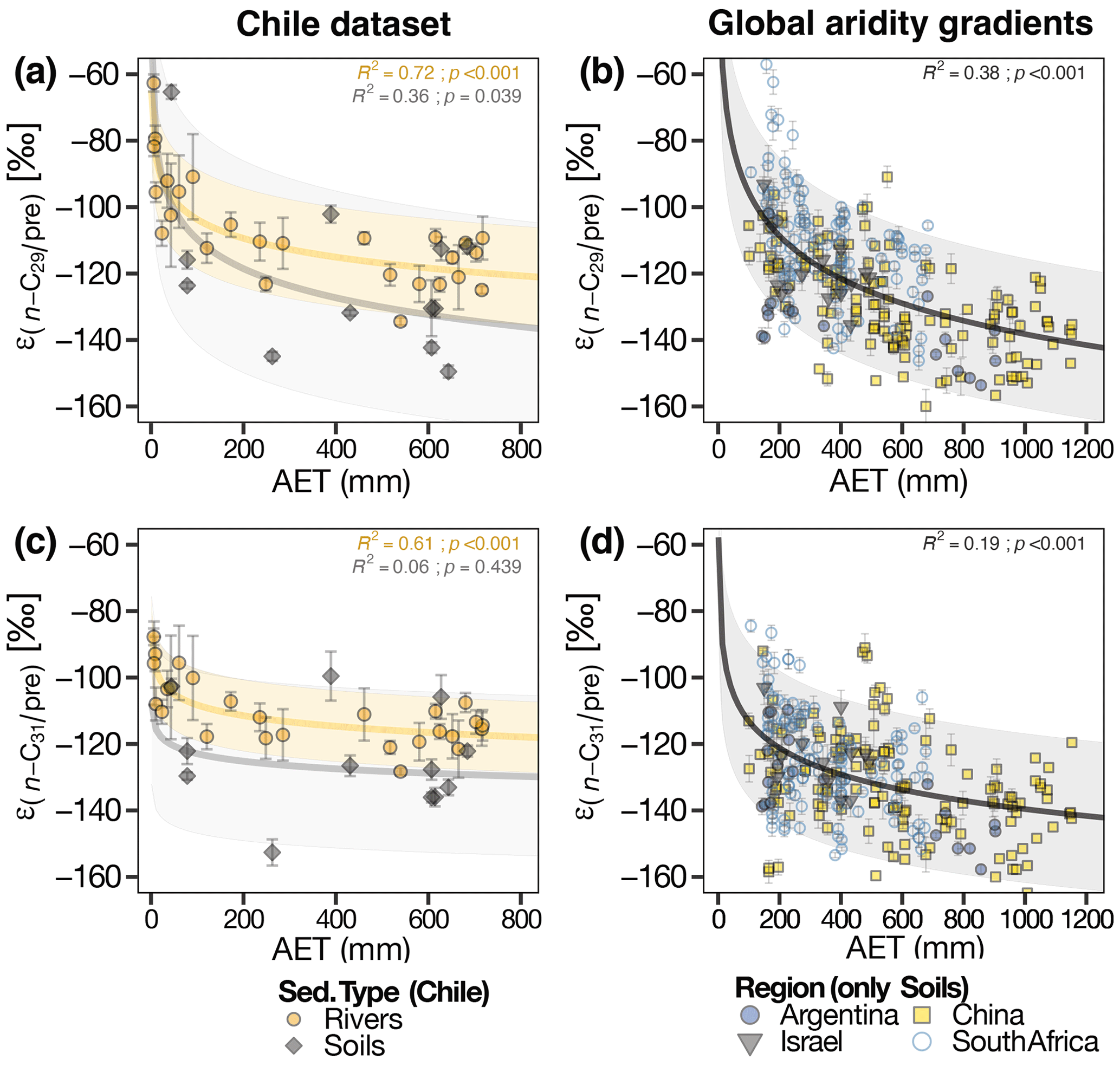
Figure 3 ${\mathit{\epsilon }}_{\mathrm{wax}/\mathrm{pre}}$ vs. AET (actual evapotranspiration). (a, c) Chilean soils and river sediments. Shaded gray area represents 95 % CI of the model fitted to the soil data, shaded yellow area represents 95 % CI of the model fitted to the river sediments. (b, d) Soils from aridity gradients of Argentina (Tuthorn et al., 2015), China (Rao et al., 2009; Li et al., 2019; Lu et al., 2020), Israel (Goldsmith et al., 2019), and South Africa (Herrmann et al., 2017; Strobel et al., 2020). Shaded gray area represents 95 % CI of the model fitted to the full dataset.

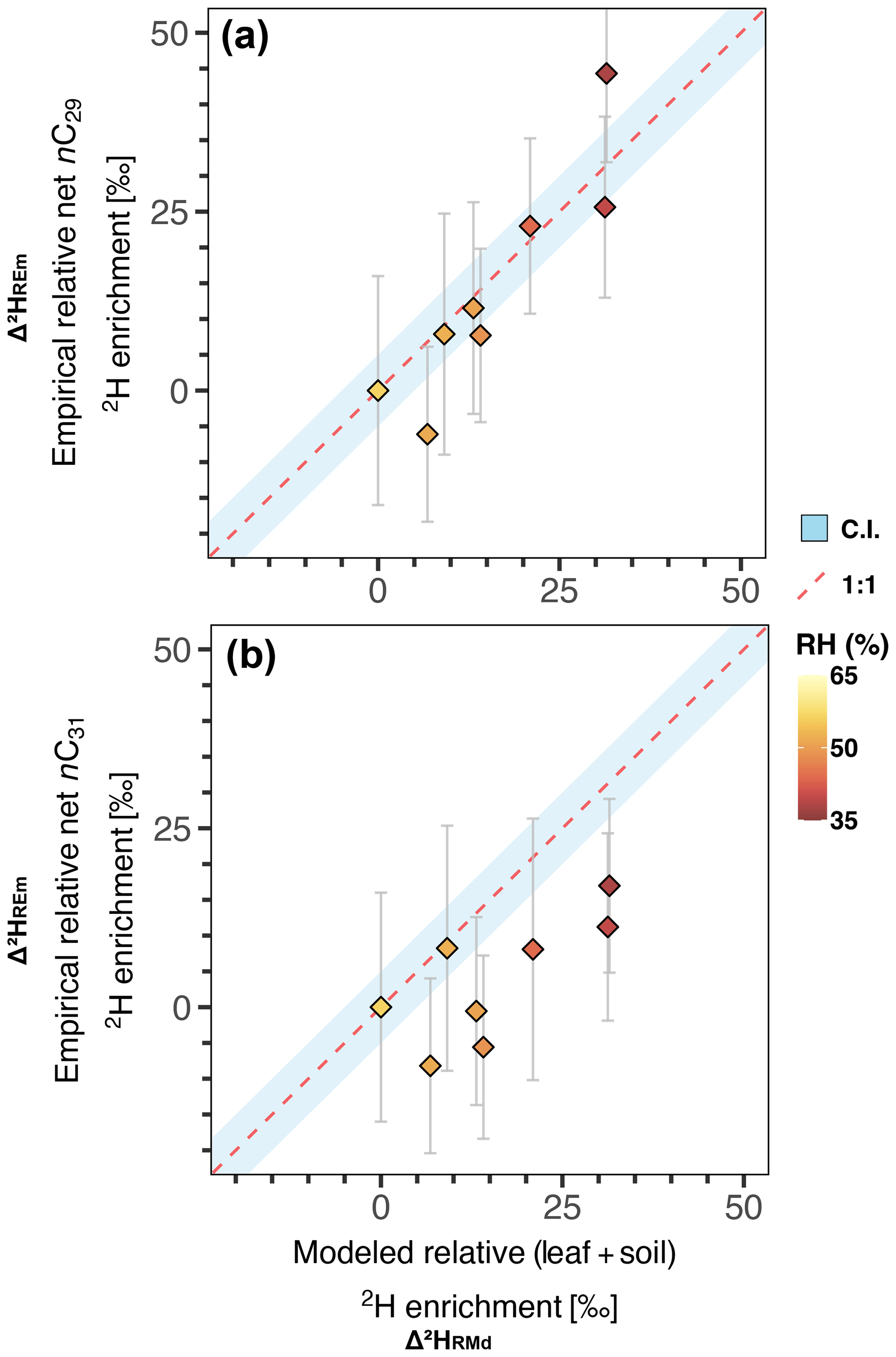
Figure 4 Δ²H_REm vs. Δ²H_RMd for the catchments of the hyperarid zone. The dashed red line represents a 1:1 line; an analytical uncertainty range of 5 ‰ is used to represent the confidence interval (shaded blue area). Markers are color-coded by relative humidity (RH). (a) Results obtained for the n-C₂₉ homologue. (b) Results obtained for the n-C₃₁ homologue.

4 Discussion

4.1 Causes of δ²H_wax variability in sediments and soils along the Chilean aridity gradient

4.1.1 Assessment of the OIPC δ²H_pre values along the aridity gradient

Analyzing the drivers of δ²H_wax values requires robust data on δ²H_pre. Since no long-term time series are available for the exact locations of our sampling sites, we rely on interpolated data generated by the OIPC (see above). Thus, a first factor to consider in our interpretations is the accuracy of the δ²H_pre values derived from the OIPC. The OIPC provides long-term estimates of modern (post-1950) mean δ²H_pre, at monthly and annual grids, which may differ from the δ²H_pre measured at a particular site on a short-term basis. The longer-term estimates from the OIPC are advantageous for our study, as soils and river sediments can integrate leaf waxes over spans of several decades to centuries (Huang et al., 1996; Douglas et al., 2014; Vonk et al., 2019). Consequently, we expect that δ²H_pre values from OIPC are the more relevant predictors for our δ²H_wax values. The OIPC model is based on data from GNIP stations (Bowen and Revenaugh, 2003), of which nine fall within continental Chile and can be used as a validation dataset. They range from the humid zone to the border between the arid and hyperarid zones and include a total of 923 monthly precipitation datapoints between 1964 and 2017 (Table S3). We find a significant linear relationship (R²=0.53, p<0.0001) between the δ²H_pre predicted by OIPC and measured δ²H_pre (Fig. S1a). Grouping by month and taking the long-term average of the measured δ²H_pre values, we found that the correlation is stronger (R²=0.80, p<0.0001) (Fig. S1b). Although there are uncertainties associated with the predicted OIPC δ²H_pre values, particularly in regions with sparse GNIP station coverage, the results presented above validate the use of OIPC δ²H_pre values across the studied aridity gradient in Chile.

4.1.2 δ²H_pre values control δ²H_wax values in the humid to arid zone

In the humid and semiarid zones of Chile δ²H_pre values are the main factor determining δ²H_wax values. Our results show that δ²H_wax values from soils and river sediments in the humid and semiarid zones of Chile generally follow the global linear relationship between δ²H_wax and δ²H_pre. This is confirmed through the residuals analysis (Fig. 2b, d) and is in accordance with the findings of previous studies in humid and semiarid regions (Feakins et al., 2016; Hou et al., 2008; Sachse et al., 2006; Tipple and Pagani, 2013; Tuthorn et al., 2015; Häggi et al., 2016; Bertassoli et al., 2022). Therefore, we suggest that δ²H_wax is primarily controlled by δ²H_pre in the humid and semiarid zones of Chile.

In the arid zone of Chile, δ²H_wax values show a slight deviation from the global regression between δ²H_wax and δ²H_pre (Fig. 2b, c). However, this deviation is not statistically significant when compared to the deviation of δ²H_wax values from the humid and semiarid zones of Chile (Table 3). As a result, the net or apparent fractionation between water source and lipid biomarker (${\mathit{\epsilon }}_{\mathrm{wax}/\mathrm{pre}}$) is not significantly different in the arid zone when compared to humid and semiarid zones. Although previous studies have found that δ²H_wax values in arid zones are consistently higher due to changes in ${\mathit{\epsilon }}_{\mathrm{wax}/\mathrm{pre}}$ (Douglas et al., 2012; Feakins and Sessions, 2010; Polissar and Freeman, 2010), we cannot resolve a statistically significant difference between the arid zone, the humid zone, and semiarid zone (Fig. 2b, c, Table 3). This might be because earlier studies including arid zones focused on lakes draining small areas or exclusively analyzed soil and plant samples (Douglas et al., 2012; Feakins and Sessions, 2010; Polissar and Freeman, 2010; Schwab et al., 2015). Our study analyzed only two soil samples from the arid zone, which may not be a complete representation of the whole δ²H_wax variability. It is important to note that δ²H_wax values are significantly more variable in soils than in river sediments in all climate zones (as discussed in Sect. 4.4). Therefore, further sampling at smaller subcatchments or at the soil scale is necessary to confidently test whether δ²H_wax largely reflects δ²H_pre in the arid zone.

4.1.3 Controls on δ²H_wax variability in the hyperarid zone

δ²H_wax values in the hyperarid zone of Chile are influenced by additional factors beyond δ²H_pre values, as suggested by the Kruskal–Wallis test results (Table 3) and the deviation of δ²H_wax values from the global linear relationship between δ²H_wax and δ²H_pre (Fig. 2a, c). Along aridity gradients, climatic parameters such as evapotranspiration, RH, and aridity itself have been identified as key factors that exert control over ${\mathit{\epsilon }}_{\mathrm{wax}/\mathrm{pre}}$ values (Douglas et al., 2012; Polissar and Freeman, 2010; Schwab et al., 2015; Herrmann et al., 2017; Li et al., 2019). The mechanism behind this control is rooted in the impact that these climatic parameters have on soil water enrichment and leaf water enrichment (Gat, 1996; Smith and Freeman, 2006; Kahmen et al., 2013a). To determine the factors controlling ${\mathit{\epsilon }}_{\mathrm{wax}/\mathrm{pre}}$ along the Chilean aridity gradient, we conducted a regression analysis as outlined in Sect. 2.6.3. This analysis examined ${\mathit{\epsilon }}_{\mathrm{wax}/\mathrm{pre}}$ against three broad categories of climatic factors: temperature, water content, and water fluxes. Temperature was evaluated based on maximum daily temperature (MaxT) and mean annual temperature (MAT). Water content in the soil and atmosphere was evaluated through relative humidity (RH), soil moisture (SM), and aridity index (AIdx). Water fluxes were analyzed through actual/net evapotranspiration (AET) and mean annual precipitation (MAP). To further validate our findings, we used data from four previously published aridity gradients to determine if the observed trends are characteristic of strong aridity gradients globally, or simply a feature of the Chilean dataset. We selected four regions with the most pronounced aridity gradients in our compilation (Table S2), comprising data from soils from Argentina (Tuthorn et al., 2015), China (Rao et al., 2009; Li et al., 2019; Lu et al., 2020), Israel (Goldsmith et al., 2019), and South Africa (Herrmann et al., 2017; Strobel et al., 2020). To maintain the rigor of our analysis, we adopted a cautious approach and excluded publications that contained marked altitude gradients within the four selected regions, thereby eliminating the potentially confounding effect of elevation.

Our regression analysis indicates that no significant relationship exists between MAT or MaxT and ${\mathit{\epsilon }}_{\mathrm{wax}/\mathrm{pre}}$ (Table S7), which is consistent with mechanistic models of leaf water enrichment, which demonstrate a low sensitivity to variations in temperature (Farquhar and Gan, 2003; Kahmen et al., 2011; Rach et al., 2017). Furthermore, field studies in climatic transects along South Africa from Strobel et al. (2020) also found no significant correlation between temperature and ${\mathit{\epsilon }}_{\mathrm{wax}/\mathrm{pre}}$. Similarly, along an aridity gradient in Argentina, Tuthorn et al. (2015) showed that RH exerts a greater control than temperature on the magnitude of ²H enrichment in leaf waxes. Thus, the narrow MAT range of 8–17 ^∘C along our study area is expected to have minimal impact on leaf water enrichment and consequently on ${\mathit{\epsilon }}_{\mathrm{wax}/\mathrm{pre}}$.

The significant correlations that we found between ${\mathit{\epsilon }}_{\mathrm{wax}/\mathrm{pre}}$ and variables linked to water content and water fluxes (Table S7) highlight the influence of hydrological conditions on ${\mathit{\epsilon }}_{\mathrm{wax}/\mathrm{pre}}$ values. Results from a principal component analysis (Fig. S2) demonstrate that hydrological variables are correlated, contributing to 69% of the total variance observed. This confirms the synchronized variation of these parameters, due to the hydrological cycle's water balance, and to some degree, their autocorrelation (Douglas et al., 2012). Similarly, all hydrological variables are strongly correlated with ${\mathit{\epsilon }}_{\mathrm{wax}/\mathrm{pre}}$ in our study, but AET exhibits the highest correlation (Fig. 3, Table S7). Hence, we suggest that in the hyperarid zone of Chile, δ²H_wax values are strongly controlled by evapotranspirative processes, in addition to δ²H_pre values.

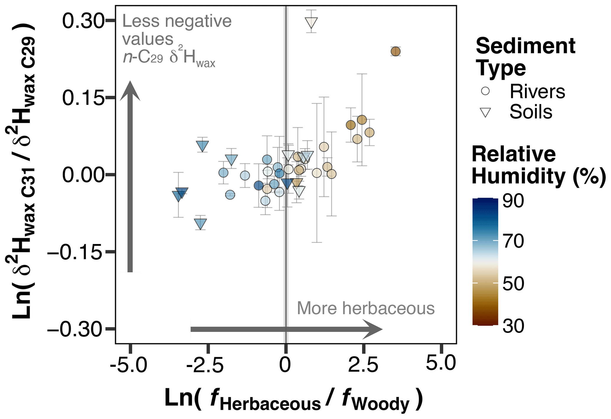
Figure 5 Plot of log ratio between n-C₃₁ δ²H_wax and n-C₂₉ δ²H_wax vs. the log ratio between the fraction of herbaceous plants and fraction of woody plants. The fractions of herbaceous and woody vegetation were obtained following the methods described in Sect. 2.5.3. The vegetation cover is derived at the scale of the catchment area for river sediment samples and at the maximum resolution of the pixel (100 m × 100 m) for soil samples. Vegetation cover fraction data are from Buchhorn et al. (2020).

4.1.4 Soil and leaf water enrichment modeling in the hyperarid zone

We modeled the ²H enrichment in soil and leaf water of river samples in the hyperarid zone using Eqs. (9) and (20). By comparing the model results with the enrichment measured in our samples, while holding vegetation parameters constant, we can isolate the contribution of climatic factors to the changes in ${\mathit{\epsilon }}_{\mathrm{wax}/\mathrm{pre}}$ along the gradient. Equations (9) and (20) produce net soil (Δ²H_SW) and net leaf water enrichment (Δ²H_LWP) values, respectively, for each sample. To make the modeled Δ²H_SW and Δ²H_LWP values comparable with empirical ${\mathit{\epsilon }}_{\mathrm{wax}/\mathrm{pre}}$ values, we standardize the values of each catchment relative to the values obtained for the southernmost catchment of the hyperarid zone (Los Choros) (Table S8). From the standardization of the ${\mathit{\epsilon }}_{\mathrm{wax}/\mathrm{pre}}$ values we obtain an empirical relative net ²H enrichment for each catchment (Δ²H_REm). The standardization of Δ²H_SW and Δ²H_LWP yields a relative Δ²H_SW and a relative Δ²H_LWP, the sum of which yields a modeled relative ²H enrichment for each catchment (Δ²H_RMd) (Table S8). The progressive aridification trend toward the north offers an opportunity to evaluate the consistency between Δ²H_REm and Δ²H_RMd in response to aridity. Additionally, this approach eliminates the uncertainty surrounding the absolute value of biosynthetic fractionation, which would otherwise be a requirement for comparison of the Δ²H_SW and Δ²H_LWP against ${\mathit{\epsilon }}_{\mathrm{wax}/\mathrm{pre}}$.

Our modeling approach was able to reproduce well the empirical enrichment measured in n-C₂₉, but the enrichment measured in n-C₃₁ was overestimated (Fig. 4a, b). Despite the high uncertainties propagated into the empirical relative enrichment values, the agreement between modeled and empirical values for n-C₂₉ supports the hypothesis that evapotranspiration processes play a significant role in the fractionation of hydrogen isotopes in the hyperarid zone of Chile. Although for n-C₃₁ most of the empirical enrichment is reproduced within uncertainty, there is a clear overestimation of the enrichment by the model (Fig. 4b). The model overestimation for n-C₃₁ indicates that changes in climatic conditions alone do not account for all the variability in the magnitude of the enrichment. Some residual variability can be caused by vegetation effects that generate a differential enrichment in n-C₂₉ and n-C₃₁ among different plant types; this is further discussed in Sect. 4.2.

4.2 Aridity highlights δ²H_wax differences among n-C₂₉ and n-C₃₁ n-alkanes

In arid sites dominated by herbaceous vegetation, n-C₂₉ consistently exhibited higher δ²H_wax values compared to n-C₃₁ (Fig. 5, Table S6). This suggests a differential response of the homologues to evapotranspirative processes, which can be attributed to the plant sources from which they originate. Woody plants like trees and shrubs generally yield higher concentrations of n-C₂₉ than n-C₃₁, and herbaceous plants like grasses and forbs tend to produce higher concentrations of n-C₃₁ than n-C₂₉ (Kuhn et al., 2010; Zech et al., 2010; Duan and He, 2011; Howard et al., 2018; Bliedtner et al., 2018). Herbaceous plants possess different strategies to cope with aridity, including the development of smaller leaves and the use of CAM photosynthesis. Also, in desert ecosystems, herbaceous plants generally have greater rooting depths in comparison to woody plants like shrubs, which gives them access to water sources less enriched in ²H than surficial soil water (Ehleringer et al., 1991; Gibson, 1998; Gibbens and Lenz, 2001; Herrera, 2009; Feakins and Sessions, 2010; Kirschner et al., 2021). Additionally, greenhouse experiments have demonstrated that grasses use a mixture of enriched leaf water and less enriched soil water for biosynthesis (Kahmen et al., 2013a). Furthermore, plant physiology, biochemistry, or even the timing of leaf flush can have a significant impact on δ²H_wax (Bi et al., 2005; Liu et al., 2006; Smith and Freeman, 2006; Hou et al., 2007; Liu and Yang, 2008; Sachse et al., 2012; Tipple et al., 2013). Thus, it is possible that differences in δ²H_wax values of n-C₃₁ and n-C₂₉ homologues are the manifestation of distinct physiological and biochemical characteristics among different plant growth forms or particular plant species. In this study we focused on the level of plant growth forms due to the lack of plant species datasets at the scale of our study areas. However, it is important to note that within the same plant growth form, different plant species might exhibit distinct biosynthetic fractionation values and consequently affect δ²H_wax differently. The influence of both plant growth forms and plant species on sedimentary δ²H_wax over large scales is unclear, and more studies are needed to fully understand these relationships.

Notably, the differences in δ²H_wax values among homologues become significantly pronounced only under conditions of high aridity. These findings offer empirical evidence that disparities in δ²H_wax values between n-C₃₁ and n-C₂₉ homologues can potentially be utilized as a marker of specific vegetation and aridity conditions, such as the predominance of herbaceous plants under high aridity. Some studies noted and briefly discussed the divergence in δ²H_wax values from the n-C₂₉ and n-C₃₁ homologues (Garcin et al., 2012; Wang et al., 2013; Chen et al., 2022), but to our knowledge this has not been further analyzed. The results of this study suggest that differences between the homologues contain valuable information that could potentially be exploited as a proxy to indicate both aridity and the presence of herbaceous plants or possibly the presence of particular herbaceous species, but further research is needed to validate its application.

4.3 Non-linear relationship between ${\mathit{\epsilon }}_{\mathrm{wax}/\mathrm{pre}}$ and hydrological factors

The results of the regression analyses shown in Table S7 revealed that ${\mathit{\epsilon }}_{\mathrm{wax}/\mathrm{pre}}$ is non-linearly correlated with all the hydrological parameters studied. The ${\mathit{\epsilon }}_{\mathrm{wax}/\mathrm{pre}}$ values in Chilean soils exhibit non-linear correlations with hydrological factors. However, for Chilean soils, the only significant correlations between ${\mathit{\epsilon }}_{\mathrm{wax}/\mathrm{pre}}$ and climatic variables are with SM and AET, these correlations are observed only for the n-C₂₉ homologue. This likely reflects the low sample density of soils in our study, particularly in the arid and hyperarid regions. For river samples as well as for the four selected aridity gradients, the results show that all regressions against hydrological factors are significant and non-linear (Table S7). These results indicate that the non-linear relationship between ${\mathit{\epsilon }}_{\mathrm{wax}/\mathrm{pre}}$ and hydrological factors can be found on strong aridity gradients globally and is not merely an artifact of our data.

The non-linear relationship between enrichment and hydrological conditions can be modeled combining the leaf and soil water enrichment models explained in Sect. 2.6.4 of the methods. By parametrizing RH and MAP in terms of AET, Fig. 6 shows that the non-linear behavior can be reproduced when the model includes a component of soil evaporation (f_e>0). These modeling results support our findings and strengthen the idea that under high aridity, the relationship between ${\mathit{\epsilon }}_{\mathrm{wax}/\mathrm{pre}}$ and hydrological conditions is non-linear. Previous studies showed that ${\mathit{\epsilon }}_{\mathrm{wax}/\mathrm{pre}}$ is controlled by hydrological conditions (Hou et al., 2018; Smith and Freeman, 2006; Feakins and Sessions, 2010; Sachse et al., 2012; Douglas et al., 2012; Herrmann et al., 2017; Li et al., 2019; Lu et al., 2020), but most argue that the relationship between ${\mathit{\epsilon }}_{\mathrm{wax}/\mathrm{pre}}$ and the hydrological parameters is linear (Feakins and Sessions, 2010; Vogts et al., 2016; Herrmann et al., 2017; Li et al., 2019). By extensively including and analyzing samples from hyperarid regions, we demonstrate that ${\mathit{\epsilon }}_{\mathrm{wax}/\mathrm{pre}}$ behaves non-linearly along strong aridity gradients, as is also predicted by enrichment models incorporating both soil evaporation and leaf water transpiration (Fig. 6).

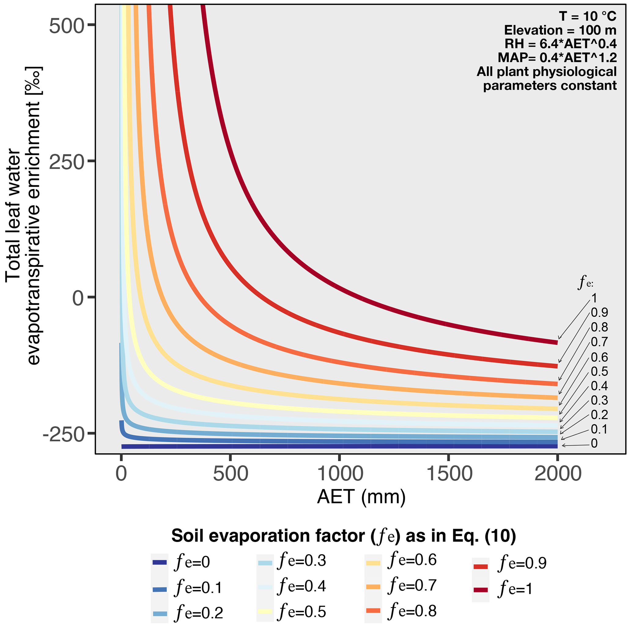
Figure 6 Modeled total leaf water evapotranspirative enrichment under varying AET, considering different soil evaporation factors (f_e). The f_e values are used to derive the soil evaporated water from AET as expressed in Eq. (10). The total evapotranspirative leaf water enrichment is obtained summing the results of Eqs. (9) and (20). To obtain the results for this figure, RH and MAP were parameterized as a function of AET (see Figs. S3 and S4), as such all the variation in the evapotranspirative enrichment is only driven by variation of AET.

4.3.1 δ²H_wax differences between soils, riverine and marine sediments

Analyzing the Chilean dataset at the differential spatial scales, we found that δ²H_pre values showed better correlation with δ²H_wax values from river sediments than from soils (Table 2). In addition, soil δ²H_wax values showed weaker correlations with all climatic variables than river δ²H_wax values. This suggests a larger effect of spatial averaging of the δ²H_wax values for the river sediment samples, as they integrate both vegetation and climatic variability over larger regions than soil samples. In support of this, Goldsmith et al. (2019) showed a significant reduction of variability via the early incorporation of the leaf waxes into soils, finding that variability of ${\mathit{\epsilon }}_{\mathrm{wax}/\mathrm{pre}}$ from soils is significantly lower than variability of ${\mathit{\epsilon }}_{\mathrm{wax}/\mathrm{pre}}$ from plants. In a similar manner, lake sediments exhibit lower ${\mathit{\epsilon }}_{\mathrm{wax}/\mathrm{pre}}$ variability than both plants (Sachse et al., 2006) and soils (Douglas et al., 2012) in their source areas.

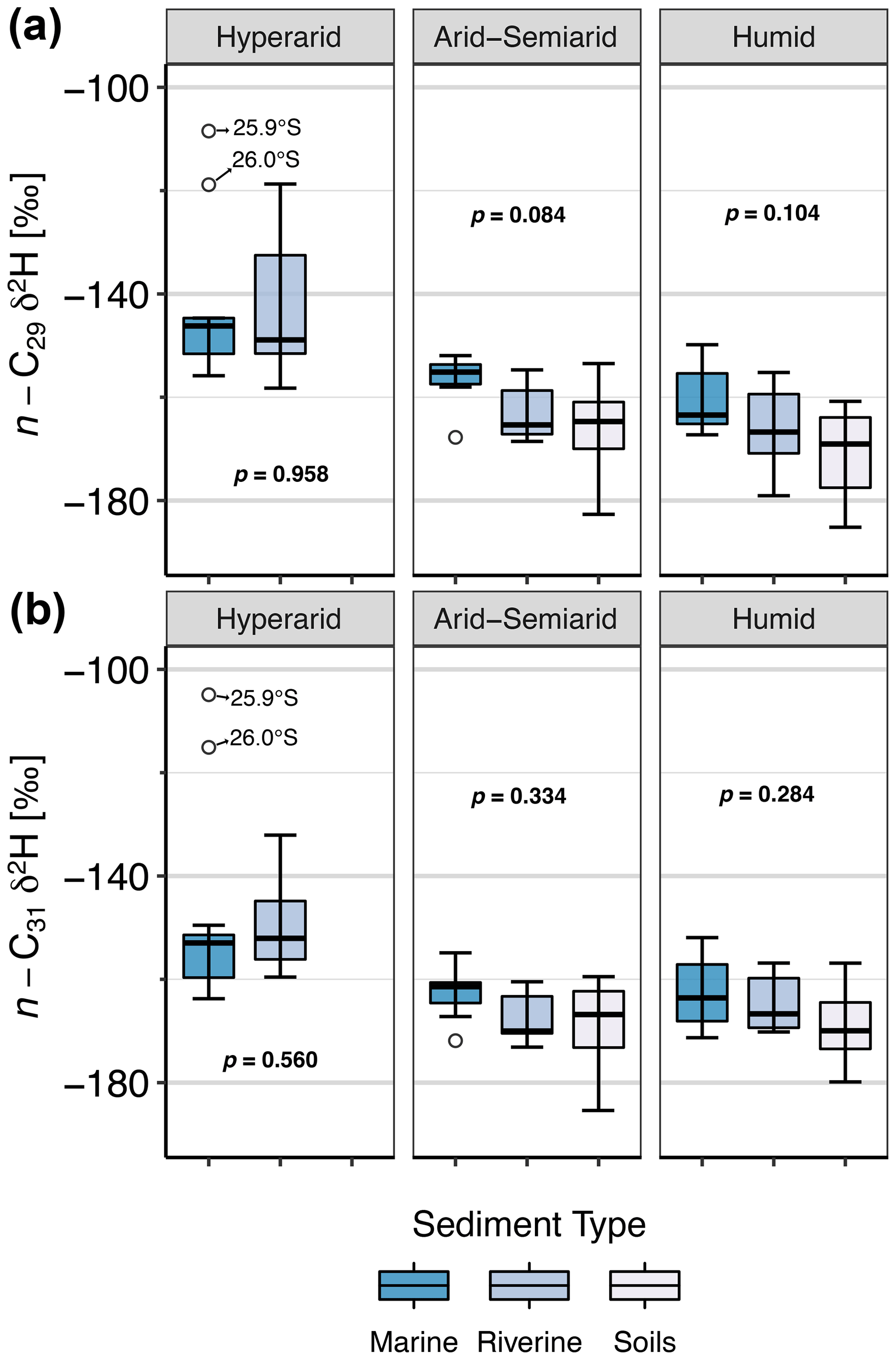
Figure 7 Boxplots of δ²H_wax in soils, rivers, and marine surface sediments, among the different climate zones. (a) Data for the n-C₂₉ homologue. (b) Data for the n-C₃₁ homologue. Arid and semiarid zones were grouped to overcome sample size limitations. In the hyperarid zone, only one soil sample was taken and therefore no box is shown.

Overall, the ranges of δ²H_wax values from soils, rivers, and marine sediments overlap (Fig. 7), but there are two notable outliers in marine sediments of the hyperarid zone (Fig. 7). These samples were taken adjacent to the Pan de Azúcar catchment at 25.9^∘ S (δ²H${}_{\mathrm{waxC}\mathrm{29}}=-\mathrm{108}$ ‰) and at 26.0^∘ S (δ²H${}_{\mathrm{waxC}\mathrm{29}}=-\mathrm{119}$ ‰) and have similar δ²H_wax values as continental samples from locations further south: the Quebrada Puerto Flamenco at 26.5^∘ S (δ²H${}_{\mathrm{waxC}\mathrm{29}}=-\mathrm{119}$ ‰) and Quebrada Salitrosa at 26.1^∘ S (δ²H${}_{\mathrm{waxC}\mathrm{29}}=-\mathrm{90}$ ‰), which are catchments with predominantly herbaceous vegetation that span small areas close to the coastline. This suggests that these catchments could be a source of sediments to the identified outliers.

We conducted a Kruskal–Wallis test (Sect. 2.6.2) to assess the presence of significant differences in δ²H_wax values among the soils, rivers, and marine sediments from the different aridity zones. Together with the two marine outliers (above), nested catchments (Quebrada Salitrosa, Quebrada La Campana, and Estero Los Gringos) were excluded from the analysis, as the major catchments that include them would be expected to contribute the δ²H_wax values transported to the marine sediments.

We find no statistical differences between mean δ²H_wax values of the sediment types within each climate zone (Fig. 7). This suggests that climatic signals recorded by δ²H_wax are effectively transported along the sedimentary systems. In general, marine sediments show the smallest range of δ²H_wax values in any given region, in line with the decrease in variability that follows an increase in integration area and integration time. Marine sediments are expected to integrate over larger areas and longer timescales than river sediments, acquiring sediments not only from near fluvial sources but also by eolian input or coast-parallel currents (Gagosian and Peltzer, 1986; Poynter et al., 1989; Bernhardt et al., 2016). Overall, our findings support the notion of consistent transport of δ²H_wax values from the continent to the adjacent marine sediments within each climate zone.

In Fig. 7, δ²H_wax values from marine sediments generally display higher δ²H_wax values in marine sediments in comparison to soils and river sediments. Although the difference between δ²H_wax values among the sediment types is not statistically significant, higher δ²H_wax values in marine sediments might be attributed to differences in sourcing and transport of the continental sediments. However, given the limited sample set of paired marine and river sediments in the arid region and the absence of statistically significant differences in δ²H_wax values between the sediment types, we consider further discussion would be too speculative at this point.

4.4 Implications for paleoclimate studies

Our results demonstrate the potential of δ²H_wax as a proxy for δ²H_pre in the humid-to-arid zones of Chile. We found that δ²H_wax values in marine sediments are consistent with those in river sediments and soils from the adjacent continent, supporting the use of marine sedimentary δ²H_wax as a tracer of continental δ²H_pre. However, our analysis also revealed that hyperaridity can cause strong ²H enrichment (i.e., smaller ${\mathit{\epsilon }}_{\mathrm{wax}/\mathrm{pre}}$ values) and non-linear relationships between hydrological variables and ${\mathit{\epsilon }}_{\mathrm{wax}/\mathrm{pre}}$. These findings suggest that δ²H_wax is highly sensitive to the onset of extreme aridity, while δ²H_wax values largely reflect δ²H_pre values in humid, semiarid, and arid settings. In hyperarid regions, the strong evapotranspirative effects on δ²H_wax could lead to an overestimation of δ²H_pre values, and consequently of hydrological changes, as also discussed by Hou et al. (2018). Because of this, it is crucial to consider the aridity states that an area may have experienced when using δ²H_wax as a paleoenvironmental proxy.

Furthermore, our analysis revealed differential responses of the n-C₂₉ and n-C₃₁ homologues under strong aridity conditions, likely due to different vegetation sources. We found that n-C₂₉ is more sensitive to aridity and exhibits higher δ²H_wax values relative to n-C₃₁ in sites with high aridity (Fig. 5). Similar findings have been reported in previous studies (Chen et al., 2022; Wang et al., 2013; Garcin et al., 2012). We found that the difference between δ²H_wax values in n-C₂₉ and n-C₃₁ is particularly pronounced in arid settings, especially where herbaceous vegetation dominates. This differential sensitivity could be useful in detecting the onset of high aridity, and thus could help avoid overestimation of hydrological changes. However, such an application requires additional information about the n-alkanes of the vegetation from the source areas.

In summary, along the Chilean humid-to-arid zones, our results support the use of δ²H_wax as a proxy for δ²H_pre and to study changes in paleohydrological conditions. However, with the onset of hyperaridity, δ²H_wax values can become decoupled from δ²H_pre and be controlled by evapotranspirative processes.

5 Conclusions

By analyzing soils, river sediments, and their marine counterparts along a strong aridity gradient in Chile, we tested the robustness with which the hydrogen isotope composition of leaf waxes (δ²H_wax) in soils and river sediments reflects modern climate conditions, and how accurately marine sediments preserve continental δ²H_wax values. We corroborate previous findings that in humid-to-arid zones, δ²H_wax values are largely controlled by δ²H_pre. However, in hyperarid zones, δ²H_wax values are additionally influenced by evapotranspirative enrichment, resulting in a non-linear relationship of δ²H_wax with hydrological variables. Using established models, we show that changes in RH, MAP and AET can explain most of the ²H enrichment for the n-C₂₉ homologue. The n-C₃₁ homologue is less sensitive to changes in hydrological conditions, suggesting that the δ²H_wax differences between the homologues reflect differences in leaf wax sources and their differential use of enriched leaf water and unenriched xylem water, as herbaceous vegetation is dominant under arid conditions. Further, the non-linearity that we found is particularly relevant in hyperarid zones, where small variations in hydrological parameters translate into large changes in δ²H_wax values. In paleoclimate studies, care must hence be taken when interpreting records in arid-to-hyperarid regions as records of δ²H_pre alone, since changes in δ²H_wax can become decoupled from changes in δ²H_pre and are rather driven by AET. The marine core-top samples that we analyzed reflect faithfully the continental δ²H_wax values from river sediments and soils along the entire aridity gradient, showing a land–ocean connectivity and preservation of terrestrial signals in the marine realm, even under the different hydrological regimes along the Chilean coast.