the Creative Commons Attribution 4.0 License.
the Creative Commons Attribution 4.0 License.
 | 27 Nov 2023
Imaging of the electrical activity in the root zone under limited-water-availability stress: a laboratory study for Vitis vinifera
Veronika Iván
Franco Meggio
Luca Peruzzo
Guillaume Blanchy
Chunwei Chou
Benedetto Ruperti
Giorgio Cassiani
Understanding root signals and their consequences for the whole plant physiology is one of the keys to tackling the water-saving challenge in agriculture. The implementation of water-saving irrigation strategies, such as the partial root zone drying (PRD) method, is part of a comprehensive approach to enhance water use efficiency. To reach this goal tools are needed for the evaluation of the root's and soil water dynamics in time and space. In controlled laboratory conditions, using a rhizotron built for geoelectrical tomography imaging, we monitored the spatio-temporal changes in soil electrical resistivity (ER) for more than a month corresponding to eight alternating water inputs cycles. Electrical resistivity tomography (ERT) was complemented with electrical current imaging (ECI) using plant-stem-induced electrical stimulation. To estimate soil water content in the rhizotron during the experiment, we incorporated Archie's law as a constitutive model. We demonstrated that under mild water stress conditions, it is practically impossible to spatially distinguish the limited-water-availability effects using ECI. We evidenced that the current source density spatial distribution varied during the course of the experiment with the transpiration demand but without any significant relationship to the soil water content changes. On the other hand, ERT showed spatial patterns associated with irrigation and, to a lesser degree, to RWU (root water uptake) and hydraulic redistribution. The interpretation of the geoelectrical imaging with respect to root activity was strengthened and correlated with indirect observations of the plant transpiration using a weight monitoring lysimeter and direct observation of the plant leaf gas exchanges.
- Article
(8199 KB) - Full-text XML
- BibTeX
- EndNote


In the context of water scarcity, agriculture needs to improve irrigation practices by reducing water inputs and selecting adequate species and, in the case of woody crops, the most efficient scion–rootstock combinations. In order to evaluate the efficacy of irrigation, it is necessary to develop tools capable of evaluating root functioning and quantifying root water uptake. The partial root zone drying (PRD) and RDI (regulated deficit irrigation) methods are part of an ensemble of deficit irrigation (DI) strategies that aim to improve water use efficiency. The PRD, for instance, consists of irrigating only one part of the root system of the same plant using a certain percentage of the potential evapotranspiration (ETp), usually inferior to the total water needed. The application of DI triggers a physiological response in the plant via a hormone called abscisic acid (ABA), which is produced in the roots and transmitted to the leaves to regulate the stomata closure, thus reducing water transpiration while keeping photosynthesis active, and finally leading to increased water use efficiency (as reviewed in Loveys et al., 2000; Davies et al., 2002). Notably, if there is adequate sap flow through the roots, the ABA signal is transmitted through the xylem to the leaf, as demonstrated by Dodd et al. (2008). According to Davies and Hartung (2004), it is proposed that plants subjected to partial PRD demonstrate improved performance compared to plants under deficit irrigation (DI) when an equal amount of water is applied. This is attributed to the ability of PRD to stimulate root growth and maintain consistent signalling of abscisic acid (ABA) to regulate shoot physiology. Davies and Hartung (2004) stated that the effects of PRD on plant growth, yielding, and functioning are quantitatively different from those of RDI. One of the advantages of PRD when operated properly is that plants sustained and even increased shoot and fruit turgor even though a reduced amount of water is applied to roots (Mingo et al., 2003). On the other hand, one of the disadvantages of RDI is that the entire root zone is allowed to dry out, the roots can become stressed and damaged, and, if not, rewetted can die and signalling may diminish. Conversely Fernández et al. (2006) stated that a PRD treatment has not always been found advantageous as compared to a companion regulated deficit irrigation (RDI) treatment and demonstrated it in a study on olive trees in which sap flow measurements, which reflected water use throughout the irrigation period, showed no evidence of stomatal conductance being more reduced in PRD than in RDI trees. Collins et al. (2009), in an experiment on the grapevine (Vitis vinifera L.) show that the response to PRD applied at 100 % ETc (crop evapotranspiration) and deficit irrigation applied at 65 % ETc was the same, increasing stomatal sensitivity to vapour pressure deficit and decreasing sap flow. According to Cai et al. (2022), while stomatal conductance is a significant aboveground hydraulic factor influencing water use in crops, it should not discount the role of belowground hydraulics, as changes in soil–plant hydraulic conductance have been found to drive stomatal closure (Abdalla et al., 2021). This highlights the crucial importance of studying electrical activity in the soil.
The plant's natural bioelectrical activity is necessary for its physiological processes. Plant scientists represent it by a water column where the ions move from bottom to top and vice versa due to gradients of water potentials. In their studies, Voytek et al. (2019) and Gibert et al. (2006) successfully linked the measurements of electrical potential in the ground and in the tree stem to the RWU (root water uptake) and sap flow respectively. The use of active methods such as electrical resistivity tomography (ERT) allows for spatial and temporal analysis of the subsoil. Recent advances in electrical tomography imaging, in particular reduced at the plant scale, show their effectiveness to measure changes in soil water content associated with the RWU (e.g. Cassiani et al., 2015, 2016; Mary et al., 2018). Note that the correlation between root water uptake and soil water content changes exists when averaged over a larger spatial scale than the scale at which soil moisture redistribution can compensate for local root activity. The determination of these spatial scales depends on the soil hydraulic properties. This correlation between root water uptake and changes in soil water content can also be influenced by the timescales in addition to spatial scales. The ability to discriminate between them relies on factors such as the soil hydraulic properties, rates of local water extraction, and the temporal dynamics of water redistribution in the soil (Anonymous Reviewer, 2023). Applications of geoelectrical methods to evaluate water use efficiency are increasing. Recently in an experimental citrus orchard, Consoli et al. (2017), Vanella et al. (2018), and Mary et al. (2019b) showed that the observed drying pattern resulting from an elevated evapotranspiration rate in the non-irrigated section of the root zone matches the root distribution in that area, while the observed wetting pattern arising from a decreased ER in the irrigated section of the root zone can be attributed to the irrigation itself.
However, processes occurring in the rhizosphere can affect the soil ER in various ways. Roots induce changes in the soil structure in terms of porosity and hydraulic conductivity which ultimately modify the water pathways and fluxes and thus the ER itself. Soil structure changes may have a relatively smaller effect on ER than root water uptake RWU, although this may differ for species with extensive root systems like woody species; this is further true during rainfall or irrigation considering water redistribution and channelling influenced by varying root anatomies and causing dynamic variations in ER. Stemflow channelling by roots is an example of how water from rain or irrigation can be driven to soil recharge by the root structure. Conversely, root uplift in agroforestry shows how water can move from the deeper layers to the top via the roots. Roots also affect the soil ER through the geochemical changes associated with root exudates and root symbiosis. At the interface between soil and roots, the chemical gradients and concentrations can drastically differ from those observed in the soil regions not affected by the roots. Although this can have a significant impact and be a valuable source of information, only a few studies have extended the ERT and the induced polarisation (IP) to observe these changes (Weigand, 2017; Weigand and Kemna, 2019; Tsukanov and Schwartz, 2020, 2021). As of today, the electrical behaviour of individual roots remains poorly understood, particularly with regard to their changes in type (from hair roots to fully lignified roots), space, time, and whether the root is active or not (Ehosioke et al., 2020).
The geophysical approach extends the scope of traditional methods to evaluate soil water content (SWC) using time-domain reflectometry (TDR) sensors and the calculation of RWU (Jackisch et al., 2020). In the field, the spatial resolution is controlled (in ERT or IP) by the arrangement of the electrodes and acquisition parameters (Uhlemann et al., 2018), while the temporal resolution is controlled by the time it takes to complete a full sequence measurement.
Rhizotrons are one of the earliest and most effective tools for studying root growth and functioning, both in the field and in the laboratory (Taylor et al., 1990). They are transparent boxes that allow the direct observation of the roots during plant growth and changes in soil conditions. Rhizotrons also provide valuable support in multidisciplinary studies, allowing other methods to be more easily and precisely deployed, so that their results are more reliably interpreted. For example, a load scale is often mounted in combination with the rhizotron in order to weigh the system, which allows inferring the quantity of water lost by the plant over time. This setup is inspired by the lysimeter and is widely adopted to measure the water balance of the soil–plant interactions. For example, in a rhizotron, Doussan and Garrigues (2019) use the light transmission 2D technique to infer root water uptake with respect to their genotypes.
The very few studies conducting geophysical tomography imaging in the laboratory using a rhizotron proved a certain efficiency in studying the interaction between soil physics and plant physiology for predicting plant response to environmental stresses (Weigand, 2017, 2019; Peruzzo et al., 2020). A rhizotron allows for high-resolution tomography by reducing the size, diameter, and spacing of the electrodes. The entire soil profile is easily accessible by placing electrodes on the side of the rhizotron, easing the depth resolution limitation inherent in surface-based geophysical methods usually used for field acquisition.
Although there is a good momentum for the use of geophysical methods applied to agronomy (Garré et al., 2021), a number of gaps still need to be addressed. All the indirect root effects on the soil ER affect the evaluation of the soil water content, sometimes making the interpretation of ERT to quantify RWU difficult (Ehosioke et al., 2020).
1.1 Current pathways in roots under water stress constraints
Current pathways in roots remain certainly the main unknown since there is a gap in techniques to measure it non-destructively (Ehosioke et al., 2020; Liu et al., 2021). The current pathways in roots are possibly linked to RWU. Lovisolo et al. (2016) describe in detail the flow of water from root water uptake and the processes occurring at the cell scale. In any case, root water uptake is not distributed equally over the whole root system, in part, due to heterogeneous soil conditions. For the same reason as soil saturation can change over time, RWU also varies in time. The concept of active roots has been previously employed by several authors (Frensch and Steudle, 1989; Doussan, 1998; Garrigues et al., 2006; Srayeddin and Doussan, 2009) to characterise the spatial variability in root water uptake. In this context, plants adapt by reducing radial conductivity in dry regions, enabling them to redirect their uptake towards wetter areas with higher soil conductivity. This mechanism allows plants to maintain a consistent rate of water uptake while sustaining higher plant water potentials. For active roots, root water uptake consists in a moving water from the root tip (which is usually much more electrically conductive due to high water conductivity at its proximity) in the radial direction via cellular routes (symplastic way) and between cells (apoplastic way) until it reaches the xylem, which transports it in the axial direction towards the upper part. Water flow can encounter resistances due to suberisation (conversion of the cell walls into cork tissue by development of suberin), which is naturally driven as a consequence of root growth (secondary roots are more suberised than primary roots), but it can also be the consequence of plant stress (Malavasi et al., 2016; Song et al., 2019). The process can cause reductions in water conductivity through the root system by limiting the permeability of the root tissue, thus leading to changes in the plant's ability to take up water. Aroca and Ruiz-Lozano (2012) describes in a generic manner the plant responses to drought stress. For the specific PRD case, there is a complex tradeoff induced by root suberisation between reducing radial flow (as a consequence of ABA signalling sent by the roots) to conserve water in the soil but keeping the axial flow active. This can be done for instance by adjusting the xylem vessels size and quantities. Although suberisation is usually a long-term process, studies show that PRD can promote and accelerate the process of suberisation in response to water limitation. Finally during PRD conditions we can also observe the transfer of water from the wet to the dry side through the roots (overnight) in a process called redistribution (Yan et al., 2020), which induces spatio-temporal variations in RWU that ultimately also influences electrical current pathways in roots.
A direct approach to analysing the active part of the root system consists of an injection of current stimuli into the plant stem. There is a variety of stem-based methods used in the literature with applications ranging from biomass estimation and root morphology to root physiology (root activity). At a single frequency, we distinguish between electrical capacitance measurements (ECM) methods which rely on capacitance measurements and are commonly used to study root systems at the plant scale and earth impedance method (EIM), which measures both capacitance and resistance. Capacitance represents the polarisation processes and measures the charges stored during the current flow. Both use the fact that the root can polarise at the soil–root interface and inside the root to infer direct root-related information such as dry and wet mass, surface area, etc.). A second group of methods, electrical impedance spectroscopy (EIS), uses a range of frequencies to capture the polarisation processes sensitive to the root physiology and anatomy. For a detailed description of the methods, the reader is invited to refer to (Ehosioke et al., 2020). The stem-based approach has been developed for years by plant physiologists, starting from the theory developed by Dalton (1995), who conceptualised the current pathways through the root xylem by an equivalent parallel resistance–capacitance circuit. The theory holds under the assumption that the current flows throughout the most conductive path and is held (thus inducing polarisation) by the root cell membranes before being released into the soil. Fine root connections and mycorrhiza facilitate the efficient transfer of injected current into the soil at contact points between roots and the soil, resulting in a distribution of current sources within the ground. Contrasting experimental results have challenged the relationship between root electrical capacitance and root traits in different crops, with studies highlighting the potential contribution of the stem, rather than the roots, to the overall measured root electrical capacitance and the occurrence of current leakage at the proximal part (Urban et al., 2011; Dietrich et al., 2018; Peruzzo et al., 2020).
Without being able yet to give suggestions about the electrical current pathway, recent advancements in the development of explicit RWU models, based on plant hydraulics, provide insights into how robustly capacitance models hold and under which conditions. We learnt, for instance, that at the root level, RWU models account for the anisotropy by separating the root hydraulic conductance into two terms i.e. axial and radial (Javaux et al., 2008; Couvreur et al., 2012). Figure 1 draws inspiration from the electrical circuit analogy of RWU proposed in previous works (Doussan et al., 1999; Manoli et al., 2014; Couvreur et al., 2012; Cai et al., 2022). In dry soil conditions, the primary part of the potential drop happens within the soil-to-root connection, while in wet soil conditions, the main portion of the potential drop is in the plant section. In dry soil, the gradient ) is higher than in wet soil. As the soil conductance gs is linked by the relationship between the transpiration rate over the Δψsoil, for the same evaporation rate, gs decreases when the soil dries out. The root axial water flow rates Qx (L3 T−1) and root radial water flow rates Qr (L3 T−1) can be solved analytically by solving the system of equations of Ohm's and Kirchhoff's laws (Couvreur et al., 2012).
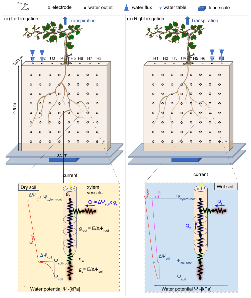
Figure 1Conceptual figure showing the position of the plant in the rhizotron. The water input was done alternatively from left (a) to right (b) via small holes on the top of the rhizotron (H1 to H8). The roots are free to grow on both sides of the rhizotron. The circles on the screening face show the locations of the electrodes. Two additional electrodes (needles) are used for the ECI: one for the stem injection and the other for the control soil injection next to the stem. The rhizotron is weighted by a central point load scale (PC60-30KG-C3, Flintec) mounted between two support plates in plexiglass. The line below describes the state of the art of hydraulic conductivity at a single root and the distinction between dry (c) and wet (d) soil. The figure draws inspiration from the electrical circuit analogy of RWU (root water uptake) proposed in previous works (Doussan et al., 1999; Manoli et al., 2014; Couvreur et al., 2012; Cai et al., 2022). In a recent article, Cai et al. (2022) schematised the gradient of potential ψsoil, ψsoil–root, and ψroot, along with the corresponding hydraulic conductances of the soil, the soil–root interface, and the root (represented as gs, gsr, and gr respectively), in response to high or low transpiration demand (E). Note that the soil–root interface and the xylem cell interfaces are seats of current polarisation due to the formation of the electrical double layer (EDL), described well in Tsukanov and Schwartz (2021).
The same applies to the stem-based methods as root hydraulic conductance and electrical conductivity are likely to vary conjointly. Up to now the relationship between root water content and root hydraulic conductivity with ER has not been firmly established. Many other parameters such as root function, age, water retention capacity, and transpiration rate in particular can affect the water flow as well as the current pathway of stem-based methods (Ehosioke et al., 2020).
Peruzzo et al. (2020) hypothesise that drought stress can also reduce electrical current leakage, wherein the current exiting the plant root at the proximal part is decreased, particularly for woody species. Furthermore, as expected, the frequency of the injected current plays an important role in the capacitance measured. At high frequencies, both the longitudinal conductivity and radial conductivity increase (Mancuso, 2012; Ehosioke et al., 2020), which can also cause current leakage problems (Gu et al., 2021). The measure of plant responses over multiple frequencies, a method called electrical impedance spectroscopy (EIS) is more time-consuming but more informative since different polarisation processes can manifest themselves in the signal (Ehosioke et al., 2020). The contrast of electrical resistivities between soil and roots plays a fundamental role as reported, e.g., by Cseresnyés et al. (2020). Gu et al. (2021) stated that the potential to directly quantify root traits under dry conditions is higher than under wet conditions and interpreted this as a result of the fact that the root electrical longitudinal conductivity is higher than that of the soil under dry conditions. The instrumentation and acquisition schemes used for impedance are also questionable and the optimal experimental setup of measurement remains to be determined (Postic and Doussan, 2016). The number and the position of the stem and the return electrodes are a cause of uncertainties (electrode contact resistance, etc.). Peruzzo et al. (2021), in a three-channel experiment, were able to provide direct access to the response of stem and soil, which ultimately allowed the decoupling of the root response. Evidence showed the presence of current leakage in herbaceous root systems, a significant contribution from the plant stem, and a minor impact from the soil.
Gu et al. (2021) stated that in addition to the traditional regression model used for predicting root traits using the impedance method, a forward model would help to illustrate the importance of these different factors. In order to cope with the main drawbacks of the impedance methods, we propose the so-called electrical current imaging (ECI) method, a physically based approach based on recovering the current density distribution instead of simply calculating the total resistance and/or capacitance. This method is also referred to as mise-à-la-masse (MALM) in the applied geophysics literature. The current imaging methods hold some promise to offer a first set of evidence about the current pathways: this is a popular technique adopted, e.g., by the neurosciences community, where the current density in the human brain correlates with diverse patterns of neural activity (Kamarajan et al., 2015). Peruzzo et al. (2020) applied it for plant root imaging with relative success, as the authors stated that all the current leaks at the plant's proximal part, i.e. at the shallowest contact of the plant stem with the soil. For the ECI approach, the Poisson's equation serves as a physical model for the electrical current flow. As current flow is modulated by the conductivity of the soil, the ECI approach is always combined with ERT in order to recover of the soil resistivity distribution.
1.2 Study aims and assumptions
The aim of this study is twofold:
- i.
We aim to show the correlation between the current path through the root system and the active root zones. This assumption is based on the notion that soil and root hydraulic conductances are positively associated with electrical conductances.
- ii.
We want to investigate how the soil water content affects the current path. For this, we rely on the following assumptions.
- –
Changes in soil water content measured by ERT are a relevant spatial proxy for root activity and can be used as an indicator of the actual plant transpiration by correlating them with variations in the total rhizotron measured weight.
- –
During the implementation of limited root zone water availability, when a portion of the root system in the dry zone becomes deactivated, the injected current in the stem tends to preferentially propagate towards the side where the root system is irrigated.
- –
2.1 Experimental setup
2.1.1 Rhizotron
The experiment was conducted using a 50 cm wide, 50 cm high, and 3 cm thick rhizotron, with a transparent screening face. The front of the rhizotron was equipped with 64 stainless steel electrodes with 4 mm diameter which did not extend into the rhizotron's inner volume (Fig. 1). An additional line on the top surface of the rhizotron was composed of eight electrodes inserted to 1 cm depth. A growth lamp was installed above the rhizotron and turned on during daylight hours (from 07:00 to 19:00 CET). The rhizotron was closed on all sides and watertight, with only eight small holes used for the irrigation at the surface and the central hole where the plant is placed. We considered the surface of these holes to be sufficiently small to neglect the possible effect of evaporation through them. An outlet point was placed on the bottom right side (z=5 cm), and the rhizotron was always saturated below this point. In the course of the experiment (after the growing period) no water discharge was observed through the outlet point.
2.1.2 Plant treatment
At the initial stage of the experiment, we used a Vitis vinifera cutting with a pre-developed root system (rooted cutting var. Merlot) was used. The cutting was grown in hydroponic solution (modified Hoagland medium) for 4 months before being transferred into the rhizotron. This was followed by a growing period of 5 weeks with irrigation applied over the whole width of the rhizotron every 3 d. The vine was then irrigated with a nutrient solution (see Table 1) following a PRD protocol.
2.1.3 Soil type
The experiment was conducted in a sand–peat mixture (50:50 wt %). The applied sand was high-purity quartz sand (SiO2=99 %) of a grain size of between 0.1–0.6 mm, and the peat was a normal commercial acidic sphagnum peat. During the course of the experiment, the soil was stable through time with very low compaction (1 cm) observed at the end of the experiment (already observed by Doussan and Garrigues (2019) for soil with a lower density than 1.5–1.6 g cm−3). The sand–peat mixture was chosen as a compromise between water retention and drainage. We estimated the porosity at the beginning of the experiment as equal to 55 % using the ratio of water weight after saturation to the total volume of the rhizotron.
2.1.4 Irrigation schedule
We controlled the water supply for each irrigation event based on the data obtained from the scale, ensuring that the plant received 75 % of the measured transpiration accumulated since the last irrigation cycle. For each cycle, the wetting side changed (from left to right). Note that in this experiment, we did not consider a physical barrier to separate the two sides of the rhizotrons to a split-root configuration as is the case for other partial root zone drying (PRD) experiments conducted in the laboratory (Martin-Vertedor and Dodd, 2011; Sartoni et al., 2015). In general, the use of physical barriers in PRD experiments is not always a standard aspect of the setup.
Table 1 describes all cycles conducted from 13 May to 12 July 2022:
-
The goal of cycle number 0 was to ensure plant adaptation and growth after transplantation.
-
Cycle numbers 1 to 3 aimed to start the PRD irrigation with half of the rhizotron volume irrigated; i.e. we irrigated the side through a total of four holes out of eight (see Fig. 1).
-
From cycle number 4 to 10, we restricted the water input only to the two left-/right-most holes.
-
Between cycles 4 and 5, we added intermediate irrigation on the full length of the rhizotron.
For the irrigation, we used a nutrient solution (modified Hoagland) (Hoagland and Arnon, 1950) having an electrical conductivity equal to 2470 ± 5 µS cm−1 (at ∼25 ∘C), except for cycle 3 where tap water was used (560 µS cm−1).
Table 1Irrigation log, indicating the initial irrigation time, the location where the water was input, and the corresponding cycle number considered in the results. The font corresponds to the side used for the irrigation: bold indicates the left side, while italic indicates the right side.
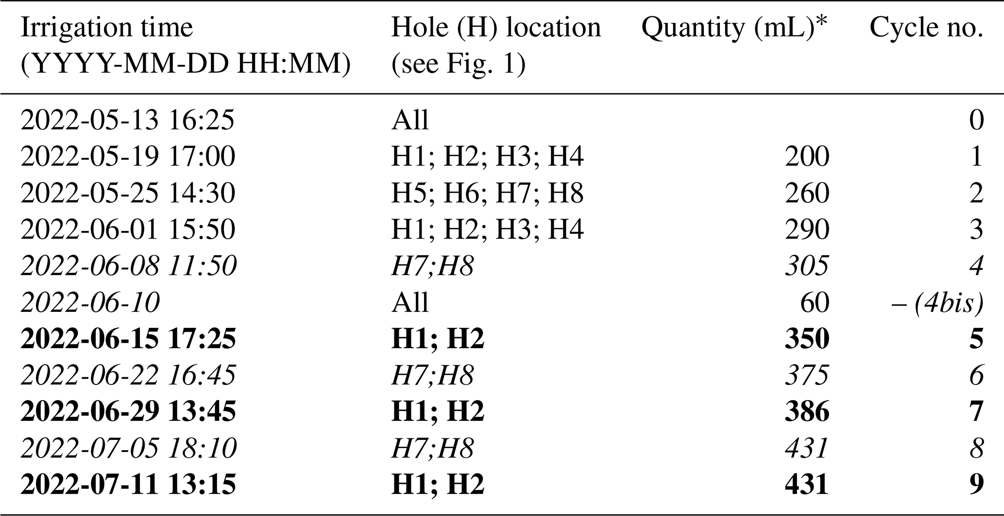
∗ Quantity in total distributed over all the holes.
2.2 Electrical resistivity tomography
Electrical resistivity tomography consists in reconstructing the subsoil ER using an array of electrodes (Binley and Slater, 2020). In this study, a total of 72 stainless steel electrodes were used; 64 electrodes formed a grid, 5 cm spaced, covering the screening face of the rhizotron, and an additional line of eight electrodes was posed at the top surface. Electrodes are needles 4 mm in diameter and 80 mm in length, but only their tip is in contact with the soil. ERT involves the measurement of transfer resistances following a sequence describing a combination of varying injections (AB) and potential (MN) pairs of the electrodes. We used a custom sequence composed of 4968 quadrupoles including the reciprocals (e.g. Parsekian et al., 2017), and the measurement were conducted using a Syscal Pro (Iris Instrument) resistivity meter. The sequence was optimised over the 10 physical channels of the instrument in order to reduce the acquisition time to approximately 30 min. The data acquisition parameters were constant along the monitoring, with a minimum required Vp of 50 mV, a maximum injection voltage VAB of 50 V, and a number of three to six stacks with the on time fixed to 250 ms each.
2.3 Electrical current imaging
The electrical current imaging (or mise-à-la-masse) method was logistically similar to ERT. The sequence nevertheless varies, as the pairs of injection electrodes were kept constant with the positive pole (+I) electrode located on the stem and the return (−I) electrode located in the bottom right of the rhizotron. The potential electrode pairs (MN) vary according to a custom sequence. For the stem current stimulation, we inserted a small stainless steel needle (2 cm, 1 mm diameter) into the plant stem at 5 cm from the grafted point. The needle was inserted all the way to the centre of the stem (Fig. 1). Before each measurement, we added a few drops of water to the stem needle in order to reduce the stem contact resistance (to values between 41 and 66 kΩ). The current was guided to the root system via the stem and then released into the soil.
As the effect of the stem contact resistance affects the measured voltage, a control soil injection was systematically made. In that case, the current was injected into the soil close to the plant (Fig. 1). A qualitative comparison between the control soil injection and the stem injection plant could be made to discriminate the effect of roots. Furthermore, soil control injection served as a visual calibration for the inversion of the current source knowing that the injection is punctual and occurs at a known position.
2.4 Weight monitoring for the estimation of transpiration
In order to track the weight changes due to the transpiration of the plant, the rhizotron was equipped with a single point load cell (PC60-30KG-C3, Flintec), mounted between two plates in plexiglass supporting the rhizotron (Fig. 1). The data were logged with a sampling rate of 5 min using the weight indicator DAD-141.1. The total weight of the rhizotron is about 20 kg, and the expected resolution according to the sensor data sheet is 0.1 g. The variation due to temperature was monitored, on average, in May at 22 ∘C and in July at 25 ∘C. To avoid sharp signal perturbation, the logger was paused during the irrigation and the acquisition of geophysical data.
2.5 Leaf gas exchange observations
In order to monitor the physiological response of the plant during the course of the experiment, stomatal conductance to water (gsw []) measurements were performed on vine leaves with an open flow-through differential porometer (LI-600, LI-COR Inc., Lincoln, Nebraska, USA). The stomatal conductance is a measure of the density, size, and degree of opening of the stomata; therefore it can be used as an indicator of plant water status (Gimenez et al., 2005). The measurements were carried out on 26 leaves in the morning hours (at 10:00), once (on 8 June 2022) just before irrigation (severe water stress), and once (on 16 June 2022) 1 d after irrigation (mild to low water stress). For the tracking of the plant development, the length (L) and the width (W) of every leaf were measured every 2 weeks from the beginning of the growing period until the end of the experiment. From these data the total leaf area (LA) was estimated according to three models: LA1=0.587 (L×W) (Tsialtas et al., 2008); (L×W) (Elsner and Jubb, 1988); (Elsner and Jubb, 1988).
2.6 Data processing
2.6.1 Analysis of ERT data
The ERT acquisition sequence was initially tested on the rhizotron filled with water of known conductivity, and it offered good coverage on most of the rhizotron surface with a slight decrease on the sides. The soil electrode contact resistances varied over the course of the experiment between 5 and 20 kΩ. Data were filtered on the basis of the percentage of variations between direct and reciprocal measurements. We chose to eliminate the data with reciprocal relative errors larger than 5 %, for all the time steps. The number of rejected data varies from 9 % to 39 % of the total (see Table A1) with a median of 11 %. Transfer resistances were inverted using the open-source code ResIPy (Blanchy et al., 2020) based on the Fortran R3t code (Binley, 2015). The inversion mesh is an unstructured grid composed of tetrahedra, created using Gmsh (Geuzaine and Remacle, 2009). Two distinct strategies can be used: (1) individual inversion, which consists of building a model of resistivity at a given time, and (2) time-lapse inversion (difference inversion) where the difference in resistivity is inverted between a given survey and a background survey (in this case, the background survey is the previous one). In this study, we used the first approach, which allowed the filtering of systematic noise and highlights variations (as a percentage of differences) between two times.
2.6.2 Analysis of current density
The mathematical formulation for the inversion of the current source density (CSD) has been developed in previous studies. It consists in searching for a linear combination of Ohm's law, for a series of current punctual sources (also called virtual sources) minimising the misfit between simulated and observed data. The algorithm was initially tested on the rhizotron filled with water of known electrical conductivity and a single isolated cable (see the procedure from Peruzzo et al., 2020). It is important to note that the CSD inversion relies on the knowledge of the medium conductivity (as in the Poisson's equation, the current is modulated by the electrical conductivity). Thus, we used the inverted ER values as the resistivity distribution for the forward modelling in the current density inversion. As for ERT, choices must be made on how data and models are weighted and regularised during the inversion. In this study, we run unconstrained (no prior information) inversions for all the time steps with a regularisation (smoothing using the first derivative). The numerical routine includes a “pareto” functionality, wherein regularisation and model-to-measurement fit are traded off to estimate the optimum regularisation weight wr. The code used for this inversion is available at https://github.com/Peruz/icsd (last access: 21 November 2023).
2.6.3 Calibration of petrophysical relationships
In order to estimate the soil water content in the rhizotron during the experiment, we needed to adopt a suitable constitutive model, starting from the available ER measurements.
Archie's (1942) law (Eq. 1) is a widely used empirical relationship that relates the ER (ρ) of a bulk material to its porosity (Φ), the contained fluid (water) electrical resistivity (ρfl), and the fluid saturation (S). Archie's parameters a, m, and n are empirically derived and generally named as follows: a is the tortuosity factor, m is the cementation exponent, and n is the saturation exponent.
We calibrated these parameters experimentally, as is usually done, by collecting water saturation ER values over different soil samples. The sample holder (a cylinder of 150 mm inner height and 41 mm inner diameter) allows for a four-point measurement of the ER converted to apparent ER using the appropriate geometrical factor. The adopted water electrical conductivity is known and fixed (594 µS cm−1 at ∼25 ∘C). The rhizotron soil mixture porosity was assumed to be equal to 0.55. The sample was initially saturated to field capacity and progressively desaturated. The field capacity was estimated by gravimetric method approximately at 40 % of volumetric water content (m3 m−3). In total, six measurements were collected at respectively 40 %, 33.6 %, 29.7 %, 28.2 %, 25.2 %, and 22.4 % of volumetric water content (m3 m−3). The obtained data are fitted with a least square optimisation (using the Scipy library by Virtanen et al., 2020). Here we assume a equal to 1 (consistent with the theoretical value), while the exponents m and n are bounded during the optimisation process to respectively [1.3–2.5] and [1–3]. With a coefficient of determination R2 of 0.97 (figure not shown), we obtained values of 1.9 and 1.2 respectively for m and n.
3.1 Physiological response
Photographs of the plant at the beginning and at the end of the experiment show the increment of leaf area extension of the aerial part. The weekly measurements show a linear trend with time of the estimated total LA (cm2) regardless of which LA the model used (Fig. 2). At the end of the experiment water stress symptoms were visible on some leaves.
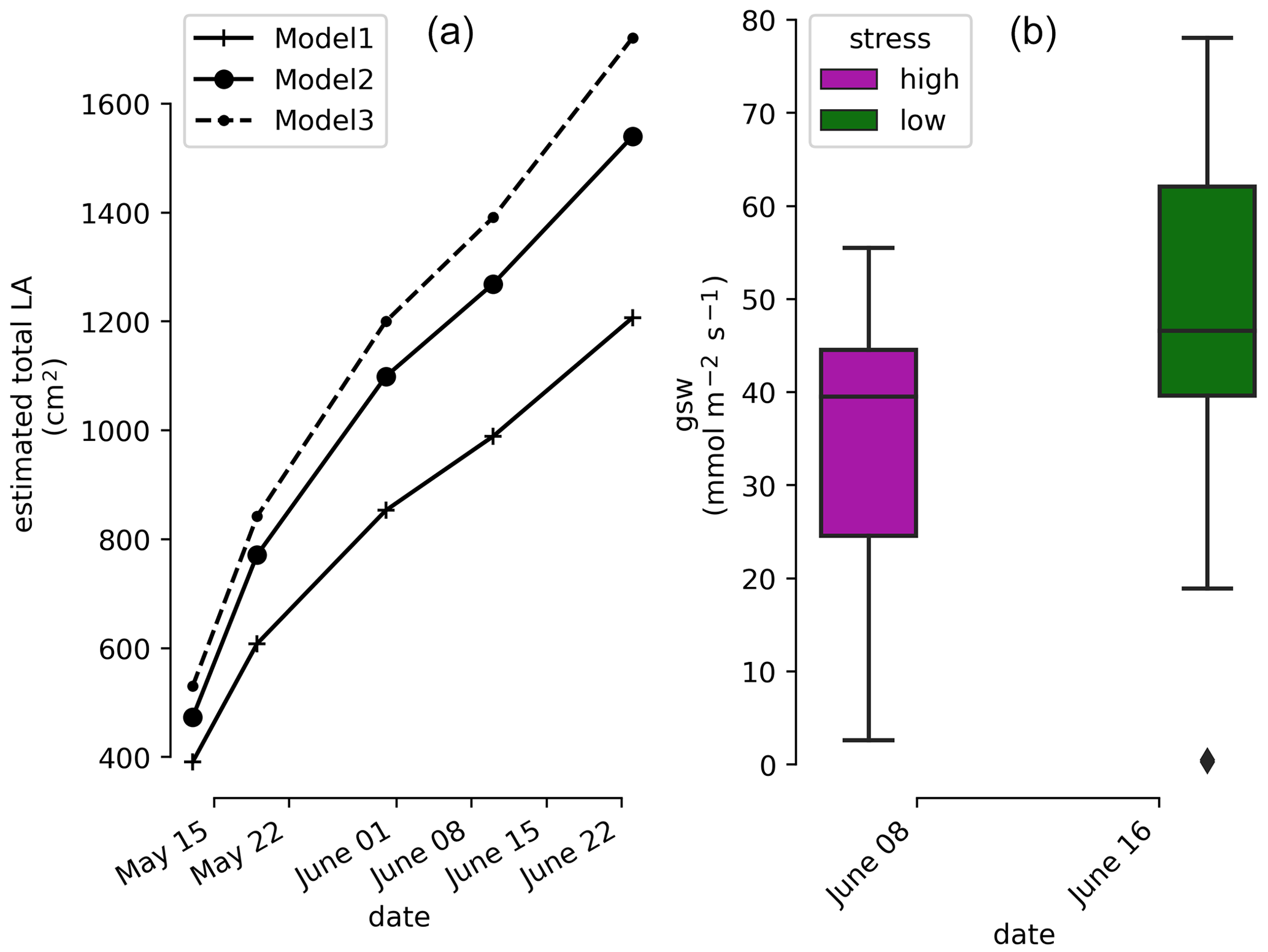
Figure 2(a) Time evolution of the estimated total leaf surface area (LA) for three different model estimators. (b) Leaf stomatal conductance (high- and low-stress distributions are significantly different with a t test ).
As for the root system, the depth variations could not be precisely assessed during the course of the experiment. We observed that (i) roots reached the bottom part of the rhizotron; (ii) roots spread all over the rhizotron with a network of primary, secondary, and root hairs without any given architecture (some roots grew vertically, others in diagonals); (iii) the roots kept a white appearance with apparently no lignification even for the largest roots (≧3 mm).
The measurements shown come from the 26 leaves (cf. Sect. 2.5) and indicate that the plant is under high water stress at the end of the irrigation cycle (1 week after the last partial irrigation, on 8 June 2022) and under lower water stress 1 d after irrigation (on 16 June 2022). The mean, min, and max values of the stomatal conductance (gsw) values are 37.8, 23.3, and 55.5 before irrigation respectively and 50.6, 18.9, and 78.1 after irrigation respectively. The result of the t test shows that their mean values are significantly different ().
3.2 Transpiration rate
No pre-processing of the raw data is needed for their interpretation. Figure 3 shows that, on average, during a PRD cycle (about 1 week), 0.5 kg of water transpired. Also, the weight data show that the total weight is decreasing from one cycle to the next, as expected, due to the PRD protocol. Although the total water content is decreasing, the transpiration rate (slope of the weight variations) remains constant for each cycle. At the very end of the experiment from 9 July, an inflexion point is observed and the weight stops decreasing. Zooming on a shorter time window, the variation in the raw data weight clearly shows day–night patterns triggered by the hours when the light is switched on/off. On average, the water lost during the day is nearly 20 times more than during the night (0.09 kg vs. 0.005 kg, day vs. night, respectively). Note that there is no distinction between the hours of the day (due to artificial lighting).
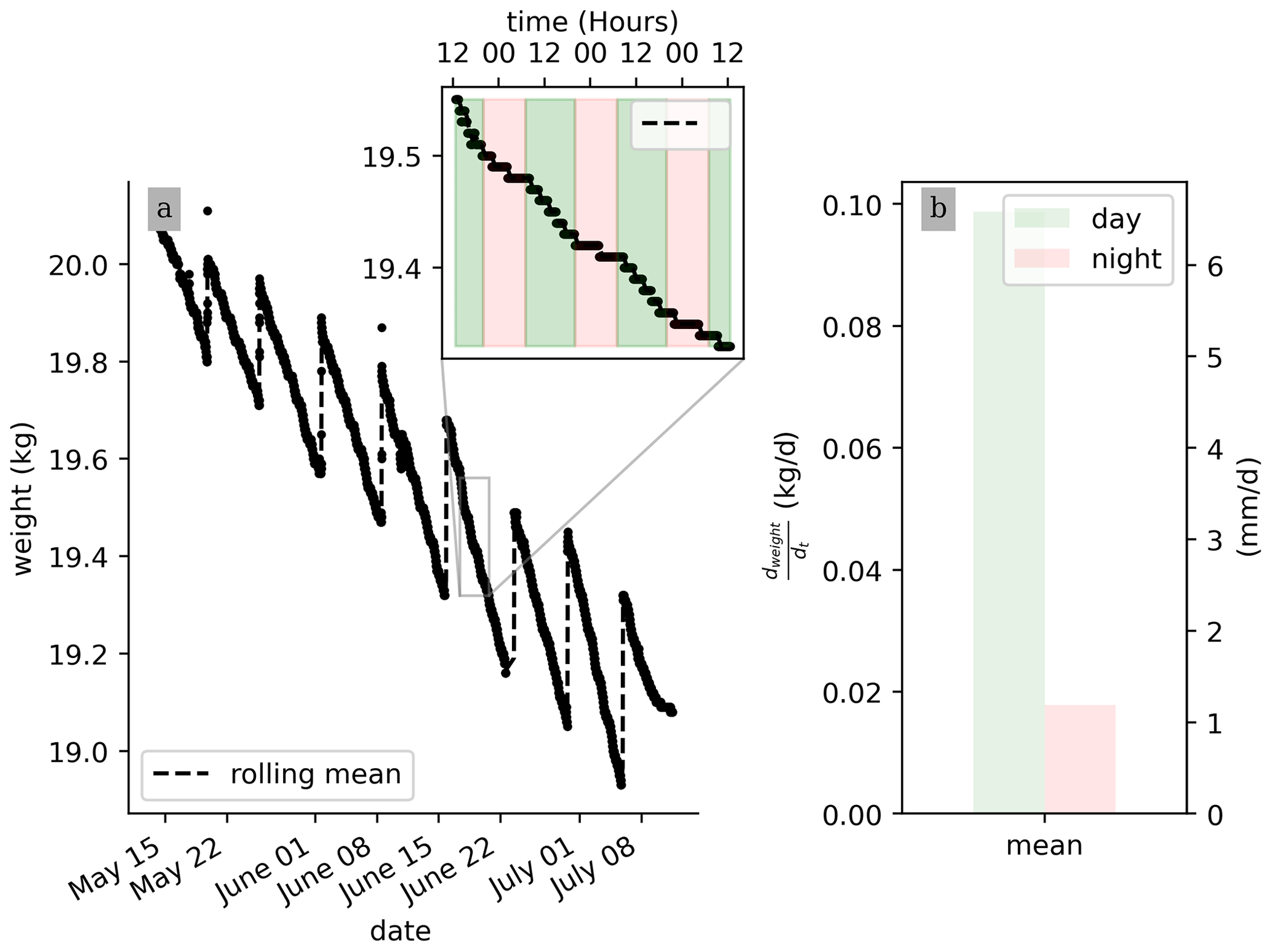
Figure 3Raw-scale data collected over the course of the experiment (a) and a zoom on the week of 20 to 25 June, where day and night periods are respectively highlighted by the green and pink shaded areas. (b) Calculated daily mean transpiration () during the day (green) and night (pink) periods.
3.3 Time-lapse ERT
In general, the ERT data quality is very good with a small percentage of total measurements exceeding a reciprocal noise level of 5 % (see Figs. A1–A11) and with each inversion resolved within two or three iterations. Figure 4 shows the trend for the PRD cycles (from cycles 0 to 9) for the mean average electrical conductivity (in mS m−1) for both the wet and dry sides of the rhizotron, taken as an average of each half of the ERT inversion mesh elements. When PRD is applied over only two holes (from cycle 4) the irrigated side shows a clear increase in electrical conductivity. To a much lower degree, the dry side is also affected by the water input, likely due to water redistribution during drainage. When available, the temporal dynamics between two irrigations show that the conductivity is decreasing rapidly on the irrigated side during the 2 first consecutive days and more slowly afterwards (cycles 5/6 and 7/8 respectively; Fig. 4c and d). As some water infiltrates also on the dry side, we also observe an increase in conductivity in it. At the end of each cycle (the cycle length is about 7 d), the rhizotron returns to the equilibrium condition, with a more homogeneous and stable average conductivity equal to 30 mS m−1 (mean of the dry and wet sides). This is generally true for all times, except at the end of the experiment, cycles 7 and 8, when the two sides are in different conditions.
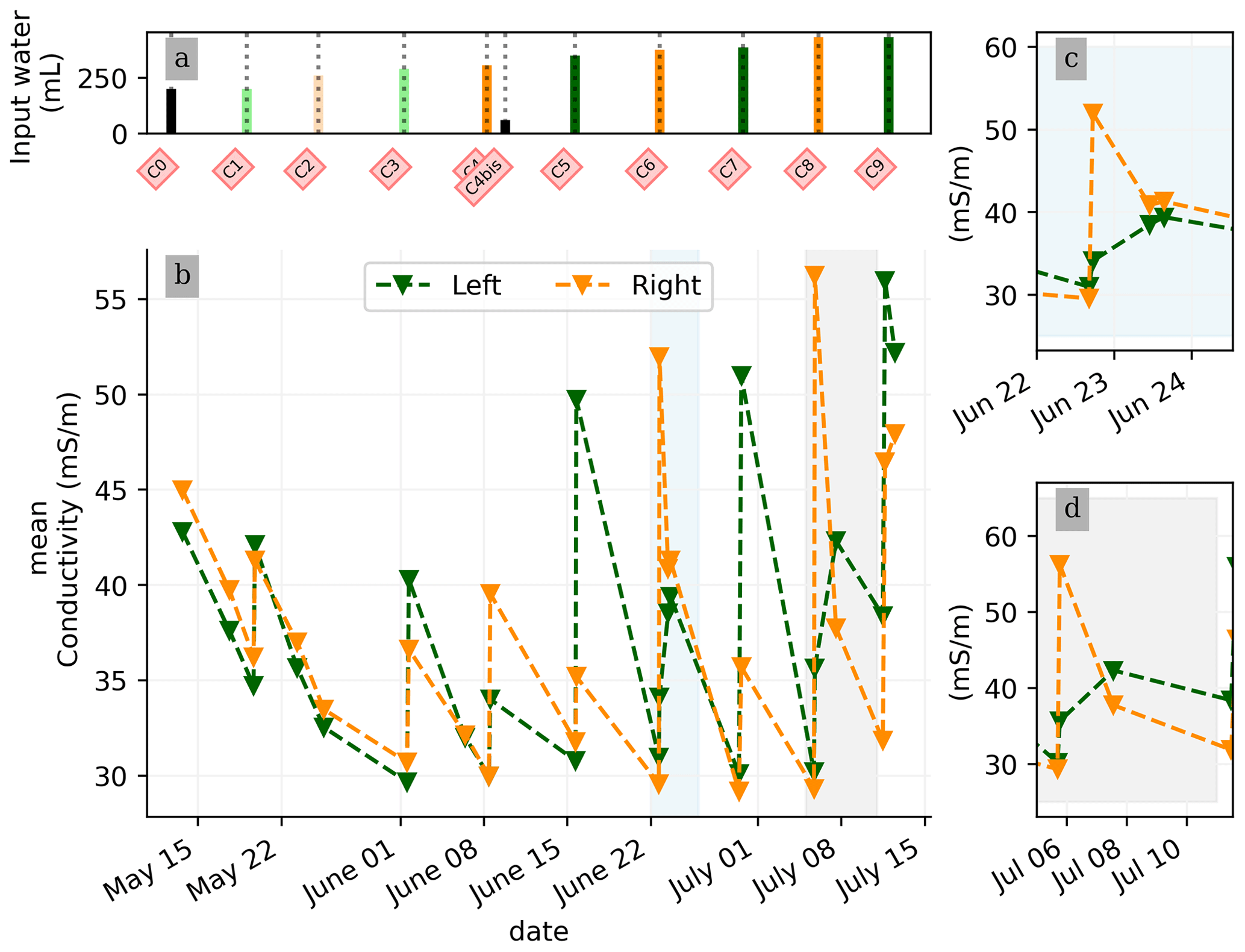
Figure 4(a) Evolution of the quantity (in mL) of water input, spatially distributed with alternating between left (green) and right (orange) before and during the PRD irrigation. (b) Evolution of the mean conductivity (mS m−1) average on each side; markers show the acquisition time. Panels (c) and (d) are inset zooms showing changes before and just after the irrigation event.
We selected a time window between 29 June and 5 July showing the spatial variations in the ER before and after an irrigation event (Fig. 5). The application of background constraint inversion, as illustrated in Fig. 5b and c, leads to an interpretation suggesting that the blue regions correspond to areas where the soil is wet, whereas the red regions correspond to areas where the soil is drying. Before the irrigation, the top and left-most and right-most boundaries of the rhizotron exhibit higher ER (50 Ω m) than the central part (25 Ω m). One hour afterwards (+1H) the ER of the left irrigated side had dropped by 20 % (estimated from the averaged values extending from the middle of the rhizotron to the left boundary).
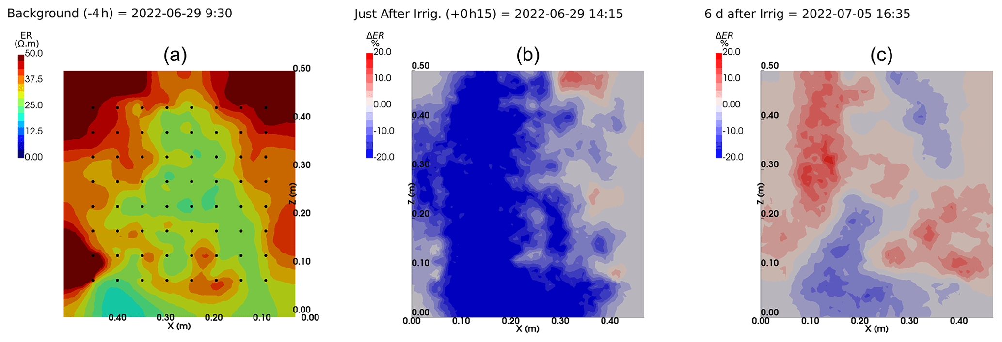
Figure 5Spatial distribution of the resistivity (in Ω m) and changes (in %) in ER obtained by a time-lapse inversion between cycle 6 and 7 following partial left irrigation of the rhizotron. Time steps correspond to measurements before (a) and 15 min (b) and 6 d (c) after irrigation started.
All time-lapse inversions before/after irrigation are shown in Appendix A, including before the PRD. They all show that a decrease in ER is associated with irrigation patterns, while an increase in ER has more complex spatio-temporal dynamics, not systematically associated with irrigation patterns. Positive alterations in resistivity observed immediately after the irrigation event may potentially be artefacts stemming from a strong gradient in resistivity induced by the irrigation. Changes in ER after 6 d (day + 6) show that RWU effects are not limited to the irrigated part since the increase in resistivity was also observed on the dry part. We noticed from a visual inspection of the rhizotron that a water table forms at 0.4 m where the soil is saturated. This saturated zone level is not affected by the irrigation as no increase after irrigation and no decrease by the end of the irrigation cycles are visible. We assume that most of the water fluxes were connected to the unsaturated part.
3.4 Time-lapse ECI
Figure 6 shows the trend of the horizontal location (x coordinate) of the centre of the mass of current density during the PRD cycles (from 0 to 9), after the alternative wetting events on the left and right sides of the rhizotron. Considering the modulation of current by soil electrical resistivity (ER), any bias in ER could introduce errors in forward current source imaging and, consequently, affect the positioning of the current source. The centre of mass of the soil CSD is not shown as it is always pinpointed to the location of the injection electrode whatever the irrigation pattern, as expected (Fig. 7a–c). This result confirms the quality of the estimated ER background values used for the ECI forward model. For the stem injection, the centre of mass of the current source density is distributed equally from left to right except for cycle 4 when most of the current is located on the left (see Figs. B1–B4). Conversely to ER variations, the irrigation pattern does not significantly affect the current density distribution. The same applies to the temporal dynamics between two irrigations where the current density centre of mass is stable and distributed equally on both sides, as shown in Fig. 7. All the time-lapse inversion results of current density for the soil and the stem injection are shown in Appendix B.
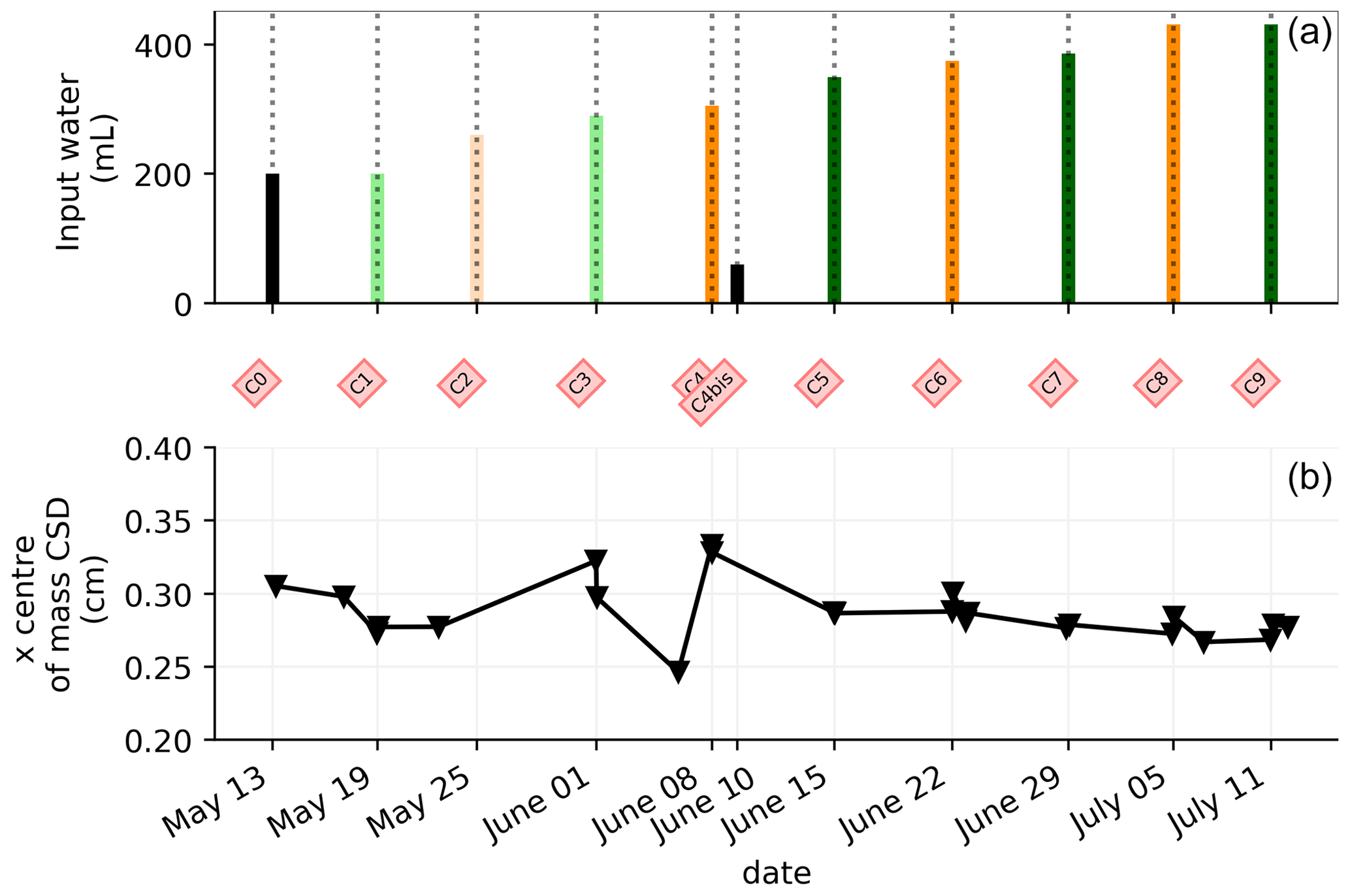
Figure 6(a) Evolution of the quantity (in mL) of water input spatially distributed alternatively between left (green) and right (orange) during the PRD irrigation. (b) Evolution of the centre of mass (in the x direction) of the current density, while cross markers show the acquisition times. Cycle 6 to 7 windows were selected for the MALM time-lapse spatial analysis (Fig. 7).
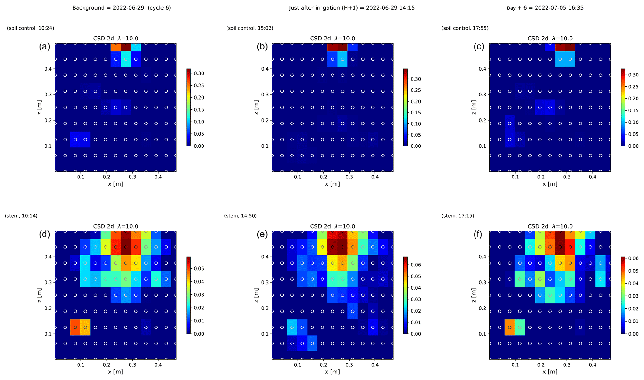
Figure 7Spatial distribution of the CSD between cycles 6 and 7 following partial (right) irrigation of the rhizotron for the soil control injection (a–c) and the stem injection (d–f). The larger spread of current sources in the stem injection (d–f) compared to soil control injection (a–c), demonstrates that the root system plays a key role in the distribution of the current source in the soil. Time steps correspond to measurement before (a, d) irrigation, 1 h after irrigation (b, e), and after 6 d (c, f). The regularisation parameter wr is fixed to 10 for both cases (see Sect. 2.6.2 for the choice of wr).
3.5 Correlations between soil parameters and estimated transpiration rates
This section aims at drawing correlations between the soil parameters (ER, SWC, and CSD) and the transpiration estimated from the rhizotron weight data. We do not account for the weight variations due to the plant and root growth material (as this can be considered negligible relative to water dynamics). For each node of the mesh, ER values are translated to SWC using Archie's law with the calibrated parameters m and n (see Sect. 2.6.3). Averaging is performed on the mesh nodes falling within each side, with the middle point being defined as half of the rhizotron width, equivalent to 0.25 m. To simplify, we assume that both porosity and fluid water conductivity are homogeneous in space and time (i.e no mixing between the tap water used for cycle 3 and the nutrient solution for all the other times). The maximum SWC observed after irrigation is about 0.42 m3 m−3 (figure not shown). The minimum SWC of about 0.25 m3 m−3 is repeatedly observed (see Fig. C1) just before each irrigation, meaning that the driest times are below field capacity conditions (estimated at 0.4 m3 m−3). By examining the fluctuations in weight, one can calculate the corresponding changes in spatially averaged water content. Figure 8a illustrates a linear trend (R2=0.83 and ) between the inferred water content variations from the scale and those obtained from ERT (after Archie transformation). The most significant positive changes in averaged water content are attributable to the triggered irrigation, leading to a ΔΘ (change in water content) of −0.1. Conversely, negative changes primarily result from transpiration, with a maximum value located at +0.1.
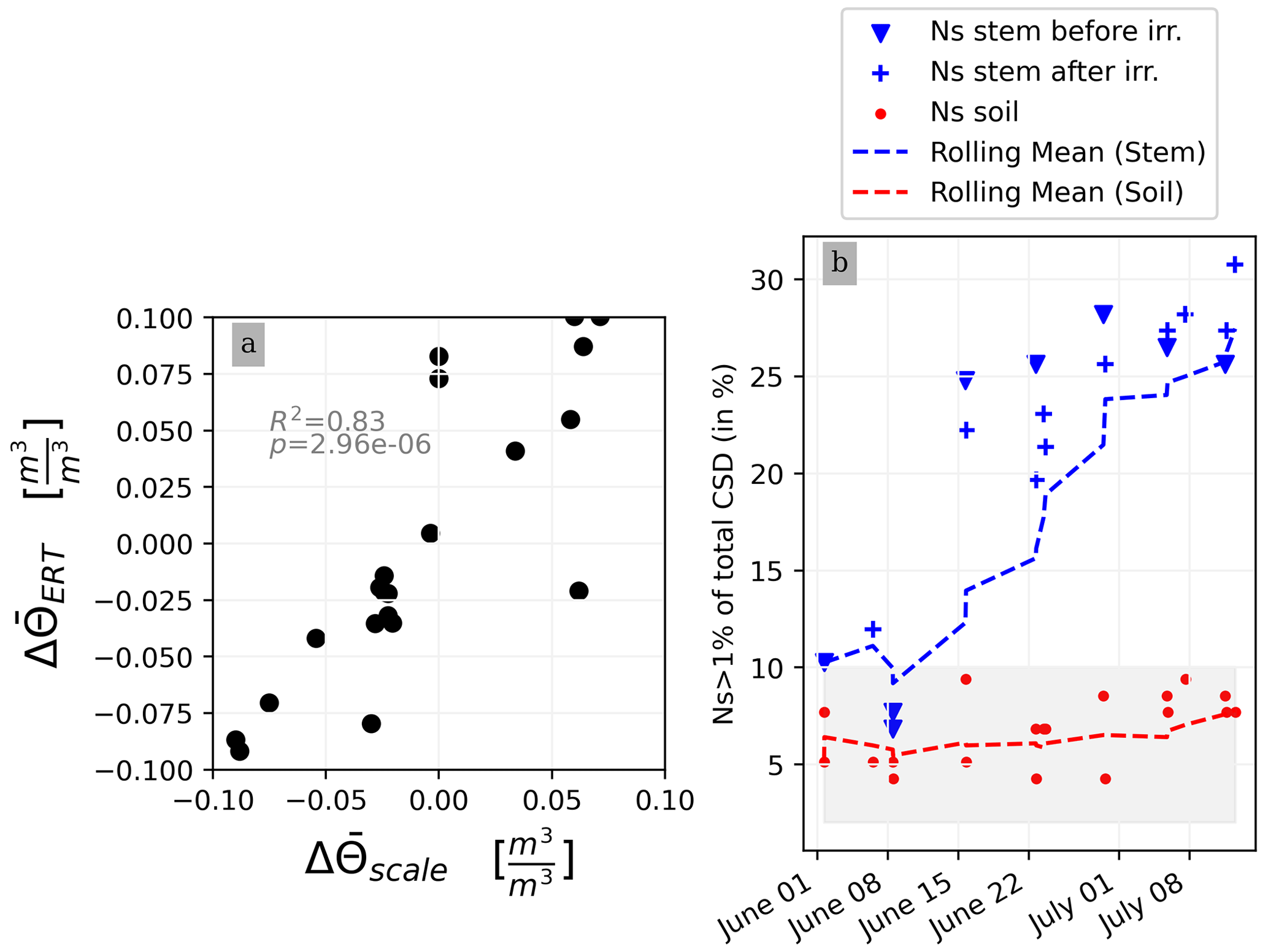
Figure 8(a) Changes in water content calculated from weight changes related to the changes in water content calculated from the ERT measurements. (b) Relationship between the number of the current sources (Ns) carrying at least 1 % of the total density (A m−2) with respect to the time of the experiment. CSD results are obtained after inversion with a regularisation parameter wr of 10. Cases of the stem before cycle 3 (grey) and after cycle 3 (black) and the soil (blue) injections. All cycles are considered.
Figure 8b shows the relationship between the variation in the percentage of the current sources carrying at least 1 % of the total density (Ns1) used as an estimator for current density dispersion with respect to the date time of the experiment. For the soil injection (red dots), Ns1 is relatively constant between 5 % to 10 % of the total number of possible injection nodes (grey area). For the stem injections, Ns1 increases over the course of the experiment. From 1 June to 8 July, Ns1 triples. The is no distinction between Ns1 measured before (triangles) and after (crosses) irrigation.
4.1 Validity of ERT and ECI in demonstrating the effects of the alternating irrigation scheme
Our first assumption was that the variations in ER (or in SWC inferred from the ER) are relevant as a proxy for root activity. Their validity has been checked against direct observation using the variations in weights measured from the scale data used as an indicator of plant transpiration. On average, in our experiment, the plant maintained high rates of transpiration to about 6 mm d−1 for each cycle except for the last cycle (number 9) where a decline was observed (Fig. 3). This range is in line with another rhizotron experiment where narrow-leaf lupin plants were grown: Garrigues et al. (2006) measured a mean rate of 3 mm d−1. It is commonly found in the scientific literature that changes in ER are associated with root activity (e.g. Michot et al., 2003; Garré et al., 2011; Cassiani et al., 2015; Whalley et al., 2017). Here we had further confirmation of this, with a significant correlation between ER changes and gravimetric soil moisture changes (derived from the load cell) (Fig. 8). The leaf stomatal conductance and visual observation of plant above- and below-ground material growth were additional ancillary data to interpret the general state of the plant. Our observation is in line with the literature; i.e. in general, low soil water content (SWC) can lead to drought stress in plants, which can result in decreased leaf stomatal conductance and less transpiration and vice versa.
A second assumption was that, when applying the alternative irrigation scheme, only one part of the root system would be active and the current injected into the stem would only spread to the side where the root system is irrigated. This assumption was not directly supported by the observations. Figures 6 and 7 show that the influence of the irrigation pattern was negligible on the spatial distribution of the inverted CSD and that the current distribution was not correlated with ER variations. It is true that active roots have higher hydraulic conductivity, but on the other hand, increased membrane permeability may encourage current leakage into the soil. We nevertheless noticed that the CSD spatial distribution, while the rhizotron is irrigated at its full length (cycles 0 to 3), was significantly different from the side irrigation cycles (Fig. B4). Indeed, homogeneous irrigation without applying stress to the plant results in a very shallow current leakage. Our observations potentially suggest that under conditions where soil electrical conductances are high near the soil–root interface – and even if there is good electrical contact between soil and roots – the distribution of current source density might not be directly related to water uptake distributions. Further research is needed to confirm this potential relationship.
4.2 Effect of soil water content and transpiration demand
Soil water content can affect the distribution of the current leakage by influencing the minimum resistance pathways, i.e. whether roots and/or soil provide the minimum resistance to the current flow. Literature reports that the electrical capacitance method better estimates crop root traits under dry conditions (Gu et al., 2021). In order to make a comparison with capacitance studies, we assumed that if the current distribution remains unchanged (i.e. leaking into the same areas), there must be minimal changes in the electrical capacitance. In this study, supposing no impact of the initial model, Fig. 8 shows that there is no apparent effect of the soil water content on the current density distribution. Note that the soil water content estimated is the bulk contribution of roots and soil, as only one pedophysical relationship was used, while recent studies tend to show that mixed soil–root pedophysical relationships are preferable (e.g. Rao et al., 2018). Moreover, considering small-scale variations around individual root segments in terms of water content and soil hydraulic properties becomes crucial for a comprehensive understanding of the system. This is clearly limiting our ability to interpret the independent contribution of the soil and the roots, yet this does not limit our ability to identify zones where water availability leads to root water uptake.
Based on Figs. 2 and 8b, the association between water stress and leaf development, along with transpiration demand, is expected to be more prominent (and increasing during the course of the experiment rather than the specific time points before and after irrigation). Indeed the fluctuations in water content during various cycles, with or without stress, exhibited remarkable similarity. Both stressed and non-stressed cycles experienced a drop in water content to similarly low levels. Consequently, water content does not appear to account for the variability in water stress. Instead, it is the increased transpiration demand over time that seems to play a more significant role in driving the observed changes. At high transpiration demand, stress may occur at higher soil water contents because the soil becomes limiting for the root water uptake. The changes in water potential and water content in the vicinity of the soil–root interface can potentially impact the electrical conductivity of the immediate soil surrounding the roots. Consequently, as the experiment progressed, lower electrical conductances in the soil around the roots potentially led to a restriction in the flow of current between the root system and the soil. This, in turn, may have resulted in a more uniform distribution of the electrical current source along the entire length of the root system.
4.3 Possible mitigation of the PRD effect
In general, a PRD irrigation experiment must comply with two criteria: (1) a minimum soil water content to trigger a physiological response and (2) a distinction between a wet and a dry side (Stoll, 2000; Stoll et al., 2000). In our experiment, the first criterion was met but not the second. This provides an interesting piece of evidence, leading to the following considerations:
-
According to McAdam et al. (2016) and Collins et al. (2009), ABA is triggered even by mild soil stress values. Consequently, plants adapt the hydraulic conductivity of their roots as well as that of the soil in their vicinity through exudates (Carminati and Javaux, 2020). Results from previous irrigation experiments using PRD or DI have shown that changes in stomatal conductance and shoot growth are some of the major components affected (Düring et al., 1996). In our experiment, the shoot growth was fitted with the conventional leaf area and growth models, except at the end of the experiment when signs of water stress were visible on some leaves. The magnitude of the shoot growth is correlated with the number of roots. Drought may cause more inhibition of shoot growth than of root growth (Sharp and Davies, 1989). Although the root system was already well developed, it is not possible to exclude its development as a factor influencing the CSD distribution.
-
The spatio-temporal analysis of the ER showed that the water changes were not limited to root effects. Water redistribution from dry to wet in the soil and from shoot to dry roots (Smart et al., 2005; Lovisolo et al., 2016) may have occurred (Figs. A1–A11). Additionally, although it is not visible from the screening face, capillary rise may have taken place due to the presence of a saturated zone at the bottom of the rhizotron. Due to the fact that water drained on both sides, RWU was not only vertically distributed but also horizontally. The range of water content varied significantly with a minimum SWC of about 0.25 m3 m−3, repeatedly observed just before each irrigation meaning that the driest times are below field capacity conditions (estimated at 0.4 m3 m−3). Drying half of the root system resulted in a reduction in the stomatal conductance (based on the mean of the distribution) of the order 5 after a 1-week cycle. Given the stress applied, the ER changes highlighted that roots played a major role in the vine plant survival and evidenced strategies of adaptation. Indeed, the plant was able to adjust its water uptake and redistribution zones depending on the water availability, from all places, not only from the alternate irrigated areas.
-
Finally, in order to know if the PRD conditions are met it would have been important not to neglect the different states of root growth and root renewal (because of renewal and decay) with respect to the geophysical data. Nevertheless, this would have required opening and scanning the rhizotron with conventional methods. Finally, we did not make a distinction between the hours of the day although the changes observed for the irrigation are rapid, usually at the hourly scale, and could be similar for RWU.
4.4 Performance of the acquisition protocol and the processing
We discuss here the quality of the recovered current density models by evaluating the performance of the protocol and the processing. First, it is important to note that although the ERT data quality was good (very few reciprocals were rejected; see Table A1), the inverted model was not perfect and this ultimately has an impact also on the ECI forward model. The algorithm has undergone testing in a rhizotron experiment and has demonstrated the ability to differentiate punctual sources, even when their current contribution is as low as 5 % of the total current (Peruzzo et al., 2020). The CSD resolution, of course, matches the electrode interspace (in this case 5 cm), and the smoothness constraint does not impact the simulation of point source reconstruction. We adopted an inversion without any prior information to recover the current density. Only model smoothing was applied by weighting the model data by an optimal factor of 10 inferred from an L-curve analysis. Similar to the ERT inversion, the CSD problem is also ill-posed. In this case, the four-electrode setup ensures that the current will flow through the plant after injection, regardless of the contact resistance. However, the accuracy of the measured data may be impacted by contact resistance, as errors in the measured resistance will negatively affect the quality of ERT and CSD inversions. The impact is more pronounced on CSD, as it is dependent on ERT. Lastly, because the box is relatively small and no current-flow boundary conditions (Neumann) are imposed, we may expect an effect due to the position of the return electrode where the current is attracted due to the strongest gradient nearby (Mary et al., 2019a).
4.5 Outlook
In order to strictly correlate PRD effects with geophysical measurements, one should consider a physical barrier to separate the two sides of the rhizotron to a split-root configuration. Another option is to increase the lateral size to prevent redistribution or to use a very percolating material such as glass beads, gravels, or coarse sands. This should be carefully considered, as the rhizotron must also be an environment where plant growth is possible under “natural” conditions, and for this some water retention capacity is needed for the soil. A larger drainage capacity would simplify the interpretation as no water redistribution from one side to the other can occur. Although considering a barrier is technically possible, it would require a more complex inversion scheme of the ERT and ECI considering that no electrical current can flow from side to side. One could also consider increasing the measurement frequency to catch processes at an hourly scale and comparing day–night measurements, particularly those associated with water redistribution from the stem back to the roots at night, when transpiration is reduced, and its effect on the water status of the roots. As we have seen that most of the water changes occurred in the day consecutive to the irrigation, catching rapid changes in ER would help draw a conclusion on how much ECI is connected to the active root zone. Finally, in order to draw robust statistical conclusions, the experiments should be replicated for multiple plant samples.
The study aimed to understand the current path in the root system and active root zones using geoelectrical imaging, considering soil water content and irrigation regimes. Electrical resistivity tomography (ERT) is sensitive to both irrigation and RWU processes. The ECI model uses a physical approach to measure current density after stem stimulation. The CSD was very different from the control soil injection to the stem injection but nevertheless did not correlate with PRD cycles as originally expected. We demonstrate that under mild stress conditions, it is practically impossible to spatially distinguish the PRD effects using the ECI. We only evidenced that the current source density distribution varied during the course of the experiment considering evaporative demand but without any significant relationship to the soil water content changes. A few aspects of the experiment would gain from being more closely studied such as the water redistribution that possibly also affects current distribution. In the future, we expect to improve our understanding by coupling the geophysical experiment with an unsaturated soil–plant–atmosphere model.
As we selected only one cycle in the paper, we report here further details about the time-lapse ERT inversion results for all the cycles. The inversion procedure is equivalent to the one described in Sect. 2.6.1 of the paper (“Analysis of the ERT data”). All time-lapse inversion models are plotted with a unique scale ranging from −20 % to 20 % of changes.
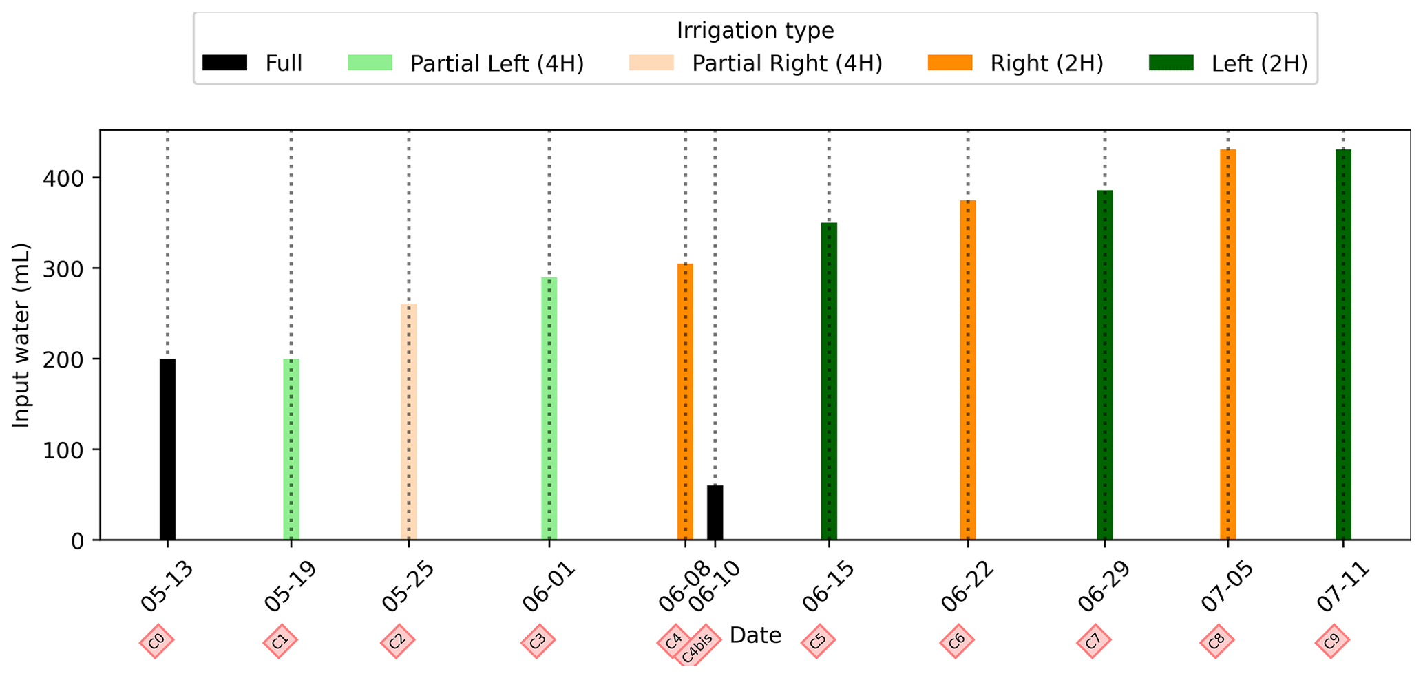
Figure A1Evolution of the quantity (in mL) of water input spatially distributed with an alternation between left (green) and right (orange) during the PRD irrigation. The black bars are applicable for full-width irrigation (over all the holes; see Fig. 1), light green and orange bars are applicable for irrigation over the four sides of holes, and dark green/orange is applicable for two-hole irrigation.
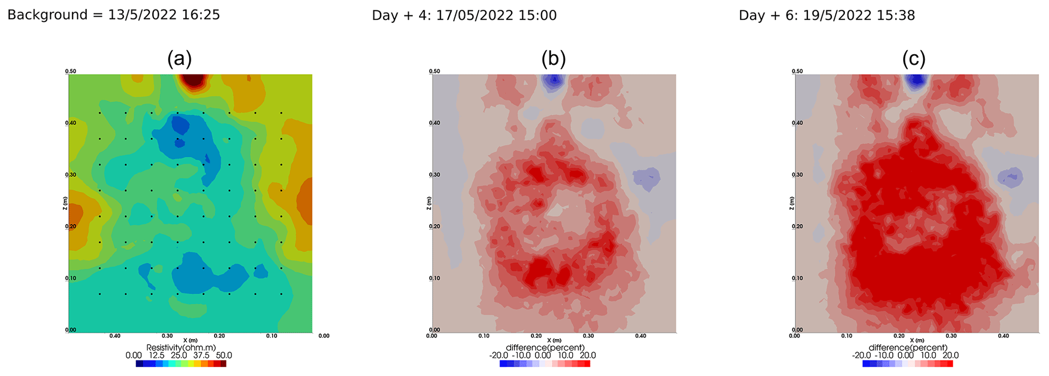
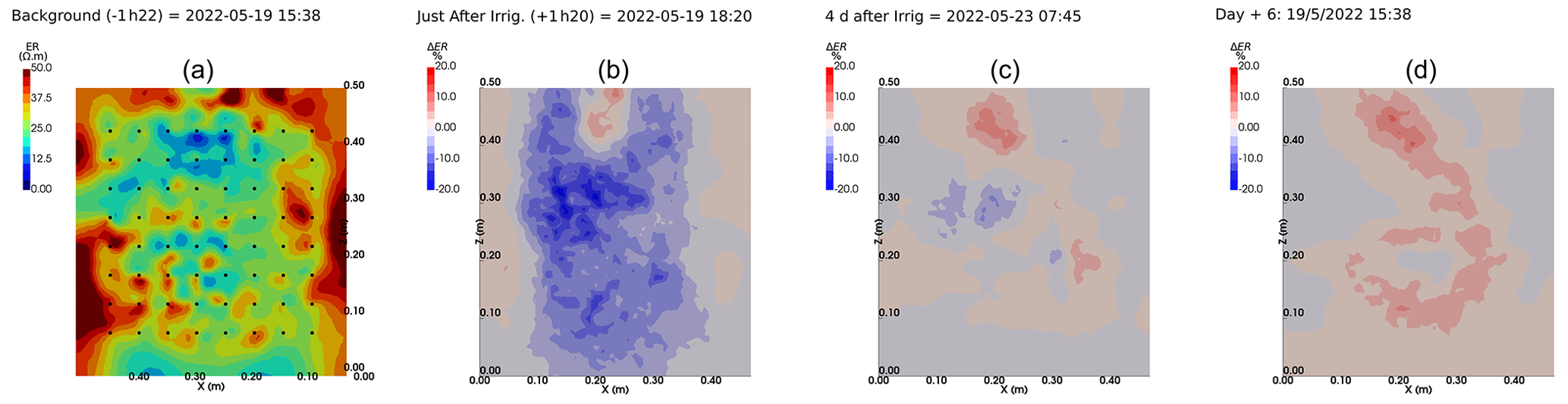
Figure A3Cycle 0 to 1 (partial irrigation: 19 May 2022, 17:00–17:30, 200 mL, through the first four upper holes (left side); no outflow through the outlet point).
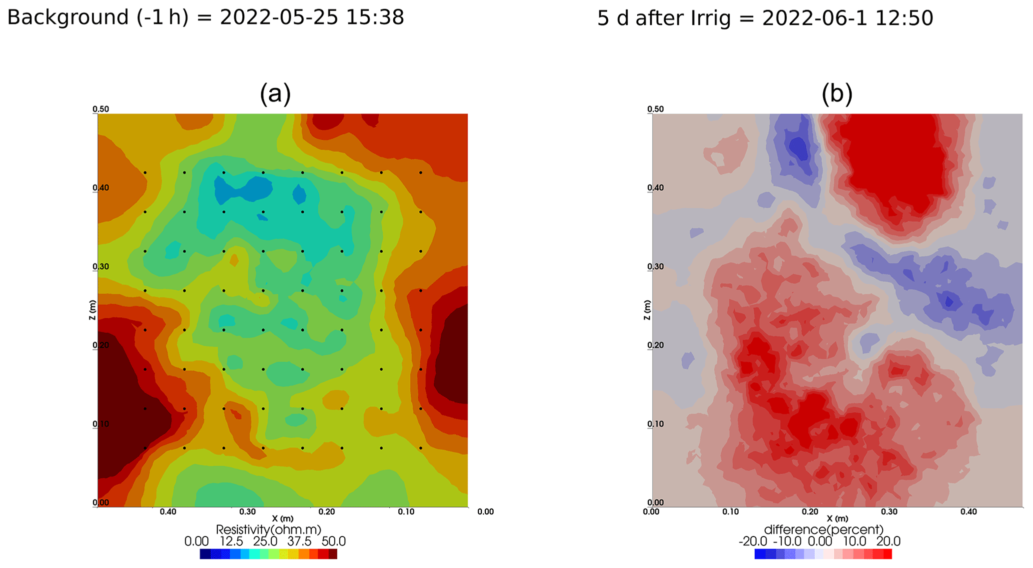
Figure A4Cycle 1 to 2 (partial irrigation: 25 May 2022, 14:30–14:15, 260 mL, through the last four upper holes (right side); no outflow through 72).
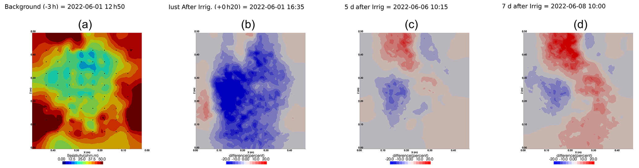
Figure A5Cycle 2 to 3 (partial irrigation: 1 June 2022, 15:50–16:10, 290 mL, through the first four upper holes (left side); no outflow through 72).
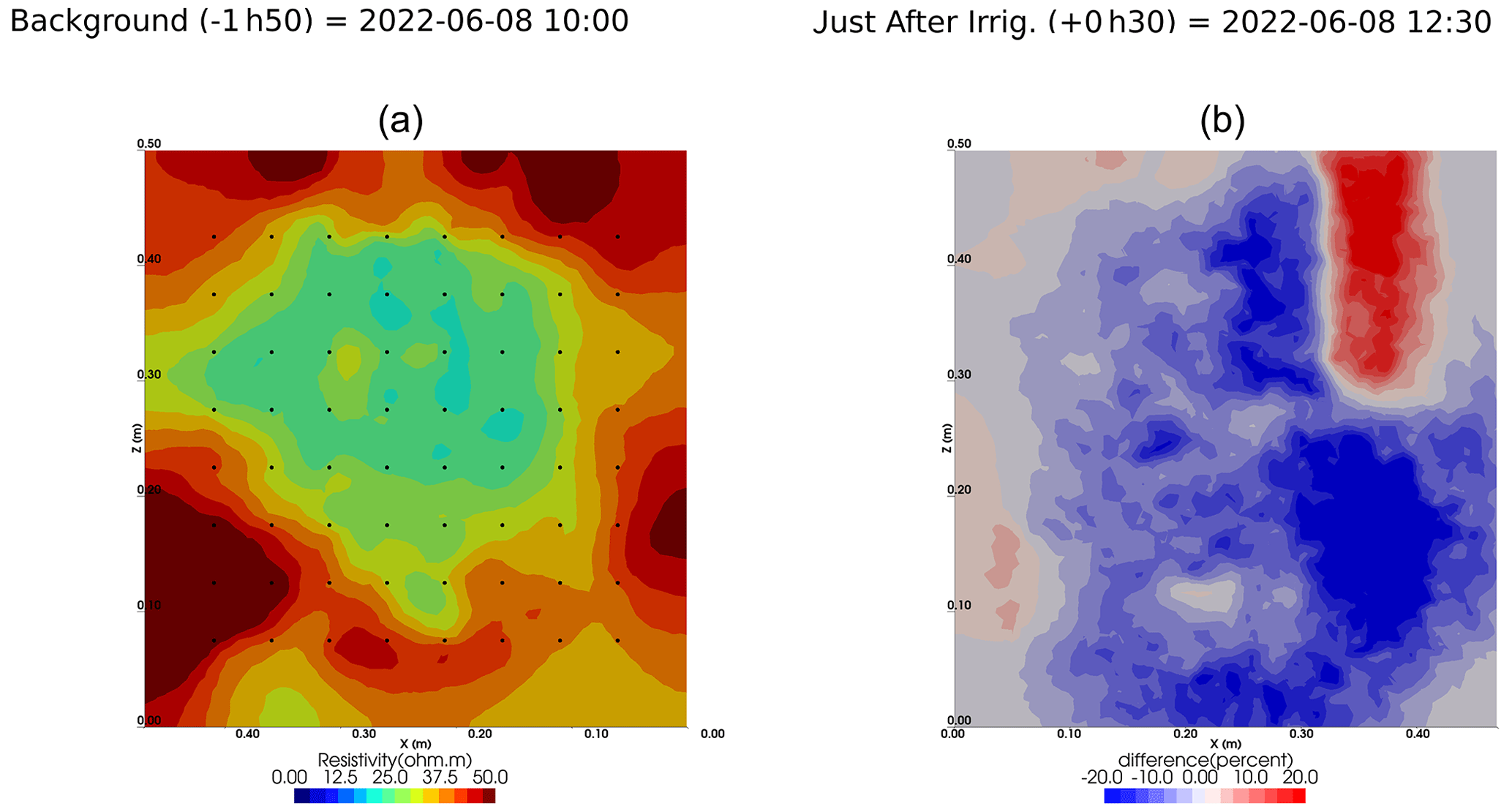
Figure A6Cycle 3 to 4 (partial irrigation: 8 June 2022, 11:50–12:00, 305 mL, through the last two upper holes (right side)).
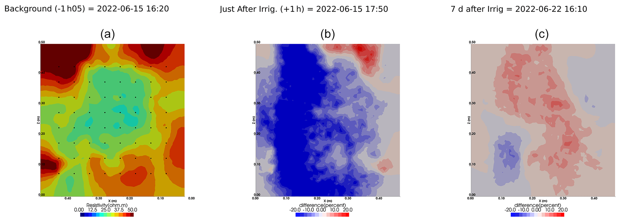
Figure A7Cycle 4 to 5 (partial irrigation: 15 June 2022, 17:25–17:45, 350 mL, through the first two upper holes (left side)).
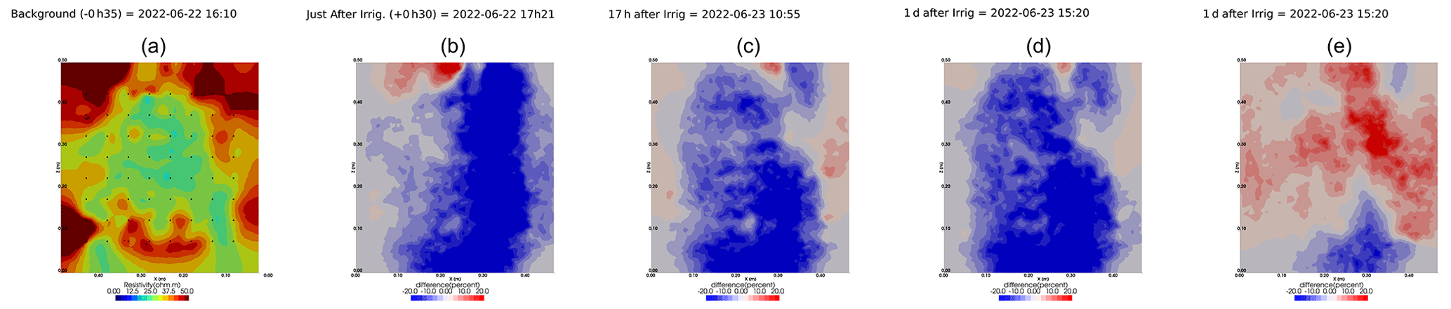
Figure A8Cycles 5 and 6 time-lapse inversion (partial right side irrigation 22 June 2022, 16:45–17:00, 375 mL).
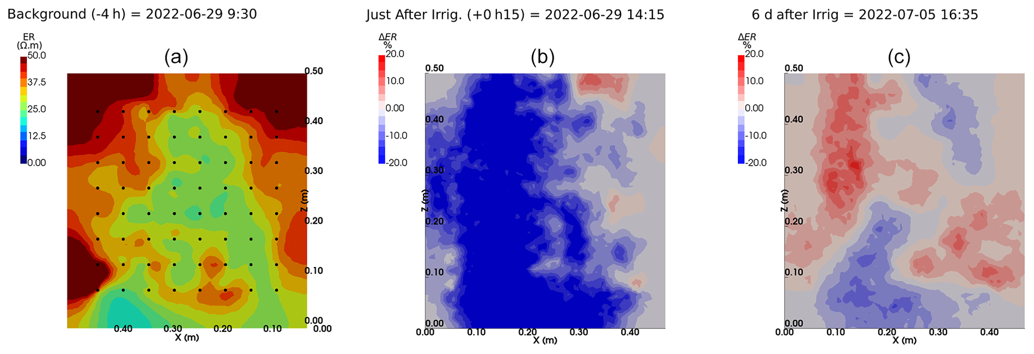
Figure A9Cycles 6 and 7 time-lapse inversion (partial left side irrigation, 29 June 2022, 13:45–14:00, 386 mL).
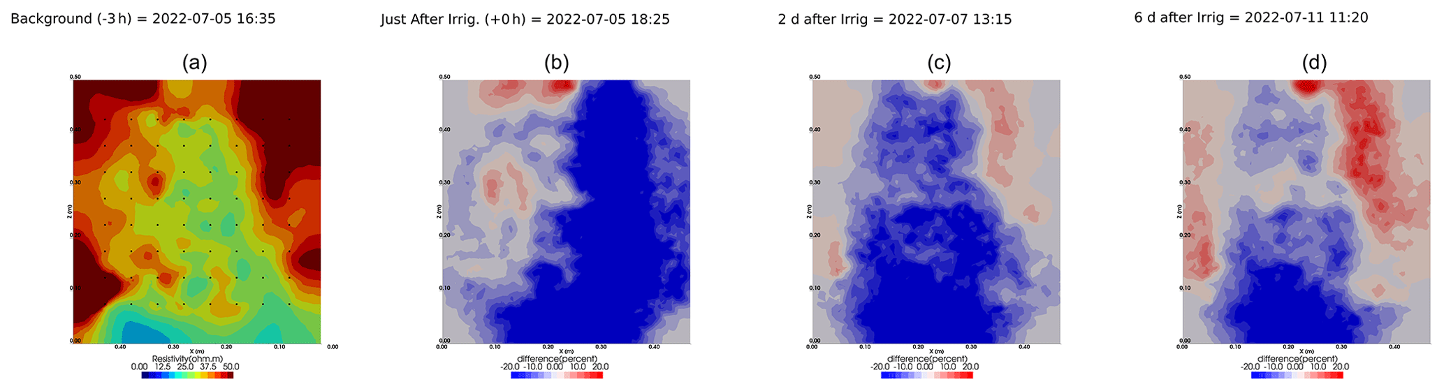
Figure A10Cycles 7 and 8 time-lapse inversion (partial right side irrigation, 5 July 2022, 18:10–18:25, 431 mL).
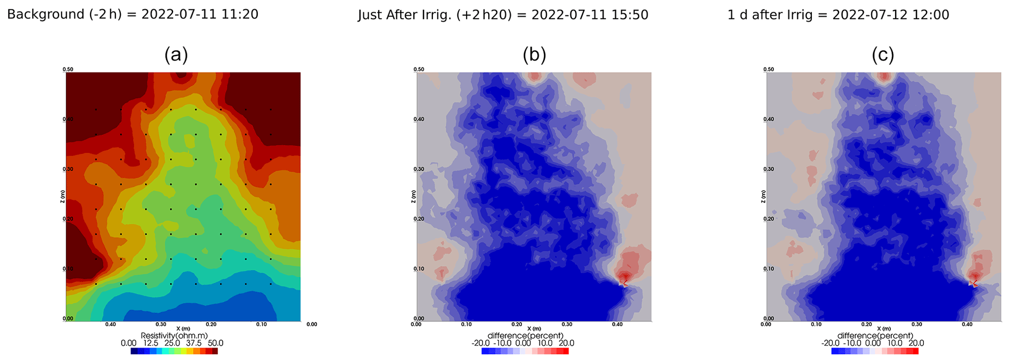
Figure A11Cycles 8 and 9 time-lapse inversion (partial right side irrigation, 11 July 2022, 13:15–13:30, 431 mL).
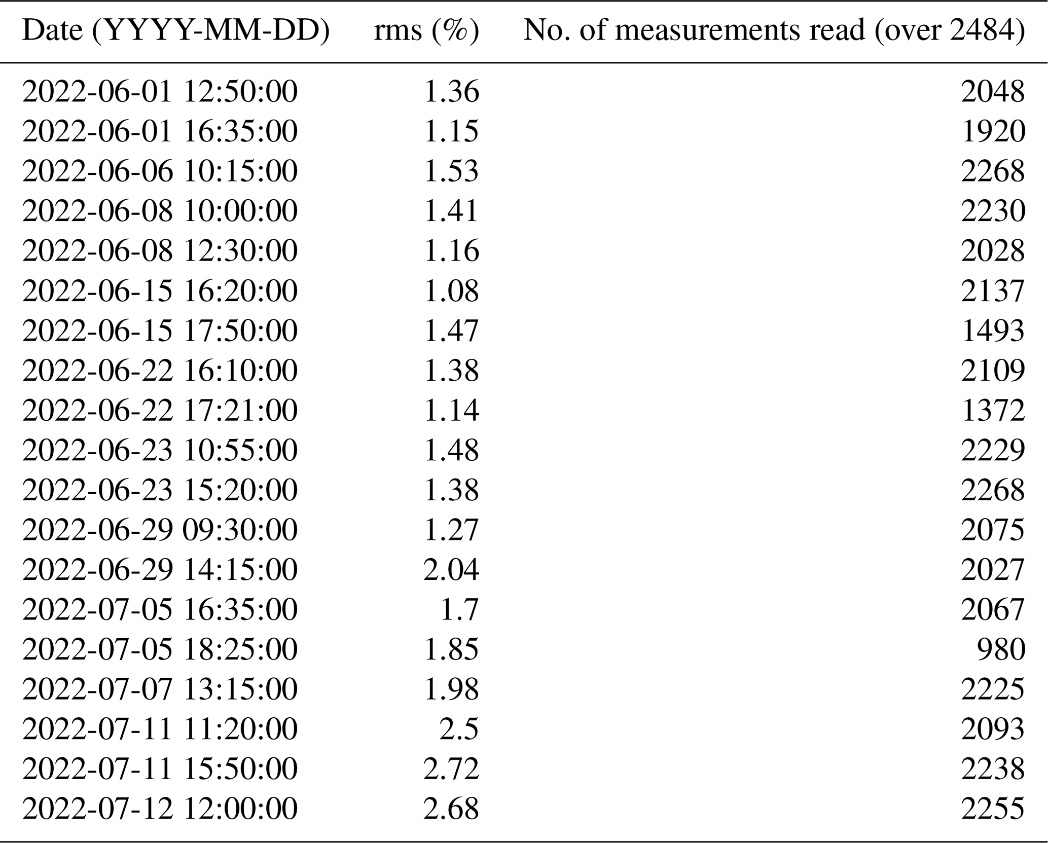
Table A1Table summarising the final rms and the number of data used for each individual inversion.
As we selected only one cycle in the paper, we report here further details about the time-lapse CSD inversion results for all the cycles. The inversion procedure is equivalent to the one described in Sect. 2.6.2 of the paper (“Analysis of current density”), and we invite the reader to consult Peruzzo et al. (2020) for a full description of the algorithm. Furthermore, we extend the analysis showing the effect of the model regularisation (smoothing). Figures B1 and B2 show the current density evolution with the time respectively for the stem and the soil injection with a regularisation parameter of 1. The same is true for Figs. B3 and B4 with a regularisation of 10.
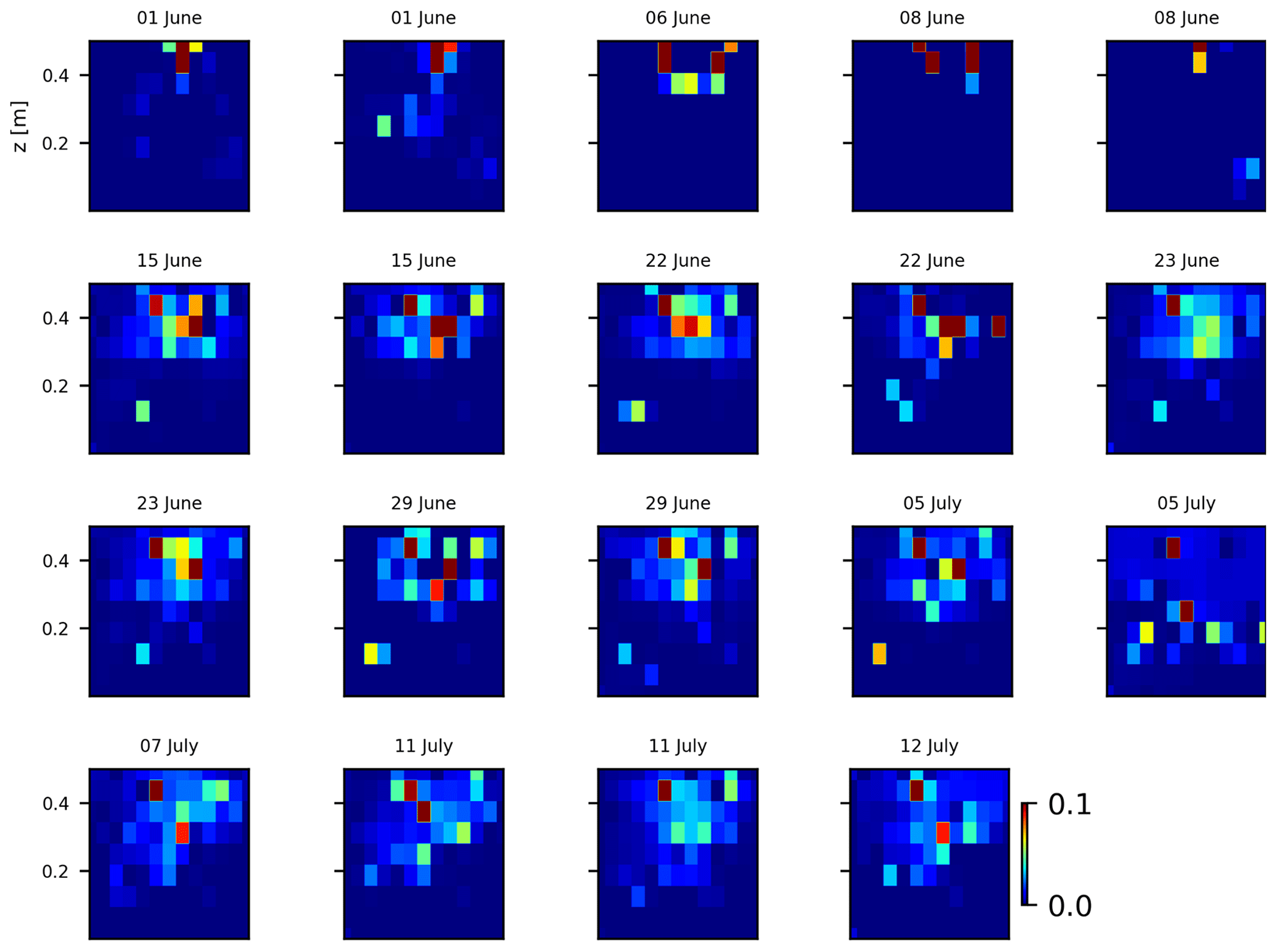
Figure B1Variations in the CSD for all the time steps (all cycles) during the stem injection. Inversion is unconstrained; the data–model weighting factor (wr) is set to 1.
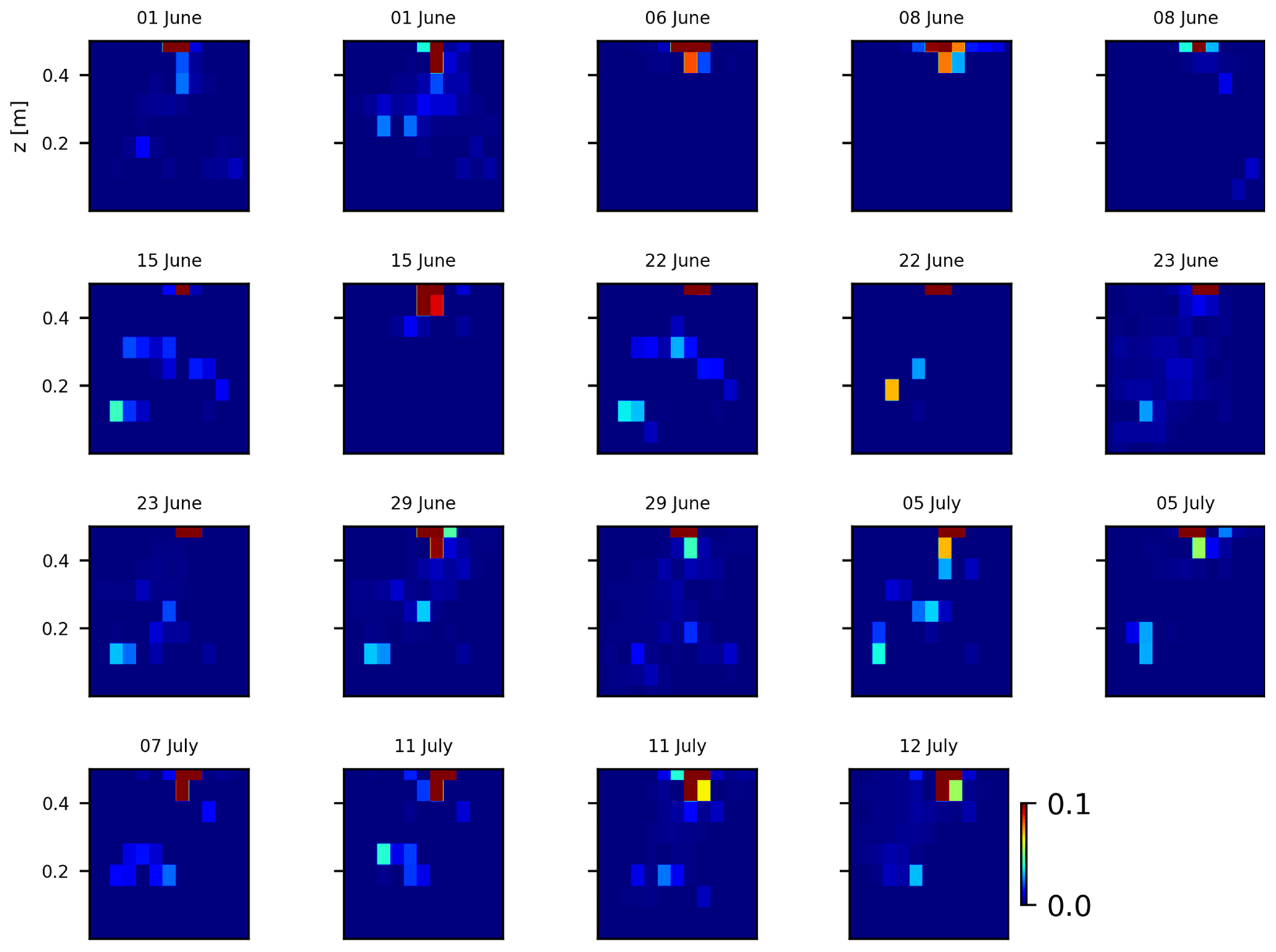
Figure B2Variations in the CSD for all the time steps (all cycles) during the soil control injection. Inversion is unconstrained; the data–model weighting factor (wr) is set to 1.
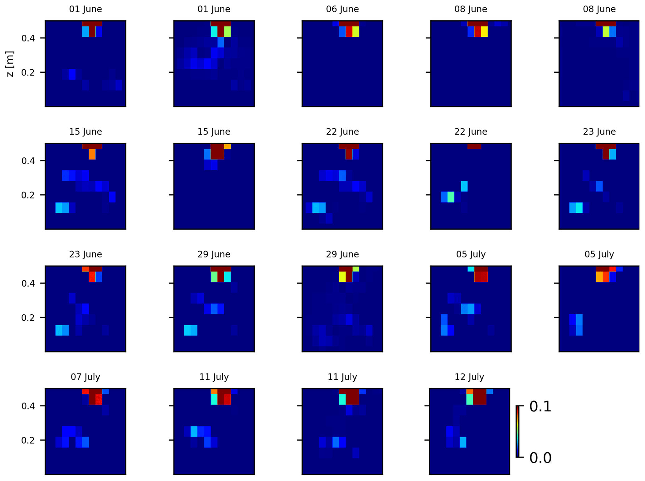
Figure B3Variations in the CSD for all the time steps (all cycles) during the soil control injection. Inversion is unconstrained; the data–model weighting factor (wr) is set to 10.
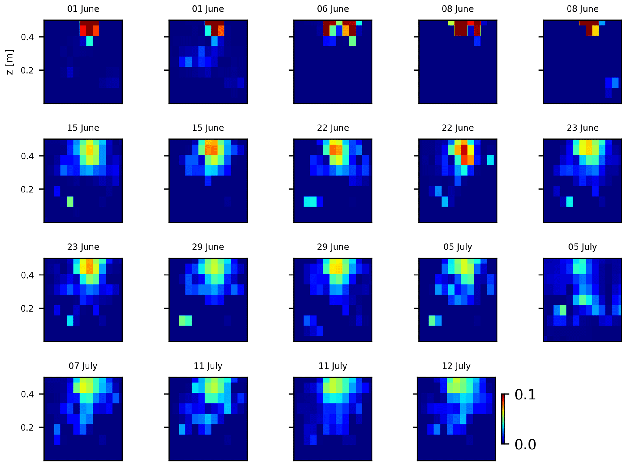
Figure B4Variations in the CSD for all the time steps (all cycles) during the stem injection. Inversion is unconstrained; the data–model weighting factor (wr) is set to 10.
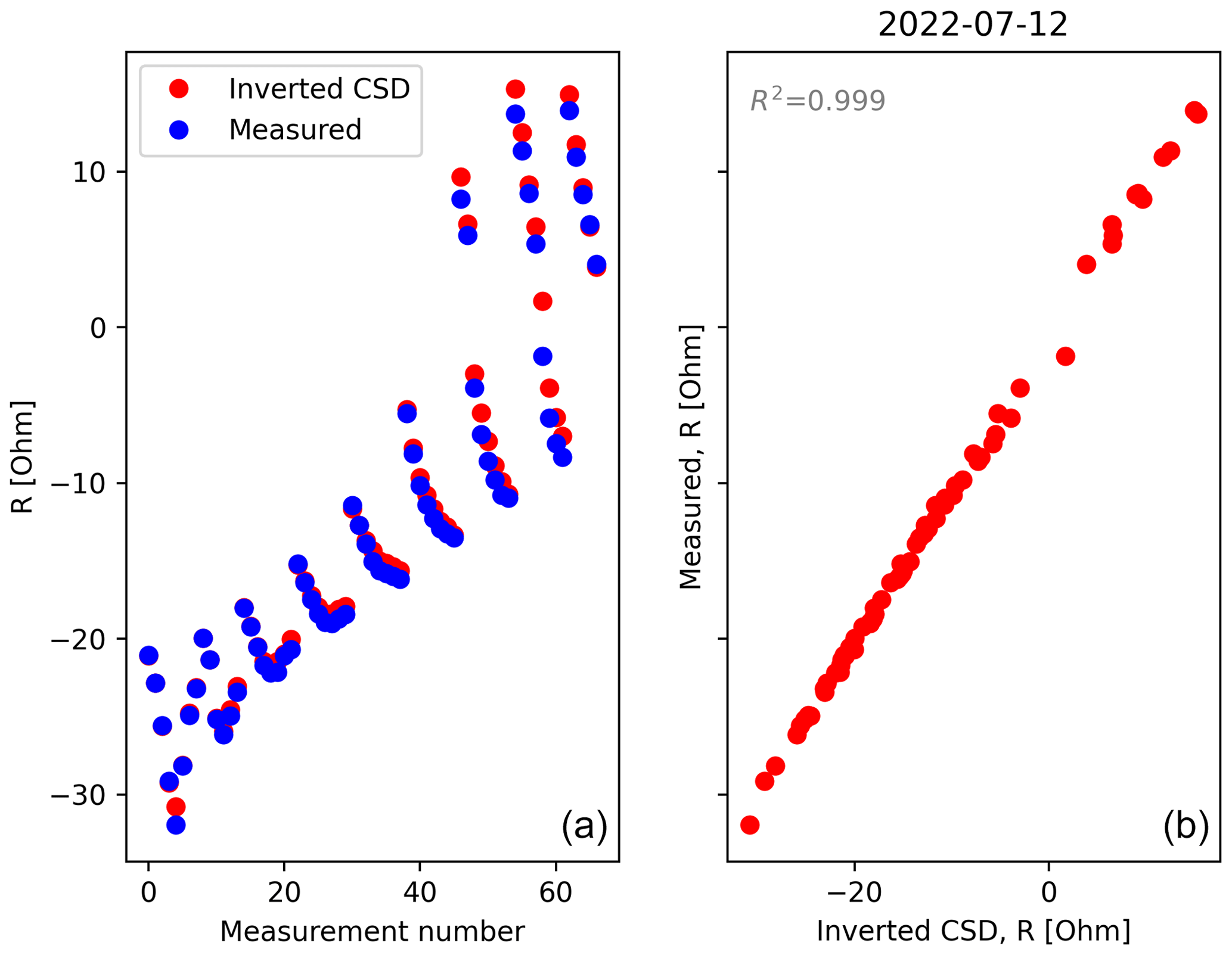
Figure B5Evaluation of the quality of the CSD inversion for the acquisition date 11 July 2022. The linear correlation coefficient is always >0.95 for all the time steps.
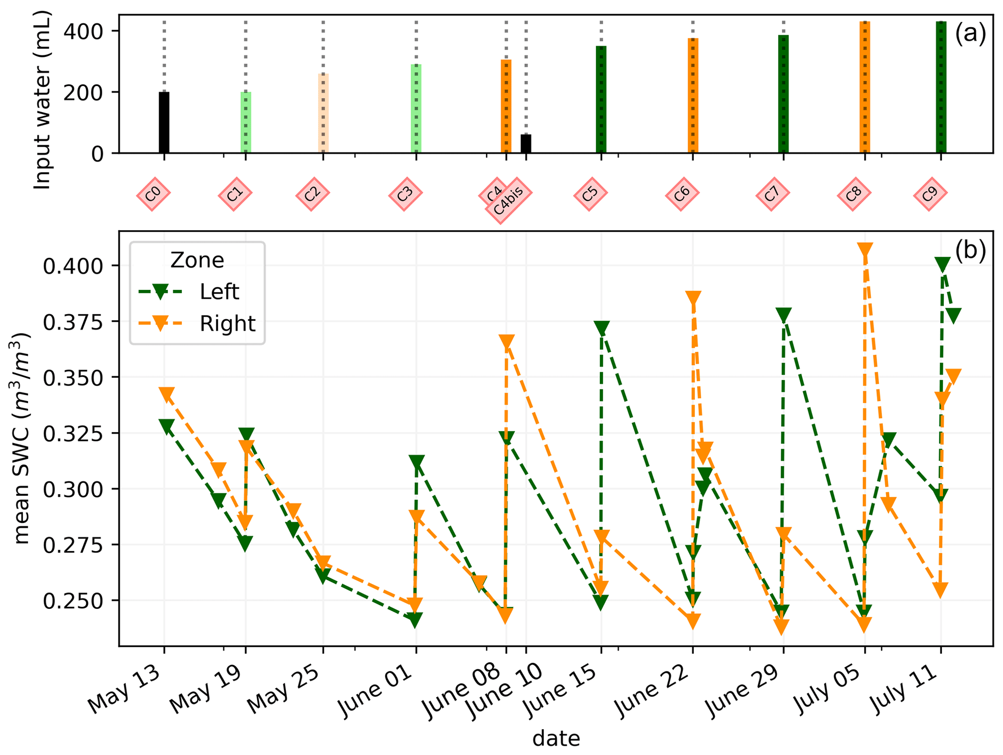
Figure C1(a) Evolution of the quantity (in mL) of water input spatially distributed with an alternation between left (green) and right (orange) during the PRD irrigation. The black bars are applicable for full-width irrigation (over all the holes; see Fig. 1), light green and orange bars are applicable for irrigation over the four sides of holes, and dark green/orange is applicable for two-hole irrigation. (b) Evolution of the mean SWC (m3 m−3) average on each side; markers show the acquisition time.
Codes and data to reproduce the figures in the paper are available in the Zenodo data repository (https://doi.org/10.5281/zenodo.10014924, Mary, 2023).
BM, VI, LP, FM, BR, CC, YW, and GB designed the experiments, and BM, VI, BR, and FM carried them out. BM, LP, GB, and CC developed the model code and performed the simulations. BM prepared the paper with contributions from all co-authors for writing (review and editing).
The contact author has declared that none of the authors has any competing interests.
Publisher's note: Copernicus Publications remains neutral with regard to jurisdictional claims made in the text, published maps, institutional affiliations, or any other geographical representation in this paper. While Copernicus Publications makes every effort to include appropriate place names, the final responsibility lies with the authors.
Benjamin Mary has been supported by the European Union's Horizon 2020 research and innovation programme under a Marie Skłodowska-Curie grant agreement (grant no. 842922).
This paper was edited by David Medvigy and reviewed by Alexandria S. Kuhl and one anonymous referee.
Abdalla, M., Carminati, A., Cai, G., Javaux, M., and Ahmed, M. A.: Stomatal closure of tomato under drought is driven by an increase in soil–root hydraulic resistance, Plant Cell Environ., 44, 425–431, https://doi.org/10.1111/pce.13939, 2021.
Anonymous Reviewer: Referee #2 comment, Comment on bg-2023-58, https://doi.org/10.5194/bg-2023-58-RC2, 2023.
Archie, G. E.: The Electrical Resistivity Log as an Aid in Determining Some Reservoir Characteristics, Trans. AIME, 146, 54–62, https://doi.org/10.2118/942054-G, 1942.
Aroca, R. and Ruiz-Lozano, J. M.: Regulation of Root Water Uptake Under Drought Stress Conditions, in: Plant Responses to Drought Stress, edited by: Aroca, R., Springer Berlin Heidelberg, Berlin, Heidelberg, 113–127, https://doi.org/10.1007/978-3-642-32653-0_4, 2012.
Binley, A.: 11.08 – Tools and Techniques: Electrical Methods, in: Treatise on Geophysics, 2nd edn., edited by: Schubert, G., Elsevier, Oxford, 233–259, https://doi.org/10.1016/B978-0-444-53802-4.00192-5, 2015.
Binley, A. and Slater, L.: Resistivity and induced polarization: theory and applications to the near-surface earth, Cambridge University Press, Cambridge, UK and New York, NY, https://doi.org/10.1007/1-4020-3102-5_5, 2020.
Blanchy, G., Saneiyan, S., Boyd, J., McLachlan, P., and Binley, A.: ResIPy, an intuitive open source software for complex geoelectrical inversion/modeling, Comput. Geosci., 137, 104423, https://doi.org/10.1016/j.cageo.2020.104423, 2020.
Cai, G., Ahmed, M. A., Abdalla, M., and Carminati, A.: Root hydraulic phenotypes impacting water uptake in drying soils, Plant Cell Environ., 45, 650–663, https://doi.org/10.1111/pce.14259, 2022.
Carminati, A. and Javaux, M.: Soil Rather Than Xylem Vulnerability Controls Stomatal Response to Drought, Trends Plant Sci., 25, 868–880, https://doi.org/10.1016/j.tplants.2020.04.003, 2020.
Cassiani, G., Boaga, J., Vanella, D., Perri, M. T., and Consoli, S.: Monitoring and modelling of soil–plant interactions: the joint use of ERT, sap flow and eddy covariance data to characterize the volume of an orange tree root zone, Hydrol. Earth Syst. Sci., 19, 2213–2225, https://doi.org/10.5194/hess-19-2213-2015, 2015.
Cassiani, G., Boaga, J., Rossi, M., Putti, M., Fadda, G., Majone, B., and Bellin, A.: Soil–plant interaction monitoring: Small scale example of an apple orchard in Trentino, North-Eastern Italy, Sci. Total Environ., 543, 851–861, https://doi.org/10.1016/j.scitotenv.2015.03.113, 2016.
Collins, M., Fuentes, S., and Barlow, E.: Partial rootzone drying and deficit irrigation increase stomatal sensitivity to vapour pressure deficit in anisohydric grapevines, Funct. Plant Biol., 37, 129–138, 2009.
Consoli, S., Stagno, F., Vanella, D., Boaga, J., Cassiani, G., and Roccuzzo, G.: Partial root-zone drying irrigation in orange orchards: Effects on water use and crop production characteristics, Eur. J. Agron., 82, 190–202, https://doi.org/10.1016/j.eja.2016.11.001, 2017.
Couvreur, V., Vanderborght, J., and Javaux, M.: A simple three-dimensional macroscopic root water uptake model based on the hydraulic architecture approach, Hydrol. Earth Syst. Sci., 16, 2957–2971, https://doi.org/10.5194/hess-16-2957-2012, 2012.
Cseresnyés, I., Vozáry, E., Kabos, S., and Rajkai, K.: Influence of substrate type and properties on root electrical capacitance, Int. Agrophys., 34, 95–101, https://doi.org/10.31545/intagr/112147, 2020.
Dalton, F. N.: In-situ root extent measurements by electrical capacitance methods, Plant Soil, 173, 157–165, https://doi.org/10.1007/BF00155527, 1995.
Davies, W. J. and Hartung, W.: Has extrapolation from biochemistry to crop functioning worked to sustain plant production under water scarcity, Conference proceedings, https://api.semanticscholar.org/CorpusID:5014928 (last access: 21 November 2023), 2004.
Davies, W. J., Wilkinson, S., and Loveys, B.: Stomatal control by chemical signalling and the exploitation of this mechanism to increase water use efficiency in agriculture, New Phytol., 153, 449–460, https://doi.org/10.1046/j.0028-646X.2001.00345.x, 2002.
Dietrich, S., Carrera, J., Weinzettel, P., and Sierra, L.: Estimation of Specific Yield and its Variability by Electrical Resistivity Tomography, Water Resour. Res., 54, 8653–8673, https://doi.org/10.1029/2018WR022938, 2018.
Dodd, I. C., Egea, G., and Davies, W. J.: Accounting for sap flow from different parts of the root system improves the prediction of xylem ABA concentration in plants grown with heterogeneous soil moisture, J. Exp. Bot., 59, 4083–4093, https://doi.org/10.1093/jxb/ern246, 2008.
Doussan, C.: Modelling of the Hydraulic Architecture of Root Systems: An Integrated Approach to Water Absorption—Distribution of Axial and Radial Conductances in Maize, Ann. Bot., 81, 225–232, https://doi.org/10.1006/anbo.1997.0541, 1998.
Doussan, C. and Garrigues, E.: Measuring and Imaging the Soil-root-water System with a Light Transmission 2D Technique, Bio-Protocol, 9, e3190, https://doi.org/10.21769/BioProtoc.3190, 2019.
Doussan, C., Vercambre, G., and Pagès, L.: Water uptake by two contrasting root systems (maize, peach tree): results from a model of hydraulic architecture, Agronomie, 19, 255–263, https://doi.org/10.1051/agro:19990306, 1999.
Düring, H., Dry, P. R., Botting, D. G., and Loveys, B.: Effects of partial root-zone drying on grapevine vigour, yield, composition of fruit and use of water, in: Proceedings of the Ninth Australian Wine Industry Technical Conference, Adelaide, South Australia, 16–19 July 1995, 128–131, 1996.
Ehosioke, S., Nguyen, F., Rao, S., Kremer, T., Placencia-Gomez, E., Huisman, J. A., Kemna, A., Javaux, M., and Garré, S.: Sensing the electrical properties of roots: A review, Vadose Zone J., 19, e20082, https://doi.org/10.1002/vzj2.20082, 2020.
Elsner, E. A. and Jubb, G. L.: Leaf Area Estimation of Concord Grape Leaves from Simple Linear Measurements, Am. J. Enol. Viticult., 39, 95–97, 1988.
Fernández, J. E., Díaz-Espejo, A., Infante, J. M., Durán, P., Palomo, M. J., Chamorro, V., Girón, I. F., and Villagarcía, L.: Water relations and gas exchange in olive trees under regulated deficit irrigation and partial rootzone drying, Plant Soil, 284, 273–291, https://doi.org/10.1007/s11104-006-0045-9, 2006.
Frensch, J. and Steudle, E.: Axial and Radial Hydraulic Resistance to Roots of Maize (Zea mays L.), Plant Physiol., 91, 719–726, https://doi.org/10.1104/pp.91.2.719, 1989.
Garré, S., Javaux, M., Vanderborght, J., Pagès, L., and Vereecken, H.: Three-dimensional electrical resistivity tomography to monitor root zone water dynamics, Vadose Zone J., 10, 412–424, https://doi.org/10.2136/vzj2010.0079, 2011.
Garré, S., Hyndman, D., Mary, B., and Werban, U.: Geophysics conquering new territories: The rise of “agrogeophysics,” Vadose Zone J., 20, e20115, https://doi.org/10.1002/vzj2.20115, 2021.
Garrigues, E., Doussan, C., and Pierret, A.: Water Uptake by Plant Roots: I – Formation and Propagation of a Water Extraction Front in Mature Root Systems as Evidenced by 2D Light Transmission Imaging, Plant Soil, 283, 83–98, https://doi.org/10.1007/s11104-004-7903-0, 2006.
Geuzaine, C. and Remacle, J.-F.: Gmsh: A 3-D finite element mesh generator with built-in pre- and post-processing facilities, Int. J. Numer. Meth. Eng., 79, 1309–1331, https://doi.org/10.1002/nme.2579, 2009.
Gibert, D., Le Mouël, J.-L., Lambs, L., Nicollin, F., and Perrier, F.: Sap flow and daily electric potential variations in a tree trunk, Plant Sci., 171, 572–584, https://doi.org/10.1016/j.plantsci.2006.06.012, 2006.
Gimenez, C., Gallardo, M., and Thompson, R. B.: Plant–Water Relations, in: Encyclopedia of Soils in the Environment, edited by: Hillel, D., Elsevier, Oxford, 231–238, https://doi.org/10.1016/B0-12-348530-4/00459-8, 2005.
Gu, H., Liu, L., Butnor, J., Sun, H., Zhang, X., Li, C., and Liu, X.: Electrical capacitance estimates crop root traits best under dry conditions – a case study in cotton (Gossypium hirsutum L.), Plant Soil, 467, 1–19, https://doi.org/10.1007/s11104-021-05094-6, 2021.
Hoagland, D. R. and Arnon, D. I.: The water culture method for growing plants without soil, California Agric. Exp. Stn. Circ., 347, 1–32, 1950.
Jackisch, C., Knoblauch, S., Blume, T., Zehe, E., and Hassler, S. K.: Estimates of tree root water uptake from soil moisture profile dynamics, Biogeosciences, 17, 5787–5808, https://doi.org/10.5194/bg-17-5787-2020, 2020.
Javaux, M., Schröder, T., Vanderborght, J., and Vereecken, H.: Use of a Three‐Dimensional Detailed Modeling Approach for Predicting Root Water Uptake, Vadose Zone J., 7, 1079–1088, https://doi.org/10.2136/vzj2007.0115, 2008.
Kamarajan, C., Pandey, A. K., Chorlian, D. B., and Porjesz, B.: The use of current source density as electrophysiological correlates in neuropsychiatric disorders: a review of human studies, Int. J. Psychophysiol., 97, 310–322, https://doi.org/10.1016/j.ijpsycho.2014.10.013, 2015.
Liu, Y., Li, D., Qian, J., Di, B., Zhang, G., and Ren, Z.: Electrical impedance spectroscopy (EIS) in plant roots research: a review, Plant Methods, 17, 118, https://doi.org/10.1186/s13007-021-00817-3, 2021.
Loveys, B. R., Dry, P. R., Stoll, M., and McCarthy, M. G.: USING PLANT PHYSIOLOGY TO IMPROVE THE WATER USE EFFICIENCY OF HORTICULTURAL CROPS, Acta Hortic., 537, 187–197, https://doi.org/10.17660/ActaHortic.2000.537.19, 2000.
Lovisolo, C., Lavoie-Lamoureux, A., Tramontini, S., and Ferrandino, A.: Grapevine adaptations to water stress: new perspectives about soil/plant interactions, Theor. Exp. Plant Phys., 28, 53–66, https://doi.org/10.1007/s40626-016-0057-7, 2016.
Malavasi, U. C., Davis, A. S., and Malavasi, M. de M.: Lignin in Woody Plants under Water Stress: A Review, Floresta E Ambiente, 23, 589–597, https://doi.org/10.1590/2179-8087.143715, 2016.
Mancuso, S. (Ed.): Measuring roots: an updated approach, Springer, Heidelberg, New York, 382 pp., ISBN 978-3-642-22067-8, 2012.
Manoli, G., Bonetti, S., Domec, J.-C., Putti, M., Katul, G., and Marani, M.: Tree root systems competing for soil moisture in a 3D soil–plant model, Adv. Water Resour., 66, 32–42, https://doi.org/10.1016/j.advwatres.2014.01.006, 2014.
Martin-Vertedor, A. I. and Dodd, I. C.: Root-to-shoot signalling when soil moisture is heterogeneous: increasing the proportion of root biomass in drying soil inhibits leaf growth and increases leaf abscisic acid concentration: Root distribution and non-hydraulic signalling, Plant Cell Environ., 34, 1164–1175, https://doi.org/10.1111/j.1365-3040.2011.02315.x, 2011.
Mary, B.: Codes and data to reproduce figures articles are available in the Zenodo data repository, Zenodo [code, data set], https://doi.org/10.5281/zenodo.10014924, 2023.
Mary, B., Peruzzo, L., Boaga, J., Schmutz, M., Wu, Y., Hubbard, S. S., and Cassiani, G.: Small-scale characterization of vine plant root water uptake via 3-D electrical resistivity tomography and mise-à-la-masse method, Hydrol. Earth Syst. Sci., 22, 5427–5444, https://doi.org/10.5194/hess-22-5427-2018, 2018.
Mary, B., Rao, S., Javaux, M., and Cassiani, G.: Tree root system mise-à-la-masse (MALM) forward modelling with explicit representation of root structure, Geophys. Res. Abstr., EGU2019-4940, EGU General Assembly 2019, Vienna, Austria, 2019a.
Mary, B., Vanella, D., Consoli, S., and Cassiani, G.: Assessing the extent of citrus trees root apparatus under deficit irrigation via multi-method geo-electrical imaging, Sci. Rep.-UK, 9, 9913, https://doi.org/10.1038/s41598-019-46107-w, 2019b.
McAdam, S. A. M., Sussmilch, F. C., and Brodribb, T. J.: Stomatal responses to vapour pressure deficit are regulated by high speed gene expression in angiosperms, Plant Cell Environ., 39, 485–491, https://doi.org/10.1111/pce.12633, 2016.
Michot, D., Benderitter, Y., Dorigny, A., Nicoullaud, B., King, D., and Tabbagh, A.: Spatial and temporal monitoring of soil water content with an irrigated corn crop cover using surface electrical resistivity tomography: Soil Water Study Using Electrical Resistivity, Water Resour. Res., 39, 1138, https://doi.org/10.1029/2002WR001581, 2003.
Mingo, D. M., Bacon, M. A., and Davies, W. J.: Non‐hydraulic regulation of fruit growth in tomato plants (Lycopersicon esculentum cv. Solairo) growing in drying soil, J. Exp. Bot., 54, 1205–1212, https://doi.org/10.1093/jxb/erg120, 2003.
Parsekian, A. D., Claes, N., Singha, K., Minsley, B. J., Carr, B., Voytek, E., Harmon, R., Kass, A., Carey, A., Thayer, D., and Flinchum, B.: Comparing Measurement Response and Inverted Results of Electrical Resistivity Tomography Instruments, J. Environ. Eng. Geoph., 22, 249–266, https://doi.org/10.2113/JEEG22.3.249, 2017.
Peruzzo, L., Chou, C., Wu, Y., Schmutz, M., Mary, B., Wagner, F. M., Petrov, P., Newman, G., Blancaflor, E. B., Liu, X., Ma, X., and Hubbard, S.: Imaging of plant current pathways for non-invasive root Phenotyping using a newly developed electrical current source density approach, Plant Soil, 450, 567–584, https://doi.org/10.1007/s11104-020-04529-w, 2020.
Peruzzo, L., Liu, X., Chou, C., Blancaflor, E. B., Zhao, H., Ma, X.-F., Mary, B., Iván, V., Weigand, M., and Wu, Y.: Three-channel electrical impedance spectroscopy for field-scale root phenotyping, Plant Phenome J., 4, e20021, https://doi.org/10.1002/ppj2.20021, 2021.
Postic, F. and Doussan, C.: Benchmarking electrical methods for rapid estimation of root biomass, Plant Methods, 12, 33, https://doi.org/10.1186/s13007-016-0133-7, 2016.
Rao, S., Meunier, F., Ehosioke, S., Lesparre, N., Kemna, A., Nguyen, F., Garré, S., and Javaux, M.: A mechanistic model for electrical conduction in soil–root continuum: a virtual rhizotron study, Biogeosciences Discuss. [preprint], https://doi.org/10.5194/bg-2018-280, 2018.
Sartoni, R., Zegada-Lizarazu, W., and Monti, A.: A new compartmentalised rhizotron system for root phenotyping, Ital. J. Agron., 10, 53, https://doi.org/10.4081/ija.2015.645, 2015.
Sharp, R. E. and Davies, W. J.: Regulation of growth and development of plants growing with a restricted supply of water, Soc. Exp. Biol. Sem. Ser., 77–93, ISBN 978-0-521-05037-1, 1989.
Smart, D. R., Carlisle, E., Goebel, M., and Nunez, B. A.: Transverse hydraulic redistribution by a grapevine, Plant Cell Environ., 28, 157–166, https://doi.org/10.1111/j.1365-3040.2004.01254.x, 2005.
Song, C., Shen, W., Du, L., Wen, J., Lin, J., and Li, R.: Development and chemical characterization of Casparian strips in the roots of Chinese fir (Cunninghamia lanceolata), Trees, 33, 827–836, https://doi.org/10.1007/s00468-019-01820-x, 2019.
Srayeddin, I. and Doussan, C.: Estimation of the spatial variability of root water uptake of maize and sorghum at the field scale by electrical resistivity tomography, Plant Soil, 319, 185–207, https://doi.org/10.1007/s11104-008-9860-5, 2009.
Stoll, M.: Effects of partial rootzone drying on grapevine physiology and fruit quality, Adelaide University, https://hdl.handle.net/2440/37734 (last access: 21 November 2023), 2000.
Stoll, M., Loveys, B., and Dry, P.: Hormonal changes induced by partial rootzone drying of irrigated grapevine, J. Exp. Bot., 51, 1627–1634, https://doi.org/10.1093/jexbot/51.350.1627, 2000.
Taylor, H. M., Upchurch, D. R., and McMichael, B. L.: Applications and limitations of rhizotrons and minirhizotrons for root studies, Plant Soil, 129, 29–35, https://doi.org/10.1007/BF00011688, 1990.
Tsialtas, J. T., Koundouras, S., and Zioziou, E.: Leaf area estimation by simple measurements and evaluation of leaf area prediction models in Cabernet-Sauvignon grapevine leaves, Photosynthetica, 46, 452–456, https://doi.org/10.1007/s11099-008-0077-x, 2008.
Tsukanov, K. and Schwartz, N.: Relationship between wheat root properties and its electrical signature using the spectral induced polarization method, Vadose Zone J., 19, e20014, https://doi.org/10.1002/vzj2.20014, 2020.
Tsukanov, K. and Schwartz, N.: Modeling Plant Roots Spectral Induced Polarization Signature, Geophys. Res. Lett., 48, e2020GL090184, https://doi.org/10.1029/2020GL090184, 2021.
Uhlemann, S., Wilkinson, P. B., Maurer, H., Wagner, F. M., Johnson, T. C., and Chambers, J. E.: Optimized survey design for electrical resistivity tomography: combined optimization of measurement configuration and electrode placement, Geophys. J. Int., 214, 108–121, https://doi.org/10.1093/gji/ggy128, 2018.
Urban, J., Bequet, R., and Mainiero, R.: Assessing the applicability of the earth impedance method for in situ studies of tree root systems, J. Exp. Bot., 62, 1857–1869, https://doi.org/10.1093/jxb/erq370, 2011.
Vanella, D., Cassiani, G., Busato, L., Boaga, J., Barbagallo, S., Binley, A., and Consoli, S.: Use of small scale electrical resistivity tomography to identify soil-root interactions during deficit irrigation, J. Hydrol., 556, 310–324, https://doi.org/10.1016/j.jhydrol.2017.11.025, 2018.
Virtanen, P., Gommers, R., Oliphant, T. E., Haberland, M., Reddy, T., Cournapeau, D., Burovski, E., Peterson, P., Weckesser, W., Bright, J., van der Walt, S. J., Brett, M., Wilson, J., Millman, K. J., Mayorov, N., Nelson, A. R. J., Jones, E., Kern, R., Larson, E., Carey, C. J., Polat, İ., Feng, Y., Moore, E. W., VanderPlas, J., Laxalde, D., Perktold, J., Cimrman, R., Henriksen, I., Quintero, E. A., Harris, C. R., Archibald, A. M., Ribeiro, A. H., Pedregosa, F., and van Mulbregt, P.: SciPy 1.0: fundamental algorithms for scientific computing in Python, Nat. Methods, 17, 261–272, https://doi.org/10.1038/s41592-019-0686-2, 2020.
Voytek, E. B., Barnard, H. R., Jougnot, D., and Singha, K.: Transpiration- and precipitation-induced subsurface water flow observed using the self-potential method, Hydrol. Process., 33, 1784–1801, https://doi.org/10.1002/hyp.13453, 2019.
Whalley, W. R., Binley, A., Watts, C. W., Shanahan, P., Dodd, I. C., Ober, E. S., Ashton, R. W., Webster, C. P., White, R. P., and Hawkesford, M. J.: Methods to estimate changes in soil water for phenotyping root activity in the field, Plant Soil, 415, 407–422, https://doi.org/10.1007/s11104-016-3161-1, 2017.
Weigand, M.: Monitoring Structural And Physiological Properties Of Crop Roots Using Spectral Electrical Impedance Tomography, Dissertation, University of Bonn, https://nbn-resolving.org/urn:nbn:de:hbz:5n-46750 (last access: 21 November 2023), 2017.
Weigand, M. and Kemna, A.: Imaging and functional characterization of crop root systems using spectroscopic electrical impedance measurements, Plant Soil, 435, 201–224, https://doi.org/10.1007/s11104-018-3867-3, 2019.
Yan, J., Bogie, N. A., and Ghezzehei, T. A.: Root uptake under mismatched distributions of water and nutrients in the root zone, Biogeosciences, 17, 6377–6392, https://doi.org/10.5194/bg-17-6377-2020, 2020.
- Abstract
- Introduction
- Material and methods
- Results
- Discussion
- Conclusion
- Appendix A: Time-lapse ERT inversion results
- Appendix B: Inversion of current density (CSD)
- Appendix C: Soil water content converted variations
- Code and data availability
- Author contributions
- Competing interests
- Disclaimer
- Financial support
- Review statement
- References