Temporal variability of observed and simulated gross primary productivity, modulated by vegetation state and hydrometeorological drivers

The gross primary production (GPP) of the terrestrial biosphere is a key source of variability in the global carbon cycle. It is modulated by hydrometeorological drivers (i.e. short-wave radiation, air temperature, vapour pressure deficit and soil moisture) and the vegetation state (i.e. canopy greenness, leaf area index) at instantaneous to interannual timescales. In this study, we set out to evaluate the ability of GPP models to capture this variability. Eleven models were considered, which rely purely on remote sensing data (RS-driven), meteorological data (meteo-driven, e.g. dynamic global vegetation models; DGVMs) or a combination of both (hybrid, e.g. light-use efficiency, LUE, models). They were evaluated using in situ observations at 61 eddy covariance sites, covering a broad range of herbaceous and forest biomes.

The results illustrated how the determinant of temporal variability shifts from meteorological variables at sub-seasonal timescales to biophysical variables at seasonal and interannual timescales. RS-driven models lacked the sensitivity to the dominant drivers at short timescales (i.e. short-wave radiation and vapour pressure deficit) and failed to capture the decoupling of photosynthesis and canopy greenness (e.g. in evergreen forests). Conversely, meteo-driven models accurately captured the variability across timescales, despite the challenges in the prognostic simulation of the vegetation state. The largest errors were found in water-limited sites, where the accuracy of the soil moisture dynamics determines the quality of the GPP estimates. In arid herbaceous sites, canopy greenness and photosynthesis were more tightly coupled, resulting in improved results with RS-driven models. Hybrid models capitalized on the combination of RS observations and meteorological information. LUE models were among the most accurate models to monitor GPP across all biomes, despite their simple architecture.

Overall, we conclude that the combination of meteorological drivers and remote sensing observations is required to yield an accurate reproduction of the spatio-temporal variability of GPP. To further advance the performance of DGVMs, improvements in the soil moisture dynamics and vegetation evolution are needed.

1 Introduction

Within the global carbon cycle, the exchange of carbon via photosynthesis and respiration in the terrestrial biosphere represents one of the largest and most dynamic components. Roughly 130 Pg C yr⁻¹ flows through plant stomata for gross primary productivity (GPP), from the total 875 Pg C stored in the atmosphere (IPCC, 2013; Friedlingstein et al., 2022). During the decade 2012–2021, 3.1 ± 0.6 Pg C yr⁻¹ was captured in the net terrestrial biosphere sink (i.e. gross primary productivity minus ecosystem respiration). With an interannual variability of 1 Pg C yr⁻¹, it is considered the most variable element in the global carbon cycle (Friedlingstein et al., 2022). Despite the substantial role of GPP in the global carbon cycle, quantifying this flux is still associated with large uncertainties (Anav et al., 2015).

The temporal variability of GPP is largely modulated by the vegetation state (i.e. canopy greenness, leaf area index, etc.) and hydrometeorological conditions (Beer et al., 2010; Delpierre et al., 2012; Anav et al., 2015; Baldocchi et al., 2018). Consequently, most GPP models rely on remotely sensed (RS) observations of the vegetation, meteorological forcings, or a combination thereof (Xiao et al., 2019; Friedlingstein et al., 2022; Jung et al., 2020). The vegetation state can be observed via remote sensing, making it an attractive approach to estimate global GPP dynamics. Vegetation indices (VIs), such as the normalized difference vegetation index (NDVI; Rouse et al., 1974), enhanced vegetation index (EVI; Huete et al., 2002) or near-infrared reflectance of vegetation (NIRv; Badgley et al., 2017), are indicators of the presence of (green) vegetation. Given their robustness and the availability of relatively long time series, the potential of these VIs as a (linear) proxy for GPP has been explored by various studies (Tucker et al., 1986; Xiao et al., 2019; Huang et al., 2019; Balzarolo et al., 2019). Advancing beyond this, machine learning methods have been used to better exploit the potential of optical RS data in the recent decade (e.g. FluxCom; Jung et al., 2020), and the potential of new RS proxies with a more direct link to photosynthesis has been established, e.g. solar-induced chlorophyll fluorescence (SIF; Frankenberg et al., 2011; Liu et al., 2017; Pickering et al., 2022). The challenge associated with these models is that the relation between vegetation state and photosynthesis can decouple due to other limiting factors, such as soil moisture, temperature and short-wave radiation (Walther et al., 2016; Hu et al., 2022).

Unlike RS-driven models, dynamic global vegetation models (DGVMs) are driven largely by meteorological forcings. They are process-based models in which the exchanges of energy, water, and carbon between the terrestrial biosphere and the atmosphere are simulated in a mechanistic manner. These models allow one to assess the terrestrial carbon assimilation in the global carbon budget or to investigate historic and future trends under a changing climate (Friedlingstein et al., 2022). The key challenge in these highly complex models is the correct representation of all underlying processes, including the dynamics of the canopy (Sitch et al., 2015; Fatichi et al., 2019). The entangled nature of these processes and the resulting disagreements in the model conceptualizations contribute to the large spread between these models and uncertainty associated with the land surface sink in earth system models (Haughton et al., 2016; Collier et al., 2018; Seiler et al., 2022).

In the frame of this study, hybrid models are models that rely on a combination of RS observations of the vegetation state and meteorological forcings. The light-use efficiency (LUE) model, proposed by Monteith (1972), is one of the most elementary formulations. Thanks to its compatibility with RS observations and limited input requirements, this semi-mechanistic approach is widely used and available in many flavours and degrees of complexity (Pei et al., 2022). Examples include the MODIS MOD17 GPP product (Running et al., 2004) or the LSA SAF GPP product (Satellite Application Facility on Land Surface Analysis; Martínez et al., 2020). These models benefit from the complementary information in RS data and meteorological forcings but remain sensitive to uncertainties associated with RS observations of dense vegetation and the incomplete representation of soil moisture stress (Stocker et al., 2018; Xiao et al., 2019; Bloomfield et al., 2023).

The impact of vegetation and hydrometeorological conditions on the temporal variability of GPP ranges from instantaneous to interannual timescales (Stoy et al., 2009; Mahecha et al., 2010; Linscheid et al., 2020). As the available GPP models vary in architecture, in the representation of underlying processes (or absence thereof) and – eminently – in their forcings, their shortcomings vary across biomes and temporal scales (Anav et al., 2015; Mahecha et al., 2010; Xiao et al., 2019). Depending on their application, models are required to give a good estimate of annual variability, response to climate extremes or changes in phenology. In order to adequately capture these temporal patterns, the timescale-dependent sensitivity of GPP to its drivers needs to be represented accurately (Delpierre et al., 2012; Linscheid et al., 2021). Model evaluation studies or intercomparison studies are in this regard generally restricted to a single model type (RS-driven, meteo-driven or hybrid), driver and/or timescale (Mahecha et al., 2010; Delpierre et al., 2012; Shao et al., 2015). Despite important efforts made in this domain, most notably with the International Land Model Benchmarking system (ILAMB; Collier et al., 2018), it remains currently largely unclear what the inter-model trade-offs are.

The overall objective of this study is to evaluate the ability of various modelling approaches (RS-driven, meteo-driven or hybrid) to capture the temporal variability of GPP. By comparing the simulations of GPP with in situ eddy covariance observations, we aim to assess (1) their performance across a broad range of biomes and temporal scales and (2) their sensitivity to drivers of GPP (i.e. vegetation state and hydrometeorological conditions).

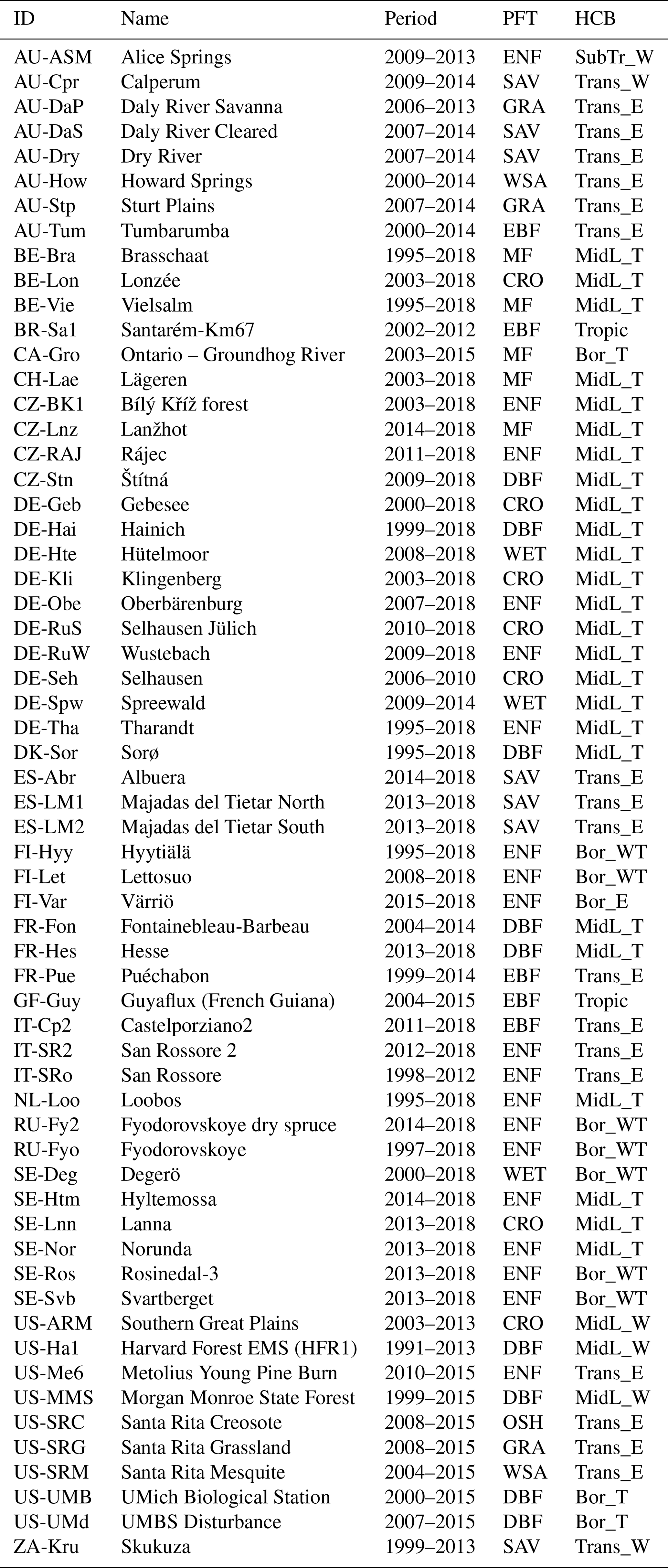
Table 1 Selection of 61 FLUXNET/ICOS (Integrated Carbon Observation System) sites used in this study. Classification by plant functional type (PFT; evergreen broadleaf forest: EBF, evergreen needleleaf forest: ENF, deciduous broadleaf forest: DBF, mixed forest: MF, wetland: WET, grassland: GRA, open shrubland: OSH, savanna: SAV, woody savanna: WSA, cropland: CRO) and hydroclimatic biome (HCB; Boreal/Mid-Latitude/Transitional/Subtropical/Tropical + Energy/Water/Temperature-driven; Papagiannopoulou et al., 2018). Note that only data beginning from 2007 were used in this study. All sites with data until 2018 are taken from the ICOS 2018 drought initiative; data for the other sites were collected from the FLUXNET2015 dataset.

2 Materials and methods

2.1 Test sites

The evaluation of the GPP models was performed using in situ observations from eddy covariance stations. Test sites were selected from the FLUXNET2015 dataset (Pastorello et al., 2020) and the ICOS “2018 drought initiative” dataset (Drought 2018 Team and ICOS Ecosystem Thematic Centre, 2019). It was ensured that the sites had a homogeneous land cover, which could be captured by the remote sensing products. A site was considered homogeneous when in 1 km × 1 km area surrounding the station location was dominated by a unique vegetation type (i.e. grassland, deciduous forest, evergreen forest). The site homogeneity was visually evaluated using high-resolution satellite images in Google Earth. Additionally, the sites were required to have a minimum of 3 years of GPP data since 1 January 2007 (i.e. the start of the SIF time series). This resulted in a selection of 61 sites, listed in Table 1. The dataset contained 461 years worth of GPP data, in which evergreen needleleaf forest (ENF) and the mid-latitude temperature-driven hydro-climatic biome (MidL_T; Papagiannopoulou et al., 2018) were dominantly represented.

All data were pre-processed with the ONEFLUX pipeline (Pastorello et al., 2020). The observed net ecosystem exchange was partitioned into the ecosystem respiration and GPP components using the daytime fluxes and a constant friction velocity threshold across years (labelled as GPP_DT_CUT in the database). Depending on site data quality, the reference GPP (GPP_DT_CUT_REF) or mean GPP (GPP_DT_CUT_MEAN) method was selected.

Daily data with a quality flag indicating poor gap filling (QF < 0.1) were discarded in the analysis. It was ensured that the same time periods were considered for all models at each site.

The test sites were classified per plant functional type (PFT; taken from the FLUXNET/ICOS International Geosphere–Biosphere Programme (IGBP) metadata) and hydro-climatic biome (HCB; Papagiannopoulou et al., 2018); see Table 1. The distribution of the sites across PFT and HCB is shown in Tables S1 and S2 in the Supplement). Seven PFT-HCB classes were selected for extra detailed analysis, given their importance and/or data quantity: evergreen broadleaf forest in tropical biome (EBF-Tropic), deciduous broadleaf forest in mid-latitude temperature-driven biome (DBF-MidL_T), evergreen needleleaf forest in boreal water–temperature-driven biome (ENF-Bor_WT), evergreen needleleaf forest in mid-latitude temperature-driven biome (ENF-MidL_T), evergreen needleleaf forest in transitional energy-driven biome (ENF-Trans_E), savanna in transitional energy-driven biome (SAV-Trans_E) and croplands in mid-latitude temperature-driven biome (CRO-MidL_T).

2.2 Meteorological data

Incoming short-wave radiation, long-wave radiation and precipitation data, required by the meteo-driven and hybrid GPP models, were taken from the half-hourly tower observations. Due to large gaps in the atmospheric humidity time series, ERA5 was used as an alternative source for air temperature, atmospheric humidity, wind speed and atmospheric pressure (Hersbach et al., 2020). It was verified that the impact of the use of ERA5 instead of local observations was limited for these variables (Fig. S2 and Tables S3 and S4 in the Supplement). The forcing from ERA5 (hourly resolution) was linearly interpolated to match the 30 min temporal resolution from the tower observations. The atmospheric CO₂ concentration was taken from the TRENDY time series (Sitch et al., 2015; https://sites.exeter.ac.uk/trendy, last access: 12 May 2023).

2.3 Remote sensing data

The simplest models considered were the linear regressions based on remotely sensed proxies of GPP, including VI and SIF. Remote sensing data were gathered from SPOT Vegetation+PROBA-V (SPV) for each tower location (the nearest pixel). This data product has a 10 d interval and 1 km resolution. The SPV decadal synthesis product is derived using the “maximum value composite” procedure after quality check of SPV native data and gives the best reflectance value on the 10 d time interval. Though daily data are available, they were not used here. The use of daily data would introduce gaps and noise in the SPV time series (in case of cloudy conditions at satellite overpass time, for instance) while not adding significant information on the vegetation status throughout the study period.

Derived from the SPV data, the normalized difference vegetation index (NDVI), the enhanced vegetation index (EVI) and near-infrared of vegetation (NIRv) are given below, according to Tucker (1979), Huete et al. (2002) and Badgley et al. (2017):

$$\begin{array}{}\text{(1)}& {\displaystyle }\mathrm{NDVI}={\displaystyle \frac{R_{\mathrm{770}-\mathrm{800}}-R_{\mathrm{630}-\mathrm{670}}}{R_{\mathrm{770}-\mathrm{800}}+R_{\mathrm{630}-\mathrm{670}}}},\text{(2)}& {\displaystyle }\mathrm{EVI}=\mathrm{2.5}{\displaystyle \frac{R_{\mathrm{770}-\mathrm{800}}-R_{\mathrm{630}-\mathrm{670}}}{R_{\mathrm{770}-\mathrm{800}}+\mathrm{6}\cdot R_{\mathrm{630}-\mathrm{670}}+\mathrm{7.5}\cdot R_{\mathrm{460}-\mathrm{475}}+\mathrm{1}}},\text{(3)}& {\displaystyle }\mathrm{NIRv}=\mathrm{NDVI}\cdot R_{\mathrm{770}-\mathrm{800}},\end{array}$$

where R is the reflectance between the wavelengths in the subscript (in nm). Wavelength range 770–800 nm was used for the NIR reflectance, 630–670 nm was used for red reflectance, and 460–475 nm was used for blue band reflectance.

Jung et al. (2020)Jung et al. (2020)Running et al. (2004)Martínez et al. (2020)Delire et al. (2020)Krinner et al. (2005)

Table 2 Overview of the RS-driven, hybrid and meteo-driven GPP models used in this study. The following modelling methodologies are used: quantile regression (QR), machine learning (ML), light-use efficiency (LUE) models and dynamic global vegetation models (DGVMs). The remote sensing (RS) sources are SPOT-Vegetation+PROBA-V (SPV), GOME-2, MODIS and Copernicus Global Land Service (CGLS) products. The short-wave radiation (SWrad) and other meteorological data were obtained from in situ tower observations, ERA-5 and GEOS-5.

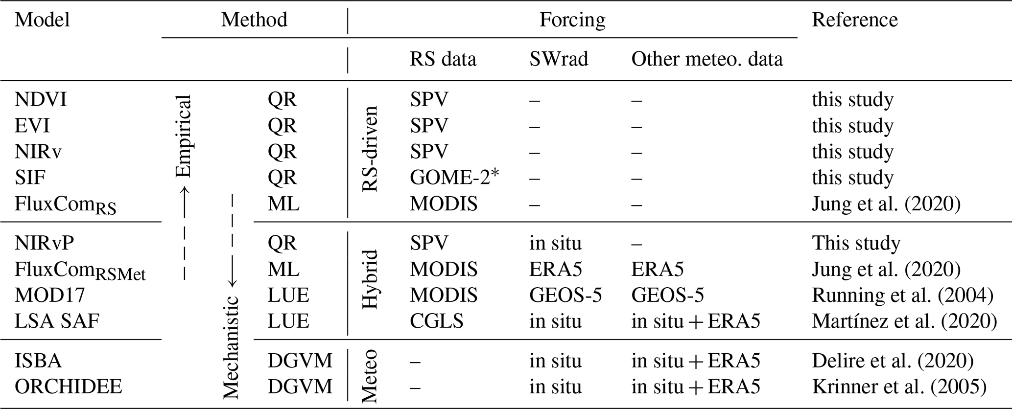
^∗ The SIF data from GOME-2 were the downscaled product from Duveiller et al. (2020), using NIRv, NDWI and LST from MODIS.

Additionally, the canopy structure-related near-infrared reflectance of vegetation multiplied by incoming sunlight (NIRvP) was included (Dechant et al., 2022). It was calculated as follows:

$$\begin{array}{}\text{(4)}& \mathrm{NIRvP}=\mathrm{NIRv}\cdot \mathrm{PAR},\end{array}$$

where PAR is the daily mean photosynthetically active radiation, calculated as a constant fraction (0.45) of the in situ incoming short-wave radiation observations (Howell et al., 1983). For remotely sensed SIF data, we relied on the downscaled GOME-2 SIF product by Duveiller et al. (2020) (8 d interval, 0.05^∘ resolution), given the coarse spatial resolution of the GOME-2 SIF product (> 40 km), sparse global coverage (only a dozen of GOME-2 observations for all tower locations were available per year) and the limited available time series of TROPOMI (starting in May 2018). The downscaling procedure involves a LUE methodology, involving NIRv, normalized difference water index (NDWI; Gao, 1996) and land surface temperature (LST) data from MODIS. Duveiller et al. (2020) demonstrated that this product has a high spatio-temporal agreement with TROPOMI SIF observations, so the impact of the artefacts due to the downscaling procedure are assumed to be limited.

2.4 GPP models

A range of models to estimate GPP was selected, representing RS-driven, meteo-driven and hybrid approaches. An overview is given in Table 2.

RS-based regression models

The simplest models considered were the linear regressions based on remotely sensed proxies of GPP. A robust linear regression model of the RS data versus the daily GPP was constructed using quantile regression (Koenker and Hallock, 2001). The complete dataset was used to obtain a model for each proxy. The use of daily or 16 d average GPP did not have a strong impact on the results. Only NIRvP, which used in situ incoming short-wave radiation observations, had a significantly steeper slope using the daily resolution GPP (see Fig. S1).

Note that the training data used here were also used in the evaluation of the model performance. Furthermore, most models in this study were directly or indirectly trained with data from eddy covariance towers (FluxCom (Jung et al., 2020), ORCHIDEE (Friend et al., 2007), etc.). Consequently, it was not possible to ensure an independent validation of the models. To minimize the impact on the study results, the evaluation was largely based on metrics that are not impacted by the slope of the linear regression (correlation and phenology analysis; see further below). Absolute errors and bias of the models were not evaluated in this study, as these indices are significantly affected by the overlap between training and evaluation data, (but they are shown in Fig. S3 for completeness). Additionally, the robustness of the regression was verified by performing the regression 20 times using a random subset of 50 % of the tower sites (Fig. S1). The regression for NDVI had the largest uncertainty, where the coefficient of variation of the slope was 9 %. For the other proxies, this was around 4 %–5 %. With this result, the quantile regression was found to be robust and independent of the training data sub-selection. The impact of the shared data in the training and evaluation phase on the results is thus assumed to be limited.

Machine learning models

The FluxCom dataset consists of up-scaled FLUXNET observations, using machine learning, remote sensing data and meteorological data (Jung et al., 2020). In this study, we considered the FluxCom_RS GPP product (0.0833^∘ grid, 8 d resolution), which relies on MODIS observations and the FluxCom_RSMet GPP product (0.5^∘ grid, daily resolution), which incorporates supplementary ERA5 meteorological data. Notably, a basic soil water balance model is used to derive the water availability index from the meteorological data and ingest it in the FluxCom_RSMet machine learning algorithm (Tramontana et al., 2016). For each tower location, the closest pixel was extracted from the database.

Light-use efficiency models

As opposed to the pure RS data-driven methods described above, semi-mechanistic models have been developed, which incorporate meteorological forcings to estimate GPP. A widely applied method, thanks to its compatibility with remote sensing observations, is the LUE model (Monteith, 1972). The core of this method is given in Eq. (5), where the plant productivity depends on the absorbed photosynthetic active radiation (APAR) and a light-use efficiency factor (ϵ).

$$\begin{array}{}\text{(5)}& \mathrm{GPP}=\mathit{ϵ}\mathrm{APAR}\end{array}$$

This approach forms the basis of the MODIS MOD17 GPP product (Running et al., 2004) and the LSA SAF GPP product (Martínez et al., 2020).

The algorithm behind MOD17 is a fairly simplistic formulation, where ϵ is linearly dependent on air temperature and vapour pressure deficit. Atmospheric forcings for this product are taken from the GMAO/NASA daily global meteorological reanalysis dataset, generated by GEOS-5 (Goddard Earth Observing System-5). Soil moisture is not considered in the MOD17 model (Running et al., 2004). Conversely, in the LSA SAF model ϵ depends on the ratio between the actual and potential evapotranspiration. Consequently, the impact of soil moisture is indirectly considered.

For MOD17, the closest pixel was extracted for each tower site (MOD17 GPP is available at 1 km resolution with 8 d interval). The LSA SAF GPP in this study was produced by executing the model for each site (as no global coverage or long time series were operationally available in the LSA SAF GPP product). The inputs for this model were leaf area index (LAI) and the fraction of absorbed photosynthetic active radiation (FAPAR) from the Copernicus Global Land Service and ERA5 plus in situ meteorological forcings (see De Pue et al., 2022 for more details on the modelling approach).

Dynamic global vegetation models

DGVMs apply a largely mechanistic methodology to estimate GPP, and its temporal variability is driven exclusively by meteorological forcings. Here, ISBA (Delire et al., 2020) and ORCHIDEE (Krinner et al., 2005) were considered. ISBA is the component within Surfex v8.1 (SURFace EXternalisée), dedicated to the modelling of energy, water, and carbon exchanges between the soil–vegetation–snow continuum and the atmosphere. The numerous processes involved in these exchanges (soil moisture dynamics, evapotranspiration, stomatal closure, canopy growth, canopy radiation transfer, etc.) are fully coupled. Similarly, ORCHIDEE is a well-established model for the simulation of vegetation in the context of earth system models. The version used here was the one that was prepared for the sixth phase of the Coupled Model Intercomparison Project (CMIP6). Both DGVMs share a similar architecture but rely on different formulations for the same processes (e.g. photosynthesis following Goudriaan et al., 1985, and Jacobs et al., 1996, in ISBA versus Farquhar et al., 1980, and Collatz et al., 1992, in ORCHIDEE) and differ in parameterization.

The models were configured to run with identical atmospheric forcing (constructed from ERA5 and in situ meteorological observations), identical land cover and prognostic vegetation growth. These models were run offline and were not coupled to an atmospheric model. For more details on the DGVM configuration and an in-depth evaluation of these models, see De Pue et al. (2022).

2.5 Analysis

To evaluate the performance of the models to capture the temporal variability, the time series in the dataset were decomposed in two ways: (1) by separating the inter-site variability, seasonal variability, and variability of seasonal anomalies and (2) by separating daily, weekly, monthly, seasonal, and interannual components with singular spectral analysis (SSA).

The performance at these timescales was evaluated by comparing the simulated variability (quantified by the standard deviation, σ) in observations and simulations and by computing the Pearson correlation (r). Additionally, the covariance (cov) between GPP and its driver variables was used to assess the sensitivity of GPP to these variables. It was evaluated whether the models reproduce the observed patterns.

Finally, the accuracy of the simulated carbon phenology was evaluated by comparing the timing of the simulated seasonal GPP cycle with observations. Details on the methodology are given below.

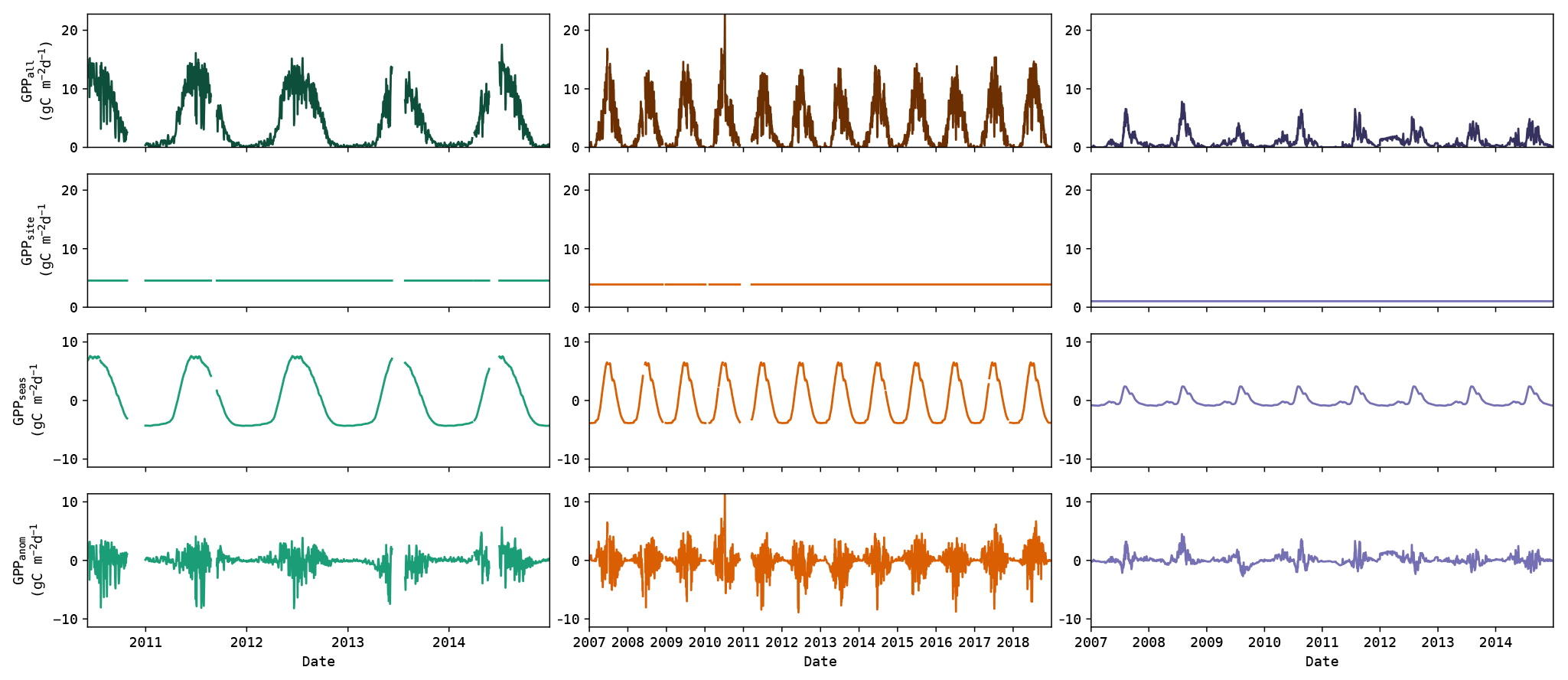
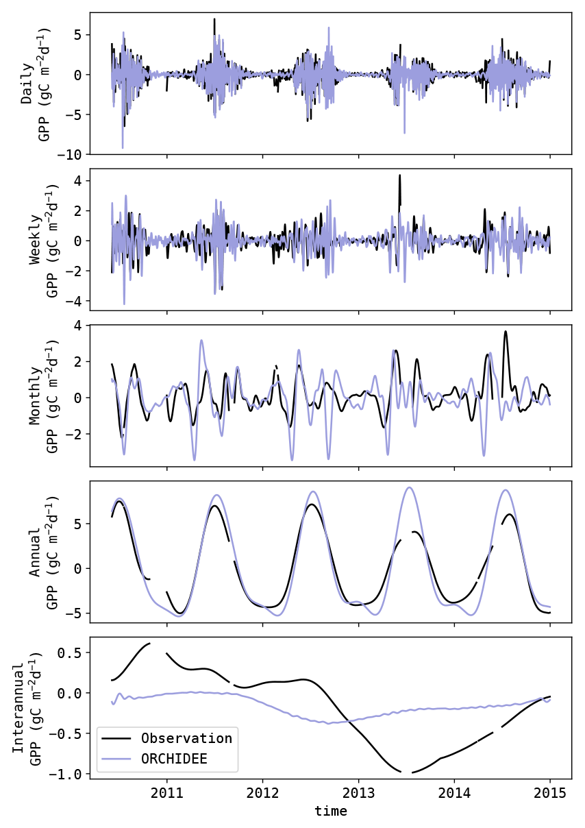
Figure 1 Illustration of the GPP data (top row) decomposition into inter-site (i.e. spatial) component (second row), seasonal component (third row) and the component associated with the anomalies (bottom row). This example shows the observed GPP from DE-Spw, RU-Fyo and US-SRM (left to right, respectively).

Inter-site, seasonal and anomaly components

The variability of the simulated and observed GPP was decomposed into the inter-site (i.e. spatial) component, seasonal component and the component associated with the anomalies. If we concatenate the GPP time series from all sites into one array, we can decompose it as follows:

$$\begin{array}{}\text{(6)}& X_{\text{all}}=X_{\text{site}}+X_{\text{seas}}+X_{\text{anom}},\end{array}$$

where X_all is the full dataset, X_site contains the mean GPP of each site, X_seas contains the mean seasonal cycle of each site (after subtracting the mean of the site) and X_anom contains the resulting anomalies. An illustration of this decomposition is given in Fig. 1. The mean seasonal cycle was obtained by subtracting the time series mean and computing the smoothed (20 d moving average) mean annual cycle. The accuracy of the models to capture each of these components was evaluated using the metrics given further below.

Singular spectrum analysis

To assess the spectral nature of the modelled GPP anomalies, the observed and modelled signals were decomposed in five classes (daily, weekly, monthly, annual and interannual) using singular spectrum analysis (SSA, also referred to as singular system analysis). SSA is a method which allows one to decompose a signal into sub-signals with specific spectral properties (Elsner and Tsonis, 1996; Golyandina et al., 2001). The approach used here was similar to the one proposed by Mahecha et al. (2007). The procedure can be summarized in two steps: the signal decomposition and the reconstruction of the sub-signals. In the signal decomposition step, lagged windows of the original signal were stacked. This array was subsequently decomposed into its underlying orthogonal features by a principal component analysis (PCA). Resulting was a decomposition of the original series in elementary sub-signals, usually characterized by a simple oscillating feature.

Next, these elementary sub-signals were binned according to their spectral properties to reconstruct sub-signals with uniform spectral properties. In this study, similar bins as in the study by Mahecha et al. (2010) were used (see Table 3).

Table 3 Classification of the temporal scales in the SSA.

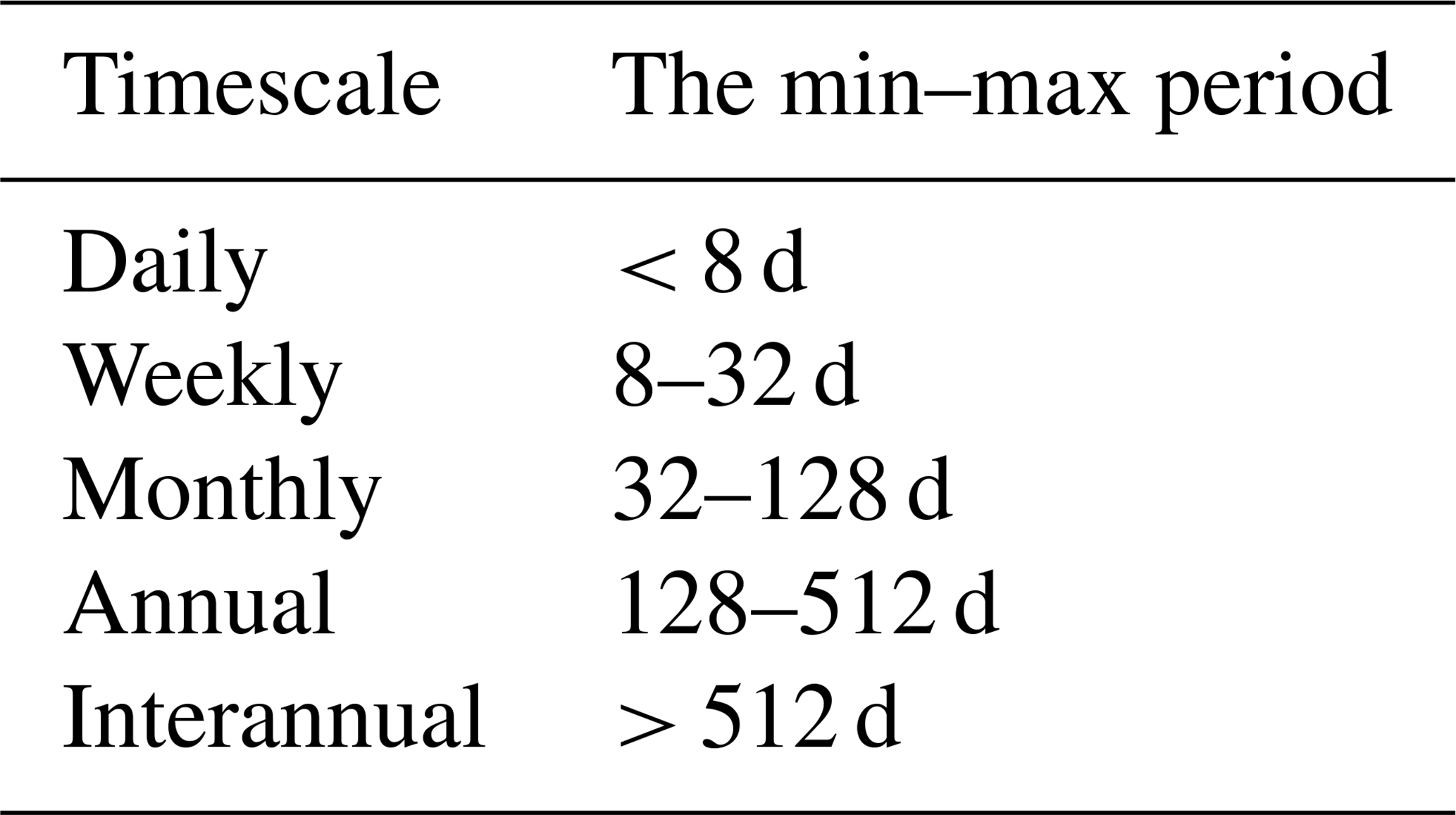
As discussed by Mahecha et al. (2010), some elementary sub-signals might contain features with mixed spectral properties. To avoid this, Mahecha et al. (2010) proposed a double pass procedure, where the SSA is applied again on the reconstructed sub-signals. However, this procedure yielded limited improvements in this study. Instead, it was found to be beneficial to attribute a higher weight to the high-frequency bins compared to the low-frequency bins. This was achieved using weights proportional to the lower-frequency limit of each bin. An example of the analysis is shown in Fig. 2.

Figure 2 SSA decomposition of the observed GPP in DE-Spw and the simulation by ORCHIDEE.

The benefit of SSA compared to other spectral disaggregating methods (e.g. the Fourier transformation) is that it is less sensitive to gaps in the dataset and that it can handle datasets with a lower sampling frequency (e.g. the NDVI time series with 8 d resolution). Consequently, datasets with lower sampling frequency have no signal at the daily timescale. The SSA was applied to the observed and simulated GPP, allowing evaluation at each timescale. The evaluation was performed using the metrics given below.

Performance metrics

The daily GPP estimations from the various models were compared to the observed GPP at the eddy covariance stations (Table 1). The variability of the (decomposed) time series was quantified using the standard deviation of the data (σ). The relative variance (rel.σ²) of a time series component was calculated as

$$\begin{array}{}\text{(7)}& \text{rel.}{\mathit{\sigma }}^{\mathrm{2}}={\displaystyle \frac{{\mathit{\sigma }}_{\text{comp}}^{\mathrm{2}}}{{\mathit{\sigma }}_{\text{all}}^{\mathrm{2}}}},\end{array}$$

where σ_comp and σ_all are the standard deviations (σ) of the component and the full dataset, respectively. This calculation assumes all components to be independent (as the covariance is ignored). It was verified that the covariance of the components is negligible compared to the variance. Detailed results are given in Tables S8 and S9.

Furthermore, the performance of the models was quantified using the Pearson correlation r:

$$\begin{array}{}\text{(8)}& r={\displaystyle \frac{{\sum }^{n_{\mathrm{o}}}(y^{\ast }-\stackrel{\mathrm{‾}}{y^{\ast }})(y^{\mathrm{o}}-\stackrel{\mathrm{‾}}{y^{\mathrm{o}}})}{\sqrt{{\sum }^{n_{\mathrm{o}}}(y^{\ast }-\stackrel{\mathrm{‾}}{y^{\ast }}{)}^{\mathrm{2}}{\sum }^{n_{\mathrm{o}}}(y^{\mathrm{o}}-\stackrel{\mathrm{‾}}{y^{\mathrm{o}}}{)}^{\mathrm{2}}}}},\end{array}$$

where y^∗ and y^o are the predicted and observed values, respectively; $\stackrel{\mathrm{‾}}{y}$ represents the mean of y; and n_o represents the number of observations. Significant differences between the models were evaluated with the Wilcoxon signed-rank test.

Note that MOD17 or FluxCom_RS are 8 d integrated GPP products, yet they are treated here as daily instantaneous products, analogous to the other RS-based GPP products. Consequently, it can be expected that these GPP products will be less capable of estimating the high-frequency anomalies.

Driver variables

Short-wave incoming radiation (SWrad; tower observation), air temperature at 2 m (TA; tower observation), vapour pressure deficit at 2 m (VPD; tower observation) and surface soil moisture (SWC; ERA5) were selected as key hydrometeorological drivers for GPP. Their impact at daily to interannual timescales was assessed by decomposing each time series using SSA and calculating the covariance (cov) with GPP at each timescale. This was computed as

$$\begin{array}{}\text{(9)}& \text{cov}(x,y)={\displaystyle \frac{\mathrm{1}}{n_{\mathrm{o}}}}\sum _{i=\mathrm{1}}^{n_{\mathrm{o}}}(x_i-\stackrel{\mathrm{‾}}{x})(y_i-\stackrel{\mathrm{‾}}{y}),\end{array}$$

where x and y represent two variables (e.g. GPP and SWrad). This analysis was performed for each site separately. The similarity between the observed and simulated covariances was evaluated by comparing the median covariance across all sites and by computing the root mean square error (RMSE) between both. RMSE is computed as

$$\begin{array}{}\text{(10)}& \mathrm{RMSE}=\sqrt{{\displaystyle \frac{{\sum }^{n_{\mathrm{o}}}(y^{\ast }-y^{\mathrm{o}}{)}^{\mathrm{2}}}{n_{\mathrm{o}}}}},\end{array}$$

where y^∗ and y^o are the predicted and observed values (covariances in this case), respectively. SWrad, TA and VPD were collected from the tower meteorological observations. Given that no standardized soil moisture observations were available at each site, SWC was taken from ERA5 (using the 0–7 cm layer) for each location.

As these drivers are not mutually independent, their covariance was evaluated for each HCB and is given in Fig. S4. A positive covariance was found between SWrad, TA and VDP in most sites, and a negative covariance of these variables was found with SWC. The covariances were the strongest at the seasonal timescale. Most HCB classes showed similar behaviour, with some exceptions in the Tropic and Trans_W biomes.

Carbon phenology

The (carbon) phenology in the time series was quantified by the timing of the start, maximum and end of the seasonal GPP cycle (SOS, MOS and EOS, respectively). This was achieved by applying a smoothing operation (20 d rolling mean), followed by a threshold procedure (Maleki et al., 2020; De Pue et al., 2022). In this procedure, the minima and maxima were used to delineate the growing and senescent phase of the season. MOS was defined as the date when the maximum of the season is reached, SOS and EOS were defined at the dates where the growing or senescent phase cross the threshold value T. And T was calculated for each growing or senescent phase as $T=P_{\mathrm{5}}+\mathrm{0.2}(P_{\mathrm{95}}-P_{\mathrm{5}})$, where P₅ and P₉₅ are the 5th and 95th percentiles. If the seasonal cycle was not pronounced enough ($(P_{\mathrm{5}}-P_{\mathrm{95}})/P_{\mathrm{50}}<\mathrm{0.2}$), the detected phenology was considered unreliable and omitted. The bias and accuracy of the phenology were evaluated by calculating the mean error (ME) and root mean square error (RMSE).

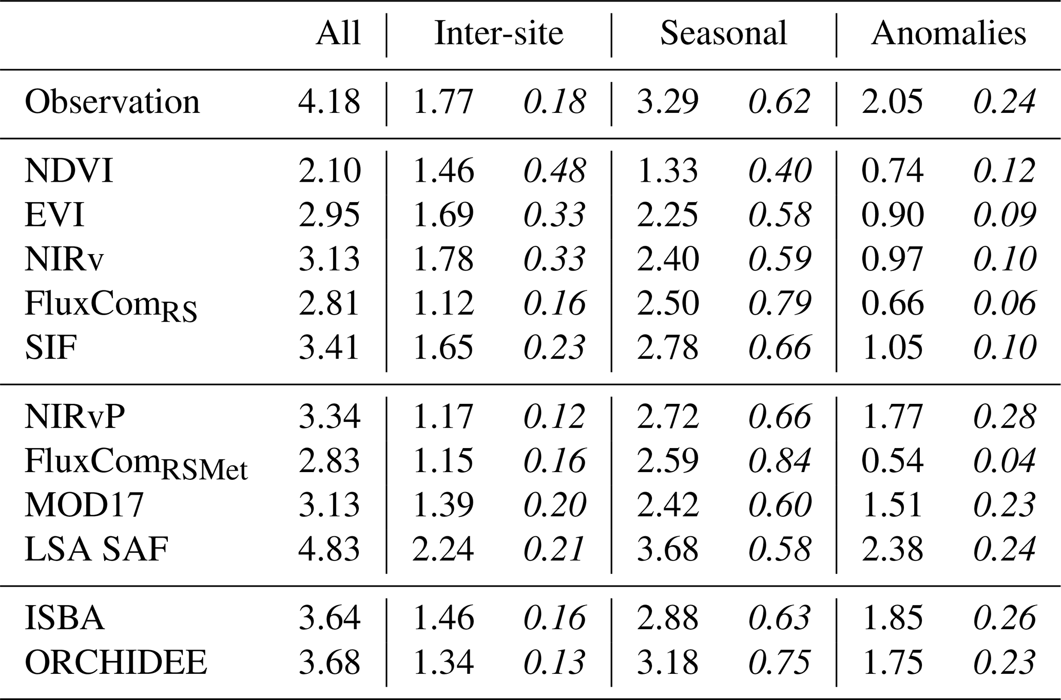
Table 4 Standard deviation of the observed and simulated GPP ($\mathrm{g}\mathrm{C}{\mathrm{m}}^{-\mathrm{2}}{\mathrm{d}}^{-\mathrm{1}}$), decomposed into the inter-site, seasonal and anomaly (obtained after subtracting the spatial and seasonal component) components, and the fraction of the total variance (italics). This analysis done after grouping all sites together.

3 Results

3.1 Inter-site and seasonal variability

A comparison of the variability of GPP in observations and simulations is given in Table 4. The overall observed variability of σ = 4.18 $\mathrm{g}\mathrm{C}{\mathrm{m}}^{-\mathrm{2}}{\mathrm{d}}^{-\mathrm{1}}$ was underestimated in all models, except LSA SAF. After decomposing the observed GPP dataset, the inter-site variance represented 18 % of the total variance, the seasonal cycles represented 62 % and the anomalies represented 24 % (the sum of these fractions is larger than 100 % due to covariances; see Tables S8 and S9). This partitioning was not well represented in the NDVI, EVI or NIRv time series, where a large fraction of the variance (> 30 %) was attributed to the inter-site component and a very small fraction (< 12 %) to the anomalies. In the NDVI observations, the inter-site variance was even larger than the seasonal variance. In SIF, the contribution of the spatial and seasonal components was reasonably accurate, but the relative variance of the anomalies was too low (10 %). The relative variance of the seasonal pattern was strongly overestimated in the FluxCom products (∼ 80 %), whereas the contribution of the anomalies was the lowest of all datasets (∼ 5 %). The closest match with the observed variance partitioning was found in NIRvP, MOD17, LSA SAF and the DGVMs. To ensure that these results were not affected by the temporal resolution of the time series, the same analysis was performed after downsampling to a 10 d interval. This did not result in substantial changes in the variability or its partitioning (Table S6).

Depending on the land cover type, the variability and its partitioning between different components varied (Table 5). As expected, limited seasonal variability was observed in the EBF-Tropic sites (σ_season = 0.68 $\mathrm{g}\mathrm{C}{\mathrm{m}}^{-\mathrm{2}}{\mathrm{d}}^{-\mathrm{1}}$) compared to DBF-MidL_T sites (σ_season = 5.11 $\mathrm{g}\mathrm{C}{\mathrm{m}}^{-\mathrm{2}}{\mathrm{d}}^{-\mathrm{1}}$). Still, the variability of the anomalies of the tropical sites was comparable to that in other sites (σ_anom≈ 2.00 $\mathrm{g}\mathrm{C}{\mathrm{m}}^{-\mathrm{2}}{\mathrm{d}}^{-\mathrm{1}}$). The CRO-MidL_T sites had the largest variability in the anomalies (σ_anom = 3.43 $\mathrm{g}\mathrm{C}{\mathrm{m}}^{-\mathrm{2}}{\mathrm{d}}^{-\mathrm{1}}$).

Table 5 Median standard deviation of the observed GPP per land cover class ($\mathrm{g}\mathrm{C}{\mathrm{m}}^{-\mathrm{2}}{\mathrm{d}}^{-\mathrm{1}}$), decomposed into the seasonal component and its anomalies. The fraction of the total variability is given in italics.

The Taylor diagram of the modelled GPP and its seasonal anomalies is shown in Fig. 3. In terms of correlation, the DGVMs, LSA SAF and the FluxCom products achieved a distinctly better performance (r>0.83, median for all sites) compared to the linear-regression-based models (and MOD17). The NDVI-based model had the weakest correlation with observations (r=0.57, median for all sites). The correlation of the simulated GPP was substantially reduced after subtracting the mean seasonal cycle. For NDVI, EVI, NIRv and SIF, r_anom was smaller than 0.2 (median for all sites). LSA SAF and ISBA were the only models with r_anom>0.5 (median for all sites). The performance of FluxCom to estimate the anomalies was similar to the NDVI-, EVI- and NIRv-based models. Though FluxCom_RSMet achieved r_anom=0.43 (median for all sites), the variability of the anomalies was strongly underestimated.

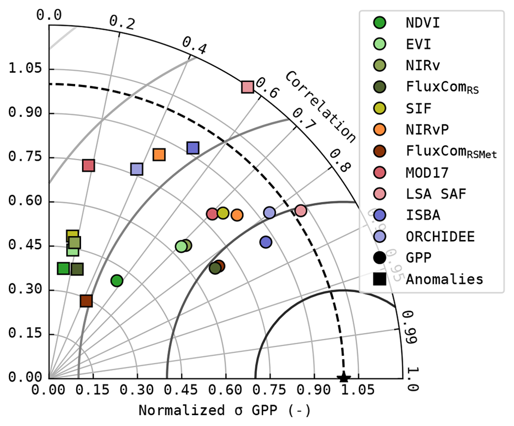
Figure 3 Taylor diagram of the simulated GPP (circles) and its seasonal anomalies (squares); median of the metrics at all sites.

A notable difference emerged in the anomalies simulated with NIRvP and SIF. While both datasets showed a similar performance in the full GPP time series, SIF performed much poorer than NIRvP in the anomalies.

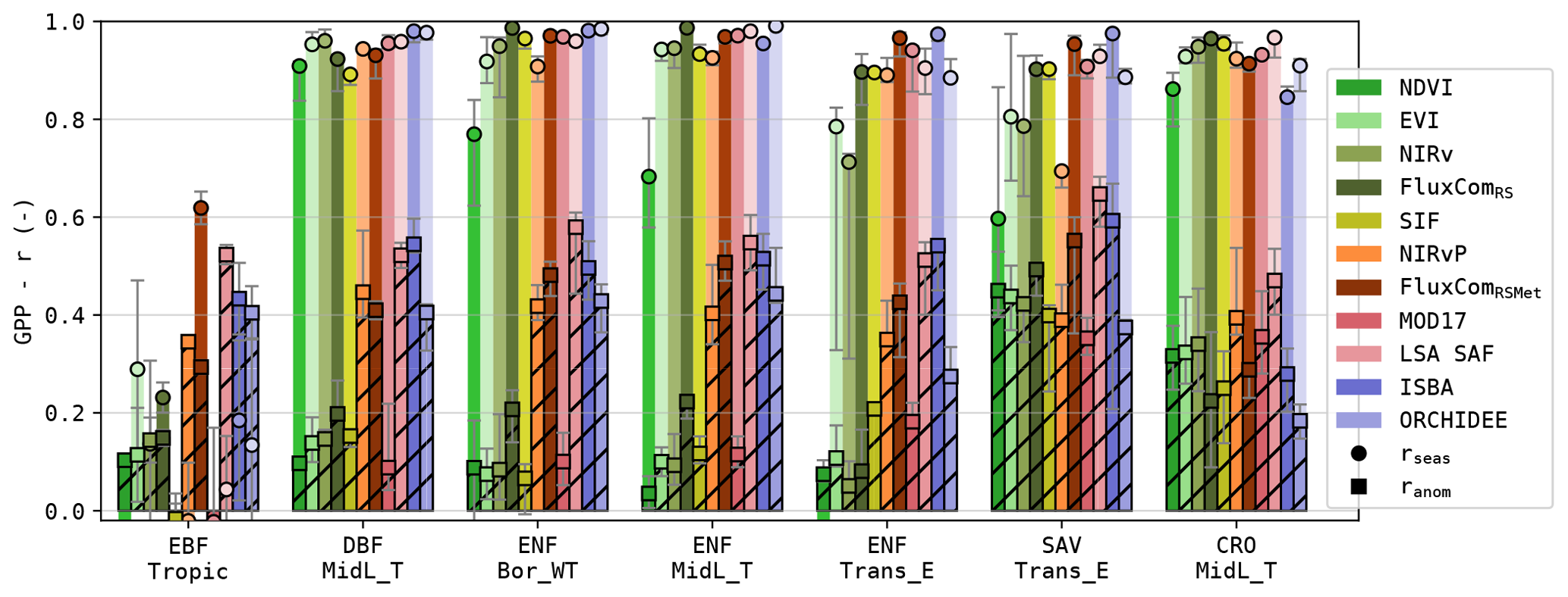
Figure 4 Pearson correlation of the modelled GPP and its anomalies for sites in seven PFT-HCB classes (see Table 1).

The RS-driven models, which relied purely on RS observation of the vegetation state, had a significantly lower σ_anom (Wilcoxon p<0.05) compared to the models that used meteorological forcing. This difference in performance was most pronounced in the forest sites (Fig. 4). In sites dominated by (water-limited) herbaceous vegetation, this was less the case; GPP estimations based on simple greenness sensitive NDVI-, EVI- and NIRv-based models often even outperformed DGVMs.

Table 6 Standard deviation of the observed and simulated GPP ($\mathrm{g}\mathrm{C}{\mathrm{m}}^{-\mathrm{2}}{\mathrm{d}}^{-\mathrm{1}}$), decomposed into the different timescale components using SSA (median values for all test sites). The fraction of the total variability is given in italics.

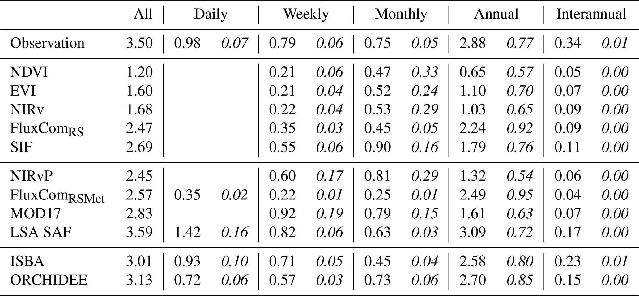
3.2 Timescale disaggregation

The variability of the time series after SSA decomposition is given in Table 6. In agreement with the variability of the seasonal GPP and its anomalies, the largest variability was explained by the annual timescale (77 %, median for all sites). At daily, weekly and monthly timescales, the relative variance was roughly 10-fold smaller. The least variability was found for the interannual timescale (1 %, median for all sites). More detailed results per land cover type are given in Table S6. Most land covers followed the same pattern, with the exception of the EBF-Tropic sites, where seasonal variance was smaller than the variance at daily, weekly, monthly or even annual timescales.

The RS-driven models underestimated the variance at all timescales, especially at the annual scale. Furthermore, very limited variability was found at the interannual scale, and the relative variance at monthly scale was overestimated in these models. NDVI was the least suitable proxy to capture this variability, whereas the relative variance partitioning in SIF approximated most closely the observations. Notably, the inclusion of PAR in NIRvP improved the GPP variability but degraded the variance partitioning across timescales.

The FluxCom products contained a too strong annual signal and underestimated variability at other scales. The incorporation of daily meteorological forcing in FluxCom_RSMet added variability at the daily timescale but reduced variability at weekly and monthly timescales. The annual variability was approximated relatively well, but the variability at shorter timescales was roughly 3-fold too small.

The variability across all timescales was best represented by the meteo-driven DGVMs (Table 6). There were minor differences between ORCHIDEE and ISBA, as the variance at daily and weekly timescales was slightly more accurate in ISBA, and the variance at monthly and annual timescales was more accurate in ORCHIDEE. This trend was confirmed in most land covers (see Table S6). LSA SAF also estimated the variability reasonably accurately but overestimated the daily variability.

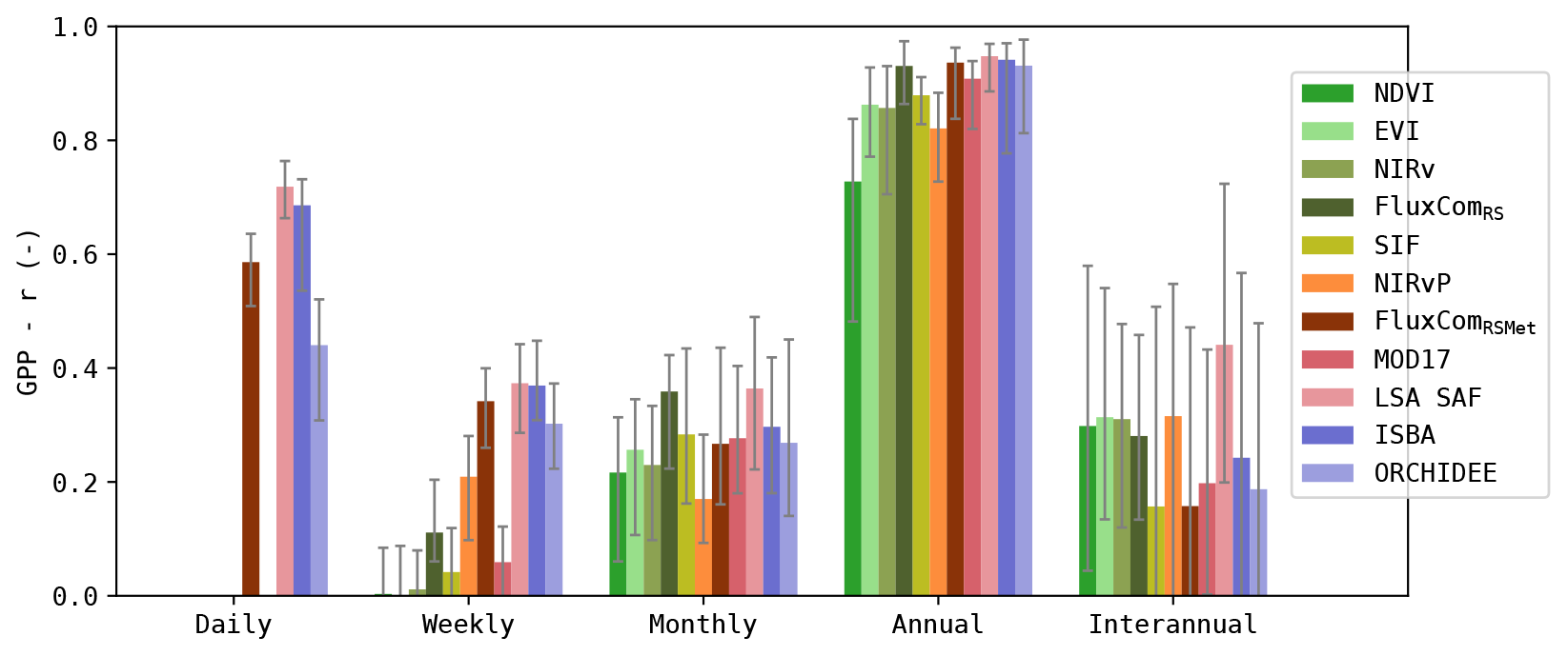
Figure 5 Pearson r across timescales after SSA decomposition; median score for all sites. Error bars indicate the 25–75 quantiles.

The correlation of the simulations at these timescales is given in Fig. 5. Note that the strength of the signal at interannual scale was relatively low (in observed and simulated GPP). Evaluating the correlation of this component should thus be done with caution, as the SSA itself can induce errors of comparable magnitude (Mahecha et al., 2010). It is shown here but not discussed in detail.

Most models had a good correlation with GPP at the annual timescale (r>0.80, median for all sites), except the NDVI-based model. At monthly the timescale, the correlation dropped to r≈0.25 for all models (median for all sites). At weekly timescale, the models that relied solely on remote sensing observations were very poorly correlated to the observed GPP. Compared to these models, the models that included meteorological data achieved a significantly higher correlation (Wilcoxon p<0.05). At daily scale, r increased again. LSA SAF and ISBA achieved r>0.65 (median for all sites) at this spectral range.

Figure 6 Pearson r in DBF, ENF, SAV and CRO across timescales.

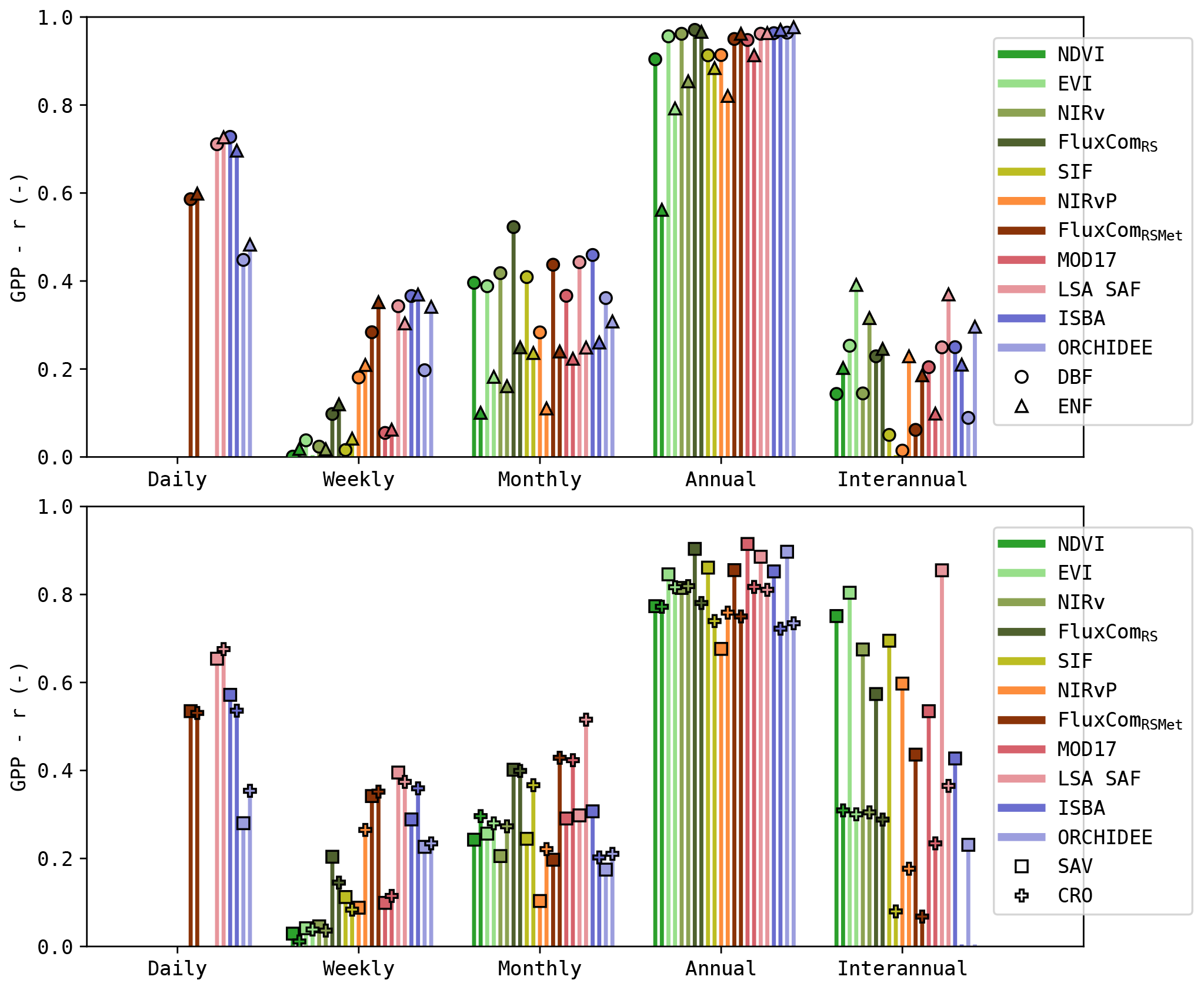
Separating the results by PFT (Fig. 6) shows that the correlation at monthly and seasonal timescales was generally larger for DBF sites compared to ENF sites. At seasonal scale, this was most pronounced for the greenness-sensitive VI proxies (NDVI, EVI and NIRv).

Dryland sites, such as the SAV sites, generally showed a higher correlation at the interannual scale for the RS-driven models. Not all models manage to capture these interannual patterns. For example, ORCHIDEE obtained only a very low correlation at this scale. Regardless, the interannual scale had only a minor contribution to the total variability.

In the CRO sites, the RS-driven models had a significantly lower r at weekly timescale compared to the DGVMs (Wilcoxon p<0.05, with the exception of NIRv vs. ORCHIDEE and MOD17 vs. ORCHIDEE). However, at the monthly timescale, the RS-driven models had a higher r than the DGVMs (significantly for SIF, FluxCom_RS and MOD17), and at the annual scale this trend persisted (significantly for EVI, NIRv, FluxCom_RSMet and MOD17).

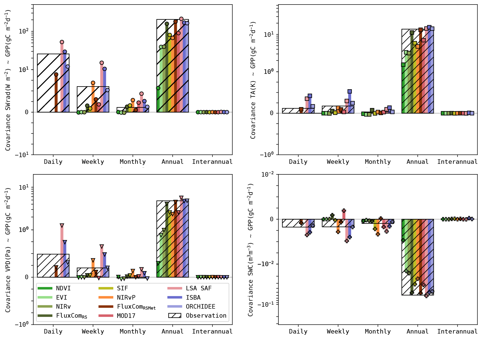
Figure 7 Covariance (median for all sites) of the simulated GPP and its drivers (SWrad, TA, VPD and SWC). Covariance based on observations is shown with the bars with hatching. The coloured bar plots indicate the covariance in the simulations. Note that the covariance is shown using a symmetric log scale.

3.3 Drivers of GPP

Given the different performances across timescales, the covariance between the GPP and its key drivers (SWrad, TA, VPD and SWC) was evaluated. The observed and simulated covariances are shown in Fig. 7. These are the median covariances for all sites. The covariance is impacted by the variance of the GPP estimates, as opposed to the Pearson correlation. For completeness, the latter is computed as well and is given in Fig. S5.

In the observations, all drivers had the highest covariance with GPP at the seasonal scale. SWrad and VPD had a stronger covariance at daily scale compared to weekly and monthly timescales, whereas TA had a slightly stronger covariance at weekly timescale. The covariance between SWC and GPP was negative, indicating that GPP was smaller during wet root-zone soil moisture anomalies (and higher during dry anomalies). This was largely attributed to the negative covariance between SWC and the other drivers, as wet conditions are associated with periods of rain and cloudy weather (Fig. S4). The covariance between GPP and SWC was similar at daily, weekly and monthly timescales. For all drivers and GPP, the interannual signal was very weak, resulting in a negligibly small covariance.

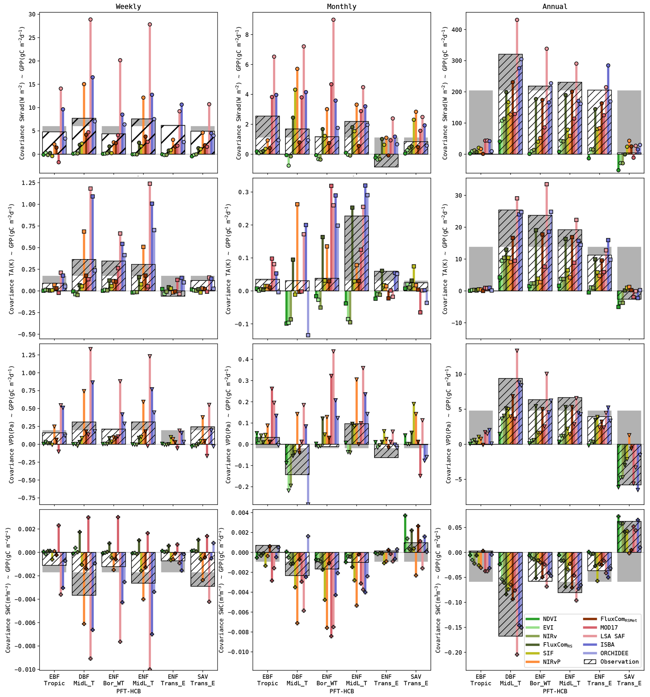
Figure 8 Covariance of the simulated GPP and its drivers at weekly, monthly and seasonal timescales. Covariance based on observations are in the bars with hatching, and grey bars highlight the deviation for a land cover from the overall average. The coloured bar plots indicate the covariance in the simulations.

Substantial differences in the observed correlations were found between different biomes, as highlighted in the plots of the weekly, monthly and annual covariance (Fig. 8). For example, the covariance between SWrad and GPP at the annual scale was very strong for most biomes, but it was very weak for EBF-Tropic (due to a small variability of the GPP signal at this scale) and SAV-Trans_E sites (due to downregulation of photosynthesis by other constraining factors). Another clear trend was the shift in covariance between SWC and GPP from negative in biomes where water is not a constraining factor (e.g. DBF-MidL_T) to water-limited biomes (e.g. SAV-Trans_E).

The accuracy of the models to reproduce these patterns was quantified by RMSE (see Tables S10 and S11 for detailed results). The RS-driven models generally had a very low sensitivity to all drivers at weekly and monthly timescales. The covariances at annual scale were underestimated as well. This can be attributed partly to the lower variance of the RS-driven GPP estimates at annual scale, but the Pearson r also indicated a too low sensitivity (Fig. S6). Conversely, the sensitivity of the meteo-driven models was generally more accurate. Some oversensitivity to the meteorological drivers was found in ISBA, whereas ORCHIDEE was generally among the most accurate models. The covariance with soil moisture was more accurate in ISBA than ORCHIDEE (e.g. RMSE at weekly, monthly and annual scales 10 %–30 % more accurate)

The performance of the hybrid models was highly variable. LSA SAF was generally too sensitive to meteorological drivers, whereas MOD17 (also a LUE model) was too insensitive to all drivers (though more sensitive than the RS-driven models). The covariance of GPP with its drivers was generally most accurate in the FluxCom products. Their largest shortcoming was a too low sensitivity to SWrad at daily and weekly timescales.

The dynamics in temperate DBF forest sites were reproduced fairy well by most models. The strong annual covariances were represented well by all models. Even the RS-driven models had a relatively high covariance at this scale. At annual scale, the DGVMs and LSA SAF were most accurate in this biome (RMSE 3- to 4-fold lower than RS-driven models). In contrast, the high annual covariance was not represented well by the NDVI-, EVI- and NIRv-based models in the ENF sites. The covariance between GPP and the drivers at annual scale was generally too weak. FluxCom and the DGVMs were more accurate (RMSE 4- to 5-fold lower than in VI-based models).

VPD and SWC were strong drivers for annual variability in the savanna sites. This was reproduced accurately by the RS-driven models and ISBA. NIRvP, FluxCom_RSMet and ORCHIDEE did not capture the annual covariance with VPD and SWC (RMSE for SWC and VPD 2- to 3-fold higher than ISBA, i.e. the most accurate model).

In the EBF-Tropic biome, all models had a too strong relation with the drivers at annual scale. A resemblance with the observed annual relations was found only in the FluxCom_RSMet product. It was the only model with an accurate positive GPP-SWC annual covariance for the EBF-Tropic sites.

The results for the FluxCom products highlight the importance of incorporating meteorological forcings in the GPP product. FluxCom_RSMet was superior to FluxCom_RS in the reproduction of GPP at different timescales. The coarser spatial resolution of FluxCom_RSMet did not have a negative impact on the performance in this study.

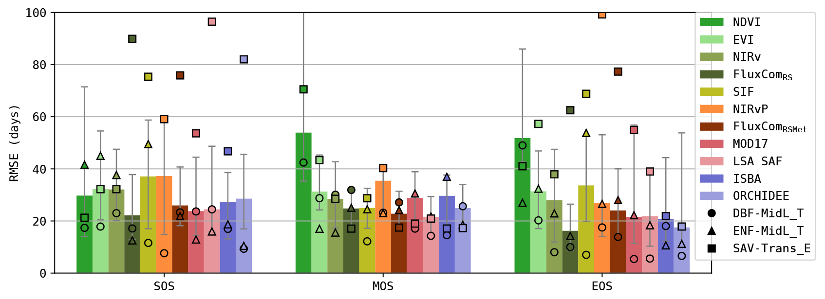
Figure 9 RMSE (per site) in the timing of the start, max and end of the seasonal GPP cycle (SOS, MOS and EOS). Bars show overall results (median for all sites); markers show separate results for three PFT-HCB classes.

This analysis gives a coarse estimate of the (linear) sensitivity of the simulated GPP to the drivers impacting GPP. Note that many effects were not accounted for, including compound effects, legacy effects or the impact of other constraining variables (e.g. LAI in the DGVMs).

3.4 Phenology

The accuracy of the simulated timing of the seasonal GPP cycle (start, max and end of season) is plotted in Fig. 9 (RMSE scores are calculated for every site individually). Generally, the simulations of SOS and EOS were generally less accurate in the RS-driven models (RMSE SOS ≈ 30–38 d, EOS ≈ 25–50 d; except FluxCom_RS) compared to the meteo-driven models (RMSE SOS ≈ 24–28 d, EOS ≈ 17–21 d). The phenology in the NDVI-based model was the least accurate, which was largely attributed to a bias in the timing, especially in the EOS (≈ 50 d delayed; see Fig. S7). This bias was also observed in EVI and NIRv but was smaller (≈ 10 d delayed). Notably, the most accurate simulations of SOS and EOS were obtained with FluxCom_RS, which purely relied on remote sensing observations.

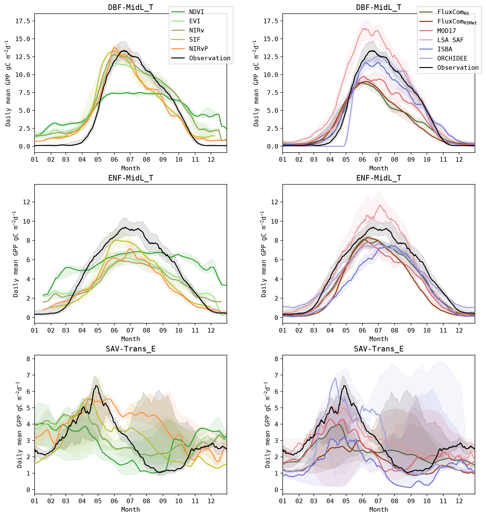
Figure 10 Annual GPP cycle in observations and models for sites in the DBF-MidL_T, ENF-MidL_T and SAV-Trans_E biomes. The lines show the median cycle, and the shaded area shows the 25–75 percentile. Time series of sites located at the Southern Hemisphere were shifted by 6 months to match with the annual cycle of sites in the Northern Hemisphere.

To highlight differences between biomes, the mean annual cycle of DBF-MidL_T, ENF-MidL_T and SAV-Trans_E is plotted in Fig. 10 (the annual cycle of the other biomes can be found in Figs. S8 and S9). The DBF-MidL_T had a very distinct SOS around the fifth month of the year. The interannual variability of the observed GPP cycle was limited compared to other biomes. Most models reproduced the phenology fairly accurately. In the NDVI time series, an evident illustration of the so-called “saturation effect” was observed, as the simulated GPP reached a plateau during mid-summer.

In the ENF-MidL_T biome, the coupling between canopy greenness and GPP was less strong than in DBF-MidL_T. Consequently, the meteo-driven and hybrid models were generally more accurate to simulate the timing of the GPP cycle in this biome (RMSE SOS ≈ 10–18 d, EOS ≈ 10–18 d; see also Fig. 9) than the RS-driven models (RMSE SOS ≈ 35–50 d, EOS ≈ 22–50 d). Also note the delayed MOS in the ISBA simulations for this biome. This was largely associated with the delay in the prognostic LAI seasonal cycle (De Pue et al., 2022).

A strong variability of the annual GPP cycle was observed in the SAV-Trans_E biome (Fig. 10), making it very challenging to capture the timing of the GPP cycle accurately (Fig. 9). However, in these sites, a stronger coupling existed between GPP and the canopy greenness. At the SOS, a distinct difference between the RS-driven models and the meteo-driven models emerged. The RS-driven models were more accurate (RMSE SOS ≈ 20–30 d for NDVI, EVI and NIRv) compared to the DGVMs (RMSE SOS ≈ 46–82 d). In this biome, the inclusion of PAR in NIRvP resulted in a less accurate phenology compared to NIRv. In NIRv, the reduced photosynthesis due to water-limiting conditions in the second half of the growing season was evident, whereas GPP remained high in NIRvP.

4 Discussion

The variability of GPP is largely modulated by the vegetation state (canopy greenness, leaf area index, etc.) and hydrometeorological conditions. As indicated by Stoy et al. (2009), the relation of GPP to these factors shifts across timescales: “Quantifying flux variability at longer timescales requires information on how ecosystems change in response to climatic variability, rather than how they merely respond to climatic variability”. In this study, we investigated how well the impact of these factors is captured in RS-driven, meteo-driven and hybrid models.

4.1 Vegetation state

Depending on the biome, the vegetation state is tightly coupled (e.g. in water-limited herbaceous sites), more loosely coupled (e.g. deciduous broadleaf forests) or completely decoupled (e.g. tropical evergreen broadleaf forests) to GPP (Hu et al., 2022). Vegetation indices, such as NDVI, EVI and NIRv are effective proxies to track the vegetation state via remote sensing. They have proven to be an effective, low-cost proxy for GPP in biomes with an evident coupling between canopy greenness and photosynthesis (Xiao et al., 2019; Huang et al., 2019).

However, an important discrepancy was found between the RS observations and the observed GPP in the spatio-temporal partitioning of their variability. The inter-site variability of NDVI, EVI, NIRv and (to a lesser extent) SIF was substantially higher than that of the GPP observations. Furthermore, the variability of the anomalies in the models was relatively small (see Tab 4). This high inter-site variability indicated that there was a need to use land-cover-dependent relations to estimate GPP from the remotely sensed vegetation proxies. Several studies have confirmed that PFT-specific relations considerably improved the GPP estimates from NDVI (Huang et al., 2019), EVI (Shi et al., 2017; Huang et al., 2019), NIRv (Badgley et al., 2019; Huang et al., 2019) and SIF (Gao et al., 2021). FluxCom_RS also relied on land cover data to estimate GPP from RS observations (Jung et al., 2020) and captured the spatial and seasonal variability more accurately (see Table 4). Results from explorative tests with PFT-specific regression models are shown in Figs. S10 and S11. They indicated that improved results were largely caused by improved spatial correlation. The variability of the seasonal signal and anomalies remained underestimated.

The biome-dependent relation between vegetation greenness and GPP was also evident in the seasonal cycle (Fig. 4) and in the annual timescale (Fig. 6). For DBF and CRO biomes, the coupling between VI and GPP resulted in high correlations at these timescales, whereas the decoupling in other biomes emerged. This was most pronounced in evergreen forest sites (ENF and EBF), and the decoupling increased as the climate was increasingly water-limited (ENF-Bor_WT < ENF-MidL_T < ENF-Trans_E; see Figs. 4 and 8). Opposed to herbaceous sites in the same arid biomes (e.g. SAV-Trans_E), the photosynthesis downregulation in ENF sites was not translated into rapid changes in vegetation greenness.

As often reported, the decoupling of leaf phenology and carbon phenology was also poorly captured in the VI-based models. This was most pronounced in the senescent phase, where photosynthesis halts, due to decrease in SWrad and TA, before canopy greenness drops (Kong et al., 2020; Wang et al., 2020).

All VIs were insensitive to the decoupling of canopy greenness and photosynthesis at seasonal timescale, but NDVI performed significantly worse than EVI and NIRv in this respect. Saturation in dense canopies, background effects and atmospheric influences (Huete et al., 2002; Olofsson et al., 2008) likely explain the underestimated variability of the seasonal cycle in NDVI time series, especially in forest biomes (illustrated in Fig. 10). Between EVI and NIRv, no substantial differences in performance were found.

SIF is a more direct proxy for photosynthesis and is therefore expected to capture the decoupling between vegetation greenness and GPP more accurately than VIs (Duveiller et al., 2020; Pickering et al., 2022). However, SIF did not perform significantly better than EVI or NIRv at the annual timescale (Figs. 5 and 6). Exceptions were the arid biomes, ENF_Trans-E and SAV_Trans-E, where SIF outperformed EVI and NIRv. It remains unclear in what measure the downscaling processing is responsible for the moderate SIF scores. Future missions with high-resolution SIF, such as European Spatial Agency's Earth Explorer – FLEX (FLuorescence EXplorer, due to be launched in 2025), will provide further insights (Duveiller et al., 2020).

The results with the VI-based models seemed to indicate that the remotely sensed observations of the vegetation state were insufficient to describe GPP in evergreen vegetation. However, FluxCom_RS relied exclusively on these observations as predictors and managed to capture GPP patterns in ENF. Furthermore, it produced the most accurate results regarding the GPP phenology. This product illustrated that, in combination with land cover information and non-linear relations, accurate estimates of GPP at the seasonal timescale can be obtained from optical remote sensing (Tramontana et al., 2016).

Conversely, it is very challenging to accurately model the state of the vegetation without RS observations (Fatichi et al., 2019). In a detailed evaluation of the water, energy and carbon modelling in ISBA and ORCHIDEE, it was reported that the leaf phenology in ISBA and ORCHIDEE was delayed compared to observations and that it failed to capture the observed seasonal variability. De Pue et al. (2022) reported that these errors were strongly correlated to errors in GPP. Despite these inaccuracies, the performance of the DGVMs was generally better than the VI-based models. The dominant impact of meteorological forcings and the decoupling of greenness and photosynthesis was captured accurately in the DGVMs.

Next to the complexity of plant physiology and biomass allocation; there can be a substantial impact of management practices (e.g. crop rotations, sowing and harvest in croplands; Osborne et al., 2010). The lack of these practices in the configuration of the DGVMs in this study also resulted in a poorer performance of the monthly and annual-scale GPP in croplands (see Fig. 6). Observations of these practices in remote sensing contribute to a better performance in croplands with RS-driven models. At a global scale, the lack of an adequate description of land management contributes considerably to uncertainties associated with the global carbon cycle in earth system models (Friedlingstein et al., 2022).

In summary, based on the observed vegetation state, a coarse estimate of the annual-scale GPP can be made. However, vegetation indices and linear regressions are insufficient to capture the decoupling of greenness and photosynthesis due to other confounding factors. Information on the hydrometeorological conditions is needed to capture this variability in all biomes, even at the seasonal scale.

4.2 Meteorological conditions

Meteorological conditions are the main drivers of variability of GPP at sub-seasonal scale (Stoy et al., 2009). At daily timescale, patterns were largely dominated by SWrad and VPD (see Fig. 7). The impact of TA was more pronounced at weekly and monthly timescales (though still dominated by SWrad).

The RS-driven models had a very low performance to simulate these sub-seasonal patterns (Fig. 5). They had a temporal resolution of 8–10 d, so the variability at daily timescale was absent. At weekly and monthly timescales, they had nearly no sensitivity to the driver variables (Fig. 7). Consequently, the correlation of the anomalies was very weak in comparison to other models (Fig. 4).

NIRvP was the most simplistic approach to incorporate SWrad (as PAR) as key driver for photosynthesis (Eq. 4). Compared to NIRv (and SIF), NIRvP captured anomalies in GPP more accurately, in particular at the weekly timescale (Figs. 3 and 5).

Alternatively, light-use efficiency models ingest more meteorological variables, such as VPD and TA, in addition to SWrad and vegetation state variables. Consequently, the quality of the simulated GPP strongly depended on the quality of the meteorological forcings. The MOD17 product relied on the coarse GMAO/NASA reanalysis dataset for the meteorological forcing and failed to achieve a better performance than the VI-based models (Fig. 3). The LSA SAF GPP model, here forced by in situ SWrad observations, excelled in the simulation of temporal variability at all timescales and in all domains. Although there were other factors that impact the performance (e.g. the incorporation of soil moisture stress, which was absent in MOD17), the difference in SWrad forcings likely contributed substantially to the difference in performance, given the sensitivity of the models to SWrad and the quality of SWrad in reanalysis products (Anav et al., 2015; Urraca et al., 2018; Zheng et al., 2018).

The incorporation of meteorological forcings in FluxCom_RSMet improved the algorithm's ability to capture the anomalies compared to FluxCom_RS (Fig. 3). This was most evident in forest sites (Fig. 4), though the improvement was restricted to the weekly timescale (Fig. 5). Still, despite the introduction of meteorological variables, the variance of the anomalies remained strongly underestimated (Table 4).

In contrast, the meteo-driven DGVMs represented the variability of GPP accurately across timescales. A significant difference between ISBA and ORCHIDEE was found in the performance at daily timescale (Fig. 5). The superior performance of ISBA at this timescale seemed to be originating from a more accurate sensitivity to SWrad than ORCHIDEE (Fig. 7). Conversely, the sensitivity to atmospheric drivers at weekly and monthly timescales was more accurate in ORCHIDEE, whereas ISBA was generally oversensitive (Figs. 7 and 6). Though the performance of ORCHIDEE to simulate GPP at these longer timescales was not superior (due to other confounding factors, e.g. soil moisture or LAI), ORCHIDEE is likely more accurate in assessing the impact larger meteorological anomalies, such as heat waves, on GPP. Further research addressing the performance of the models under extreme conditions is needed to confirm this.

4.3 Soil moisture

At sub-seasonal scale, the RS-driven models demonstrated a big difference in performance between forest and herbaceous biomes. A substantially better performance was achieved in herbaceous sites (Fig. 4), where the coupling between vegetation greenness and GPP is much tighter than in forest sites Hu et al. (2022). The indirect observation of soil moisture stress in VIs allowed for accurate sub-seasonal-scale modelling of GPP in these strongly water-limited biomes (AghaKouchak et al., 2015). In other biomes, the combination with a drought indicator is required to simulate GPP in such conditions (Maleki et al., 2022).

No downregulation due to soil moisture or temperature stress is considered explicitly in NIRvP. However, changes in light-use efficiency are partly reflected in changes in the canopy structure (Xu et al., 2021). Consequently, NIRvP can yield similar results than SIF, as demonstrated in the work by Dechant et al. (2022). Regardless, in water-limited herbaceous sites (e.g. SAV-Trans_E), the sensitivity to soil moisture stress in NIRv was eliminated in NIRvP, due to a too high sensitivity to SWrad (Fig. 8). An illustration of this lack of soil moisture stress downregulation was evident in the mean annual cycle of NIRvP, where GPP was consistently overestimated during the dry season (Fig. 10). The downregulation was more accurately reflected in the SIF model.

The seasonal GPP patterns in water-limited sites (e.g. ENF-Trans_E or SAV-Trans_E) were generally simulated less accurately (see Fig. 4) in DGVMs, indicating that the soil moisture dynamics or the soil moisture stress response of the vegetation were an important source of errors (Vereecken et al., 2019; Raoult et al., 2021; De Pue et al., 2022). In the arid biomes, differences between ISBA and ORCHIDEE were most evident. The soil moisture dynamics and response to soil moisture stress in ORCHIDEE were demonstrated to be less accurate compared to ISBA in a previous study by De Pue et al. (2022).

4.4 Uncertainties

The in situ observation uncertainty may contribute to the disagreement between models and observations. The eddy covariance observations are associated with site-dependent random errors due to instrumentation, stochastic nature of turbulence and varying footprint (Mauder et al., 2020). Additionally, the typical non-closure of the energy balance might indicate that the observed carbon fluxes suffer from a similar bias (Gao et al., 2019), and there are significant uncertainties associated with the carbon flux partitioning in the ONEFLUX preprocessing pipeline (Pastorello et al., 2020).

Though land cover homogeneity and data quality were criteria for site selection, the discrepancy between the spatial scale of the in situ and remote sensing observations may contribute to the disagreement between observed and simulated GPP (Xie et al., 2021). Furthermore, there is a representation bias in the selection of test sites used here. There are limited sites included from South America, Africa and Asia. Consequently, some of the results reported here might be biased due to the dominant representation of (needleleaf) forest sites in temperate climates.

Lag effects of the drivers were not investigated in the frame of this study. Generally, it is mainly precipitation which leads to time lag effects (Papagiannopoulou et al., 2017), but that effect was largely accounted for by considering soil moisture. However, severe drought extremes can have a legacy effect, with a substantial impact on the interannual variability of GPP in terrestrial ecosystems (Bastos et al., 2020). These effects fall out of the scope of this study.

The interannual variability in the SSA-decomposed time series was relatively small, in agreement with the results of Mahecha et al. (2010). Given the associated uncertainty and relatively short time series in most sites, interpretation of the results at these timescales should be done with caution. In savanna biomes, there was an indication that RS-driven models captured the interannual variability better than meteo-driven models (see Fig. 6). In other biomes, the interannual correlation was very weak.

This study evaluated the ability of the models to capture the variability in GPP. It relied on analysis of the variance, the Pearson correlation and metrics for phenology. The absolute errors were not evaluated here. These results give no guidance on the bias or accuracy of the simulated GPP itself.

5 Conclusions

The temporal variability of GPP is modulated by vegetation state and hydrometeorological factors, operating at instantaneous to interannual timescales. In this study, we set out to evaluate the ability of GPP models to capture this variability. Eleven models were considered, encompassing remote sensing-driven models (e.g. NDVI regression, SIF, FluxCom_RS), meteo-driven models (i.e. ISBA and ORCHIDEE DGVMs) and hybrid models that combined both inputs (e.g. FluxCom_RSMet or LUE algorithms, such as MOD17 and LSA SAF). They were evaluated using in situ observations of GPP at 61 eddy covariance sites, covering a broad range of biomes. The analysis comprises decomposition of the signal in daily to interannual timescales, covariance with driver variables and phenology.

The results illustrated how the determinant of temporal variability shifts from meteorological variables at sub-seasonal timescales to biophysical variables at seasonal and interannual scales. Consequently, shortcomings were accordingly associated with RS-driven and meteo-driven models. To capture the full range of variability accurately, RS-driven models lack the sensitivity to the dominant drivers at short timescales, i.e. SWrad and VPD. Furthermore, they failed to capture the decoupling of photosynthesis and canopy greenness in evergreen vegetation or during senescence. Conversely, meteo-driven models accurately captured the variability across timescales. Though the prognostic simulation of the vegetation state remains elusive, the seasonal patterns in GPP are accurately reproduced.

Important challenges remain in the simulation of soil moisture and the response of vegetation to soil moisture stress, illustrated by the poorer performance of the DGVMs in water-limited sites. RS-driven models captured the GPP anomalies accurately in these sites, as they were characterized by a tight coupling of vegetation greenness.

Hybrid models capitalized on the combination of RS observations and meteorological information. The simple inclusion of PAR in NIRvP was beneficial to capture the variability of GPP at all timescales. LUE models were among the most accurate models to monitor GPP across all biomes, but large differences between MOD17 and LSA SAF illustrated their sensitivity to the quality of the meteorological forcings used.

Overall, we conclude that the combination of meteorological drivers and remote sensing observations are needed to yield an accurate reproduction of the spatio-temporal variability of GPP. To further advance the performance of DGVMs, improvements in the soil moisture dynamics and vegetation evolution are needed.