the Creative Commons Attribution 4.0 License.
the Creative Commons Attribution 4.0 License.
 | 07 Dec 2023
Characteristics of surface physical and biogeochemical parameters within mesoscale eddies in the Southern Ocean
Xiaofeng Li
Using satellite sea surface temperature (SST) and chlorophyll a (Chl a) as well as observation-based reconstruction of dissolved inorganic carbon (DIC) and partial pressure of CO2 (pCO2) from 1996 to 2015, we investigate the modulation mechanisms of eddies on surface physical and biogeochemical parameters in the Southern Ocean (SO). About one-quarter of eddies are observed to be “abnormal” (cold anticyclonic and warm cyclonic eddies) in the SO, which show opposite SST signatures to “normal” eddies (warm anticyclonic and cold cyclonic eddies). The study finds that the modification of abnormal eddies on physical and biogeochemical parameters is significant and differs from normal eddies due to the combined effects of eddy pumping and eddy-induced Ekman pumping. Normal and abnormal eddies have opposite DIC anomalies, contrary to the SST anomalies. Moreover, the contributions of abnormal eddies to pCO2 are about 2.7 times higher than normal eddies in regions where abnormal eddies dominate. Although Chl a anomalies in normal and abnormal eddies show similar patterns and signals, eddy-induced Ekman pumping attenuates the magnitudes of Chl a anomalies within abnormal eddies. In addition to the variation of the same parameter within different eddies, the dominant eddy-driven mechanisms for different parameters within the same kind of eddies also vary. The strength of the eddy stirring effect on different parameters is the primary factor causing these differences, attributed to variations in the magnitudes of horizontal parameter gradients. Understanding the role of abnormal eddies and the complexity of eddy-driven processes is crucial for accurately estimating the influence of mesoscale eddies on physical and biogeochemical processes in the SO, which is essential for simulating and predicting biogeochemical dynamics and carbon cycling in the region.
- Article
(15026 KB) - Full-text XML
-
Supplement
(7140 KB) - BibTeX
- EndNote


Mesoscale eddies are swirling water existing ubiquitously in the global ocean and can influence biogeochemical cycling through horizontal and vertical transport of water masses with physical and biogeochemical parameters (Altabet et al., 2012; Stramma et al., 2013; Dong et al., 2014; Song et al., 2016; Dawson et al., 2018). Eddy activity is particularly high in the Southern Ocean (SO), a critical area for global ocean dynamics (Marshall and Speer, 2012). The absorption of anthropogenic CO2 by the SO accounts for approximately 40 % of the global ocean, and the strength of this carbon sink is variable and sensitive to changes in climate (Le Quéré et al., 2007; Landschützer et al., 2015), highlighting the tremendous importance of the SO in the global climate. Therefore, it is significant to comprehensively investigate the role of eddies in regulating physical and biogeochemical parameters in the SO.
Sea surface temperature (SST), chlorophyll a (Chl a), dissolved inorganic carbon (DIC), and partial pressure of CO2 (pCO2) are crucial physical and biochemical parameters that are extensively utilized to investigate the impact of mesoscale eddies on the marine environment and carbon cycle (McGillicuddy and Robinson, 1997; Gaube et al., 2013; Frenger et al., 2015; Jones et al., 2017). Previous literature found that eddies can deform the horizontal parameter gradient via eddy rotation (eddy stirring); trap and transport water masses (eddy trapping); and enhance or suppress local surface SST, Chl a, DIC, and pCO2 through the vertical velocity in eddy cores, such as eddy pumping, seasonal modulation of the mixed layer, and eddy-induced Ekman pumping (McGillicuddy et al., 2007; Dufois et al., 2014; Gaube et al., 2014; Song et al., 2016; Dawson et al., 2018; Frenger et al., 2018). Eddy pumping refers to the vertical displacement of isopycnals during the formation, growth, and destruction of mesoscale eddies (Nencioli et al., 2010; Lasternas et al., 2013; Huang et al., 2017; Dawson et al., 2018; Xu et al., 2019). Typically, anticyclonic eddies (AEs) cause a deepening of isopycnals and downwelling with warm, unproductive, and low-DIC surface water. On the contrary, cyclonic eddies (CEs) lead to a doming of isopycnals and upwelling with cold, productive, and DIC-rich deep water into the euphotic zone. The variation of pCO2 was found to be positively correlated with SST and DIC but negatively correlated with Chl a (Chen et al., 2007; Landschützer et al., 2015; Song et al., 2016; Fay et al., 2018; Jersild and Ito, 2020; Iida et al., 2021). The competing seasonal cycles of SST, Chl a, and DIC would induce the seasonal variability of pCO2, and the seasonal variation of pCO2 within the eddies varies in different regions (Chen et al., 2007; Frenger et al., 2013; Jiang et al., 2014; Munro et al., 2015; Song et al., 2016; Jones et al., 2017; Jersild and Ito, 2020). Therefore, the variation of pCO2 within the eddies will be complex and necessitates discussion based on seasons and regions.
However, previous studies have reported that seasonal modulation of the mixed layer and eddy-induced Ekman pumping can cause eddy-induced anomalies contrary to those predicted due to unusual vertical transports in eddy cores (McGillicuddy et al., 2007; Gaube et al., 2013, 2014; Dufois et al., 2014; Gille et al., 2014; Dawson et al., 2018). For example, Dufois et al. (2014) suggested that, in the south Indian Ocean between 20 and 30∘ S, deeper mixing in winter AEs can elevate nutrient supply, while shallower mixing in CEs can reduce it, which could explain the stronger positive Chl a anomalies in AEs than in CEs. The influence of mixing on Chl a anomalies within eddies is similar to the eddy-induced Ekman pumping, which is generated by the sea surface stress curl caused by surface differential currents associated with mesoscale eddies and surface wind fields (McGillicuddy et al., 2007; Gaube et al., 2015). This surface stress curl has an opposite polarity to the vorticity of the eddy, causing Ekman upwelling in the cores of AEs and Ekman downwelling in the cores of CEs. Unlike the seasonal modulation of the mixed layer, eddy-induced Ekman pumping persists throughout the lifetime of the eddy, and its magnitude depends on eddy amplitude and ambient wind speed (Gaube et al., 2014).
Previous research has primarily utilized the rotation direction and sea surface height anomaly (SSHA) to distinguish AEs and CEs and analyze their impacts on physical and biochemical parameters (Frenger et al., 2015; Song et al., 2016; Dawson et al., 2018). However, recent studies found that AEs can be further divided into warm and cold anticyclonic eddies (WAEs and CAEs). Similarly, CEs can be divided into cold and warm cyclonic eddies (CCEs and WCEs) depending on SST (Leyba et al., 2017; Liu et al., 2020, 2021; Ni et al., 2021). WAEs and CCEs are considered “normal” eddies that align with conventional knowledge, and CAEs and WCEs are considered “abnormal” eddies. Abnormal eddies are ubiquitous in the ocean, constituting approximately 32 % of the total eddies in the global ocean, and abnormal eddies in the Antarctic Circumpolar Current (ACC) account for 19.9 % of global abnormal eddies (Liu et al., 2021). Previous literature proposed that abnormal eddies may be induced by eddy-induced Ekman pumping (Gaube et al., 2013; McGillicuddy, 2015), instability during the eddy decay stage, eddy horizontal entrainment (Sun et al., 2019), and warm/cold background water (Leyba et al., 2017). The roles of abnormal eddies in ocean circulation (Shimizu et al., 2001), mass transportation (Pickart et al., 2005; Mathis et al., 2007; Everett et al., 2012), and air–sea interaction (Leyba et al., 2017; Liu et al., 2020) differ from those of normal ones (Assassi et al., 2016; Dilmahamod et al., 2018). However, the specific impact of abnormal eddies on physical and biogeochemical parameters in the SO remains unclear. Moreover, previous studies have primarily focused on the basin-wide effects of eddies on Chl a, while investigations into the basin-scale effects of SO eddies on DIC and pCO2 are lacking. Given the potential interactions between different physical and biogeochemical parameters and the importance of the SO in global climate change, biological productivity, and carbon cycling, it is necessary to systematically study the influence of eddies on SST, Chl a, DIC, and pCO2 in the SO.
We aim to extend SO eddy-induced anomaly studies and examine the influence of abnormal eddies on surface physical and biogeochemical parameters. Unlike traditional eddy detection methods based on satellite sea surface height (SSH) data (Chelton et al., 2011a; Faghmous et al., 2015), the eddy dataset we used is developed by a deep learning (DL) model based on the fusion of SSH and SST data (Liu et al., 2021), which can simultaneously detect eddy locations and distinguish between normal and abnormal eddies with great accuracy and efficiency. Instead of using potential density and geostrophic current direction to identify abnormal eddies (McGillicuddy, 2015), we choose to use the SST signature for distinguishing between normal and abnormal eddies because, compared to potential density, SST data can be obtained from satellite remote sensing with higher spatial and temporal resolutions, making it a convenient and reliable data source for identifying eddies (Castellani, 2006; Liu et al., 2021). Using satellite SST and Chl a, observation-based reconstruction of DIC and pCO2, and eddy datasets from 1996 to 2015, we systematically analyze their seasonal and regional variations induced by normal and abnormal eddies and investigate the mechanisms driving these responses. The study is organized as follows (Fig. S1 in the Supplement). First, Sects. 2 and 3 provide details about the data and methods. Then, in Sect. 4, we present the spatial distributions of eddy parameters, as well as the spatial distributions and composite maps of eddy-induced SST, Chl a, DIC, and pCO2 anomalies. Section 5 investigates the mechanisms driving the surface parameter responses to eddies. Section 6 discusses the cause of distinct dominant eddy-driven mechanisms for different parameters within the same kind of eddies and provides conclusions.
2.1 Study region
The SO is the region between 30 and 65∘ S (Fig. 1). The ACC in the SO is a global circulation that links the Pacific, Atlantic, and Indian oceans from west to east (Marshall and Speer, 2012). We use the positions of the northern Subantarctic Front (SAF) and the Polar Front (PF) (Sallée et al., 2008) available from the Center for Topographic Studies of the Ocean and Hydrosphere (CTOH; http://ctoh.legos.obs-mip.fr/applications/mesoscale/southern-ocean-fronts, last access: 7 June 2022). We average the data of the fronts over the eddy period (1996 to 2015) as boundaries for ACC major fronts (black lines in Fig. 1).
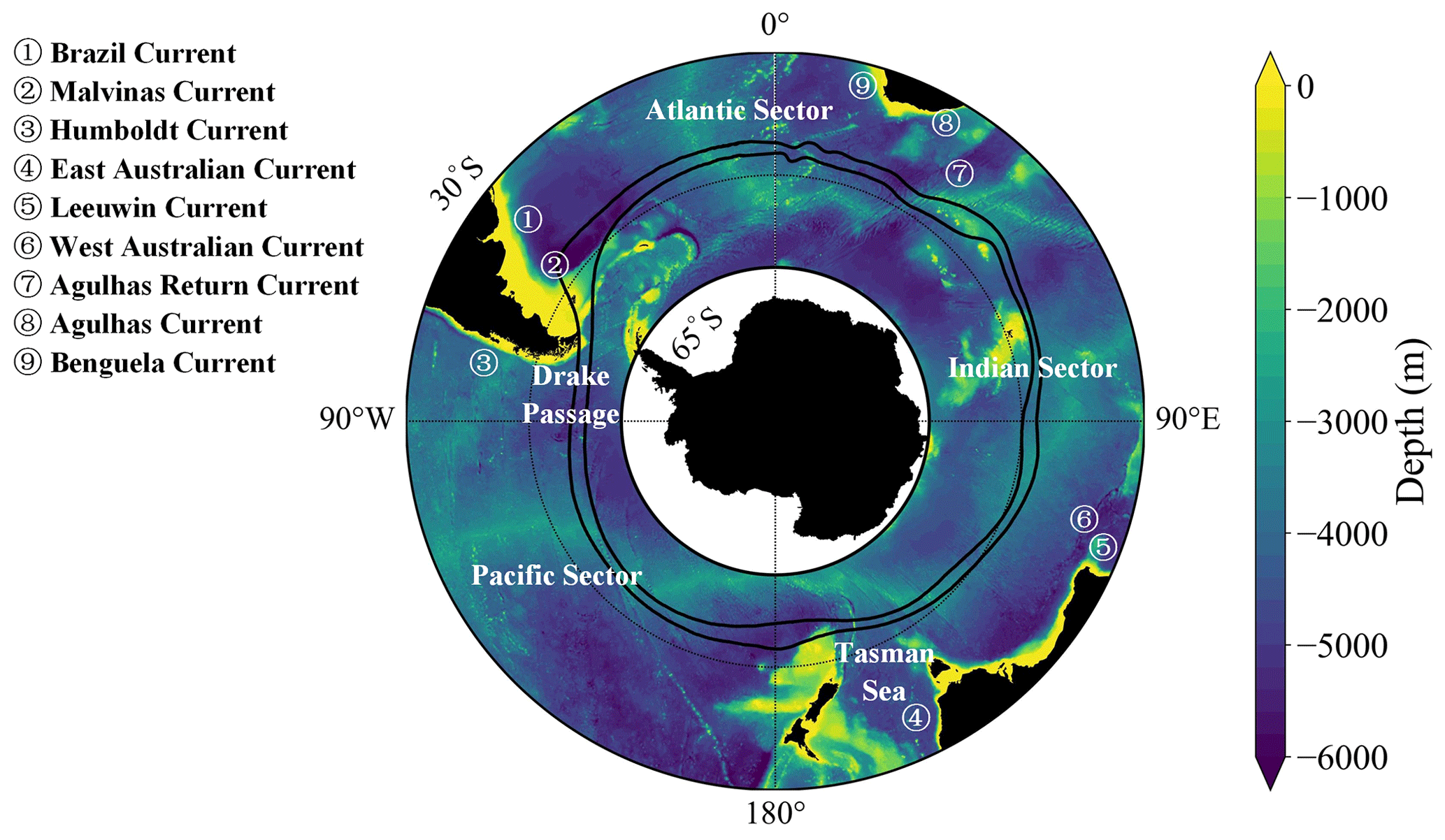
Figure 1Southern Ocean topography and current. The solid black solid lines show the mean northern (SAF) and southern (PF) positions of the ACC major fronts (Sallée et al., 2008). The dotted black circle is 50∘ S.
2.2 SST, Chl a, DIC, and pCO2 datasets
Four datasets of sea surface parameters are used in the study, including SST, Chl a, DIC, and pCO2 from 1996 to 2015, between 30 and 65∘ S. Table S1 presents information about spatial and temporal resolutions and filtering methods employed for these parameters. A brief description of each dataset is given below.
The daily SST dataset is the NOAA Optimum Interpolation (OI) SST product with 0.25∘ resolution, spanning from 1981 to the present (Reynolds et al., 2007). The SST dataset combines observations from different platforms on a regular global grid, including Advanced Very High-Resolution Radiometer (AVHRR) satellite data, ships, buoys, and Argo floats with an accuracy of about 0.1 ∘C daily.
The Chl a dataset is provided by the Copernicus Marine Environmental Monitoring Service (CMEMS), based on the Copernicus-GlobColour processor that merges three algorithms (Gohin et al., 2002; Hu et al., 2012; Garnesson et al., 2019). The Chl a dataset combines observations from different sensors (SeaWiFS (Sea-Viewing Wide Field-of-View Sensor), MODIS Aqua (Moderate Resolution Imaging Spectroradiometer on Aqua satellite), MODIS Terra (Moderate Resolution Imaging Spectroradiometer on Terra satellite), MERIS (MEdium Resolution Imaging Spectrometer), VIIRS NPP (Visible Infrared Imaging Radiometer Suite on the Suomi National Polar-orbiting Partnership satellite), VIIRS-JPSS1 (Visible Infrared Imaging Radiometer Suite on the Joint Polar Satellite System-1 satellite) OLCI-S3A, and S3B (Sentinel-3B satellite)). The original 4 km resolution data were re-gridded to 0.25∘ with daily temporal resolutions. We log-transform Chl a using the base 10 logarithm because Chl a is lognormally distributed (Campbell, 1995).
The pCO2 and DIC datasets are from the Japan Meteorological Agency (JMA) Ocean CO2 Map dataset with monthly 1∘ × 1∘ gridded values on the global ocean from 1990 to 2020 (Iida et al., 2021). The DIC concentration is calculated from total alkalinity (TA) values and CO2 fugacity (fCO2) data provided by the Surface Ocean CO2 Atlas (SOCAT), containing data from the 1950s to the present (Bakker et al., 2016). The DIC field is gap-filled by using a multi-linear regression (MLR) method based on the DIC and satellite observation data, including SST, sea surface salinity (SSS), sea surface dynamic height (SSDH), Chl a, and surface mixed layer depth (MLD) (Iida et al., 2021).
The globally averaged error in DIC is 6.1 µmol kg−1, which is 5.4 µmol kg−1 smaller than the error of the Global Ocean Data Analysis Project Version 2 update 2019 (GLODAPv2.2019), a uniformly calibrated open ocean data product on inorganic carbon and carbon-relevant variables (Olsen et al., 2019).
The pCO2 field is calculated from TA, DIC, SST, and SSS based on seawater CO2 chemistry (Iida et al., 2021). Firstly, the mean rates of regional pCO2 and multiple regressions are used to derive the algorithms of pCO2 expressed empirically as a function of in situ TA, DIC, SST, SSS, and the year. Then, the pCO2 fields that filled both in space (1∘ × 1∘) and time (monthly) are drawn by applying global datasets of TA, DIC, SST, and SSS to the variables in these empirical equations. The error in pCO2 was 10.9 µatm, comparable with that estimated with other empirical methods, e.g., 14.4 µatm (Landschützer et al., 2014) and 15.73 µatm (Denvil-Sommer et al., 2019). This dataset developed by Iida et al. (2021) is widely used to study the relationship between the pCO2 low-frequency variability and the recent global warming hiatus and the Interdecadal Pacific Oscillation, the net community production, and ocean acidification (Hashihama et al., 2021; Qiu et al., 2021; Ono et al., 2023).
2.3 Eddy database
Normal and abnormal eddies are from the eddy dataset developed by Liu et al. (2021) using a deep learning (DL) model based on the fusion of satellite sea surface height (SSH) and SST data. Based on the U-Net framework (Ronneberger et al., 2015; Falk et al., 2019), the model combines HyperDense-Net (Dolz et al., 2019) to fuse SSH and SST data. The SSH data used in the model are obtained from the Archiving, Validation, and Interpretation of Satellite Oceanographic data (AVISO) dataset. The SST data refer to the NOAA SST product (Reynolds et al., 2007). The model simultaneously extracts SSH anomaly (SSHA) features to determine eddy locations and distinguish between AEs and CEs and extracts the mean SST anomaly (SSTA) within eddy boundaries to distinguish between normal and abnormal eddies. Specifically, WAEs are identified according to SSHA > 0 and SSTA > 0, CAEs are identified according to SSHA > 0 and SSTA < 0, CCEs are identified according to SSHA < 0 and SSTA < 0, and WCEs are identified according to SSHA < 0 and SSTA > 0. The dice loss (a cost function to calculate the difference between the predicted and true values) and accuracy of the model was about 14 % and 94 % when training with the ground truth dataset, generated automatically using the SSH-based method (Liu et al., 2016). The eddy dataset has a daily and 0.25∘ resolution, including the number, radius, amplitude, rotational speed, and eddy kinetic energy (EKE) in the global ocean from 1996 to 2015. Due to the limitations of the resolution capability of the SSHA data (Ducet et al., 2000), eddies with amplitudes < 2 cm and radii < 35 km were discarded in this work.
Compared to the AVISO eddy database (Pegliasco et al., 2022), our study utilizes a different eddy detection method (Liu et al., 2021). The reason why we use this method is that DL technology has an unparalleled learning ability and the capability to model complex nonlinear relationships compared to traditional statistics and machine learning methods (Reichstein et al., 2019). Besides, our method achieves great accuracy and much higher efficiency than the traditional method that first detects the eddies and then uses the SST signature to classify them into normal and abnormal eddies (Liu et al., 2021). In addition, the method is able to detect eddies in regions where traditional methods may not be effective, such as in regions with weak eddies or regions with complex oceanic dynamics (Liu et al., 2021). Given its high accuracy and comprehensive information on eddy characteristics, we find this dataset particularly useful for our study. Considering that the changes in SSH, SST, Chl a, and roughness caused by eddies can be recorded by altimeter, infrared, ocean color, and synthetic aperture radar (SAR) remote sensing, respectively, and potential density and temperature recorded by Argo floats can also identify abnormal eddies, in future work, we will combine multiple remote sensing data with Argo profiles to evaluate the accuracies of abnormal eddy identification methods.
3.1 Composite eddy-induced anomalies
To extract the eddy-induced mesoscale features in sea surface variables, including SST, Chl a, DIC, and pCO2, we use temporal and spatial filters similar to those used in Villas Bôas et al. (2015) (Fig. S2). The temporal filter is a band-pass Butterworth window (Butterworth, 1930) applied to preserve the temporal signal between 7 and 90 d corresponding to the typical timescales of eddies. The SST and Chl a anomalies are computed using the 7–90 d band-pass filter to remove the seasonal signal. However, for DIC and pCO2 datasets with the monthly temporal resolution, we subtract their climatological averages. The spatial filter is a moving-average Hann window (Stearns and Ahmed, 1976) designed to contain spatial signals smaller than 600 km. This filter removes large-scale variability unrelated to the mesoscale eddy influence.
Finally, we use the eddy-centric composite method to estimate the spatial pattern of the eddy-induced anomalies in sea surface variables. The positions of co-located SST, Chl a, DIC, and pCO2 observations are normalized by R, which defines the edge of an eddy as ±1 and the eddy core as 0. This allows us to construct composite averages from eddies of various sizes. The specific method to calculate eddy-centric composite maps is demonstrated in Sect. S1. The composite maps are not rotated with the background variable gradient, as the large-scale background variable gradients in the SO are predominantly oriented north–south. Previous studies have indicated that rotating eddies to the large-scale variable gradient in the SO has a negligible impact on the results (Frenger et al., 2015). Therefore, the axes in each figure point north and east. This eddy-centric composite method is frequently used in studies of eddy tracer anomalies (Hausmann and Czaja, 2012; Gaube et al., 2013, 2014, 2015; Frenger et al., 2015; Dawson et al., 2018). Its advantage lies in the ability to average over multiple eddies, which helps reduce noise and reveal persistent eddy structures (Melnichenko et al., 2017). This method is particularly useful when studying eddies in regions where eddy activity is highly variable, as it allows us to identify common patterns and trends in eddy-induced anomalies.
3.2 Eddy-induced Ekman pumping
At present, there are no explicit formulas to quantify eddy stirring, trapping, and pumping, but with the Ekman transport modified by the surface geostrophic vorticity ζ following Stern (1965) the total eddy-induced Ekman pumping Wtot is
where ρo=1020 kg m−3 is the (assumed constant) density of sea surface water; f is the Coriolis parameter; and the surface stress τ has the zonal and meridional components τx and τy, respectively. The surface stress curl ∇×τ was computed by using finite centered differences of τx and τy. The surface geostrophic vorticity ζ is calculated as
where u and v are the zonal and meridional components of geostrophic current velocity. The surface wind stress τ is calculated as
where ρa=1.2 kg m−3 is the air density (assumed constant); CD is the drag coefficient; and Ua and Uo are the wind and ocean current vectors, respectively. The above formulas used to calculate the Wtot are similar to those used in Gaube et al. (2015).
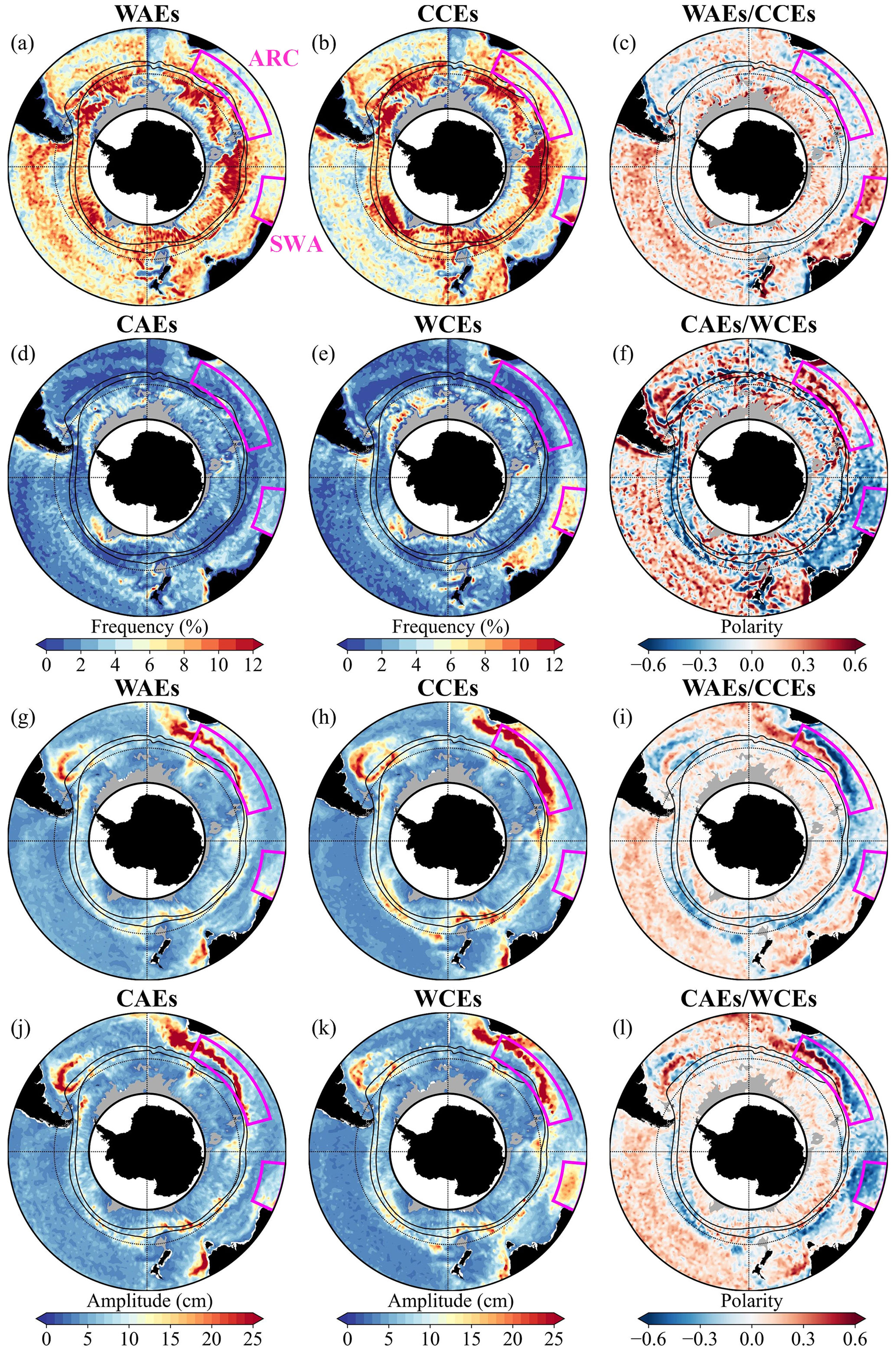
Figure 2Spatial distribution of (a), (b), (d), and (e) eddy frequency; (g), (h), (j), and (k) eddy amplitude; and eddy polarity dominance in the SO from 1996 to 2015. (c, f) Ratio of the area occupied by WAEs/CAEs over the area covered by CCEs/WCEs. (i, l) Ratio of amplitude for WAEs/CAEs over CCEs/WCEs. For (c), (f), (i), and (l) eddy polarity, values > 0 in red and < 0 in blue mark the dominance of AEs and CEs, respectively. Black solid lines show the mean northern (SAF) and southern (PF) positions of the ACC major fronts (Sallée et al., 2008). The black dotted circle is 50∘ S. The magenta boxes represent the Agulhas Return Current (ARC) and southwestern Australia (SWA) regions.
Ua is a gridded Level 4 (L4) product with 0.25∘ resolution available every 6 h from the Cross-Calibrated Multi-Platform (CCMP) ocean surface wind dataset, produced by remote sensing systems. The dataset combines ocean surface (10 m) wind retrievals from a reanalysis background field from the ERA-Interim reanalysis, multiple types of satellite microwave sensors, and observations from ships and buoys. The Uo is a daily sea surface geostrophic current product with a spatial 0.25∘ resolution obtained from AVISO.
To extract the mesoscale features of Wtot, we use temporal and spatial filters similar to those used in Gaube et al. (2015). The Wtot is temporally low-pass filtered with a half-power filter cutoff of 30 d and spatially high-pass filtered to contain spatial signals smaller than 600 km. Finally, we use the eddy-centric composite method to obtain the spatial pattern of eddy-induced Ekman pumping.
4.1 Spatial distributions of normal and abnormal eddies
From 1996 to 2015, an average of 1991 eddies were identified daily in the SO (65–30∘ S), with abnormal eddies accounting for 26.3 % of the total. Figure 2a, b, d, and e show the spatial distribution of the eddy number, defined as the frequency of eddy occurrence in each 1∘ × 1∘ latitude–longitude bin over the analyzed period of 1996–2015. The eddy frequency represents the ratio of the number of days the eddies appeared to the total number of observation days. Eddies disappear in the regions shallower than 2000 m and the area near Antarctica (shown in gray in Fig. 2) because the bottom topography constrains the generation of eddies, and satellite altimetry cannot measure sea level beneath sea ice (Frenger et al., 2015). Normal and abnormal eddies are concentrated in strong current regions, such as the ACC, Western Boundary Current (WBC), and Eastern Boundary Current (EBC) regions, as shown in Fig. 1. These findings are consistent with those findings reported by Frenger et al. (2015), which did not distinguish between normal and abnormal eddies. The differences between AEs and CEs, i.e., the eddy polarity, are critical for understanding the physical and biogeochemical anomalies induced by eddies (McGillicuddy et al., 1998; Siegel et al., 2011). Abnormal eddies have the opposite polarity distribution to normal eddies in the continental boundary currents where more CCEs and CAEs occur. The most significant difference in polarity distributions between normal and abnormal eddies is the dominance of WAEs and WCEs in the southwestern Australia (SWA) region (Fig. 2c, f).
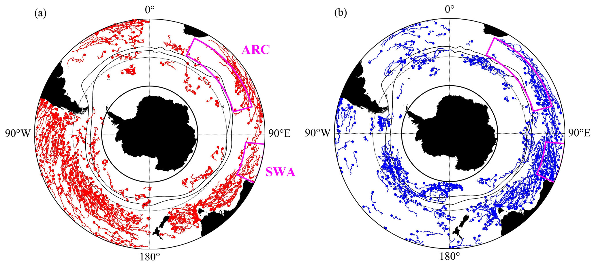
Figure 3Trajectories of (a) AEs and (b) CEs in the SO during 1996–2015. Red (blue) dots and lines mark the AEs (CEs) birth locations and propagation paths. To show the eddy tracks more clearly, only eddies with a minimum lifetime of 1 year and one-third of the long-lived eddies in the south and southwest of Australia have been considered. The solid black lines show the mean northern (SAF) and southern (PF) positions of the ACC major fronts (Sallée et al., 2008). The dotted black circle is 50∘ S. The magenta boxes represent the ARC and SWA regions.
Despite the great differences in occurrence distributions, the amplitude distributions of the four types of eddies are similar. The eddy amplitude is greater in the Brazil–Malvinas Confluence (BMC), Agulhas Return Current (ARC), ACC, SWA, and Tasman Sea regions (Fig. 2g, h, j, and k). One should note that the amplitudes of abnormal eddies are smaller than those of normal ones (Table S2), which is consistent with previous studies (Liu et al., 2020, 2021). In addition, the spatial distributions of rotational speed and EKE correlate well with the patterns of eddy amplitude (Fig. S3).
We investigated the tracks of normal and abnormal eddies and found that they are consistent (Fig. 3 and Table S3). To accurately represent eddy propagation directions, we incorporated statistics that encompass a broader range of eddy lifetimes, including both short-lived and long-lived eddies (living longer than 1 year) (Table S3). Regardless of the lifespan, both AEs and CEs propagate primarily westward and northward. By contrast, AEs and CEs with lifetimes longer than 1 year propagate primarily northward and southward, respectively, corresponding with the intrinsic meridional propagation of eddies (Cushman-Roisin and Beckers, 2011). Frenger et al. (2015) reported that only partial eddies follow this intrinsic meridional propagation in the SO, owing to the strong overcompensation by the background meridional deflections of the mean current. Figure 3 shows that between 30∘ S and the ACC the major propagation direction of eddies is westward, with AEs propagating north and CEs propagating south. However, most eddies in the ACC influence area propagate eastward, with AEs propagating south and CEs propagating north. These results are similar to those reported by Dawson et al. (2018).
4.2 Spatial distributions of eddy-induced SST, Chl a, DIC, and pCO2 anomalies
Using the eddy-centric composite method (Fig. S2), we average the eddy-induced SST, Chl a, DIC, and pCO2 anomalies into 1∘ × 1∘ longitude–latitude grid boxes. The maps of the climatological imprint of eddies on SST show that the distributions of SST anomalies over normal eddies correlate well with the amplitude distributions, with stronger positive/negative SST anomalies (in WAEs/CCEs) concentrated in the BMC, ARC, ACC, SWA, and Tasman Sea regions (Fig. 4a, c). In contrast, in regions with larger amplitudes, CAEs/WCEs have weaker negative/positive SST anomalies (Fig. 4b, d).
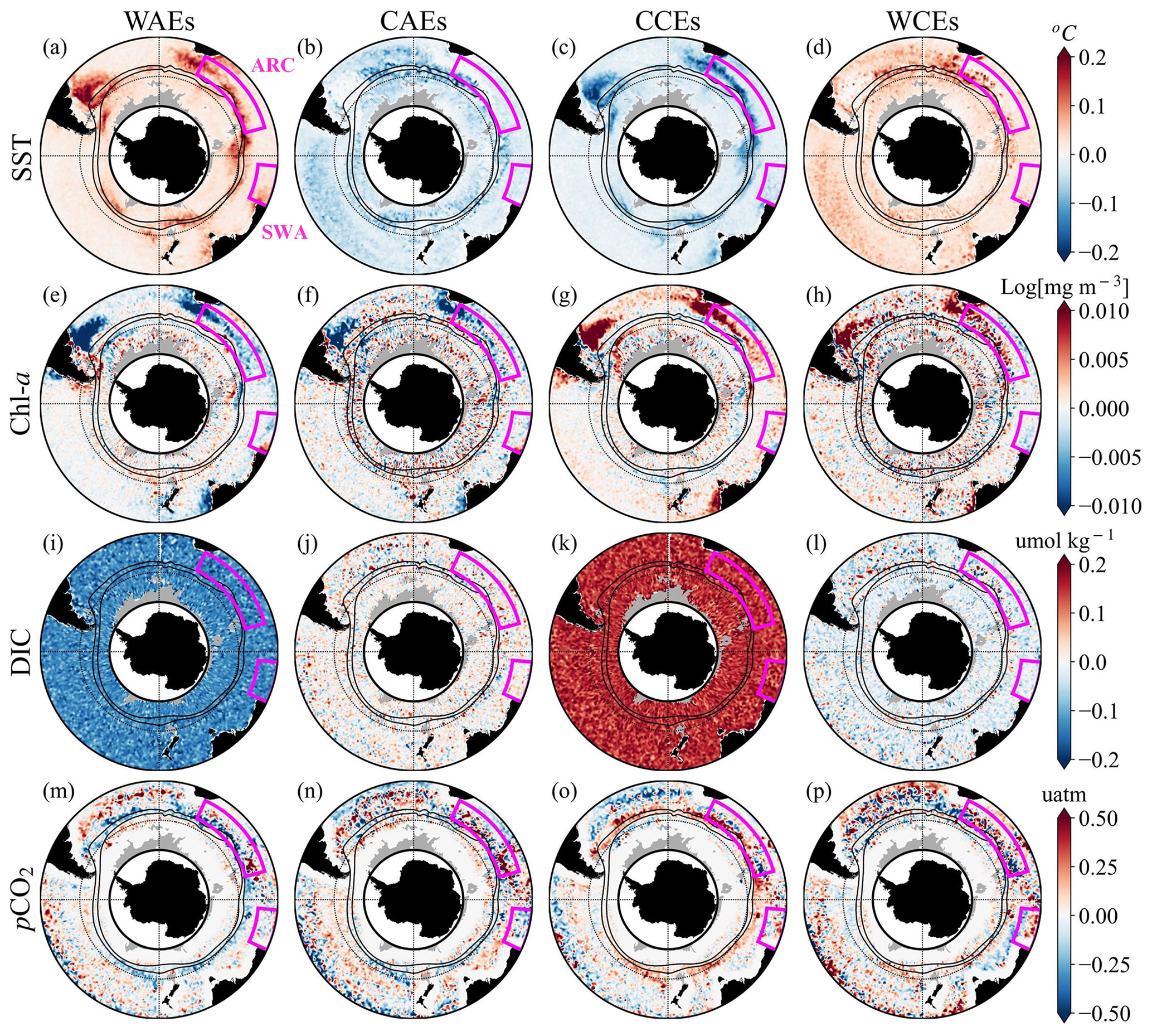
Figure 4Spatial distribution of eddy-induced anomalies of (a–d) SST, (e–h) Chl a, (i–l) DIC, and (m–p) pCO2 in the Southern Ocean from 1996 to 2015. The anomalies within eddies are averaged in 1∘ × 1∘ longitude–latitude grid boxes. From left to right, the columns represent four kinds of eddies. The solid black lines show the mean northern (SAF) and southern (PF) positions of the ACC major fronts (Sallée et al., 2008). The dotted black circle is 50∘ S. The magenta boxes represent the ARC and SWA regions.
Also, the distributions of Chl a anomalies over both normal and abnormal eddies are similar to the amplitude distributions, with stronger negative/positive anomalies within AEs/CEs in regions with higher amplitudes (Fig. 4e–h). However, in the south of the ACC, including the ACC, we find that the patterns of Chl a anomalies appear spotty, with average positive and negative Chl a anomalies in AEs and CEs, respectively. As shown in Fig. S4, the correlation coefficients between amplitude and Chl a anomalies have larger magnitudes in subtropical waters, with negative values in WAEs and CAEs and positive values in CCEs and WCEs. This result illustrates that in subtropical regions with higher amplitudes, such as the BMC, ARC, and Tasman Sea, WAEs and CAEs induced stronger negative Chl a anomalies, while CCEs and WCEs induced stronger positive Chl a anomalies.
The distributions of DIC anomalies differ significantly from those of SST and Chl a anomalies, with uniform speckles featuring average negative DIC anomalies in WAEs and WCEs and positive DIC anomalies in CAEs and CCEs (Fig. 4i–l). In addition to the opposite DIC anomaly signals between normal and abnormal eddies, the magnitudes of DIC anomalies are generally larger in normal eddies than in abnormal eddies.
The patterns of eddy-induced pCO2 anomalies are zonal. For AEs, pCO2 anomalies are positive in the north of ACC and negative along the ACC, while the opposite is true for CEs (Fig. 4m–p). However, there are some distinctions between normal and abnormal eddies. For example, in the north of the ACC (including SWA) with high SST (Fig. 5a1) and low DIC (Fig. 5b1), WAEs and WCEs have more positive speckles compared to CAEs and CCEs, respectively. Conversely, along the ACC (including ARC) with low SST (Fig. 5a1) and high DIC (Fig. 5b1), WAEs and WCEs have more negative speckles than CAEs and CCEs.
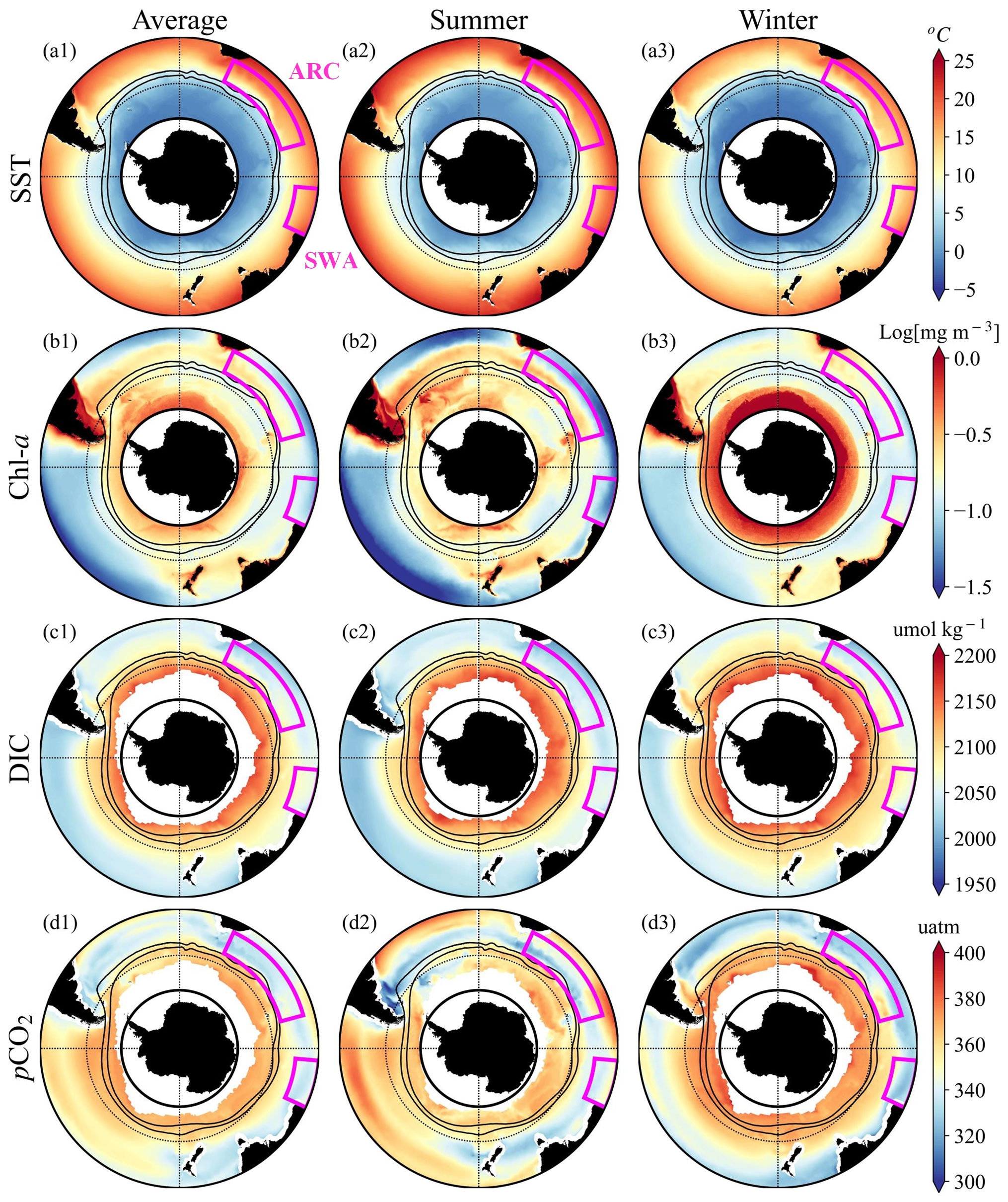
Figure 5The climatological and seasonal averages of (a1–a3) SST, (b1–b3) Chl a, (c1–c3) DIC, and (d1–d3) pCO2 from 1996 to 2015 in the SO. The solid black lines show the mean northern (SAF) and southern (PF) positions of the ACC major fronts (Sallée et al., 2008). The dotted black circle is 50∘ S. The magenta boxes represent the ARC and SWA regions.
These findings indicate variability in the spatial distribution of physical and biogeochemical parameters induced by normal and abnormal eddies. To further quantify the effects of eddies on different parameters, we average all eddy-centric composite maps for SST, Chl a, DIC, and pCO2 anomalies over eddies to analyze the pattern characteristics of eddy-induced parameters. Due to seasonal variations in pCO2, the eddies' physical and biogeochemical characteristics are also synthesized in summer and winter.
4.3 Composite maps of eddy-induced SST, Chl a, DIC, and pCO2 anomalies
Using the eddy-centric composite method (Fig. S2), we investigate the seasonal variations of SST, Chl a, DIC, and pCO2 associated with normal and abnormal eddies in the SO (Fig. 6). Figure 6a1–a4 and e1–e4 show the composite SST anomalies within normal and abnormal eddies in winter and summer, respectively. There are no significant differences in the signals and spatial patterns of SST anomalies within the same kind of eddies between summer and winter. Composite SST anomalies over normal eddies show asymmetric monopole patterns, with positive/negative extrema slightly shifting westward and poleward (equatorward) relative to the WAE/CCE cores. In comparison, abnormal eddies also display monopole patterns but with opposite signals. Furthermore, the magnitudes of SST anomalies over normal eddies are larger than those over abnormal eddies.
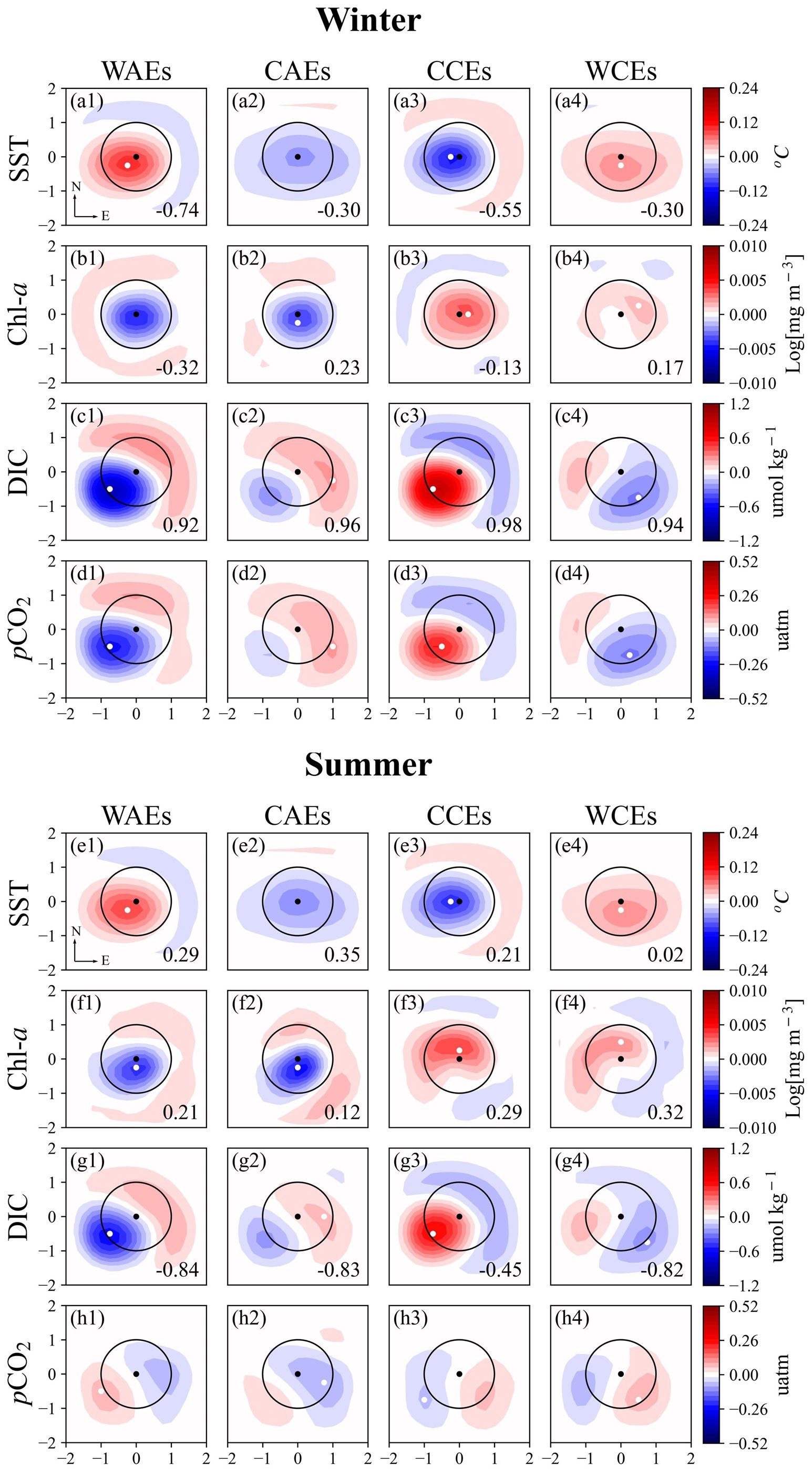
Figure 6Eddy-centric composite averages for SST, Chl a, DIC, andpCO2 anomalies in the SO. On each map, a black dot denotes the eddy center, and a white dot denotes the center location of variables (defined by the location of the extremum value). Contour intervals are every 0.009 ∘C for SST, every 0.0007 Log[mg m−3] for Chl a, every 0.08 µmol kg−1 for DIC, and every 0.035 µatm for pCO2. The numbers in the lower right corner are the structural similarity indexes (SSIMs).
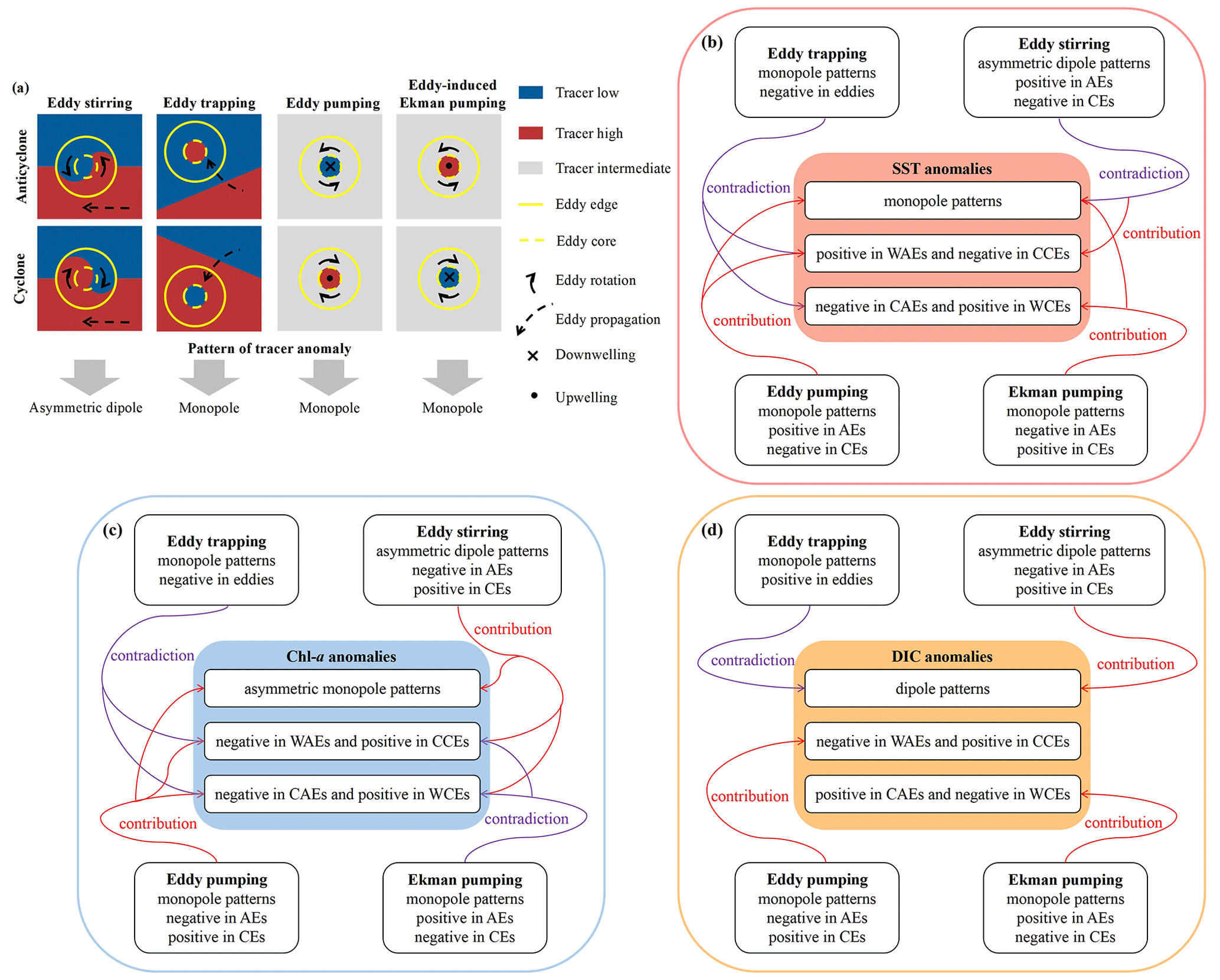
Figure 7(a) Schematic illustrating the mechanisms of how eddies affect physical and biogeochemical parameters in the SO, including eddy stirring, eddy trapping, eddy pumping, and eddy-induced Ekman pumping. The patterns of SST anomalies induced by vertical pumping are opposite to the corresponding patterns shown in this schematic. The figure is inspired by Frenger et al. (2018), Fig. 1. A schematic diagram of the eddy mechanisms influencing (b) SST, (c) Chl a, and (d) DIC anomalies.
The composite Chl a anomalies within the same kind of eddies also show no obvious seasonality in the signals and spatial patterns (Fig. 6b1–b4 and f1–f4). Moreover, composite Chl a anomalies have no significant difference between normal and abnormal eddies, with monopole negative signals in WAEs and CAEs and positive signals in CCEs and WCEs. The extrema of Chl a anomalies shift slightly poleward relative to the cores of WAEs and CAEs and equatorward relative to the cores of CCEs and WCEs.
Regarding eddy-induced DIC anomalies, their composite maps within the same kind of eddies are similar in summer and winter, except that the magnitudes of DIC anomalies within eddies are slightly higher in winter (Fig. 6c1–c4 and g1–g4). Moreover, the composite DIC anomalies within normal and abnormal eddies show dipole patterns dominated by opposite signals. WAEs are dominated by negative DIC anomalies, whereas CAEs are dominated by positive DIC anomalies. CCEs are dominated by positive DIC anomalies, whereas WCEs are dominated by negative DIC anomalies. The DIC anomalies have opposite signals to SST anomalies within the same kind of eddies.
Although pCO2 is influenced by SST, Chl a, and DIC, pCO2 anomalies within eddies in winter are significantly different from summer, unlike SST, Chl a, and DIC anomalies within eddies similar in summer and winter (Fig. 6d1–d4 and h1–h4). To determine which factor dominates the change in pCO2, we calculate the structural similarity index (SSIM) in Eq. (5), which can quantify the similarity of the patterns between pCO2 and other anomalies over eddies (Wang et al., 2004).
where X and Y denote the composite averages of normalized pCO2 and DIC (SST) anomalies, respectively. μX and μY are the average values of X and Y. σX and σY are the standard deviations of X and Y. σXY is the covariance of X and Y. Lp is the dynamic range of values, Lp=2. k1=0.01 and k2=0.03. SSIM ranges from −1 to 1. The closer the SSIM value is to 1, the more similar the two patterns are. Because the Chl a negatively correlates with the pCO2, its SSIMs are multiplied by −1. In winter, the SSIMs between pCO2 and DIC anomalies are the largest (>0.9). The pCO2 anomalies have similar patterns and signals with DIC anomalies, dominant by positive signals within CAEs and CCEs and negative signals within WAEs and WCEs (Fig. 6d1–d4). However, in summer, the SSIMs are negative between pCO2 and DIC anomalies but positive between pCO2 and SST (Chl a) anomalies over eddies in summer (≤0.35). The patterns of pCO2 anomalies differ from those of SST, Chl a, and DIC within eddies in the SO (Fig. 6h1–h4).
This section discusses how eddies affect SST, Chl a, DIC, and pCO2 through various mechanisms, including eddy stirring, trapping, pumping, and eddy-induced Ekman pumping (Fig. 7).
5.1 Mechanism analysis of eddy's influence on SST
Composite SST anomalies over eddies show monopole patterns, with positive anomalies in WAEs and WCEs and negative anomalies in CCEs and CAEs (Figs. 6a1–a4, 6e1–e4, and S5a and Table S4). First, we analyze the effect of eddy trapping on SST, which is determined by the directions of the horizontal SST gradient and eddy propagation (Frenger et al., 2015, 2018). The climatological and seasonal averages of SST reveal a zonal distribution with a southward decrease (Fig. 5a1–a3). Table S3 shows that the predominant propagation direction of eddies is westward and northward (Fig. 3). According to the southward decreasing SST, northward propagating eddies would trap cold water and result in negative SST anomalies. However, this process contradicts the positive SST anomalies within WAEs and WCEs, indicating the weak effect of eddy trapping on SST.
The meridional and zonal phase shifts in normal eddies are proposed to be induced by the large-scale background SST gradient and eddy stirring (Hausmann and Czaja, 2012; Villas Bôas et al., 2015). Specifically, WAEs rotating counterclockwise through the SST gradient would advect warmer water from the north to the southeast, leading to positive extrema slightly shifting westward and poleward relative to the cores (Fig. 6a1, e1). Conversely, CCEs rotating clockwise through the SST gradient would advect cooler water from the south to the northwest, leading to negative extrema slightly shifting westward and equatorward relative to the cores (Fig. 6a3, e3). In summary, for the advective effects of eddies, the effect of eddy trapping on SST is not reflected, and eddy stirring contributes to the slight shift of SST anomaly extrema within normal eddies.
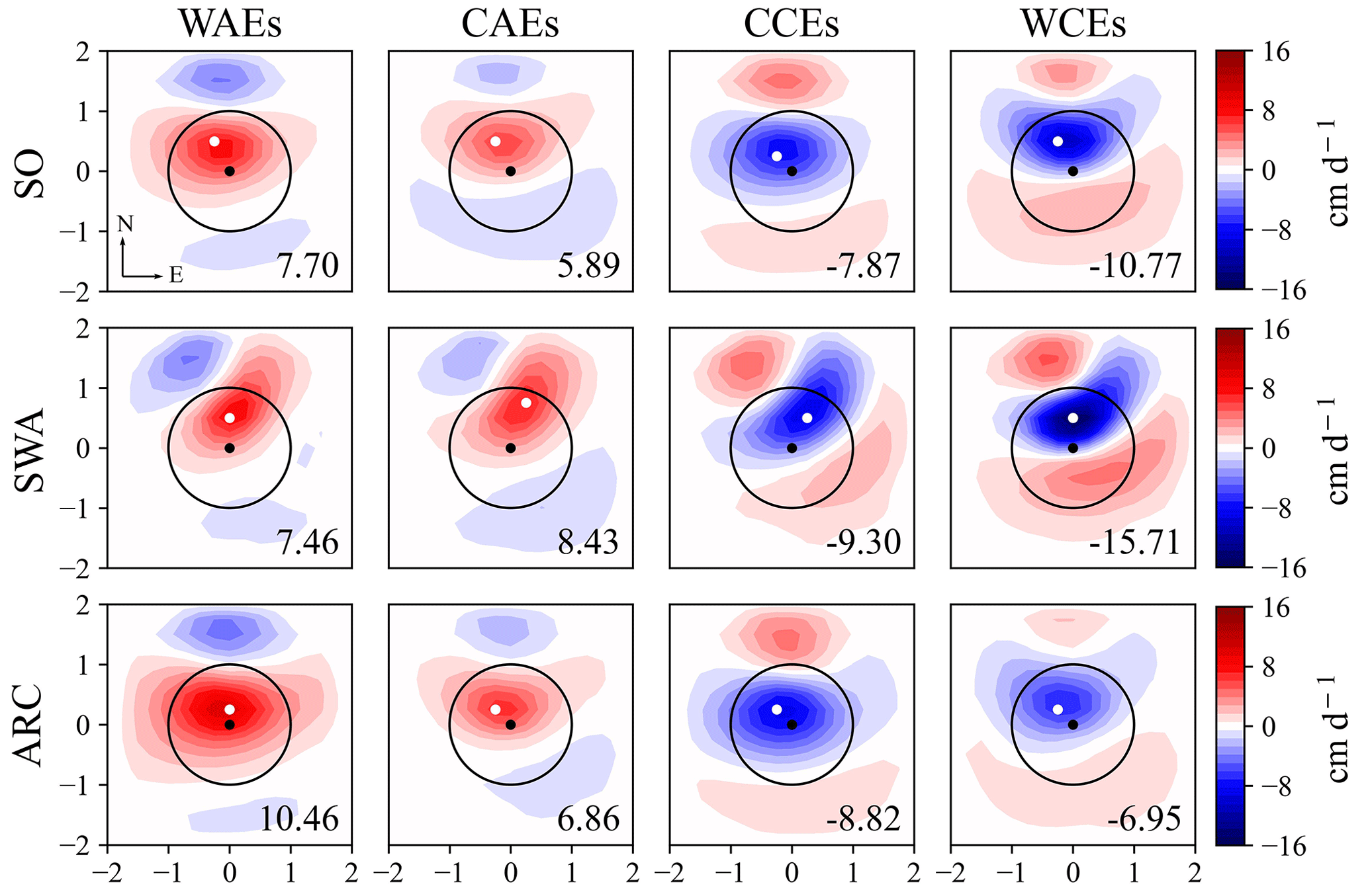
Figure 8Eddy-centric composite averages for eddy-induced Ekman pumping in the SO, SWA, and ARC regions. On each map, a black dot denotes the eddy center, and a white dot denotes the center location of variables (defined by the location of the extremum value). Contour intervals are 1.067 cm d−1. The numbers in the lower right corner are the extremum value.
For the vertical effects of eddies, eddy pumping within AEs associated with downwelling induces positive SST anomalies, while eddy pumping within CEs associated with upwelling induces negative SST anomalies (Fig. 7b). This process is consistent with the observed SST anomalies within normal eddies (Fig. 6a1, a3, e1, and e3). On the other hand, eddy-induced Ekman pumping within AEs associated with upwelling induces negative SST anomalies, while eddy-induced Ekman pumping within CEs associated with downwelling induces positive SST anomalies (Fig. 7b) (Gaube et al., 2013; Dawson et al., 2018). This process is consistent with the observed SST anomalies within abnormal eddies (Fig. 6a2, a4, e2, and e4). Moreover, WAEs/CCEs have stronger positive/negative SST anomalies in the regions with larger amplitudes, while CAEs/WCEs have weaker negative/positive SST anomalies (Fig. 4a–d). We further compared the quantitative relationship between SST anomalies and amplitudes over normal and abnormal eddies, as shown in Fig. S6. The SST anomalies in WAEs and CAEs are positively correlated with amplitudes, whereas the SST anomalies in CCEs and WCEs are negatively correlated with amplitudes. These findings indicate that the strength of eddy pumping is positively correlated with eddy amplitude, i.e., a larger amplitude corresponds to stronger downwelling and upwelling in the cores of AEs and CEs, respectively. Table S2 shows that the amplitudes of abnormal eddies are smaller than normal eddies, indicating weaker eddy pumping in abnormal eddies. Hence, abnormal eddies are more likely to be influenced by eddy-induced Ekman pumping. In summary, within normal eddies, eddy pumping dominates the vertical heat advection, resulting in positive SST anomalies in WAEs and negative SST anomalies in CCEs (Fig. 6a1, a3, e1, and e3). However, within abnormal eddies, the effect of eddy-induced Ekman pumping becomes more prominent, resulting in negative SST anomalies in CAEs and positive SST anomalies in WCEs (Fig. 6a2, a4, e2, and e4).
5.2 Mechanism analysis of an eddy's influence on Chl a
The composite maps of eddy-induced Chl a anomalies in the SO show asymmetric monopole patterns, with negative/positive extrema shifting poleward/equatorward relative to the AE/CE cores (Fig. 6b1–b4 and f1–f4). We calculate the climatological average gradient of Chl a in the SO from 1996 to 2015, which is normalized before calculation. The north–south gradient of Chl a is −0.02 (north is the positive direction), and the east-west gradient of Chl a is −0.04 (east is the positive direction). Due to the climatological Chl a increasing southward (Fig. 5b1–b3), eddies propagating northward tend to trap high Chl a into northern areas with low Chl a. Likewise, due to the climatological Chl a increasing westward, eddies propagating westward tend to trap low Chl a into western areas with high Chl a. However, the effect of eddy trapping on Chl a cannot explain the opposite Chl a anomalies between AEs and CEs (Fig. 6b1, b2, f1, and f2). Consequently, it can be inferred that the role of eddy trapping in influencing Chl a distributions is limited.
Moreover, considering that the climatological Chl a increases southward and westward, the counterclockwise rotation of AEs in the SO would advect low Chl a from the northeast to the west and high Chl a from the southwest to the east. The reverse is true for CEs. Previous works found that the dipole shapes arising from stirring tend to be asymmetric, with larger anomalies on the leading side compared to the trailing side of eddies (Fig. 7a, c) (Chelton et al., 2011b; Frenger et al., 2015, 2018; Dawson et al., 2018). As the major propagation direction of eddies is westward (Table S3), the composite Chl a anomalies in AEs/CEs show dominant negative/positive signals due to eddy stirring (Fig. 6b1–b4 and f1–f4). Like SST anomaly patterns, Chl a anomaly patterns also show meridional and zonal extremum shifts. For meridional shifts, AEs rotating counterclockwise through the southward-increasing Chl a gradient would induce negative extrema slightly shifting poleward relative to the cores (Fig. 6b2, f1, and f2). The reverse is true for CEs (Fig. 6b3, b4, f3, and f4). For zonal shifts, AEs through the westward increasing Chl a gradient would induce negative extrema shifting slightly westward relative to the cores (Fig. 6b2, f1, and f2). The reverse is true for CEs (Fig. 6b3, b4, f3, and f4).
Eddy pumping induces negative and positive Chl a anomalies within AEs and CEs, respectively; on the contrary, eddy-induced Ekman pumping induces positive and negative Chl a anomalies within AEs and CEs, respectively (Dawson et al., 2018). The eddy-centric composite maps of Chl a anomalies show monopole negative signals in AEs and positive signals in CEs (Fig. 6b1–b4 and f1–f4). Besides, in regions of higher amplitude, the magnitudes of eddy-induced Chl a anomalies are greater (Fig. 4e–h). These results reflect the dominant effect of eddy pumping on Chl a anomalies within eddies. However, the more evident Ekman pumping mechanism of abnormal eddies resists eddy pumping and leads to a lower Chl a magnitude within abnormal eddies than normal eddies (Fig. 6b1–b4 and f1–f4). It is worth noting that in some regions with small amplitudes, such as the south of ACC and the south Pacific Ocean, we observe positive Chl a anomalies in AEs and negative Chl a anomalies in CEs (Fig. 4e–h). Such a result may be caused by a more dominant effect of eddy-induced Ekman pumping on Chl a. Overall, eddy stirring and eddy pumping are mainly responsible for the patterns of Chl a anomalies within eddies in the SO, and eddy-induced Ekman pumping attenuates the magnitudes of Chl a anomalies within abnormal eddies.
5.3 Mechanism analysis of an eddy's influence on DIC
The composite DIC anomalies within normal and abnormal eddies show dipole patterns with opposite dominant signals, negative in WAEs and WCEs and positive in CAEs and CCEs in the SO (Figs. 6c1–c4, 6g1–g4, and S5c and Table S4). Due to the climatological DIC increasing southward, the counterclockwise rotation of AEs in the SO would advect low DIC from the north to the southwest and high DIC from the south to the northeast. The reverse is true for CEs. As eddies migrate westward, negative and positive DIC anomalies in AEs and CEs on the western side would intensify, affected by asymmetric dipole shapes arising from eddy stirring (Fig. 7a, d). Under the condition of southward-increasing DIC (Fig. 5c1–c3), eddies propagating northward tend to trap high DIC. Thus, the effect of eddy trapping may contribute to the positive signals of DIC anomalies within eddies. However, the opposite dominant signals between normal and abnormal eddies cannot be explained solely by the advective effects of eddies.
Eddy pumping induces negative DIC anomalies within AEs through the downwelling of surface low-DIC waters and positive DIC anomalies within CEs through the upwelling of deep DIC-rich waters. The reverse is true for the effect of eddy-induced Ekman pumping on DIC anomalies. As mentioned in Sect. 5.1, the greater amplitude of eddies corresponds to stronger eddy pumping. The larger amplitude of normal eddies than abnormal eddies leads to higher magnitudes of negative DIC anomalies in WAEs and positive anomalies in CCEs. Moreover, the Ekman pumping caused by WAEs is stronger than that caused by CAEs (Fig. 8a1, a2), resulting in stronger positive DIC anomalies within WAEs than CAEs (Fig. 6c1, c2, g1, and g2). Similarly, the Ekman pumping caused by WCEs is stronger than that caused by CCEs (Fig. 8a3, a4), resulting in stronger negative DIC anomalies within WCEs than CCEs (Fig. 6c3, c4, g3, and g4). Consequently, the combined effects of eddy pumping and eddy-induced Ekman pumping contribute to the dominant negative DIC anomalies within WAEs and WCEs and positive DIC anomalies within CAEs and CCEs in the SO.
5.4 Mechanism analysis of an eddy's influence on pCO2
In winter, the pCO2 anomalies have similar patterns and signals to DIC anomalies, and the SSIMs between pCO2 and DIC anomalies are the highest in the SO (Fig. 6d1–d4), suggesting that the effect of DIC on pCO2 is stronger than the effects of SST and Chl a. However, in summer, the patterns of pCO2 anomalies differ significantly from the anomalies of SST, Chl a, and DIC within eddies in the SO with relatively lower SSIMs (the highest SSIM is 0.35) (Fig. 6h1–h4). This result may be caused by different processes affecting pCO2 in different regions of the SO. To prove this hypothesis, we further examine the eddy-induced SST, Chl a, DIC, and pCO2 anomalies in the SWA (95–115∘ E, 30–40∘ S) and ARC (25–75∘ E, 35–45∘ S) regions, where the eddy activity is strong, and the eddy amplitude and rotation speed are high (Figs. 2, S3, rectangular magenta box), leading to strong eddy stirring, trapping, and pumping (Dawson et al., 2018; Frenger et al., 2018).
Similar to the SO, the SSIMs between the pCO2 and DIC anomalies are the highest in both the SWA and ARC regions during winter, indicating the dominant effect of DIC on pCO2 (Figs. 9d1–d4 and 10d1–d4). However, unlike the SO, the SSIMs between the pCO2 and SST anomalies are the highest in the summer SWA region (Fig. 9h1–h4). By contrast, the SSIMs between pCO2 and DIC anomalies are the highest in the summer ARC (Fig. 10h1–h4). These results suggest that in summer, the pCO2 within eddies is dominated by the SST effect in the SWA region and dominated by the DIC effect in the ARC. Despite similar magnitudes of SST anomalies over eddies between the SWA and ARC regions, the magnitudes of DIC anomalies in the SWA region are significantly lower than those in the ARC, which may cause different processes affecting pCO2 in these two regions. Likewise, the pCO2 anomalies over eddies are determined by the DIC anomalies in winter, which is also associated with the higher magnitudes of DIC anomalies in winter compared to summer (Fig. 6c1–c4 and g1–g4). Such regional and seasonal magnitude variations of DIC anomalies are controlled by the complex interactions among processes such as biological activity (production/remineralization), vertical mixing, and air–sea gas exchanges (Racapé et al., 2010).
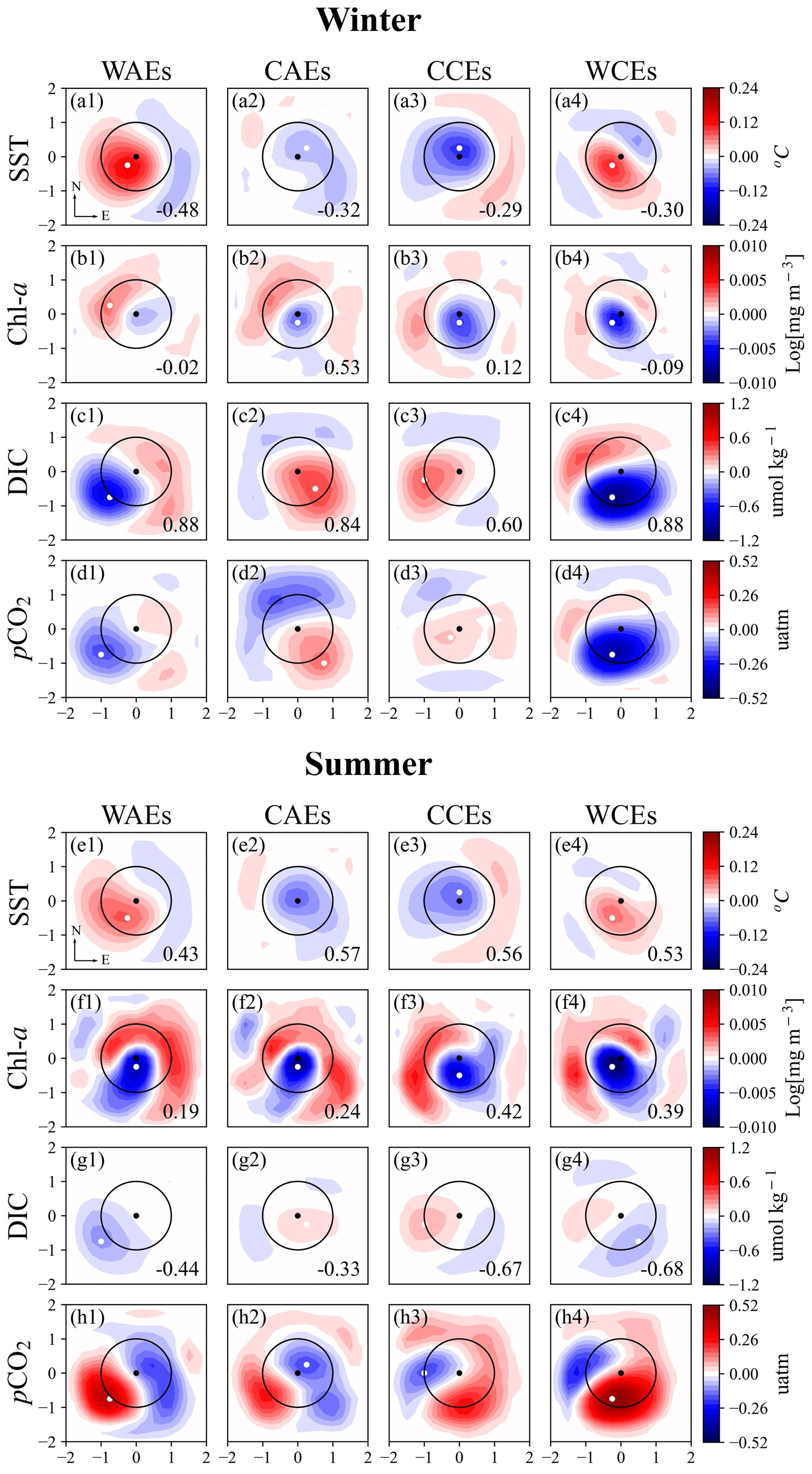
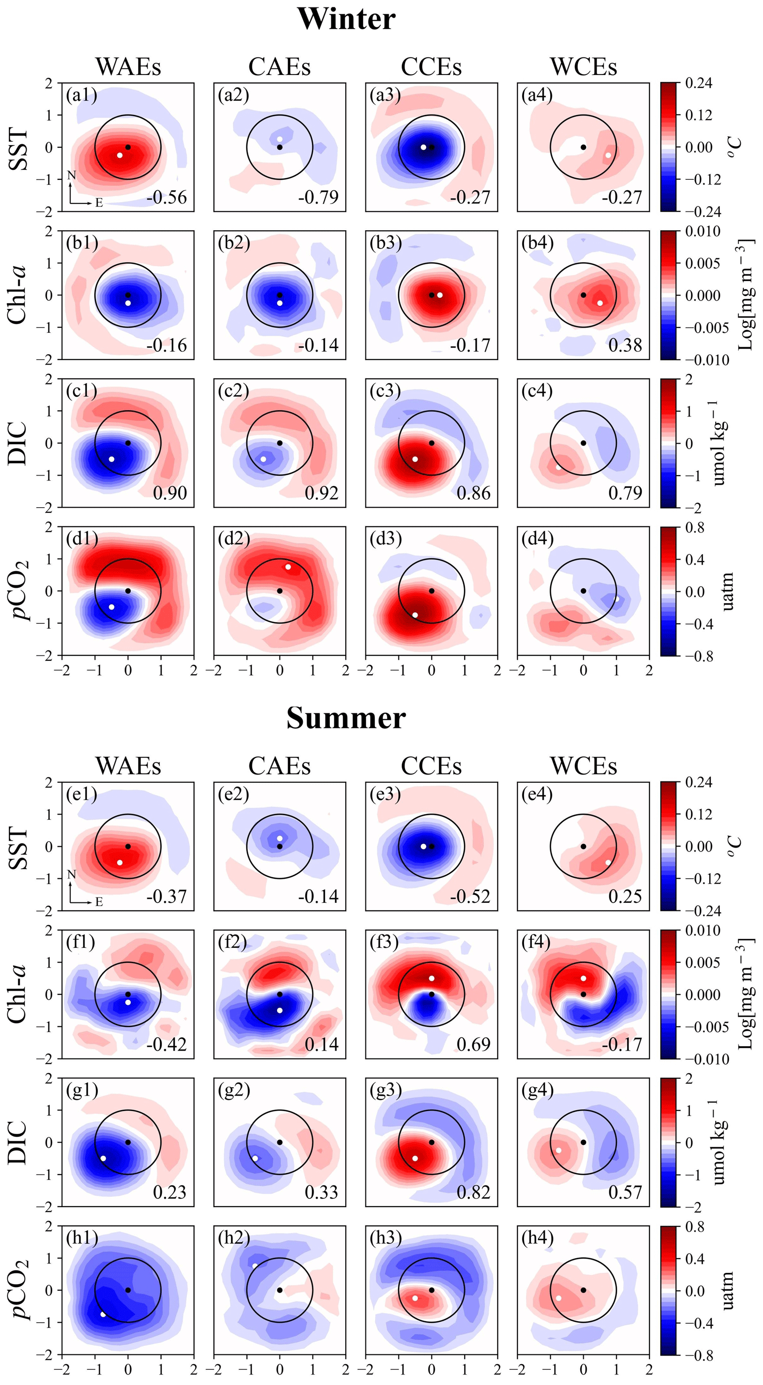
Figure 10Same as Fig. 6 but for the ARC. And contour intervals are every 0.133 µmol kg−1 for DIC and every 0.053 µatm for pCO2.
We further calculate the contributions of eddies to pCO2 (Table S5). On average, the contributions of abnormal eddies to pCO2 are generally smaller than those of normal eddies in the SO and ARC. Nevertheless, the contributions of abnormal eddies to pCO2 surpass those of normal eddies in the SWA region. These findings can be attributed to the dominance of abnormal eddies in the SWA region, primarily driven by the more pronounced eddy-induced Ekman pumping observed in abnormal eddies as compared to normal eddies (Figs. 2, 8). This contrast in Ekman pumping between abnormal and normal eddies is more significant in the SWA region than in the SO and ARC regions, as illustrated in Fig. 8. Additionally, the contributions of the ARC and SWA eddies to pCO2 are higher than the SO eddies, which is caused by the regional cancellation effect in the SO (Fig. 4m–p). In the SO and ARC, the contributions of eddies to pCO2 are higher in winter than in summer (except WCEs in ARC), with a maximum value of 2.64 % (WAEs in the SO) and 5.03 % (CCEs in the ARC). However, in the SWA region, the contributions of eddies to pCO2 in summer are higher than in winter, with a maximum value of 5.15 % in WCEs, which is about 2.7 times higher than that of CCEs. In summary, the contributions of eddies to pCO2 vary depending on the eddy type, region, and season.
Table 1Significance magnitudes of effects for eddy-driven mechanisms on SST, Chl a, and DIC. A indicates a dominant effect. B represents an effect that contributes to the eddy-induced anomalies but is not the dominant effect. C denotes an effect that is not significant.
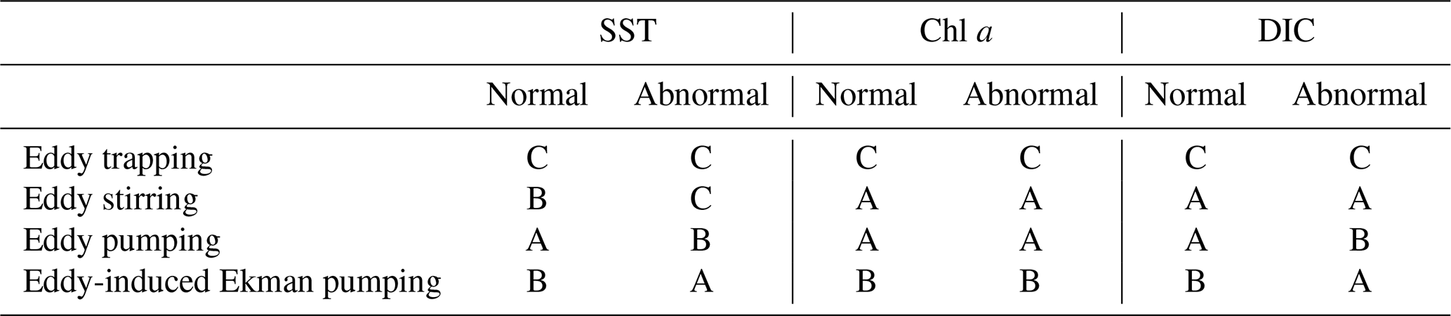
Section 5 reveals the distinct influence mechanisms of eddies on SST, Chl a, DIC, and pCO2, which vary based on the inherent properties of each parameter and the complex interactions between eddies and the biogeochemical processes in the SO. As shown in Table 1, we compare the significance magnitudes of different effects, including eddy trapping, stirring, pumping, and eddy-induced Ekman pumping, on SST, Chl a, and DIC. It should be noted that the seasonal modulation of the mixed layer is not discussed in our study due to the absence of significant seasonal variations in eddy-induced SST, Chl a, and DIC anomalies (Fig. S7). Additionally, the variability of pCO2 anomalies within eddies is controlled by the effects of SST, Chl a, and DIC; therefore, the eddy-driven mechanisms on pCO2 can be demonstrated by exploring the effects of eddies on SST, Chl a, and DIC.
Compared to SST, eddy stirring plays a more significant role in Chl a and DIC anomalies within eddies. As eddy stirring redistributes physical and biogeochemical parameters spatially through horizontal advection, the larger the horizontal parameter gradient, the stronger the eddy stirring effect (Mcgillicuddy, 2016). We calculate the average gradients of normalized SST, Chl a, and DIC in the SO from 1996 to 2015 and find their values are 0.05, 0.11, and 0.20, respectively. The specific method to obtain the gradients is demonstrated in Sect. S2 (Quarteroni et al., 2006). The small gradient of SST leads to a negligible effect of eddy stirring and results in more pronounced monopole patterns within eddies than other variables (Fig. 6a1–a4 and e1–e4).
By contrast, the average gradient of Chl a is nearly 2 times higher than that of SST; thus, eddy stirring can cause a stronger effect on Chl a. Both eddy stirring and eddy pumping contribute to the generation of negative/positive Chl a anomalies within AEs/CEs. The combined effects of eddy stirring and eddy pumping dominate the similar patterns of Chl a anomalies in normal and abnormal eddies. However, the effect of eddy-induced Ekman pumping on Chl a is relatively small and contributes to attenuating the magnitudes of Chl a anomalies within abnormal eddies (Fig. 6b1–b4 and f1–f4). The major limitation of marine Chl a is the insufficient supplement of nutrients from depth into the euphotic zone (Mahadevan, 2016). The transport of nutrients enriched in deep seawater is mainly controlled by eddy pumping. By contrast, the variations of SST and DIC anomalies are prone to be influenced by heat and carbon exchange at the ocean–atmosphere interface (Gaube et al., 2015; Song et al., 2016), making them susceptible to eddy-induced Ekman pumping. Consequently, Chl a anomalies in normal and abnormal eddies show similar patterns and signals, whereas SST and DIC anomalies in normal and abnormal eddies show opposite signals.
Such a limited influence of eddy-induced Ekman pumping on Chl a in the SO was also reported by Gaube et al. (2014), who plotted global maps of the cross-correlation of Chl a anomalies and SSH, as well as eddy-induced Ekman pumping, revealing a negative correlation between Chl a anomalies and SSH and a negative correlation between Chl a anomalies and eddy-induced Ekman pumping in most areas of the SO. These results indicate that AEs have negative Chl a anomalies and CEs have positive Chl a anomalies, and eddy-induced Ekman pumping does not dominate the variation of Chl a anomalies within eddies. In addition, we obtain the composite averages for Chl a anomalies in the BMC, defined by Gaube et al. (2014) as 305–330∘ E and 34–50∘ S (Fig. S8). The patterns are similar to those obtained by Gaube et al. (2014), with dominant monopole negative Chl a anomalies within AEs and positive Chl a anomalies within CEs. However, the magnitudes of Chl a anomalies within abnormal eddies are lower than normal eddies, which is related to the more pronounced impact of abnormal eddies in counteracting eddy pumping through the mechanism of Ekman pumping.
The average gradient of DIC is 4 times higher than that of SST, indicating that eddy stirring will have a more pronounced impact on DIC than on SST. As a result, the composite DIC anomalies within eddies show dipole patterns (Fig. 6c1–c4 and g1–g4). In addition to the different impacts of eddy stirring on SST and DIC, both eddy pumping and eddy-induced Ekman pumping contribute to the variations in these parameters (Table 1). In normal eddies, eddy pumping dominates the vertical distribution of SST and DIC. Within CCEs, the upwelling of cold, DIC-rich deep water induces negative SST anomalies and positive DIC anomalies, whereas the reverse is true for WAEs. However, the influence of eddy-induced Ekman pumping becomes more prominent within abnormal eddies. Within WCEs, the downwelling of warm, low-DIC surface waters induces positive SST anomalies and negative DIC anomalies, whereas the reverse is true for CAEs.
The impact of eddies on pCO2 anomalies varies by season and region, which arises from the combined effects of SST, Chl a, and DIC. In winter, the dominant DIC-driven effect leads to negative pCO2 anomalies in WAEs and WCEs and positive anomalies in CAEs and CCEs (Fig. 6d1–d4). However, in summer, the pCO2 anomalies are dominated by the combined effects of SST, Chl a, and DIC (Fig. 6h1–h4). Notably, the pCO2 anomalies within eddies are dominated by SST anomalies in the summer in SWA region, with smaller magnitudes of DIC anomalies (Fig. 9). In contrast, the pCO2 anomalies within eddies are dominated by DIC anomalies in the ARC, with larger magnitudes of DIC anomalies (Fig. 10).
In conclusion, using the eddy-centric composite method, we investigate the effects of normal and abnormal eddies on the variability of SST, Chl a, DIC, and pCO2 in the SO from 1996 to 2015. The distinct modifications in the physical and biogeochemical parameters of abnormal eddies compared to normal eddies stem from the effect of eddy-induced Ekman pumping. Figure S9 illustrates that in low-wind regions, specifically with wind speeds of less than 6 m s−1, the occurrence of abnormal eddies is scarce. Nevertheless, as wind speed progressively increases, the number of abnormal eddies generally increases. Considering that eddy-induced Ekman pumping is expected to exert a more pronounced influence in high-wind regions, this result indicates the effect of eddy-induced Ekman pumping on the generation of abnormal eddies. Specifically, in the SWA region dominated by abnormal eddies, the contributions of abnormal eddies to pCO2 are opposite to normal eddies and are about twice as high as normal eddies (Table S5). The current research commonly combines all the AEs or CEs and masks the presence of CAEs and WCEs with very different upper ocean properties. Given their abundance, considering the distinct role of abnormal eddies when investigating eddy-induced modulation in physical and biogeochemical parameters provides a more accurate estimation of the impact of mesoscale eddies.
The observational-based study of basin-wide surface physical and biogeochemical parameters within SO mesoscale eddies provides important insights into the SO ecosystem and carbon cycling. The spatial redistribution of Chl a concentrations through eddy stirring and eddy pumping indicates the potential for localized hotspots of productivity and nutrient supply within eddies. Moreover, the impacts of eddy pumping and eddy-induced Ekman pumping on DIC distributions highlight the role of eddies in transporting carbon-rich waters, which can significantly influence the regional carbon budget and oceanic carbon uptake. Understanding the complexity of eddy-driven processes in the SO is crucial for accurately simulating and predicting the biogeochemical dynamics of the SO and its role in the global carbon cycle. Further investigations focusing on the specific mechanisms driving the observed patterns and their consequences for larger-scale oceanic processes will provide valuable insights into the role of mesoscale eddies in the SO.
All data used in the analysis are available in public repositories. The OISST data are available from https://doi.org/10.25921/RE9P-PT57 (Huang et al., 2020). The Chl a product is available from https://data.marine.copernicus.eu/product/OCEANCOLOUR_GLO_BGC_L3_MY_009_103/services (Marine Data Store, 2023a). The pCO2 and DIC datasets are available from https://www.data.jma.go.jp/gmd/kaiyou/english/co2_flux/co2_flux_data_en.html (Iida et al., 2021). The normal and abnormal eddies datasets are available from https://figshare.com/s/3c3b03776d9862ac85bc (Liu et al., 2021) for peer review only. The CCMP vector wind data are available from https://doi.org/10.56236/RSS-uv6h30 (Mears et al., 2022). The AVISO altimeter current product is available from https://data.marine.copernicus.eu/product/SEALEVEL_GLO_PHY_L4_MY_008_047/services (Marine Data Store, 2023b). The positions of the main ACC fronts (Polar Front and Subantarctic Front) are available from http://ctoh.legos.obs-mip.fr/data/southern-ocean-fronts-extraction-form (Sallée et al., 2008).
The supplement related to this article is available online at: https://doi.org/10.5194/bg-20-4857-2023-supplement.
QL, YL, and XL conceived the project. QL did the writing and original draft preparation. All authors provided feedback on the analysis and interpretation of results and contributed to reviewing and editing the paper. All authors have read and agreed to the published version of the paper.
The contact author has declared that none of the authors has any competing interests.
Publisher’s note: Copernicus Publications remains neutral with regard to jurisdictional claims made in the text, published maps, institutional affiliations, or any other geographical representation in this paper. While Copernicus Publications makes every effort to include appropriate place names, the final responsibility lies with the authors.
This work was supported by the Qingdao National Laboratory for Marine Science and Technology, the special fund of Shandong Province (no. 2022QNLM050301-2), the Natural Science Foundation of Shandong Province (ZR2020MD083), the National Natural Science Foundation of China (U2006211 and 42306194), and the Strategic Priority Research Program of the Chinese Academy of Sciences (XDB42000000).
This research has been supported by the Qingdao National Laboratory for Marine Science and Technology, the special fund of Shandong Province (no. 2022QNLM050301-2), the Natural Science Foundation of Shandong Province (ZR2020MD083), the National Natural Science Foundation of China (U2006211 and 42306194), and the Strategic Priority Research Program of the Chinese Academy of Sciences (XDB42000000).
This paper was edited by Carolin Löscher and reviewed by Lydia Keppler and two anonymous referees.
Altabet, M. A., Ryabenko, E., Stramma, L., Wallace, D. W. R., Frank, M., Grasse, P., and Lavik, G.: An eddy-stimulated hotspot for fixed nitrogen-loss from the Peru oxygen minimum zone, Biogeosciences, 9, 4897–4908, https://doi.org/10.5194/bg-9-4897-2012, 2012.
Assassi, C., Morel, Y., Vandermeirsch, F., Chaigneau, A., Pegliasco, C., Morrow, R., Colas, F., Fleury, S., Carton, X., Klein, P., and Cambra, R.: An Index to Distinguish Surface- and Subsurface-Intensified Vortices from Surface Observations, J. Phys. Oceanogr., 46, 2529–2552, https://doi.org/10.1175/jpo-d-15-0122.1, 2016.
Bakker, D. C. E., Pfeil, B., Landa, C. S., Metzl, N., O'Brien, K. M., Olsen, A., Smith, K., Cosca, C., Harasawa, S., Jones, S. D., Nakaoka, S., Nojiri, Y., Schuster, U., Steinhoff, T., Sweeney, C., Takahashi, T., Tilbrook, B., Wada, C., Wanninkhof, R., Alin, S. R., Balestrini, C. F., Barbero, L., Bates, N. R., Bianchi, A. A., Bonou, F., Boutin, J., Bozec, Y., Burger, E. F., Cai, W.-J., Castle, R. D., Chen, L., Chierici, M., Currie, K., Evans, W., Featherstone, C., Feely, R. A., Fransson, A., Goyet, C., Greenwood, N., Gregor, L., Hankin, S., Hardman-Mountford, N. J., Harlay, J., Hauck, J., Hoppema, M., Humphreys, M. P., Hunt, C. W., Huss, B., Ibánhez, J. S. P., Johannessen, T., Keeling, R., Kitidis, V., Körtzinger, A., Kozyr, A., Krasakopoulou, E., Kuwata, A., Landschützer, P., Lauvset, S. K., Lefèvre, N., Lo Monaco, C., Manke, A., Mathis, J. T., Merlivat, L., Millero, F. J., Monteiro, P. M. S., Munro, D. R., Murata, A., Newberger, T., Omar, A. M., Ono, T., Paterson, K., Pearce, D., Pierrot, D., Robbins, L. L., Saito, S., Salisbury, J., Schlitzer, R., Schneider, B., Schweitzer, R., Sieger, R., Skjelvan, I., Sullivan, K. F., Sutherland, S. C., Sutton, A. J., Tadokoro, K., Telszewski, M., Tuma, M., van Heuven, S. M. A. C., Vandemark, D., Ward, B., Watson, A. J., and Xu, S.: A multi-decade record of high-quality fCO2 data in version 3 of the Surface Ocean CO2 Atlas (SOCAT), Earth Syst. Sci. Data, 8, 383–413, https://doi.org/10.5194/essd-8-383-2016, 2016.
Butterworth, S.: On the theory of filter amplifiers, Wireless Engineer 193–195, 1930.
Campbell, J. W.: The lognormal distribution as a model for bio-optical variability in the sea, J. Geophys. Res.-Oceans, 100, 13237–13254, https://doi.org/10.1029/95JC00458, 1995.
Castellani, M.: Identification of eddies from sea surface temperature maps with neural networks, Int. J. Remote Sens., 27, 1601–1618, https://doi.org/10.1080/01431160500462170, 2006.
Chelton, D. B., Schlax, M. G., and Samelson, R. M.: Global observations of nonlinear mesoscale eddies, Prog. Oceanogr., 91, 167–216, https://doi.org/10.1016/j.pocean.2011.01.002, 2011a.
Chelton, D. B., Gaube, P., Schlax, M. G., Early, J. J., and Samelson, R. M.: The Influence of Nonlinear Mesoscale Eddies on Near-Surface Oceanic Chlorophyll, Science, 334, 328–332, https://doi.org/10.1126/science.1208897, 2011b.
Chen, F., Cai, W.-J., Benitez-Nelson, C., and Wang, Y.: Sea surface pCO2-SST relationships across a cold-core cyclonic eddy: Implications for understanding regional variability and air-sea gas exchange, Geophys. Res. Lett., 34, 265–278, https://doi.org/10.1029/2006gl028058, 2007.
Cornec, M., Laxenaire, R., Speich, S., and Claustre, H.: Impact of Mesoscale Eddies on Deep Chlorophyll Maxima, Geophys. Res. Lett., 48, e2021GL093470, https://doi.org/10.1029/2021GL093470, 2021.
Cushman-Roisin, B. and Beckers, J.-M.: Chapter 18 – Fronts, Jets and Vortices, in: International Geophysics, edited by: Cushman-Roisin, B. and Beckers, J.-M., Academic Press, 589–623, https://doi.org/10.1016/B978-0-12-088759-0.00018-3, 2011.
Dawson, H. R. S., Strutton, P. G., and Gaube, P.: The Unusual Surface Chlorophyll Signatures of Southern Ocean Eddies, J. Geophys. Res.-Oceans, 123, 6053–6069, https://doi.org/10.1029/2017JC013628, 2018.
Denvil-Sommer, A., Gehlen, M., Vrac, M., and Mejia, C.: LSCE-FFNN-v1: a two-step neural network model for the reconstruction of surface ocean pCO2 over the global ocean, Geosci. Model Dev., 12, 2091–2105, https://doi.org/10.5194/gmd-12-2091-2019, 2019.
Dilmahamod, A. F., Aguiar-González, B., Penven, P., Reason, C. J. C., De Ruijter, W. P. M., Malan, N., and Hermes, J. C.: SIDDIES Corridor: A Major East-West Pathway of Long-Lived Surface and Subsurface Eddies Crossing the Subtropical South Indian Ocean, J. Geophys. Res.-Oceans, 123, 5406–5425, https://doi.org/10.1029/2018JC013828, 2018.
Dolz, J., Gopinath, K., Yuan, J., Lombaert, H., Desrosiers, C., and Ben Ayed, I.: HyperDense-Net: A Hyper-Densely Connected CNN for Multi-Modal Image Segmentation, IEEE Trans. Med. Imaging, 38, 1116–1126, https://doi.org/10.1109/TMI.2018.2878669, 2019.
Dong, C. M., McWilliams, J. C., Liu, Y., and Chen, D. K.: Global heat and salt transports by eddy movement, Nat. Commun., 5, 3294, https://doi.org/10.1038/ncomms4294, 2014.
Ducet, N., Le Traon, P. Y., and Reverdin, G.: Global high-resolution mapping of ocean circulation from TOPEX/Poseidon and ERS-1 and -2, J. Geophys. Res.-Oceans, 105, 19477–19498, https://doi.org/10.1029/2000JC900063, 2000.
Dufois, F., Hardman-Mountford, N. J., Greenwood, J., Richardson, A. J., Feng, M., Herbette, S., and Matear, R.: Impact of eddies on surface chlorophyll in the South Indian Ocean, J. Geophys. Res.-Oceans, 119, 8061–8077,https://doi.org/10.1002/2014JC010164, 2014.
Everett, J. D., Baird, M. E., Oke, P. R., and Suthers, I. M.: An avenue of eddies: Quantifying the biophysical properties of mesoscale eddies in the Tasman Sea, Geophys. Res. Lett., 39, L16608, https://doi.org/10.1029/2012gl053091, 2012.
Faghmous, J. H., Frenger, I., Yao, Y., Warmka, R., Lindell, A., and Kumar, V.: A daily global mesoscale ocean eddy dataset from satellite altimetry, Sci. Data, 2, 150028, https://doi.org/10.1038/sdata.2015.28, 2015.
Falk, T., Mai, D., Bensch, R., Cicek, O., Abdulkadir, A., Marrakchi, Y., Bohm, A., Deubner, J., Jackel, Z., Seiwald, K., Dovzhenko, A., Tietz, O., Dal Bosco, C., Walsh, S., Saltukoglu, D., Tay, T. L., Prinz, M., Palme, K., Simons, M., Diester, I., Brox, T., and Ronneberger, O.: U-Net: deep learning for cell counting, detection, and morphometry, Nat. Methods, 16, 67–70, https://doi.org/10.1038/s41592-018-0261-2, 2019.
Fay, A. R., Lovenduski, N. S., McKinley, G. A., Munro, D. R., Sweeney, C., Gray, A. R., Landschützer, P., Stephens, B. B., Takahashi, T., and Williams, N.: Utilizing the Drake Passage Time-series to understand variability and change in subpolar Southern Ocean pCO2, Biogeosciences, 15, 3841–3855, https://doi.org/10.5194/bg-15-3841-2018, 2018.
Frenger, I., Gruber, N., Knutti, R., and Münnich, M.: Imprint of Southern Ocean eddies on winds, clouds and rainfall, Nat. Geosci., 6, 608–612, https://doi.org/10.1038/ngeo1863, 2013.
Frenger, I., Münnich, M., Gruber, N., and Knutti, R.: Southern Ocean eddy phenomenology, J. Geophys. Res.-Oceans, 120, 7413–7449, https://doi.org/10.1002/2015jc011047, 2015.
Frenger, I., Münnich, M., and Gruber, N.: Imprint of Southern Ocean mesoscale eddies on chlorophyll, Biogeosciences, 15, 4781–4798, https://doi.org/10.5194/bg-15-4781-2018, 2018.
Garnesson, P., Mangin, A., Fanton d'Andon, O., Demaria, J., and Bretagnon, M.: The CMEMS GlobColour chlorophyll a product based on satellite observation: multi-sensor merging and flagging strategies, Ocean Sci., 15, 819–830, https://doi.org/10.5194/os-15-819-2019, 2019.
Gaube, P., Chelton, D. B., Strutton, P. G., and Behrenfeld, M. J.: Satellite observations of chlorophyll, phytoplankton biomass, and Ekman pumping in nonlinear mesoscale eddies, J. Geophys. Res.-Oceans, 118, 6349–6370, https://doi.org/10.1002/2013JC009027, 2013.
Gaube, P., McGillicuddy Jr., D. J., Chelton, D. B., Behrenfeld, M. J., and Strutton, P. G.: Regional variations in the influence of mesoscale eddies on near-surface chlorophyll, J. Geophys. Res.-Oceans, 119, 8195–8220, https://doi.org/10.1002/2014JC010111, 2014.
Gaube, P., Chelton, D. B., Samelson, R. M., Schlax, M. G., and O'Neill, L. W.: Satellite Observations of Mesoscale Eddy-Induced Ekman Pumping, J. Phys. Oceanogr., 45, 104–132, https://doi.org/10.1175/jpo-d-14-0032.1, 2015.
Gille, S. T., Carranza, M. M., Cambra, R., and Morrow, R.: Wind-induced upwelling in the Kerguelen Plateau region, Biogeosciences, 11, 6389–6400, https://doi.org/10.5194/bg-11-6389-2014, 2014.
Gohin, F., Druon, J. N., and Lampert, L.: A five channel chlorophyll concentration algorithm applied to SeaWiFS data processed by SeaDAS in coastal waters, Int. J. Remote Sens., 23, 1639–1661, https://doi.org/10.1080/01431160110071879, 2002.
Hashihama, F., Yasuda, I., Kumabe, A., Sato, M., Sasaoka, H., Iida, Y., Shiozaki, T., Saito, H., Kanda, J., Furuya, K., Boyd, P. W., and Ishii, M.: Nanomolar phosphate supply and its recycling drive net community production in the subtropical North Pacific, Nat. Commun., 12, 3462, https://doi.org/10.1038/s41467-021-23837-y, 2021.
Hausmann, U. and Czaja, A.: The observed signature of mesoscale eddies in sea surface temperature and the associated heat transport, Deep-Sea Res. Part I, 70, 60–72, https://doi.org/10.1016/j.dsr.2012.08.005, 2012.
Hu, C., Lee, Z., and Franz, B.: Chlorophyll aalgorithms for oligotrophic oceans: A novel approach based on three-band reflectance difference, J. Geophys. Res.-Oceans, 117, C01011, https://doi.org/10.1029/2011JC007395, 2012.
Huang, B., Liu, C., Banzon, V. F., Freeman, E., Graham, G., Hankins, W., Smith, T. M., and Zhang, H.-M.: NOAA 0.25-degree Daily Optimum Interpolation Sea Surface Temperature (OISST), Version 2.1, NOAA National Centers for Environmental Information [data set], https://doi.org/10.25921/RE9P-PT57, 2020.
Huang, J., Xu, F., Zhou, K., Xiu, P., and Lin, Y.: Temporal evolution of near-surface chlorophyll over cyclonic eddy lifecycles in the southeastern Pacific, J. Geophys. Res.-Oceans, 122, 6165–6179, https://doi.org/10.1002/2017JC012915, 2017.
Iida, Y., Takatani, Y., Kojima, A., and Ishii, M.: Global trends of ocean CO2 sink and ocean acidification: an observation-based reconstruction of surface ocean inorganic carbon variables, J. Oceanogr., 77, 323–358, https://doi.org/10.1007/s10872-020-00571-5, 2021.
Jersild, A. and Ito, T.: Physical and Biological Controls of the Drake Passage pCO2 Variability, Global Biogeochem. Cy., 34, e2020GB006644, https://doi.org/10.1029/2020gb006644, 2020.
Jiang, C., Gille, S. T., Sprintall, J., and Sweeney, C.: Drake Passage Oceanic pCO2: Evaluating CMIP5 Coupled Carbon–Climate Models Using in situ Observations, J. Climate, 27, 76–100, https://doi.org/10.1175/jcli-d-12-00571.1, 2014.
Jones, E. M., Hoppema, M., Strass, V., Hauck, J., Salt, L., Ossebaar, S., Klaas, C., van Heuven, S. M. A. C., Wolf-Gladrow, D., Stöven, T., and de Baar, H. J. W.: Mesoscale features create hotspots of carbon uptake in the Antarctic Circumpolar Current, Deep Sea Res. Part II, 138, 39–51, https://doi.org/10.1016/j.dsr2.2015.10.006, 2017.
Landschützer, P., Gruber, N., Bakker, D. C. E., and Schuster, U.: Recent variability of the global ocean carbon sink, Global Biogeochem. Cy., 28, 927–949, https://doi.org/10.1002/2014gb004853, 2014.
Landschützer, P., Gruber, N., Haumann, F. A., Rödenbeck, C., Bakker, D. C. E., Heuven, S. v., Hoppema, M., Metzl, N., Sweeney, C., Takahashi, T., Tilbrook, B., and Wanninkhof, R.: The reinvigoration of the Southern Ocean carbon sink, Science, 349, 1221–1224, https://doi.org/10.1126/science.aab2620, 2015.
Lasternas, S., Piedeleu, M., Sangrà, P., Duarte, C. M., and Agustí, S.: Forcing of dissolved organic carbon release by phytoplankton by anticyclonic mesoscale eddies in the subtropical NE Atlantic Ocean, Biogeosciences, 10, 2129–2143, https://doi.org/10.5194/bg-10-2129-2013, 2013.
Le Quéré, C., Rödenbeck, C., Buitenhuis, E. T., Conway, T. J., Langenfelds, R., Gomez, A., Labuschagne, C., Ramonet, M., Nakazawa, T., Metzl, N., Gillett, N., and Heimann, M.: Saturation of the Southern Ocean CO2 Sink Due to Recent Climate Change, Science, 316, 1735–1738, https://doi.org/10.1126/science.1136188, 2007.
Leyba, I. M., Saraceno, M., and Solman, S. A.: Air-sea heat fluxes associated to mesoscale eddies in the Southwestern Atlantic Ocean and their dependence on different regional conditions, Clim. Dynam., 49, 2491–2501, https://doi.org/10.1007/s00382-016-3460-5, 2017.
Liu, Y., Chen, G., Sun, M., Liu, S., and Tian, F.: A Parallel SLA-Based Algorithm for Global Mesoscale Eddy Identification, J. Atmos. Ocean. Technol., 33, 2743–2754, https://doi.org/10.1175/JTECH-D-16-0033.1, 2016.
Liu, Y., Yu, L., and Chen, G.: Characterization of Sea Surface Temperature and Air-Sea Heat Flux Anomalies Associated With Mesoscale Eddies in the South China Sea, J. Geophys. Res.-Oceans, 125, e2019JC015470, https://doi.org/10.1029/2019jc015470, 2020.
Liu, Y., Zheng, Q., and Li, X.: Characteristics of Global Ocean Abnormal Mesoscale Eddies Derived From the Fusion of Sea Surface Height and Temperature Data by Deep Learning, Geophys. Res. Lett., 48, e2021GL094772, https://doi.org/10.1029/2021gl094772, 2021.
Mahadevan, A.: The Impact of Submesoscale Physics on Primary Productivity of Plankton, Annu. Rev. Mar. Science, 8, 161–184, https://doi.org/10.1146/annurev-marine-010814-015912, 2016.
Marine Data Store (MDS): Global Ocean Colour (Copernicus-GlobColour), Bio-Geo-Chemical, L3 (daily) from Satellite Observations (1997–ongoing), E.U. Copernicus Marine Service Information (CMEMS) [data set], https://doi.org/10.48670/moi-00280, 2023a.
Marine Data Store (MDS): Global Ocean Gridded L 4 Sea Surface Heights And Derived Variables Reprocessed 1993 Ongoing, E.U. Copernicus Marine Service Information (CMEMS), https://doi.org/10.48670/moi-00148, 2023b.
Marshall, J. and Speer, K.: Closure of the meridional overturning circulation through Southern Ocean upwelling, Nat. Geosci., 5, 171–180, https://doi.org/10.1038/ngeo1391, 2012.
Mathis, J. T., Pickart, R. S., Hansell, D. A., Kadko, D., and Bates, N. R.: Eddy transport of organic carbon and nutrients from the Chukchi Shelf: Impact on the upper halocline of the western Arctic Ocean, J. Geophys. Res.-Oceans, 112, C05011, https://doi.org/10.1029/2006jc003899, 2007.
McGillicuddy, D. J.: Formation of Intrathermocline Lenses by Eddy–Wind Interaction, J. Phys. Oceanogr., 45, 606–612, https://doi.org/10.1175/jpo-d-14-0221.1, 2015.
McGillicuddy, D. J.: Mechanisms of Physical-Biological-Biogeochemical Interaction at the Oceanic Mesoscale, Annu. Rev. Mar. Science, 8, 125–159, https://doi.org/10.1146/annurev-marine-010814-015606, 2016.
McGillicuddy, D. J. and Robinson, A. R.: Eddy-induced nutrient supply and new production in the Sargasso Sea, Deep Sea Res. Part I, 44, 1427–1450, https://doi.org/10.1016/S0967-0637(97)00024-1, 1997.
McGillicuddy, D. J., Robinson, A. R., Siegel, D. A., Jannasch, H. W., Johnson, R., Dickey, T. D., McNeil, J., Michaels, A. F., and Knap, A. H.: Influence of mesoscale eddies on new production in the Sargasso Sea, Nature, 394, 263–266, https://doi.org/10.1038/28367, 1998.
McGillicuddy, D. J., Anderson, L. A., Bates, N. R., Bibby, T., Buesseler, K. O., Carlson, C. A., Davis, C. S., Ewart, C., Falkowski, P. G., Goldthwait, S. A., Hansell, D. A., Jenkins, W. J., Johnson, R., Kosnyrev, V. K., Ledwell, J. R., Li, Q. P., Siegel, D. A., and Steinberg, D. K.: Eddy/Wind Interactions Stimulate Extraordinary Mid-Ocean Plankton Blooms, Science, 316, 1021–1026, https://doi.org/10.1126/science.1136256, 2007.
Mears, C., Lee, T., Ricciardulli, L., Wang, X., and Wentz, F.: RSS Cross-Calibrated Multi-Platform (CCMP) 6-hourly ocean vector wind analysis on 0.25 deg grid, Version 3.0, Remote Sensing Systems [data set], Santa Rosa, CA, https://doi.org/10.56236/RSS-uv6h30, 2022.
Melnichenko, O., Amores, A., Maximenko, N., Hacker, P., and Potemra, J.: Signature of mesoscale eddies in satellite sea surface salinity data, J. Geophys. Res.-Oceans, 122, 1416–1424, https://doi.org/10.1002/2016jc012420, 2017.
Munro, D. R., Lovenduski, N. S., Stephens, B. B., Newberger, T., Arrigo, K. R., Takahashi, T., Quay, P. D., Sprintall, J., Freeman, N. M., and Sweeney, C.: Estimates of net community production in the Southern Ocean determined from time series observations (2002–2011) of nutrients, dissolved inorganic carbon, and surface ocean pCO2 in Drake Passage, Deep Sea Res. Part II, 114, 49–63, https://doi.org/10.1016/j.dsr2.2014.12.014, 2015.
Nencioli, F., Chang, G., Twardowski, M., and Dickey, T. D.: Optical Characterization of an Eddy-induced Diatom Bloom West of the Island of Hawaii, Biogeosciences, 7, 151–162, https://doi.org/10.5194/bg-7-151-2010, 2010.
Ni, Q., Zhai, X., Jiang, X., and Chen, D.: Abundant Cold Anticyclonic Eddies and Warm Cyclonic Eddies in the Global Ocean, J. Phys. Oceanogr., 51, 2793–2806, https://doi.org/10.1175/jpo-d-21-0010.1, 2021.
Olsen, A., Lange, N., Key, R. M., Tanhua, T., Álvarez, M., Becker, S., Bittig, H. C., Carter, B. R., Cotrim da Cunha, L., Feely, R. A., van Heuven, S., Hoppema, M., Ishii, M., Jeansson, E., Jones, S. D., Jutterström, S., Karlsen, M. K., Kozyr, A., Lauvset, S. K., Lo Monaco, C., Murata, A., Pérez, F. F., Pfeil, B., Schirnick, C., Steinfeldt, R., Suzuki, T., Telszewski, M., Tilbrook, B., Velo, A., and Wanninkhof, R.: GLODAPv2.2019 – an update of GLODAPv2, Earth Syst. Sci. Data, 11, 1437–1461, https://doi.org/10.5194/essd-11-1437-2019, 2019.
Ono, H., Toyama, K., Enyo, K., Iida, Y., Sasano, D., Nakaoka, S.-I., and Ishii, M.: Meridional Variability in Multi-Decadal Trends of Dissolved Inorganic Carbon in Surface Seawater of the Western North Pacific Along the 165∘ E Line, J. Geophys. Res.-Oceans, 128, e2022JC018842, https://doi.org/10.1029/2022JC018842, 2023.
Pegliasco, C., Delepoulle, A., Mason, E., Morrow, R., Faugère, Y., and Dibarboure, G.: META3.1exp: a new global mesoscale eddy trajectory atlas derived from altimetry, Earth Syst. Sci. Data, 14, 1087–1107, https://doi.org/10.5194/essd-14-1087-2022, 2022.
Pickart, R. S., Weingartner, T. J., Pratt, L. J., Zimmermann, S., and Torres, D. J.: Flow of winter-transformed Pacific water into the Western Arctic, Deep Sea Res. Part II, 52, 3175–3198, https://doi.org/10.1016/j.dsr2.2005.10.009, 2005.
Qiu, S., Feng, Y., Zhang, Y., Qi, D., Wu, Y., and Du, Y.: A Surface pCO2 Increasing Hiatus in the Equatorial Pacific Ocean Since 2010, Geophys. Res. Lett., 48, e2021GL093612, https://doi.org/10.1029/2021GL093612, 2021.
Quarteroni, A., Sacco, R., and Saleri, F.: Numerical Mathematics (Texts in Applied Mathematics), Springer-Verlag, 2006.
Racapé, V., Monaco, L., Metzl, N., and Pierre, C.: Summer and winter distribution of ä13CDIC in surface waters of the South Indian Ocean [20∘S–60∘S], Tellus B: Chem. Phys. Meteorol., 62, 660–673, https://doi.org/10.1111/j.1600-0889.2010.00504.x, 2010.
Reichstein, M., Camps-Valls, G., Stevens, B., Jung, M., Denzler, J., Carvalhais, N., and Prabhat: Deep learning and process understanding for data-driven Earth system science, Nature, 566, 195–204, https://doi.org/10.1038/s41586-019-0912-1, 2019.
Reynolds, R. W., Smith, T. M., Liu, C., Chelton, D. B., Casey, K. S., and Schlax, M. G.: Daily High-Resolution-Blended Analyses for Sea Surface Temperature, J. Climate, 20, 5473–5496, https://doi.org/10.1175/2007jcli1824.1, 2007.
Ronneberger, O., Fischer, P., and Brox, T.: U-Net: Convolutional Networks for Biomedical Image Segmentation, Medical Image Computing and Computer-Assisted Intervention – MICCAI 2015, 234–241, https://doi.org/10.48550/arXiv.1505.04597, 2015.
Sallée, J. B., Speer, K., and Morrow, R.: Response of the Antarctic Circumpolar Current to Atmospheric Variability, J. Climate, 21, 3020–3039, https://doi.org/10.1175/2007JCLI1702.1, 2008.
Shimizu, Y., Yasuda, I., and Ito, S.-i.: Distribution and Circulation of the Coastal Oyashio Intrusion, J. Phys. Oceanogr., 31, 1561–1578, https://doi.org/10.1175/1520-0485(2001)031<1561:Dacotc>2.0.Co;2, 2001.
Siegel, D. A., Peterson, P., McGillicuddy Jr., D. J., Maritorena, S., and Nelson, N. B.: Bio-optical footprints created by mesoscale eddies in the Sargasso Sea, Geophys. Res. Lett., 38, L13608, https://doi.org/10.1029/2011GL047660, 2011.
Song, H., Marshall, J., Munro, D. R., Dutkiewicz, S., Sweeney, C., McGillicuddy, D. J., and Hausmann, U.: Mesoscale modulation of air-sea CO2 flux in Drake Passage, J. Geophys. Res.-Oceans, 121, 6635–6649, https://doi.org/10.1002/2016jc011714, 2016.
Stearns, S. D. and Ahmed, N.: Digital Signal Analysis, IEEE Transactions on Systems, Man, and Cybernetics, SMC-6, 724–724, https://doi.org/10.1109/TSMC.1976.4309433, 1976.
Stern, M. E.: Interaction of a uniform wind stress with a geostrophic vortex, Deep Sea Res. Oceanogr. Abstracts, 12, 355–367, https://doi.org/10.1016/0011-7471(65)90007-0, 1965.
Stramma, L., Bange, H. W., Czeschel, R., Lorenzo, A., and Frank, M.: On the role of mesoscale eddies for the biological productivity and biogeochemistry in the eastern tropical Pacific Ocean off Peru, Biogeosciences, 10, 7293–7306, https://doi.org/10.5194/bg-10-7293-2013, 2013.
Sun, W., Dong, C., Tan, W., and He, Y.: Statistical Characteristics of Cyclonic Warm-Core Eddies and Anticyclonic Cold-Core Eddies in the North Pacific Based on Remote Sensing Data, Remote Sens., 11, 208, https://doi.org/10.3390/rs11020208, 2019.
Villas Bôas, A. B., Sato, O. T., Chaigneau, A., and Castelão, G. P.: The signature of mesoscale eddies on the air-sea turbulent heat fluxes in the South Atlantic Ocean, Geophys. Res. Lett., 42, 1856–1862, https://doi.org/10.1002/2015gl063105, 2015.
Wang, Z., Bovik, A. C., Sheikh, H. R., and Simoncelli, E. P.: Image quality assessment: from error visibility to structural similarity, IEEE Trans. Image Process., 13, 600–612, https://doi.org/10.1109/TIP.2003.819861, 2004.
Xu, G., Dong, C., Liu, Y., Gaube, P., and Yang, J.: Chlorophyll Rings around Ocean Eddies in the North Pacific, Sci. Rep., 9, 2056, https://doi.org/10.1038/s41598-018-38457-8, 2019.
- Abstract
- Introduction
- Data
- Eddy analysis methodology
- Results
- Modulation mechanisms of normal and abnormal eddies to physical and biogeochemical parameters
- Discussion and conclusions
- Data availability
- Author contributions
- Competing interests
- Disclaimer
- Acknowledgements
- Financial support
- Review statement
- References
- Supplement