the Creative Commons Attribution 4.0 License.
the Creative Commons Attribution 4.0 License.
 | 03 Feb 2023
Meteorological responses of carbon dioxide and methane fluxes in the terrestrial and aquatic ecosystems of a subarctic landscape
Lauri Heiskanen
Juha-Pekka Tuovinen
Henriikka Vekuri
Aleksi Räsänen
Tarmo Virtanen
Sari Juutinen
Annalea Lohila
Juha Mikola
Mika Aurela
The subarctic landscape consists of a mosaic of forest, peatland, and aquatic ecosystems and their ecotones. The carbon (C) exchange between ecosystems and the atmosphere through carbon dioxide (CO2) and methane (CH4) fluxes varies spatially and temporally among these ecosystems. Our study area in Kaamanen in northern Finland covered 7 km2 of boreal subarctic landscape with upland forest, open peatland, pine bogs, and lakes. We measured the CO2 and CH4 fluxes with eddy covariance and chambers between June 2017 and June 2019 and studied the C flux responses to varying meteorological conditions. The landscape area was an annual CO2 sink of −45 ± 22 and −33 ± 23 g C m−2 and a CH4 source of 3.0 ± 0.2 and 2.7 ± 0.2 g C m−2 during the first and second study years, respectively. The pine forest had the largest contribution to the landscape-level CO2 sink, −126 ± 21 and −101 ± 19 g C m−2, and the fen to the CH4 emissions, 7.8 ± 0.2 and 6.3 ± 0.3 g C m−2, during the first and second study years, respectively. The lakes within the area acted as CO2 and CH4 sources to the atmosphere throughout the measurement period, and a lake located downstream from the fen with organic sediment showed 4-fold fluxes compared to a mineral sediment lake. The annual C balances were affected most by the rainy peak growing season in 2017, the warm summer in 2018, and a heatwave and drought event in July 2018. The rainy period increased ecosystem respiration (ER) in the pine forest due to continuously high soil moisture content, and ER was on a level similar to the following, notably warmer, summer. A corresponding ER response to abundant precipitation was not observed for the fen ecosystem, which is adapted to high water table levels, and thus a higher ER sum was observed during the warm summer 2018. During the heatwave and drought period, similar responses were observed for all terrestrial ecosystems, with decreased gross primary productivity and net CO2 uptake, caused by the unfavourable growing conditions and plant stress due to the soil moisture and vapour pressure deficits. Additionally, the CH4 emissions from the fen decreased during and after the drought. However, the timing and duration of drought effects varied between the fen and forest ecosystems, as C fluxes were affected sooner and had a shorter post-drought recovery time in the fen than forest. The differing CO2 flux response to weather variations showed that terrestrial ecosystems can have a contrasting impact on the landscape-level C balance in a changing climate, even if they function similarly most of the time.
- Article
(5097 KB) - Full-text XML
-
Supplement
(620 KB) - BibTeX
- EndNote


A typical boreal subarctic landscape consists of a mosaic of land cover types including forests, open and forested peatlands, and waterbodies, with each ecosystem acting as a source or sink of atmospheric carbon (C), depending on its characteristics and weather conditions. To grasp a full picture of the C balance at the landscape scale, the carbon dioxide (CO2) and methane (CH4) exchange between the main ecosystems and the atmosphere needs to be assessed. This is also because part of the C fixed in terrestrial systems can be emitted back to the atmosphere via aquatic ecosystems or transported out from the catchment. The net atmosphere–ecosystem CO2 exchange is a result of gross primary production (GPP) of plants and ecosystem respiration (ER), which is composed of autotrophic and heterotrophic respiration (Chapin et al., 2011). The CH4 emissions from ecosystems are mainly produced by methanogens in the waterlogged, anoxic zone in soils, while the CH4 uptake is caused by oxidation by methanotrophs in aerobic soil conditions (Le Mer and Roger, 2001).
As a result of the ongoing climate change, the subarctic regions warm rapidly, 2 to 3 times as fast as the rest of the world (Masson-Delmotte et al., 2018). The higher temperatures affect the C cycle of subarctic ecosystems by lengthening the growing season and shortening the snow and ice cover periods. Higher temperatures and a longer growing season enable greater CO2 uptake through photosynthesis (Aurela et al., 2004; Silfver et al., 2020), but they also allow greater CO2 emissions due to the increased heterotrophic and autotrophic respiration (Kätterer et al., 1998). However, the variation in ecosystem C dynamics is also highly dependent on water balance, as too low a moisture content in soils decreases the GPP and decomposition of organic matter (Jones, 2013; Meyer et al., 2018), and methanogenesis requires anoxic soil conditions (Chapin et al., 2011). In aquatic ecosystems, the longer ice-free periods, with increased C input from surrounding terrestrial ecosystems, lead to higher annual C emissions to the atmosphere (Cole et al., 2007; Guo et al., 2020). In a longer than 1-year time span, the effects of climate change are observed as vegetation composition shifts, such as Arctic shrubification that enhances CO2 uptake and alters ecosystem respiration and nutrient availability (Mekonnen et al., 2021). Concurrently, the potential of severe weather events, such as heatwaves and droughts, to affect the C cycle increases within the region (Masson-Delmotte et al., 2018).
Boreal upland forests have been shown to act as either annual net sinks or sources of atmospheric CO2, depending on species composition, climatic conditions, and the occurrence of extreme weather events, fires, and herbivores and pathogens (Bond-Lamberty et al., 2007; Kljun et al., 2007; Lindroth et al., 2008; Aurela et al., 2015; Hadden and Grelle, 2017), and these ecosystems usually act as small CH4 sinks (Dinsmore et al., 2017). Undrained boreal peatlands have been, in the long term, net CO2 sinks via the accumulation of organic C, but, similar to forests, their annual CO2 balance is sensitive to environmental conditions (Bubier et al., 1998; Aurela et al., 2004; Lindroth et al., 2007). Additionally, these peatlands release CH4 into the atmosphere (Chapin et al., 2011). Peatlands have more C stored in the soil but less C in living plant matter compared to upland forests, and thus, the same disturbances on the ecosystems can lead to differing effects on the C balance.
Globally, inland waters act as net CO2 and CH4 sources to the atmosphere (Tranvik et al., 2009). Boreal lakes vary greatly in their area and depth, input of organic and inorganic C from the terrestrial ecosystems, ice-free period duration, and the amount of C in sediments and aquatic vegetation, which all affect the magnitude of the C exchange with the atmosphere (Bastviken et al., 2004; Wik et al., 2018; Denfeld et al., 2020). Additionally, waterbodies provide paths for the lateral flow of water, C, and other matter between ecosystems (Cole et al., 2007).
The landscape-level C balance comprised of diverse ecosystems is evidently dependent on the ecosystem composition, and the regional effect of an environmental change or disturbance depends on the integrated response of individual ecosystems. As an example of such a disturbance, a heatwave and drought event encompassed northwestern Europe during the summer of 2018 (Lehtonen and Pirinen, 2019a, b). The drought conditions had different effects on the CO2 exchange of boreal forests and peatlands in the area (Rinne et al., 2020; Lindroth et al., 2020; Matkala et al., 2021). There was a large variation in how different forests reacted to the heatwave and drought, with some showing a substantial decrease and some no change or even an increase in CO2 uptake (Lindroth et al., 2020; Matkala et al., 2021). Most of the studied peatlands turned momentarily into CO2 sources during the drought, which lowered their annual CO2 uptake significantly and, simultaneously, the CH4 emissions decreased (Rinne et al., 2020). Thus, the landscape-level C balance depends on multiple responses, whose net effects are not easily predictable.
In this study, we assess the ecosystem–atmosphere exchange of CO2 and CH4 within a subarctic landscape based on eddy covariance and chamber measurements. The studied area in Kaamanen in northern Finland includes an upland pine forest, pine bogs, a mesotrophic flark fen, and shallow lakes of glacial origin. We focus on the temporal variation in C exchange during 2 full years (June 2017–June 2019). The meteorological conditions during the first year were similar to the long-term average, with the exception of the higher-than-average precipitation sum in summer. The second year included the above-mentioned heatwave and drought period. Motivated by the plant community-level study of Heiskanen et al. (2021), who found that the diversity of plant communities constrained C loss from the Kaamanen fen during the 2018 drought, we study if a similar pattern can be observed at the ecosystem level.

Figure 1The study area in Kaamanen with land cover type classification and flux measurement site locations.
Here, we address questions on how sensitive the C fluxes of different ecosystems are to changes in environmental conditions and how this is reflected on the landscape-level C exchange. The more specific scientific questions addressed are as follows: (1) what are the contributions of each ecosystem to the landscape-level CO2 and CH4 fluxes? (2) Do the CO2 and CH4 fluxes of different ecosystems show similar responses to varying meteorological conditions?
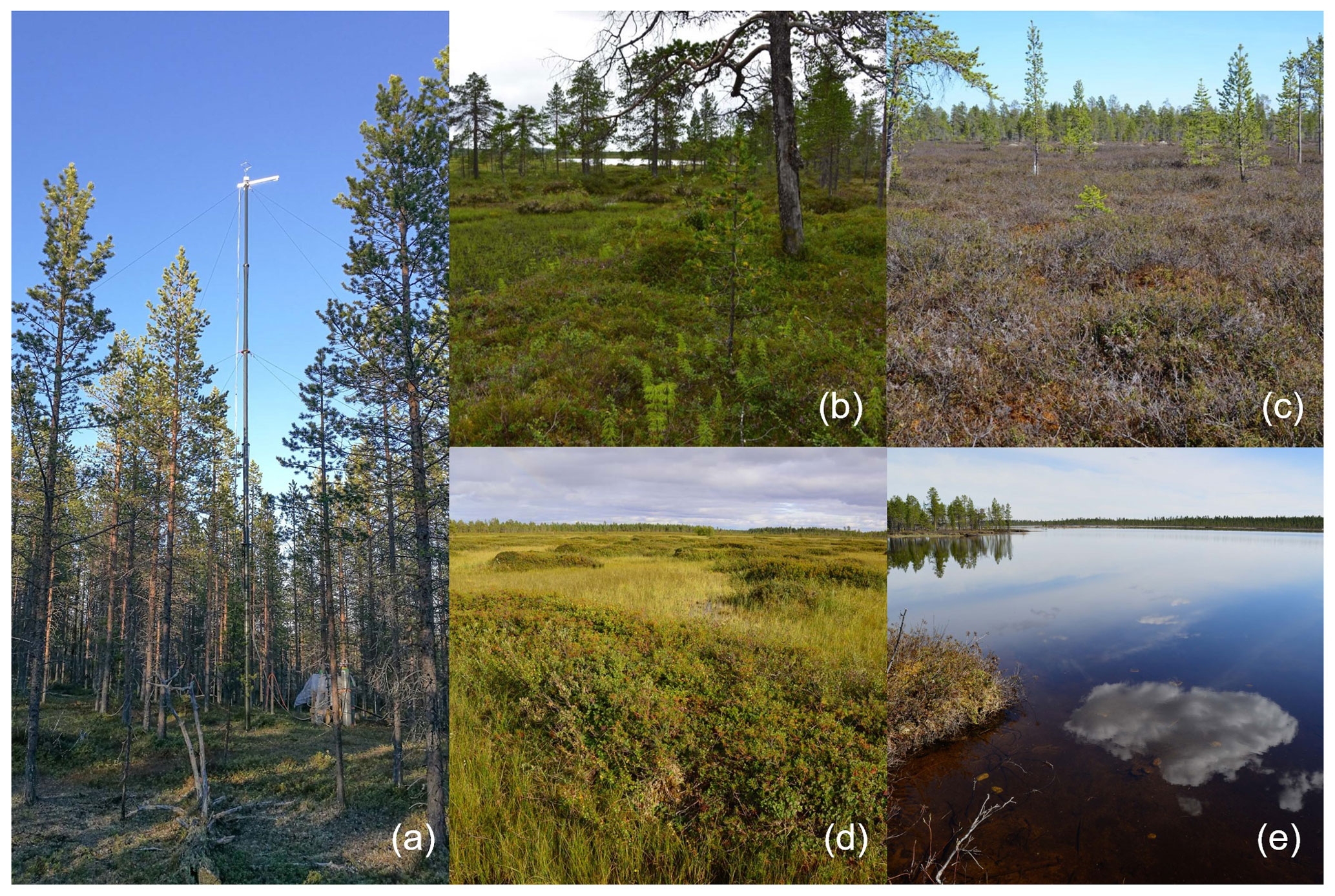
Figure 2The main ecosystem types within the study area are a (a) Scots pine forest, (b) treed pine bog, (c) sparsely treed pine bog, (d) fen, and (e) lake. Photo credits: (a) Lauri Heiskanen and (b–e) Tarmo Virtanen.
2.1 Study site
The studied landscape is located in Kaamanen in northern Finland (69∘8′ N, 27∘16′ E; 155 – above sea level ) within the subarctic climate zone and the northern boreal vegetation zone. The annual mean temperature in the region was −0.4 ∘C and the mean annual precipitation sum 472 mm in 1981–2010 (Pirinen et al., 2012). Even though the study area is located within the sporadic permafrost zone, no permafrost has been found there anymore in recent decades (Fronzek et al., 2010). The growing season is short and lasts for 150–180 d (Aurela et al., 2002). The study area covers 7 km2 around the flux measurement sites (Fig. 1) and consists of five main ecosystem types, namely an upland pine forest, a patterned mesotrophic flark fen, a treed pine bog, a sparsely treed pine bog, and lakes and a connecting stream (Fig. 2). The ecosystems within the study area are homogeneous in their species composition and provide a representative sample of the landscape.
Table 1Relative areal coverage of the land cover types within the study area.
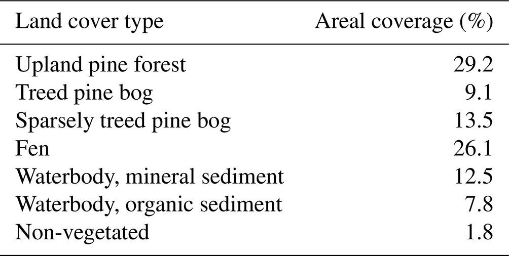
The areal coverage of different ecosystem types in the landscape was estimated with a land cover classification utilising remote sensing data and field observations, following the methodology described by Räsänen and Virtanen (2019). An aerial orthophoto was segmented, and 55 features for each segment were calculated from multi-source remote sensing data, including orthophoto, aerial laser scanning, and satellite imagery, and a supervised random forest classification (Breiman, 2001) was carried out using field data for model training and validation (Sect. S1 in the Supplement). The pine forest, pine bog, fen, and lake ecosystems each encompass roughly an equal area (Table 1). The ecosystems in the area are pristine with the exception of some forest logging, thinning, and selective removal of birches in part of the pine-dominated forests.
The mesotrophic patterned flark fen is an open peatland ecosystem characterised by a mosaic of string and flark microforms. The string formations are 0.5–1 m high and can remain frozen until the late summer (Aurela et al., 2001). The fen vegetation has also a clear patterning and can be partitioned to five distinct plant community types (PCTs) that differ in their vegetation composition, water table level, and carbon fluxes such as flark, Trichophorum tussock, string margin, string top, and tall sedge fen (Maanavilja et al., 2011; Räsänen et al., 2019; Heiskanen et al., 2021). In the flarks, the plant communities are dominated by sedges, including Trichophorum tussocks, and brown mosses. The top of the strings act as ombrotrophic bog-like surfaces within the fen and are covered mainly by dwarf shrubs, herbs, mosses, and lichens, while string margins are populated by dwarf birch (Betula nana) and other dwarf shrubs, sedges, and Sphagnum mosses. The fifth PCT, a tall sedge fen that is covered by tall sedges, deciduous shrubs, and forbs, can be found in the riparian areas of lakes and small streams. The species composition of these PCTs was described in detail by Maanavilja et al. (2011) and Räsänen et al. (2019) and in the paleorecords by Piilo et al. (2020). The bedrock under the peatland slopes towards the south. The average peat thickness increases from 1 m in the northern part of the fen towards the south, where it is up to 4 m (Piilo et al., 2020). Most of the aboveground biomass of the peatland resides in shrubs and mosses, and forbs and graminoids contribute increasingly to the total leaf area in the mid- and late growing season (Table A1 in the Appendix).
The dominant tree species in the upland mineral soil forest is Scots pine (Pinus sylvestris), with a few downy birch (Betula pubescens) trees also present (Table A2). The forest around the flux measurement site was logged about 50 years ago, but most of the pine forests within the study area are pine-dominated old-growth forest with an uneven age distribution. The average heights of all trees and the main canopy were approximately 8 and 11 m, respectively (Table A3). The field layer is dominated by evergreen dwarf shrubs (e.g. Vaccinium vitis-idaea and Calluna vulgaris), and the ground layer is covered by mosses and lichens. The soil type in the forest is sandy podzol, which has higher bulk density, lower nitrogen (N) content, and higher C : N ratio than the soil in the peatlands (Table A4; Sect. S2). Mosses and lichens contribute about 10 % to the total aboveground biomass (Tables A1 and A5).
The tree height and density decrease from the upland pine forest to the pine bog ecosystems. The average tree height in the pine bog was 5 m, and in the treed pine bog and sparsely treed pine bog, the aboveground tree biomass was about 50 % and 16 %, respectively, of the biomass in the pine forest (Tables A3 and A5). The field layer vegetation of the pine bog ecosystems is similar to that of the string tops (Table A1), with evergreen (Ledum palustre) and deciduous (Vaccinium uliginosum and Betula nana) shrubs, herbs (Rubus chamaemorus), and graminoids (mostly Carex spp.). The pine bog ground layer is formed by mosses and a few lichens. The soil carbon content is higher in the sparsely treed bog patches within the fen than in bog vegetation with thinner organic layer at the forest edge. Soil N content and C:N ratio are similar to those found in pine forest and string tops (Table A4).
The waterbodies within the study area vary in size from small streams and ponds to lakes larger than 25 ha (Lake Ulkujärvi in the northwest and Lake Jänkäjärvi in the south; Fig. 1). The lakes in the area are shallow, with the depth ranging from less than 1 m to a few metres, and have a sandy or organic sediment bottom. Most waterbodies in the study area belong to the same catchment, with water flowing from north to south. The aquatic vegetation is sparse, consisting of macrophytes, mainly horsetail (Equisetum fluviatile), sedges (Carex spp.), Menyanthes trifoliata, and benthic algae, near the shore. A few-metres-wide stream flows through the peatland and connects Lake Ulkujärvi to Lake Jänkäjärvi. Additionally, water flows on the surface across the fen and through the peat layers and eskers. Each year, during the spring thaw, the fen and part of the pine bogs become flooded.
2.2 Flux measurement methods
2.2.1 Pine forest CO2 flux measurements
The CO2 flux measurements in the Scots pine forest were set up at the beginning of the growing season in 2017, and the data acquisition was started on 8 June 2017. The eddy covariance (EC) measurements were conducted on a 14 m tall tower that was located on the southern edge of the forest so that, in the wind sector 250–65∘, the forest coverage was higher than 80 %. The EC system consisted of a three-axis sonic anemometer (USA-1; METEK Meteorologische Messtechnik GmbH, Germany) and a closed-path infrared gas analyser for CO2 and H2O mixing ratios (LI-7200; LI-COR Biosciences, USA). The inlet tube for the gas analyser was ∼ 18 m long and had an inner tube diameter of 3.1 mm. The flow rate was 5–6 L min−1.
The sampling frequency for the EC flux data was 10 Hz. Standard methods were used for calculating the half-hourly turbulent fluxes (Aubinet et al., 2012), with block averaging and a double rotation of the coordinate system (McMillen, 1988). The high-frequency signal attenuation flux losses were taken into account using an experimental transfer function with a half-power frequency of 1.9 Hz (Laurila et al., 2005).
The half-hourly averaged data were accepted based on the following screening criteria: relative stationarity < 100 % (Foken and Wichura, 1996), amount of recorded data per 30 min > 17 400, number of signal spikes per 30 min < 360, and mean CO2 mixing ratio within 340–550 ppm (parts per million). A friction velocity (u∗) limit of 0.24 m s−1 was used for screening the periods of insufficient turbulence. Data from the wind direction sector 250–65∘ were used to calculate the CO2 balances of the forest.
As the net ecosystem exchange of CO2 in forests (NEEforest) can be significantly affected by the flux due to storage change below the measurement height, this was estimated according to Montagnani et al. (2018) and added to the measured eddy flux () as follows:
where is the mean dry air density, is the change in CO2 dry molar fraction at the EC measurement height during the 30 min averaging period, and h is the measurement height. The CO2 concentration profile below the measurement height was assumed to be constant.
2.2.2 Fen CO2 and CH4 flux measurements
The CO2 and CH4 fluxes of the Kaamanen fen were measured with both the EC and flux chamber methods. The EC measurements were used for the fen ecosystem flux analysis here, and the PCT-specific chamber-based data were used for estimating the CO2 fluxes of the pine bog ecosystems. Even though the fen is comprised of a mosaic of different PCTs, the contribution of each type is similar in all wind directions within a 100–150 m radius, and thus, the footprint variation is not expected to bias the ecosystem balances derived from EC measurements.
The measurements were conducted on a 5 m tall tower with a three-axis sonic anemometer (USA-1; METEK Meteorologische Messtechnik GmbH, Germany), a closed-path infrared gas analyser for CO2 and H2O mixing ratios (LI-7000; LI-COR Biosciences, USA), and a laser-based gas analyser for the CH4 mixing ratio (RMT-200; Los Gatos Research, USA). The heated inlet tubes (inner diameter 3.1 and 8 mm, for LI-7000 and RMT-200, respectively) were 6 m long and had a flow rate of 6 and 15 L min−1 for the LI-7000 and RMT-200, respectively. The sampling frequency was 10 Hz for both analysers. The same flux calculation and data processing methods were used as with the pine forest EC data, except for the discarded wind direction sector (260–315∘), the u∗ limit (0.1 m s−1), and the relative stationarity limit (30 %; Foken and Wichura, 1996); in addition, a mean CH4 mixing ratio of 1.8–2.8 ppm was required.
The manual chamber measurements were conducted bi-weekly in 12 June–11 October 2017 and 31 May–4 September 2018 on four main plant communities that grow on the microtopography gradient (flark, Trichophorum tussock, string margin, and string top). A total of 17 chamber plots were used, with four or five replicates on each PCT. For determining the ER flux and the light response of CO2 flux, a transparent chamber was used with one to three shading elements over the chamber. The chamber was closed for 2 min during each measurement, and the CO2 and CH4 fluxes were calculated from the mixing ratio change measured inside the chamber. The EC and chamber measurements at the fen and the PCT-specific fluxes are presented in more detail by Heiskanen et al. (2021).
Table 2Area coverage of the plant community types of the peatland inside a 200 m radius around the eddy covariance tower.
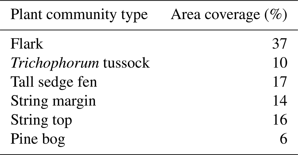
For modelling the string top CO2 fluxes for the time span from June 2017 to June 2019, to be used for pine bog (Sect. 2.4), the chamber-based fen ecosystem fluxes were scaled to match the EC-based fen fluxes. This was done similarly to Piilo et al. (2020), by first upscaling the chamber fluxes of the main PCTs of the fen to the ecosystem scale according to their relative areas within 200 m from the EC tower (Table 2). The PCT-specific fluxes were presented in more detail by Heiskanen et al. (2021).
Table 3Coefficients for scaling the chamber-based ER and GPP fluxes.
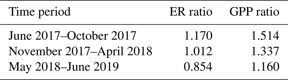
The mean ratios between the EC-based and upscaled chamber-based ER and GPP fluxes were used for scaling the chamber flux data (Table 3). For ER, the mean ratio was calculated from all data, while the mean GPP ratio was calculated from the daytime data (from 06:00 to 18:00 LST, local standard time).
2.2.3 Eddy covariance data gap-filling and partitioning
The EC flux time series of both the pine forest and fen ecosystems had substantial gaps due to equipment failures, wind sector exclusions, and quality control filtering applied during the post-processing of the data. In total, 86 % and 91 % of the forest CO2 flux data were gap-filled in the time series of 11 June 2017–10 June 2018 and 11 June 2018–10 June 2019, respectively. During the growing seasons, i.e. in 11 June–31 October 2017 and 11 June–31 October 2018, the gap-filling percentage was 77 % and 84 %, respectively. In total, 64 % and 63 % of the fen CO2 flux data were gap-filled in the time series of the first and second years, respectively. The contribution of each data filtering step is shown in Table S1 in the Supplement.
For gap-filling the pine forest CO2 fluxes during the winter, when the data coverage was lowest but the fluxes relatively small and stable, we averaged the measurement data pooled into two soil temperature categories, i.e. over and under −2 ∘C at the 10 cm depth. The mean fluxes were 0.0173 and 0.0103 in the warmer and colder category, respectively. The winter period was determined based on the timing of frost at 10 cm depth, which occurred in 31 September 2017–24 April 2018 and 30 September 2018–20 April 2019.
The growing season pine forest CO2 flux data and the entire fen CO2 flux data time series were gap-filled using a machine learning method called extreme gradient boosting (XGBoost; Chen and Guestrin, 2016). XGBoost is a decision-tree-based ensemble method in which trees are built in a sequential manner so that each tree corrects for the errors in the previous trees. XGBoost has been shown to perform well, even with long gaps in the EC data (Zhu et al., 2022; Irvin et al., 2021). The environmental variables that were used to predict NEE were photosynthetic photon flux density (PPFD), air temperature, relative humidity, vapour pressure deficit (VPD), soil temperature at −10 cm, soil temperature at −5 cm, and soil moisture at −10 cm.
First, we optimised the hyperparameters of the model using a grid search to control for overfitting and to select the best model architecture. The hyperparameters that were optimised control for the maximum depth of a tree (“max_depth”), the subsample ratio of columns when constructing each tree (“colsample_bytree”), learning rate (“learning_rate”), and the minimum number of samples required to create a new node in a tree (“min_child_weight”). The selected hyperparameters were 0.8 for colsample_bytree, 0.05 for learning_rate, 20 for max_depth, and 9 for min_child_weight. The squared error was used as the loss function. Model performance for the more sparse pine forest data was evaluated using 10-fold cross-validation, resulting in the coefficient of determination (R2) of 0.88 ± 0.02 and the mean squared error of 0.003 ± 0.0006 (Fig. S3 in the Supplement). Further details of the model performance and justification for gap-filling the EC flux time series with a high proportion of missing data are presented in Sect. S3.
The ER and GPP fluxes were partitioned based on environmental response functions that were fitted to the gap-filled NEE data. A rectangular hyperbola was used to model the dependency of GPP on PPFD (e.g. Whiting, 1994), while the exponential model of Lloyd and Taylor (1994) was used for ER. For the pine forest flux parameterisation, air temperature was used during the growing season, while soil temperature (Ts) at the 10 cm depth was used for the other periods; for the fen, Ts at the 10 cm depth was used for the whole year. For fitting the parameters of the ER function, nighttime data were used (PPFD < 30 ). The activation energy parameter (E0) of the respiration function was fitted first with a 91 d moving window, after which the base respiration rate at 10 ∘C (R10) was fitted to the data within a moving window of 7 d. The fitting of the GPP function was performed in a moving window of 3 d, using the daytime flux data (PPFD > 30 ). For gap-filling the CH4 fluxes measured at the fen, a simple moving average interpolation of the half-hour fluxes was used. A moving average window of ± 1, 2, 4, 8, 16, or 32 d was used, depending on the length of the gaps in data. In total, 69 % and 70 % of the CH4 flux data were gap-filled in the time series of the first and second years, respectively (Table S1 in the Supplement).
2.2.4 Lake CO2 and CH4 flux measurements
The diffusive fluxes of CO2 and CH4 were measured on the intermediate-sized (1.5 ha) Lake Jänkälampi, with mineral sediment (MS), and on the larger Lake Jänkäjärvi, with organic sediment (OS; Fig. 1). On Jänkäjärvi, CH4 ebullition was also measured. The lakes are hereafter referred to as the MS and OS lakes, respectively. The MS lake fluxes were measured on 5 d during June–October in 2017 and another 5 d during June–September 2018. The OS lake fluxes were measured bi-weekly during June–August 2017.
The flux measurements were conducted with floating flux chambers, while the CH4 ebullition was determined from both chamber and floating bubble collector data. The diffusive fluxes of the MS lake were measured with an opaque aluminium chamber (60 cm × 60 cm × 30 cm) at 20 m from the north shore. The chamber air was mixed with a battery-driven fan. The closure time was 7 min, after which the chamber was ventilated for 3 min. The changes in CO2, CH4, and H2O mixing ratios inside the chamber were measured using a closed-path laser-based gas analyser (Picarro G2401; Picarro, Inc., USA) connected to the chamber via a 50 m long inlet tube (Teflon; inside diameter 3.1 mm). On the OS lake, floating chambers with a volume of 8 L and an area of 0.05 m2 were applied, using a 30–60 min closure. Four samples (30 mL) of the gas space were drawn using polyethylene syringes, and the samples were stored in 12 mL glass vials flushed with sample air. Samples were analysed within a month, using a gas chromatograph equipped with electron capture, thermal conductivity, and flame ionisation detectors (Agilent 7890B, with a Gilson GX-271 autosampler). We tested CO2 fluxes against those determined using an online CO2 sensor (K33 ELG CO2 module; Senseair) in three of the chambers and obtained similar flux values. In all, 5 to 10 chambers were deployed at a time. The chambers were lined with a rope, anchored at both ends, so that they captured the open-water section of the lake from near-shore towards the lake centre. The chambers captured some ebullition events, and these were included as bubble flux. In addition, funnel bubble collectors with an area of 0.03 m2 were floated. Auxiliary flux measurements from three lakes outside the study area were conducted with the same method as for the OS lake. These measurements were utilised to assess the representativeness of the flux data collected on the MS and OS lakes.
The diffusive fluxes of CO2 and CH4 were calculated from the change in the CO2 and CH4 mixing ratios inside the closed chamber. The rate of change was calculated with linear regression based on ordinary least squares, similar to the fen ecosystem chamber measurements by Heiskanen et al. (2021).
The measurement data of diffusive fluxes were screened to reject cases with a non-linear concentration change and disturbances due to chamber leakage and ebullition events. The number of accepted/total data of the MS lake fluxes was in 2017 and in 2018. The number of accepted/total OS lake data was for diffusive CO2 fluxes and for diffusive CH4 fluxes. There were ebullition events in 7 % of the individual flux measurements, and this ebullition frequency was used to estimate the total ebullition-induced flux over the ice-free period.
2.3 Abiotic and biotic environmental measurements
In addition to the C flux measurements, meteorological and environmental variables were measured continuously at and close to the flux measurement locations in the pine forest, fen, and lake ecosystems. Air temperature, precipitation sum, and snow depth were measured at the weather station of the Finnish Meteorological Institute, located between the pine forest and fen EC measurement sites. Air temperature and humidity (Vaisala; HMP230), global and reflected radiation (Kipp & Zonen; CM7), and downward and upward PPFD (Kipp & Zonen; PQS1) were measured at the forest and fen sites at heights of 14 and 3 m, respectively. The water vapour pressure deficit was calculated from air temperature and relative humidity according to Jones (2013). Forest soil temperature was measured at 5 and 10 cm depths (Onset; HOBO) and soil moisture at 10 cm depth (Onset; HOBO). Ts profiles at the fen were measured from a string (at 10, 30, 50, 75, and 105 cm depth) and flark (at 10, 30, and 50 cm depth; IKES Pt100 sensors). The water table level (WTL) was measured manually from the flux chamber positions at the fen and OS lake, while the WTL of the MS lake was measured with a pressure sensor (Onset; HOBO U20) at the floating flux chamber position. Lake water temperature (Onset; HOBO Pendant) was measured at the same position at 10 cm from the lake bottom.
The ice-free period of the flux measurement lakes was determined from air temperature data and repeat digital photographs at the fen site (Linkosalmi et al., 2022). In October 2018, the lake freezing was recorded with a temperature and pressure logger (Onset; HOBO). The freezing occurred after the air temperature remained continuously below 0 ∘C for 3 d, with no subsequent exceedances. The timing of thaw was determined from the snowmelt and ice thaw at the fen.
We defined meteorological drought based on the atmospheric VPD as the period during which the daily maximum VPD (VPDmax) exceeded 20 hPa (Lindroth et al., 2007; Aurela et al., 2007).
The Standardised Precipitation Evapotranspiration Index (SPEI), which takes into account both precipitation and potential evapotranspiration in determining drought conditions (Vicente-Serrano et al., 2010), was used as a climatological reference for the study period. Monthly SPEI data covering the years 1950–2018 for the 0.5∘ × 0.5∘ grid cell including Kaamanen were extracted from the global SPEI database (SPEIbase v2.6; https://spei.csic.es/database.html, last access: 19 October 2021).
2.4 Estimation of pine bog fluxes
In the subarctic aapa mires, pine bogs typically form narrow zones bordering forests and peatlands. Conducting direct EC flux measurements on them is challenging, as the fetch is too limited for the EC method. Thus, the fluxes of the two pine bog ecosystems within the study area were not directly measured but, to enable regional upscaling, were modelled based on the fluxes measured in the forest and fen ecosystems. The use of forest and fen fluxes was considered appropriate because, first, the tree species composition in pine forest and pine bog is similar, and, second, the peat soil ground layer vegetation of pine bog is similar to that of the string top PCT at the fen (Table A1).
For estimating the pine bog fluxes, the total forest flux was assumed to consist of the flux of trees and the flux of the other forest ecosystem elements,
and, similarly, for the pine bog ecosystem,
The “trees” fluxes were assumed to be proportional to tree biomass, i.e.
where a is the tree biomass ratio between pine bog and pine forest (a = 0.52 and 0.16 for treed and sparsely treed pine bogs, respectively; Table A5; Sect. S4). Assuming further that the ground layer (“other”) fluxes in both the forest and pine bog equal the flux of the fen's driest PCT, i.e. string top,
Equations (2)–(5) show that the GPP and ER fluxes for the pine bog can be estimated as follows:
where Fforest and Fstring top are obtained from measurements.
2.5 Upscaling fluxes to landscape level
The CO2 and CH4 fluxes of different ecosystems were upscaled to the landscape-level by taking into account the areal contributions inside the 7 km2 study area (Tables 1 and A7) and summing the half-hourly area-weighted NEE, GPP, ER, and CH4 flux estimates of each ecosystem. The pine forest and pine bog daily average growing season CH4 flux estimates were taken from the literature (Bubier et al., 2005; Dinsmore et al., 2017), which were further calculated for 180 d long growing seasons at Kaamanen.
The annual CO2 and CH4 balances for lakes were derived from the results of Kou et al. (2022), who modelled these fluxes for the Kaamanen catchment with the Arctic Lake Biochemistry Model (ALBM). The ALBM is a one-dimensional process-based model operating on a daily time step (Tan et al., 2015, 2017). For Kaamanen, it was calibrated with the flux measurements described in Sect. 2.2.4 and driven with local meteorological data (Kou et al., 2022).
2.6 Estimating flux uncertainty
The uncertainty in the EC-based CO2 and CH4 fluxes of the pine forest and fen ecosystems were estimated by taking into account the most significant error sources. First, the uncertainty related to low-turbulence screening was estimated by filtering the data with 100 bootstrapped u∗ thresholds and gap-filling each of the resulting time series. The related uncertainty was defined as the standard deviation of the 100 gap-filled 30 min NEE values. Second, to estimate the random measurement uncertainty, we binned the measured data into 0.2 (pine forest) or 0.1 (fen) wide bins and calculated the standard deviation of model residuals for each bin. The linear relationship between this standard deviation and the magnitude of the flux was estimated separately for negative and positive fluxes and used to estimate the uncertainty in the measured data (Richardson et al., 2008). Third, the uncertainty due to gap-filling with XGBoost was estimated following the procedures detailed by Irvin et al. (2021). This uncertainty component was estimated from an ensemble of 10 models that were fitted using bootstrapped data, and the uncertainty intervals were calibrated using Platt scaling as an additional post-processing step.
To estimate the uncertainty in the annual balances, the uncertainty related to u∗ was determined as the standard deviation of the 100 bootstrapped balances. Also, the gap-filling uncertainties were determined using a bootstrapping approach. For winter, we resampled the wintertime data 100 times with replacement and calculated alternative balances. For the growing season, we used the ensemble of 10 XGBoost models to calculate alternative balances. In both cases, the gap-filling uncertainty was determined as the standard deviation of the balances.
For the flux-chamber-based monthly CO2 and CH4 flux sums of the lake ecosystem, the measurement uncertainty was estimated as the standard deviation of the flux data from the repeated chamber closures. The uncertainty in the annual CO2, CH4, and C flux sums were accumulated as the root sum square of individual uncertainties.
For the modelled pine bog fluxes, both for treed and sparsely treed bogs, the uncertainty was combined from the pine forest string top flux uncertainties proportionally to their contribution to the derived flux. The string top flux uncertainty was estimated by combining the uncertainty due to the estimated parameters of environmental response functions and the flux variation among the chamber plots (Heiskanen et al., 2021).
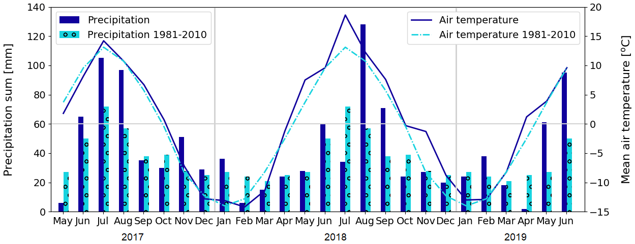
Figure 3Monthly precipitation sum and mean air temperature at Kaamanen, and the corresponding 30-year averages (Pirinen et al., 2012) measured at the Ivalo weather station (68∘36′ N, 27∘25′ E; 59 km south of Kaamanen).
The landscape-level flux uncertainty was calculated by combining the total uncertainties in each ecosystem, excluding lakes due to differing data sets, proportionally to their areal coverages (Table 1). All uncertainty estimates reported for C balances refer to the 95 % confidence intervals.
2.7 Statistical analysis
The estimates of ER, GPP, NEE, and CH4 fluxes of pine forest and fen ecosystems were compared between the two growing seasons using the Z test, for which we produced full flux time series with uncertainty estimates. Welch's t test was used for comparing the monthly average lake fluxes between the 2 years, as the compared data comprised of a sample of measured fluxes.
For identifying the main environmental drivers of the pine forest CO2 flux, a linear regression model was estimated to explain the 5 d averaged GPP and ER fluxes derived from the measured EC data. The FR data were normalised to 10 ∘C (denoted as FR10), while the FGPP data were normalised to a near-optimal PPFD level of 1200 (denoted as FGPP1200; Laurila et al., 2001).
The following fixed explanatory 5 d variables were tested in the models: precipitation sum, average VPDmax, soil moisture and temperature at a depth of 10 cm, air temperature, and daily maximum PPFD. Ts was included in the final analysis, while air temperature was excluded because these variables were strongly correlated (Pearson's R = 0.96 in the FR data and R = 0.93 in the FGPP1200 data), and Ts showed higher absolute correlation with the response variables. The MODIS normalised difference vegetation index was also tested as an explanatory variable, but it was excluded from the final analysis, as it strongly correlated with Ts (Pearson's R = 0.87 in the FR data and R = 0.89 in the FGPP1200 data). For the final models, the explanatory variables were chosen with a stepwise procedure to both directions by minimising Akaike's information criterion value. To evaluate the relative impact of each explanatory variable, the standardised regression coefficients were calculated. Data analyses were conducted in R (R Core Team, 2021) with the MASS (Venables and Ripley, 2002) and MuMIN (Barton, 2020) packages.


Figure 5Daily average (a) forest soil temperature measured at 10 cm depth and snow depth, (b) fen peat temperature measured from strings and flarks at 10 cm depth, and (c) MS lake water temperature at the floating chamber position 10 cm from the bottom.
3.1 Environmental conditions
We studied CO2 and CH4 fluxes across different ecosystem types in Kaamanen from June 2017 to June 2019. The growing seasons (May–October) of 2017 and 2018 differed from each other in terms of their meteorological conditions, which affected the CO2 and CH4 exchange between the atmosphere and ecosystems. The early growing season in 2017 was colder than the corresponding period in 1981–2010 on average (Pirinen et al., 2012), with May being 1.9 ∘C and June 1.4 ∘C colder (Fig. 3). The summer months of June–August were rainy in 2017, which was reflected in cloudiness that decreased the incoming solar radiation, with July in particular being cloudy (Fig. 4). In contrast, the spring of 2018 was warm, with May being 3.8 ∘C warmer than the 30-year May average. In July 2018, a widespread drought and heatwave event in northwestern Europe reached Kaamanen and caused the monthly mean air temperature to rise to 18.6 ∘C, which was 5.3 ∘C higher than the 30-year July average. Additionally, the monthly precipitation sum was less than half of the 30-year average (34 and 72 mm, respectively). After the drought, the following August and September were also warmer than the corresponding 30-year averages, by 1.5 and 1.9 ∘C, respectively, but the precipitation sum was then double the 30-year average. Spring 2019 was characterised by a dry and warm April (3.7 ∘C above the long-term average) and rainy weather in May and June. Lake water levels were visibly lower in 2018, exposing the shoreline sediments of shallow lakes, for instance, in the MS lake of this study.
The forest soil freeze and thaw occurred each year at the end of October and in mid-May, respectively (Fig. 5a). In late autumn 2018, the forest Ts decreased from 8 to 1 ∘C in just 20 d between 23 September and 13 October, which was due to the lack of snow cover. In the fen, the surface peat of the strings froze concurrently with the forest soil (Fig. 5b). However, the thaw occurred slightly earlier in the strings than in the forest, where trees shaded the surface. The continuous water saturation in the flark peat led to weaker peat temperature responses to changing air temperature than in the dryer strings. The lake water temperature, measured only during the ice-free periods of 2017 and 2018 (Fig. 5c), was affected, in addition to air temperature, by the incoming flow to the lake and by the water level. Following the air temperatures, the forest soil, fen peat, and lake water temperatures were higher in July 2018 than in 2017.
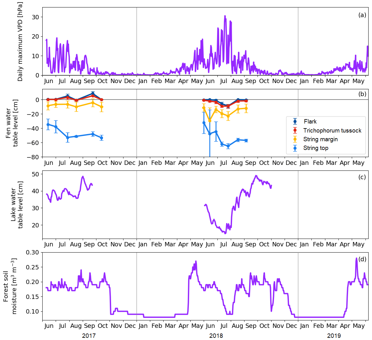
Figure 6(a) Daily maximum vapour pressure deficit. (b) Mean water table level at the main plant communities of the fen. Error bars represent the standard deviation. (c) Water table level at the floating chamber position in Lake Jänkälampi. (d) Forest soil moisture at 10 cm depth.
Table 4Estimated ice-free period start and end dates for the studied lakes.
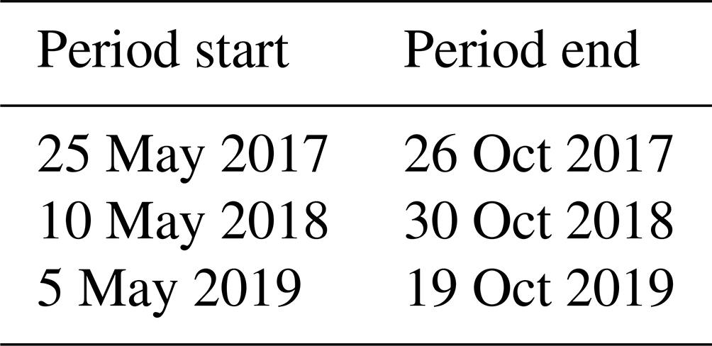
The ice-free period of the measured lakes lasted for 167 and 176 d (from May to October) during the first and second study years, respectively (Table 4).
The meteorological drought lasted from 2 July to 1 August 2018 (Fig. 6a). The drought limit of daily VPDmax = 20 hPa was exceeded on 13 d in total in 2018, while no exceedances took place in 2017. The average daily maximum VPD in 2 July–1 August 2018 was 16.9 hPa, while, during the same period in 2017, it was 9.4 hPa. The corresponding daily air temperatures were 18.5 and 14.2 ∘C, respectively. The highest daily maximum VPD of 31 hPa was observed on 18 July 2018. VPD responded rapidly to the reduced amount of water in the environment, while the water table level in the fen, the water depth of lakes, and the forest soil moisture decreased gradually as the drought developed (Fig. 6).
Within the fen, the WTL varied strongly among the plant community types (Fig. 6b). In the flark and Trichophorum tussock PCTs, WTL was close to or at the peat surface most of the time, while in elevated strings it was deeper, away from the peat surface, fluctuating between −10 and −20 cm in string margins and between −30 and −70 cm in string tops. The drought decreased the WTL in all plant communities simultaneously, and by mid-August, the WTL had recovered to a normal level, except for the string tops.

Figure 7The 1-month (July) and 5-month (May–September) Standardised Precipitation Evapotranspiration Index (SPEI) at Kaamanen in 1950–2018. Positive SPEI values denote moist conditions and negative values drought conditions. The years 2017 and 2018 are marked with shading.
The water depth of the MS lake was within 30–40 cm (Fig. 6c), and it dropped in June–July 2018 to less than 20 cm at the centre of the lake. This drawdown was associated with a shoreline retreat of 6 to 8 m. However, after the first rainfall in 3–5 August, the water depth quickly reverted to the pre-drought level. Our field observations and visual interpretation of satellite and drone imagery suggest that the water level drop magnitude was uniform in the waterbodies within the study area.
The annual cycle of the soil moisture measured in the pine forest showed a low moisture content (< 0.1 m3 m−3) during winter and fluctuations after the soil thaw (Fig. 6d). During both springs, the water availability in soil was at its maximum in 10–14 May due to melting snow. The drought during summer 2018 was clearly indicated by the soil moisture data that showed a drastic drop from 0.2 to 0.1 m3 m−3 between 23 June and 22 July. After the rainfall in the beginning of August, the soil moisture rose in a few weeks to the average growing season level. Thus, even though the meteorological drought was already over at the beginning of August, the water availability to vegetation was not yet fully recovered.
In terms of the drought index (SPEI), the drought event in July 2018 was the eighth most severe drought in Kaamanen between January 1950 and December 2018 (Fig. 7). However, the drought event was relatively short, and the 5-month SPEI between May and September was close to neutral.

Figure 8Pine forest gap-filled fluxes. Weekly averaged (a) and cumulative (b) CO2 flux. Weekly averaged ecosystem respiration (c) and gross primary productivity (d).
3.2 Ecosystem CO2 and CH4 fluxes
3.2.1 Pine forest fluxes
The pine forest acted as a net CO2 sink during both study years. The annual CO2 balances (with the 95 % confidence intervals) during the first and second study years were −126 ± 21 and −101 ± 19 g C m−2, respectively (Fig. 8b; Table A6). For other evergreen needleleaf forests in northern Fennoscandia, the observed balances have been smaller in magnitude; the Scots pine forest at Värriö in northern Finland was a CO2 sink in 2012–2014 (−48 to −7 g C m−2) and a small source in 2015 (14 g C m−2; Kulmala et al., 2019), while the Norway spruce forest at Kenttärova in northern Finland had a close-to-neutral balance (on average −2 g C m−2; Aurela et al., 2015).
There were two periods when the CO2 fluxes behaved differently between the 2 study years, due to differing meteorological conditions. First, even though the summer was warmer in 2018 than in 2017, and thus one could expect enhanced respiration, the ER fluxes of the pine forest ecosystem were on average similar during the growing seasons. This was due to the rainy period in June–August 2017 (Fig. 3), as a result of which the forest soil remained saturated or nearly saturated in water during the whole growing season (Fig. 6d). As the forest soil moisture content was continuously close to the maximum water-holding capacity, the effect of abundant precipitation emerged as increasing lake water table levels (Fig. 6c). We suspect that the stronger ER temperature response observed in June–August 2017 was caused by enhanced heterotrophic soil respiration (Fig. A1 in the Appendix), which is known to increase with soil moisture until near-saturation with water (Orchard and Cook, 1983; Moyano et al., 2012; McElligott et al., 2017; Du et al., 2020).
The second period of dissimilar behaviour in CO2 fluxes was observed when the drought and heatwave discussed above limited GPP fluxes; compared to the previous year, the GPP sum in 22 July–17 August was 35 g C m−2 lower in 2018 (Z test; p = 0.003; Fig. 8d). The daily maximum VPD surpassed the 20 hPa limit, indicating meteorological drought, for the first time on 2 July and the last time on 1 August 2018 (Fig. 6a), during which period the average air temperature was 5 ∘C higher than in the previous year (Fig. 3). In July 2018, the forest soil moisture at 10 cm depth also dropped by 50 % from the normal growing season level, decreasing to 0.1 m3 m−3 on 22 July (Fig. 6d). Soil moisture recovered to a normal level 3 weeks later on 13 August.
There is an evident discrepancy between the timing of the meteorological drought and the reduced ecosystem CO2 fluxes. The response to drought in plants occurs both in roots, where water availability through soil is a key factor, and in the stomatal openings in leaves, where the gas exchange is affected by stomatal control due to VPD. The tighter stomatal control is due to the high VPD limits C assimilation (Martín-Gómez et al., 2017), and in Scots pine trees, this has been estimated to occur at a VPD of 8 hPa, while at approximately 28 hPa the stomata are fully closed (Büker et al., 2012). The drought seemed to have an effect on the CO2 exchange until 18 August, even though soil moisture and VPD hardly had any direct effect anymore, as only after this date were the magnitude of ER and GPP fluxes not continuously lower compared to the previous year. This lagged effect could be caused by embolism, defoliation, or root degradation (Aguadé et al., 2015) or by weakened mycorrhizal symbiosis in the roots (Muilu-Mäkelä et al., 2015). Gao et al. (2017) also found that the GPP of a southern boreal Scots pine forest was suppressed during a severe soil moisture drought in the summer of 2006, as the plants regulated their stomata due to high VPD.
Table 5Standardised regression coefficients (± standard error) for the explanatory variables of the linear regression model for EC-based FGPP1200 and FR10. The adjusted coefficient of determination (), normalised root mean square error (nRMSE; RMSE divided by the range of response variable values), and degrees of freedom (df) are also shown.
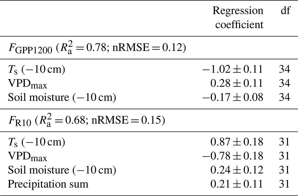
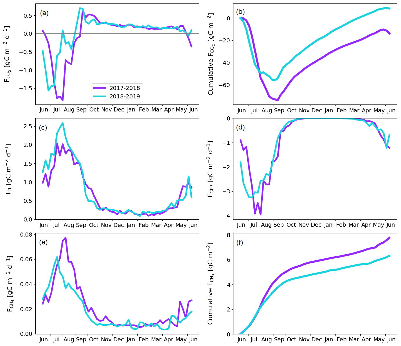
Figure 9Fen gap-filled fluxes. Weekly averaged CO2 (a), ER (c), GPP (d), and CH4 (e) flux. Cumulative CO2 (b) and CH4 (f) flux.
According to the linear regression model, the main environmental factors affecting the radiation-normalised GPP flux (FGPP1200) of the pine forest were Ts, VPDmax and soil moisture (Table 5). The magnitude of FGPP1200 increased with increasing Ts and soil moisture and decreased with increasing VPDmax. The positive correlation with soil moisture originated from the anomalously low moisture levels during the 2018 drought (Fig. 6d). The temperature-normalised respiration (FR10) was affected by Ts, VPDmax, soil moisture, and precipitation sum (Table 5). FR10 increased with increasing Ts, soil moisture, and precipitation sum and decreased with increasing VPDmax.
3.2.2 Fen fluxes
The fen ecosystem was a small net CO2 sink of −14 ± 17 g C m−2 and a small net CO2 source of 9 ± 11 g C m−2 during the first and second years, respectively (Fig. 9b; Table A6). There were three periods during which either CO2 or CH4 fluxes diverged between the years, namely the start of the growing season, the warmer-than-average growing season of 2018, and the drought and heatwave event in 2018.
The warm growing season increased the ER flux sum by 32 g C m−2 (Z test; p = 0.124) during 11 June–23 September 2018 (mean air temperature 13.2 ∘C) compared to 2017 (10.5 ∘C). Half of this difference, 16 g C m−2 (Z test; p = 0.043), accumulated in just 26 d, 17 July–12 August, when the temperature difference between the years was largest (13.4 and 17.9 ∘C in 2017 and 2018, respectively).
The earlier start for the growing season in 2018 resulted in a higher CO2 uptake in 11–30 June compared to the previous year (Fig. 9; Table A6); the balances of this period were −5 ± 13 and −20 ± 17 g C m−2 in 2017 and 2018, respectively. This was due to the nearly doubled GPP (Z test; p < 0.001), which was 27 ± 3 and 49 ± 4 g C m−2 in 2017 and 2018, respectively. The increase in the net CO2 uptake in northern mires due to earlier snowmelt and warm spring temperatures has been reported previously by, for example, Aurela et al. (2004) and Sagerfors et al. (2008). The differences in CO2 exchange between the microforms of the fen were studied in more detail by Heiskanen et al. (2021), who found that the magnitude of ER and GPP increased gradually from the wettest PCT, i.e. flark, to the driest one, i.e. string top. However, the variation in the net CO2 uptake among the microforms was weaker than in the two flux components. The increased GPP due to warm spring weather was observed in all main microforms. However, the simultaneous increase in ER led to a significantly (p < 0.05) higher net CO2 uptake only in string tops, when comparing the early growing seasons of 2017 and 2018 (Fig. A2).
The higher CO2 uptake during the early growing season of 2018 was offset by the decreased uptake due to the drought and heatwave event in 8 July–4 August 2018. The GPP sum was 17 g C m−2 smaller (Z test; p = 0.229) during this period in 2018 than in 2017 (Fig. 9d). As discussed above, the drought was observed as higher-than-average temperatures (Fig. 3), an elevated VPD (Fig. 6a), and water level drawdown by 5–20 cm at the fen microforms (Fig. 6b). These anomalies likely caused drought stress in the mire plants (Alm et al., 1999). The drought stress reduced GPP, and the high temperatures increased ER compared to the previous weeks and the same time period during the previous year (Fig. 9c and d). The CO2 uptake decreased during this period, and at the end of the period the fen ecosystem even turned into a CO2 source. Unlike the increased CO2 uptake during the early growing season, which could be allocated largely to the string plant communities, the drought affected plant communities in all microforms (Heiskanen et al., 2021). The CO2 exchange in flarks, including Trichophorum tussocks, was immediately affected by the lowering WTL in July and August 2018 (Fig. 6b), while the drier string communities were affected to a lesser extent.
While the fen was an annual net CO2 sink, it also acted as a CH4 source to the atmosphere during both study years. The annual CH4 balance was 7.8 ± 0.2 and 6.3 ± 0.3 g C m−2 during the first and second study years, respectively (Fig. 9f). The flark, Trichophorum tussock, and string margin PCTs contributed 98 % of the emissions, with string margins accounting for 44 % of the emissions during the growing season of 2017 and all three having similar emissions in 2018 (Heiskanen et al., 2021).
The drought decreased the annual CH4 emissions, mostly during 21 July–28 August 2018, when the emissions were 0.8 g C m−2 lower (Z test; p < 0.001) than during the same period in the previous year (Fig. 9e). Notably, the decrease in CH4 emissions occurred a few weeks after the meteorological drought begun and continued well after the WTL had reverted to the pre-drought level. The decrease in CH4 emissions is likely due to both the reduced release of carbon compounds by plant roots and increased oxic soil zone, which reduced CH4 production and increased CH4 oxidation (Strack and Waddington, 2007; White et al., 2008; Deppe et al., 2010). The lagged recovery of CH4 flux coinciding with the GPP recovery indicates the link between methanogenesis and plant root exudates. Unfortunately, the uncertainties in the monthly CH4 balances derived from the manual chamber measurements were large, and the lower emissions could not be allocated to any specific PCT. However, the CH4 emissions from flarks were larger in 2018 than 2017, which suggests that the drought-induced decrease in emissions occurred for the Trichophorum tussock and string margin PCTs that had a lower WTL (Fig. 6b; Heiskanen et al., 2021). The drought, which covered large parts of northwestern Europe, did not affect the CO2 and CH4 exchange at Kaamanen as much as it did at more southern mires, where the drought duration was longer, although the water level drawdown was similar in magnitude (Rinne et al., 2020).
The total carbon balance, i.e. the sum of the CO2 and CH4 fluxes, showed that the fen was an annual carbon sink, −7 ± 17 g C m−2, and a carbon source to the atmosphere, 15 ± 11 g C m−2, in the first and second study years, respectively (Table A6). The lower net CO2 uptake during the drought period contributed most of the difference between the years. Previous studies at the Kaamanen fen show that the ecosystem has been on average a larger annual CO2 sink, −22 g C m−2 (from −4 to −53 g C m−2) during 1997–2002 (Aurela et al., 2004), and a similar average annual CH4 source of 6 g C m−2 in 1995, 1997–1998, and 2011–2016 (Hargreaves et al., 2001; Piilo et al., 2020).
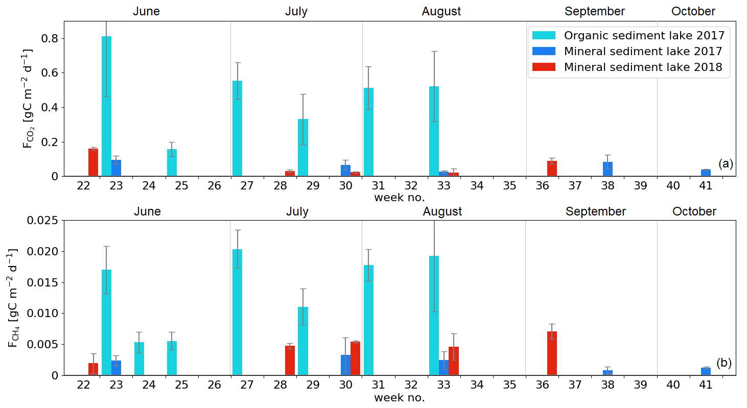
Figure 10Weekly average lake CO2 (a) and CH4 (b) diffusive fluxes. Error bars represent the standard deviation of individual chamber measurements in each week.
3.2.3 Lake fluxes
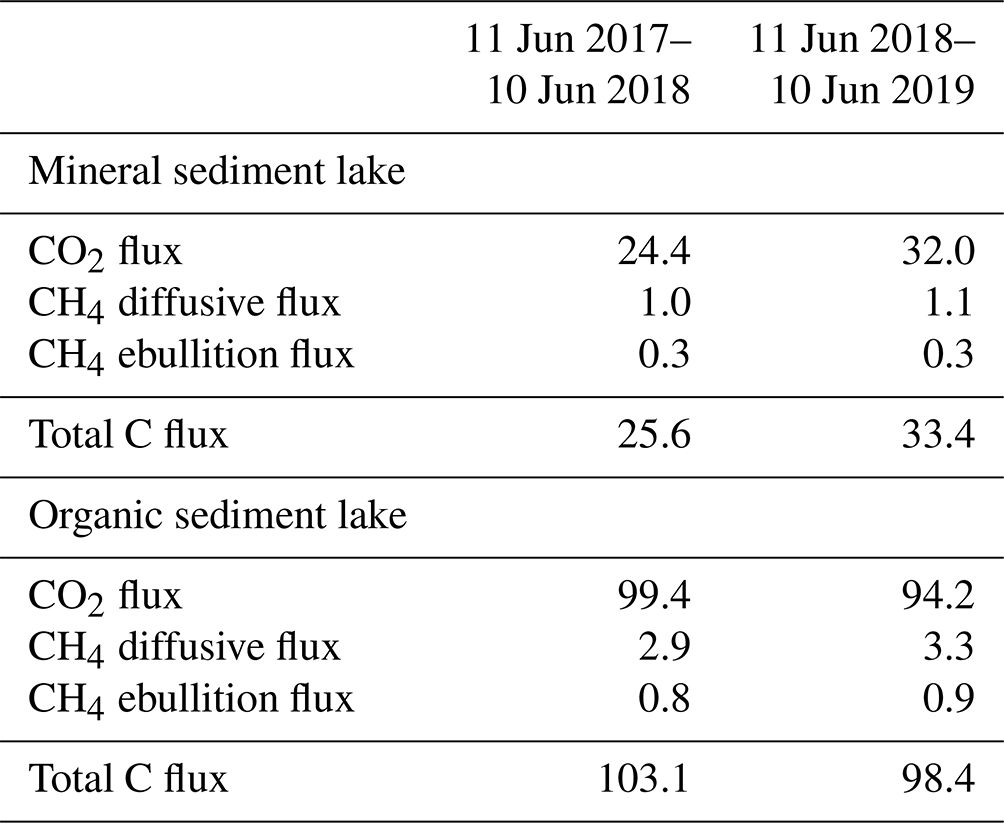
The measured CO2 fluxes of the OS and MS lake were on average 0.45 and 0.06 during the ice-free period, and the mean CH4 fluxes were 0.014 and 0.003 , respectively (Fig. 10). The large difference in the flux rates between the lakes was most likely caused by the fact that the OS lake is situated immediately downstream of the fen (Fig. 1). Due to the location, the OS lake receives transported organic carbon (OC) in the streamflow and has a higher lake water total organic C content than the MS lake (9 vs. 5 mg L−1) and a higher C content in its sediment (30.3 % C of dry mass) than in the MS lake sediment (5.5–22.6 % C, depending on location; Table A8). Based on the ALBM model calculations (Kou et al., 2022), calibrated with the flux observations at the MS and OS lakes (Sect. 2.5), the annual CO2 emissions were on average 28 g C m−2 from the MS lake and 97 g C m−2 from the OS lake. The modelled CH4 emissions were 1.4 g C m−2 from the MS lake and 4.0 g C m−2 from the OS lake (Table 6).
Table 6Modelled annual CO2 and CH4 balances (g C m−2) of the MS and OS lakes during the 2 study years (Kou et al., 2022).
The CO2 emissions of the OS lake (0.2–0.8 ; Fig. 10a) were similar in magnitude, for instance, to those (0.3–1.4 ) observed for Lake Stortjärn in Sweden, which is a northern boreal lake located adjacent to a mire (Denfeld et al., 2020). In lakes with less organic carbon in the water, the net CO2 emissions are lower, yet we did not observe CO2 uptake by either of the studied lakes. In a similar shallow subarctic lake next to a fen at Abisko in Sweden, Jammet et al. (2017) found high CO2 emissions of 33.3 g C m−2 during the spring period of 41 d, but the photosynthetic CO2 uptake during summer reduced the net emission of the ice-free period to 8.9 g C m−2. Lohila et al. (2015) estimated an annual CO2 balance of 33 g C m−2 for the shallow parts of the large subarctic Lake Pallasjärvi in Finland and recorded a small CO2 uptake during midday in the summer months. Also, small annual CO2 emissions, 11.5 g C m−2, were estimated for the small (9.6 ha) Lake Kipojärvi located near Kaamanen, surrounded by both an esker and a peatland (Juutinen et al., 2013). This shows that the CO2 balance of lakes varies substantially from lake to lake in the subarctic region.
The annual CH4 emissions of Lake Kipojärvi, 3.4 g C m−2, were similar to the modelled OS lake emissions. The average daily diffusive CH4 fluxes varied from 0.001 to 0.020 in this study and were similar to those reported in previous studies of boreal lakes. Denfeld et al. (2020) observed a range of 0.001–0.008 for Lake Stortjärn during the ice-free period, while Rasilo et al. (2015) found spatially highly variable CH4 diffusive fluxes of 0.008 ± 0.020 across 224 boreal lakes in Canada during summer. The length of the ice-free period can affect the annual emission of different boreal lakes considerably, as the ice cover prevents gas exchange with the atmosphere (Guo et al., 2020).
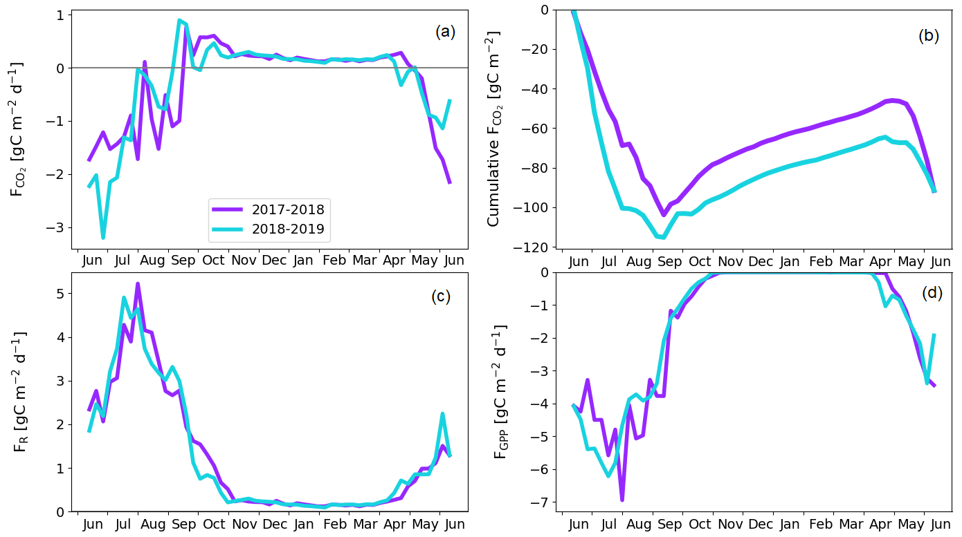
Figure 11Treed pine bog gap-filled fluxes. Weekly averaged CO2 flux (a) and cumulative CO2 flux (b). Weekly averaged ER (c) and GPP (d) flux.
Our estimate of ebullition was 22 % of the total CH4 emission. This is smaller than observed in other studies of boreal lakes, especially considering that our study lakes are mostly shallow (< 2 m deep) and thus likely to show more frequent CH4 ebullition than deep lakes (Bastviken et al., 2004). Contributions of 40 %–80 % of the total CH4 emissions have been estimated for subarctic lakes (Bastviken et al., 2004; Wik et al., 2013; Jansen et al., 2020), and the annual CH4 emissions of 1.0–8.3 g C m−2 have been observed (Bastviken et al., 2004; Thornton et al., 2015; Jammet et al., 2017). In general, there is high temporal and spatial variation in ebullition, as there are both seep and non-seep areas where CH4 bubbles emerge at the lake bottom, which complicates the ebullition estimation (Walter et al., 2006). Wik et al. (2018) found that the spatial ebullition potential was affected by the coarse detritus, buried aquatic vegetation, and redeposited peat rather than the amount of total organic carbon or CH4 in the sediment.
Both lakes showed the largest CO2 emissions in early June (Fig. 10a). However, a similar development of fluxes was not observed with CH4 (Fig. 10b). The dissimilarity between the gases is likely due to the differing production and accumulation processes. CO2 emissions are driven by the amount of incoming dissolved and particulate carbon and the rate of decomposition of that organic carbon (Kortelainen et al., 2006), while CH4 production is controlled by the substrates available for the methanogens to reduce it to CH4 in anoxic conditions in sediments (Chapin et al., 2011). CH4 concentration has been observed to be roughly constant with depth during the early summer, while CO2 is strongly stratified, with a larger concentration towards the bottom of the lake (Denfeld et al., 2020). The breakdown of thermal stratification and turnover mixing occurs around the start and end of the ice-free period (e.g. López Bellido et al., 2009). At the MS lake, the flux measurements also covered the autumn turnover mixing in September, when CO2 emissions increased compared to the previous month. The daily average CO2 flux on the MS lake was lower in July 2018 than in 2017 (Welch's t test; p = 0.01; Fig. 10), but no significant changes were observed in the measured CH4 fluxes between the years.
Both lake types emitted 96 % of the total C efflux as CO2 (Table 6). For comparison, in an extensive study of Alaskan subarctic lakes, the non-yedoma lakes emitted about 85 % as CO2 and 15 % as CH4 (Sepulveda-Jauregui et al., 2015), and in the above-mentioned 224-lake study, the CH4 diffusive fluxes contributed 8 ± 23 % to the total lake C emissions (Rasilo et al., 2015).
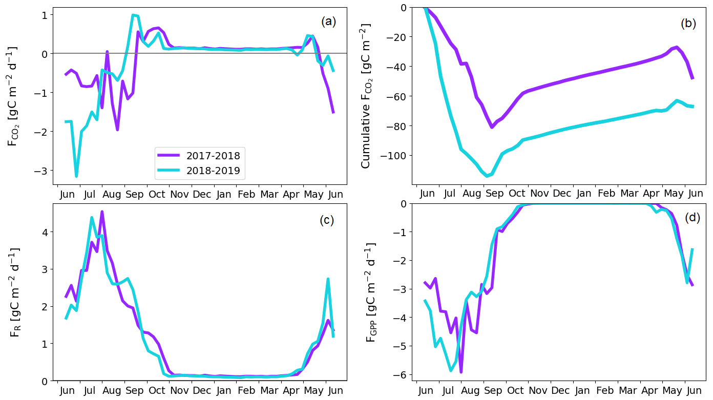
Figure 12Sparsely treed pine bog gap-filled fluxes. Weekly averaged CO2 flux (a) and cumulative CO2 flux (b). Weekly averaged ER (c) and GPP (d) flux.
3.2.4 Pine bog fluxes
The treed pine bog ecosystem between the forest and fen ecosystems covers 9.1 % of the studied landscape, and the sparsely treed pine bog covers 13.5 % and is located within the fen ecosystem in the driest parts of peatland. The annual CO2 balance of the treed pine bog ecosystem was similar in the first and second study years, −92 ± 102 and −92 ± 110 g C m−2, respectively (Fig. 11b; Table A6). The corresponding estimates for the sparsely treed pine bog ecosystem were lower and more uncertain at −48 ± 134 and −68 ± 145 g C m−2 (Fig. 12b; Table A6). The larger uncertainties in these balances compared to the forest and fen ecosystems were due to the contribution of the modelled string top fluxes, which were based on a limited number of chamber measurements (Sect. 2.4).
For both pine bog ecosystems, the GPP rates were higher during the latter year from mid-June to mid-July (Figs. 11d and 12d). This led to larger net CO2 uptake during the first part of growing season in 2018 than in 2017 (Figs. 11a, b and 12a, b). However, this difference in fluxes was more prominent in the sparsely treed pine bog. The drought event decreased the magnitude of the GPP rate similarly in both ecosystems between mid-July and mid-August 2018 compared to the previous 2 summer months and the same period in 2017 (Figs. 11d and 12d).
The pine bog ecosystem fluxes were derived from the pine forest and fen ecosystem fluxes. String tops, which were used as a proxy for a treeless pine bog, are relatively dry microsites, with a typical water table depth of 40–60 cm (Fig. 6b). As part of the bog ecosystems are wetter than the typical string tops, and as the flark PCTs at Kaamanen had lower CO2 fluxes than the string tops (Heiskanen et al., 2021), the proxy approach may bias the pine bog flux estimates. However, the use of string margin fluxes instead of the string top fluxes would not make any significant difference. The fluxes of the pine bog ground layer have been studied previously within a nearby Kipojärvi catchment by Juutinen et al. (2013), who found that in 2006 the ground layer was an annual CO2 sink of −130 ± 91 g C m−2, with an annual GPP sum of −456 ± 77 g C m−2 and ER sum of 326 ± 48 g C m−2. The ER sum was similar to that measured at the Kaamanen fen on the string top and margin PCTs (Heiskanen et al., 2021), but the magnitude of the GPP sum and thus the CO2 sink were greater for the Kipojärvi catchment (Fig. A2b). This suggests that our pine bog flux estimates might underestimate the true CO2 sink of this ecosystem.

Figure 13Landscape-level gap-filled fluxes. Weekly averaged CO2 (a), ER (c), GPP (d), and CH4 (e) flux. Cumulative CO2 (b) and CH4 (f) flux.
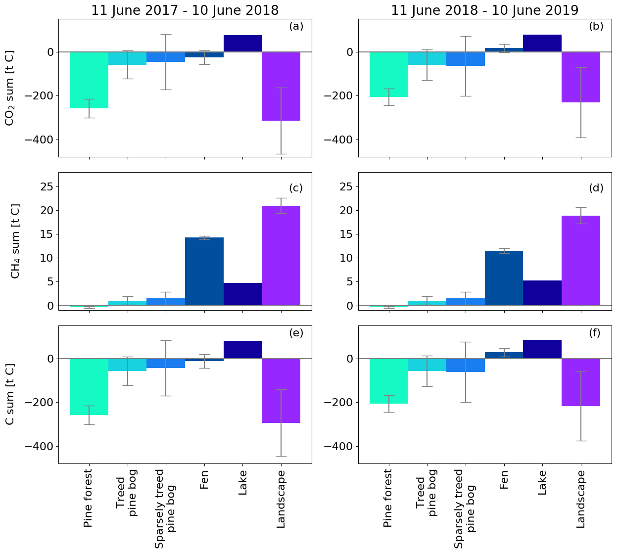
Figure 14Annual CO2, CH4, and C flux sums for different ecosystems and the landscape (Fig. 1) upscaled with the corresponding area. The CH4 flux estimate for forest is from Dinsmore et al. (2017) and for pine bog from Bubier et al. (2005). The error bars denote the 95 % confidence interval. Uncertainty estimates were not available for the modelled lake balances (Kou et al., 2022).
3.3 Upscaled landscape-level fluxes
By upscaling the ecosystem balances to our study area of 7 km2, we obtained an annual landscape-wide CO2 balance of −45 ± 22 and −33 ± 23 g C m−2 for the 2 study years. The corresponding CH4 balances were 3.0 ± 0.2 and 2.7 ± 0.2 g C m−2, and the sum of CO2 and CH4 balances were −42 ± 22 and −31 ± 23 g C m−2, respectively (Fig. 13b, f; Table A6). The pine forest ecosystem contributed to the total landscape C balance with a large CO2 sink and a minimal CH4 sink. In the evergreen forest ecosystem, the CO2 uptake period was longer than that of the fen ecosystem by 12 d at the beginning of the growing season and by 30 d at the end of the growing season (Figs. 8d and 9d), and during the first half of the growing season, the magnitude of CO2 uptake was larger in the forest (Figs. 8a and 9a). The lake ecosystem was the complete opposite, with substantial CO2 and CH4 emissions, while the fen ecosystem balances were between forest and lake, with annual net CO2 uptake and CH4 emissions, although the fen had larger CH4 emissions per unit area than the lakes. The pine bog ecosystems, which were modelled using pine forest and fen fluxes, most likely acted as CO2 sinks and CH4 sources. The ecosystem-specific CH4 emissions were much lower than the magnitude of CO2 exchange, with the exception of the fen ecosystem. The fen CH4 fluxes largely determined the landscape-level CH4 emissions (Fig. 14). The average annual terrestrial C uptake of the landscape was 338 ± 156 t C, of which 24 % was released back to the atmosphere by the lakes, resulting in a net C uptake of 256 ± 156 t C within the landscape (Fig. 14).
The studied landscape consisted of roughly an equal area of pine forest, pine bog, open peatland, and lakes (Table 1). Kou et al. (2022) studied the effect of the land-cover-type misclassification to the ecosystem and landscape C balances at Kaamanen using biogeochemical and atmospheric models. Their study area encompassed the entire 32.8 km2 catchment at Kaamanen. In a related manner, the 7 km2 area of this study partially coincided with the most southern part of the catchment. The catchment consisted of proportionally more pine forest (53 %) and less open peatland (16 %), fewer lakes (13 %), and fewer pine bogs (9 %). In contrast to this study, birch-dominated ecosystems (1 %) and mixed forests (6 %) were also present in the area. Thus, the 7 km2 study area represented almost all ecosystems found in the greater landscape area around Kaamanen. The average annual landscape CO2 balance was −104 g C m−2 and the CH4 balance 2.4 g C m−2. The larger annual landscape CO2 uptake on catchment-scale highlights the effect of the proportionally larger forested area that was effective in CO2 sequestering. Aurela et al. (2015) estimated an annual landscape-level CO2 balance of −5 g C m−2 for a 1963 km2 area in Pallas in northwestern Finland that was comprised of 71 % pine forest, 12 % open wetland, 6 % water surfaces, and 2 % treeless fell tops. Within this area, the 105 km2 Lake Pallasjärvi catchment included fewer forests and peatlands, but more lake and fell area, and the annual landscape-level CO2 balance was estimated to be 15 g C m−2. The annual CO2 uptake in Pallas was lower than in Kaamanen in spite of the much larger proportion of forests. In a study temporally overlapping our study, Chi et al. (2020) reported landscape-level C balances for a typical northern boreal forest landscape in Svartberget, Sweden, where forests covered 87 % of the area; the annual landscape-level CO2 balance was −37 g C m−2 in October 2016–September 2017 and −108 g C m−2 in October 2017–September 2018. The latter year showed a drought response similar to Kaamanen; a higher annual CO2 uptake was observed in the forest, while the mire ecosystem (9 % of the area) turned from an annual CO2 sink to a source. The annual CO2 balances of Svartberget were comparable to Kaamanen, whose pine forest had an annual CO2 balance of −78 and −119 g C m−2 during the first and second study years (Fig. 8d). In a synthesis by Virkkala et al. (2021), the mean annual NEE of 41 boreal biomes was on average −46 g C m−2 (uplands −47 g C m−2 and wetlands −38 g C m−2), i.e. the CO2 sink was lower in uplands and larger in wetlands than the mean landscape-scale sink in Kaamanen. These results not only show that there can be large spatial variation in C exchange among boreal ecosystems, e.g. forests, but also part of the variation between landscape C balances derive from the ecosystem composition.
The temporal variation in the landscape-level CO2 flux (Fig. 13) obviously depended on the flux variation in individual ecosystems, and different ecosystems showed different environmental responses. During the 2 study years, there were three periods when the ecosystem-specific fluxes clearly deviated from each other, and these differences were reflected in the landscape-level C balance. First, the warmer-than-average early growing season in 2018 increased the CO2 uptake of the fen ecosystem (Fig. 9a) and probably also the pine bog fluxes (Figs. 11a and 12a), or conversely, the colder-than-average early growing season in 2017 led to lower CO2 uptake by these ecosystems. However, equally large variation in the early growing season CO2 uptake was not observed in the pine forest fluxes, as the evergreen pine forest phenology differs from that of the largely deciduous mire. Second, the rainy peak growing season in 2017 increased the ER rates of the pine forest ecosystem compared to the same period in the next year, which was much warmer, and thus, the ER fluxes were similar (Figs. 8 and A1). Conversely, at the fen, the warm summer of 2018 increased the ER sum compared to the cool, rainy summer in 2017. This was due to the inherently different water balance between uplands and peatlands. Third, the drought period in summer 2018 decreased the CO2 uptake in both the pine forest and fen ecosystems (Figs. 8b and 9b), and the pine bogs likely showed a similar response.
The lakes in the landscape acted as CO2 sources to the atmosphere throughout the growing seasons, with peak emissions linked with the spring thaw. However, the temporal variation in the lake emissions had only a minor effect on the temporal variation in the landscape-scale CO2 fluxes, as the flux magnitude did not vary as much on the lakes as on the terrestrial ecosystems during the growing seasons (Figs. 8, 9, and 10). Integrated over the study area, the total lake emissions had a considerable effect on the landscape-scale annual balances (Fig. 14).
As the pine forest and pine bog CH4 fluxes used for upscaling were adopted from the literature (Dinsmore et al., 2017; Bubier et al., 2005), only the fen and lake ecosystem CH4 fluxes affect the annual variation in the upscaled landscape-level fluxes (Figs. 13 and 14). The CH4 emissions from the fen decreased due to the drought in 2018 (Fig. 9e), thus decreasing the annual emissions compared to the first study year (Table A6). However, as the modelled lake CH4 emissions were slightly higher during the second year (Table 6), there was only a minor difference in the annual landscape-level CH4 balance (Fig. 13f; Table A6).
During the 2 study years, the meteorological conditions were not optimal for C sequestration, as the fen on average acted as a weaker CO2 sink than in some previous years (Aurela et al., 2007) and even a source in the second year. Thus, the landscape-level CO2 uptake would probably be higher in more optimal conditions. However, the conditions favouring C sequestration differ between ecosystems, as all terrestrial ecosystems are likely to sequester more CO2 during longer growing seasons, but mires can simultaneously emit more CH4, and lakes emit more of both CO2 and CH4.
For estimating the relative radiative impact of the CO2 and CH4 exchanges in Kaamanen, the CH4 flux was translated to CO2-equivalent flux by multiplying it by the sustained global warming potential (SGWP) coefficient (Neubauer and Megonigal, 2015; Neubauer, 2021). If the CO2 and CH4 flux observed during the 2 study years continued for the next 500 years (SGWP = 14 ), then the net CO2-equivalent flux of the fen would be positive. However, in longer timescales, the fen will eventually have a negative radiative balance, even with a low annual CO2 uptake. In addition to the time-dependent contribution of fens, the annual net CO2-equivalent flux of the landscape was affected by uptake of both CO2 and CH4 by forests, i.e. a systematically negative CO2-equivalent flux, and emissions of both CO2 and CH4 from lakes, i.e. a systematically positive CO2-equivalent flux. Assuming the present-day fluxes for each ecosystem, upscaling suggests that the net CO2-equivalent flux of the landscape would be initially positive but turn negative soon after 100 years (SGWP = 45 for the 100-year time horizon).
We estimated the ecosystem–atmosphere exchange of CO2 and CH4 for the main ecosystems in a subarctic landscape during 2 full years. The 7 km2 study area consisted of pine forest, patterned flark fen, two pine bog ecosystems, and two lake types. For the terrestrial ecosystems, C exchange was most sensitive to changes in temperature and moisture conditions, while on the lake it depended on the amount of available carbon in sediment and the length of the ice-free period.
The lakes in the study area released 24 % of the C that was sequestered by the landscape during the 2-year study period back to the atmosphere, and there was a 4-fold difference in the CO2 emissions between organic- and mineral sediment lakes. Thus, more measurements are needed to accurately define the role of lake emission variability. Similarly, the CH4 fluxes were much greater from the organic sediment lake, but the overall impact of lake fluxes on the landscape scale was smaller than for CO2. Obviously, the great difference in the observed C fluxes between the lake types should be considered when estimating regional-scale fluxes in a heterogeneous environment such as a northern boreal landscape.
There were three periods when the C fluxes of the terrestrial ecosystems were clearly different between the 2 study years due to meteorological conditions. In the pine forest, the CO2 fluxes were affected by the rainy weather in summer 2017 increasing the ER rate to the level observed during the warmer growing season in the following year. At the fen, however, the warm growing season in 2018 resulted in a higher ER sum than in the previous growing season, highlighting the differing water balance of the fen and upland forest ecosystems. The warmer-than-average early growing season in 2018 advanced the plant growth at the fen, thus increasing the CO2 uptake of this ecosystem. All terrestrial ecosystems were affected by a short but severe drought event in July 2018, which decreased the GPP rates and thus CO2 uptake. However, both the onset of and recovery from drought effects occurred more rapidly at the fen than in the pine forest. Additionally, during the drought, the CH4 emissions from the fen decreased due to water level drawdown and possibly also due to decreased plant root carbon input. The CO2 flux responses to changing environmental conditions were reflected in the landscape-level CO2 fluxes, even though only the drought affected the CO2 fluxes of all terrestrial ecosystems similarly. For this reason, none of the ecosystems alone controlled the changes in the landscape-level CO2 exchange. In contrast to the CO2 fluxes, it appears that the landscape-level CH4 flux and its variation can almost entirely be estimated based on the fen data.
Both study years had periods of nonoptimal C sequestration conditions, but still the landscape remained a CO2 sink. This indicates that the multitude of ecosystems contributes positively to the landscape resilience to C loss.
Table A1Ground layer biomass and leaf area index (mean ± standard deviation) and the number of field measurement points.
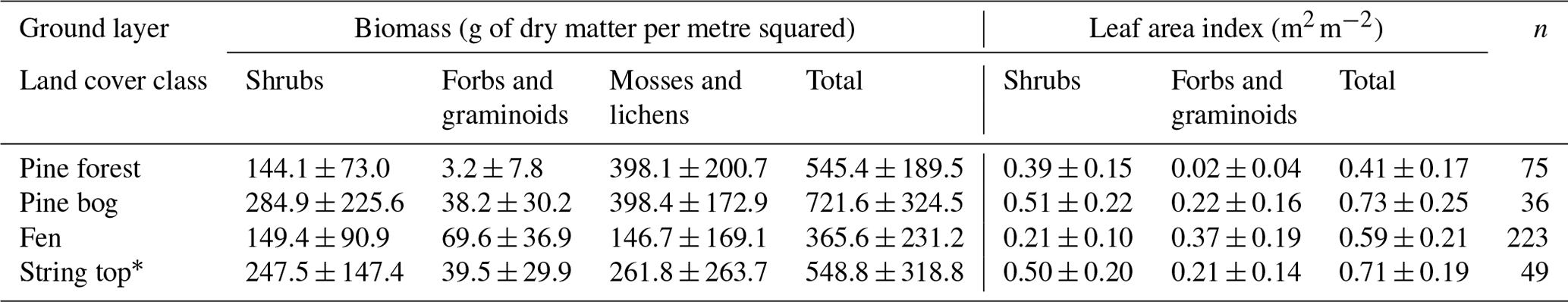
∗ String top CO2 fluxes were used for estimating the ground layer flux of pine bogs.
Table A2Pine forest basal area, stand density, and diameter at breast height (DBH; mean ± standard deviation) derived from field measurements.
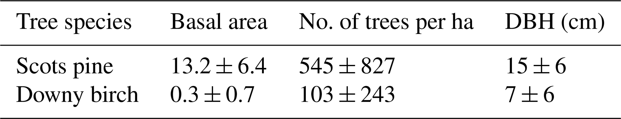
Table A3Average tree height (mean ± standard deviation) and the number of field measurement points.
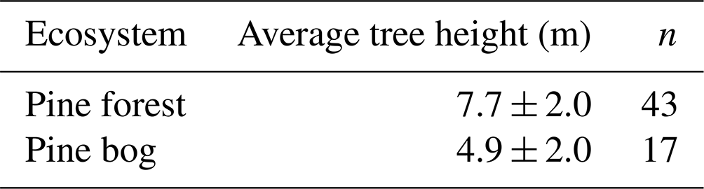
Table A4Soil and peat properties (mean ± standard deviation) for pine forest, pine bog, and fen ecosystems. Except for the pine forest organic layer, pH was always measured at 30 cm depth. In pine bog and fen ecosystems, bulk density, C and N content, and C:N ratio are the mean of 0–5 and 15–20 cm peat layers.

Table A5Tree biomass and leaf area index derived from field and remote sensing measurements.
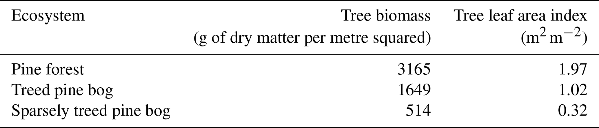
Table A6Annual CO2, CH4, and C balances of the five ecosystems and landscape. Uncertainty estimates were not available for the lake balances (Kou et al., 2022), and thus, they are not taken into account in the landscape-scale uncertainty estimates.
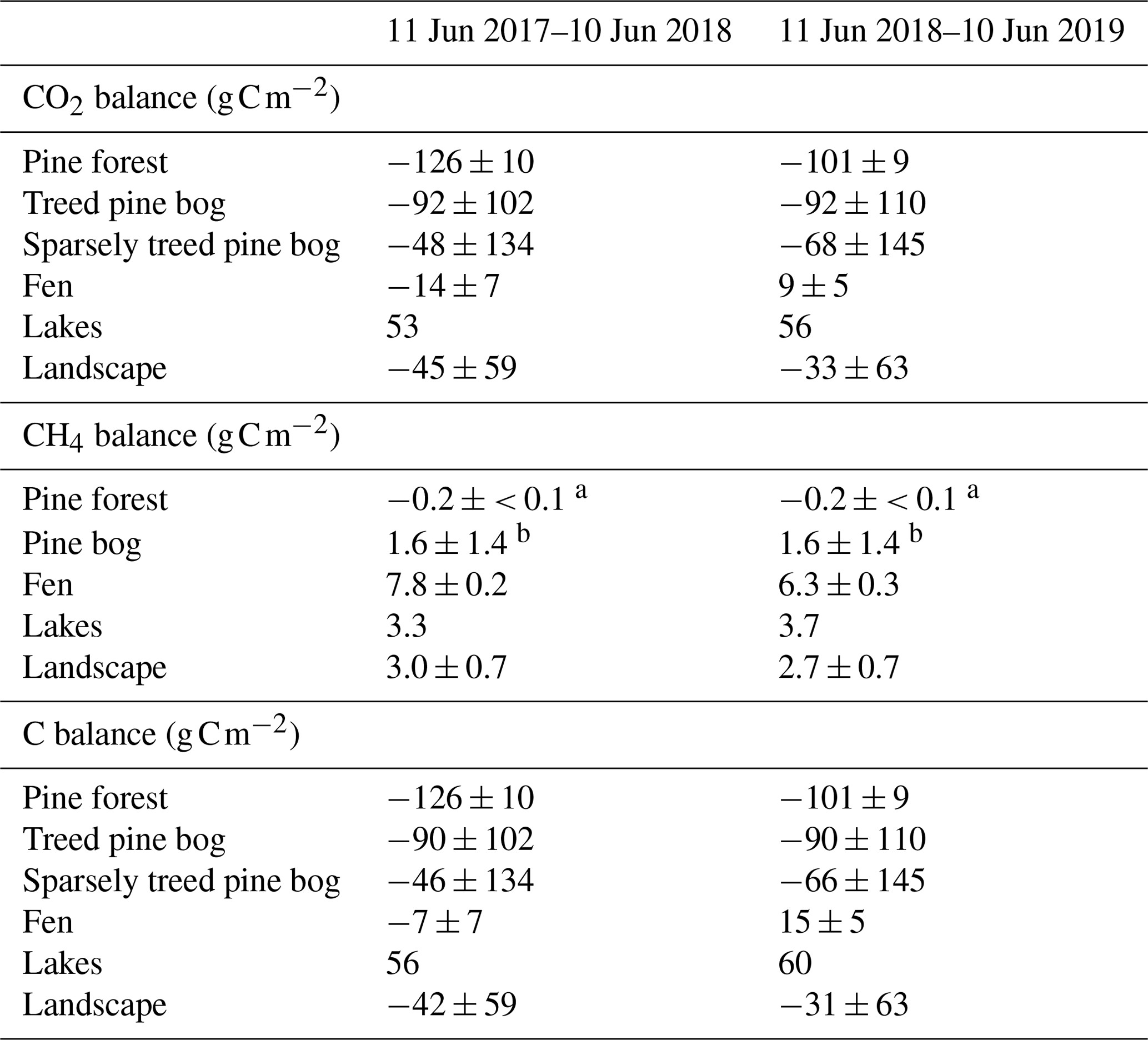
a Dinsmore et al. (2017). b Bubier et al. (2005).
Table A7Data sources for different ecosystems.
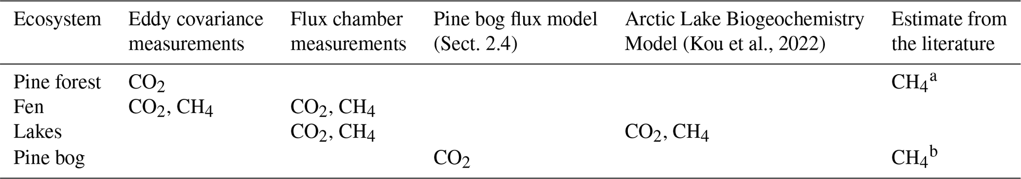
a Dinsmore et al. (2017). b Bubier et al. (2005).
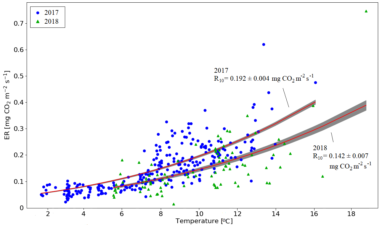
Figure A1Temperature response of ecosystem respiration in the pine forest based on the nighttime EC data for 15 June–15 August 2017 and 2018. The lines show the fitted temperature response , with E0 = 400 K−1 (Lloyd and Taylor, 1994). The shaded areas indicate the one-sigma confidence intervals.
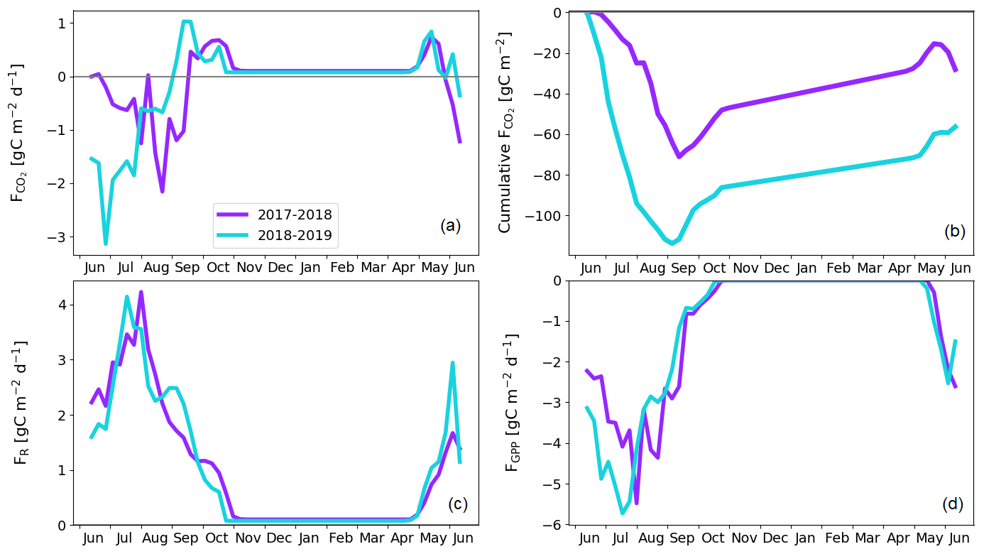
Figure A2String top gap-filled fluxes. Weekly averaged (a) and cumulative CO2 flux (b) and weekly averaged ER (c) and GPP (d) flux, which is used for estimating pine bog ecosystem fluxes.
Table A8Average bulk density, C and N content, and C:N ratio (± standard deviation) in the top 20 cm of lake sediments.
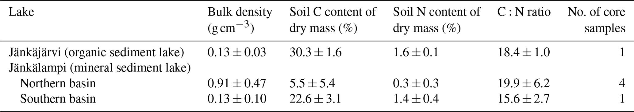
The measured flux and ancillary meteorological and environmental data are available on Zenodo (https://doi.org/10.5281/zenodo.7437333; Heiskanen et al., 2022).
The supplement related to this article is available online at: https://doi.org/10.5194/bg-20-545-2023-supplement.
MA, JPT, and LH designed the study. Terrestrial ecosystem field flux measurements and maintenance were carried out by LH and MA. Aquatic ecosystem field flux measurements were carried out by LH, MA, and SJ. AR, TV, and SJ measured and analysed the vegetation and land cover data. JM measured and analysed the soil data. SJ and LH collected the lake sediment data, and SJ and JM took part in the sediment data analysis. HV was responsible for the eddy covariance data gap-filling and uncertainty analysis. AR and TV conducted the linear regression model analysis. The rest of the data analysis was carried out by LH, JPT, and MA. LH wrote the paper, with contributions from all co-authors.
The contact author has declared that none of the authors has any competing interests.
Publisher's note: Copernicus Publications remains neutral with regard to jurisdictional claims in published maps and institutional affiliations.
We thank Jani Antila, Holtti Hakonen, and Tuuli Lehtosalo, for field assistance, and Jan Weckström and Maija Heikkilä, for granting ancillary lake sediment chemistry data. We thank Dan Kou, for providing the lake flux modelling results. We thank Tuomas Laurila and Timo Penttilä, for expert support on planning the measurement site set-up.
This research has been supported by the Academy of Finland (grant nos. 296888 and 296423) as part of CAPTURE-project and the Maj and Tor Nessling foundation (grant no. 202000391).
This paper was edited by Jamie Shutler and reviewed by two anonymous referees.
Aguadé, D., Poyatos, R., Gómez, M., Oliva, J., and Martínez-Vilalta, J.: The role of defoliation and root rot pathogen infection in driving the mode of drought-related physiological decline in Scots pine (Pinus sylvestris L.), Tree Physiol., 35, 229–242, https://doi.org/10.1093/treephys/tpv005, 2015.
Alm, J., Schulman, L., Walden, J., Nykänen, H., Martikainen, P. J., and Silvola, J.: Carbon Balance of a Boreal Bog during a Year with an Exceptionally Dry Summer, Ecology, 80, 161–174, https://doi.org/10.1890/0012-9658(1999)080[0161:CBOABB]2.0.CO;2, 1999.
Aubinet, M., Vesala, T., and Papale, D.: Eddy Covariance: A Practical Guide to Measurement and Data Analysis, Springer Netherlands, Dordrecht, https://doi.org/10.1007/978-94-007-2351-1, 2012.
Aurela, M., Laurila, T., and Tuovinen, J.-P.: Seasonal CO2 balances of a subarctic mire, J. Geophys. Res.-Atmos., 106, 1623–1637, https://doi.org/10.1029/2000JD900481, 2001.
Aurela, M., Laurila, T., and Tuovinen, J.-P.: Annual CO2 balance of a subarctic fen in northern Europe: Importance of the wintertime efflux, J. Geophys. Res.-Atmos., 107, 4607, https://doi.org/10.1029/2002JD002055, 2002.
Aurela, M., Laurila, T., and Tuovinen, J.-P.: The timing of snow melt controls the annual CO2 balance in a subarctic fen, Geophys. Res. Lett., 31, L16119, https://doi.org/10.1029/2004GL020315, 2004.
Aurela, M., Riutta, T., Laurila, T., Tuovinen, J.-P., Vesala, T., Tuittila, E., Rinne, J., Haapanala, S., and Laine, J.: CO2 exchange of a sedge fen in southern Finland-the impact of a drought period, Tellus B, 59, 826–837, https://doi.org/10.1111/j.1600-0889.2007.00309.x, 2007.
Aurela, M., Lohila, A., Tuovinen, J.-P., Hatakka, J., Penttilä, T., and Laurila, T.: Carbon dioxide and energy flux measurements in four northern-boreal ecosystems at Pallas, Boreal Environ. Res., 20, 455–473, 2015.
Barton, K.: MuMIn: Multi-Model Inference, R package version 1.43.17 [code], https://CRAN.R-project.org/package=MuMIn (last access 1 October 2021), 2020.
Bastviken, D., Cole, J., Pace, M., and Tranvik, L.: Methane emissions from lakes: Dependence of lake characteristics, two regional assessments, and a global estimate, Global Biogeochem. Cy., 18, GB4009, https://doi.org/10.1029/2004GB002238, 2004.
Bond-Lamberty, B., Peckham, S. D., Ahl, D. E., and Gower, S. T.: Fire as the dominant driver of central Canadian boreal forest carbon balance, Nature, 450, 89–92, https://doi.org/10.1038/nature06272, 2007.
Breiman, L.: Random forests, Mach. Learn., 45, 5–32, 2001.
Bubier, J. L., Crill, P. M., Moore, T. R., Savage, K., and Varner, R. K.: Seasonal patterns and controls on net ecosystem CO2 exchange in a boreal peatland complex, Global Biogeochem. Cy., 12, 703–714, https://doi.org/10.1029/98GB02426, 1998.
Bubier, J., Moore, T., Savage, K., and Crill, P.: A comparison of methane flux in a boreal landscape between a dry and a wet year, Global Biogeochem. Cy., 19, GB1023, https://doi.org/10.1029/2004GB002351, 2005.
Büker, P., Morrissey, T., Briolat, A., Falk, R., Simpson, D., Tuovinen, J.-P., Alonso, R., Barth, S., Baumgarten, M., Grulke, N., Karlsson, P. E., King, J., Lagergren, F., Matyssek, R., Nunn, A., Ogaya, R., Peñuelas, J., Rhea, L., Schaub, M., Uddling, J., Werner, W., and Emberson, L. D.: DO3SE modelling of soil moisture to determine ozone flux to forest trees, Atmos. Chem. Phys., 12, 5537–5562, https://doi.org/10.5194/acp-12-5537-2012, 2012.
Chapin, F. S., Matson, P. A., and Vitousek, P.: Principles of Terrestrial Ecosystem Ecology, 2nd Edn., Springer, https://doi.org/10.1007/978-1-4419-9504-9, 2011.
Chen, T. and Guestrin, C.: Xgboost: A scalable tree boosting system, Proceedings of the 22nd ACM SIGKDD international conference on knowledge discovery and data mining, 13–17 August 2016, San Francisco, California, USA, 785–794, 2016.
Chi, J., Nilsson, M. B., Laudon, H., Lindroth, A., Wallerman, J., Fransson, J. E. S., Kljun, N., Lundmark, T., Ottosson Löfvenius, M., and Peichl, M.: The Net Landscape Carbon Balance—Integrating terrestrial and aquatic carbon fluxes in a managed boreal forest landscape in Sweden, Glob. Change Biol., 26, 2353–2367, https://doi.org/10.1111/gcb.14983, 2020.
Cole, J. J., Prairie, Y. T., Caraco, N. F., McDowell, W. H., Tranvik, L. J., Striegl, R. G., Duarte, C. M., Kortelainen, P., Downing, J. A., Middelburg, J. J., and Melack, J.: Plumbing the global carbon cycle: Integrating inland waters into the terrestrial carbon budget, Ecosystems, 10, 171–184, https://doi.org/10.1007/s10021-006-9013-8, 2007.
Denfeld, B. A., Lupon, A., Sponseller, R. A., Laudon, H., and Karlsson, J.: Heterogeneous CO2 and CH4 patterns across space and time in a small boreal lake, Inland Waters, 10, 348–359, https://doi.org/10.1080/20442041.2020.1787765, 2020.
Deppe, M., Knorr, K.-H., McKnight, D. M., and Blodau, C.: Effects of short-term drying and irrigation on CO2 and CH4 production and emission from mesocosms of a northern bog and an alpine fen, Biogeochemistry, 100, 89–103, https://doi.org/10.1007/s10533-010-9406-9, 2010.
Dinsmore, K. J., Drewer, J., Levy, P. E., George, C., Lohila, A., Aurela, M., and Skiba, U. M.: Growing season CH4 and N2O fluxes from a subarctic landscape in northern Finland; from chamber to landscape scale, Biogeosciences, 14, 799–815, https://doi.org/10.5194/bg-14-799-2017, 2017.
Du, Y., Wang, Y., Su, F., Jiang, J., Wang, C., Yu, M., and Yan, J.: The response of soil respiration to precipitation change is asymmetric and differs between grasslands and forests, Glob. Change Biol., 26, 6015–6024, https://doi.org/10.1111/gcb.15270, 2020.
Foken, T. and Wichura, B.: Tools for quality assessment of surface-based flux measurements, Agr. Forest Meteorol., 78, 83–105, https://doi.org/10.1016/0168-1923(95)02248-1, 1996.
Fronzek, S., Carter, T., Räisänen, J., Ruokolainen, L., and Luoto, M.: Applying probabilistic projections of climate change with impact models: A case study for sub-arctic palsa mires in Fennoscandia, Climatic Change, 99, 515–534, https://doi.org/10.1007/s10584-009-9679-y, 2010.
Gao, Y., Markkanen, T., Aurela, M., Mammarella, I., Thum, T., Tsuruta, A., Yang, H., and Aalto, T.: Response of water use efficiency to summer drought in a boreal Scots pine forest in Finland, Biogeosciences, 14, 4409–4422, https://doi.org/10.5194/bg-14-4409-2017, 2017.
Guo, M., Zhuang, Q., Tan, Z., Shurpali, N., Juutinen, S., Kortelainen, P., and Martikainen, P. J.: Rising methane emissions from boreal lakes due to increasing ice-free days, Environ. Res. Lett., 15, 064008, https://doi.org/10.1088/1748-9326/ab8254, 2020.
Hadden, D. and Grelle, A.: Net CO2 emissions from a primary boreo-nemoral forest over a 10 year period, Forest Ecol. Manag., 398, 164–173, https://doi.org/10.1016/j.foreco.2017.05.008, 2017.
Hargreaves, K. J., Fowler, D., Pitcairn, C. E. R., and Aurela, M.: Annual methane emission from Finnish mires estimated from eddy covariance campaign measurements, Theor. Appl. Climatol., 70, 203–213, https://doi.org/10.1007/s007040170015, 2001.
Heiskanen, L., Tuovinen, J.-P., Räsänen, A., Virtanen, T., Juutinen, S., Lohila, A., Penttilä, T., Linkosalmi, M., Mikola, J., Laurila, T., and Aurela, M.: Carbon dioxide and methane exchange of a patterned subarctic fen during two contrasting growing seasons, Biogeosciences, 18, 873–896, https://doi.org/10.5194/bg-18-873-2021, 2021.
Heiskanen, L., Tuovinen, J-P., Vekuri, H., Räsänen, A., Virtanen, T., Juutinen, S., Lohila, A., Mikola, J., and Aurela, M.: Meteorological responses of carbon dioxide and methane fluxes in the terrestrial and aquatic ecosystems of a subarctic landscape (Version v2), Zenodo [data set], https://doi.org/10.5281/zenodo.7437333, 2022.
Irvin, J., Zhou, S., McNicol, G., Lu, F., Liu, V., Fluet-Chouinard, E., Ouyang, Z., Knox, S. H., Lucas-Moffat, A., Trotta, C., Papale, D., Vitale, D., Mammarella, I., Alekseychik, P., Aurela, M., Avati, A., Baldocchi, D., Bansal, S., Bohrer, G., Campbell, D. I., Chen, J., Chu, H., Dalmagro, H. J., Delwiche, K. B., Desai, A. R., Euskirchen, E., Feron, S., Goeckede, M., Heimann, M., Helbig, M., Helfter, C., Hemes, K. S., Hirano, T., Iwata, H., Jurasinski, G., Kalhori, A., Kondrich, A., Lai, D. Y. F., Lohila, A., Malhotra, A., Merbold, L., Mitra, B., Ng, A., Nilsson, M. B., Noormets, A., Peichl, M., Rey-Sanchez, A. C., Richardson, A. D., Runkle, B. R. K., Schäfer, K. V. R., Sonnentag, O., Stuart-Haëntjens, E., Sturtevant, C., Ueyama, M., Valach, A. C., Vargas, R., Vourlitis, G. L., Ward, E. J., Xhuan Wong, G., Zona, D., Alberto, Ma, C. R., Billesbach, D. P., Celis, G., Dolman, H., Friborg, T., Fuchs, K., Gogo, S., Gondwe, M. J., Goodrich, J. P., Gottschalk, P., Hörtnagl, L., Jacotot, A., Koebsch, F., Kasak, K., Maier, R., Morin, T. H., Nemitz, E., Oechel, W. C., Oikawa, P. Y., Ono, K., Sachs, T., Sakabe, A., Schuur, E. A., Shortt, R., Sullivan, R. C., Szutu, D. J., Tuittila, E.-S., Varlagin, A., Verfaillie, J. G., Wille, C., Windham-Myers, L., Poulter, B., and Jackson, R. B.: Gap-filling eddy covariance methane fluxes: Comparison of machine learning model predictions and uncertainties at FLUXNET-CH4 wetlands, Agr. Forest Meteorol., 308, 108528, https://doi.org/10.1016/j.agrformet.2021.108528, 2021.
Jammet, M., Dengel, S., Kettner, E., Parmentier, F.-J. W., Wik, M., Crill, P., and Friborg, T.: Year-round CH4 and CO2 flux dynamics in two contrasting freshwater ecosystems of the subarctic, Biogeosciences, 14, 5189–5216, https://doi.org/10.5194/bg-14-5189-2017, 2017.
Jansen, J., Thornton, B. F., Cortés, A., Snöälv, J., Wik, M., MacIntyre, S., and Crill, P. M.: Drivers of diffusive CH4 emissions from shallow subarctic lakes on daily to multi-year timescales, Biogeosciences, 17, 1911–1932, https://doi.org/10.5194/bg-17-1911-2020, 2020.
Jones, H. G.: Plants and Microclimate: A Quantitative Approach to Environmental Plant Physiology, Cambridge University Press, West Nyack, https://doi.org/10.1017/CBO9780511845727, 2013.
Juutinen, S., Väliranta, M., Kuutti, V., Laine, A. M., Virtanen, T., Seppä, H., Weckström, J., and Tuittila, E-S.: Short-term and long-term carbon dynamics in a northern peatland-stream-lake continuum: A catchment approach, J. Geophys. Res.-Biogeo., 118, 171–183, https://doi.org/10.1002/jgrg.20028, 2013.
Kätterer, T., Reichstein, M., Andrén, O., and Lomander, A.: Temperature dependence of organic matter decomposition: a critical review using literature data analyzed with different models, Biol. Fert. Soils, 27, 258–262, https://doi.org/10.1007/s003740050430, 1998.
Kljun, N., Black, T. A., Griffis, T. J., Barr, A. G., Gaumont-Guay, D., Morgenstern, K., McCaughey, J. H., and Nesic, Z.: Response of net ecosystem productivity of three boreal forest stands to drought, Ecosystems, 10, 1039–1055, https://doi.org/10.1007/s10021-007-9088-x, 2007.
Kortelainen, P., Rantakari, M., Huttunen, J. T., Mattsson, T., Alm, J., Juutinen, S., Larmola, T., Silvola, J., and Martikainen, P. J.: Sediment respiration and lake trophic state are important predictors of large CO2 evasion from small boreal lakes, Glob. Change Biol., 12, 1554–1567, https://doi.org/10.1111/j.1365-2486.2006.01167.x, 2006.
Kou, D., Virtanen, T., Treat, C. C., Tuovinen, J.-P., Räsänen, A., Juutinen, S., Mikola, J., Aurela, M., Heiskanen, L., Heikkilä, M., Weckström, J., Juselius, T., Piilo, S. R., Deng, J., Zhang, Y., Chaudhary, N., Huang, C., Väliranta, M., Biasi, C., Liu, X., Guo, M., Zhuang, Q., Korhola, A., and Shurpali, N. J.: Peatland heterogeneity impacts on regional carbon flux and its radiative effect within a boreal landscape, J. Geophys. Res.-Biogeo., 127, e2021JG006774, https://doi.org/10.1029/2021JG006774, 2022.
Kulmala, L., Pumpanen, J., Kolari, P., Dengel, S., Berninger, F., Köster, K., Matkala, L., Vanhatalo, A., Vesala, T., and Bäck, J.: Inter- and intra-annual dynamics of photosynthesis differ between forest floor vegetation and tree canopy in a subarctic Scots pine stand, Agr. Forest Meteorol., 271, 1–11, 2019.
Laurila, T., Soegaard, H., Lloyd, C. R., Aurela, M., Tuovinen, J.-P., and Nordstroem, C.: Seasonal variations of net CO2 exchange in European Arctic ecosystems, Theor. Appl. Climatol., 70, 183–201, https://doi.org/10.1007/s007040170014, 2001.
Laurila, T., Tuovinen, J.-P., Lohila, A., Hatakka, J., Aurela, M., Thum, T., Pihlatie, M., Rinne, J., and Vesala, T.: Measuring methane emissions from a landfill using a cost effective micrometeorological method, Geophys. Res. Lett., 32, LI9808, https://doi.org/10.1029/2005GL023462, 2005.
Le Mer, J. and Roger, P.: Production, oxidation, emission and consumption of methane by soils: A review, Eur. J. Soil Biol., 37, 25–50, https://doi.org/10.1016/S1164-5563(01)01067-6, 2001.
Lehtonen, I. and Pirinen, P.: 2018: An exceptionally warm thermal growing season in Finland, in: FMI's Climate Bulletin: Research Letters, Finnish Meteorological Institute, Helsinki, https://doi.org/10.35614/ISSN-2341-6408-IK-2019-03-RL, 2019a.
Lehtonen, I. and Pirinen, P.: 2018: An exceptionally dry thermal growing season in Finland, in: FMI's Climate Bulletin: Research Letters, Finnish Meteorological Institute, Helsinki, https://doi.org/10.35614/ISSN-2341-6408-IK-2019-04-RL, 2019b.
Lindroth, A., Lund, M., Nilsson, M., Aurela, M., Christensen, T. R., Laurila, T., Rinne, J., Riutta, T., Sagerfors, J., StröM, L., Tuovinen, J., and Vesala, T.: Environmental controls on the CO2 exchange in north European mires, Tellus B, 59, 812–825, https://doi.org/10.1111/j.1600-0889.2007.00310.x, 2007.
Lindroth, A., Lagergren, F., Aurela, M., Bjarnadottir, B., Christensen, T., Dellwik, E., Grelle, A., Ibrom, A., Johansson, T., Lankreijer, H., Launiainen, S., Laurila, T., Mölder, M., Nikinmaa, E., Pilegaard, K., Sigurdsson, B. D., and Vesala, T.: Leaf area index is the principal scaling parameter for both gross photosynthesis and ecosystem respiration of Northern deciduous and coniferous forests, Tellus B, 60, 129–142, https://doi.org/10.3402/tellusb.v60i2.16909, 2008.
Lindroth, A., Holst, J., Linderson, M., Aurela, M., Biermann, T., Heliasz, M., Chi, J., Ibrom, A., Kolari, P., Klemedtsson, L., Krasnova, A., Laurila, T., Lehner, I., Lohila, A., Mammarella, I., Mölder, M., Löfvenius, M. O., Peichl, M., Pilegaard, K., Soosar, K., Vesala, T., Vestin, P., Weslien, P., and Nilsson, M.: Effects of drought and meteorological forcing on carbon and water fluxes in Nordic forests during the dry summer of 2018, Philos. T. R. Soc. Lon. B, 375, 20190516, https://doi.org/10.1098/rstb.2019.0516, 2020.
Linkosalmi, M., Tuovinen, J.-P., Nevalainen, O., Peltoniemi, M., Taniş, C. M., Arslan, A. N., Rainne, J., Lohila, A., Laurila, T., and Aurela, M.: Tracking vegetation phenology of pristine northern boreal peatlands by combining digital photography with CO2 flux and remote sensing data, Biogeosciences, 19, 4747–4765, https://doi.org/10.5194/bg-19-4747-2022, 2022.
Lloyd, J. and Taylor, J. A.: On the Temperature Dependence of Soil Respiration, Funct. Ecol., 8, 315–323, https://doi.org/10.2307/2389824, 1994.
Lohila, A., Tuovinen, J.-P., Hatakka, J., Aurela, M., Vuorenmaa, J., Haakana, M., and Laurila, T.: Carbon dioxide and energy fluxes over a northern boreal lake, Boreal Environ. Res., 20, 474–488, 2015.
López Bellido, J., Tulonen, T., Kankaala, P., and Ojala, A.: CO2 and CH4 fluxes during spring and autumn mixing periods in a boreal lake (Pääjärvi, southern Finland), J. Geophys. Res., 114, G04007, https://doi.org/10.1029/2009jg000923, 2009.
Maanavilja, L., Riutta, T., Aurela, M., Laurila, T., and Tuittila, E.-S.: Spatial variation in CO2 exchange at a northern aapa mire, Biogeochemistry, 104, 325–345, https://doi.org/10.1007/s10533-010-9505-7, 2011.
Martín-Gómez, P., Aguilera, M., Pemán, J., Gil-Pelegrín, E., and Ferrio, J. P.: Contrasting ecophysiological strategies related to drought: the case of a mixed stand of Scots pine (Pinus sylvestris) and a submediterranean oak (Quercus subpyrenaica), Tree Physiol., 37, 1478–1492, https://doi.org/10.1093/treephys/tpx101, 2017.
Masson-Delmotte, V., Zhai, P., Pörtner, H.-O., Roberts, D., Skea, J., Shukla, P. R., Pirani, A., Moufouma-Okia, W., Péan, C., Pidcock, R., Connors, S., Matthews, J. B. R., Chen, Y., Zhou, X., Gomis, M. I., Lonnoy, E., Maycock, T., Tignor, M., and Waterfield, T. (Eds.): Global Warming of 1.5 ∘C. An IPCC Special Report on the impacts of global warming of 1.5 ∘C above pre-industrial levels and related global greenhouse gas emission pathways, in the context of strengthening the global response to the threat of climate change, sustainable development, and efforts to eradicate poverty, World Meteorological Organization, Geneva, Switzerland, https://doi.org/10.1017/9781009157940, 2018.
Matkala, L., Kulmala, L., Kolari, P., Aurela, M., and Bäck, J.: Resilience of subarctic Scots pine and Norway spruce forests to extreme weather events. Agr. Forest Meteorol., 296, 108239, https://doi.org/10.1016/j.agrformet.2020.108239, 2021.
McElligott, K. M., Seiler, J. R., and Strahm, B. D.: The Impact of Water Content on Sources of Heterotrophic Soil Respiration, Forests, 8, 299, https://doi.org/10.3390/f8080299, 2017.
McMillen, R. T.: An eddy correlation technique with extended applicability to non-simple terrain, Bound.-Lay. Meteorol., 43, 231–245, https://doi.org/10.1007/BF00128405, 1988.
Mekonnen, Z. A., Riley, W. J., Berner, L. T., Bouskill, N. J., Torn, M. S., Iwahana, G., Breen, A. L., Myers-Smith, I. H., García Criado, M., Liu, Y., Euskirchen, E. S., Goetz, S. J., Mack, M. C., and Grant, R. F.: Arctic tundra shrubification: a review of mechanisms and impacts on ecosystem carbon balance, Environ. Res. Lett., 16, 053001, https://doi.org/10.1088/1748-9326/abf28b, 2021.
Meyer, N., Welp, G., and Amelung, W.: The temperature sensitivity (Q10) of soil respiration: controlling factors and spatial prediction at regional scale based on environmental soil classes, Global Biogeochem. Cyc., 32, 306–323, https://doi.org/10.1002/2017GB005644, 2018.
Montagnani, L., Grünwald, T., Kowalski, A., Mammarella, I., Merbold, L., Metzger, S., Sedlák, P., and Siebicke, L.: Estimating the storage term in eddy covariance measurements: the ICOS methodology, Int. Agrophys., 32, 551–567, https://doi.org/10.1515/intag-2017-0037, 2018.
Moyano, F. E., Vasilyeva, N., Bouckaert, L., Cook, F., Craine, J., Curiel Yuste, J., Don, A., Epron, D., Formanek, P., Franzluebbers, A., Ilstedt, U., Kätterer, T., Orchard, V., Reichstein, M., Rey, A., Ruamps, L., Subke, J.-A., Thomsen, I. K., and Chenu, C.: The moisture response of soil heterotrophic respiration: interaction with soil properties, Biogeosciences, 9, 1173–1182, https://doi.org/10.5194/bg-9-1173-2012, 2012.
Muilu-Mäkelä, R., Vuosku, J., Läärä, E., Saarinen, M., Heiskanen, J., Häggman, H., and Sarjala, T.: Water availability influences morphology, mycorrhizal associations, PSII efficiency and polyamine metabolism at early growth phase of Scots pine seedlings, Plant Physiol. Bioch., 88, 70–81, https://doi.org/10.1016/j.plaphy.2015.01.009, 2015.
Neubauer, S. C.: Global Warming Potential Is Not an Ecosystem Property, Ecosystems, 24, 2079–2089, https://doi.org/10.1007/s10021-021-00631-x, 2021.
Neubauer, S. C. and Megonigal, J. P.: Moving Beyond Global Warming Potentials to Quantify the Climatic Role of Ecosystems, Ecosystems, 18, 1000–1013, https://doi.org/10.1007/s10021-015-9879-4, 2015.
Orchard, V. A. and Cook, F. J.: Relationship between soil respiration and soil moisture, Soil Biol. Biochem., 15, 447–453, 1983.
Piilo, S. R., Korhola, A., Heiskanen, L., Tuovinen, J.-P., Aurela, M., Juutinen, S., Marttila, H., Saari, M., Tuittila, E.-S., Turunen, J., and Väliranta, M. M.: Spatially varying peatland initiation, Holocene development and estimated radiative forcing within a subarctic fen, Quaternary Sci. Rev., 248, 106596, https://doi.org/10.1016/j.quascirev.2020.106596, 2020.
Pirinen, P., Simola, H., Aalto, J., Kaukoranta, J.-P., Karlsson, P., and Ruuhela, R.: Climatological Statistics of Finland 1981–2010, Reports 2012:1, Finnish Meteorological Institute, Helsinki, Finland, 2012.
R Core Team: R: A language and environment for statistical computing, R Foundation for Statistical Computing [code], Vienna, Austria, https://www.R-project.org, last access: 1 October 2021.
Räsänen, A. and Virtanen, T.: Data and resolution requirements in mapping vegetation in spatially heterogeneous landscapes, Remote Sens. Environ., 230, 111207, https://doi.org/10.1016/j.rse.2019.05.026, 2019.
Räsänen, A., Juutinen, S., Tuittila, E-S., Aurela, M., and Virtanen, T.: Comparing ultra-high spatial resolution remote-sensing methods in mapping peatland vegetation, J. Veg. Sci., 30, 1016–1026, https://doi.org/10.1111/jvs.12769, 2019.
Rasilo, T., Prairie, Y. T., and del Giorgio, P. A.: Large-scale patterns in summer diffusive CH4 fluxes across boreal lakes, and contribution to diffusive C emissions, Glob. Change Biol., 21, 1124–1139, https://doi.org/10.1111/gcb.12741, 2015.
Richardson, A. D., Mahecha, M. D., Falge, E., Kattge, J., Moffat, A. M., Papale, D., Reichstein, M., Stauch, V. J., Braswell, B. H., Churkina, G., Kruijt, B., and Hollinger, D. Y.: Statistical properties of random CO2 flux measurement uncertainty inferred from model residuals, Agr. Forest Meteorol., 148, 38–50, 2008.
Rinne, J., Tuovinen, J.-P., Klemedtsson, L., Aurela, M., Holst, J., Lohila, A., Weslien, P., Vestin, P., Łakomiec, P., Peichl, M., Tuittila, E.-S., Heiskanen, L., Laurila, T., Li, X., Alekseychik, P., Mammarella, I., Ström, L., Crill, P., and Nilsson, M. B.: Effect of the 2018 European drought on methane and carbon dioxide exchange of northern mire ecosystems, Philos. T. R. Soc., 375, B37520190517, https://doi.org/10.1098/rstb.2019.0517, 2020.
Sagerfors, J., Lindroth, A., Grelle, A., Klemedtsson, L., Weslien, P., and Nilsson, M.: Annual CO2 exchange between a nutrient-poor, minerotrophic, boreal mire and the atmosphere, J. Geophys. Res., 113, G01001, https://doi.org/10.1029/2006JG000306, 2008.
Sepulveda-Jauregui, A., Walter Anthony, K. M., Martinez-Cruz, K., Greene, S., and Thalasso, F.: Methane and carbon dioxide emissions from 40 lakes along a north–south latitudinal transect in Alaska, Biogeosciences, 12, 3197–3223, https://doi.org/10.5194/bg-12-3197-2015, 2015.
Silfver, T., Heiskanen, L., Aurela, M., Myller, K., Karhu, K., Meyer, N., Tuovinen, J-P., Oksanen, E., Rousi, M., and Mikola, J.: Insect herbivory dampens subarctic birch forest C sink response to warming, Nat. Commun. 11, 2529, https://doi.org/10.1038/s41467-020-16404-4, 2020.
Strack, M. and Waddington, J. M.: Response of peatland carbon dioxide and methane fluxes to a water table drawdown experiment, Global Biogeochem. Cy., 21, GB1007, https://doi.org/10.1029/2006GB002715, 2007.
Tan, Z., Zhuang, Q., and Anthony, K. W.: Modeling methane emissions from arctic lakes: Model development and site-level study, J. Adv. Model. Earth Sy., 7, 459–483, https://doi.org/10.1002/2014ms000344, 2015.
Tan, Z., Zhuang, Q., Shurpali, N. J., Marushchak, M. E., Biasi, C., Eugster, W., and Anthony, K. W.: Modeling CO2 emissions from Arctic lakes: Model development and site-level study. J. Adv. Model. Earth Sy., 9, 2190–2213 https://doi.org/10.1002/2017ms001028, 2017.
Thornton, B. F., Wik, M., and Crill, P. M.: Climate-forced changes in available energy and methane bubbling from subarctic lakes, Geophys. Res. Lett., 42, 1936–1942, https://doi.org/10.1002/2015GL063189, 2015.
Tranvik, L. J., Downing, J. A., Cotner, J. B., Loiselle, S. A., Striegl, R. G., Ballatore, T. J., Dillon, P., Knoll, L. B., Kutser, T., Larsen, S., Laurion, I., Leech, D. M., McAllister, S. L., McKnight, D. M., Melack, J., Overholt, E., Porter, J. A., Prairie, Y. T., Renwick, W. H., Roland, F., Sherman, B. S., Schindler, D. W., Sobek, S., Tremblay, A., Vanni, M. J., Verschoor, A. M., von Wachenfeldt, E., and Weyhenmeyer, G.: Lakes and Reservoirs as Regulators of Carbon Cycling and Climate, Limnol. Oceanogr., 54, 2298–2314, https://doi.org/10.4319/lo.2009.54.6_part_2.2298, 2009.
Venables, W. N. and Ripley, B. D.: Modern Applied Statistics with S, 4th Edn., Springer, New York, https://doi.org/10.1007/978-0-387-21706-2, 2002.
Vicente-Serrano, S., Begueria, S., and Lopez-Moreno, J.: A Multiscalar Drought Index Sensitive to Global Warming: The Standardized Precipitation Evapotranspiration Index, J. Climate, 23, 1696–1718, https://doi.org/10.1175/2009JCLI2909.1, 2010.
Virkkala, A. M., Aalto, J., Rogers, B. M., Tagesson, T., Treat, C. C., Natali, S. M., Watts, J. D., Potter, S., Lehtonen, A., Mauritz, M., Schuur, E. A. G., Kochendorfer, J., Zona, D., Oechel, W., Kobayashi, H., Humphreys, E., Goeckede, M., Iwata, H., Lafleur, P. M., Euskirchen, E. S., Bokhorst, S., Marushchak, M., Martikainen, P. J., Elberling, B., Voigt, C., Biasi, C., Sonnentag, O., Parmentier, F.-J. W., Ueyama, M., Celis, G., St. Louis, V. L., Emmerton, C. A., Peichl, M., Chi, J., Järveoja, J., Nilsson, M. B., Oberbauer, S. F., Torn, M. S., Park, S. J., Dolman, H., Mammarella, I., Chae, N., Poyatos, R., López-Blanco, E., Christensen, T. R., Kwon, M. J., Sachs, T., Holl, D., and Luoto, M.: Statistical upscaling of ecosystem CO2 fluxes across the terrestrial tundra and boreal domain: Regional patterns and uncertainties, Glob. Change Biol., 27, 4040–4059, https://doi.org/10.1111/gcb.15659, 2021.
Walter, K. M., Zimov, S. A., Chanton, J. P., Verbyla, D., and Chapin III, F. S.: Methane bubbling from Siberian thaw lakes as a positive feedback to climate warming, Nature, 443, 71–75, https://doi.org/10.1038/nature05040, 2006.
White, J. R., Shannon, R. D., Weltzin, J. F., Pastor, J., and Bridgham, S. D.: Effects of soil warming and drying on methane cycling in a northern peatland mesocosm study, J. Geophys. Res.-Biogeo., 113, G00A06, https://doi.org/10.1029/2007JG000609, 2008.
Whiting, G. J.: CO2 exchange in the Hudson Bay lowlands: Community characteristics and multispectral reflectance properties, J. Geophys. Res., 99, 1519–1528, https://doi.org/10.1029/93JD01833, 1994.
Wik, M., Crill, P. M., Varner, R. K., and Bastviken, D.: Multiyear measurements of ebullitive methane flux from three subarctic lakes, J. Geophys. Res.-Biogeo., 118, 1307–1321, https://doi.org/10.1002/jgrg.20103, 2013.
Wik, M., Johnson, J. E., Crill, P. M., DeStasio, J. P., Erickson, L., Halloran, M. J., Fahnestock, M. F., Crawford, M. K., Phillips, S. C., and Varner, R. K.: Sediment Characteristics and Methane Ebullition in Three Subarctic Lakes, Journal of geophysical research, Biogeosciences, 123, 2399–2411, https://doi.org/10.1029/2017JG004298, 2018.
Zhu, S., Clement, R., McCalmont, J., Davies, C. A., and Hill, T.: Stable gap-filling for longer eddy covariance data gaps: A globally validated machine-learning approach for carbon dioxide, water, and energy fluxes, Agr. Forest Meteorol., 314, 108777, https://doi.org/10.1016/j.agrformet.2021.108777, 2022.