the Creative Commons Attribution 4.0 License.
the Creative Commons Attribution 4.0 License.
 | 07 Mar 2024
Linking northeastern North Pacific oxygen changes to upstream surface outcrop variations
Kyla Drushka
Understanding the response of the ocean to global warming, including the renewal of ocean waters from the surface (ventilation), is important for future climate predictions. Oxygen distributions in the ocean thermocline have proven an effective way to infer changes in ventilation because physical processes (ventilation and circulation) that supply oxygen are thought to be primarily responsible for changes in interior oxygen concentrations. Here, the focus is on the North Pacific thermocline, where some of the world's oceans' largest oxygen variations have been observed. These variations, described as bi-decadal cycles on top of a small declining trend, are strongest on subsurface isopycnals that outcrop into the mixed layer of the northwestern North Pacific in late winter. In this study, surface density time series are reconstructed in this area using observational data only and focusing on the time period from 1982, the first full year of the satellite sea surface temperature record, to 2020. It is found that changes in the annual maximum outcrop area of the densest isopycnals outcropping in the northwestern North Pacific are correlated with interannual oxygen variability observed at Ocean Station P (OSP) downstream at about a 10-year lag. The hypothesis is that ocean ventilation and uptake of oxygen is greatly reduced when the outcrop areas are small and that this signal travels within the North Pacific Current to OSP, with 10 years being at the higher end of transit times reported in other studies. It is also found that sea surface salinity (SSS) dominates over sea surface temperature (SST) in driving interannual fluctuations in annual maximum surface density in the northwestern North Pacific, highlighting the role that salinity may play in altering ocean ventilation. In contrast, SSS and SST contribute about equally to the long-term declining surface density trends that are superimposed on the interannual cycles.
- Article
(7325 KB) - Full-text XML
- BibTeX
- EndNote


Ventilation, the renewal of ocean waters from the sea surface, is expected to decrease due to ocean warming and the resulting increases in stratification (Helm et al., 2011; Capotondi et al., 2012; Heinze et al., 2015). During ventilation, water that is transported from the surface mixed layer into the ocean interior also carries along atmospheric gases, including oxygen (O2) and carbon dioxide (CO2), that have been exchanged between the ocean and the atmosphere while the water was at the surface. A reduction in ventilation has thus also been linked to deoxygenation in the ocean interior (Keeling et al., 2010) and reduced uptake of anthropogenic CO2 (Heinze et al., 2015; Franco et al., 2021) by the world's oceans. This has impacts on ocean ecosystems because a reduction in O2 can shift previously well-oxygenated marine environments to hypoxic conditions (Whitney et al., 2007), affecting marine life. A reduction in oceanic CO2 uptake creates a positive feedback to global warming caused by rising atmospheric CO2 levels, since it leaves more CO2 in the atmosphere (Friedlingstein, 2015).
The North Pacific thermocline is one of the first regions for which large variations in oceanic O2 concentrations were observed and linked to ventilation changes (Andreev and Kusakabe, 2001; Emerson et al., 2001; Ono et al., 2001; Watanabe et al., 2001; Emerson et al., 2004). Observations from repeat hydrographic sections have shown that O2 changes between decades can be 20 µmol kg−1 or more in both the eastern and western North Pacific (Mecking et al., 2008; Takatani et al., 2012; Sasano et al., 2015). Time series data taken over 50 years from Ocean Station P (OSP; 145° W, 50° N) in the Gulf of Alaska in the northeastern North Pacific (black circles in Fig. 1) have indicated that there are bi-decadal O2 variations that occur on subsurface isopycnals in addition to a smaller declining trend associated with ocean warming (Whitney et al., 2007; Cummins and Ross, 2020). Similar variations (of opposite sign) are found to occur at OSP in dissolved inorganic carbon (DIC) and nutrients (Whitney et al., 2007; Franco et al., 2021), since O2 consumption and nutrient/DIC production are linked to each other through stoichiometric ratios during the remineralization of organic matter (Anderson and Sarmiento, 1994). The bi-decadal cycles in the Gulf of Alaska roughly correspond to oscillations in O2 and nutrients observed in the western subarctic North Pacific (Ono et al., 2001) with an order 5–10-year lag depending on the density surface (Whitney et al., 2007), likely reflecting the time that it takes for waters formed in the northwestern North Pacific to travel east with the North Pacific Current.
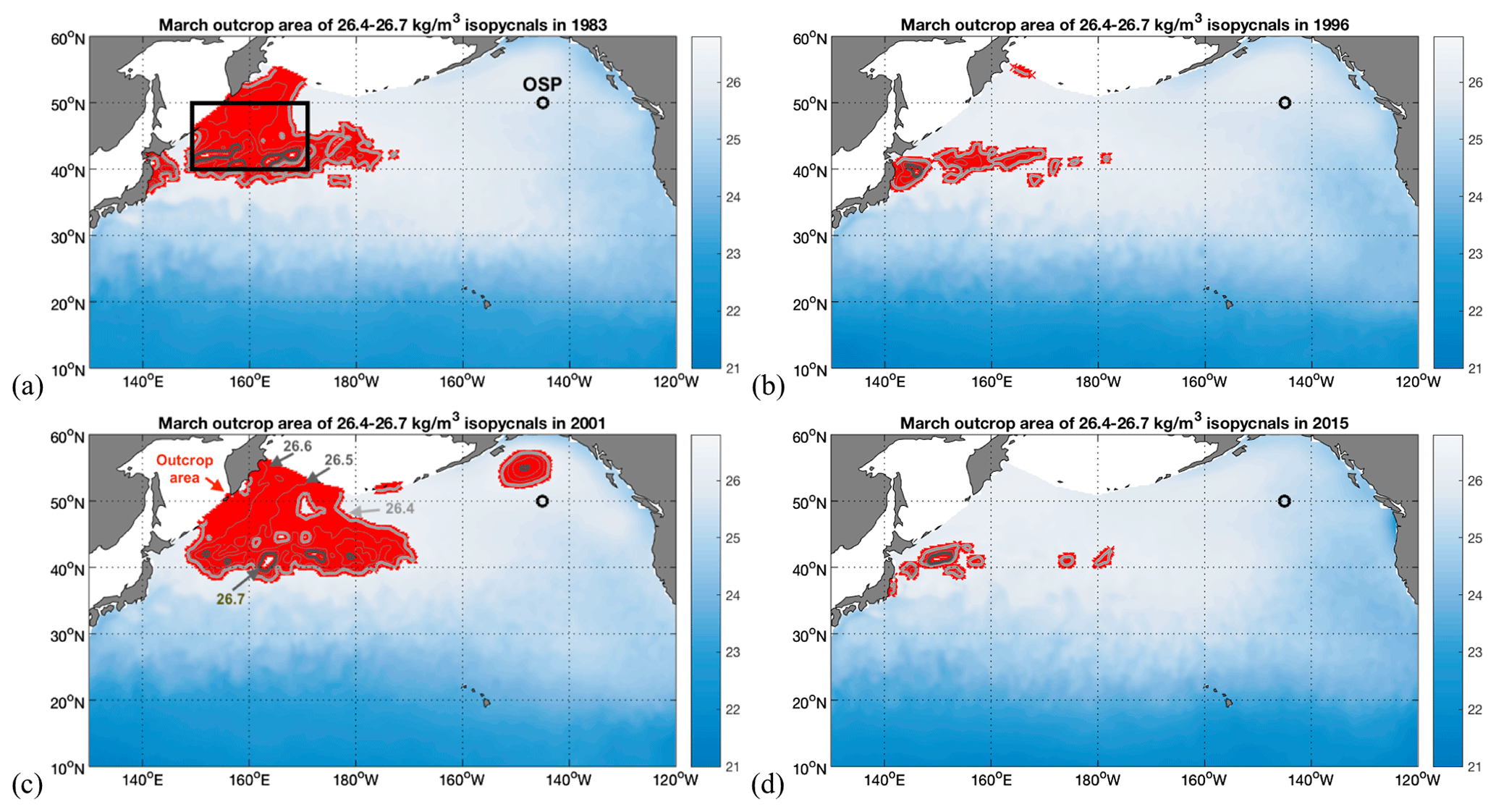
Figure 1Examples of maxima (a, c) and minima (b, d) of March outcrop areas of the σθ = 26.4–26.7 kg m−3 isopycnal range: (a) 1983, (b) 1996, (c) 2001, and (d) 2015. The dataset used is EN4-OISST: ° satellite SST combined with EN4 SSS (interpolated to °; see text). The color shading and color bar show surface potential density anomalies, with anomalies in the σθ = 26.4–26.7 kg m−3 range indicated with red markers, highlighting the outcrop area of this isopycnal range as labeled in (c). Contour lines, as labeled in (c), show the σθ = 26.4 kg m−3 (bold light-gray line), σθ=26.5 kg m−3 and σθ = 26.6 kg m−3 (thin medium-gray lines), and σθ = 26.7 kg m−3 (bold dark-gray line) outcrops. The location of OSP at 50° N, 145° W, as labeled in (a), is marked by an open black circle. The area used for northwestern North Pacific SST, SSS, and surface density averaging (as shown in Figs. 6, A1, A8, A9, and A10) is outlined by a black box in panel (a).
The mechanisms responsible for the observed variability in thermocline O2 content have been investigated in a variety of ways (Ono et al., 2001; Watanabe et al., 2001; Emerson et al., 2001, 2004; Deutsch et al., 2005; Andreev and Baturina, 2006; Mecking et al., 2006; Whitney et al., 2007; Crawford and Peña, 2016; Sasano et al., 2018; Stramma et al., 2020). One suggestion is that surface density variations, particularly variations in the northwestern North Pacific late-winter outcrop location and area (including complete cessation of outcropping) of the σθ=26.6 kg m−3 isopycnal, which exhibits some of the largest O2 variations downstream, are a key factor (Emerson et al., 2004; Mecking et al., 2006, 2008). However, correlating the O2 changes with surface forcing mechanisms, such as temperature and wind stress changes associated with the Pacific Decadal Oscillation (PDO; Mantua et al., 1997; Deser et al., 1999), remains inconclusive (Mecking et al., 2008). Alternatively, as a result of the 18.6-year lunar nodal tidal cycle, variations in tidal mixing in the narrow passages between the Kuril Islands (45–50° N) separating the open North Pacific from the Sea of Okhotsk may affect surface and near-surface properties in the northwestern North Pacific (Andreev and Baturina, 2006; Yasuda et al., 2006) and cause the bi-decadal O2 cycles observed downstream at OSP (Whitney et al., 2007).
While open questions remain regarding the driving forces of the ventilation changes in the North Pacific (Sasano et al., 2018), it seems clear that surface and mixed-layer density variations in the northwestern North Pacific are important, in particular in late winter when the densest isopycnals outcrop, mixed layers are the deepest, and permanent subduction and ventilation (i.e., transport of oxygenated waters from the mixed layer into the thermocline that is not reversed through mixed-layer deepening in the next winter season) take place (Huang and Qiu, 1994). Modeling studies (Deutsch et al., 2005, 2006; Kwon et al., 2016) have confirmed what was first suspected from observations (Emerson et al., 2001, 2004): physical processes (gyre ventilation and circulation) are dominant in the North Pacific in producing O2 variations in the ocean interior, with contributions from changes in biological respiration rates being minor.
In this paper, we zoom in on the northwestern North Pacific, reconstructing surface density time series using observational data only. Outcrop area time series calculated from the surface density record are used as a simple proxy for ventilation (Kwon et al., 2016), since they only require temperature and salinity data at the surface (compared to more complex data products for full calculation of subduction rates; see e.g., Huang and Qiu, 2004, and Toyama et al., 2015), and it is clear that subduction ceases if a density class stops outcropping. We focus on the time period from 1982, the beginning of the full annual satellite sea surface temperature record, to the present. We compare this surface density record to the O2 time series at OSP in the northeastern North Pacific and examine connections between ventilation changes in the northwest, including the contributions of salinity versus temperature to surface density changes, and O2 changes downstream. This provides a data-based assessment of the hypothesis that surface density variations are a main driver of O2 changes in the ocean interior. The data and data methods used are described in Sect. 2, results are discussed in Sect. 3, and the summary and conclusions are presented in Sect. 4.
2.1 Datasets
As the basis for the surface density calculation, we use the EN4 dataset (version EN4.2.1) that provides quality-controlled subsurface ocean temperature and salinity profiles, as well as objective analysis of those data, on monthly 1° × 1° grids with 42 vertical levels from 1900 to the present (Good et al., 2013). EN4 is based on measurements from the World Ocean Database, from the Global Temperature and Salinity Profile Program (from 1990 onward), and from the Argo Global Data Assembly Centers (from 2000 onward). The data going into EN4 are quality-controlled using a series of consistent control steps and are then gridded based on an iterative optimal interpolation method, taking into account anomalies (relative to climatology) of prior months' data and providing uncertainty estimates (Good et al., 2013). Here, we utilize the version of EN4 with the Gouretski and Reseghetti (2010) bias correction, though the findings are insensitive to the choice of corrections available with the EN4 data. We use the upper level of the gridded EN4 temperature and salinity fields that are nominally at 5 m depth and refer to them as sea surface temperature (SST) and sea surface salinity (SSS) for brevity.
In addition to SST from EN4, we also use SST data from the NOAA Optimal Interpolation Sea Surface Temperature (OISST) Version 2 high-resolution product (Reynolds et al., 2007; Banzon et al., 2016). The OISST V2 product is based on a blend of satellite and in situ observations and is available on a global ° × ° grid from September 1981 onward. We average daily fields to produce monthly SST maps, using data from 1982 to 2020. Comparisons with SST from EN4 enable us to examine effects of spatial resolution on surface density patterns.
Satellite salinity data have only been available since 2009 (European SMOS satellite, 2009–present; US Aquarius satellite, 2011–2015; US SMAP satellite, 2015–present). An optimally interpolated multi-satellite salinity product that combines data from all three satellites and includes bias corrections based on in situ data (Melnichenko et al., 2016) compares well to EN4 with nearly identical salinity averages in the northwestern North Pacific (Fig. A1 in the Appendix), but it is not used for this study due to its relatively short duration (2011–present). Thus, we instead combine the OISST data with EN4 SSS data (interpolated to ° × °) to obtain surface density fields at a higher resolution than EN4 alone, acknowledging the caveat that any small-scale density variability observed is a result of SST patterns only. We refer to this dataset as EN4-OISST. The TEOS-10 scale is used to compute surface potential density from SST and SSS for both the EN4 and EN4-OISST datasets using the Gibbs-SeaWater Toolbox (McDougall and Barker, 2011).
To examine ocean interior oxygen variations, we use data from OSP (50° N, 145° W), which provides one of the longest data time series in the world's oceans, with weather ship data available since 1956 (Whitney et al., 2007; Cummins and Ross, 2020; Ross et al., 2020). Currently, OSP is occupied ∼ three times per year as part of the Canadian Line P hydrographic cruises from Vancouver Island to OSP. Cruise data are publicly available from the Fisheries and Oceans Canada database (Freeland, 2007; Whitney et al., 2007), where we downloaded the OSP bottle data covering 1956 to 2020. For the calculation of vertical profiles of potential density at OSP, in situ temperature and salinity were converted to conservative temperature and absolute salinity using the TEOS-10 scale (McDougall and Barker, 2011), and the OSP oxygen data were then mapped onto a potential density anomaly versus time grid using standard objective mapping techniques (Bretherton et al., 1976; Roemmich, 1983). To put the OSP time series data into spatial context, we also examine repeat hydrography data (vertical sections of temperature, salinity, and oxygen; Talley et al., 2016) from the northeastern North Pacific. The most recent P16N section, a key US repeat section along 152° W (Emerson et al., 2004; Mecking et al., 2008) that is re-occupied every 10 years or so (Fig. A2), was occupied in 2015 as part of the Global Ocean Ship-based Hydrographic Investigations Program (GO-SHIP), repeating earlier section occupations as part of the Climate Variability and Predictability (CLIVAR) program in 2006 and the World Ocean Circulation Experiment (WOCE) in 1991. The P1 section along 47° N (Watanabe et al., 2001; Emerson et al., 2004), also covering parts of the northeastern North Pacific (Fig. A2), was occupied to its full extent as part of the Japanese contribution to GO-SHIP in 2014, repeating CLIVAR and WOCE occupations in 2007 and 1985, respectively.
2.2 Outcrop area as a ventilation metric
Variations in surface potential density are examined, based on the EN4-OISST dataset, using the outcrop area of the densest isopycnals to outcrop in the northwestern North Pacific in March (σθ = 26.4–26.7 kg m−3) as a metric (Fig. 1). These isopycnals are chosen because they encompass the isopycnal where the largest North Pacific O2 changes have been observed (σθ=26.6 kg m−3; Emerson et al., 2004) and because they mark the bottom of the ventilated thermocline. If they stop outcropping or if the outcrop area is reduced, it can be assumed that ventilation, including transport of oxygen from the surface mixed layer on these density surfaces into the ocean interior, is also stopped or reduced during that time (Mecking et al., 2008). Using late-winter (March) data is important because this is when surface waters become the most dense and permanent subduction from the mixed layer along outcropping isopycnals takes place, renewing waters in the deepest part of the ventilated thermocline (Huang and Qiu, 1994). While vertical Ekman pumping and lateral induction estimates are needed to fully quantify the amount of water that is transported across the base of the mixed layer, the spatial extent of the surface outcrop area can be used as a proxy for the amount of ventilation taking place, with a larger outcrop area indicating more ventilation and a smaller outcrop area indicating less ventilation (Mecking et al., 2008; Kwon et al., 2016). Since the OISST product represents temperature at the ocean surface, our outcrop area calculations based on EN4-OISST (and also on EN4) rely on surface density rather than on density at the base of the mixed layer, where the subduction takes place. We note that surface densities are slightly lower than densities at the base of the mixed layer (by ∼ 0.03 kg m−3 for individual profiles; Holte and Talley, 2009) but are expected to represent temporal variations in outcrop area accurately. For the purpose of this paper, the terms surface density and mixed-layer density are used interchangeably.
3.1 Temporal variations in outcrop area of densest outcropping isopycnals
The surface outcrop areas of the σθ = 26.4–26.7 kg m−3 isopycnals in March show large interannual differences (Fig. 1; red symbols). The σθ=26.7 kg m−3 isopycnal (Fig. 1; bold dark-gray lines) reaches the surface in the years of maximum outcrop areas (e.g., 1983, 2001; Fig. 1a, c), as well as in the years of minimum outcrop areas (e.g., 1996, 2015; Fig. 1b, d), though barely. However, the strong fluctuations in the March outcrop area of σθ = 26.4–26.7 kg m−3 are caused mostly by changes in the outcrop location of the lighter isopycnals (σθ = 26.4–26.6 kg m−3), as can be seen, for example, in the large variations in the σθ = 26.4 kg m−3 outcrop (Fig. 1; bold light-gray lines) that can extend significantly to the east of the dateline in high-outcrop-area years. In 1983 (Fig. 1a) and 2001 (Fig. 1c), the σθ = 26.4–26.7 kg m−3 outcrop area forms a large, continuous patch extending from east of Japan to east of the dateline and between ∼ 40° N and the Bering Sea (areas of 2.47 × 10⁶ km2 and 3.58 × 10⁶ km2, respectively). In contrast, in 1996 (Fig. 1b) and 2015 (Fig. 1d) this area is contracted to small, disjointed outcrop patches along 40° N (areas of 0.592 × 10⁶ km2 and 0.305 × 10⁶ km2, respectively), allowing for very little ventilation. A time series of the monthly σθ = 26.4–26.7 kg m−3 outcrop area in the North Pacific for all years from 1982 to 2020 (Fig. 2; blue line) illustrates that (1) the outcrop area is indeed the largest in March of each year, since the isopycnals in this density range all reach the surface then, and that (2) there are distinct March minima in 1995–1997, 2011, and 2014–2015 (outcrop area of <106 km2) compared to the March outcrop area in the years before and after with a distinct March maximum in 2001 in particular (outcrop area of > 3.5 × 10⁶ km2). Uncertainties in the March outcrop areas, which are calculated based on the salinity and temperature uncertainties reported with the EN4 dataset (Good et al., 2013) using a Monte Carlo approach, are 1–2 magnitudes smaller than the outcrop areas (not shown), indicating that the large interannual changes in outcrop area are significant.
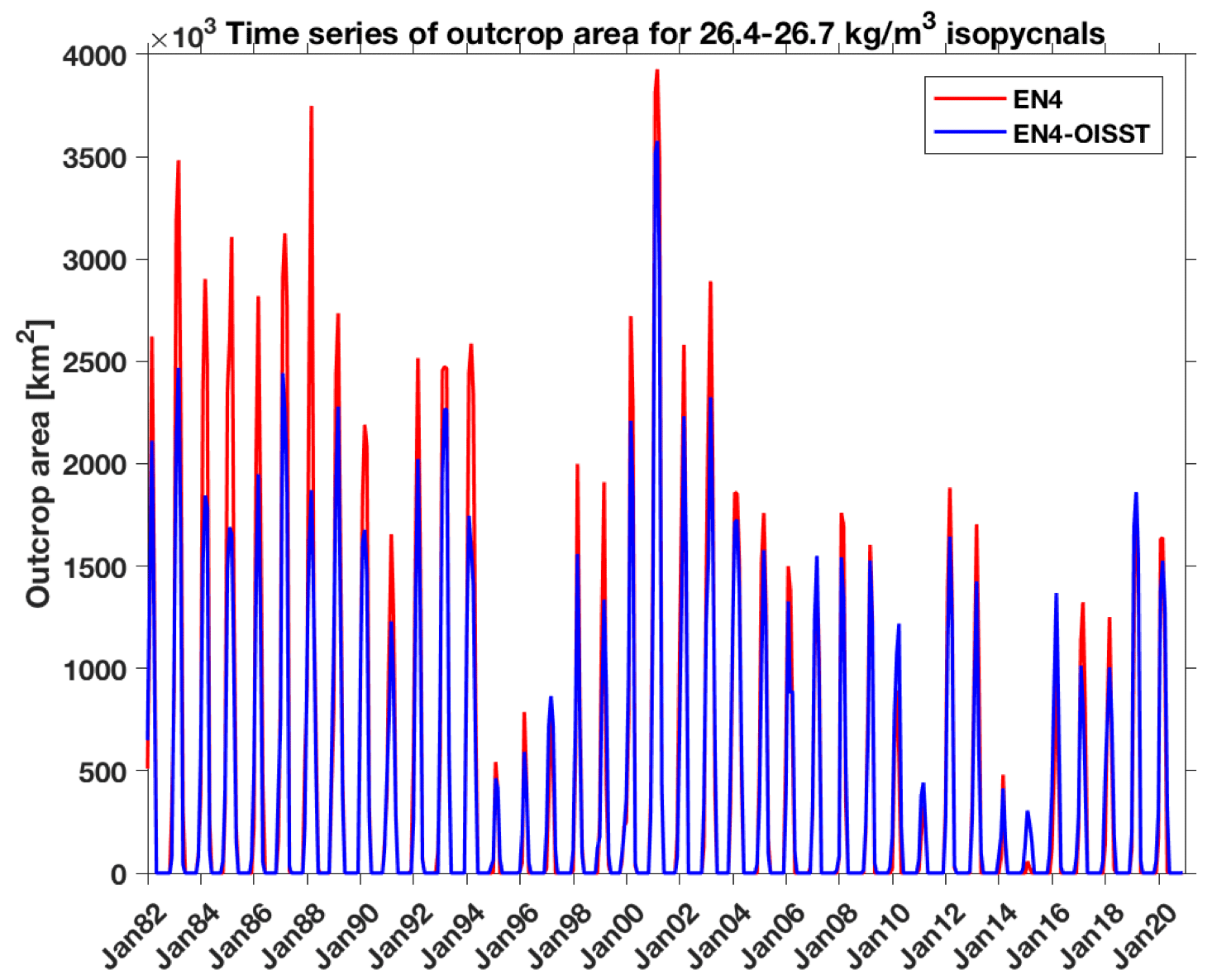
Figure 2Time series of the surface outcrop area of the σθ = 26.4–26.7 kg m−3 isopycnal range in the North Pacific from 1982–2020. The blue line is based on surface density from the ° EN4-OISST dataset, and the red line is based on surface density from the 1° EN4 dataset. The peaks in the outcrop area occur just after January (shown on the x axis) of each year, usually in March.
To assess how spatial resolution of data and small-scale variability affect the results, we compare EN4-OISST with the lower-resolution EN4 dataset (1° × 1°) that is based on EN4 temperature and salinity (Sect. 2.1). The time series of the σθ = 26.4–26.7 kg m−3 outcrop area from 1982 to 2020 using EN4 (Fig. 2; red line) exhibits larger March peak values than the EN4-OISST dataset (Fig. 2; blue line) does in almost every year, likely because SST fields in EN4 are more smoothed and less patchy than in the OISST satellite product. However, the EN4-derived outcrop areas show the same pattern of maxima and minima as EN4-OISST does, indicating that, in particular, the extreme minima in 1995–1997, 2011, and 2014–2015 and the extreme maximum in 2001 are robust results. The EN4-OISST and EN4 datasets (Fig. 2), despite the 2001 maximum, also both show a declining trend in the σθ = 26.4–26.7 kg m−3 outcrop area from 1982–2020, which is discussed further in the next section. We continue to use the EN4-OISST dataset for most of the remainder of the analysis given its higher resolution, knowing that the trends and overall patterns in outcrop area are consistent among the higher- and lower-resolution datasets.
In order to examine a longer time frame, we also calculate the σθ = 26.4–26.7 kg m−3 outcrop area for the full EN4 record since 1900 (Fig. A3) in addition to the 1982–2020 data shown in Fig. 2 (red line). Decadal variability in the outcrop area is also present prior to 1982 (Fig. A3), but the nearly constant outcrop area in the earlier part of the record (1900–1925) stands out as somewhat suspect. Since uncertainties reported with the EN4 data do not become larger going back in time to 1900, as one would expect for earlier data, measurement error/bias is likely not fully accounted for. Thus, in the following, we rely on the EN4-OISST dataset (as mentioned above), except when lag correlations are also calculated using the longer EN4 record (Sect. 3.2).
3.2 Correlations between outcrop area and O2 time series
Since OSP is downstream of the σθ = 26.4–26.7 kg m−3 outcrop area in the northwestern North Pacific (as indicated by streamlines on σθ = 26.6 kg m−3 in Fig. A2), O2 distributions observed at OSP, mapped onto a potential density anomaly versus time grid (Sect. 2.1), are expected to be affected by O2 uptake variability (i.e., ventilation variability) in the isopycnal outcrop region. For the OSP data, we confirm that there are large decadal variations in O2 concentration (Whitney et al., 2007; Cummins and Ross, 2020) on isopycnals near the bottom of the ventilated thermocline (Fig. 3a), where maximum O2 variability, based on repeat hydrography data, has been observed previously on the σθ = 26.6 kg m−3 isopycnal (Mecking et al., 2008). Figure 3b illustrates that densities around σθ = 26.6 kg m−3 are also the isopycnals where the largest decadal variations (and long-term O2 trends) occur at OSP, as indicated by overall maxima in standard deviation and in the negative trend of O2 over the time period of the OSP record (1956–2020) around σθ = 26.5–26.7 kg m−3. Maxima in declining O2 trends at OSP have also been reported in this density range by Whitney et al. (2007; σθ = 26.5 kg m−3) and Crawford and Peña (2016; σθ = 26.7 kg m−3), each using slightly different methodologies, but also slightly deeper on σθ = 26.8 kg m−3 (Cummins and Ross, 2020), which does not outcrop in the North Pacific, solidifying the fact that this is the density range of largest O2 decline or close to it in the northeastern North Pacific. Combining the O2 data on σθ = 26.6 kg m−3 with the time series of the annual maximum σθ = 26.4–26.7 kg m−3 outcrop area from the EN4-OISST dataset (maxima each year on the blue line in Fig. 2), which we use as a proxy for ventilation of the isopycnals at the bottom of the ventilated thermocline, shows that a strong minimum in O2 in 2005–2007 lags the minimum in annual maximum outcrop area in 1995–1997 by about a decade (Fig. 4; solid blue and cyan versus solid red and magenta lines, respectively). Such a lag is expected, assuming it takes about 10 years for surface waters from the outcrop area in the northwestern North Pacific to reach OSP on this isopycnal (Whitney et al., 2007). This transit time is somewhat larger than the 7–8-year west-to-east transit time estimated by Ueno and Yasuda (2003) on σθ = 26.7 kg m−3 from a North Pacific inverse model, but, given the differences in data and methods used and the notion that the O2 cycles in the northeastern North Pacific are affected by more than one process (Sasano et al., 2015, 2018), we consider our transit time estimate to be roughly consistent with Ueno and Yasuda's.
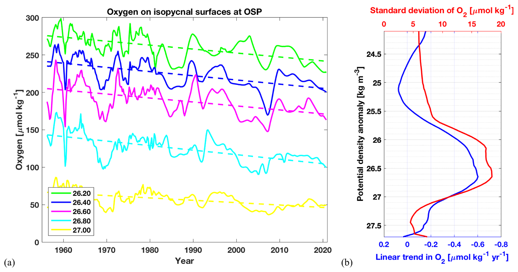
Figure 3(a) Time series of O2 at OSP (see location in Fig. 1) on isopycnals from σθ = 26.2–27.0 kg m−3 (in 0.2 kg m−3 increments). Linear trends of O2 on each isopycnal are shown as dashed lines. (b) Isopycnal profiles of the linear O2 trends (blue) and of the standard deviation of the O2 variations (red) on isopycnals (in 0.05 kg m−3 increments) at OSP. The vertical profiles were smoothed with a 9-point running average (corresponding to a 0.4 kg m−3 averaging interval). Data used are objectively mapped O2 data at OSP.
Estimation of lagged correlations between O2 on σθ=26.6 kg m−3 and the annual maximum σθ = 26.4–26.7 kg m−3 outcrop area from EN4-OISST, using the unfiltered time series (Fig. 4; solid blue and red lines, respectively) and the filtered data (Fig. 4; cyan and magenta lines, respectively), also results in the best correlation at a 10-year lag for the O2 record lagging the annual maximum outcrop area (r=0.50 for filtered detrended data where r is the linear correlation coefficient; Fig. 5). Note that the correlation is even better for O2 leading the annual maximum outcrop area (r=0.59 at a −10-year lag for O2; Fig. 5), which is unphysical, though, since O2 in the interior ocean does not have an obvious effect on surface density. However, since the O2 variations and possibly the annual maximum outcrop area are associated with bi-decadal cycles, shifting O2 either forward or backward in time by 10 years should result in a strong correlation with the outcrop area. This also explains why there is a maximum negative correlation at a close-to-zero lag (; Fig. 5).
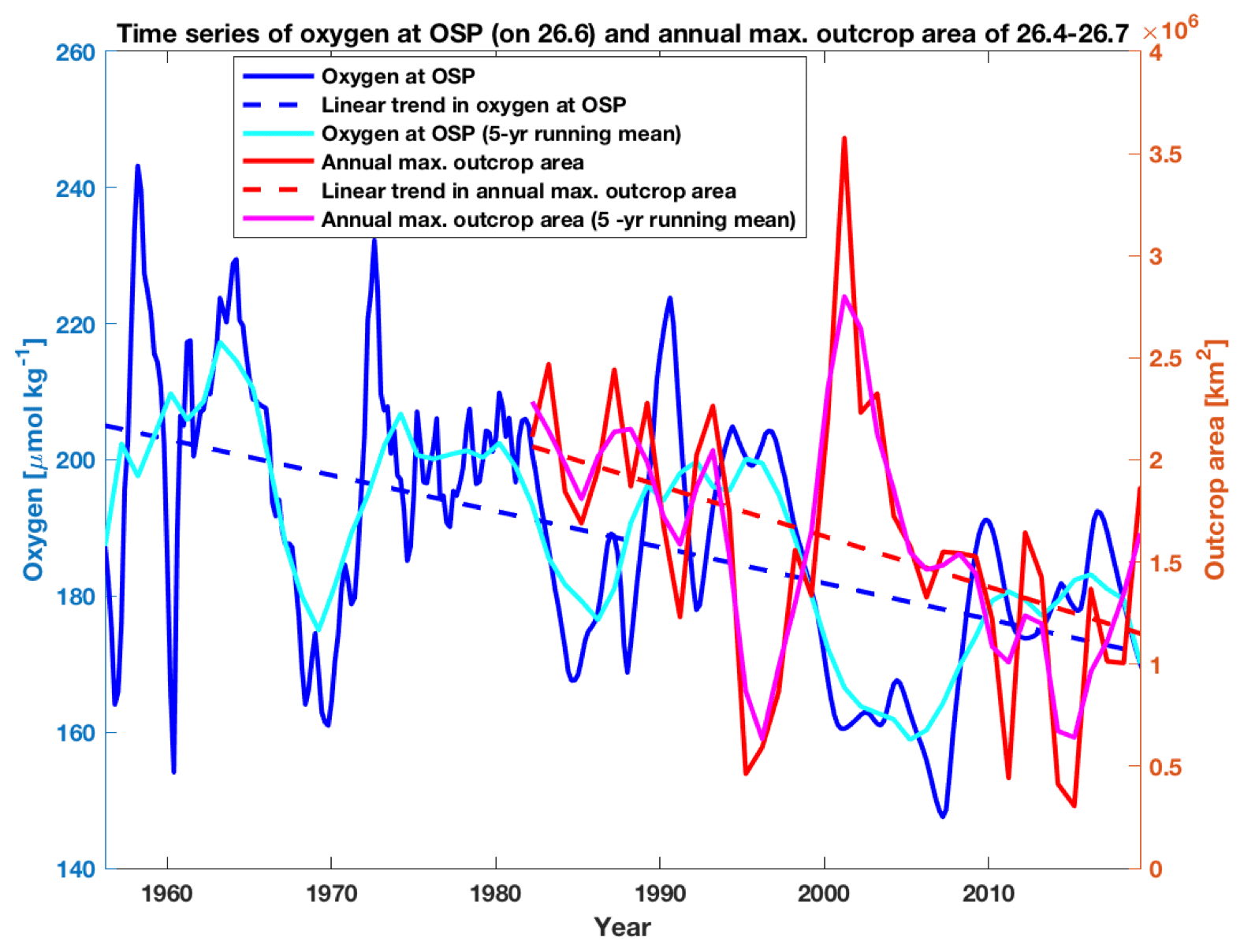
Figure 4Time series of O2 on σθ=26.6 kg m−3 at OSP (magenta line in Fig. 3a) and of annual maximum outcrop area of σθ = 26.4–26.7 kg m−3 based on the EN4-OISST dataset (blue line in Fig. 2) plotted on top of each other (solid blue and red lines, respectively). Also shown are the data filtered with a 5-year running mean (solid cyan and magenta lines, respectively) and the linear trends in each time series (dashed blue and red lines, respectively). The linear trends are −0.53 µmol kg−1 yr−1 for the O2 time series and m2 yr−1 for the outcrop area time series.
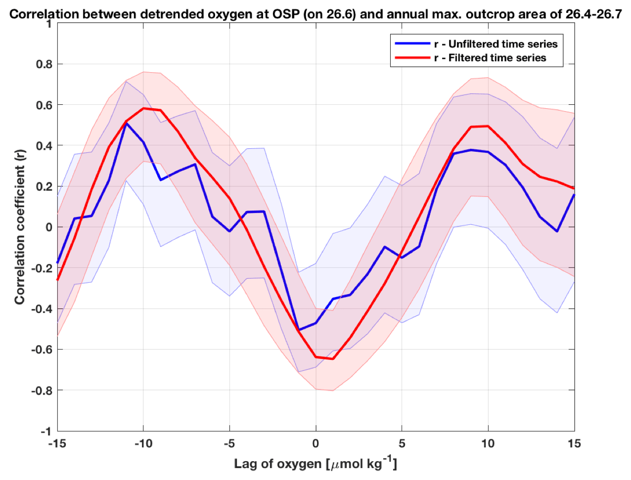
Figure 5Lagged correlations between detrended time series of O2 on σθ=26.6 kg m−3 at OSP and of annual maximum outcrop area of σθ = 26.4–26.7 kg m−3 from EN4-OISST (solid lines in Fig. 4 with linear trends, the dashed lines in Fig. 4, removed), using unfiltered time series data (blue line) and using the time series data filtered with a 5-year running mean (red line). The x axis represents the lag of the O2 time series relative to the outcrop area time series. Shaded areas show 95 % confidence intervals. Maximum correlation values (r) for the filtered data are 0.59 at a −10-year lag and 0.50 at a +10-year lag, and maximum negative r value (−0.65) occurs at close to a 0-year lag.
We note that on isopycnals deeper than σθ=26.6 kg m−3, the lag between O2 and the annual maximum σθ = 26.4–26.7 kg m−3 outcrop area tends to increase, as shown for σθ=27.0 kg m−3, where the best correlation for O2 lagging the outcrop area is at 14 years (Fig. A4) compared to 10 years for σθ=26.6 kg m−3 (Fig. 5). This finding is consistent with an increase in west-to-east travel times with density (and depth), as reported by Ueno and Yasuda (2003) using similar densities in their model calculations (see their Fig. 7). However, for isopycnals shallower than σθ=26.6 kg m−3, we do not find a depth trend in the lag between O2 and outcrop area (not shown) because the O2 cycles at OSP on isopycnals between σθ=26.2 kg m−3 and σθ=26.6 kg m−3 are in phase (Fig. 3a). We hypothesize that the O2 signal that peaks near σθ=26.6 kg m−3 (Fig. 3b) is distributed to the lighter (i.e., shallower) isopycnals through vertical mixing as the water travels west to east, and the O2 signals at σθ=26.6 kg m−3 and above are thus in sync with each other. In contrast, for the isopycnals below σθ=26.6 kg m−3, which correspond to the upper North Pacific Intermediate Water (NPIW) range (σθ = 26.64–27.0 kg m−3; Talley, 1997), the O2 signals may be dominated by the vertical mixing processes in the northwestern North Pacific that are part of the formation process of NPIW (Sasano et al., 2018). NPIW travels eastward then at a slower rate than water on σθ=26.6 kg m−3 (Ueno and Yasuda, 2003), causing the O2 signals to be out of phase with the shallower layers.
In order to examine a longer time frame, we also calculate lagged correlations between O2 on σθ=26.6 kg m−3 at OSP and the σθ = 26.4–26.7 kg m−3 outcrop area based on the entire EN4 record (Fig. A3) using data since 1941 (Fig. A5; since the O2 record at OSP starts in 1956, 1941 is the first data year used for outcrop area when calculating correlations with a maximum lag of 15 years) instead of the EN4-OISST dataset (Fig. 5). Maximum correlations using EN4 also occur at close to ±10-year lags (Fig. A5). The magnitude of the maximum correlations is smaller than for the EN4-OISST dataset (Fig. 5), which may be a result of the lower accuracy of the earlier data in EN4. Nevertheless, the maximum correlations are statistically significant, and the conclusion remains consistent that O2 on σθ=26.6 kg m−3 at OSP lags variations in outcrop area by about 10 years.
In addition to decadal-scale variability, both the OSP O2 time series on σθ=26.6 kg m−3 and the northwestern North Pacific annual maximum outcrop area (Fig. 4) exhibit declining long-term linear trends amounting to −0.53 µmol kg−1 yr−1 and m2 yr−1, respectively (dashed lines in Fig. 4). Previous studies have shown that there is a long-term decrease in O2 at OSP (Whitney et al., 2007; Stramma et al., 2020) and in surface density in the northwestern North Pacific (Ono et al., 2001; Durack and Wijffels, 2010), the latter of which is consistent with the decreasing trend in the outcrop area of the densest outcropping isopycnals (σθ = 26.4–26.7 kg m−3) that we have shown here. The trends in O2 and outcrop area likely occur together for the same reasons that the decadal-scale variability in O2 at OSP and outcrop area are correlated (with O2 lagging; see above): as the outcrop area of the σθ = 26.4–26.7 kg m−3 isopycnals declines, less ventilation of these isopycnals takes place, and less O2 is transported from the mixed layer into the ocean interior, causing the declining trend in O2 on those isopycnals at OSP.
One caveat to the interpretation of the OSP O2 data in combination with the northwestern North Pacific outcrop area time series comes from repeat hydrography data in the area of OSP (Fig. A2). Near the latitude and longitude of OSP (50° N, 145° W), CLIVAR/GO-SHIP repeat hydrography section differences show continued O2 decline from the mid-2000s to the mid-2010s along 152° W (P16N; 2015 minus 2006; Fig. A6a) and along 47° N (P1; 2014 minus 2007; Fig. A6b; see also Kouketsu et al., 2020, their Fig. 4b). This is contrary to the OSP data, which indicate an increase in O2 on the σθ=26.4 kg m−3 to σθ=27.0 kg m−3 isopycnals between those points in time (Fig. 3a). To resolve this, we combine O2 values from the CLIVAR/GO-SHIP and earlier WOCE sections, averaged zonally on isopycnals over the intervals 40–45° N for P16N and 140–165° W for P1 (intervals shown as black lines in Fig. A6), with the OSP time series directly (Fig. A7). This indicates that (1) the section averages for both P16N (Fig. A7a) and P1 (Fig. A7b) may lead the OSP time series by 2–4 years, suggesting that O2 signals arrived at the hydrographic section locations a few years earlier than at OSP and that they follow perhaps a longer, more eastward pathway from 47° N to OSP than the climatological streamlines in Fig. A2 indicate (Kouketsu et al., 2020), and that (2) the repeat hydrography, due to lack of time resolution, does not fully resolve the temporal variability in the O2 record and misses, for example, the large O2 minimum observed at OSP in 2007 that leads the 2010s increase in O2. While the 2–4-year lead of the section data is larger than one might expect given the proximity of the sections to OSP, we conclude that the repeat hydrography data (within the limits of decadal observations) are still roughly consistent with the OSP data in terms of observed O2 changes.
3.3 Causes
3.3.1 SSS and SST variability
As outlined in the previous section (Sect. 3.2), variability in oxygen at OSP in the eastern North Pacific can be explained in part by upstream fluctuations in isopycnal outcrop areas in the northwestern North Pacific with a lag of about 10 years (Figs. 4, 5). Here, we assess the drivers of the outcrop area fluctuations by examining the effects of SST and SSS in the northwestern North Pacific (averaged over 40–50° N, 150–170° E; see box in Fig. 1a) on surface density (Fig. 6). Contributions of SST and SSS (Fig. 6a) to annual maximum surface density changes in this area (Fig. 6b) are estimated by determining the annual mean cycle of SST and SSS each from the EN4-OISST dataset (also averaged over 40–50° N, 150–170° E) and then calculating surface density with either SST or SSS fixed (at its annual mean cycle) while allowing the other variable to vary (thin solid lines in Fig. 6a).
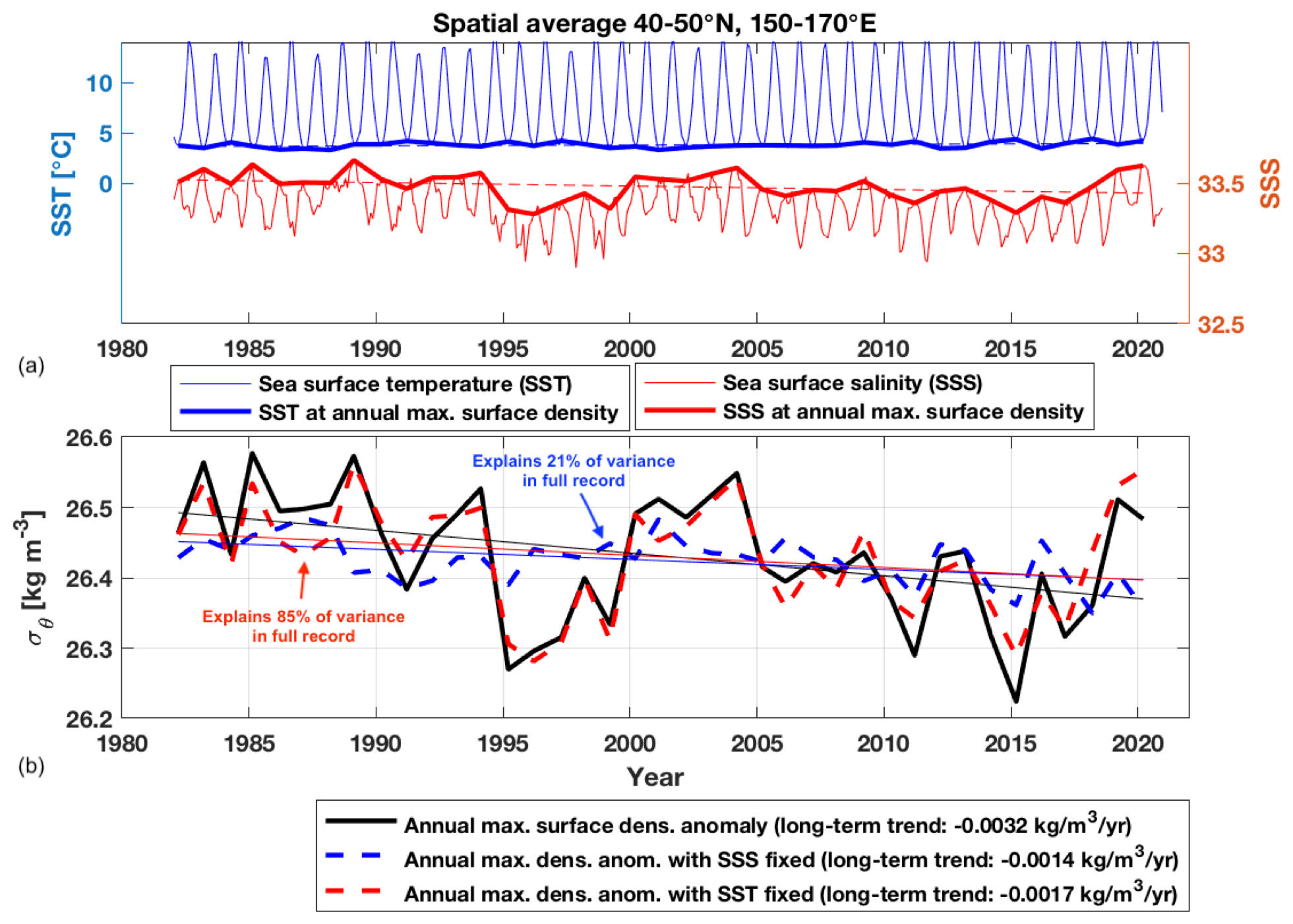
Figure 6(a) SST (bold blue line) and SSS (bold red line) at annual maximum surface density and (b) annual maximum surface density anomaly (bold black line) and contributions from SST (dashed blue line; with SSS fixed at mean annual cycle during density calculation) and SSS (dashed red line; with SST fixed at mean annual during density calculation) in the northwestern North Pacific (averaged over 40–50° N, 150–170° E; see Fig. 1a for area). The dashed red line (SST fixed) and dashed blue line (SSS fixed) in (b) explain 85 % and 21 % of variance of the full record (bold black line), respectively. Linear trends (dashed lines in a and thin solid lines in b, using respective colors) are also shown. Thin solid lines in (a) represent monthly SST and SSS values. Dataset used is the EN4-OISST dataset.
The SSS data at the time of annual maximum surface density (Fig. 6a; bold red line), usually late winter, show minima around 1996, 2011, and 2015. These match the years when the annual maximum σθ = 26.4–26.7 kg m−3 outcrop area has minima (Fig. 2) and the annual maximum surface densities are the lowest (Fig. 6b; bold black line). Varying SSS and keeping SST fixed at its annual mean cycle result in annual maximum surface densities (Fig. 6b; dashed red line) that follow the annual maximum surface density (bold black line) closely, which indicates that variations in SSS are the main driver of interannual variations in annual maximum surface density in the northwestern North Pacific. This includes a rebound to higher surface densities in recent years that is evident in both the total and the SSS-driven density records (Fig. 6b) and that is caused by the increase in SSS since 2017 (Fig. 6a). In contrast, varying SST and keeping SSS fixed at its annual mean cycle cause much smaller interannual variations in the annual maximum surface density (Fig. 6b; dashed blue line) than observed in the full record (bold black line), confirming the lesser role that SST plays in producing the interannual annual maximum surface density variations in the northwestern North Pacific.
Quantitatively, SSS-driven (SST fixed) and SST-driven (SSS fixed) density variability can explain 85 % and 21 %, respectively, of the variance in total annual maximum surface density in Fig. 6b. The contributions do not add up to 100 % exactly, due to the non-linearities in the calculation of density (equation of state), but it is clear that SSS variations have a much larger contribution (about 4 times). The dominance of salinity over temperature in driving density fluctuations is consistent with the relatively large haline contraction coefficient compared to the thermal expansion coefficient at this latitude, which govern the contributions of salinity and temperature, respectively, to density (McDougall and Barker, 2011). In terms of long-term linear density trends (Fig. 6b; thin solid lines), the SSS-based trend (thin red line; −0.0014 kg m−3 yr−1) and the SST-based trend (thin blue line; −0.0017 kg m−3 yr−1) contribute about equally to the linear decrease in total annual maximum surface density (thin black line; −0.0032 kg m−3 yr−1), indicating that long-term surface freshening and warming in the northwestern North Pacific are of similar importance in explaining declining surface densities.
Evidence that SSS variations in the northwestern North Pacific are occurring and playing a major role in determining interannual changes in upper-ocean density and related ventilation also comes from a study by Uehara et al. (2014), who found upper-layer (0–100 m) salinity variability in the Western Subarctic Gyre (WSG; their Fig. 4) similar to the SSS variability reported here (Fig. 6a), with our averaging area (see box in Fig. 1a) encompassing the southern half of their WSG definition. The time period examined in Uehara et al. (2014) is 1950 to 2008, overlapping the time period of our surface time series (1982–2020) by 26 years and showing the strongest surface salinity freshening signals in the WSG in the early 1960s and in the late 1990s, with the latter corresponding to the SSS minimum we find around 1996 (Fig. 6a) and the strong reduction in the March outcrop area of σθ = 26.4–26.7 kg m−3 from 1995–1997 (Fig. 2). Uehara et al. (2014) attribute the upper-ocean salinity changes in the WSG to changes in atmospheric forcing, such as precipitation and wind, and suggest that these changes are propagated downstream by surface currents into the Bering Sea, the eastern Kamchatka region, the eastern Sea of Okhotsk, and finally the shelves in the northwestern Sea of Okhotsk (see pathways in their Fig. 9), where dense shelf waters are formed due to surface cooling. Along this path, mixing variability associated with the 18.6-year nodal tidal cycle, which has been quoted by several authors as a source of upper-ocean variability in the northwestern North Pacific, especially around the narrow passages in the Kuril Straits that separate the Sea of Okhotsk from the northwestern North Pacific (Yasuda et al., 2006; Whitney et al., 2007; Osafune and Yasuda, 2013; Stramma et al., 2020), may affect upper-layer salinities (Uehara et al., 2014). Based on the findings by Uehara et al. (2014) that the WSG is at the upstream end of this surface water pathway, however, we conclude that the SSS and outcrop area variability in the northwestern North Pacific reported here (as well as the associated ocean interior O2 changes at OSP in the northeast) are also due to atmospheric forcing changes rather than the nodal tidal cycle, as has been speculated (Whitney et al.., 2007). Nevertheless, there could be feedback loops from the dense shelf waters produced in the Sea of Okhotsk at the downstream end of this path back to the surface waters in the open northwestern North Pacific.
3.3.2 Climate indices (PDO, NPGO, and NPI)
The PDO is the dominant mode of variability in the North Pacific Ocean, with the PDO index defined as the leading principal component of monthly SST variability north of 20° N (Mantua et al., 1997). Since much of the variability in annual maximum surface density that we associate with fluctuations in the σθ = 26.4–26.7 kg m−3 outcrop area and O2 downstream appears to be driven by salinity variations, as illustrated in the previous section (Sect. 3.3.1), a correlation between surface density and the PDO is not necessarily expected. Indeed, we find that the correlation between the PDO and the annual maximum surface density (averaged over 40–50° N, 150–170° E) time series (Fig. A8) has an r value of only 0.03. There are periods where the two time series seem to be tracking each other (1999–2005) but also several where they clearly show opposite variations (e.g., 1995–1999, 2013–2018), resulting in a correlation close to 0.
Only somewhat higher correlations exist between the annual maximum surface density and the North Pacific Gyre Oscillation (NPGO) index (Di Lorenzo et al., 2008) and between annual maximum surface density and the North Pacific Index (NPI; Trenberth and Hurrell, 1994) with r values of 0.16 (Fig. A9) and −0.14 (Fig. A10), respectively, suggesting that these indices also describe little of the surface density variability that drives downstream O2 variations at OSP. The NPGO index is defined as the second mode of sea surface height (SSH) anomaly variability in the northeastern North Pacific (Di Lorenzo et al., 2008), whereas the NPI represents area-weighted wintertime sea level pressure over the northern North Pacific (30–65° N, 160° E–140° W), which indicates changes in atmospheric circulation. Note that correlations between climate indices and North Pacific thermocline O2 changes have also been analyzed in different ways (Andreev and Kusakabe, 2001; Ono et al., 2001; Mecking et al., 2008; Stramma et al, 2020), with connections between OSP O2 and the PDO (Mecking et al., 2008; Stramma et al., 2020), as well as the NPGO (Stramma et al., 2020), found to be weak or inconclusive, but that we focus here on the correlations of climate indices with northwestern North Pacific surface density changes because we are evaluating surface density changes as a driving force for OSP O2 changes in this paper. However, given the dominance of SSS in driving annual maximum surface density changes and the relatively low correlations between the surface density changes and the PDO, NPI, or NPGO, we conclude that a climate index that better incorporates salinity is needed, for example, through inclusion of SSS and/or E−P (evaporation minus precipitation) data, since E−P variability is the main driver for SSS changes (Durack and Wijffels, 2010).
Analysis of annual maximum outcrop areas of the densest isopycnals to reach the surface in the northwestern North Pacific in winter indicates that there are significant interannual variations, as shown by the time series of the σθ = 26.4–26.7 kg m−3 outcrop area in the EN4-OISST dataset starting in 1982 (Fig. 2). We consider the size of these outcrop areas as an indicator of how much ventilation is occurring at the bottom of the ventilated thermocline in the North Pacific, since renewal of interior waters from the mixed layer and uptake of gases only occur when isopycnals outcrop. A significant 10-year lagged correlation exists between the σθ = 26.4–26.7 kg m−3 outcrop area variations and the ∼ bi-decadal O2 cycles at OSP in the northeastern North Pacific that exhibit the largest variability within this density range, giving support to the hypothesis that surface density variations are a main driver of O2 changes in the ocean interior. This is consistent with the findings by Sasano et al. (2018) that ventilation variability is a key process in generating O2 trends and oscillations on isopycnals that outcrop in the North Pacific (σθ < 26.8 kg m−3; see their Fig. 11). The 10-year lag corresponds approximately to the travel time of newly ventilated (and oxygenated) waters from the isopycnal outcrop locations in the northwestern North Pacific to OSP in the northeast, where the isopycnals have descended to the subsurface. Kwon et al. (2016) found similar connections between isopycnal outcropping and ocean interior O2 changes using a data-assimilating ocean circulation model, whereas the results here are entirely data-based.
A new finding in our analysis is the dominance of SSS over SST in driving interannual fluctuations in annual maximum surface density (a ventilation proxy similar to annual maximum σθ = 26.4–26.7 kg m−3 outcrop area) in the northwestern North Pacific, as shown in Fig. 6b. Evidence that SSS variations in the northwestern North Pacific are occurring and play a major role in determining interannual changes in upper-ocean density and the related ventilation also comes from the analysis of SSS of shelf waters in the adjacent Sea of Okhotsk (Uehara et al., 2014). In contrast, SSS (freshening) and SST (warming) contribute about equally to the long-term declining density trends in the northwestern North Pacific (Fig. 6b) that are the cause of the long-term linear decline in the σθ = 26.4–26.7 kg m−3 outcrop area and subsequently O2 concentrations at OSP (Fig. 4) as well.
In contrast to Kwon et al. (2016), we do not find a good correlation between annual maximum surface density (or outcrop area) and thus ventilation and the PDO or other climate indices (NPGO, NPI). This may be because the analysis in this paper is using independent datasets and not a model, where forcing and ocean response are consistent by design. However, given the dominance of SSS in determining interannual variations in surface density, a correlation with the PDO (which is based on SST) is not necessarily expected. While it is beyond the scope of this paper, we suggest for future work the development of a North Pacific climate index that captures the SSS variability in the northwestern North Pacific and the expansion of this work to include data-based subduction rates.
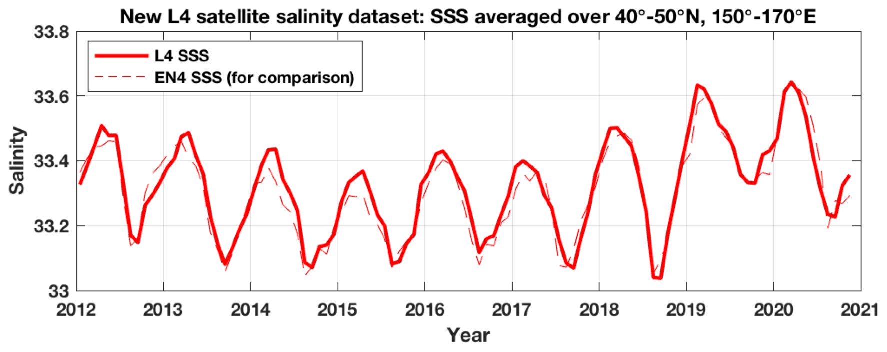
Figure A1Satellite sea surface salinity (SSS) in the northwestern North Pacific averaged over 40–50° N, 150–170° E (see Fig. 1a for area) using the new Multi-Mission Optimally Interpolated Sea Surface Salinity (OISSS) Level-4 V1.0 dataset (Melnichenko et al., 2016). Also shown are SSS averages from the EN4 dataset (dashed line) for comparison.
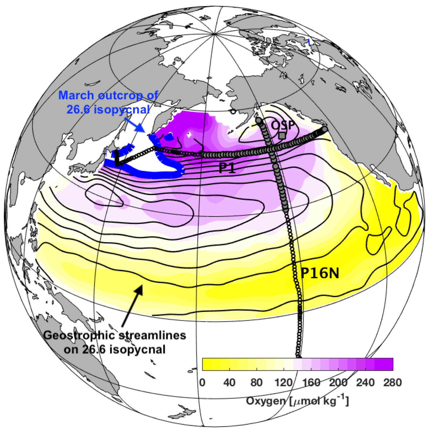
Figure A2Dissolved oxygen (color shading) on σθ=26.6 kg m−3 in the North Pacific. Black contours mark streamlines (acceleration potential; Huang and Qiu, 1994) on the σθ=26.6 kg m−3 isopycnal, and the bold blue contour marks the outcrop of this isopycnal in late winter (March). Oxygen decreases following streamlines because of respiration in the ocean interior. Data are from the World Ocean Atlas (Levitus and US National Oceanographic Data Center, 2012) and represent the climatological mean over several decades, similar to Fig. 1 in Mecking et al. (2008), but using oxygen instead of apparent oxygen utilization data. In addition, circles mark station locations of the CLIVAR/GO-SHIP repeat hydrography cruises P16N and P1, with the larger gray-faced circles indicating the latitude and longitude ranges, respectively, of stations used for the difference plots in Fig. A6. The location of Ocean Station P (OSP; Whitney et al., 2007) is marked by a gray square.
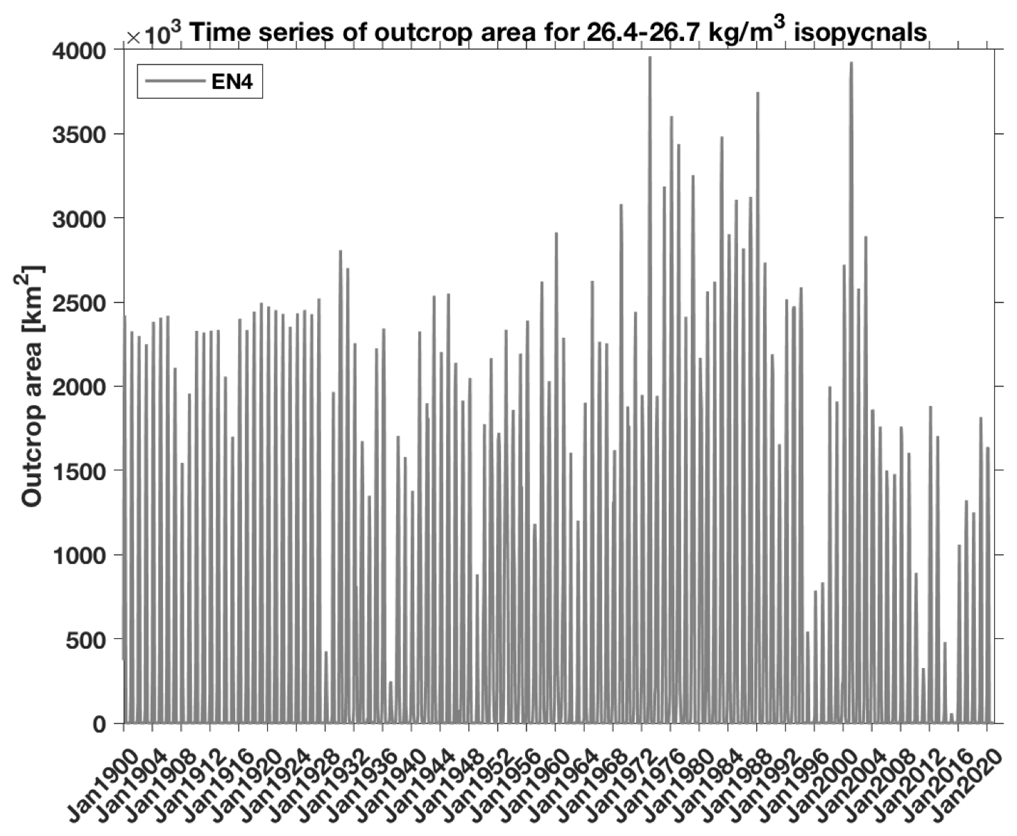
Figure A3Time series of surface outcrop area of the σθ = 26.4–26.7 kg m−3 isopycnal range in the North Pacific, from the 1° EN4 dataset, for the full 1900–2020 record. The data since 1982 are the same as shown for EN4 in Fig. 2 (red line).
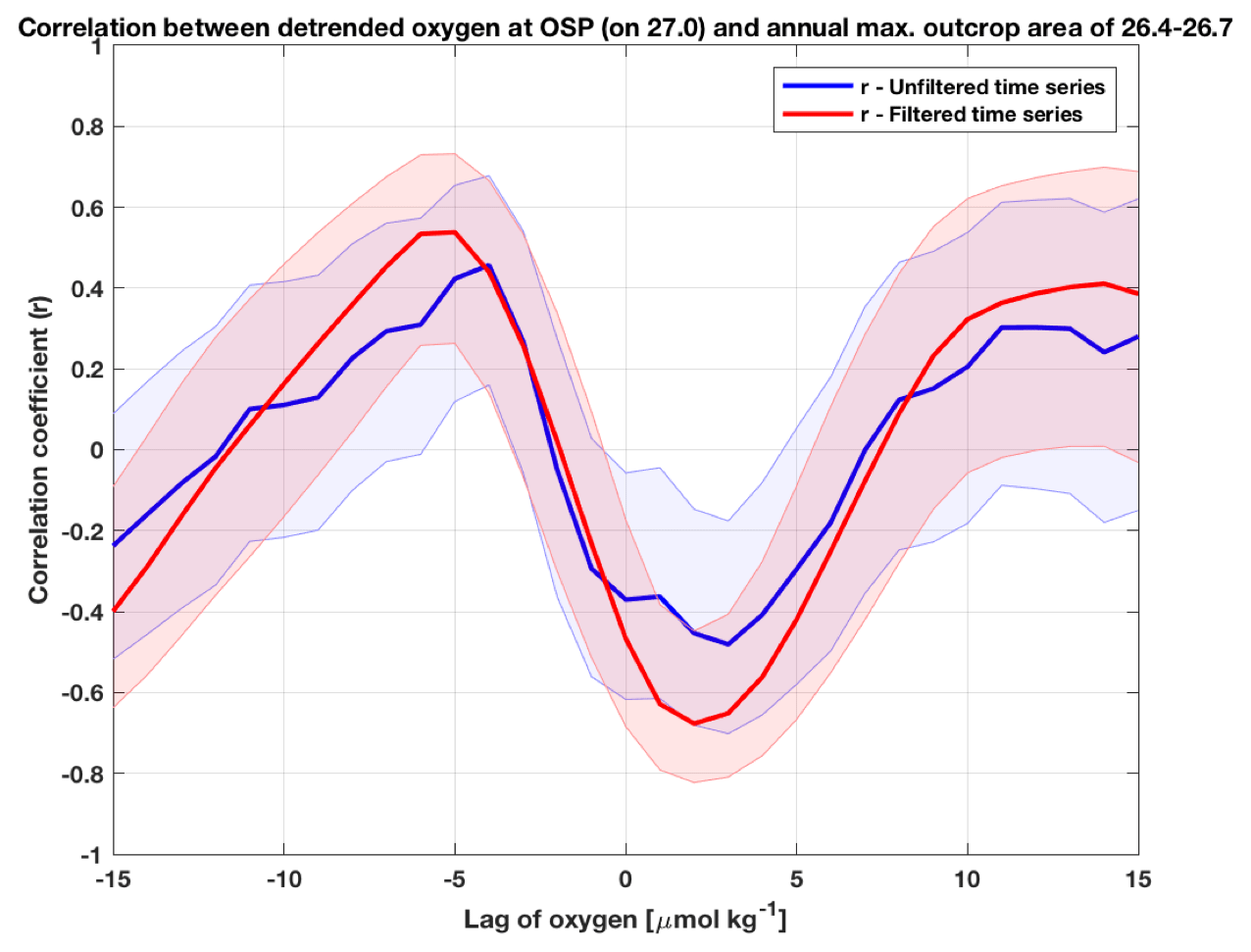
Figure A4Lagged correlations between detrended time series of O2 on σθ=27.0 kg m−3 at OSP (solid yellow line in Fig. 3a) and of annual maximum outcrop area of σθ = 26.4–26.7 kg m−3 from EN4-OISST (red/magenta lines in Fig. 4), using unfiltered time series data (blue line) and time series data filtered with a 5-year running mean (red line). Details follow Fig. 5.
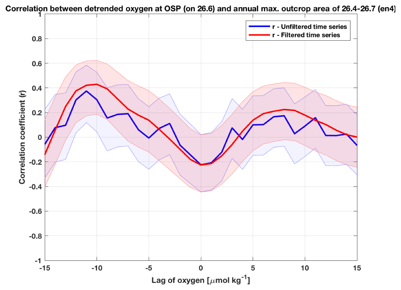
Figure A5Lagged correlations between detrended time series of O2 on σθ=26.6 kg m−3 at OSP (1956–2020; blue/cyan lines in Fig. 4) and of annual maximum outcrop area of σθ = 26.4–26.7 kg m−3 from EN4 (using the 1941–2020 portion of the full outcrop area time series shown in Fig. A3), using unfiltered time series data (blue line) and time series data filtered with a 5-year running mean (red line). Details follow Fig. 5.
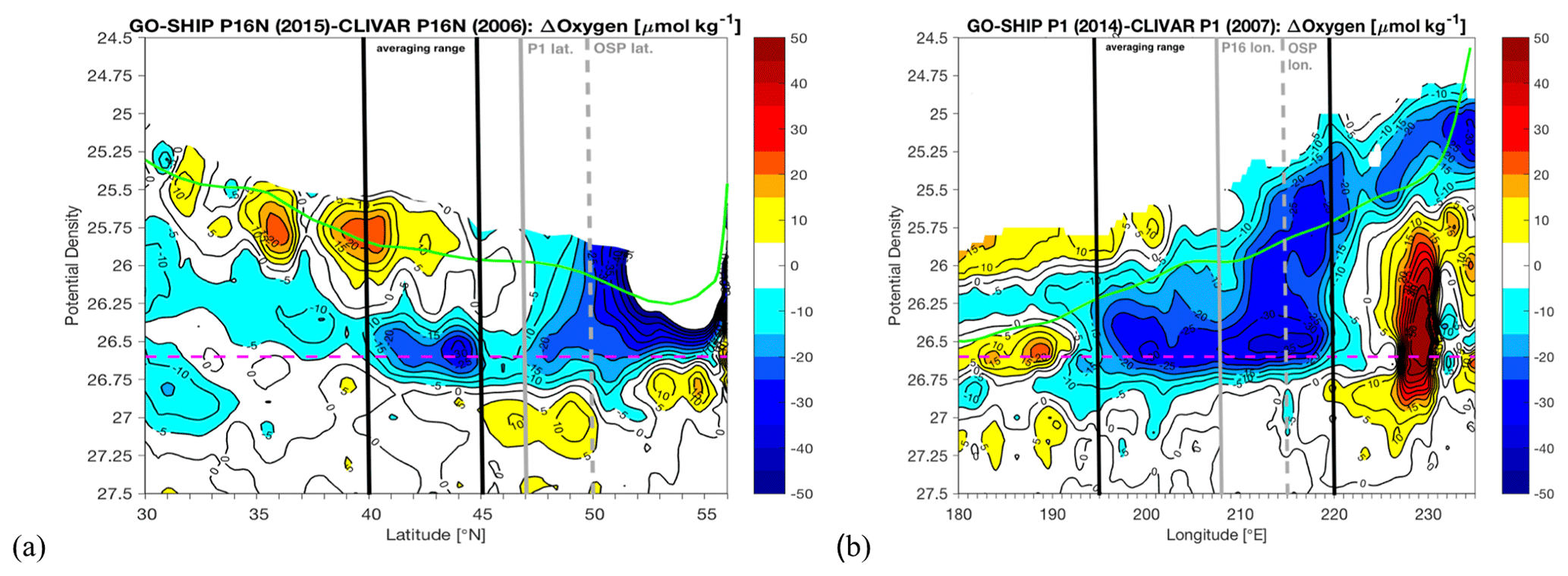
Figure A6O2 differences on potential density surfaces (color shading and thin black contour lines) for portions of two North Pacific repeat hydrography sections collected as part of CLIVAR/GO-SHIP: (a) along 152° W (P16N; 2015 minus 2006) and (b) along 47° N (P1; 2014 minus 2007). The locations of the sections relative to OSP are shown in Fig. A2. Changes are calculated by objectively mapping the O2 data from each repeat occupation to create latitude/longitude versus density grids and differencing the mapped data. The dashed magenta line in each panel marks the σθ=26.6 kg m−3 isopycnal. The light-green lines mark the March mixed-layer density along the sections, calculated from climatological data. The latitude and longitude of OSP are marked in (a) and (b), respectively, as dashed gray lines, and the latitude and longitude where P16N and P1 cross are marked in (a) and (b), respectively, as solid gray lines. The two bold black lines in each panel mark the averaging intervals used for Fig. A7. Note that the averaging interval (40–45° N) in (a) is somewhat to the south of the OSP latitude because this marks the region of largest O2 decline on σθ=26.6 kg m−3 in the interior away from the mixed layer and matches the averaging interval used in previous work (Mecking et al., 2008).
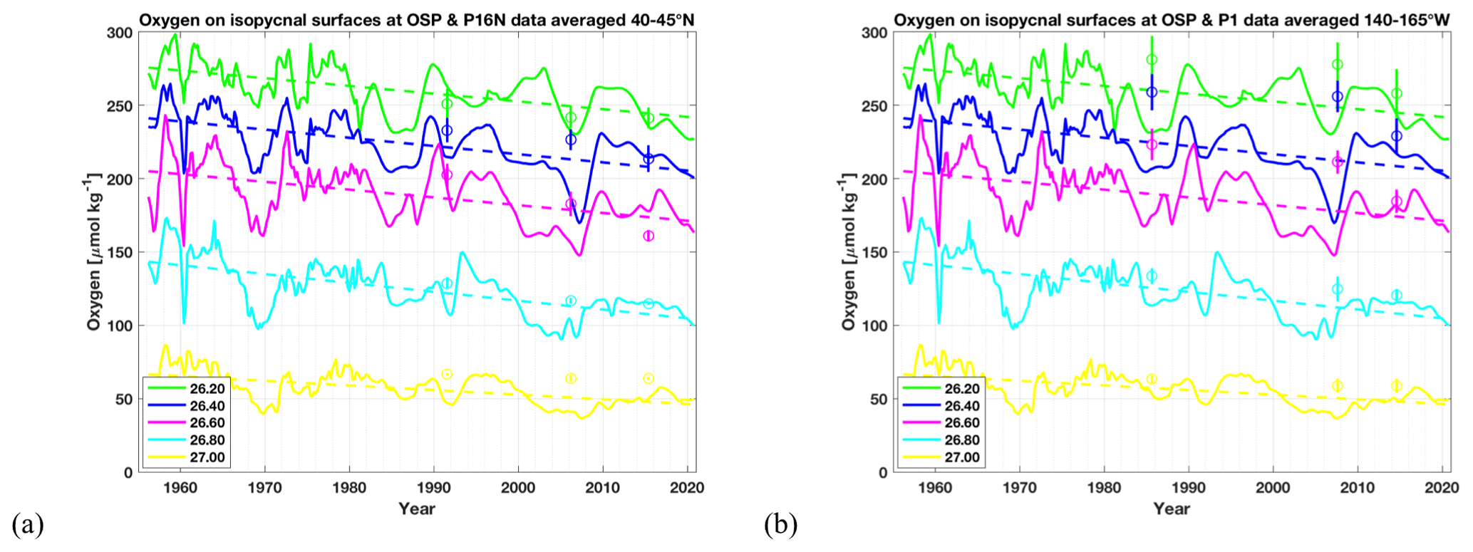
Figure A7O2 at OSP on isopycnals from σθ = 26.2–27.0 kg m−3 (in 0.2 increments), including linear trends (dashed lines), as in Fig. 3a, together with averages on the same isopycnals from the WOCE (late 1980s/early 1990s), CLIVAR (2000s), and GO-SHIP (2010s) repeat hydrography cruises, indicated by circles (mean) and vertical lines (standard deviation). Panel (a) uses averages between 40–45° N for P16N cruises along 152° W in 1991, 2006, and 2015, and panel (b) uses averages between 140–165° W for P1 cruises in 1985, 2007, and 2014. The latitudinal (P16N) and longitudinal (P1) averaging intervals are shown by the bold black lines in Fig. A6a and b, respectively.
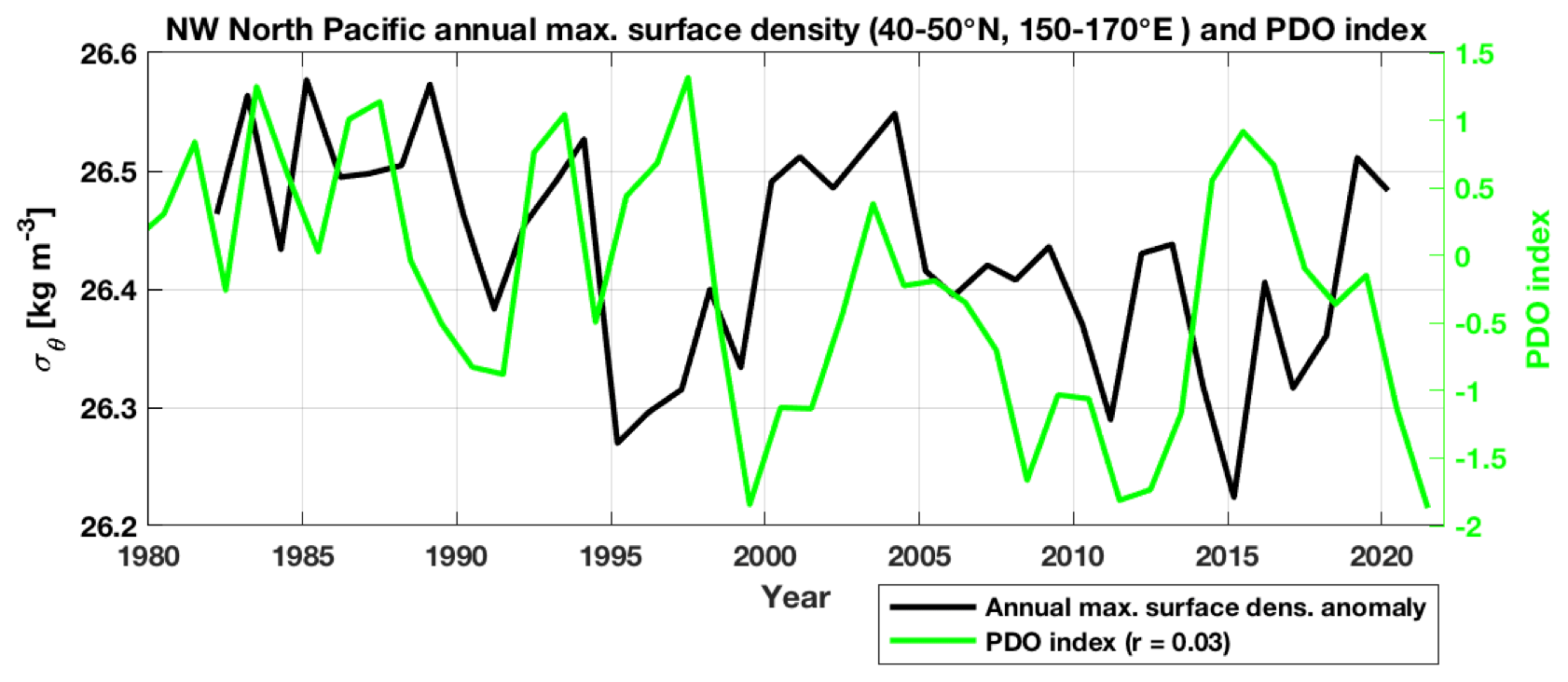
Figure A8Annual maximum surface density anomaly in the northwestern North Pacific averaged over 40–50° N, 150–170° E (black; same as the bold black line in Fig. 6b) and annually averaged Pacific Decadal Oscillation (PDO; Mantua et al., 1997) index (light green).
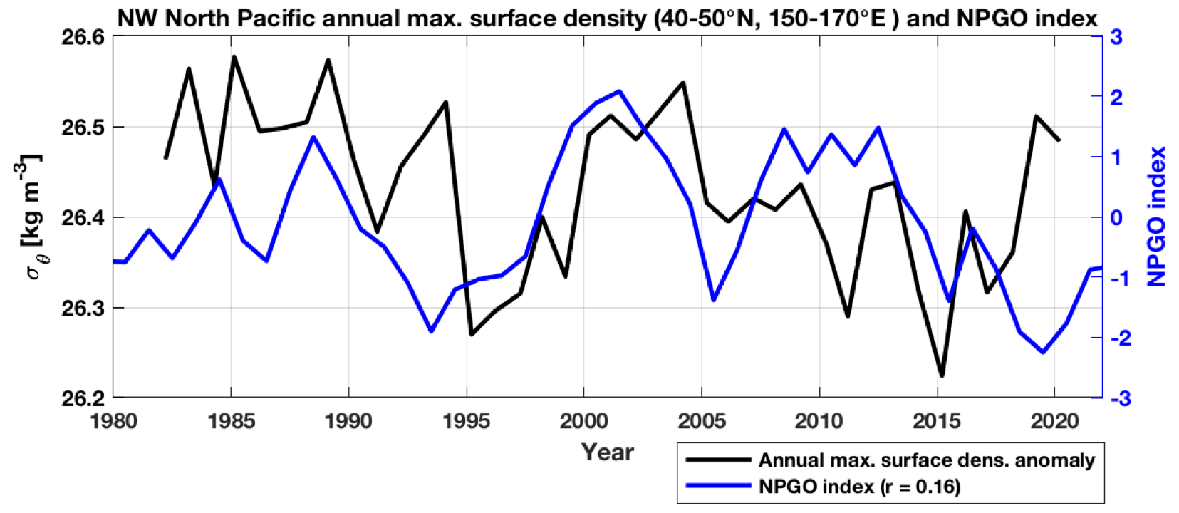
Figure A9Annual maximum surface density anomaly in the northwestern North Pacific averaged over 40–50° N, 150–170° E (black; same as the bold black line in Fig. 6b) and annually averaged North Pacific Gyre Oscillation (NPGO; Di Lorenzo et al., 2008) index (blue).
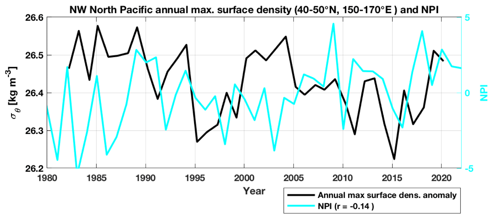
Figure A10Annual maximum surface density anomaly in the northwestern North Pacific averaged over 40–50° N, 150–170° E (black; same as the bold black line in Fig. 6b) and annually averaged North Pacific Index (NPI; Trenberth and Hurrell, 1994) in cyan.
The data used in this paper are available at the following websites:
-
EN4 – https://www.metoffice.gov.uk/hadobs/en4 (Good et al., 2013)
-
OISST – https://psl.noaa.gov/data/gridded/data.noaa.oisst.v2.highres.html (Reynolds et al., 2007)
-
OISSS – https://doi.org/10.5067/SMP10-4U7CS (Melnichenko, 2021)
-
OSP – https://www.waterproperties.ca/linep (Whitney et al., 2007)
-
WOCE/CLIVAR/GO-SHIP data – https://cchdo.ucsd.edu (Talley et al., 2016)
-
PDO – https://www.ncei.noaa.gov/pub/data/cmb/ersst/v5/index/ersst.v5.pdo.dat (Mantua et al., 1997)
-
NPI – https://climatedataguide.ucar.edu/climate-data/north-pacific-np-index-trenberth-and-hurrell-monthly-and-winter (Hurrell et al., 2023)
-
NPGO – http://www.o3d.org/npgo/ (Di Lorenzo et al., 2008)
-
World Ocean Atlas climatology – https://www.ncei.noaa.gov/archive/accession/0095184 (Levitus and US National Oceanographic Data Center, 2012)
SM and KD designed the study and wrote the article. SM was the project lead and made all the figures in the article. KD was the lead on analyzing the satellite data and combining them with other data products.
The contact author has declared that neither of the authors has any competing interests.
Publisher’s note: Copernicus Publications remains neutral with regard to jurisdictional claims made in the text, published maps, institutional affiliations, or any other geographical representation in this paper. While Copernicus Publications makes every effort to include appropriate place names, the final responsibility lies with the authors.
This article is part of the special issue “Low-oxygen environments and deoxygenation in open and coastal marine waters”. It is a result of the 53rd International Colloquium on Ocean Dynamics (3rd GO2NE Oxygen Conference), Liège, Belgium, 16–20 May 2022.
We would like to thank Roberta Hamme for input on a draft version of this paper, Tetjana Ross and the two anonymous reviewers for their comments on the submitted article, and Fisheries and Oceans Canada for making the OSP data publicly available. We are grateful to the National Science Foundation for financial support of this work.
This research has been supported by the U.S. National Science Foundation, Directorate for Geosciences (grant no. OCE-1851149).
This paper was edited by Carolin Löscher and reviewed by Tetjana Ross and two anonymous referees.
Anderson, L. A. and Sarmiento, J. L.: Redfield ratios of remineralization determined by nutrient data analysis, Global Biogeochem. Cy., 8, 65–80, https://doi.org/10.1029/93GB03318, 1994.
Andreev, A. G. and Baturina, V. I.: Impacts of tides and atmospheric forcing variability on dissolved oxygen in the subarctic North Pacific, J. Geophys. Res., 111, C07S10, https://doi.org/10.1029/2005JC003103, 2006.
Andreev, A. G. and Kusakabe, M.: Interdecadal variability in dissolved oxygen in the intermediate water layer of the Western Subarctic Gyre and Kuril Basin (Okhotsk Sea), Geophys. Res. Lett., 28, 2453–2456, https://doi.org/10.1029/2000GL012688, 2001.
Banzon, V., Smith, T. M., Chin, T. M., Liu, C., and Hankins, W.: A long-term record of blended satellite and in situ sea-surface temperature for climate monitoring, modeling and environmental studies, Earth Syst. Sci. Data, 8, 165–176, https://doi.org/10.5194/essd-8-165-2016, 2016.
Bretherton, F. P., Davis, R. E., and Fandry, C. B.: A technique for objective analysis and design of oceanographic experiments applied to MODE-73, Deep-Sea Res., 23, 559–582, https://doi.org/10.1016/0011-7471(76)90001-2, 1976.
Capotondi, A., Alexander, M. A., Bond, N. A., Curchitser, E. N., and Scott, J. D.: Enhanced upper ocean stratification with climate change in the CMIP3 models, J. Geophys. Res., 117, C04031, https://doi.org/10.1029/2011JC007409, 2012.
Crawford, W. R. and Peña, M. A.: Decadal trends in oxygen concentration in subsurface waters of the northeast Pacific Ocean, Atmos. Ocean, 54, 171–192, https://doi.org/10.1080/07055900.2016.1158145, 2016.
Cummins, P. F. and Ross, T.: Secular trends in water properties at Station P in the northeast Pacific: An updated analysis, Prog. Oceanogr., 186, 102329, https://doi.org/10.1016/j.pocean.2020.102329, 2020.
Deser, C., Alexander, M. A., and Timlin, M. S.: Evidence for a wind-driven intensification of the Kuroshio Extension from the 1970s to 1980s, J. Climate, 12, 1697–1706, https://doi.org/10.1175/1520-0442(1999)012<1697:EFAWDI>2.0.CO;2, 1999.
Deutsch, C., Emerson, S., and Thompson, L.: Fingerprints of climate change in North Pacific oxygen, Geophys. Res. Lett., 32, L16604, https://doi.org/10.1029/2005GL023190, 2005.
Deutsch, C., Emerson, S., and Thompson, L.: Physical-biological interactions in North Pacific oxygen variability, J. Geophys. Res., 111, C09S90, https://doi.org/10.1029/2005JC003179, 2006.
Di Lorenzo, E., Schneider, N., Cobb, K. M., Franks, P. J. S., Chhak, K., Miller, A. J., McWilliams, J. C., Bograd, S. J., Arango, H., Curchitser, E., Powell, T. M., and Rivière, P.: North Pacific Gyre Oscillation links ocean climate and ecosystem change, Geophys. Res. Lett., 35, L08607, https://doi.org/10.1029/2007GL032838, 2008 (data available at: http://www.o3d.org/npgo/, last access: 11 October 2022).
Durack, P. J. and Wijffels, S. E.: Fifty-year trends in global ocean salinities and their relationship to broad-scale warming, J. Climate, 23, 4342–4362, https://doi.org/10.1175/2010JCLI3377.1, 2010.
Emerson, S., Mecking, S., and Abell, J.: The biological pump in the subtropical North Pacific Ocean: Nutrient sources, Redfield ratios, and recent changes, Global Biogeochem. Cy., 15, 535–554, https://doi.org/10.1029/2000GB001320, 2001.
Emerson, S., Watanabe, Y. W., Ono, T., and Mecking, S.: Temporal trends in apparent oxygen utilization in the upper pycnocline of the North Pacific: 1980–2000, J. Oceanogr., 60, 139–147, https://doi.org/10.1023/B:JOCE.0000038323.62130.a0, 2004.
Franco, A. C., Ianson, D., Ross, T., Hamme, R. C., Monahan, A. H., Christian, J. R., Davelaar, M., Johnson, W. K., Miller, L. A., Robert, M., and Tortell, P. D.: Anthropogenic and climatic contributions to observed carbon system trends in the northeast Pacific, Global Biogeochem. Cy., 35, e2020GB006829, https://doi.org/10.1029/2020GB006829, 2021.
Freeland, H.: A short history of Ocean Station Papa and Line P, Prog. Oceanogr., 75, 120–125, https://doi.org/10.1016/j.pocean.2007.08.005, 2007.
Friedlingstein, P.: Carbon cycle feedbacks and future climate change, Philos. T. R. Soc. A, 373, 20140421, https://doi.org/10.1098/rsta.2014.0421, 2015.
Good, S. A., Martin, M. J., and Rayner, N. A.: EN4: quality controlled ocean temperature and salinity profiles and monthly objective analyses with uncertainty estimates, J. Geophys. Res., 118, 6704–6716, https://doi.org/10.1002/2013JC009067, 2013 (data available at: https://www.metoffice.gov.uk/hadobs/en4, last access: 6 February 2021).
Gouretski, V. and Reseghetti, F.: On depth and temperature biases in bathythermograph data: Development of a new correction scheme based on analysis of a global ocean database, Deep-Sea Res. Pt. I, 57, 812–833, https://doi.org/10.1016/j.dsr.2010.03.011, 2010.
Heinze, C., Meyer, S., Goris, N., Anderson, L., Steinfeldt, R., Chang, N., Le Quéré, C., and Bakker, D. C. E.: The ocean carbon sink – impacts, vulnerabilities and challenges, Earth Syst. Dynam., 6, 327–358, https://doi.org/10.5194/esd-6-327-2015, 2015.
Helm, K. P., Bindoff, N. L., and Church, J. A.: Observed decreases in oxygen content of the global ocean, Geophys. Res. Lett., 38, L23602, https://doi.org/10.1029/2011GL049513, 2011.
Holte, J. and Talley, L.: A new algorithm for finding mixed layer depths with applications to Argo data and Subantarctic Mode Water formation, J. Atmos. Ocean. Tech., 26, 1920–1939, https://doi.org/10.1175/2009JTECHO543.1, 2009.
Huang, R. X. and Qiu, B.: Three-dimensional structure of the wind driven circulation in the subtropical North Pacific, J. Phys. Oceanogr., 24, 1608–1622, https://doi.org/10.1175/1520-0485(1994)024<1608:TDSOTW>2.0.CO;2, 1994.
Hurrell, J., Phillips, A., and National Center for Atmospheric Research Staff (Eds.): The Climate Data Guide: North Pacific (NP) Index by Trenberth and Hurrell; monthly and winter, NCAR [data set], https://climatedataguide.ucar.edu/climate-data/north-pacific-np-index-trenberth-and-hurrell-monthly-and-winter (last access: 12 October 2022), 2023.
Keeling, R. E., Körtzinger, A., and Gruber, N.: Ocean deoxygenation in a warming world, Annu. Rev. Mar. Sci., 2, 199–229, https://doi.org/10.1146/annurev.marine.010908.163855, 2010.
Kouketsu, S., Sasano, D., Osafune, S., and Aoyama, M.: Relationships among decadal changes in nitrate and salinity in the eastern and western North Pacific Ocean after 2000, J. Geophys. Res., 125, e2019JC015916, https://doi.org/10.1029/2019JC015916, 2020.
Kwon, E.-Y., Deutsch, C., Xie, S.-P., Schmidtko, S., and Cho, Y.-K.: The North Pacific oxygen uptake rates over the past half century, J. Climate, 29, 61–76, https://doi.org/10.1175/JCLI-D-14-00157.1, 2016.
Levitus, S. and US National Oceanographic Data Center: NODC Standard Product: World Ocean Atlas 1998 (7 disc set) (NCEI Accession 0095184), Annual, seasonal, and monthly fields for temperature, salinity, and oxygen, NOAA National Centers for Environmental Information [data set], https://www.ncei.noaa.gov/archive/accession/0095184 (last access: 17 December 2004), 2012.
Mantua, N. J., Hare, S. R., Zhang, Y., Wallace, J. M., and Francis, R. C.: A Pacific interdecadal climate oscillation with impacts on salmon production, B. Am. Meteorol. Soc., 78, 1069–1079, https://doi.org/10.1175/1520-0477(1997)078<1069:APICOW>2.0.CO;2, 1997 (data available at: https://www.ncei.noaa.gov/pub/data/cmb/ersst/v5/index/ersst.v5.pdo.dat, last access: 16 May 2022).
McDougall, T. J. and Barker, P. M.: Getting started with TEOS-10 and the Gibbs Seawater (GSW) Oceanographic Toolbox, 28 pp., SCOR/IAPSO WG127, ISBN 978-0-646-55621-5, 2011.
Mecking, S., Warner, M. J., and Bullister, J. L.: Temporal changes in pCFC-12 ages and AOU along two hydrographic sections in the eastern subtropical North Pacific, Deep-Sea. Res. Pt. I, 53, 169–187, https://doi.org/10.1016/j.dsr.2005.06.018, 2006.
Mecking S., Langdon, C., Feely, R. A., Sabine, C. L., Deutsch, C. A., and Min, D.-H.: Climate variability in the North Pacific thermocline diagnosed from oxygen measurements: An update based on the U.S. CLIVAR/CO2 Repeat Hydrography cruises, Global Biogeochem. Cy., 22, GB3015, https://doi.org/10.1029/2007GB003101, 2008.
Melnichenko, O.: Multi-mission L4 Optimally Interpolated Sea Surface Salinity, Ver. 1.0, PO.DAAC, CA, USA [data set], https://doi.org/10.5067/SMP10-4U7CS (last access: 16 March 2022), 2021.
Melnichenko, O., Hacker, P., Maximenko, N., Lagerloef, G., and Potemra, J.: Optimal interpolation of Aquarius sea surface salinity, J. Geophys. Res.-Oceans, 121, 602–616, https://doi.org/10.1002/2015JC011343, 2016.
Ono T., Midorikawa, T., Watanabe, Y. W., Tadokoro, K., and Saino, T.: Temporal increases of phosphate and apparent oxygen utilization in the subsurface waters of western subarctic Pacific from 1968 to 1998, Geophys. Res. Lett., 28, 3285–3288, https://doi.org/10.1029/2001GL012948, 2001.
Osafune, S. and Yasuda, I.: Remote impacts of the 18.6 year period modulation of localized tidal mixing in the North Pacific, J. Geophys. Res.-Oceans, 118, 3128–3137, https://doi.org/10.1002/jgrc.20230, 2013.
Reynolds, R. W., Smith, T. M., Liu, C., Chelton, D. B., Casey, K. S., and Schlax, M. G.: Daily high-resolution blended analyses for sea surface temperature, J. Climate, 20, 5473–5496, https://doi.org/10.1175/2007JCLI1824.1, 2007 (data available at: https://psl.noaa.gov/data/gridded/data.noaa.oisst.v2.highres.html, last access: 11 March 2021).
Roemmich, D.: Optimal estimation of hydrographic station data and derived fields, J. Phys. Oceanogr., 13, 1544–1549, https://doi.org/10.1175/1520-0485(1983)013<1544:OEOHSD>2.0.CO;2, 1983.
Ross, T., Du Preez, C., and Ianson, D.: Rapid deep ocean deoxygenation and acidification threaten life on Northeast Pacific seamounts, Glob. Change Biol., 6424–6444, https://doi.org/10.1111/gcb.15307, 2020.
Sasano, D., Takatani, Y., Kosugi, N., Nakano, T., Midorikawa, T., and Ishii, M.: Multidecadal trends of oxygen and their controlling factors in the western North Pacific, Global Biogeochem. Cy., 29, 935–956, https://doi.org/10.1002/2014GB005065, 2015.
Sasano, D., Takatani, Y., Kosugi, N., Nakano, T., Midorikawa, T., and Ishii, M.: Decline and bidecadal oscillations of dissolved oxygen in the Oyashio region and their propagation to the western North Pacific, Global Biogeochem. Cy., 32, 909–931, https://doi.org/10.1029/2017GB005876, 2018.
Stramma, L., Schmidtko, S., Bograd, S. J., Ono, T., Ross, T., Sasano, D., and Whitney, F. A.: Trends and decadal oscillations of oxygen and nutrients at 50 to 300 m depth in the equatorial and North Pacific, Biogeosciences, 17, 813–831, https://doi.org/10.5194/bg-17-813-2020, 2020.
Takatani, Y., Sasano, D., Nakano, T., Midorikawa, T., and Ishii, M.: Decrease of dissolved oxygen after the mid-1980s in the western North Pacific subtropical gyre along the 137° E repeat section, Global Biogeochem. Cy., 26, GB2013, https://doi.org/10.1029/2011GB004227, 2012.
Talley, L. D.: North Pacific Intermediate Water Transports in the Mixed Water Region, J. Phys. Oceanogr., 27, 1795–1803, https://doi.org/10.1175/1520-0485(1997)027<1795:NPIWTI>2.0.CO;2, 1997.
Talley, L. D., Feely, R. A., Sloyan, B. M., Wanninkhof, R., Baringer, M. O., Bullister, J. L., Carlson, C. A., Doney, S. C., Fine, R. A., Firing, E., Gruber, N., Hansell, D. A., Ishii, M., Johnson, G. C., Katsumata, K., Key, R. M., Kramp, M., Langdon, C., Macdonald, A. M., Mathis, J. T., McDonagh, E. L., Mecking, S., Millero, F. J., Mordy, C. W., Nakano, T., Smethie, W. M., Swift, J. H., Tanhua, T., Thurnherr, A. M., Warner, M. J., and Zhang, J.-Z.: Changes in ocean heat, carbon content and ventilation: Review of the first decade of global repeat hydrography (GO-SHIP), Annu. Rev. Mar. Sci., 8, 185–215, https://doi.org/10.1146/annurev-marine-052915-100829, 2016 (data available at: https://cchdo.ucsd.edu, last access: 4 June 2020).
Toyama, K., Iwasaki, A., and Suga, T.: Interannual variation of annual subduction rate in the North Pacific estimated from a gridded Argo product, J. Phys. Oceanogr., 45, 2276–2293, https://doi.org/10.1175/JPO-D-14-0223.1, 2015.
Trenberth, K. E. and Hurrell, J. W.: Decadal atmosphere-ocean variations in the Pacific, Clim. Dynam., 9, 303–319, https://doi.org/10.1007/BF00204745, 1994.
Uehara, H., A. Kruts, A., Mitsudera, H., Nakamura, T., Volkov, Y. N., and Wakatsuchi, M.: Remotely propagating salinity anomaly varies the source of North Pacific ventilation, Prog. Oceanogr., 126, 80–97, https://doi.org/10.1016/j.pocean.2014.04.016, 2014.
Ueno, H. and Yasuda, I.: Intermediate water circulation in the North Pacific subarctic and northern subtropical regions, J. Geophys. Res., 108, 3348, https://doi.org/10.1029/2002JC001372, 2003.
Watanabe, Y. W., Ono, T., Shimamoto, A., Sugimoto, T., Wakita, M., and Watanabe, S.: Probability of a reduction in the formation rate of the subsurface water in the North Pacific during the 1980s and 1990s, Geophys. Res. Lett., 28, 3289–3292, https://doi.org/10.1029/2001GL013212, 2001.
Whitney, F. A., Freeland, H. J., and Robert, M.: Persistently declining oxygen levels in the interior waters of the eastern subarctic Pacific, Prog. Oceanogr., 75, 179–199, https://doi.org/10.1016/j.pocean.2007.08.007, 2007 (data available at: https://www.waterproperties.ca/linep, last access: 1 April 2021).
Yasuda I., Osafune, S., and Tatebe, H.: Possible explanation linking 18.6-year period nodal tidal cycle with bi-decadal variations of ocean and climate in the North Pacific, Geophys. Res. Lett., 33, L08606, https://doi.org/10.1029/2005GL025237, 2006.