the Creative Commons Attribution 4.0 License.
the Creative Commons Attribution 4.0 License.
 | 02 Jan 2024
Reviews and syntheses: expanding the global coverage of gross primary production and net community production measurements using Biogeochemical-Argo floats
Adam C. Stoer
David P. Nicholson
This paper provides an overview and demonstration of emerging float-based methods for quantifying gross primary production (GPP) and net community production (NCP) using Biogeochemical-Argo (BGC-Argo) float data. Recent publications have described GPP methods that are based on the detection of diurnal oscillations in upper-ocean oxygen or particulate organic carbon concentrations using single profilers or a composite of BGC-Argo floats. NCP methods rely on budget calculations to partition observed tracer variations into physical or biological processes occurring over timescales greater than 1 d. Presently, multi-year NCP time series are feasible at near-weekly resolution, using consecutive or simultaneous float deployments at local scales. Results, however, are sensitive to the choice of tracer used in the budget calculations and uncertainties in the budget parameterizations employed across different NCP approaches. Decadal, basin-wide GPP calculations are currently achievable using data compiled from the entire BGC-Argo array, but finer spatial and temporal resolution requires more float deployments to construct diurnal tracer curves. A projected, global BGC-Argo array of 1000 floats should be sufficient to attain annual GPP estimates at 10∘ latitudinal resolution if floats profile at off-integer intervals (e.g., 5.2 or 10.2 d). Addressing the current limitations of float-based methods should enable enhanced spatial and temporal coverage of marine GPP and NCP measurements, facilitating global-scale determinations of the carbon export potential, training of satellite primary production algorithms, and evaluations of biogeochemical numerical models. This paper aims to facilitate broader uptake of float GPP and NCP methods, as singular or combined tools, by the oceanographic community and to promote their continued development.


Marine primary production (PP), the photosynthetic production of organic carbon and oxygen (O2), is a foundational process for ocean ecosystems. PP sustains marine life, strongly correlates with fishery yields (e.g., Ware and Thomson, 2005), and influences the planet's climate by contributing to atmospheric carbon dioxide (CO2) sequestration via the biological carbon pump (Volk and Hoffert, 1985; Siegenthaler and Sarmiento, 1993). Climate change is expected to have a heterogeneous, albeit uncertain, effect on the timing, magnitude, and variability of PP across the global ocean (e.g., Polovina et al., 2008; Bopp et al., 2013; Westberry et al., 2012), with potentially significant impacts on marine food webs and the biological carbon sink (e.g., Hoegh-Guldberg and Bruno, 2010; Ainsworth et al., 2011). To understand and predict these climate-dependent changes with confidence, it is crucial to monitor PP variability on ecologically relevant spatial and temporal scales. Autonomous profiling instruments, such as Biogeochemical-Argo (BGC-Argo) floats, offer great potential to achieve this objective by augmenting traditional PP sampling approaches and enhancing the spatial (horizontal and vertical) and temporal coverage of PP estimates (Chai et al., 2020).
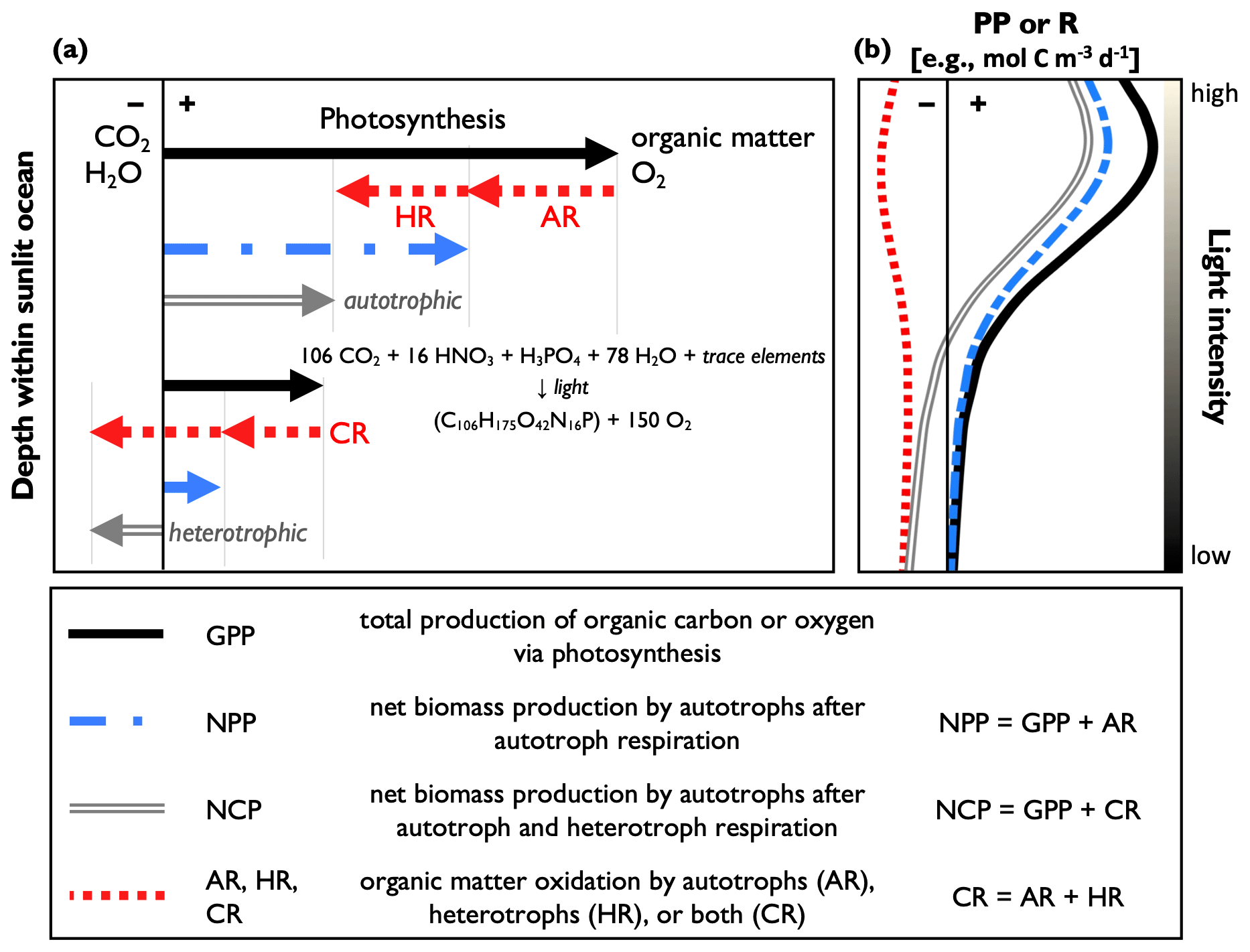
Figure 1A conceptual schematic and definitions of the common primary productivity (PP) and respiration (R) metrics: gross primary production (GPP); net primary production (NPP); net community production (NCP); and autotrophic, heterotrophic, and community respiration (AR, HR, and CR, respectively). Panel (a) shows simplified reaction equations of organic matter production and R. The upper part of the figure represents a region of net autotrophic conditions (NCP > 0), while the lower part represents a region of net heterotrophic conditions (NCP < 0). Panel (b) represents idealized PP and CR profiles, where PP declines with depth due to the light dependency of photosynthesis with a subsurface maximum resulting from photoinhibition. The vertical axis represents water column depth, and the thin black line divides positive and negative rates. The equation represents average oceanic aerobic photosynthesis, following Redfield nutrient stoichiometry. The reverse reaction represents respiration.
At the ecosystem level, PP can be quantified by the following common metrics: gross primary production (GPP), net primary production (NPP), and net community production (NCP) (Fig. 1). GPP measures community-wide photosynthesis, representing the total production of organic carbon or O2 by autotrophs (e.g., phytoplankton, cyanobacteria) and represents the photosynthetic energy available to the entire food web. GPP is reported as gross oxygen production (GOP) or gross carbon production (GCP), when defined in O2 or carbon equivalents, respectively. NPP refers to the net production of autotroph biomass when accounting for autotrophic respiration (i.e., organic matter oxidation; AR) and represents the amount of photosynthetically produced organic carbon available to heterotrophs (e.g., bacteria, zooplankton, fish). Lastly, NCP is the difference between GPP and respiration by autotrophs and heterotrophs (i.e., community respiration, CR) and therefore determines if an ocean region is net autotrophic (net production, indicated by NCP > 0) or net heterotrophic (net consumption and NCP < 0). When measured over sufficiently large temporal and spatial scales, NCP quantifies the amount of photosynthetically produced organic matter that is removed from the upper ocean (Laws 1991). GPP, NPP, and NCP are often expressed as volumetric equivalents of organic carbon or O2 production (e.g., mol C or ), and respiration terms are expressed in terms of organic C or O2 consumption. Accordingly, in a closed system, GPP, NPP, and CR can only have positive values, while NCP may assume positive or negative quantities.
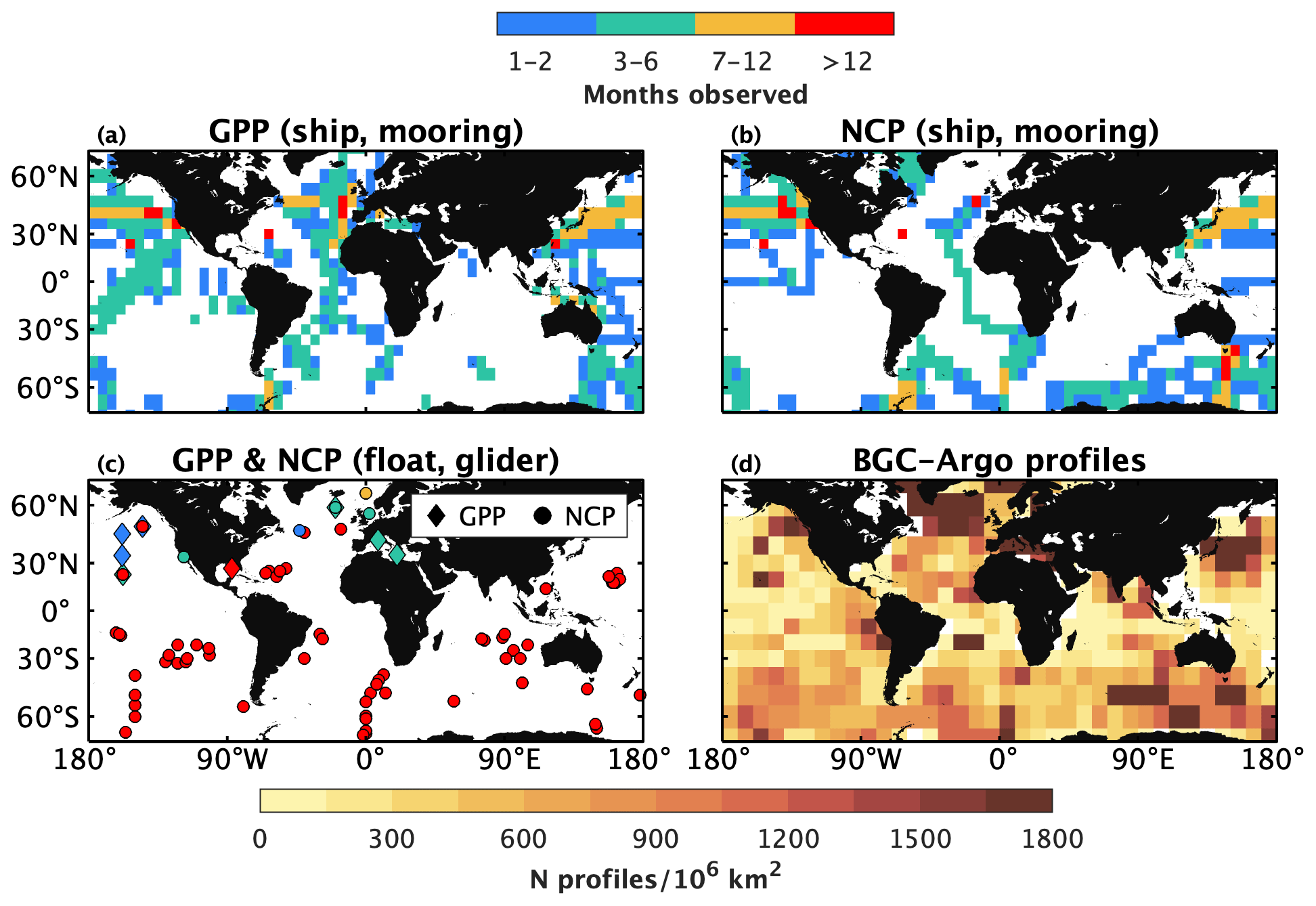
Figure 2Coverage of gross primary productivity (GPP) and net community productivity (NCP) datasets, as well as Biogeochemical-Argo (BGC-Argo) profiles. The upper row represents archived GPP and NCP data obtained from ships or moorings, while panel (c) shows the locations and durations of float- or glider-based GPP and NCP studies. Panel (d) shows a heatmap of the distribution of BGC-Argo profiles collected from 2010 through to 2022. Data in panels (a) and (b) were binned to a 5∘-by-5∘ grid. Only floats equipped with at least one biogeochemical sensor and registered in the international BGC-Argo programme were included in (d). A list of archived data sources is provided in Appendix A.
A variety of approaches and sampling platforms have been used to quantify PP. The earliest method estimates NCP and CR (and thus GOP) by measuring the evolution of O2 in natural seawater samples incubated in light and dark bottles, respectively (Gaarder and Gran, 1927). Other incubation-based approaches involve spiking samples with 14C- or 13C-labelled bicarbonate (GPP and NPP; Steeman Nielsen, 1952; Slawyk et al., 1977) or 18O-labelled water (GOP; Bender et al., 1987; Ferrón et al., 2016) to trace temporal changes in photosynthetic biomass or O2 production under realistic incubation conditions. These incubation approaches, though, are subject to various experimental biases, including containment effects on the plankton community, sensitivity to the incubation duration, and the excretion of labelled dissolved organic carbon (e.g., Pei and Laws, 2013; Cullen, 2001). The O2-to-argon (; Reuer et al., 2007; Spitzer and Jenkins, 1989) and triple O2 isotope (Luz and Barkan, 2000) methods thus emerged as tracer-based techniques for measuring PP from in situ observations and biogeochemical budget calculations. While the original incubation and tracer-based approaches have been applied widely, they require the collection of discrete samples from ships and therefore yield limited data coverage. Fortunately, advances in instrumentation have facilitated underway measurements of and particulates at the surface, giving rise to methods for high-resolution ship surveys of NCP and NPP, respectively (Tortell, 2005; Kaiser et al., 2005; Burt et al., 2018). Sampling via instrumented moorings similarly enabled high temporal resolution GPP and NCP time series at fixed positions (e.g., Emerson and Stump, 2010; Johnson, 2010; Weeding and Trull, 2014; Fassbender et al., 2016). Yet, while promising, these ship- and mooring-based approaches are subject to trade-offs between temporal, horizontal, and vertical measurement resolution. Moreover, many traditional approaches require expensive instrumentation (underway approaches) or considerable human oversight to collect the necessary data (incubation approaches), making them broadly inaccessible to the oceanography community or impractical for autonomous surveys. As a result of the challenges associated with the traditional PP methods, there are substantial gaps in PP datasets, with many ocean regions being undersampled or omitted from archived records (Fig. 2a and b). While satellite and statistical algorithms can provide PP estimates (Behrenfeld and Falkowski, 1997; Huang et al., 2021; Li and Cassar, 2016) with enhanced space–time coverage, their utility is constrained by limitations such as the accuracy of satellite ocean colour observations (e.g., Long et al., 2021) and the inability to detect subsurface information (Gordon and McCluney, 1975). Ultimately, the challenges associated with quantifying PP from the various in situ and ex situ methods has resulted in large uncertainties in global estimates of GPP and NCP. Reported estimates of GPP, for example, range from 8 to 14 Pmol C yr−1 (Westberry and Behrenfeld, 2014; Huang et al., 2021), while estimates of NCP and carbon export range from 250 to 2650 Tmol yr−1 (Boyd and Trull, 2007; Henson et al., 2011; Siegel et al., 2016; Westberry et al., 2012).
Considering the challenges associated with the above-mentioned traditional PP approaches, emerging methods that use autonomous profiler observations present a significant opportunity to expand the spatial and temporal coverage of PP datasets and improve satellite-based observations via hybrid approaches. The BGC-Argo programme, in particular, supports a growing array of profiling floats that provide continuous biogeochemical observations (e.g., O2, pH, nitrate, chlorophyll fluorescence, particle backscatter as a proxy for organic matter) in the upper 2000 m of the global ocean at ∼ 5 or 10 d intervals (Fig. 2d). The BGC-Argo fleet has grown steadily in recent years (> 500 operational floats as of Feb 2023), and the international community is targeting a sustained deployment of 1000 BGC floats distributed equally throughout the global ocean (Roemmich et al., 2021; Biogeochemical-Argo Planning Group, 2016). Several recent studies have quantified PP using BGC-Argo floats and other autonomous profilers, including gliders (see Table A1 in Appendix A and references therein), demonstrating the potential to derive year-round, depth-resolved PP estimates in remote ocean regions (Fig. 2c).
The primary objective of this paper is to demonstrate the potential of autonomous platforms, exemplified by BGC-Argo floats, for expanding the spatial and temporal coverage of PP estimates in the upper ocean. This paper explores float-based approaches for estimating GPP and NCP, since those methods are more mature than emerging approaches for NPP quantification (Arteaga et al., 2022; Yang, 2021; Estapa et al., 2019; Long et al., 2021). While recent literature has presented float-based methods for quantifying PP metrics in the interior ocean (e.g., Martz et al., 2008; Hennon et al., 2016; Arteaga et al., 2019; Su et al., 2022), the focus of this paper is on methods that resolve processes occurring principally within the euphotic zone. To facilitate a full exploitation of these new opportunities, we take stock of the float-based tools currently available to researchers and identify their strengths and limitations. After providing an overview of the emerging float- and glider-based PP approaches, we present quantitative analyses to demonstrate the current application of these methods, as single or combined tools. Overall, this paper is intended as a resource for a broad readership – including researchers who do not normally perform PP calculations – that summarizes the current state of GPP and NCP methods and helps to familiarize the community-at-large with the current benefits, challenges, and applications of these new tools.
This section provides an overview of approaches to quantifying GPP (measured as GOP and GCP) and NCP using observations made by BGC-Argo and other autonomous profilers. For each approach, we outline the premise and describe the specific variables used, sampling requirements, assumptions, and variations.
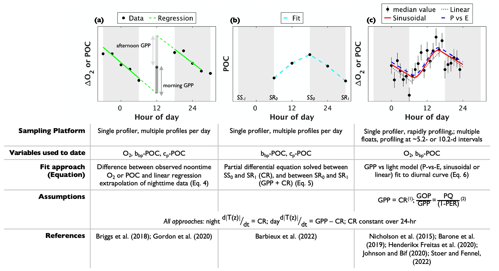
Figure 3Conceptual schematic of autonomous gross primary production (GPP) methods. The black markers in the figures represent oxygen anomaly (ΔO2) or particulate organic carbon (POC). In (a, b) markers represent data obtained using a single profiling platform, while those in (c) represent median (± standard deviation) data values during each hour of the day. The grey bars represent approximate nighttime periods between sunset (SS) and sunrise (SR) the following day. The lower part of the schematic summarizes the approach requirements. The “Variables used to-date” row identifies the tracers that have been used successfully, so far, under each method applied using autonomous profilers. It does not necessarily limit the respective float-based methods to those tracers, alone. Notes: (1) assumption applied in Nicholson et al. (2015), Johnson and Bif (2021), Stoer and Fennel (2023); (2) assumption applied in Stoer and Fennel (2023) only.
To date, autonomous GPP approaches have relied on measurements of O2 and particulate organic carbon (POC). NCP calculations have relied on O2, POC, and nitrate () measurements and estimates of dissolved inorganic carbon (DIC) and total alkalinity (TA). These tracers are selected because their concentrations in the sunlit ocean are impacted by primary production (photosynthesis and respiration). Other sources and sinks, such as exchange across the air–sea interface, vertical mixing, advection, and/or sinking and grazing, also impact the concentrations of these tracers. Accordingly, the temporal change in the concentration of a tracer, T, can be represented by the following general budget equation
where [T(t,z)] is the tracer concentration at time t and depth z, and is its time rate of change, expressed in concentration units per unit time (e.g., ). The left-hand side of the equation is measured, while terms on the right represent estimated quantities. Autonomous GPP methods interpret Eq. (1) over a 24 h period and are premised on the widespread observation of diurnal cycles in O2 and POC concentrations (Fig. 3). These cycles result from the dependency of photosynthesis on sunlight and are driven by daytime net autotrophic production (GPP minus CR) and nighttime CR (e.g., Siegel et al., 1989; Johnson et al., 2006). Assuming that diurnal variability in the other source/sink terms in Eq. (1) is negligible and that CR is constant over a 24 h period, Eq. (1) can be approximated by the following equation:
where T is O2 or POC. Given Eq. (2), vertically resolved GCP or GOP estimates can be derived if the diurnal cycles of POC or O2 in the euphotic zone are detectable.
Autonomous NCP approaches, in contrast, seek to interpret temporal changes in the concentration of a photosynthesis–respiration tracer over timescales exceeding 1 d (typically on the order of 1 week or more). Over these timescales, variability in the non-photosynthesis/respiration terms in Eq. (1) is not negligible. NCP (i.e., GPP+CR) is thus determined by rearranging Eq. (1), as follows, and estimating the contributions of the other source/sink terms to the observed tracer time series,
Equation (3) is typically evaluated at discrete time and depth intervals equivalent to the resolution of profiling measurements or by integrating quantities over coarser depth ranges (e.g., the mixed layer).
As GPP and NCP methods evaluate Eq. (1) over contrasting timescales, different sampling approaches have been employed to obtain the requisite tracer time series observations. For GPP calculations, multiple measurements per day are necessary to adequately resolve the diurnal cycle. Initially, GPP studies used a single profiling instrument, such as a glider (Nicholson et al., 2015; Barone et al., 2019), Lagrangian surface float (Briggs et al., 2018), or biogeochemical profiling float whose mission cycle was adjusted for frequent upper-ocean profiling (Barbieux et al., 2022; Gordon et al., 2020; Henderikx Freitas et al., 2020) (Fig. 3a and b). Gordon et al. (2020) and Barbieux et al. (2022), for example, used floats with profiling intervals of 3 and 6 h, respectively, to obtain diurnal cycle observations. The majority of the BGC-Argo fleet, however, collects a water column profile every ∼ 5 or 10 d. As a result, a diurnal cycle cannot be resolved using data from a single BGC-Argo float profiling at these intervals. This limitation was resolved by Johnson and Bif (2021) and Stoer and Fennel (2023), who quantified GOP and GCP from daily O2 or POC cycles using a composite of observations from multiple floats within selected geographic regions. To achieve roughly equal coverage of all hours of the day, they compiled data from floats that profiled at non-integer intervals (e.g., 10.2, not 10.0 d). Then, GPP was estimated by fitting the photosynthesis curve through all the resulting data points (as in Johnson and Bif, 2021) or by first calculating hourly median POC or O2 values (Stoer and Fennel, 2023) (Fig. 3c). Importantly, data from floats that do not sample all hours of the day evenly must be removed so that the resulting GPP estimates are not biased to a specific time of day. A non-integer sampling interval of 5.2 or 10.2 has been recommended to achieve approximately equal coverage of all hours over a float's lifecycle (Johnson and Bif, 2021; Stoer and Fennel, 2023). While GOP or GCP estimates derived from rapid profiling may yield daily temporal resolution (i.e., one GPP estimate per daily cycle) in ocean regions with strong diurnal variations, estimates derived from composite curves are more representative of typical conditions over the time and space scales that the data are composited. Sampling for NCP determinations has most commonly been based on nominal BGC-Argo profiling intervals, although high-resolution sampling using rapidly profiling floats is also feasible. Resulting NCP estimates have optimal vertical and temporal resolutions equivalent to those of the sampling profiling observations.
To estimate GOP, O2 is best expressed as a concentration anomaly, ΔO2, calculated as the difference between observed and equilibrium concentrations (i.e., ΔO2 = O2 − O2,equil; all typically mmol O2 m−3). Equilibrium concentrations are calculated using corresponding temperature and salinity observations (Garcia and Gordon, 1992). This practice is recommended to minimize potential diurnal solubility effects on . In NCP calculations, O2 is expressed as its absolute concentration. POC concentrations (typically mg m−3) for GCP and NCP calculations are derived from particle backscatter (bbp) or beam attenuation (cp, typically at 660 nm) measurements (both m−1) using regional algorithms (e.g., Loisel et al., 2011; Cetinić et al., 2012) or those derived from latitudinally distributed datasets (e.g., Graff et al., 2015, based on data obtained from the Atlantic Meridional Transect and equatorial Pacific) (see Table A4 for a list of selected POC algorithms). Many algorithms estimate POC from bbp at 700 nm (bbp,700), which is the wavelength that is most commonly measured by BGC-Argo floats. For algorithms that rely on different bbp wavelengths (e.g., bbp at 470 nm, as in the algorithm of Graff et al., 2015), a power-law equation is required to convert between bbp,700 and bbp at other wavelengths (Boss et al., 2013; Boss and Haëntjens, 2016). Only a subset of floats directly measures bbp,470 or cp,660. Lastly, because TA and DIC are not directly measured by BGC-Argo floats, NCP estimates derived using those variables rely on calculations of their concentrations using float measurements and an empirical TA function (Huang et al., 2022). Total alkalinity is estimated from float pH, O2, and hydrographic observations using a neural network algorithm (e.g., Bittig et al., 2018; Carter et al., 2021), and DIC is subsequently calculated from float pH and derived-TA based on known seawater carbonate system relationships (Gattuso et al., 2022).
2.1 GPP
Given a diurnal POC or O2 time series, GCP or GOP have been estimated using three different mathematical algorithms that describe the shape of the diurnal curve. Two of the approaches have been applied only using single profilers making multiple measurements of the upper ocean each day; the other has been adapted for composite daily cycles (Fig. 3). Each method yields one daily GPP estimate per diurnal curve, and estimates may be vertically resolved or integrated, depending on the sampling infrastructure used. As a result, the spatial and temporal resolution of the following methods is constrained by the measurement resolution of the float or glider.
Briggs et al. (2018) described a method that requires estimating tracer sink terms (including CR) by fitting a type I linear regression to nighttime (sunset to sunrise) POC or O2 data (red line in Fig. 3a). Extrapolating the regression line from the POC or O2 value at sunrise (sunset) to noon on the following (preceding) day (dashed line in Fig. 3a) then yields an estimate of the tracer's midday concentration in the absence of photosynthesis. The difference between observed noontime concentrations ([T(t,z)]observed) and the value predicted by the regression extrapolation ([T(t,z)]predicted) is an indication of GPP, so that GPP is calculated as follows:
Daily GPP is taken as the average of morning and afternoon values. This method has been applied by constructing diurnal O2 or cp-POC cycles from continuous, upper-ocean observations using a Lagrangian surface float (Briggs et al., 2018) or from a float profiling at 3 h intervals (Gordon et al., 2020). In both cases, surface layer-integrated GPP estimates were obtained by integrating O2 or POC observations within a density-defined layer. A minimum upper-ocean sampling resolution of ∼ 3–4 h is likely necessary to obtain a robust nighttime regression fit to the data and to derive GPP at daily resolution.
Barbieux et al. (2022), following Claustre et al. (2008), introduced another approach for GCP derivations from a rapidly profiling BGC-Argo float deployed in the Mediterranean Sea. In their method, GCP is estimated by solving the following differential equation for the time rate of change in depth-resolved POC concentrations:
where μ represents autotrophic growth, and L represents particle losses due to CR, sinking, and grazing (both d−1). Equation (5a) is a variation of Eq. (2), where and are equivalent to GPP(t,z) and CR(t,z), respectively. Integrating Eq. (5.1) between sunset (SS0) and the following sunrise (SR1), when μ=0, yields an estimate for the loss term,
Combining Eqs. (5.1) and (5.2), assuming constant L(z), and integrating over a full day (sunrise to sunrise; SS0 to SS1) produces the following equation for daily GPP:
where the index i represents time-resolved POC measurements from sunrise on the first day (SR0) to sunrise on the following day (SR1) (Fig. 3b). Barbieux et al. (2022) used a BGC-Argo float profiling at 6 h intervals, thus enabling GCP calculations with daily resolution. POC quantities were integrated vertically in three upper-ocean layers.
A third approach for estimating GPP has been applied successfully using O2 observations from gliders (Nicholson et al., 2015; Barone et al., 2019), a rapidly profiling BGC-Argo float (Henderikx Freitas et al., 2020), and a composite of O2 and bbp-POC cycles from BGC-Argo floats (Johnson and Bif, 2021; Stoer and Fennel, 2023). In this method, introduced by Nicholson et al. (2015), Eq. (2) is rewritten to describe discrete, time-dependent changes in POC or O2 as a function of time-variable irradiance, E(t):
given and where and t1−t0 are the mean daily irradiance level and time step, respectively. The middle term, , represents photosynthesis as a function of time-varying irradiance, which is calculated from geospatial (location and time) data. A photosynthesis-versus-irradiance (P-vs-E) relationship, a sinusoidal function, and a linear algorithm have been proposed for (see coloured lines in Fig. 3c), although resulting GPP estimates are not statistically different across models (Barone et al., 2019; Henderikx Freitas et al., 2020). Given time-resolved ΔO2 or POC observations, Eq. (6) can be re-expressed as a system of linear equations (see Eq. 4 in Barone et al., 2019), and GPP and CR are approximated as the least-square coefficients required to fit to the observed diurnal cycle. MATLAB code for solving the system of linear equations has been provided by Barone et al. (2019) and modified by Johnson and Bif (2021). Stoer and Fennel (2023) modified the code further and adapted it for Python.
To simplify the system of equations, Nicholson et al. (2015), Johnson and Bif (2021), and Stoer and Fennel (2023) assumed equivalency between daily integrated GPP and CR. Although the assumption is physically invalid in many ocean regions since it may unrealistically constrain daily NCP to zero, it enables calculations of statistically robust GPP estimates in ocean regions where diurnal oscillations are small. Barone et al. (2019), in contrast, calculated separate GPP and CR values, albeit with larger errors in each term. Similarly, Gordon et al. (2020) attempted separate GPP, CR, and NCP estimates by applying the Briggs et al. (2018) method for float data collected from the Gulf of Mexico.
Surface layer-integrated GOP has been derived by applying this approach to observations obtained from gliders (Nicholson et al., 2015; Barone et al., 2019) or rapidly profiling floats (Henderikx Freitas et al., 2020). In principle, these sampling methods can yield daily diurnal curves and GOP estimates. In practice, however, the resulting GOP values may have an effective temporal resolution of ∼ 5–7 d in low-productivity regions, due, in part, to limited detection (i.e., low signal-to-noise ratio) of daily O2 oscillations (Barone et al., 2019). Johnson and Bif (2021) and Stoer and Fennel (2023) extended the present approach for composite sampling, exploiting the broader BGC-Argo array. Johnson and Bif (2021) collated float ΔO2 data in different geographic regions between 2010 and 2020, constructing vertically resolved diurnal cycles by binning the composited datasets in 10 m intervals, and averaging values to the nearest local hour. GPP is calculated for a single composited diurnal curve, as described above. Stoer and Fennel (2023) further extended the approach by calculating GCP from bbp-POC and using observations median-binned to each local hour. Using data from a meta-analysis by Moran et al. (2022), they calculated an average percent extracellular release (PER) to account for dissolved organic carbon (DOC) production not detected by the bbp sensor. Accordingly, they scaled their GCP values using the calculated PER value and converted between GCP and GOP using a photosynthetic quotient (PQ) value of 1.4, i.e., . Finally, Johnson and Bif (2021) and Stoer and Fennel (2023) derived NPP from the diurnal GPP calculations by applying a global empirical GOP:NPP ratio of 2.7 mol O2 (mol C)−1 (i.e., ).
The horizontal and temporal resolution of the present approach based on composited sampling is limited by the number of floats and profiles in a given geographic region. There must be enough profiles taken equally throughout the day to distinguish a daily signal. Johnson and Bif (2021) estimated that a minimum of 20 and 50 O2 profiles in each hour (equivalent to 480 to 1200 profiles, per day) are required to clearly detect diurnal variability in tropical and high-latitude waters, respectively. For the region 30–70∘ S, Stoer and Fennel (2023) estimated that at least 2000 bbp and 5000 O2 profiles, per diurnal curve, are required to limit the noise-to-signal ratio of the resulting PP estimates to one or less.
Table 1Variations in budget terms used in float- and glider-based net community productivity (NAP) calculations at Ocean Station Papa.
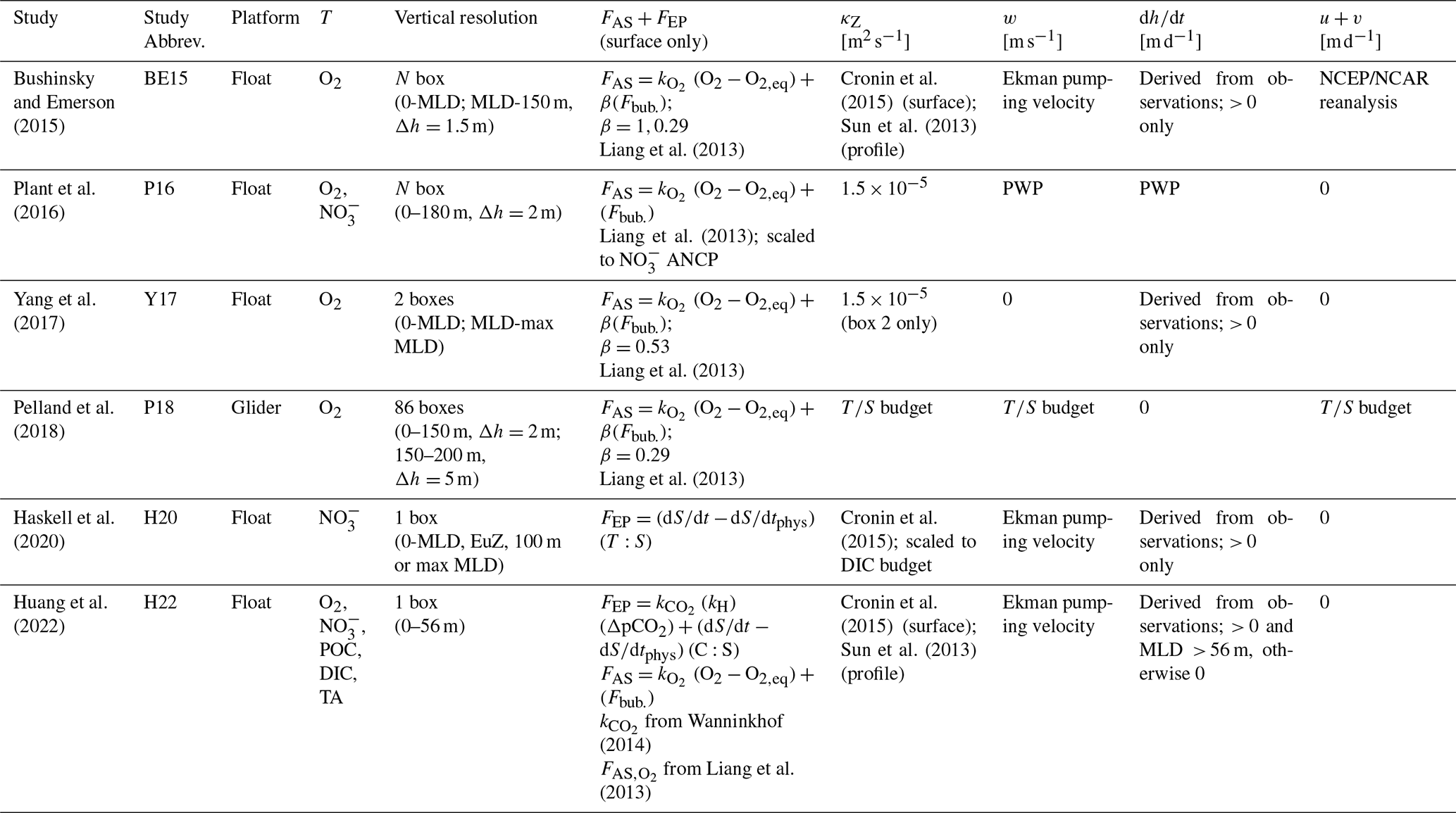
O2 = oxygen concentration (mol m−3); POC = particulate organic carbon concentration (mol m−3); = nitrate concentration (mol m−3); DIC = dissolved inorganic carbon concentration (mol m−3); TA = total alkalinity (mol m−3); MLD = mixed layer depth; FAS = air–sea gas exchange (); Fbub = air–sea bubble flux (); FEP = evaporation or precipitation (); and = air–sea gas transfer coefficient for O2 and CO2; κZ = eddy diffusivity coefficient [m2 d−1]; w = vertical advection velocity [m d−1]; = change in layer depth [m d−1]; u+v = horizontal advection velocities [m d−1]; Δh = box vertical displacement ( in Eq. 7); β = bubble-mediated transfer scaling coefficient [unitless]; PWP = Price–Weller–Pinkel mixed layer model (Price et al., 1986); C:S = observed DIC : salinity ratio [mol C:S]. “Surface” refers to values derived in the mixed layer only, while “profile” is for values derived over the full water column.
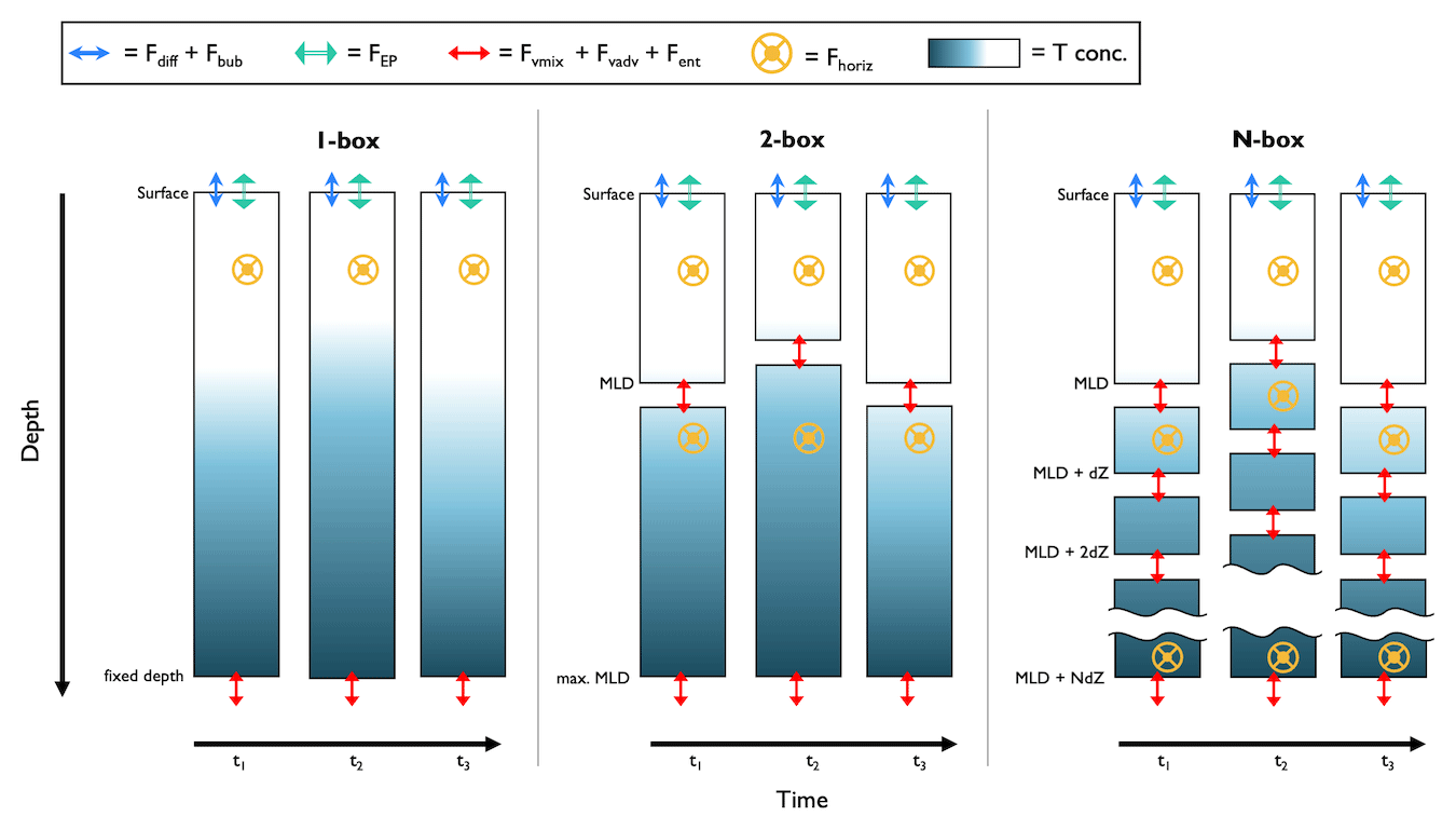
Figure 4Schematic of box model setups for float-based NCP approaches. The columns represent a profile of tracer concentration at discrete time intervals (tn, where n is the nth point in time), and the rows are divided into vertical layers (dZ). Tconc = tracer concentration; MLD = mixed layer depth; Fdiff = air–sea flux via diffusion; Fbub = air–sea flux via bubbles; FEP = evaporation or precipitation flux; ; Fvmix = vertical transport flux via diapycnal mixing; Fvadv = vertical transport flux via advection; Fent = vertical transport flux via entrainment; and Fhoriz = horizontal transport flux.
2.2 NCP
Autonomous NCP methods invoke a different set of calculations and assumptions than GPP methods. Namely, the sum of non-biological terms (i.e., physical fluxes) is estimated and subtracted from observed tracer changes in discrete time and depth intervals (as in Eq. 3). Equation (3) is commonly solved using a one- or two-dimensional box model approach by partitioning the water column into layers (e.g., mixed layer, euphotic zone) or by discretizing in depth intervals (Table 1; Fig. 4) and performing calculations between consecutive profiles (e.g., dt in Eq. (3) is the float profiling interval) or as seasonally integrated quantities (e.g., Baetge et al., 2020). The following equation describes the calculations performed at each time step and in each depth layer:
NCP(t,z) (typically ) represents NCP integrated over the depth range (m). [T(t,z)] is the average tracer concentration between hi and hi+1, and is the observed change in the tracer's concentration between time intervals (both ). Lastly, ΣF is the sum of the estimated physical fluxes and non-NCP biological terms (). Integrating the resulting NCP values over 1 year provides an estimate of annual net community production (ANCP; ), which is equivalent to carbon export when integrated to the depth of the maximum annual mixed layer (Yang et al., 2017). However, the depth to which NCP and ANCP estimates are integrated impacts the interpretation and magnitude of the resulting NCP values and metabolic state of the system. Haskell et al. (2020), for example, reported ∼ 10 %–20 % variability in climatological ANCP and monthly NCP estimates calculated down to the seasonal mixed layer depth (MLD), euphotic zone, 100 m, and annual maximum MLD. Pelland et al. (2018) noted ∼ 50 % variation in ANCP values when integrating to the seasonal MLD versus 120 m. Ship-based work has also demonstrated the sensitivity of export estimates to the depth of wintertime ventilation, with regions of deep winter MLDs experiencing greater ventilation and therefore reduced export or ANCP calculated to that depth (Palevsky et al., 2016).
The general approach represented by Eq. (7.1) has been applied using float-based O2, , DIC, TA, and POC, although there is significant variability in how and which physical fluxes are included when calculating ΣF and in how the box model is discretized in time and space (Table 1). Air–sea gas exchange (gases only), vertical and lateral exchange, or transport and evaporation/precipitation (excluding O2) are important processes that modify tracer concentrations over daily to monthly timescales (Bushinsky and Emerson, 2015; Emerson and Stump, 2010; Huang et al., 2022; Pelland et al., 2018). Accordingly, ΣF is estimated by calculating some or all of the terms in the following equation:
FAS represents gas exchange via bubbles (Fbub) and diffusion (Fdiff) at the air–sea interface; FEP is the evaporation/precipitation flux at the surface; are vertical transport via diapycnal mixing, advection, and entrainment, respectively; and Fhoriz is horizontal transport. Fbio represents biological processes, not including NCP, such as particulate inorganic C production/consumption, DOC production, or POC sinking, which are reflected in the DIC, TA, and POC budgets (Huang et al., 2022). The general equations for the physical terms in Eq. (7.2) are as follows.
where k is the wind-speed-dependent diffusive gas transfer coefficient (m d−1), [T]eq is the temperature- and salinity-dependent equilibrium concentration at ambient sea level pressure (mol T m−3), and Fc and Fp represent bubble-mediated gas transfer via small and large bubbles, respectively. The β term is a bubble-flux tuning coefficient between 0 and 1. The evaporation/precipitation term (Eq. 7.5) is typically estimated by normalizing tracer concentrations to the observed salinity during each time step and multiplying by the measured time-dependent change in salinity (Fassbender et al., 2016; Huang et al., 2022). In Eq. (7.5), T:S is the ratio of tracer T to salinity, is the observed change in salinity over time, and is the change due to physical processes. Fdiff, Fbub, and FEP are zero below the surface box. The transport terms κZ (m2 d−1), w, , u, and v (all m d−1) represent the diapycnal eddy diffusivity coefficient, vertical advection velocity, the rate of change of a given depth layer, and the lateral advection velocities, respectively. (mol m−4) is the vertical gradient between consecutive depth bins, while Δ[T]z, Δ[T]x, and Δ[T]y (all mol m−3) represent concentration differences in vertical and horizontal directions. Importantly, when evaluating NCP following Eq. (7), it is assumed that the float remains in a single water mass, such that tracer changes strictly represent temporal variations due to NCP and the processes described in Eqs. (7.3)–(7.9). In reality, however, this may not always be the case, and the resulting effect on NCP calculations remains a source of uncertainty that is difficult to constrain.
As summarized in Tables 1 and A3, different studies have represented the terms in Eqs. (7.3)–(7.9) in different ways. Parameterizations of air–sea exchange (Eqs. 7.3–7.4) and diapycnal mixing (Eq. 7.6) vary most widely across studies, and those fluxes typically contribute the largest source of uncertainty in budget-based NCP and ANCP calculations, up to ∼ 40 % and 20 %, respectively (Bushinsky and Emerson, 2015; Yang et al., 2017; Huang et al., 2022). Different Fdiff+Fbub parameterizations, for example, have been employed, and efforts have been made to tune those terms for local conditions using a scaling coefficient (β). Yang et al. (2017) and Emerson et al. (2019) tuned Fc+Fp for Ocean Station Papa (OSP) by minimizing differences between observed mixed-layer N2 concentrations and values predicted by the same mass balance used for their O2-based ANCP calculations. Plant et al. (2016) tuned Fbub by scaling the magnitude of that flux to minimize differences between O2- and -based ANCP estimates. Most recently, Yang et al. (2022) introduced a correction for air–sea flux estimates that relies on reanalysis data products to account for small temperature differences in the ocean skin (the ∼ 500 µm thick layer over which gas exchange occurs) and mixed layer which impact the magnitude of diffusive and bubble-mediated gas exchange. Only that paper and a subsequent one by Emerson and Yang (2022) have applied the correction, but its influence on ANCP estimates may be as large as ∼ 40 %. Approaches to estimating the diapycnal mixing flux also differ widely across studies. Most invoke values from the literature, either selecting constant or time-varying climatological κZ values for the study region. Bushinsky and Emerson (2015) and Huang et al. (2022) used an average OSP κZ time series from Cronin et al. (2015) for the base of the mixed layer and scaled values vertically to a background of 10−5 m2 s−1 below the thermocline, following Sun et al. (2013). Haskell et al. (2020) scaled the Cronin et al. (2015) κZ climatology for their NCP model by minimizing differences between - and DIC-based ANCP estimates. These approaches, however, are somewhat problematic as they likely neglect significant spatial and temporal variability in upper-ocean mixing rates. Pelland et al. (2018) derived independent estimates of all the transport terms (κZ, w, u, v) by using their glider observations to close heat and salt budgets for OSP, while Plant et al. (2016) estimated the physical transport terms by running locally forced simulations of a Price–Weller–Pinkel (PWP) mixed layer model (Price et al., 1986). Other studies have estimated vertical advection velocities (u) by calculating the Ekman pumping velocity from local wind stress data. Most float-based approaches neglect horizontal transport, suggesting its influence on NCP estimates would be small away from boundary currents, eddies, or frontal zones, and over seasonal timescales or longer (e.g., Yang et al., 2017; Huang et al., 2018). Emerson and Bushinsky (2015) is the only float-based study to have calculated that term, and they found it to be small relative to the vertical physical fluxes, contributing < 7 % to uncertainty in their ANCP estimates. In a glider-based study, however, horizontal advection fluxes were larger than the sum of all vertical fluxes in the upper 120 and 200 m of the water column (e.g., Pelland et al., 2018). Lastly, entrainment terms, which are often estimated from observed changes in the mixed layer depth or other depth horizons between time intervals, tend to be small, except during periods of rapid mixed layer depth changes.
Different approaches to setting up the vertical discretization have been also applied. For example, Bushinsky and Emerson (2015), Plant et al. (2016), and Pelland et al. (2018) divided the upper water column into multiple depth layers with ∼ 1.5–5 m vertical resolution. Other studies have employed coarser one- or two-box model frameworks, partitioning the upper water column into layers defined by the seasonal or winter maximum mixed layer depth (MLD), euphotic depth, or a fixed density or depth horizon (e.g., Yang et al., 2017; Haskell et al., 2020; Huang et al., 2022). In all cases, the vertical transport and mixing flux terms are evaluated by measuring the depth-dependent change in or ΔTZ) across the base of each box (Fig. 4), and air–sea exchange and/or evaporation are quantified at the top of the surface box, only. There is no consensus on the optimal vertical discretization scheme, and no estimates of the (A)NCP sensitivity to the approach have been reported.
By performing simultaneous NCP calculations using multiple tracers, it is possible to partition biological productivity into distinct biogenic pools and to estimate other non-NCP biological terms (Fbio in Eq. (7.2); Haskell et al., 2020; Huang et al., 2022). For example, while calculations based on O2 and target particulate and dissolved organic C cycling, those based on DIC or TA are also influenced by inorganic C cycling associated with non-NCP production of calcareous shells by some organisms (Fassbender et al., 2016). Calculations from POC represent only the particulate organic fraction, as well as POC sinking. As a result, differences between DIC, TA, POC, and O2- or -based estimates can be used to quantify sinking rates, as well as the relative importance of particulate organic, dissolved organic, and particulate inorganic production within a system (see details in Huang et al., 2022).
Finally, while most NCP studies to date have performed the above calculations at the approximate resolution of the profiling instrument, a handful of studies have evaluated NCP by integrating tracer changes over seasonal timescales (Table A1). Johnson et al. (2017b), Bif and Hansell (2019), and Baetge et al. (2020) all estimated NCP as the winter-to-summer drawdown of in the upper 100, 75, and 200 m, respectively, neglecting any other sources or sinks (i.e., , , and ΣF=0 in Eq. 7.1). A reference winter profile is taken from float observations, and drawdown is converted to C or O2 equivalents using Redfield stoichiometry.
Here, we summarize and demonstrate, through examples, the current capacity to determine GPP and NCP using the BGC-Argo array. The main goal of this section is to provide readers with an overview of how the emerging float-based methods are applied. Sections 3.1 and 3.2 demonstrate the methods' applications at local and basin-to-global scales, respectively. In Sect. 4, we discuss the current challenges and opportunity to further broaden the scope of GPP and NCP calculations using floats.
3.1 GPP and NCP calculations at local scales
To date, a handful of studies have examined GPP and NCP dynamics at relatively small spatial scales, using data from one or several floats deployed within a single geographic region. Targeted GPP studies employing single BGC-Argo (or BGC-Argo-like) floats have only occurred in the Mediterranean Sea (Barbieux et al., 2022), N Pacific (Henderikx Freitas et al., 2020), and Gulf of Mexico (Gordon et al., 2020). Gordon et al. (2020), however, were unable to reliably determine GOP from their diurnal O2 curves due to low biological productivity and confounding signals from physical O2 fluxes. While Barbieux et al. (2022) successfully derived an approximately 4-month euphotic-zone integrated GCP time series in two locations in the Mediterranean Sea using cp-POC data, diurnal variations in the bbp-to-POC relationship precluded the same calculations using bbp-POC data.
Float-based NCP studies are somewhat more numerous than GPP studies (Table A2) but are similarly limited in their geographic extent. NCP has been well-studied around Ocean Station Papa (OSP; 50∘ N, 145∘ W) in the subarctic NE Pacific (Sect. 3.1.1), and only a handful of localized studies have occurred elsewhere, such as in the South China Sea (Huang et al., 2018) and the NW Atlantic (Alkire et al., 2014; Yang et al., 2021) (Fig. 2c). These studies have spanned from about 1 year to several years and have employed single floats or multiple floats clustered within the same region. Plant et al. (2016), for example, used float data from six floats that were deployed independently and consecutively between 2008 and 2013.
Several float-based studies have quantified ANCP in the Southern Ocean; however, that work has principally focused on processes occurring below the euphotic zone (e.g., Martz et al., 2008; Hennon et al., 2016; Arteaga et al., 2019; Su et al., 2022)
No single study has examined NCP and GPP dynamics simultaneously, although Alkire et al. (2014, 2012) and Briggs et al. (2018) studied NCP and GPP during the same NW Atlantic spring bloom in their respective papers.
3.1.1 NCP case study at OSP
Ocean Station Papa is one of longest-running time series with sustained oceanographic observation. In the past 20 years, the monitoring site has seen several deployments of Biogeochemical-Argo floats and profiling gliders, allowing for various studies to estimate NCP. To demonstrate the current abilities to calculate NCP for studies at a local scale, we performed a case study analysis of studies that utilized float/glider data to estimate NCP at OSP. A similar analysis is not presently feasible for GPP, owing to the small number of localized studies using floats and gliders and the currently insufficient number of profiles available to conduct GPP calculations from composite diurnal cycles. Indeed, there have not been enough published float-based GPP studies to date in a single region to compile those data and perform an analysis similar to the present NCP analysis. Moreover, we could not perform our own local GPP calculations due to the large number of profiles required to make those calculations. These factors currently preclude an analogous analysis of GPP methods at localized scales.
We compiled all available published float and glider NCP data collected from OSP between 2008 and 2020. The published data constitute five independent studies, each employing slightly different approaches to quantifying NCP and ANCP (Table 1). For comparison with the profiler data, we also compiled independent NCP estimates from ship-board sampling, moorings, and satellites collected over the same time frame as the float/glider data. We present time-explicit, seasonal average, and annually integrated NCP values integrated to the depth of the annual maximum winter mixed layer (typically ∼ 120 m at OSP), and we present depth-resolved seasonal average NCP. All values were converted to O2 equivalents using a PQ of 1.4, and O2 : ratio of 150 : −16. Data sources and a detailed description of our data handling are provided in Appendix A (Table A1).
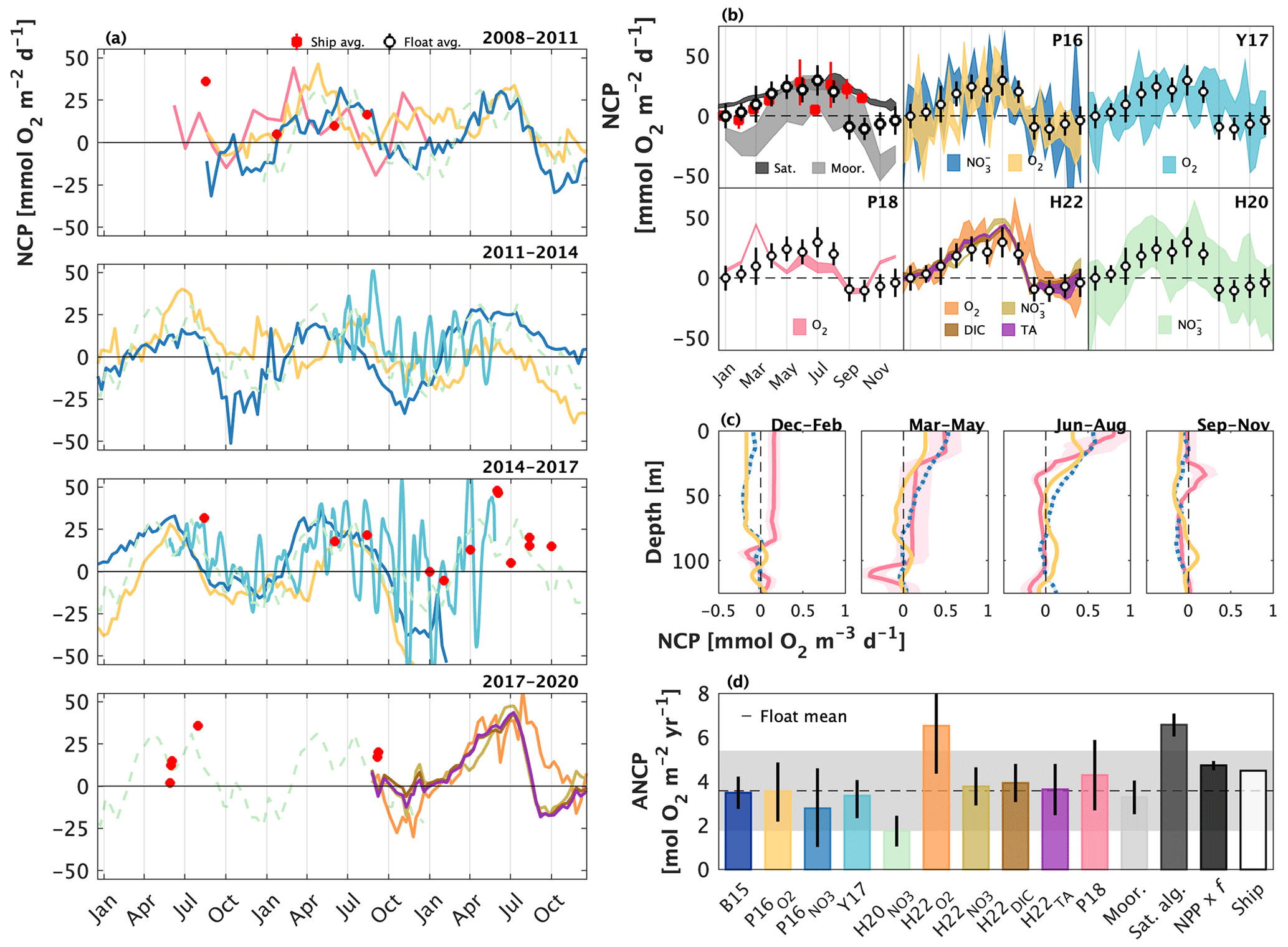
Figure 5Published float- and glider-based net community production (NCP) estimates from Ocean Station Papa (OSP) located at 50∘ N and 145∘ W. (a) Full time series NCP. Red markers are ship-based estimates. The Haskell et al. (2020; H20) record (light green) is dashed because it represents an average annual cycle between 2009 and 2018. (b) Average seasonal cycles, presented at the temporal resolution of each study. Shading around the mean represents the reported approach uncertainty or the standard deviation of estimates derived over multiple years. The black and red markers and error bars represent the average ± 1 standard deviation annual cycle derived from float and ship sampling, respectively. Depth-resolved NCP estimates in (c) are from Plant et al. (2016; P16) and Pelland et al. (2018; P18). (d) Annually integrated NCP (ANCP), including data from mooring studies (Emerson, 2010, 2014; Fassbender et al. 2016; Haskell et al., 2020), a satellite algorithm (Li and Cassar, 2016), a combination of satellite net primary productivity (NPP) and an empirical estimate of the ratio of carbon export to NPP (or the f ratio) (Westberry et al., 2008; Laws et al., 2011), and ship-based sampling. Colours in (a–c) correspond with labels in (b, d). Values in panels (a), (b), and (d) represent quantities integrated to the annual maximum mixed layer depth. The subscripts (e.g., ) denote the tracer used in each study. Y17 = Yang et al. (2017); H22 = Huang et al. (2022).
The compilation of float and glider data from OSP yields a nearly continuous 12-year time series of NCP and ANCP estimates and a shorter 7-year time series of depth-resolved estimates (Fig. 5). The temporal resolution of estimates ranges from 10 d (float profiling interval; Plant et al., 2016; Huang et al., 2022) to 1 month (Pelland et al., 2018). Yang et al. (2017) provided NCP estimates interpolated to 1 d resolution, while data provided by Haskell et al. (2020) were averaged over 6 years. The depth-resolved data from Plant et al. (2016) and Pelland et al. (2018) had vertical resolutions of 2 and 2–5 m, respectively.
There is general consistency in the magnitude (NCP, ANCP) and seasonal patterns (NCP) across the float and glider studies. Most datasets, for example, reveal peak productivity and autotrophy (NCP > 0) between June and August and minimum values and heterotrophy (NCP < 0) between November and February (Fig. 5a and b). These patterns are also broadly consistent with those of the independent data records. Indeed, the average seasonal float NCP cycle is very similar to the average of ship-based measurements between January and July (compare white and red markers in Fig. 5b), and the seasonality is similar to the average estimates derived from moorings and satellites. Notably, while all float/glider approaches consistently predict periodic net heterotrophic conditions, the satellite-based approaches only ever produce positive NCP estimates, reflecting how those algorithms are trained using only positive PP data (Li and Cassar, 2016; Westberry et al., 2008; Behrenfeld and Falkowski, 1997).
The float/glider ANCP estimates are typically within 1 standard deviation of one another (Fig. 5d). Exceptions to this result are the Huang et al. (2022) O2-based estimate and the Haskell et al. (2020) -based estimate. It is, however, somewhat unsurprising that the Huang et al. estimate exceeds the others, because ANCP values from that publication were integrated only to 50 m depth (i.e., calculations integrated to the annual maximum MLD were not available) and may thus exclude subsurface regions of net heterotrophy which occur during the autumn and winter (Fig. 5c). For the same reason, it is not surprising that the float and glider ANCP estimates are typically lower than estimates derived from moorings (Fassbender et al., 2016; Emerson and Stump, 2010), satellites, and ships, which only resolve a narrow depth range in the upper ocean.
Despite the general agreement across float and glider NCP approaches, there are some important differences, which are particularly apparent in the full, time-resolved NCP record (Fig. 5a). For example, NCP estimates made at the same time diverge by up to ∼ 50 , and in extreme cases by ∼ 100 across different approaches (Fig. 5a). Likewise, the spread in average seasonal NCP values is ∼ 50 (Fig. 5b). The most notable difference across studies is the anomalous phenology of the Pelland et al. (2018) record, which identifies peak NCP in March and net heterotrophy in September and October, only. These differences are also seen in the depth-resolved record from that publication. Interestingly, however, the anomalies in the seasonal record of Pelland et al. (2018) do not correspond with anomalous ANCP.
Despite these differences, our analysis demonstrates strong agreement across different float-based NCP studies and illustrates the capacity to derive NCP time series using consecutive float deployments. In Sect. 4.2, we discuss the factors that contribute to differences in the NCP results presented in Fig. 5.
3.2 GPP and NCP calculations on basin and global scales
Few studies have examined PP at basin or global scales using float data. Johnson and Bif (2021) provided the first global assessment of decadal GOP and NPP derived from a compilation of float observations, while Stoer and Fennel (2023) presented float-based GPP and NPP estimates of the Southern Hemisphere ocean. Both studies performed depth-resolved and euphotic zone-integrated calculations by subsetting all available BGC-Argo O2 and/or bbp-POC data into different geographic regions. Johnson and Bif (2021) performed calculations in 10∘ latitude bands in the Northern Hemisphere and Southern Hemisphere, subdividing the data into annual and bimonthly segments. They also performed calculations at 2-monthly intervals around the Bermuda Atlantic Time-series Study station and Hawaii Ocean Time-series sites. Stoer and Fennel (2023), in contrast, performed calculations between 30 and 70∘ S, only, due to an insufficient number of bbp profiles north of that region at the time.
No studies to date have estimated global NCP from floats. Two Southern Ocean studies (Johnson et al., 2017b; Huang et al. 2023) and two subtropical ocean studies (Yang et al. 2019; Emerson and Yang, 2022) have, however, provided extensive assessments of (A)NCP from a compilation of multiple floats. Johnson et al. (2017b) used BGC-Argo data to characterize ANCP in the Southern Ocean by compiling data from 24 floats deployed between 2009 and 2016. Similarly, Huang et al. (2023) provided basin-scale estimates of NCP in different biogenic carbon pools in the Southern Ocean, derived using a compilation of floats and multiple tracers (DIC, TA, , POC). Yang et al. (2019) and Emerson and Yang (2022) compiled O2 data from multiple floats to estimate ANCP in the North Hemisphere and South Hemisphere subtropical ocean. Lastly, some recent work (e.g., Martz et al., 2008; Hennon et al., 2016; Arteaga et al., 2019; Su et al., 2022) compiled data from subsets of the Southern Ocean BGC-Argo array to quantify ANCP and respiration below the euphotic zone.
No work has simultaneously characterized NCP and GPP at global or regional scales using BGC-Argo data.
3.2.1 Global GPP case study
Building on recent work by Johnson and Bif (2021) and Stoer and Fennel (2023), we performed new global GOP and GCP calculations using the available BGC-Argo array. We summarize those calculations here and provide further details in Appendix A. Presently, a similar analysis is not feasible for NCP, as global-scale NCP calculations have not yet been attempted by the community, and only a small handful of studies have calculated NCP at basin scales (see Sect. 3.1). As a result, intercomparisons of published results at these scales are not feasible, and new calculations of global NCP are beyond the scope of the present paper.
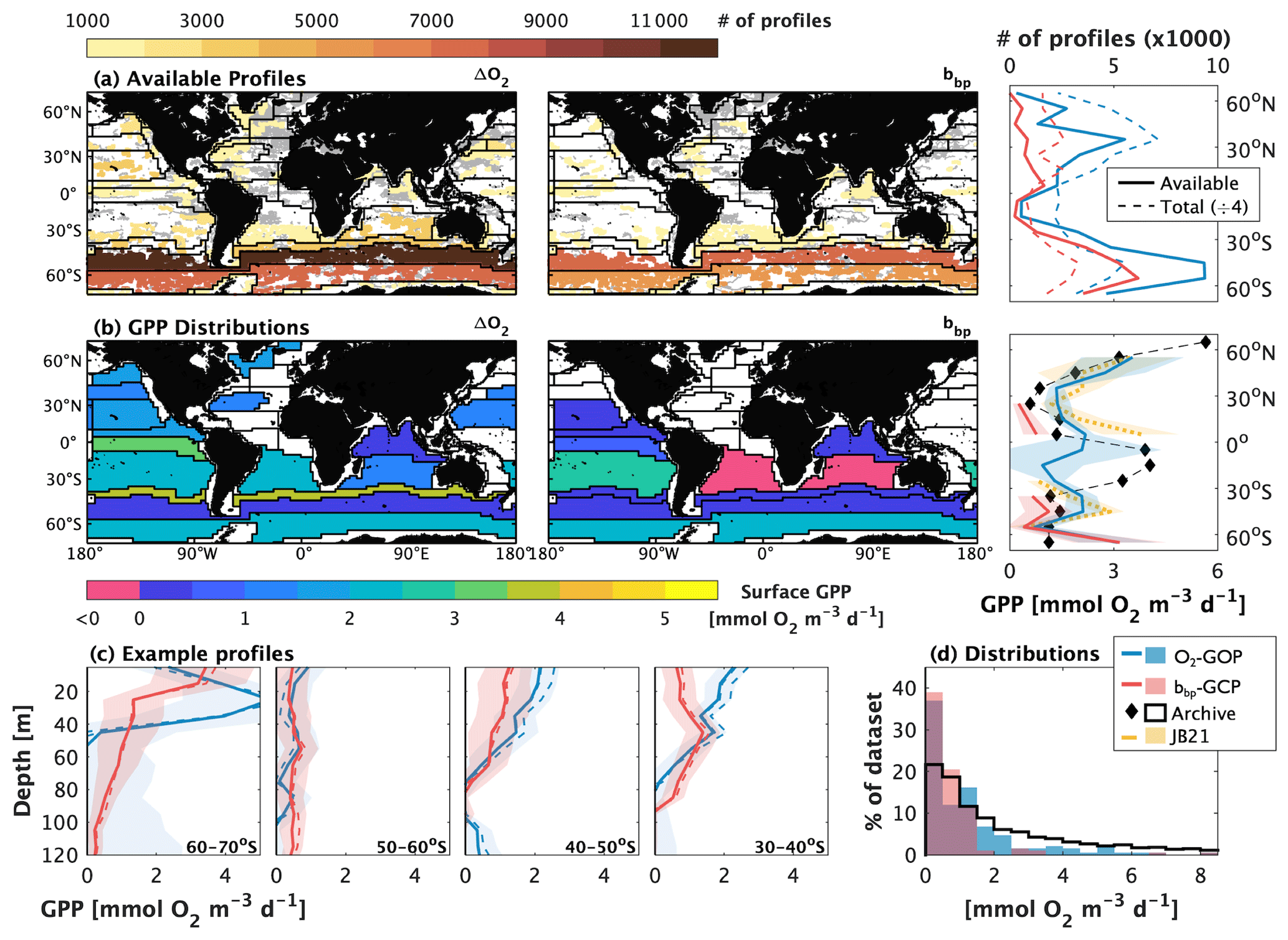
Figure 6Demonstration of global-scale float-based gross oxygen productivity (GOP) and gross carbon productivity (GCP) estimates. Panel (a) shows the distribution of Biogeochemical-Argo (BGC-Argo) profiles, collected between January 2010 and December 2022 that are available for GOP or GCP calculations in Longhurst biogeographical provinces or by latitude. The coloured markers in the maps represent the profile locations of floats that sample all hours of the day evenly, while the grey markers represent profiles obtained from floats that do not. The colour identifies the total number of profiles in each province, whose boundaries are identified by the black lines. In the latitudinal distribution, the solid line represents the number of profiles available for GPP calculations, and the dashed lines represent the total number of profiles collected (divided by four, for comparison), including those from floats that did not sample all hours evenly. Panel (b) shows the distribution of surface (0–20 m average) GPP estimates by province or latitude band. Regions without data reflect an insufficient number of profiles available for calculations. Panel (c) shows an example of vertical GPP profiles in the Southern Hemisphere, and panel (d) shows the histogram distribution of float-based, and archived GOP data, derived from ship-board bottle sampling at all latitudes in waters shallower than 100 m. In panels (b) and (d), the black markers/lines represent archived bottle-sample GOP data, median-binned by latitude band, and the yellow line represents ΔO2-GOP estimates from Johnson and Bif (2021; JB21). The thin dashed lines in panel (c) represent GOP estimates derived using the linear and P-vs-E algorithms; the solid lines are from the sinusoidal algorithm. Throughout, POC-based GCP estimates were converted to O2 equivalents using a photosynthetic quotient of 1.4 and dissolved primary production of 33 %.
For our GPP calculations, we followed Stoer and Fennel (2023), by compiling all available high-quality BGC-Argo ΔO2 and bbp-POC data collected between January 2010 and December 2022. We subset the data into 10 m depth bins, from 0 to 200 m, and different spatial groups, representing 10∘ latitudinal bands (70∘ S to 70∘ N) or “Longhurst biogeographical provinces” (Longhurst, 2006; Flanders Marine Institute, 2009). We constructed composite diurnal curves in each spatial subset by calculating the median ΔO2 or bbp-POC value at each hour of the day. We subsequently calculated GPP by fitting a sinusoidal function to the resulting diurnal curves (Sect. 2.1). We accounted for DOC production by scaling bbp-GPP estimates by a global mean PER value of 33 % (Moran et al., 2022), and we converted GCP to O2 equivalents using a photosynthetic quotient of 1.4 (Laws, 1991) (i.e., .
These calculations yield spatially explicit, depth-resolved ΔO2-GOP and bbp-GCP estimates, representing a median snapshot from 2010 to 2021. Our calculations extend the work of Johnson and Bif (2021) and Stoer and Fennel (2023) by (1) attempting simultaneous ΔO2-GOP and bbp-GCP calculations in different biogeochemical provinces and latitude bands of northern and Southern Hemisphere waters, (2) comparing the float-based data to archived GOP datasets (Table A1), and (3) assessing the availability of float profiles to perform GPP calculations.
We compiled a total of ∼ 222 300 O2 and ∼ 103 800 bbp profile observations. After discarding data from floats that did not profile all hours of the day evenly (i.e., floats that sampled at integer intervals, 5 or 10 d), only ∼ 23 % (O2) and 24 % (bbp) of the original datasets were available for our GPP calculations (compare dashed and solid lines in Fig. 6a). This processing also resulted in significantly more O2 and bbp profiles in the Southern Ocean and typically fewer than 1000 bbp profiles in each latitude band or province in the Northern Hemisphere.
We were able to derive GOP estimates in non-coastal provinces and latitude bands and GCP in provinces and latitude bands (Fig. 6b). GCP calculations were not feasible in most northern latitude regions due to an insufficient number of profiles, based on thresholds estimated in Johnson and Bif (2021) and Stoer and Fennel (2023). Among the regions with sufficient profiles, ∼ 32 % and 20 % of the dataset had negative or unrealistic O2- or bbp-GPP values, resulting from poor detection of a diurnal curve. In waters shallower than 60 m, these values decrease to ∼ 19 % and 17 %, respectively, owing to more pronounced photosynthesis in surface waters.
There is generally good agreement between float O2- and bbp-based GPP and between the float estimates and independent GOP estimates derived from bottle sampling (Fig. 6b and c). These results are best seen in surface waters and in vertical profiles of the Southern Ocean. We did not directly compare the vertical profile float-GPP values against independent bottle samples due to the increasing errors in float GPP with depth. There is also reasonable agreement between our O2-GOP calculations in surface waters (< 20 m) and those reported in Johnson and Bif (2021) (yellow line in Fig. 6b). The median difference between our estimates and those of Johnson and Bif (2021) was ∼ −0.2 , on average (range −0.7–1.6 ), excluding latitude bands centred at between 5∘ and 15∘ S, where there were too few profiles for Johnson and Bif (2021) to derive estimates. At those latitudes, we were able to derive GOP estimates, but the resulting values have high uncertainty (shading in Fig. 6b), owing to the low number of profiles (∼ 600 at both latitude bands) in that region. The low number of profiles and high uncertainty in the low-latitude regions likely also explain the offset between our float-based GOP and the archived data in that region. We suspect that once more profiles are collected, we will see stronger agreement between the float- and ship-based estimates.
It is also noteworthy that depth-resolved GPP values derived using the sinusoidal, linear, and P-vs-E algorithms agree within 1 standard error of the approach for both O2- and bbp-based estimates (Fig. 6c). In the upper 100 m for the region of 30–70∘ S, the average range of GPP values derived using the three algorithms was only 0.4 and 0.1 for O2- and bbp-based estimates, respectively.
Overall, the histogram distributions of the float-based GPP estimates demonstrate broad agreement between float and bottle-sample GPP estimates, at all depths shallower than 100 m (Fig. 6d). The distributions suggest that float-based, decadal estimates are within the range of expected values derived from bottle sampling, albeit with a slight tendency for lower estimates in the float dataset (median float-based O2 bbp, and archived GPP values of 0.7, 0.5, and 1.3 , respectively). This result, however, is unsurprising as diurnal cycles derived from a composite of observations obtained over multiple years will also have dampened amplitude relative to daily cycles observed over a single day or composited over a single season. This result may also reflect a high proportion of negative or undetectable GPP values in the float dataset and a summertime (i.e., high-GPP) sampling bias in the bottle sample record (∼ 65 % of the dataset).
In summary, our GPP case study results demonstrate (1) the general insensitivity of calculated GPP values to how the diurnal cycle is constructed (i.e., median binned, as in Stoer and Fennel, 2023, or unbinned as in Johnson and Bif, 2021); (2) that different GPP algorithms give similar results, although the sinusoidal fit tends to have the smallest error; (3) the robustness of the decadal GPP estimates to the addition of new profiles since calculations were performed by Johnson and Bif (2021) using data available up to 2021; and (4) that float-based GPP estimates are within the range of expected values.
4.1 Constraints on GPP accuracy and coverage
Float-based GPP estimates have been shown to compare well with independent data, and O2- and bbp-based estimates generally correlate with one another (p value < 0.05 and R2 = 0.47 through paired data in upper 60 m; Fig. 7). With some exceptions (e.g., surface waters between 0–30∘ N), offsets between O2- and bbp-based estimates are often within the standard error of the diurnal cycle approach (Fig. 6b and c, and see results from Johnson and Bif, 2021, and Stoer and Fennel, 2023). However, when compared directly, the ratio between ΔO2-GOP and bbp-GCP is not always consistent with the expected relationships based on documented PQ and PER variability (Fig. 7). For example, given an estimated range of ∼ 18 %–47 % DOC production during photosynthesis (median PER value of 32.5 % ± 14.4 %; standard deviation calculated from Moran et al., 2022) and a PQ range of 1–1.45 (Laws, 1991), the ratio between ΔO2-GOP and bbp-GCP uncorrected for PER should be between ∼ 1.2 and 2.6 (shaded region in Fig. 7). Considering an even broader PER range of ∼ 2 %–50 % (global confidence interval from Baines and Pace, 1991) results in an expected GOP : GCP ratio of ∼ 1–2.9. In our depth-resolved, global GPP dataset, we derived a median ratio of ∼ 3.1 ± 0.2 (median ± confidence interval) for estimates derived in the upper 60 m. When considering all depths (up to 200 m), the median ratio is ∼ 4.1 ± 0.6, reflecting the lower signal-to-noise ratio of diurnal O2 or bbp variability at depth. For comparison, Briggs et al. (2018) calculated a ratio of ∼ 2.6 between mixed layer O2-GOP and cp-GCP during a NW Atlantic spring bloom. These results imply higher PQ values and/or DOC production rates and may indicate that these terms are non-uniform across the global ocean. Using static PQ or PER values in GPP calculations (as in Stoer and Fennel, 2023, and in our global GPP case study) likely contributes to the uncertainty in the resulting GPP datasets and partially explains the offsets we observed between O2- and POC-based GPP estimates, as well as differences between the float and bottle sample GPP values. Other sources of uncertainty and causes for potential and apparent offsets between O2- and POC-based estimates are discussed in the following paragraphs. We note that our analysis presented in Fig. 7 is, unfortunately, unable to discern geographic patterns in or predictors of the GOP : GCP relationship due to an insufficient number of floats available for calculations in most geographic regions (see next section). However, future work should use float data to explore potential relationships between the GOP : GCP ratio and concentrations (a predictor of the fractional contribution of DOC-to-total carbon production) or latitude.
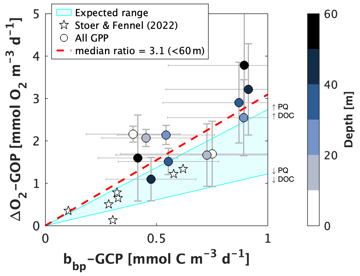
Figure 7A comparison of depth-resolved oxygen-based estimates of gross oxygen production (ΔO2-GOP) and particle backscattering-based estimates of gross carbon production (bbp-GCP) in waters shallower than 60 m. Data points represent values derived from co-located profiles in latitude bands or Longhurst provinces with enough profile measurements to obtain statistically consistent GPP estimates (Sect. 4.1.1). Error bars represent 1 standard error. Star markers represent GPP estimates from Stoer and Fennel (2023), which were obtained from co-located O2 and bbp profile measurements below the euphotic depth in the latitude range 30–60∘ S. GCP estimates were not converted to O2 equivalents, nor were they adjusted for potential PER. The light blue shading represents the expected range for the relationship between GOP and GCP, given a percent extracellular release (PER) range of 18 %–47 % (Moran et al., 2022) and photosynthetic quotient (PQ) range of 1–1.45 (Laws, 1991). The dashed line shows the median GOP : GCP ratio below 60 m.
Diurnal cycle GPP methods are based on the presumption that day–night variations in photosynthesis are the primary driver of diurnal variations in upper-ocean O2 or POC concentrations. Other than accounting for potential diurnal solubility impacts on O2 (through expressing O2 as its concentration anomaly, ΔO2), no attempts have been made to reconcile for additional diurnal variations in float estimates of O2 or POC that are not caused by photosynthesis. For O2, these include potential impacts due to air–sea exchange or vertical mixing, and for POC they are sinking, diel vertical migration and grazing, or PER. Yet, these processes vary throughout the day, and the extent to which they do changes seasonally and geographically. Diurnal variability in solar heating and wind forcing influence mixed layer dynamics on hourly or longer timescales, with impacts on air–sea gas exchange (Briggs et al., 2018) and near-surface vertical mixing (Price et al., 1986). Moreover, particle sinking, grazing, or DOC production have been implicated as a mechanism for decoupling O2- and POC-based PP estimates, particularly in high-productivity (e.g., diatom-dominated) regions (e.g., Rosengard et al., 2020). For example, regions of high POC sinking rates, grazing, or PER will decouple O2 and POC concentrations, leading to high O2 and low POC in upper-ocean waters, with implications for resulting GPP and CR estimates (White et al., 2017; Rosengard et al., 2020; Briggs et al., 2018). Similarly, day–night variations in grazing, resulting from diel vertical migrations, could amplify the nighttime decline in POC, thereby artificially inflating nighttime respiration estimates and decoupling O2- and POC-based GPP calculations. Independently or in combination, these processes likely imprint on the daily signals detected by BGC-Argo floats, whether by single assets or the composite of the array, and therefore constitute a source of uncertainty to the resulting GPP estimates.
The use of POC to estimate GPP also requires the assumption that gross community production is equal to autotrophic gross carbon production (White et al., 2017; Henderikx Freitas et al., 2022; Stoer and Fennel, 2023) and that daily cycles of non-algal particles are negligible. Often, however, this may not be the case. Moran et al. (2022) suggested that bacterial carbon production contributes a small, but highly variable, fraction to particulate PP equal to ∼ 13 ± 19 % (mean ± 1 standard deviation) or < 10 % of total PP if PER is ∼ 30 %. For the size range relevant to bbp, Martinez-Vicente et al. (2012) further suggested that the variability in bbp largely results from variability in phytoplankton between 2 and 20 µm in diameter, despite the majority of the bbp signal coming from highly abundant bacteria. Thus, if diurnal variability in bbp is mainly attributed to phytoplankton, then the bbp daily signal may still be a close proxy of GPP. Nonetheless, it is important to consider other potential sources of variability in bbp attributed to non-algal particles.
Variations in the bbp-to-POC relationship, both in space and in time, also contribute a key source of uncertainty in the POC-based GPP estimates. Several algorithms between bbp and POC exist, including the algorithm of Graff et al. (2015), which was derived using a latitudinally distributed dataset obtained from the Atlantic Meridional Transect and equatorial Pacific, as well as several regional ones (e.g., Loisel et al., 2011; Cetinić et al., 2012). We and Stoer and Fennel (2023) used a bbp-to-POC relationship based on a globally distributed dataset, which may not be appropriate for all ocean regions or depths (Bol et al., 2018). Moreover, diurnal variations in the bbp-to-POC relationship have been implicated in the uncertainties in bbp-POC-based GPP estimates in the Mediterranean and NW Atlantic (Briggs et al., 2018; Barbieux et al., 2022). Such variations may be attributed to changes in the phytoplankton carbon-to-bbp ratio (Poulin et al., 2018) or refractive index (Henderikx-Freitas et al., 2022), which will confound interpretations of particulate productivity. Beam-attenuation-based GCP estimates (cp-GCP), however, appear to be more reliable than those derived from bbp due to the dampened diurnal variability in the cp-to-POC relationship (Briggs et al., 2018; Barbieux et al., 2022). At this time, though, cp is not widely measured on BGC-Argo floats, and a far greater proportion of BGC-Argo floats already measure bbp.
Differences in sampling time and location, including offsets in the number and locations of O2 versus bbp profiles, will also contribute to uncertainty in GPP comparisons. This includes differences between the timing and locations of independent bottle samples (see markers in Fig. 1) and float profiles, as well as differences in the timing and location of float O2 and bbp profiles. For these reasons, it is not surprising that the relationship between ΔO2-GOP and bbp-GCP is less robust when considering the non-co-located float profiles (data not shown).
Finally, a critical number of profiles are needed to accurately estimate GPP from daily cycles of composite float profiles. As mentioned here and in previous studies (Johnson and Bif, 2021; Stoer and Fennel, 2023), a large number of floats are discarded from calculations because they do not sample all hours of the day evenly, presently reducing the number of profiles available for GPP calculations by ∼ 75 %. As a result, calculations are precluded in many regions or latitude bands, particularly those based on bbp, and the resulting values are likely less robust. In the N Atlantic Ocean, for example, many floats currently do not sample all hours of the day evenly (compare grey and coloured markers in Fig. 6a), preventing GPP calculations in a number of provinces in that region. For this method to be applied more broadly, floats need to cycle at all hours of the day. To achieve this, float manufacturers should ensure that the sampling protocols can be readily adjusted to the recommended profiling interval of 5.2 or 10.2 d by users via the float firmware. We discuss, in more detail, the minimum number of floats required for robust GPP calculations in the following section.
4.1.1 How many floats are required for consistent, annual GPP estimates?
Following Stoer and Fennel (2023), we performed a bootstrapping analysis to determine the number of O2 and bbp profiles required to obtain stable GOP or GCP estimates in different latitude bands. We performed the analysis in the 0–30 and 30–60∘ N/S latitude bands for O2-GOP and in the 0–30∘ N and 30–60∘ S regions for bbp-GCP. There are not enough bbp profiles currently available to perform the calculations outside of those regions. In each band, we calculated GPP from diurnal cycles constructed from a random subset of data, repeating calculations 1000 times for subset sizes between 500 and 12 000 profiles. As above, we did not sub-sample the profiles in time, such that our GPP estimates reflect an ensemble median value over the period of 2010–2022. From the resulting GPP estimates, we calculated the 0–100 m integrated quantities, and we derived a signal-to-noise ratio by dividing the standard deviation by the mean value. Unlike Stoer and Fennel (2023), who used a threshold ratio of one, we determined the minimum number of profiles required as the first subset size with a ratio less than 0.5.
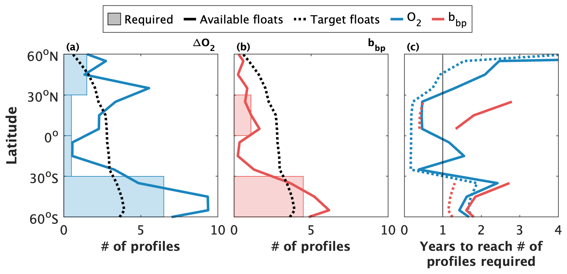
Figure 8Estimates of the number of profiles and time required to derive statistically consistent gross oxygen production (GOP) and gross carbon production (GCP) estimates at different latitude bands. The shaded regions in panels (a) and (b) represent the estimated number of profiles required for dissolved oxygen (O2) and particle backscattering (bbp), respectively. The minimum number of profiles required was calculated from a bootstrap analysis with a signal-to-noise threshold of 0.5. The solid lines represent the current number of profiles available for gross primary production calculations since 2010. The dashed lines represent estimates of the number of profiles obtained, per year, by a target Biogeochemical-Argo array of 1000 floats deployed ocean-wide proportionally with ocean surface area and profiling at 10.2 d intervals. Panel (c) shows an estimate of the time required to attain the minimum number of required profiles if the current active (January 2023; solid lines) and target (dashed lines) Biogeochemical-Argo array profiles at 10.2 d intervals. The time required was calculated as .
Our calculations suggest that between 500 (0–30∘ N) and 6500 (30–60∘ S) O2 profiles and between 1100 (0–30∘ N) and 4500 (30–60∘ S) bbp profiles are required to obtain robust annual GPP estimates from composite diurnal cycles (Fig. 8a and b). Previous estimates are somewhat lower: 20 or 50 O2 profiles per hour (480 or 1200 per day composite day) in tropical and high-latitude waters, respectively (Johnson and Bif, 2021), or 5000 O2 and 2000 bbp profiles south of 30∘ S (Stoer and Fennel, 2023). Regardless, these results imply that the horizontal and/or temporal resolution of GPP estimates derived from composite sampling is presently constrained by the number of floats available to attain the requisite number of profiles. While the total number of profiles collected by the BGC-Argo array since 2010 is sufficient to derive decadal O2-GOP, but not bbp-GCP, from composite daily cycles in most 10∘ latitude bands (compare solid lines and shaded region in Fig. 8a and b), more floats will be required to perform similar calculations in narrower latitude bands or biogeographic provinces. More floats are also necessary to yield GPP estimates with a better than ∼ 10-year temporal resolution.
Notably, our results indicate that the projected array of 1000 BGC-Argo floats (Roemmich et al., 2021; Biogeochemical-Argo Planning Group., 2016) should be sufficient to obtain annual, or better, GPP snapshots at most latitude bands. Assuming, for example, that the projected 1000-float array is deployed evenly in proportion to ocean surface area in each latitude band and that floats profile every 10.2 d, then the number of profiles obtained per year (dashed black lines in Fig. 8a and b) will be greater than the minimum threshold that we calculated in our bootstrapping analysis at many latitudes. Given these assumptions, there would be enough profiles to obtain sub-annual GPP estimates in regions equatorward of ∼ 30∘ N/S (dashed lines in Fig. 8c). More floats will be required towards the poles, although the achievable temporal resolution may still be less than 2 years in high-latitude Southern Ocean waters. This resolution cannot be achieved if floats are set to cycle at integer intervals (Sect. 3.2.1), but, in theory, if all floats are set to profile every 5.2 d (rather than 10.2 d), the duration to achieve the minimum profile threshold should be halved. Given the current BGC-Argo array, on the other hand, the best-available temporal resolution is typically greater than 1 year at all temperate or sub-polar latitude bands but may be less than 1 year in the tropics and subtropics (solid lines in Fig. 8c).
It is also noteworthy that our estimates of the minimum number of profiles required for consistent GPP estimates are based on the compilation of ΔO2 or bbp data obtained during all months of the year. Towards the poles, the amplitude and phase of diurnal productivity or biomass cycles differ between seasons, due, in part, to light constraints on productivity. The diurnal cycles constructed from a composite of measurements obtained throughout the year reflect somewhat conflicting signals from sampling at different times of year, making it more difficult to resolve a clear diurnal signal. As a result, it is likely that our threshold estimates represent an overestimate of the number of profiles required to obtain consistent seasonal GPP values in some regions. Unfortunately, however, there are an insufficient number of profiles presently available in a given season to repeat the analysis at higher temporal resolution.
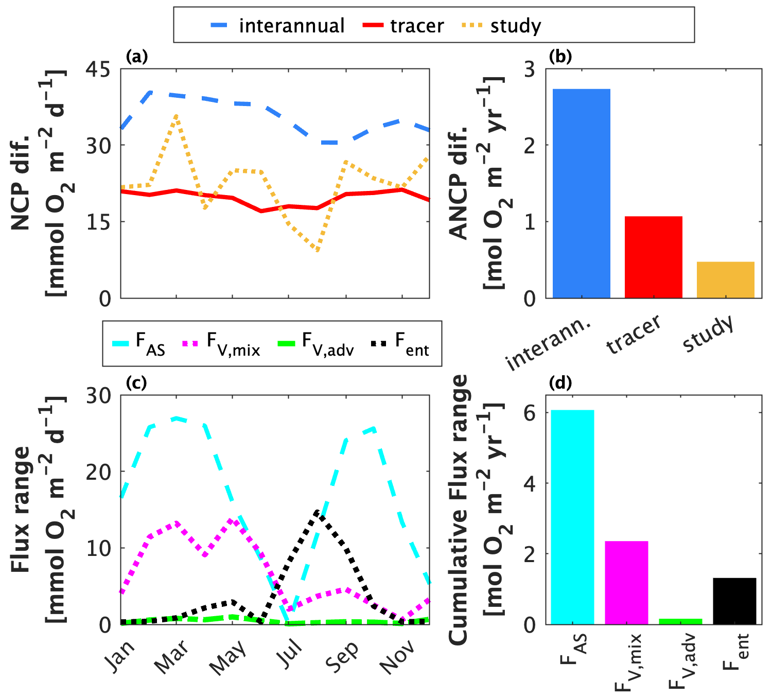
Figure 9Contributions to differences between float-based net community production (NCP) and annually integrated NCP estimates at Ocean Station Papa (OSP). Panels (a) and (b) show estimates of the contributions of different factors to differences in published mixed layer-integrated NCP and ANCP estimates from OSP. The blue line/bar represent differences due to real interannual NCP and ANCP variability; the red line/bar shows differences resulting from the choice of tracer; and the yellow line/bar represents differences between approach occurring between studies within the same year. Panels (c) and (d) represent estimates of the range of dissolved oxygen (O2) flux parameterizations across studies (Table 1). For each flux, values were calculated as the absolute range of estimates after applying the different parameterizations for each term (Table 1). FAS = air–sea flux via diffusion and bubbles; Fvmix = vertical transport flux via diapycnal mixing; Fvadv = vertical transport flux via advection; Fent = vertical transport flux via entrainment. Panel (d) shows the cumulative flux range over 1 year.
4.2 Constraints on NCP accuracy and coverage
The compiled OSP NCP time series (Fig. 5, Sect. 3.1) identified important differences between float-based NCP studies. Those differences can be attributed to one of the following: (1) real interannual NCP variability, (2) the tracer used to evaluate the NCP budget, or (3) the budget setup and parameterizations. We used the compiled OSP results to assess the potential role of each of those factors on time-resolved and annual-integrated NCP (Fig. 9a). To assess the natural interannual variability, we calculated the mean range of monthly NCP or annual ANCP across studies spanning multiple years (Plant et al., 2016; Yang et al., 2017). To determine the impact of tracer selection, we calculated the mean monthly range of values across studies that performed calculations using more than one tracer (Plant et al., 2016; Huang et al., 2022). To determine the role of the parameterization approach, we calculated the mean monthly range of values across all O2-based studies (Plant et al., 2016; Yang et al., 2017; Pelland et al., 2018) occurring within the same year.
Our analysis suggests that interannual NCP or ANCP variability is the largest contributor to differences between the float-based OSP NCP studies (Fig. 8a and b). Between-tracer and between-approach differences are similar in magnitude for time-resolved NCP estimates, but between-approach differences are smallest across ANCP estimates. Interannual differences are largest in the early spring, which may reflect year-to-year differences in the onset of the spring bloom or the end of wintertime heterotrophy. There are no apparent seasonal patterns in the between-tracer or between-approach differences, although between-tracer differences are somewhat smaller during the summer.
As described in Sect. 2.1, between-tracer differences reflect how the tracers target different components of the carbon pool and system (Huang et al., 2022). Calculations based on O2 and reflect particulate and dissolved organic C cycling, while POC-based calculations only reflect the fraction of suspended POC. DIC or TA budgets, meanwhile, are influenced by organic and inorganic C cycling. Differences between O2- and -based estimates, moreover, are sensitive to the relative importance of new production (based on ) versus recycled production (based on ), and, to a lesser degree, denitrification and N2 fixation. For example, under fully recycled production, O2-based NCP estimates would reflect O2 production during photosynthesis, while concentrations would be unchanged. As a result, O2-based estimates would exceed -based values. Similarly, denitrification and N2 fixation would affect the decoupling between -based estimates and estimates derived using other tracers if the consumption/production of during those processes is unaccounted for in the NCP budget calculations. Indeed, if the source of N2 fixation is unaccounted for, the resulting NCP estimated will be biased low. This bias is particularly problematic for oligotrophic waters (e.g., Huang et al., 2023).
It is possible to partition some of the processes and carbon pools by performing simultaneous NCP calculations using multiple tracers (Huang et al. 2022), but in the absence of such calculations, it is important to consider how the tracer selection influences the interpretation of NCP results. In addition, the between-tracer differences also somewhat reflect the importance of different flux parameterizations used in the budget calculations. For example, calculations based on O2 require estimates of the air–sea flux term, while those based on do not. As a result, those estimates based on may be perceived to be somewhat more accurate, due to the large air–sea flux uncertainties (e.g., Bender et al., 2011; Emerson and Bushinsky, 2016).
The between-method differences reflect differences in the flux parameterizations and NCP budget setup between studies, which are summarized in Sect. 2.2 and Table 1. We examined the contributions of different fluxes to the overall differences between approaches by calculating the range of physical fluxes (air–sea, vertical mixing, entrainment, and vertical advection) applied in the different studies at OSP (Fig. 9c and d). To estimate the range of air–sea fluxes represented in the OSP studies, we calculated monthly average surface water O2 and O2,eq using BGC-Argo observations collected from OSP between 2008 and 2020. We then applied the different O2 air–sea flux parameterization schemes (Table 1) and calculated the resulting range of values. Similarly, we used BGC-Argo observations to the range of vertical fluxes by determining the average monthly subsurface vertical O2 gradient ( in Eq. 7.6) and concentration difference (Δ[T]Z in Eqs. 7.7 and 7.8), and we multiplied those values by the different eddy diffusivity (κZ), vertical advection (u) and entrainment () values applied in the OSP studies. Our analyses indicate that the air–sea flux and vertical mixing fluxes are the most variable across studies, contributing large uncertainty in time-resolved and annually integrated NCP (Fig. 9c and d). Previous work has similarly identified air–sea flux and eddy diffusive mixing as two of the most important sources of uncertainty in their ANCP calculations, up to ∼ 0.7 and 0.3 , respectively (Bushinsky and Emerson, 2015; Plant et al., 2016; Yang et al., 2017). Moreover, Plant et al. (2016) estimated an ANCP range of nearly 2 when applying different air–sea flux parameterizations to their calculations, and a range of ∼ 1 was calculated between ANCP estimates derived using regionally tuned versions of the Liang et al. (2013) air–sea flux model and an un-tuned version (Plant et al., 2016; Yang et al., 2017).
Another important constraint on the accuracy of float-based NCP estimates is the measurement accuracy of the BGC variable. A ± 1 % error in O2, for example, can contribute between 0.3 and 2 of uncertainty to ANCP estimates (Bushinsky and Emerson, 2015; Yang et al., 2017; Huang et al., 2018), comparable in magnitude to uncertainties resulting from air–sea flux and diffusive mixing. Plant et al. (2016) also found that a ± 1 % O2 error results in ∼ ± 10 error in time-resolved NCP and, in some cases, causes a shift in the apparent upper-ocean metabolic state (i.e., a shift between net heterotrophy and net autotrophy), particularly during the transition seasons. Moreover, budget calculations may be subject to considerable uncertainty in oligotrophic regions when the concentration is close to the sensor's signal-to-noise ratio. In some cases, erroneous float data should preclude NCP calculations altogether (Plant et al., 2016), and, in general, NCP calculations cannot be performed reliably on unadjusted BGC-Argo data. Another potential source of NCP uncertainty resulting from the air–sea flux parameterization is the impact of sea-level pressure on gas solubility. In the diffusive air–sea flux equation described by Eq. 7.3, the term [T(t,0)]eq refers to the gas saturation concentration at ambient sea level pressure (PSLP), which can be calculated from empirical solubility algorithms (e.g., Garcia and Gordon, 1992). These algorithms describe the saturation concentration at 1 atm, yet the saturation concentration in situ is impacted by PSLP, such that , where P is pressure and is the pressure due to water vapour. In temperate and high-latitude regions where PSLP is typically lower than 1 atm, neglecting to account for this effect may lead to an overestimate in the importance of the diffusive air–sea flux term and a corresponding underestimate in NCP. Such impacts will only be relevant to gas-based budget calculations and will be most important for those based on O2. Future work should thus endeavour to address this important detail.
Similarly, it is important to note that budget-based NCP calculations assume that the float follows the same water mass over the duration of the calculation period. However, floats may often transition into adjacent water masses, making the interpretation of observed tracer changes somewhat challenging. The resulting uncertainty in NCP calculations may be important, but it is difficult to constrain. In some cases, if floats are judged to transition between different water masses (e.g., by assessing water mass temperature and salinity properties), NCP calculations may be precluded altogether.
It is noteworthy that our analysis does not reveal which methods are most accurate. Rather, our analyses were intended to identify sources of variability across NCP studies. Moreover, our case study focused exclusively on OSP, which is well studied with respect to upper-ocean mixing fluxes (Cronin et al., 2015), air–sea exchange (e.g., Emerson and Bushinsky, 2016; Emerson et al., 2019; Steiner et al., 2007; Vagle et al., 2010), and NCP. That many other ocean regions are not so well characterized may ultimately limit the current capacity to derive accurate float-based NCP estimates. Future work should thus endeavour to better understand the relative importance and magnitude of the physical fluxes in a variety of ocean regions. In doing so, efforts to tune air–sea flux parameterizations for regional conditions (e.g., Plant et al., 2016; Yang et al., 2017; Emerson et al., 2019; Haskell et al., 2020) or to identify the most accurate parameterization in different basins (e.g., Atamanchuk et al., 2020) should be undertaken. Approaches like the one employed by Pelland et al. (2018) to evaluate the physical mixing terms from temperature or salinity budget calculations based on in situ profiler data should also be made alongside corresponding NCP budget calculations.
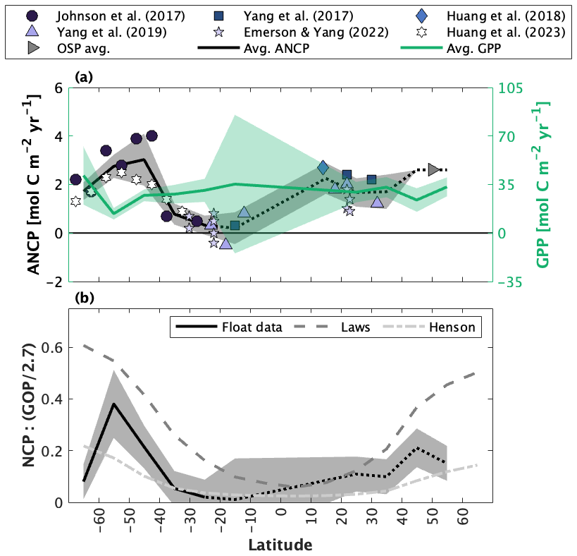
Figure 10The latitudinal distribution of float-derived annual-average gross primary production (GPP), annually integrated net primary production (ANCP), and the export ratio (equal to GPP divided by ANCP). GPP estimates in (a) are gross oxygen productivity estimates from oxygen measurements (ΔO2-GOP) integrated within the euphotic zone and converted to carbon equivalents using a photosynthetic quotient value of 1.4. ANCP values are from various data sources, as indicated in the figure legend or from the compilation of Ocean Station Papa data in Sect. 3.1 (Fig. 5). Note that values from Johnson et al. (2017b) represent NCP calculated from drawdown over the austral productive period; we did not perform any corrections to adjust those values to represent annually integrated NCP. The data from Huang et al. (2023) represent the average of and DIC-based ANCP estimates. The black line and shading represent average ± 1 standard deviation values in 10∘ latitude bands. In (b), a float-based estimate of the export ratio was derived by dividing average float-based ANCP by float-based net primary productivity (NPP), using an GOP-to-NPP ratio of 2.7, as in Johnson and Bif (2021) and Stoer and Fennel (2023). Independent estimates of the export ratio from Laws et al. (2011) and Henson et al. (2012) are also shown. The dotted black lines north of 30∘ S indicate poorer latitudinal representation of float-based ANCP, and therefore lower confidence in the derived export ratio.
The BGC-Argo fleet offers global observations of real-time ocean biogeochemistry, enabling widespread PP measurements that are independent of, yet complementary to, satellite and ship-based approaches. However, compared with PP methods that rely on traditional sampling infrastructure, float-based methods confer significant advantages in detecting PP. Float-based methods, for example, provide simultaneous horizontal, vertical, and temporal PP coverage, presenting the opportunity to fill key gaps in the existing PP data record (Fig. 1). Moreover, while recent efforts towards FAIR data principles (Tanhua et al., 2019) have improved the availability of ship and bottle data, resulting PP datasets remain generally inaccessible (e.g., spread over disconnected repositories) and non-standardized (e.g., datasets are often published individually with a single paper/project and therefore follow no archiving or metadata guidelines). Float data, in contrast, are generally made available within 24 h of collection, are publicly available, and are archived following agreed-upon guidelines (Bittig et al., 2019), enabling cost-effective, open-source PP calculations that can be independently verified and applied by the entire science community, including those without the resources to perform traditional PP methods. Lastly, float-based methods facilitate enhanced detection of the biological response to unpredictable or episodic events like wildfires, volcanic eruptions, or bloom periods, which often cannot be sufficiently characterized using traditional in situ datasets (Tang et al., 2021).
As float-based techniques mature, the BGC-Argo fleet can be used to extend our current understanding of the marine GPP, NPP, NCP, and C export, particularly at scales that have so far only been achieved through satellite-based algorithms (e.g., Behrenfeld and Falkowski, 1997; Laws et al., 2011). For example, by compiling the data discussed and derived in this paper, we can calculate independent, global estimates of the carbon export ratio (equivalent to ANCP divided by NPP, where NPP is derived from float-GOP; Fig. 10). Notwithstanding the regional and temporal biases in current float-based PP estimates, these C export ratio estimates are consistent with the commonly used satellite models of Laws et al. (2011) and Henson et al. (2012). Simultaneous estimates of GPP, NCP, and C export are rarely made, let alone comparisons between them. Thus, the export ratio we derived here could be an important tool for improving our understanding of the ocean carbon cycle. Moving forward, the extent to which float-based PP calculations can be applied will depend, to a large degree, on the availability of float data (Sect. 4.1.1) and our capacity to better constrain key sources of uncertainty in biogeochemical budget interpretations (Sects. 4.1 and 4.2). Indeed, to increase the availability of float-based PP data, expansion of the Argo fleet should be prioritized, particularly in undersampled ocean regions. Floats will need to be deployed with sampling intervals set to 5.2 or 10.2 d (rather than 5.0 or 10.0 d) to properly detect diurnal variability. Finally, fully exploiting floats for PP measurements will rely on the open availability of PP datasets, including processed data and relevant software.
Ultimately, continued efforts towards expanding and refining float-based PP datasets will reduce uncertainties in the present methods, yielding widespread in situ PP estimates in most ocean basins. As uncertainties are further constrained, the resulting estimates will convey significant tangential benefits, like the ability to improve numerical model predictions through data assimilation (e.g., B. Wang et al., 2020) and to train and/or validate satellite PP algorithms, as has been done previously using ship data (e.g., Li and Cassar, 2016; Huang et al., 2021). Given the on-going expansion of the BGC-Argo array and the continued generation of significant amounts of biogeochemical data, the resulting products can be continually retrained and evaluated using new methods and datasets. Achieving these milestones will enable unprecedented in situ classification of the response and variability of marine PP to various environmental perturbations over a range of spatial and temporal scales.
Data handling and calculations for the OSP NCP case study
We compiled NCP and ANCP data from six published float/glider studies at Ocean Station Papa (OSP) in the subarctic NE Pacific (Table A1). Time-explicit NCP and ANCP values were obtained from Plant et al. (2016), Yang et al. (2017), Pelland et al. (2018), Haskell et al. (2020), and Huang et al. (2022). We also obtained an estimate of ANCP from Bushinsky and Emerson (2015). Yang et al. (2017) and Haskell et al. (2020) provided NCP data that were integrated to the depth of the annual maximum mixed layer (ML), while Plant et al. (2016) and Pelland et al. (2018) provided depth-resolved estimates. Data from Huang et al. (2022) were integrated to 56 m. We present NCP and ANCP values integrated to the annual maximum mixed layer depth (MLD), scaling values from Huang et al. (2022) to maximum MLD (i.e., NCP estimates from Huang et al. (2022) were scaled by dividing values from that publication by 56 m and then multiplying by an annual maximum MLD of 120 m for OSP). We appreciate that this approach may result in an overestimate in maximum MLD-integrated NCP values from Huang et al. (2022) as it assumes constant NCP between 56 m and the maximum MLD, which is likely not the case.
We also obtained NCP estimates from ship-board sampling, moorings, and satellites, collected over the past 2 decades (Table A1). We obtained two satellite-based NCP estimates: one from a global machine learning algorithm (Li and Cassar, 2016) and the other derived as the product of satellite-NPP (average of the VGPM and CbPM models; Behrenfeld and Falkowski, 1997; Westberry et al., 2008) and a commonly used global export-ratio algorithm (e-ratio; Laws et al., 2011) (i.e., NCP = NPP × e-ratio). The ship and mooring estimates represent NCP values integrated in the seasonal ML, while satellite-based estimates detect approximately 1 optical depth below the surface. Accordingly, we scaled all independent NCP estimates to the annual average maximum MLD at OSP, as described above, using MLD estimates obtained from the Argo Mixed Layers climatology (Holte et al., 2017).
We calculated ANCP as the sum of annual maximum MLD-integrated values from January through to December for each full year of data. We determined ship-based ANCP by integrating average monthly ML-integrated NCP values over a 12-month cycle, after linearly interpolating values between months without data. All units were converted to O2 equivalents using a PQ value of 1.4 and an O2: ratio of 150:16.
Data handling and calculations for the global GPP case study
Following Stoer and Fennel (2023), we compiled all available BGC-Argo O2 and bbp,700 data collected between January 2010 and December 2022, selecting only the high-quality (Argo quality flags 1 and 2 representing “good”, and “probably good”), “adjusted” (flag 5), and “estimated” (flag 8) O2 data and high-quality bbp data. The bbp profiles were de-spiked using a five-point running minimum filter followed by a five-point running maximum filter. Profile measurements were then binned into 10 m intervals from 0 to 200 m depth. We applied linear interpolation between up to two data points when data were missing. We calculated ΔO2 (mmol m−3) using the corresponding float hydrographic data (Garcia and Gordon, 1993, 1992) and POC (mmol m−3) following the bbp-to-POC algorithm of Graff et al. (2015), after converting bbp,700 to bbp,470 using a power-law relationship with a slope of 0.78 (Boss and Haëntjens, 2016; Boss et al., 2013).
Treating O2 and bbp separately, we excluded a selection of floats with oceanographically inconsistent data or unrealistic O2 and bbp values (see lists in Johnson and Bif, 2021, and Stoer and Fennel, 2023). We discarded any floats that did not sample at least 21 unique hours of the day evenly over their life cycles. Profiles were subdivided into different spatial groups, representing 10∘ latitudinal bands (70∘ S to 70∘ N) or Longhurst biogeographical provinces. We constructed a composite diurnal curve in each spatial subset by calculating the median ΔO2 or bbp-POC value at each hour of the day.
We performed two sets of GPP calculations only when at least 21 h of the day were represented in each subset: (1) using all available ΔO2 and bbp-POC profiles, treating O2 and bbp independently, and (2) using co-located data obtained from floats containing both O2 and bbp sensors. GOP and GCP were estimated by fitting the sinusoidal GPP-vs-light function to the resulting diurnal curves. We did not consider the influence of fluxes due to air–sea exchange, vertical mixing, POC sinking, or grazing on our calculated GPP estimates. We used each data subset's average location and midpoint date to determine the daily light cycle and sunrise/sunset times. We accounted for DOC production by scaling bbp-GPP estimates by a percent extracellular release (PER) value of 0.33, calculated from the global meta-analysis of Moran et al. (2022), and converted GCP values (units mmol C) to O2 equivalents using a photosynthetic quotient of 1.4 (Laws, 1991) (i.e., . Finally, we discarded unrealistic GOP and GCP rates by removing values exceeding 3 standard deviations of the mean of a climatological GOP dataset (references listed in Table A1 of the Appendix). We did not specifically discard negative values, following the recommendation by Barone et al. (2019), but recognize those estimates as representing undetectably low GPP.
Table A1List of data sources and archived primary productivity (PP) datasets referenced in the paper.
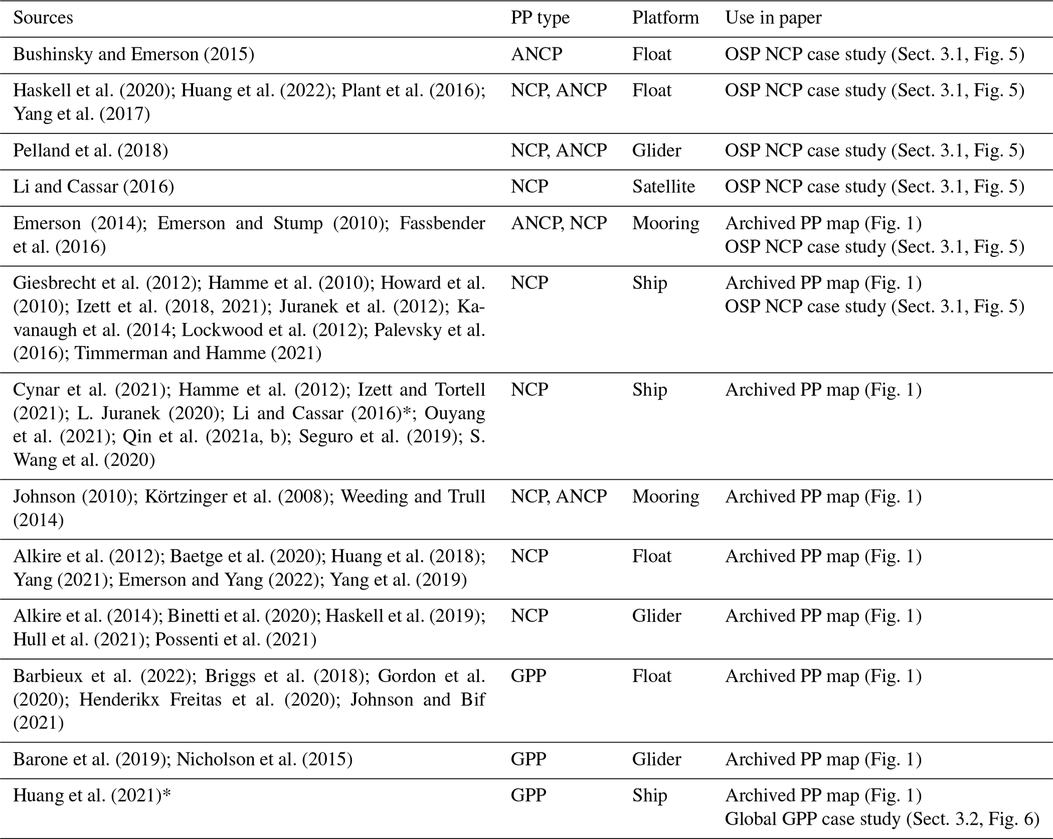
OSP = Ocean Station Papa; GPP = gross primary productivity; NCP = net community production; ANCP = annually integrated NCP; * Data compiled by Li and Cassar (2016) and Huang et al. (2021).
Table A2Summary of published float-based GPP and NCP studies. [g] denotes glider-based studies.
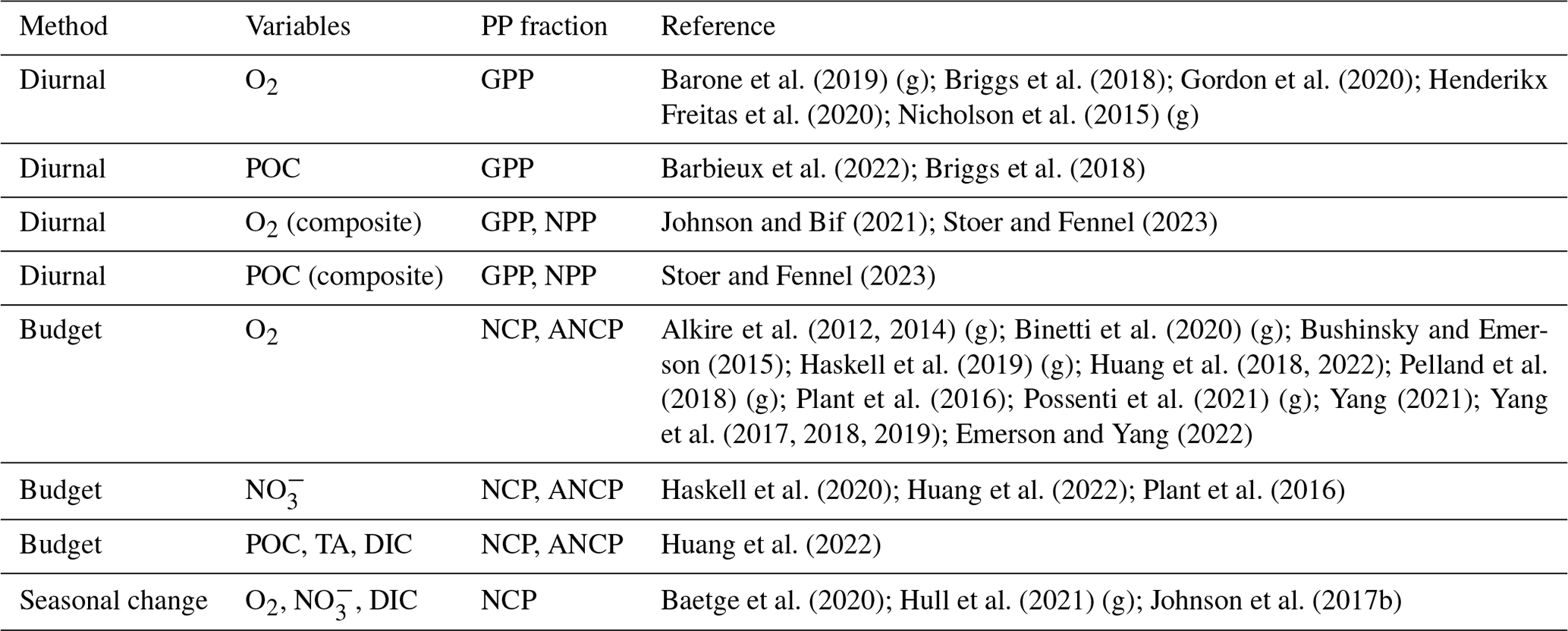
O2 = dissolved oxygen; POC = particulate organic carbon; = nitrate; DIC = dissolved inorganic carbon; TA = total alkalinity; GPP = gross primary productivity; NCP = net community production; ANCP = annually integrated NCP; * Data compiled by Li and Cassar (2016) and Huang et al. (2021).
Table A3Variations in budget terms used in float- and glider-based NCP calculations.
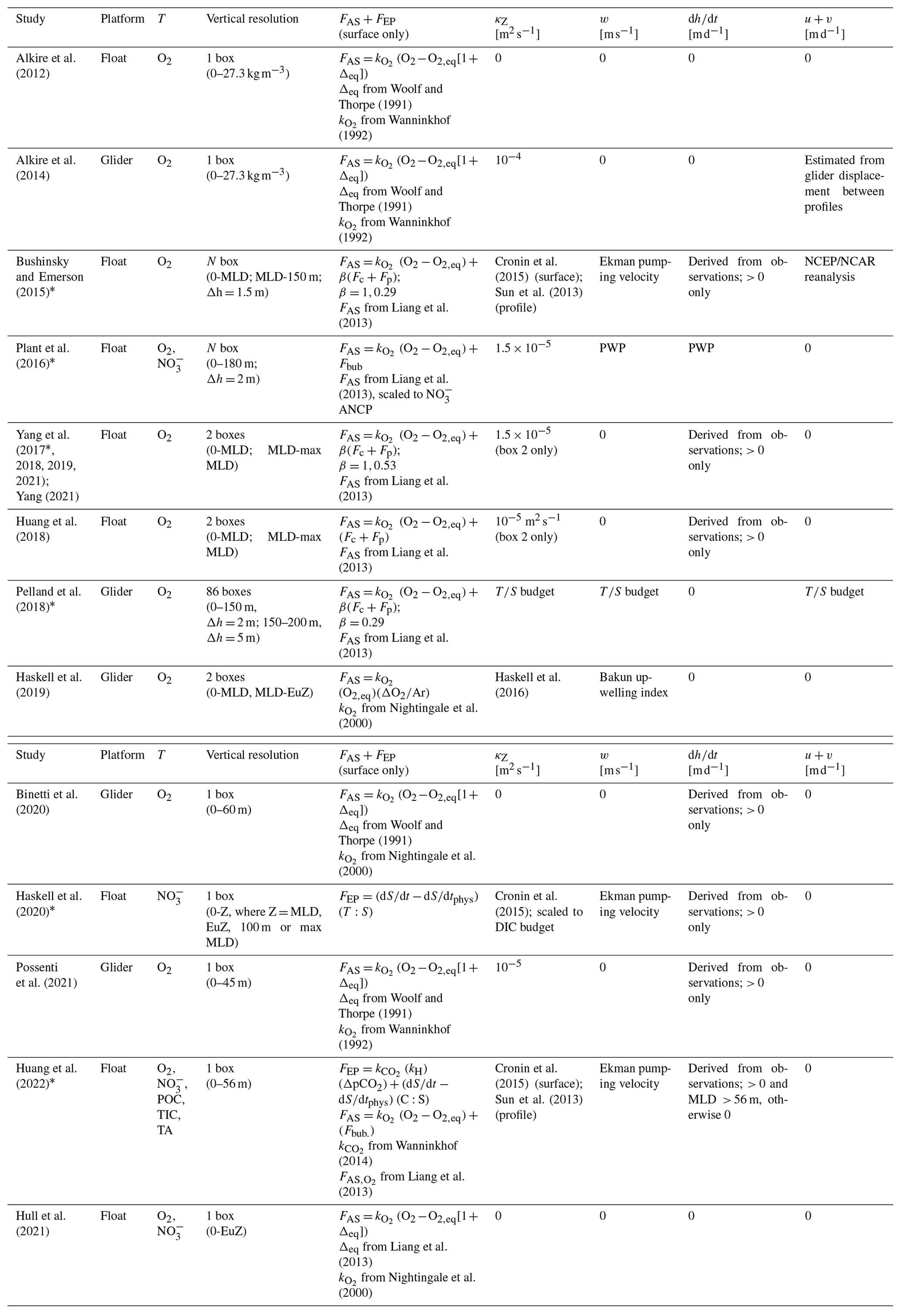
∗ = Studies at OSP; O2 = oxygen concentration (mol m−3); POC = particulate organic carbon concentration (mol m−3); = nitrate concentration (mol m−3); DIC = dissolved inorganic carbon concentration (mol m−3); TA = total alkalinity (mol m−3); MLD = mixed layer depth; FAS = air–sea gas exchange (); Fbub = air–sea bubble flux (); FEP = evaporation or precipitation (); and = air–sea gas transfer coefficient for O2 and CO2; κZ = eddy diffusivity coefficient [m2 d−1]; w = vertical advection velocity [m d−1]; = change in layer depth [m d−1]; u + v = horizontal advection velocities [m d−1]; Δh = box vertical displacement ( in Eq. 7); β = bubble-mediated transfer scaling coefficient [unitless]; PWP = Price–Weller–Pinkel mixed layer model (Price et al., 1986); C:S = observed DIC : salinity ratio [mol C:S]. “Surface” refers to values derived in the mixed layer only, while “profile” is for values derived over the full water column.
Table A4A comparison of algorithms for estimating particulate organic carbon (POC, mg m−3) from the beam attenuation coefficient (cp, m−1) and particle backscattering coefficient (bbp, m−1). The wavelength of the cp and bb measurements is indicated with a subscripted number (e.g., cp,660 indicates measurements at 660 nm). This table is not a complete list; the equations were selected to illustrate variability in POC relationships.
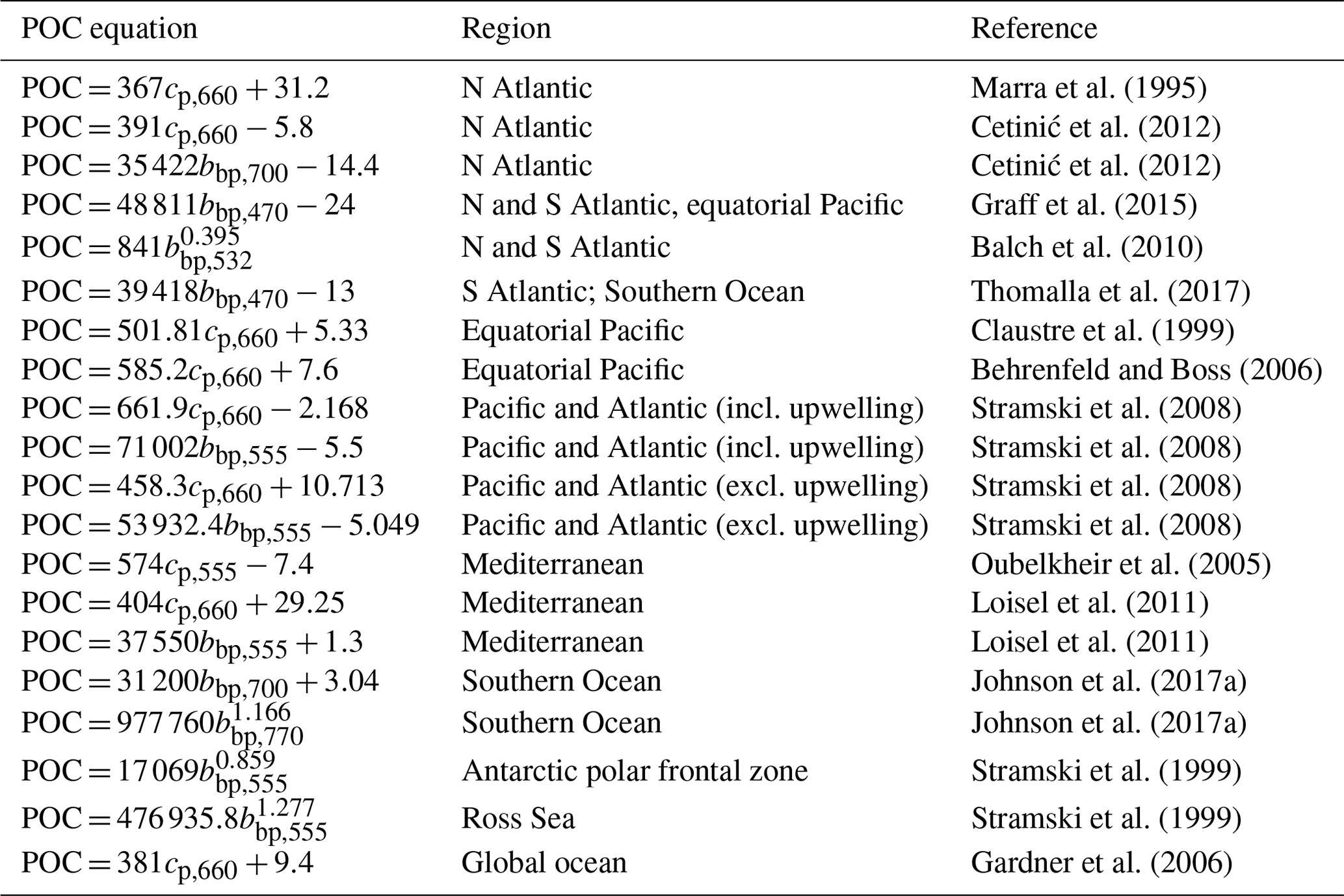
The GPP data in our global case study analysis were derived by modifying the code provided by Stoer and Fennel (2022). The code was only modified to perform GPP calculations in the geographic regions (10∘ latitude bands and Longhurst biogeographic provinces) described in the main text. Shapefiles for the Longhurst biogeographic province boundaries are available from Flanders Marine Institute (2009). NCP data from our OSP case study analysis is available from Izett et al. (2023). Additional GPP and NCP data included in this paper were compiled from the publications listed in Table A1 of Appendix A. BGC-Argo data were collected and made freely available by the International Argo Program and the national programmes that contribute to it (Argo, 2023). The International Argo Program is part of the Global Ocean Observing System. Float data are available from the Argo Global Data Assembly Centres in Brest, France (ftp://ftp.ifremer.fr/ifremer/argo, last access: 24 February 2023), and Monterey, USA (ftp://usgodae.org/pub/outgoing/argo, last access: 24 February 2023).
All authors contributed to the planning and preparation of the manuscript. RWI wrote the manuscript, with significant contributions and feedback from all authors. ACS performed the global GPP calculations. RWI compiled the OSP NCP data and performed all analyses on the GPP and NCP data.
The contact author has declared that none of the authors has any competing interests.
Publisher's note: Copernicus Publications remains neutral with regard to jurisdictional claims made in the text, published maps, institutional affiliations, or any other geographical representation in this paper. While Copernicus Publications makes every effort to include appropriate place names, the final responsibility lies with the authors.
We would like to thank the BGC-Argo community for supporting the float array through funding acquisitions, deployments, and data management, as well as for making the resulting data freely available. We also thank many colleagues for making their processed data available for analysis in this paper. In particular, we thank Andrea Fassbender, William Haskell, Yibin Huang, Noel Pelland, Joshua Plant and Bo Yang for their assistance. This work was supported by the Ocean Frontier Institute (OFI) and Canada First Research Excellence Fund (CFREF) through an International Postdoctoral Fellowship to Robert W. Izett. Katja Fennel received support from the Natural Sciences and Engineering Research Council of Canada (NSERC) through a Discovery Grant (RGPIN-2014-03938). Adam C. Stoer was supported by a Nova Scotia Graduate Student scholarship and by NSERC through a Canada Graduate Scholarship. David P. Nicholson was supported by the National Science Foundation's (NSF) Global Ocean Biogeochemistry Array (GO-BGC) project under the NSF Award 1946578 with operational support from NSF Award 2110258, as well as support from NSF OCE no. 2023080.
This research has been supported by the Ocean Frontier Institute (grant no. International Postdoctoral Fellowship), the Natural Sciences and Engineering Research Council of Canada (grant nos. RGPIN-2014-03938 and Canada Graduate Scholarships – Masters), and the National Science Foundation (grant nos. 1946578, 2110258, and 2023080).
This paper was edited by Koji Suzuki and reviewed by Yibin Huang and two anonymous referees.
Ainsworth, C. H., Samhouri, J. F., Busch, D. S., Cheung, W. W. L., Dunne, J., and Okey, T. A.: Potential impacts of climate change on Northeast Pacific marine foodwebs and fisheries, ICES J. Mar. Sci., 68, 1217–1229, https://doi.org/10.1093/icesjms/fsr043, 2011.
Alkire, M. B., D'Asaro, E., Lee, C., Jane Perry, M., Gray, A., Cetinić, I., Briggs, N., Rehm, E., Kallin, E., Kaiser, J., and González-Posada, A.: Estimates of net community production and export using high-resolution, Lagrangian measurements of O2, , and POC through the evolution of a spring diatom bloom in the North Atlantic, Deep Sea Res., 64, 157–174, https://doi.org/10.1016/j.dsr.2012.01.012, 2012.
Alkire, M. B., Lee, C., D'Asaro, E., Perry, M. J., Briggs, N., Cetinić, I., and Gray, A.: Net community production and export from Seaglider measurements in the North Atlantic after the spring bloom, J. Geophys. Res.-Oceans, 119, 6121–6139, https://doi.org/10.1002/2014JC010105, 2014.
Argo: Argo float data and metadata from Global Data Assembly Centre (Argo GDAC), SEANOE [data set], https://doi.org/10.17882/42182, 2023.
Arteaga, L. A., Pahlow, M., Bushinsky, S. M., and Sarmiento, J. L.: Nutrient Controls on Export Production in the Southern Ocean, Global Biogeochem. Cy., 33, 1–15, https://doi.org/10.1029/2019gb006236, 2019.
Arteaga, L. A., Behrenfeld, M. J., Boss, E., and Westberry, T. K.: Vertical Structure in Phytoplankton Growth and Productivity Inferred From Biogeochemical-Argo Floats and the Carbon-Based Productivity Model, Global Biogeochem. Cy., 36, e2022GB007389, https://doi.org/10.1029/2022GB007389, 2022.
Atamanchuk, D., Koelling, J., Send, U., and Wallace, D. W. R.: Rapid transfer of oxygen to the deep ocean mediated by bubbles, Nat. Geosci., 13, 232–237, https://doi.org/10.1038/s41561-020-0532-2, 2020.
Baetge, N., Graff, J. R., Behrenfeld, M. J., and Carlson, C. A.: Net Community Production, Dissolved Organic Carbon Accumulation, and Vertical Export in the Western North Atlantic, Front. Mar. Sci., 7, 1–16, https://doi.org/10.3389/fmars.2020.00227, 2020.
Balch, W. M., Bowler, B. C., Drapeau, D. T., Poulton, A. J., and Holligan, P. M.: Biominerals and the vertical flux of particulate organic carbon from the surface ocean, Geophys. Res. Lett., 37, L22605, https://doi.org/10.1029/2010GL044640, 2010.
Baines, S. B. and Pace, M. L.: The production of dissolved organic matter by phytoplankton and its importance to bacteria: Patterns across marine and freshwater systems, Limnol. Oceanogr., 36, 1078–1090, https://doi.org/10.4319/lo.1991.36.6.1078, 1991.
Barbieux, M., Uitz, J., Mignot, A., Roesler, C., Claustre, H., Gentili, B., Taillandier, V., D'Ortenzio, F., Loisel, H., Poteau, A., Leymarie, E., Penkerc'h, C., Schmechtig, C., and Bricaud, A.: Biological production in two contrasted regions of the Mediterranean Sea during the oligotrophic period: an estimate based on the diel cycle of optical properties measured by BioGeoChemical-Argo profiling floats, Biogeosciences, 19, 1165–1194, https://doi.org/10.5194/bg-19-1165-2022, 2022.
Barone, B., Nicholson, D., Ferrón, S., Firing, E., and Karl, D.: The estimation of gross oxygen production and community respiration from autonomous time-series measurements in the oligotrophic ocean, Limnol. Oceanogr.-Meth., 17, 650–664, https://doi.org/10.1002/lom3.10340, 2019.
Behrenfeld, M. J. and Boss, E.: Beam attenuation and chlorophyll concentration as alternative optical indices of phytoplankton biomass, J. Mar. Res., 64, 431–451, 2006.
Behrenfeld, M. J. and Falkowski, P. G.: Photosynthetic rates derived from satellite-based chlorophyll concentration, Limnol. Oceanogr., 42, 1–20, https://doi.org/10.4319/lo.1997.42.1.0001, 1997.
Bender, M., Grande, K., Johnson, K., Marra, J., Williams, P. J. L. B., Sieburth, J., Pilson, M., Langdon, C., Hitchcock, G., Orchardo, J., Hunt, C., Donaghay, P., and Heinemann, K.: A comparison of four methods for determining planktonic community production, Limnol. Oceanogr., 32, 1085–1098, https://doi.org/10.4319/lo.1987.32.5.1085, 1987.
Bender, M. L., Kinter, S., Cassar, N., and Wanninkhof, R.: Evaluating gas transfer velocity parameterizations using upper ocean radon distributions, J. Geophys. Res., 116, 1–11, https://doi.org/10.1029/2009JC005805, 2011.
Bif, M. B. and Hansell, D. A.: Seasonality of Dissolved Organic Carbon in the Upper Northeast Pacific Ocean, Global Biogeochem. Cy., 33, 526–539, https://doi.org/10.1029/2018GB006152, 2019.
Binetti, U., Kaiser, J., Damerell, G. M., Rumyantseva, A., Martin, A. P., Henson, S., and Heywood, K. J.: Net community oxygen production derived from Seaglider deployments at the Porcupine Abyssal Plain site (PAP; northeast Atlantic) in 2012–13, Prog. Oceanogr., 183, 102293, https://doi.org/10.1016/j.pocean.2020.102293, 2020.
Biogeochemical-Argo Planning Group: The Scientific rationale, design and Implementation Plan for a Biogeochemical-Argo float array, 2016.
Bittig, H. C., Steinhoff, T., Claustre, H., Fiedler, B., Williams, N. L., Sauzède, R., Körtzinger, A., and Gattuso, J.-P.: An Alternative to Static Climatologies: Robust Estimation of Open Ocean CO2 Variables and Nutrient Concentrations From T, S, and O2 Data Using Bayesian Neural Networks, Front. Mar. Sci., 5, 328, https://doi.org/10.3389/fmars.2018.00328, 2018.
Bittig, H. C., Maurer, T. L., Plant, J. N., Schmechtig, C., Wong, A. P. S., Claustre, H., Trull, T. W., Udaya Bhaskar, T. V. S., Boss, E., Dall'Olmo, G., Organelli, E., Poteau, A., Johnson, K. S., Hanstein, C., Leymarie, E., Le Reste, S., Riser, S. C., Rupan, A. R., Taillandier, V., Thierry, V., and Xing, X.: A BGC-Argo Guide: Planning, Deployment, Data Handling and Usage, Front. Mar. Sci., 6, https://doi.org/10.3389/fmars.2019.00502, 2019.
Bol, R., Henson, S. A., Rumyantseva, A., and Briggs, N.: High-Frequency Variability of Small-Particle Carbon Export Flux in the Northeast Atlantic, Global Biogeochem. Cy., 32, 1803–1814, https://doi.org/10.1029/2018GB005963, 2018.
Bopp, L., Resplandy, L., Orr, J. C., Doney, S. C., Dunne, J. P., Gehlen, M., Halloran, P., Heinze, C., Ilyina, T., Séférian, R., Tjiputra, J., and Vichi, M.: Multiple stressors of ocean ecosystems in the 21st century: projections with CMIP5 models, Biogeosciences, 10, 6225–6245, https://doi.org/10.5194/bg-10-6225-2013, 2013.
Boss, E., Picheral, M., Leeuw, T., Chase, A., Karsenti, E., Gorsky, G., Taylor, L., Slade, W., Ras, J., and Claustre, H.: The characteristics of particulate absorption, scattering and attenuation coefficients in the surface ocean; Contribution of the Tara Oceans expedition, Methods in Oceanography, 7, 52–62, https://doi.org/10.1016/j.mio.2013.11.002, 2013.
Boss, E. B. and Haëntjens, N.: Primer regarding measurements of chlorophyll fluorescence and the backscattering coefficient with WETLabs FLBB on profiling floats, SOCCOM, Princeton University, https://doi.org/10.25607/OBP-50, 2016.
Boyd, P. W., Trull, T. W.: Understanding the export of biogenic particles in oceanic waters: is there consensus?, Prog. Oceanogr., 72, 276–312, https://doi.org/10.1016/j.pocean.2006.10.007, 2007.
Briggs, N., Guðmundsson, K., Cetinić, I., D'Asaro, E., Rehm, E., Lee, C., and Perry, M. J.: A multi-method autonomous assessment of primary productivity and export efficiency in the springtime North Atlantic, Biogeosciences, 15, 4515–4532, https://doi.org/10.5194/bg-15-4515-2018, 2018.
Burt, W. J., Westberry, T. K., Behrenfeld, M. J., Zeng, C., Izett, R. W., and Tortell, P. D.: Carbon: Chlorophyll ratios and net primary productivity of Subarctic Pacific surface waters derived from autonomous shipboard sensors, Global Biogeochem. Cy., 32, 267–288, https://doi.org/10.1002/2017GB005783, 2018.
Bushinsky, S. M. and Emerson, S.: Marine biological production from in situ oxygen measurements on a profiling float in the subarctic Pacific Ocean, Global Biogeochem. Cy., 29, 2050–2060, https://doi.org/10.1002/2015GB005251, 2015.
Carter, B. R., Bittig, H. C., Fassbender, A. J., Sharp, J. D., Takeshita, Y., Xu, Y.-Y., Álvarez, M., Wanninkhof, R., Feely, R. A., and Barbero, L.: New and updated global empirical seawater property estimation routines, Limnol. Oceanogr.-Meth., 19, 785–809, https://doi.org/10.1002/lom3.10461, 2021.
Cetinić, I., Perry, M. J., Briggs, N. T., Kallin, E., D'Asaro, E. A., and Lee, C. M.: Particulate organic carbon and inherent optical properties during 2008 North Atlantic Bloom Experiment, J. Geophys. Res.-Oceans, 117, C06028, https://doi.org/10.1029/2011JC007771, 2012.
Chai, F., Johnson, K. S., Claustre, H., Xing, X., Wang, Y., Boss, E., Riser, S., Fennel, K., Schofield, O., and Sutton, A.: Monitoring ocean biogeochemistry with autonomous platforms, Nature Reviews Earth and Environment, 1, 315–326, https://doi.org/10.1038/s43017-020-0053-y, 2020.
Claustre, H., Morel, A., Babin, M., Cailliau, C., Marie, D., Marty, J.-C., Tailliez, D., and Vaulot, D.: Variability in particle attenuation and chlorophyll fluorescence in the tropical Pacific: Scales, patterns, and biogeochemical implications, J. Geophys. Res.-Oceans, 104, 3401–3422, https://doi.org/10.1029/98JC01334, 1999.
Claustre, H., Huot, Y., Obernosterer, I., Gentili, B., Tailliez, D., and Lewis, M.: Gross community production and metabolic balance in the South Pacific Gyre, using a non intrusive bio-optical method, Biogeosciences, 5, 463–474, https://doi.org/10.5194/bg-5-463-2008, 2008.
Cronin, M. F., Pellan, N. A., Emerson, S. R., and Crawford, W. R.: Estimating diffusivity from the mixed layer heat and salt balances in the North Pacific, J. Geophys. Res.-Oceans, 120, 7346–7362, https://doi.org/10.1002/2015JC011010, 2015.
Cullen, J. J.: Primary Production Methods, in: Encyclopedia of Ocean Sciences, Elsevier, 2277–2284, https://doi.org/10.1006/rwos.2001.0203, 2001.
Cynar, H., Juranek, L. W., Mordy, C., Strausz, D., and Bell, S.: Underway O2/Ar (Oxygen/Argon) and oxygen data collected on a research cruise on the vessel Ocean Starr, Bering, Chukchi, and Beaufort Seas, Arctic Ocean, 2019, https://doi.org/10.18739/A2HH6C69V, 2021.
Emerson, S.: Annual net community production and the biological carbon flux in the ocean, Global Biogeochem. Cy., 28, 14–28, https://doi.org/10.1002/2013GB004680, 2014.
Emerson, S. and Bushinsky, S.: The role of bubbles during air–sea gas exchange, J. Geophys. Res.-Oceans, 121, 4360–4376, https://doi.org/10.1002/2016JC011744, 2016.
Emerson, S. and Stump, C.: Net biological oxygen production in the ocean-II: Remote in situ measurements of O2 and N2 in subarctic pacific surface waters, Deep-Sea Res. Pt. I, 57, 1255–1265, https://doi.org/10.1016/j.dsr.2010.06.001, 2010.
Emerson, S. and Yang, B.: The Ocean's Biological Pump: In Situ Oxygen Measurements in the Subtropical Oceans, Geophys. Res. Lett., 49, e2022GL099834, https://doi.org/10.1029/2022GL099834, 2022.
Emerson, S., Yang, B., White, M., and Cronin, M.: Air–Sea Gas Transfer: Determining Bubble Fluxes with In Situ N 2 Observations, J. Geophys. Res.-Oceans, 124, 2716–2727, https://doi.org/10.1029/2018JC014786, accepted, 2019.
Estapa, M. L., Feen, M. L., and Breves, E.: Direct Observations of Biological Carbon Export From Profiling Floats in the Subtropical North Atlantic, Global Biogeochem. Cy., 33, 282–300, https://doi.org/10.1029/2018GB006098, 2019.
Fassbender, A. J., Sabine, C. L., and Cronin, M. F.: Net community production and calcification from 7 years of NOAA Station Papa Mooring measurements, Global Biogeochem. Cy., 30, 250–267, https://doi.org/10.1002/2015GB005205, 2016.
Ferrón, S., del Valle, D. A., Björkman, K. M., Quay, P. D., Church, M. J., and Karl, D. M.: Application of membrane inlet mass spectrometry to measure aquatic gross primary production by the 18O in vitro method, Limnol. Oceanogr.-Meth., 14, 610–622, https://doi.org/10.1002/lom3.10116, 2016.
Flanders Marine Institute: Longhurst Provinces, https://www.marineregions.org (last access: December 2021), 2009.
Gaarder, T. and Gran, H., H.: Investigations of the Production of Phytoplankton in the Oslo Fjord, Rapports et procès-verbaux des eunions/Conseil international pour l'exploration de la mer, 42, 1–48, 1927.
Garcia, H. E. and Gordon, L. I.: Oxygen solubility in Seawater: better fitting equations, Limnol. Oceanogr., 37, 1307–1312, https://doi.org/10.2307/2837876, 1992.
Gardner, W. D., Mishonov, A. V., and Richardson, M. J.: Global POC concentrations from in-situ and satellite data, Deep-Sea Res. Pt. II, 53, 718–740, https://doi.org/10.1016/j.dsr2.2006.01.029, 2006.
Gattuso, J.-P., Epitalon, J.-M., Lavigne, H., Orr, J., Gentili, B., Hagens, M., Hofmann, A., Mueller, J.-D., Proye, A., Rae, J., and Soetaert, K.: seacarb: Seawater Carbonate Chemistry, 2022.
Giesbrecht, K. E., Hamme, R. C., and Emerson, S. R.: Biological productivity along Line P in the subarctic northeast Pacific: In situ versus incubation-based methods, Global Biogeochem. Cy., 26, https://doi.org/10.4319/lo.1992.37.6.1307, 2012.
Gordon, C., Fennel, K., Richards, C., Shay, L. K., and Brewster, J. K.: Can ocean community production and respiration be determined by measuring high-frequency oxygen profiles from autonomous floats?, Biogeosciences, 17, 4119–4134, https://doi.org/10.5194/bg-17-4119-2020, 2020.
Gordon, H. R. and McCluney, W. R.: Estimation of the Depth of Sunlight Penetration in the Sea for Remote Sensing, Appl. Optics, 14, 413–416, https://doi.org/10.1364/AO.14.000413, 1975.
Graff, J. R., Westberry, T. K., Milligan, A. J., Brown, M. B., Dall'Olmo, G., Dongen-Vogels, V. van, Reifel, K. M., and Behrenfeld, M. J.: Analytical phytoplankton carbon measurements spanning diverse ecosystems, Deep Sea Res., 102, 16–25, https://doi.org/10.1016/j.dsr.2015.04.006, 2015.
Hamme, R. C., Webley, P. W., Crawford, W. R., Whitney, F. A., Degrandpre, M. D., Emerson, S. R., Eriksen, C. C., Giesbrecht, K. E., Gower, J. F. R., Kavanaugh, M. T., Pena, M. A., Sabine, C. L., Batten, S. D., Coogan, L. A., Grundle, D. S., and Lockwood, D.: Volcanic ash fuels anomalous plankton bloom in subarctic northeast Pacific, Geophys. Res. Lett., 37, https://doi.org/10.1029/2010GL044629, 2010.
Hamme, R. C., Cassar, N., Lance, V. P., Vaillancourt, R. D., Bender, M. L., Strutton, P. G., Moore, T. S., DeGrandpre, M. D., Sabine, C. L., Ho, D. T., and Hargreaves, B. R.: Dissolved O2/Ar and other methods reveal rapid changes in productivity during a Lagrangian experiment in the Southern Ocean, J. Geophys. Res.-Oceans, 117, 1–19, https://doi.org/10.1029/2011JC007046, 2012.
Haskell II, W. Z., Prokopenko, M. G., Stanley, R. H. R., and Knapp, A. N.: Estimates of vertical turbulent mixing used to determine a vertical gradient in net and gross oxygen production in the oligotrophic South Pacific Gyre, Geophys. Res. Lett., 43, 7590–7599, https://doi.org/10.1002/2016GL069523, 2016.
Haskell, W. Z., Hammond, D. E., Prokopenko, M. G., Teel, E. N., Seegers, B. N., Ragan, M. A., Rollins, N., and Jones, B. H.: Net Community Production in a Productive Coastal Ocean From an Autonomous Buoyancy-Driven Glider, J. Geophys. Res.-Oceans, 124, 4188–4207, https://doi.org/10.1029/2019JC015048, 2019.
Haskell, W. Z., Fassbender, A. J., Long, J. S., and Plant, J. N.: Annual Net Community Production of Particulate and Dissolved Organic Carbon From a Decade of Biogeochemical Profiling Float Observations in the Northeast Pacific, Global Biogeochem. Cy., 34, 1–22, https://doi.org/10.1029/2020GB006599, 2020.
Henderikx Freitas, F., White, A. E., and Quay, P. D.: Diel Measurements of Oxygen- and Carbon-Based Ocean Metabolism Across a Trophic Gradient in the North Pacific, Global Biogeochem. Cy., 34, e2019GB00651, https://doi.org/10.1029/2019gb006518, 2020.
Henderikx-Freitas, F., Allen, J. G., Lansdorp, B. M., and White, A. E.: Diel variations in the estimated refractive index of bulk oceanic particles, Opt. Express, 30, 44141–44159, https://doi.org/10.1364/OE.469565, 2022.
Hennon, T. D., Riser, S. C., and Mecking, S.: Profiling float-based observations of net respiration beneath the mixed layer, 30, 920–932, https://doi.org/10.1002/2016GB005380, 2016.
Henson, S. A., Sanders, R., Madsen, E., Morris, P. J., Moigne, F. L., Quartly, G. D.: A reduced estimate of the strength of the ocean's biological carbon pump, Geophys. Res. Lett., 38, L04606, https://doi.org/10.1029/2011GL046735, 2011.
Henson, S. A., Sanders, R., and Madsen, E.: Global patterns in efficiency of particulate organic carbon export and transfer to the deep ocean, Global Biogeochem. Cy., 26, GB1028, https://doi.org/10.1029/2011GB004099, 2012.
Hoegh-Guldberg, O. and Bruno, J.: The Impact of Climate Change on the World's Marine Ecosystems, Science, 328, 1523–1528, https://doi.org/10.1126/science.1189930, 2010.
Holte, J., Talley, L. D., Gilson, J., and Roemmich, D.: An Argo mixed layer climatology and database, Geophys. Res. Lett., 44, 5618–5626, https://doi.org/10.1002/2017GL073426, 2017.
Howard, E., Emerson, S., Bushinsky, S., and Stump, C.: The role of net community production in air–sea carbon fluxes at the North Pacific subarctic-subtropical boundary region, Limnol. Oceanogr., 55, 2585–2596, https://doi.org/10.4319/lo.2010.55.6.2585, 2010.
Huang, Y., Yang, B., Chen, B., Qiu, G., Wang, H., and Huang, B.: Net community production in the South China Sea Basin estimated from in situ O2 measurements on an Argo profiling float, Deep Sea Res., 131, 54–61, https://doi.org/10.1016/j.dsr.2017.11.002, 2018.
Huang, Y., Nicholson, D., Huang, B., and Cassar, N.: Global Estimates of Marine Gross Primary Production Based on Machine Learning Upscaling of Field Observations, Global Biogeochem. Cy., 35, 1–18, https://doi.org/10.1029/2020GB006718, 2021.
Huang, Y., Fassbender, A. J., Long, J. S., Johannessen, S., and Bernardi Bif, M.: Partitioning the Export of Distinct Biogenic Carbon Pools in the Northeast Pacific Ocean Using a Biogeochemical Profiling Float, Global Biogeochem. Cy., 36, e2021GB007178, https://doi.org/10.1029/2021gb007178, 2022.
Huang, Y., Fassbender, A. J., and Bushinsky, S. M.: Biogenic carbon pool production maintains the Southern Ocean carbon sink, P. Natl. Acad. Sci. USA, 120, 18, https://doi.org/10.1073/pnas.2217909120, 2023.
Hull, T., Greenwood, N., Birchill, A., Beaton, A., Palmer, M., and Kaiser, J.: Simultaneous assessment of oxygen- and nitrate-based net community production in a temperate shelf sea from a single ocean glider, Biogeosciences, 18, 6167–6180, https://doi.org/10.5194/bg-18-6167-2021, 2021.
Izett, R. W. and Tortell, P.: High-resolution, mixed layer NCP estimates and ancillary data from the Central and Eastern North American Arctic: 2015, 2018, 2019 (Dataset), https://doi.org/10.5281/zenodo.5593381, 2021.
Izett, R. W., Manning, C. C., Hamme, R. C., and Tortell, P. D.: Refined Estimates of Net Community Production in the Subarctic Northeast Pacific Derived From ΔO2/Ar Measurements With NO2-Based Corrections for Vertical Mixing, Global Biogeochem. Cy., 32, 326–350, https://doi.org/10.1002/2017GB005792, 2018.
Izett, R. W., Schuler, K., and Tortell, P.: Underway surface O2/Ar, O2and N2 observations from the Subarctic Northeast Pacific [Dataset], Pangaea, https://doi.org/10.1594/PANGAEA.933345, 2021.
Izett, R. W., Haskell, W., Huang, Y., Pelland, N., Plant, J., and Yang, B.: An archive of net community production estimates derived from autonomous profiler observations at Ocean Station Papa [Dataset], Zenodo, https://doi.org/10.5281/zenodo.7667521, 2023.
Johnson, K., Coletti, L., and Chavez, F.: Diel nitrate cycles observed with in situ sensors predict monthly and annual new production, Deep Sea Res., 53, 561–573, https://doi.org/10.1016/j.dsr.2005.12.004, 2006.
Johnson, K. S.: Simultaneous measurements of nitrate, oxygen, and carbon dioxide on oceanographic moorings: Observing the Redfield ratio in real time, Limnol. Oceanogr., 55, 615–627, https://doi.org/10.4319/lo.2009.55.2.0615, 2010.
Johnson, K. S. and Bif, M. B.: Constraint on net primary productivity of the global ocean by Argo oxygen measurements, Nat. Geosci., 14, 769–774, https://doi.org/10.1038/s41561-021-00807-z, 2021.
Johnson, K. S., Plant, J. N., Coletti, L. J., Jannasch, H. W., Sakamoto, C. M., Riser, S. C., Swift, D. D., Williams, N. L., Boss, E., Haëntjens, N., Talley, L. D., and Sarmiento, J. L.: Biogeochemical sensor performance in the SOCCOM profiling float array, J. Geophys. Res.-Oceans, 122, 6416–6436, https://doi.org/10.1002/2017JC012838, 2017a.
Johnson, K. S., Plant, J. N., Dunne, J. P., Talley, L. D., and Sarmiento, J. L.: Annual nitrate drawdown observed by SOCCOM profiling floats and the relationship to annual net community production, J. Geophys. Res.-Oceans, 122, 6668–6683, https://doi.org/10.1002/2017JC012839, 2017b.
Juranek, L. W.: KM1906_Gradients3_Surface_O2Ar_NCP, Zenodo, https://doi.org/10.5281/zenodo.4009653, 2020.
Juranek, L. W., Quay, P. D., Feely, R. A., Lockwood, D., Karl, D. M., and Church, M. J.: Biological production in the NE Pacific and its influence on air–sea CO2 flux: Evidence from dissolved oxygen isotopes and O2 /Ar, J. Geophys. Res.-Oceans, 117, https://doi.org/10.1029/2011JC007450, 2012.
Kaiser, J., Reuer, M. K., Barnett, B., and Bender, M. L.: Marine productivity estimates from continuous O2/Ar ratio measurements by membrane inlet mass spectrometry, Geophys. Res. Lett., 32, 1–5, https://doi.org/10.1029/2005GL023459, 2005.
Kavanaugh, M. T., Emerson, S. R., Hales, B., Lockwood, D. M., Quay, P. D., and Letelier, R. M.: Physicochemical and biological controls on primary and net community production across northeast Pacific seascapes, Limnol. Oceanogr., 59, 2013–2027, https://doi.org/10.4319/lo.2014.59.6.2013, 2014.
Körtzinger, A., Send, U., Wallace, D. W. R., Karstensen, J., and de Grandpre, M.: Seasonal cycle of O2 and pCO2 in the central Labrador Sea: Atmospheric, biological, and physical implications, Global Biogeochem. Cy., 22, 1–16, https://doi.org/10.1029/2007GB003029, 2008.
Laws, E. A.: Photosynthetic quotients, new production and net community production in the open ocean, Deep Sea Res., 38, 143–167, 1991.
Laws, E. A., D'Sa, E., and Naik, P.: Simple equations to estimate ratios of new or export production to total production from satellite-derived estimates of sea surface temperature and primary production, Limnol. Oceanogr.-Meth., 9, 593–601, https://doi.org/10.4319/lom.2011.9.593, 2011.
Li, Z. and Cassar, N.: Satellite estimates of net community production based on O2/Ar observations and comparison to other estimates, Global Biogeochem. Cy., 30, 735–752, https://doi.org/10.1002/2015GB005314, 2016.
Liang, J. H., Deutsch, C., McWilliams, J. C., Baschek, B., Sullivan, P. P., and Chiba, D.: Parameterizing bubble-mediated air–sea gas exchange and its effect on ocean ventilation, Global Biogeochem. Cy., 27, 894–905, https://doi.org/10.1002/gbc.20080, 2013.
Lockwood, D., Quay, P. D., Kavanaugh, M. T., Juranek, L. W., and Feely, R. A.: High-resolution estimates of net community production and air–sea CO2 flux in the northeast Pacific, Global Biogeochem. Cy., 26, 2012GB004380, https://doi.org/10.1029/2012GB004380, 2012.
Loisel, H., Vantrepotte, V., Norkvist, K., Mériaux, X., Kheireddine, M., Ras, J., Pujo-Pay, M., Combet, Y., Leblanc, K., Dall'Olmo, G., Mauriac, R., Dessailly, D., and Moutin, T.: Characterization of the bio-optical anomaly and diurnal variability of particulate matter, as seen from scattering and backscattering coefficients, in ultra-oligotrophic eddies of the Mediterranean Sea, Biogeosciences, 8, 3295–3317, https://doi.org/10.5194/bg-8-3295-2011, 2011.
Long, J. S., Fassbender, A. J., and Estapa, M. L.: Depth-Resolved Net Primary Production in the Northeast Pacific Ocean: A Comparison of Satellite and Profiling Float Estimates in the Context of Two Marine Heatwaves, Geophys. Res. Lett., 48, 1–11, https://doi.org/10.1029/2021GL093462, 2021.
Longhurst, A., R.: Ecological Geography of the Sea, 2nd edn., Academic Press, San Diego, https://doi.org/10.1016/B978-0-12-455521-1.X5000-1, 2006.
Luz, B. and Barkan, E.: Assessment of Oceanic Productivity with the Triple-Isotope Composition of Dissolved Oxygen, Science, 288, 2028–2031, https://doi.org/10.1126/science.288.5473.2028, 2000.
Marra, J., Langdon, C., and Knudson, C. A.: Primary production, water column changes, and the demise of a Phaeocystis bloom at the Marine Light-Mixed Layers site (59∘ N, 21∘ W) in the northeast Atlantic Ocean, J. Geophys. Res.-Oceans, 100, 6633–6643, https://doi.org/10.1029/94JC01127, 1995.
Martinez-Vicente, V., Tilstone, G. H., Sathyendranath, S., Miller, P. I., and Groom, S. B.: Contributions of phytoplankton and bacteria to the optical backscattering coefficient over the Mid-Atlantic Ridge, Mar. Ecol. Prog. Ser., 445, 37–51, https://doi.org/10.3354/meps09388, 2012.
Martz, T. R., Johnson, K. S., and Riser, S. C.: Ocean metabolism observed with oxygen sensors on profiling floats in the South Pacific, Limnol. Oceanogr., 53, 2094–2111, https://doi.org/10.4319/lo.2008.53.5_part_2.2094, 2008.
Moran, M. A., Ferrer-González, F. X., Fu, H., Nowinski, B., Olofsson, M., Powers, M. A., Schreier, J. E., Schroer, W. F., Smith, C. B., and Uchimiya, M.: The Ocean's labile DOC supply chain, Limnol. Oceanogr., 67, 1007–1021, https://doi.org/10.1002/lno.12053, 2022.
Nicholson, D. P., Wilson, S. T., Doney, S. C., and Karl, D. M.: Quantifying subtropical North Pacific gyre mixed layer primary productivity from Seaglider observations of diel oxygen cycles, Geophys. Res. Lett., 42, 4032–4039, https://doi.org/10.1002/2015GL063065, 2015.
Nightingale, P. D., Malin, G., Law, C. S., Watson, A. J., Liss, P. S., Liddicoat, M. I., Boutin, J., and Upstill-Goddard, R. C.: In situ evaluation of air-sea gas exchange parameterizations using novel conservative and volatile tracers, Global Biogeochem. Cy., 14, 373–387, https://doi.org/10.1029/1999GB900091, 2000.
Oubelkheir, K., Claustre, H., Sciandra, A., and Babin, M.: Bio-optical and biogeochemical properties of different trophic regimes in oceanic waters, Limnol. Oceanogr., 50, 1795–1809, https://doi.org/10.4319/lo.2005.50.6.1795, 2005.
Ouyang, Z., Qi, D., Zhong, W., Chen, L., Gao, Z., Lin, H., Sun, H., Li, T., and Cai, W.-J.: Summertime Evolution of Net Community Production and CO2 Flux in the Western Arctic Ocean, Global Biogeochem. Cy., 35, e2020GB006651, https://doi.org/10.1029/2020GB006651, 2021.
Palevsky, H. I., Quay, P. D., Lockwood, D. E., and Nicholson, D. P.: The annual cycle of gross primary production, net community production, and export efficiency across the North Pacific Ocean, Global Biogeochem. Cy., 30, 361–380, https://doi.org/10.1002/2015GB005318, 2016.
Pei, S. and Laws, E. A.: Does the 14C method estimate net photosynthesis? Implications from batch and continuous culture studies of marine phytoplankton, Deep-Sea Res. Pt. I, 82, 1–9, https://doi.org/10.1016/j.dsr.2013.07.011, 2013.
Pelland, N. A., Eriksen, C. C., Emerson, S. R., and Cronin, M. F.: Seaglider Surveys at Ocean Station Papa: Oxygen Kinematics and Upper-Ocean Metabolism, J. Geophys. Res.-Oceans, 123, 6408–6427, https://doi.org/10.1029/2018JC014091, 2018.
Plant, J. N., Johnson, K. S., Sakamoto, C. M., Jannasch, H. W., Coletti, L. J., Riser, S. C., and Swift, D. D.: Net community production at Ocean Station Papa observed with nitrate and oxygen sensors on profiling floats, Global Biogeochem. Cy., 30, 859–879, https://doi.org/10.1002/2015GB005349, 2016.
Polovina, J. J., Howell, E. A., and Abecassis, M.: Ocean's least productive waters are expanding, Geophys. Res. Lett., 35, 2–6, https://doi.org/10.1029/2007GL031745, 2008.
Possenti, L., Skjelvan, I., Atamanchuk, D., Tengberg, A., Humphreys, M. P., Loucaides, S., Fernand, L., and Kaiser, J.: Norwegian Sea net community production estimated from O2 and prototype CO2 optode measurements on a Seaglider, Ocean Sci., 17, 593–614, https://doi.org/10.5194/os-17-593-2021, 2021.
Poulin, C., Zhang, X., Yang, P., and Huot, Y.: Diel variations of the attenuation, backscattering and absorption coefficients of four phytoplankton species and comparison with spherical, coated spherical and hexahedral particle optical models, J. Quant. Spectrosc. Rad., 217, 288–304, https://doi.org/10.1016/j.jqsrt.2018.05.035, 2018.
Price, J. F., Weller, R. A., and Pinkel, R.: Diurnal cycling: Observations and Models of the Upper Ocean Response to Diurnal Heating, Cooling, and Wind Mixing, J. Geophys. Res., 91, 8411–8427, https://doi.org/10.1029/JC091iC07p08411, 1986.
Qin, C., Guiling, Z., Wenjing, Z., Yu, H., and Sumei, L.: Net community production, nutrients, and hydrographic parameters in the South China Sea in October 2014 and June 2015, Zenodo, https://doi.org/10.5281/zenodo.4496886, 2021a.
Qin, C., Zhang, G., Han, Y., Zhang, G., and Sun, J.: Net community production, nutrients, and hydrographic parameters in the South China Sea in summer 2017, Zenodo, https://doi.org/10.5281/zenodo.6403833, 2021b.
Reuer, M. K., Barnett, B. A., Bender, M. L., Falkowski, P. G., and Hendricks, M. B.: New estimates of Southern Ocean biological production rates from O2/Ar ratios and the triple isotope composition of O2, Deep-Sea Res. Pt. I, 54, 951–974, https://doi.org/10.1016/j.dsr.2007.02.007, 2007.
Roemmich, D., Talley, L., Zilberman, N., Osborne, E., Johnson, K., Barbero, L., Bittig, H., Briggs, N., Fassbender, A., Johnson, G., King, B., Mcdonagh, E., Purkey, S., Riser, S., Suga, T., Takeshita, Y., Thierry, V., and Wijffels, S.: The Technological, Scientific, and Sociological Revolution of Global Subsurface Ocean Observing, Oceanography, 2–8, https://doi.org/10.5670/oceanog.2021.supplement.02-02, 2021.
Rosengard, S. Z., Izett, R. W., Burt, W. J., Schuback, N., and Tortell, P. D.: Decoupling of and particulate organic carbon dynamics in nearshore surface ocean waters, Biogeosciences, 17, 3277–3298, https://doi.org/10.5194/bg-17-3277-2020, 2020.
Seguro, I., Marca, A. D., Painting, S. J., Shutler, J. D., Suggett, D. J., and Kaiser, J.: High-resolution net and gross biological production during a Celtic Sea spring bloom, Prog. Oceanogr., 177, 101885, https://doi.org/10.1016/j.pocean.2017.12.003, 2019.
Siegel, D. A., Dickey, T. D., Washburn, L., Hamilton, M. K., and Mitchell, B. G.: Optical determination of particulate abundance and production variations in the oligotrophic ocean, Deep Sea Res., 36, 211–222, 1989.
Siegel, D. A., Buesseler, K. O., Behrenfeld, M. J., Benitez-Nelson, C. R., Boss, E., Brzezinski, M. A.,Burd, A., Carlson, C. A., D'Asaro, E. A., Doney, S. C., Perry, M. J., Stanley, R. H. R., and Steinberg, D. K.: Prediction of the export and fate of global ocean net primary production: the EXPORTS science plan, Front. Mar. Sci., 3, 22, https://doi.org/10.3389/fmars.2016.00022, 2016.
Siegenthaler, U. and Sarmiento, J. L.: Atmospheric carbon dioxide and the ocean, Nature, 365, 119–125, https://doi.org/10.1038/365119a0, 1993.
Slawyk, G., Collos, Y., and Auclair, J.-C.: The use of the 13C and 15N isotopes for the simultaneous measurement of carbon and nitrogen turnover rates in marine phytoplankton1, Limnol. Oceanogr., 22, 925–932, https://doi.org/10.4319/lo.1977.22.5.0925, 1977.
Spitzer, W. S. and Jenkins, W. J.: Rates of vertical mixing, gas exchange and new production: Estimates from seasonal gas cycles in the upper ocean near Bermuda, J. Mar. Res., 47, 169–196, https://doi.org/10.1357/002224089785076370, 1989.
Steeman Nielsen, E.: The Use of Radio-active Carbon (C14) for Measuring Organic Production in the Sea, ICES J. Mar. Sci., 18, 117–140, https://doi.org/10.1093/icesjms/18.2.117, 1952.
Steiner, N., Vagle, S., Denman, K. L., and McNeil, C.: Oxygen and nitrogen cycling in the northeast Pacific – Simulations and observations at Station Papa in 2003/2004, J. Mar. Res., 65, 441–469, https://doi.org/10.1357/002224007781567658, 2007.
Stoer, A. C. and Fennel, K.: Estimating ocean net primary productivity from daily cycles of carbon biomass measured by profiling floats, Limnol. Oceanogr. Lett., 368–375, https://doi.org/10.1002/lol2.10295, 2023.
Stramski, D., Reynolds, R. A., Kahru, M., and Mitchell, B. G.: Estimation of Particulate Organic Carbon in the Ocean from Satellite Remote Sensing, Science, 285, 239–242, https://doi.org/10.1126/science.285.5425.239, 1999.
Stramski, D., Reynolds, R. A., Babin, M., Kaczmarek, S., Lewis, M. R., Röttgers, R., Sciandra, A., Stramska, M., Twardowski, M. S., Franz, B. A., and Claustre, H.: Relationships between the surface concentration of particulate organic carbon and optical properties in the eastern South Pacific and eastern Atlantic Oceans, Biogeosciences, 5, 171–201, https://doi.org/10.5194/bg-5-171-2008, 2008.
Su, J., Schallenberg, C., Rohr, T., Strutton, P. G., and Phillips, H. E.: New Estimates of Southern Ocean Annual Net Community Production Revealed by BGC-Argo Floats, Geophys. Res. Lett., 49, e2021GL097372, https://doi.org/10.1029/2021GL097372, 2022.
Sun, O. M., Jayne, S. R., Polzin, K. L., Rahter, B. A., and Laurent, L. C. S.: Scaling Turbulent Dissipation in the Transition Layer, J. Phys. Oceanogr., 43, 2475–2489, https://doi.org/10.1175/JPO-D-13-057.1, 2013.
Tang, T., Shindell, D., Zhang, Y., Voulgarakis, A., Lamarque, J.-F., Myhre, G., Faluvegi, G., Samset, B. H., Andrews, T., Olivié, D., Takemura, T., and Lee, X.: Distinct surface response to black carbon aerosols, Atmos. Chem. Phys., 21, 13797–13809, https://doi.org/10.5194/acp-21-13797-2021, 2021.
Tanhua, T., Pouliquen, S., Hausman, J., O'Brien, K., Bricher, P., de Bruin, T., Buck, J. J. H., Burger, E. F., Carval, T., Casey, K. S., Diggs, S., Giorgetti, A., Glaves, H., Harscoat, V., Kinkade, D., Muelbert, J. H., Novellino, A., Pfeil, B., Pulsifer, P. L., Van de Putte, A., Robinson, E., Schaap, D., Smirnov, A., Smith, N., Snowden, D., Spears, T., Stall, S., Tacoma, M., Thijsse, P., Tronstad, S., Vandenberghe, T., Wengren, M., Wyborn, L., and Zhao, Z.: Ocean FAIR Data Services, Front. Mar. Sci., 6, 440, https://doi.org/10.3389/fmars.2019.00440, 2019.
Thomalla, S. J., Ogunkoya, A. G., Vichi, M., and Swart, S.: Using Optical Sensors on Gliders to Estimate Phytoplankton Carbon Concentrations and Chlorophyll-to-Carbon Ratios in the Southern Ocean, Front. Mar. Sci., 4, 1–19, https://doi.org/10.3389/fmars.2017.00034, 2017.
Timmerman, A. H. V. and Hamme, R. C.: Consistent Relationships Among Productivity Rate Methods in the NE Subarctic Pacific, Global Biogeochem. Cy., 35, 1–18, https://doi.org/10.1029/2020GB006721, 2021.
Tortell, P. D.: Dissolved gas measurements in oceanic waters made by membrane inlet mass spectrometry, Limnol. Oceanogr.-Meth., 3, 24–37, https://doi.org/10.4319/lom.2005.3.24, 2005.
Vagle, S., McNeil, C., and Steiner, N.: Upper ocean bubble measurements from the NE Pacific and estimates of their role in air–sea gas transfer of the weakly soluble gases nitrogen and oxygen, J. Geophys. Res., 115, C12054, https://doi.org/10.1029/2009JC005990, 2010.
Volk, T. and Hoffert, M. I.: Ocean Carbon Pumps: Analysis of Relative Strengths and Efficiencies in Ocean-Driven Atmospheric CO2 Changes, in: The Carbon Cycle and Atmospheric CO2: Natural Variations Archean to Present, edited by: Sundquist, E. T. and Broecker, W. S., AGU, 99–110, 1985.
Wang, B., Fennel, K., Yu, L., and Gordon, C.: Assessing the value of biogeochemical Argo profiles versus ocean color observations for biogeochemical model optimization in the Gulf of Mexico, Biogeosciences, 17, 4059–4074, https://doi.org/10.5194/bg-17-4059-2020, 2020.
Wang, S., Kranz, S. A., Kelly, T. B., Song, H., Stukel, M. R., and Cassar, N.: Lagrangian Studies of Net Community Production: The Effect of Diel and Multiday Nonsteady State Factors and Vertical Fluxes on O2/Ar in a Dynamic Upwelling Region, J. Geophys. Res.:-Biogeo., 125, e2019JG005569, https://doi.org/10.1029/2019JG005569, 2020.
Wanninkhof, R.: Relationship between wind speed and gas exchange over the ocean, J. Geophys. Res.: Oceans, 97, 7373–7382, https://doi.org/10.1029/92JC00188, 1992.
Wanninkhof, R.: Relationship between wind speed and gas exchange over the ocean revisited, Limnol. Oceanogr.-Meth., 12, 351–362, https://doi.org/10.1029/92JC00188, 2014.
Ware, D. M. and Thomson, R. E.: Bottom-Up Ecosystem Trophic Dynamics Determine Fish Production in the Northeast Pacific, Science, 308, 1280–1284, https://doi.org/10.1126/science.1109049, 2005.
Weeding, B. and Trull, T. W.: Hourly oxygen and total gas tension measurements at the Southern Ocean Time Series site reveal winter ventilation and spring net community production, J. Geophys. Res.-Oceans, 119, 348–358, https://doi.org/10.1002/2013JC009302, 2014.
Westberry, T. K., and Behrenfeld, M. J.: Oceanic Net Primary Production, in: Biophysical Applications of Satellite Remote Sensing, edited by: Hanes, J. M., Springer, Berlin, Heidelberg, Germany, 205–230, https://doi.org/10.1007/978-3-642-25047-7_8, 2014.
Westberry, T., Behrenfeld, M. J., Siegel, D. A., and Boss, E.: Carbon-based primary productivity modeling with vertically resolved photoacclimation, Global Biogeochem. Cy., 22, GB2024, https://doi.org/10.1029/2007GB003078, 2008.
Westberry, T. K., Williams, P. J. L. B., and Behrenfeld, M. J.: Global net community production and the putative net heterotrophy of the oligotrophic oceans, Global Biogeochem. Cy., 26, 1–17, https://doi.org/10.1029/2011GB004094, 2012.
White, A. E., Barone, B., Letelier, R. M., and Karl, D. M.: Productivity diagnosed from the diel cycle of particulate carbon in the North Pacific Subtropical Gyre, Geophys. Res. Lett., 44, 3752–3760, https://doi.org/10.1002/2016GL071607, 2017.
Woolf, D. K. and Thorpe, S. A.: Bubbles and the air-sea exchange of gases in near-saturation conditions, J. Mar. Res., 49, 435–466, https://doi.org/10.1080/07055900.1993.9649484, 1991.
Yang, B.: Seasonal Relationship Between Net Primary and Net Community Production in the Subtropical Gyres: Insights From Satellite and Argo Profiling Float Measurements, Geophys. Res. Lett., 48, 1–8, https://doi.org/10.1029/2021GL093837, 2021.
Yang, B., Emerson, S. R., and Bushinsky, S. M.: Annual net community production in the subtropical Pacific Ocean from in-situ oxygen measurements on profiling floats, Global Biogeochem. Cy., 31, 728–744, https://doi.org/10.1002/2016GB005545, 2017.
Yang, B., Emerson, S. R., and Peña, M. A.: The effect of the 2013–2016 high temperature anomaly in the subarctic Northeast Pacific (the “Blob”) on net community production, Biogeosciences, 15, 6747–6759, 2018.
Yang, B., Emerson, S. R., and Quay, P. D.: The Subtropical Ocean's Biological Carbon Pump Determined From O2 and DIC/DI13C Tracers, Geophys. Res. Lett., 46, 5361–5368, https://doi.org/10.1029/2018GL081239, 2019.
Yang, B., Fox, J., Behrenfeld, M. J., Boss, E. S., Haëntjens, N., Halsey, K. H., Emerson, S. R., and Doney, S. C.: In Situ Estimates of Net Primary Production in the Western North Atlantic With Argo Profiling Floats, J. Geophys. Res.-Biogeo., 126, 1–16, https://doi.org/10.1029/2020JG006116, 2021.
Yang, B., Emerson, S. R., and Cronin, M. F.: Skin Temperature Correction for Calculations of Air–Sea Oxygen Flux and Annual Net Community Production, Geophys. Res. Lett., 49, e2021GL096103, https://doi.org/10.1029/2021GL096103, 2022.
- Abstract
- Introduction
- Overview of approaches and application details
- Overview of the current capacity to derive GPP and NCP estimates from BGC-Argo floats
- Discussion
- Conclusion
- Appendix A
- Code and data availability
- Author contributions
- Competing interests
- Disclaimer
- Acknowledgements
- Financial support
- Review statement
- References