Resolving heterogeneous fluxes from tundra halves the growing season carbon budget

Landscapes are often assumed to be homogeneous when interpreting eddy covariance fluxes, which can lead to biases when gap-filling and scaling up observations to determine regional carbon budgets. Tundra ecosystems are heterogeneous at multiple scales. Plant functional types, soil moisture, thaw depth, and microtopography, for example, vary across the landscape and influence net ecosystem exchange (NEE) of carbon dioxide (CO₂) and methane (CH₄) fluxes. With warming temperatures, Arctic ecosystems are changing from a net sink to a net source of carbon to the atmosphere in some locations, but the Arctic's carbon balance remains highly uncertain. In this study we report results from growing season NEE and CH₄ fluxes from an eddy covariance tower in the Yukon–Kuskokwim Delta in Alaska. We used footprint models and Bayesian Markov chain Monte Carlo (MCMC) methods to unmix eddy covariance observations into constituent land-cover fluxes based on high-resolution land-cover maps of the region. We compared three types of footprint models and used two land-cover maps with varying complexity to determine the effects of these choices on derived ecosystem fluxes. We used artificially created gaps of withheld observations to compare gap-filling performance using our derived land-cover-specific fluxes and traditional gap-filling methods that assume homogeneous landscapes. We also compared resulting regional carbon budgets when scaling up observations using heterogeneous and homogeneous approaches. Traditional gap-filling methods performed worse at predicting artificially withheld gaps in NEE than those that accounted for heterogeneous landscapes, while there were only slight differences between footprint models and land-cover maps. We identified and quantified hot spots of carbon fluxes in the landscape (e.g., late growing season emissions from wetlands and small ponds). We resolved distinct seasonality in tundra growing season NEE fluxes. Scaling while assuming a homogeneous landscape overestimated the growing season CO₂ sink by a factor of 2 and underestimated CH₄ emissions by a factor of 2 when compared to scaling with any method that accounts for landscape heterogeneity. We show how Bayesian MCMC, analytical footprint models, and high-resolution land-cover maps can be leveraged to derive detailed land-cover carbon fluxes from eddy covariance time series. These results demonstrate the importance of landscape heterogeneity when scaling carbon emissions across the Arctic.

1 Introduction

Eddy covariance (EC) towers provide some of the longest and highest-resolution time series of in situ observations of energy, water, and carbon fluxes. Eddy covariance flux data provide landscape-level insight into numerous ecosystem processes, such as water-use efficiency, crop yields, and carbon balances (Baldocchi, 2003; Baker and Griffis, 2005; Reichstein et al., 2007; Knauer et al., 2018). Global and regional networks of EC towers, such as FLUXNET and AmeriFlux (Novick et al., 2018; Papale, 2020), are commonly used to benchmark Earth system models, provide a priori fluxes for atmospheric inversion models, or train remote-sensing-based models to scale bottom-up carbon budgets (Friend et al., 2007; Wang et al., 2007; Jung et al., 2009, 2020; Chevallier et al., 2012; Tramontana et al., 2016; Chen et al., 2018; Schiferl et al., 2022). The surface source area contributing to EC flux measurements (i.e., the footprint) is much larger than other types of direct flux measurements, such as chambers, but is spatially and temporally variable and can change with wind direction and atmospheric stability. The dynamic spatial influence on EC fluxes is often ignored under implicit assumptions that landscapes within the EC footprint are homogeneous or spatially representative (Griebel et al., 2016; Giannico et al., 2018).

Numerous footprint models have been developed to quantify source area contribution to EC tower flux observations (Schmid, 2002) and inform interpretations and analysis of these fluxes. Aggregate footprints are commonly used to determine the general spatial extent and seasonal patterns in EC tower source areas (Amiro, 1998). When combined with land-cover maps of EC tower locations, footprints have been used to filter flux observations to include only those from distinctly uniform source areas for further interpretation and analysis, though the practicality of this is highly dependent on landscape heterogeneity and the EC tower site location (Jammet et al., 2017; Juutinen et al., 2022; Beckebanze et al., 2022). Studies using concurrent chamber-based fluxes within EC tower source areas have used footprints to scale up chamber fluxes and compare to EC tower fluxes, which can provide confidence in the flux measurements, the representativeness of the chamber fluxes, and the land-cover map used (Kade et al., 2012; Stoy et al., 2013; Morin et al., 2017; Davidson et al., 2017). However, disagreement between scaled chamber and EC tower fluxes is difficult to diagnose; chamber fluxes are often limited in temporal resolution and spatial extent, and land-cover maps might not capture detail or distinctions relevant for fluxes (Fox et al., 2008; Forbrich et al., 2011; Budishchev et al., 2014). Footprints have been used to identify hot spots of methane (CH₄) fluxes (Matthes et al., 2014; Rößger et al., 2019; Reuss-Schmidt et al., 2019), and in circumstances where there is a single known source location against a known or zero flux background, the footprint-weighted flux maps can derive CH₄ fluxes at these hot spots (Rey-Sanchez et al., 2022). However, footprint-weighted flux maps cannot derive actual fluxes in circumstances with multiple different CH₄ sources or when fluxes, such as carbon dioxide (CO₂), have high temporal variability. Tuovinen et al. (2019) used footprints to weight contributions to CH₄ fluxes from land-cover classifications in heterogeneous Siberian tundra and, by assuming fluxes were constant through time, were able to solve for land-cover-specific CH₄ fluxes using ordinary least squares.

Despite the documented effects of heterogeneous surfaces on the interpretation of fluxes, most uses of EC fluxes ignore the dynamic nature of flux source areas. For applications such as model benchmarking, bottom-up scaling, and gap filling, the landscape around EC towers is implicitly assumed to be homogeneous. Gap-filled time series are often required to create seasonal or annual carbon budgets. One of the most widely used gap-filling approaches for CO₂ fluxes, marginal distribution sampling (MDS), primarily uses the mean flux of CO₂ from similar meteorological conditions within a certain window of time, irrespective of the wind direction and source area of the gap-filled time point, or of the observations used to do the filling (Reichstein et al., 2005; Wutzler et al., 2018). Both model benchmarking and bottom-up carbon flux scaling rely on EC tower fluxes being spatially representative of a larger region (Williams et al., 2009). While landscape representativeness or homogeneity is a reasonable assumption for some EC tower sites, such as agricultural fields, it is rarely tested explicitly with footprints. A recent study by Chu et al. (2021) tested the spatial representativeness of AmeriFlux sites using footprint climatologies and found that a minority of sites were representative of areas more than 1 km away from the EC tower. A recent synthesis of circumpolar CH₄ fluxes excluded EC measurements that could not be attributed wholly to wetland or waterbody sources (Kuhn et al., 2021).

Arctic ecosystems in particular require representative carbon flux observations to accurately derive seasonal and annual budgets. Rapid Arctic warming is thawing and mobilizing carbon stored in permafrost, leading to direct climate feedbacks through decomposition and indirect consequences through changing hydrology, vegetation, and disturbances (Schuur et al., 2015; Rantanen et al., 2022). There is large uncertainty in the Arctic carbon budget, and it remains unclear whether the Arctic is currently a carbon source or sink (McGuire et al., 2009, 2018; Natali et al., 2019, 2021; Virkkala et al., 2021; Watts et al., 2021, 2023). Tundra ecosystems are extremely heterogeneous at multiple scales (Virtanen and Ek, 2014), which when combined with logistical difficulties in monitoring in the Arctic, can lead to difficulties in calculating representative bottom-up carbon scaling (Goodrich et al., 2016; Lara et al., 2020; Pallandt et al., 2022). For example, bottom-up scaling models estimate twice as much CH₄ from the Arctic as top-down atmospheric inversions (Thornton et al., 2016; Saunois et al., 2020).

This study addresses how landscape heterogeneity affects gap-filling and bottom-up scaling of CO₂ and CH₄ EC fluxes. We used footprint models and land-cover maps to unmix EC fluxes into constituent land-cover fluxes in heterogeneous tundra in the Yukon–Kuskokwim (YK) Delta, Alaska. We investigated how the choice of footprint model affects gap-filling and carbon budgets by comparing results using three of the most commonly used footprint models. We compared the net ecosystem exchange (NEE) of CO₂ fluxes using both a simple and a complex land-cover map to determine how the scale of heterogeneity that we consider impacts our resulting carbon budgets. Lastly, we compared gap-filled NEE fluxes and scaled-up carbon budgets to an identical approach that only differs by assuming a homogenous landscape and to a commonly used gap-filling approach (MDS), which implicitly assumes a homogeneous landscape. We discuss the implications of the resulting CO₂ and CH₄ fluxes and carbon budgets for the YK Delta and Arctic carbon feedbacks.

2 Methods

2.1 Site description

The study region is located in the Izaviknek and Kingaglia Uplands of the Yukon–Kuskokwim Delta in Alaska, approximately 90 km northwest of Bethel, Alaska, and 110 km inland from the coast. Mean annual air temperature in Bethel was 1.2 °C for 2019 to 2020, 13.8 °C during summer (June, July, August), −11.9 °C during winter (December, January, and February), and above freezing from May to October. The study region is underlain by discontinuous permafrost, with permafrost underlying peat plateaus and absent under wetlands and lakes (Frost et al., 2020). Thaw depths on peat plateaus averaged 30 to 40 cm in June and July 2016 to 2017 and 60 to 70 cm in September 2016 (Ludwig et al., 2022). Vegetation on the peat plateaus is heterogeneous and dominated by lichen (primarily Cladonia spp.), Sphagnum fuscum, or low-lying shrubs, while wetland vegetation is typically Sphagnum and graminoid spp. (Zolkos et al., 2022). The EC tower was installed in July 2019 on a peat plateau in unburned tundra at 61.2548° N, 163.2589° W.

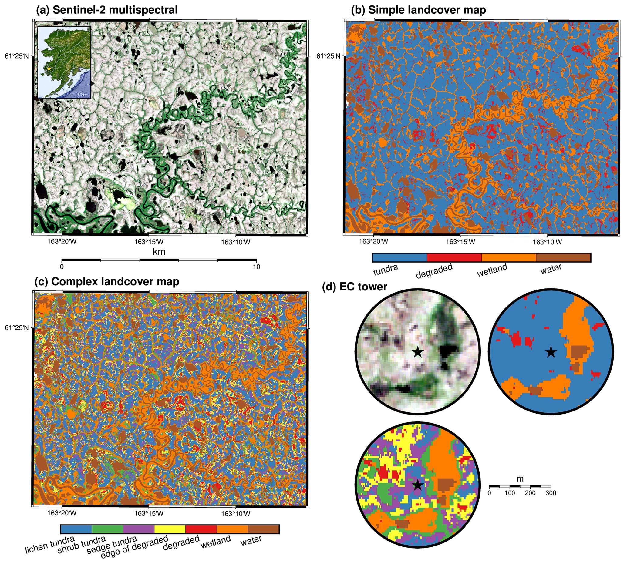
Figure 1 Scaling region within the YK Delta used in this study. Sentinel-2 RGB imagery (a) with the location of the grid within Alaska as an inset, simple land-cover map (b), and complex land-cover map (c). Panel (d) shows 300 m radius regions around the eddy covariance (EC) tower for the same Sentinel-2 RGB imagery as (a) in the upper left, the same simple land-cover map as (b) in the upper right, and the same complex land-cover map as (c) in the lower left. The EC tower is indicated by the star at 61.2548° N, 163.2589° W. Maps were created using the PyGMT software package; Wessel et al., 2019; Tian et al., 2024.

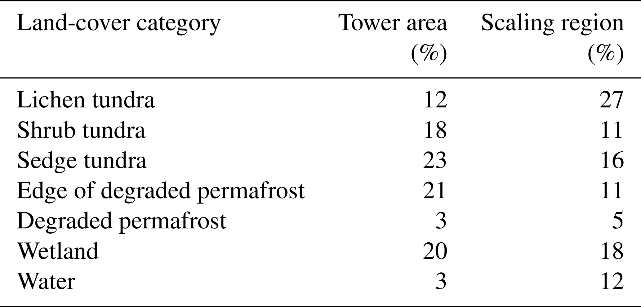
We used a land-cover map developed by Ludwig et al. (2022) to characterize the EC tower location and a nearby region of unburned tundra for scaling up the carbon budget (Ludwig et al., 2023a). The land-cover map is 5 m × 10 m resolution and derived from Sentinel-1 synthetic aperture radar (SAR), the Sentinel-2 multispectral instrument (MSI), and the ArcticDEM. Two versions of land cover were used: (1) a simple version with only four categories (surface water, tundra, wetland, and degrading permafrost) and (2) a complex version where tundra was further split into lichen tundra, shrub tundra, sedge tundra, and tundra at the edge of degrading permafrost (Fig. 1). Tundra land-cover categories were primarily located on peat plateaus and share the same dominant vegetation types of lichens, dwarf shrubs, mosses, and sedges. The differences within tundra categories were subtle. Shrub tundra was often located at the edges of peat plateaus bordering and along banks with slightly larger shrubs. Sedge tundra was located on peat plateau slopes that were slightly greener. Lichen tundra was the least green and largest area of tundra types within the region, dominated by lichen, moss (Sphagnum spp. and Dicranum spp.), and graminoids (Carex spp. and Eriophorum angustifolium) (Baillargeon et al., 2022). The edge of degraded tundra included tundra bordering degraded permafrost, often wetter, mossier, and slightly subsided. Degraded areas included isolated shallow depressions on peat plateaus, more evolved networks of flow paths draining peat plateaus into wetlands, and recently drained waterbodies. Depending on seasonality and antecedent rain, degraded areas could have standing water, saturated soils, exposed mud, or graminoid-dominated vegetation. The wetland category included a range of wetland vegetation such as mosses, graminoids, and tall shrubs, often with complex underlying hydrology. Wetland soils were usually saturated, with small, sub-pixel channels or waterbodies undetectable at the resolution of the land-cover map. Surface water includes all lakes, ponds, and streams detectable at the land-cover map resolution (Ludwig et al., 2023b). There are likely smaller ponds or channels within wetlands and degraded areas, but higher-resolution mapping would be needed to identify that level of heterogeneity. The full distribution of land-cover areas in a 300 m radius circle around the EC tower location and in the region used for scaling is described in Table 1. The scaling region was approximately 150 km², which is similar to the average size of a grid cell in Earth system models (Williams et al., 2009).

Table 1 Land-cover category percentages in the immediate eddy covariance tower area (radius of 300 m) and in the region used to scale up ecosystem carbon fluxes (Fig. 1).

2.2 Eddy covariance data processing

Data used in this study span from 12 July 2019 to 30 September 2020, though we only include May through September months. The EC tower instrumentation consisted of a Gill WindMaster Pro sonic anemometer, LI-7500DS open-path analyzer for CO₂ and H₂O, LI-7700 for CH₄, Vaisala HMP155 humidity and temperature probe, LI-190R quantum sensor for photosynthetically active radiation (PAR), Kipp and Zonen CNR4 four-component net radiometer, and HukseFlux HFP01SC soil heat plates. All instrumentation was connected to a LI-7550 interface equipped with a LI-COR SmartFlux system. The measurement height was 2.5 m above ground level. Half-hourly flux calculations were made using the eddy covariance method (Baldocchi et al., 1988) from 10 Hz data using the EddyPro software program (Fratini and Mauder, 2014). We used the double coordinate rotation method, spike removal, block averaging, and time lag removal by covariance maximization (Moncrieff et al., 1997). We made corrections for air density fluctuations for CO₂, CH₄, and H₂O fluxes following Webb et al. (1980). We removed fluxes with nonstationarity (flags of 2 in the overall flag system) (Mauder and Foken, 2015). We filtered fluxes to remove times of low signal strength (< 15 %) and low turbulence (friction velocity (u^∗) < 0.1 ms⁻¹ threshold was chosen where CO₂ fluxes were independent of u^∗). Energy balance closure at the site was typical (70 %). Lastly, we filtered fluxes to remove spikes using the double median absolute deviation method (Mauder et al., 2013). The resulting time series had 26 % and 61 % missing data for CO₂ and CH₄ fluxes, respectively. Due to limited access for site maintenance during the COVID-19 pandemic and the remote site location, power outages contributed to 1.5 % missing data in fluxes, air temperature, and PAR. While only actual observations of air temperature and PAR were used for training gap-filling models, we used a complete time series of drivers for scaling and to sum fluxes to monthly carbon budgets. To interpolate missing data in air temperature and PAR for scaling we used the marginal distribution sampling and mean diurnal course method from REddyProc (Wutzler et al., 2018). Annual time series of CO₂ fluxes, CH₄ fluxes, air temperature, and PAR observations can be found in the Supplement (Fig. S1a–d).

2.3 Eddy covariance footprint modeling

We compared three commonly used footprint models to determine source areas for fluxes: the Hsieh model (with the 2D extension from Detto et al., 2006), the Kljun model, and the Kormann and Meixner model (Hsieh et al., 2000; Kormann and Meixner, 2001; Kljun et al., 2015). The Hsieh model is a hybrid approach blending a forward Lagrangian stochastic numerical model with an analytical solution. The Kljun model uses multiple parameterizations of a backward Lagrangian particle model to be applicable across atmospheric stability regimes. The Kormann and Meixner model is an Eulerian analytical footprint model based on Monin–Obukhov similarity theory. All three footprint models assume Gaussian dispersion in the crosswind direction and horizontal homogeneity in turbulence effects (Schmid, 2002). Given the flat deltaic landscape and extremely short tundra canopy height relative to instrument measurement height, this site was an ideal location for footprint modeling, while still encompassing heterogeneity in CO₂ and CH₄ fluxes. We calculated a single roughness length for the site (0.02 m) from the measured wind speed and friction velocity under neutral conditions assuming a logarithmic wind profile and zero displacement height. For each half-hour flux observation, 1 m × 1 m grid footprints were generated using each of the three model types and then rotated into the wind direction. Each footprint was modeled 1000 m in the downwind direction and 250 m to either side in the crosswind direction. These values were chosen as they were well in excess of the 90 % contours of all footprints (peak influences were < 100 m and the 90 % contours averaged 200 m from the EC tower). These footprints were then reprojected to match the resolution and extent of the land-cover maps at 5 m × 10 m. Footprints were normalized to total 100 % by dividing by the sum of the weights within each observation. The footprint weights were then summed over each land-cover type (i) for each flux observation (k) as Ω_i,k (see Eq. 1 in Sect. 2.4.1).

2.4 Unmixing and gap-filling models

We compared several modeling approaches for predicting and gap-filling the EC NEE time series. First, we explicitly consider landscape heterogeneity by unmixing EC tower fluxes using each of the three types of footprint models when summarized over both the simple and complex land-cover map (Sect. 2.4.1). In order to do so, NEE fluxes were partitioned into respiration and gross primary productivity (GPP) with simple empirical models driven by PAR and air temperature. Second, we used the same method of flux partitioning, modeling, and parameter estimation to gap-fill NEE, but instead assumed a homogeneous landscape. Each of the heterogeneous types of gap-filling models and the similar homogeneous variation were trained separately for each month in the growing season (May through September) to accommodate seasonality. Observations from both 2019 and 2020 were used to train the gap-filling models, though we only predicted and scaled for 2020, since the 2019 growing season was incomplete. We tested the inclusion of 2019 observations for August and September, and there was little effect on the derived land-cover fluxes. Last, we compared these results to a widely used approach by gap-filling NEE with MDS, which implicitly assumes a homogeneous landscape. CH₄ fluxes were not as temporally variable as NEE and largely unrelated to biometeorological drivers measured at the EC tower (Fig. S2). CH₄ fluxes were subsequently treated as land-cover-specific constant fluxes through time and solved for separately in each month of the growing season, as has been done similarly in other studies (Rey-Sanchez et al., 2022; Tuovinen et al., 2019; Hannun et al., 2020).

2.4.1 Heterogeneous gap-filling models

Assuming that every pixel within a land-cover type is characterized by a similar flux, for a given (k) half-hour measurement, the observed EC tower NEE flux is the sum of each (i) land-cover flux (NEE_i,k) times the total influence of those pixels within a footprint (Ω_i,k) across all (P) land-cover types (Eq. 1).

$$\begin{array}{}\text{(1)}& {\mathrm{NEE}}_{\text{Obs},k}=\sum _{i=\mathrm{1}}^P{\mathrm{NEE}}_{i,k}\times {\mathrm{\Omega }}_{i,k}\end{array}$$

CO₂ fluxes are often highly variable in time, especially from vegetated environments. Tundra NEE has been well characterized as the difference between respiration – modeled as an exponential function of temperature – and gross primary productivity – modeled as a light-saturating response curve often attenuated by temperature or vapor pressure deficit (Williams et al., 2006; Shaver et al., 2007; Loranty et al., 2011). For the heterogeneous gap-filling models, we structured the (NEE_i,k) fluxes from vegetated land cover as temporally variable and dependent on air temperature (Tair_k), light (PAR_k), and air temperature rescaled between 0 and 1 (Tscale_k).

$$\begin{array}{}\text{(2)}& {\displaystyle }{\mathrm{NEE}}_{i,k}=R_{i,k}-{\mathrm{GPP}}_{i,k}\text{(3)}& {\displaystyle }{R}_{i,k}={\mathit{\alpha }}_i\times e^{{\mathit{\beta }}_i\times {\mathrm{Tair}}_k}\text{(4)}& {\displaystyle }{\mathrm{GPP}}_{i,k}={\mathrm{Tscale}}_k\times {\displaystyle \frac{{\mathrm{E}\mathrm{0}}_i\times {\mathrm{Pmax}}_i\times {\mathrm{PAR}}_k}{{\mathrm{Pmax}}_i+{\mathrm{E}\mathrm{0}}_i\times {\mathrm{PAR}}_k}}\text{(5)}& {\displaystyle }{\mathrm{Tscale}}_k={\displaystyle \frac{({\mathrm{Tair}}_k-T_{min})({\mathrm{Tair}}_k-T_{max})}{({\mathrm{Tair}}_k-T_{min})({\mathrm{Tair}}_k-T_{max})-({\mathrm{Tair}}_k-T_{\text{opt}}{)}^{\mathrm{2}}}}\end{array}$$

The parameters are the baseline respiration (α_i), the temperature sensitivity of respiration (β_i), the light-use efficiency of GPP (E0_i), and the maximum photosynthetic capacity (Pmax_i). GPP is attenuated by temperature using Tscale_k, where T_min = −1.5 °C, T_max = 40 °C, and T_opt = 15 °C (Luus and Lin, 2015; Luus et al., 2017; Schiferl et al., 2022). For the simple land-cover map, NEE fluxes from tundra, wetland, and degrading permafrost were all parameterized according to Eqs. (2) to (5). Surface water CO₂ fluxes were parameterized as a constant flux over time. While this is likely an oversimplification, a more complex lake emissions model was not feasible because the surface waters within the footprint were too small an area and too small in footprint influence to inform a more complex model. Similarly, for the complex land-cover map, all NEE fluxes from tundra land-cover types as well as from wetland and degrading permafrost were structured according to Eqs. (2) to (5) with water as a constant flux.

CH₄ fluxes were assumed to be constant over time for each land-cover type.

$$\begin{array}{}\text{(6)}& {\mathrm{CH}}_{\mathrm{4}\mathrm{Obs},k}=\sum _{i=\mathrm{1}}^P{\mathrm{CH}}_{\mathrm{4},i}\times {\mathrm{\Omega }}_{i,k}\end{array}$$

The only parameters in this simpler version of unmixing are the land-cover CH₄ fluxes themselves, CH_4,i, with the footprint influences (Ω_i,k) as the only time-variable driver (Eq. 6). All three footprint models were similarly compared for CH₄ fluxes. Only the complex land-cover map was used to unmix CH₄ fluxes, since the categories within tundra were known to be divergent, e.g., known very small fluxes from lichen tundra, while tundra at the edge of degraded could possibly be a large source (Ludwig et al., 2018b).

2.4.2 Parameter estimation and flux prediction

We unmixed EC tower fluxes to land-cover CH₄ and NEE_i,k fluxes by using a Bayesian analysis with Markov chain Monte Carlo (MCMC) simulation. We chose this method partly because unmixing approaches such as ordinary least squares (as used by Tuovinen et al., 2019) are not applicable with the nonlinear relationships used here between CO₂, air temperature, and PAR, and nonlinear least squares (as used by Rößger et al., 2019) assumes normal distributions for parameters and error variance, which is often not the case. In addition, there are several advantages to using a Bayesian approach to solve for land-cover fluxes. First, we can provide prior information on flux parameters. This prior information could be specific (e.g., from chamber fluxes from land cover within the footprints), it could be more general (e.g., dictating one land cover known to have higher GPP than another), or it could be mostly uninformative and merely place restrictions on parameter space based on physical properties (e.g., non-negative Pmax_i). We used the latter approach to NEE priors for this study to demonstrate the impacts of unmixing EC tower NEE on gap-filling accuracy and bottom-up scaling while using the fewest assumptions. Given the simpler approach used to unmix CH₄ fluxes, there were multiple solutions if all prior fluxes were strictly uninformative. We used mostly uninformative prior fluxes for land cover known to emit CH₄ (e.g., fully saturated soils and open water) by disallowing CH₄ uptake for degraded, edge of degraded, wetland, and water land-cover classes (Ludwig et al., 2018a). Peat plateau chamber flux measurements from 2017 demonstrate a very small but nonzero CH₄ flux at the driest time of the growing season (Ludwig et al., 2018b), and we assigned prior fluxes for tundra types accordingly. Prior distributions can be found in the Supplement (Tables S1–S3). The second benefit of using Bayesian analysis with MCMC is that derived quantities and predictions of new data are inherently treated as random variables with their own probability distributions, thus enabling easy calculations of uncertainties. Therefore, we carry through uncertainty from both partitioning and gap filling to uncertainty in predicted land-cover NEE_i,k or CH₄ fluxes, which, when summed over time and scaled up by area, leads to distributions of carbon budgets from which we can calculate explicit uncertainties.

For each month of the growing season (May to September), gap-filling models were fit separately for each footprint type and land-cover map combination. First, NEE_Obs,k values were filtered to dark data (PAR < 50 $\mathrm{\mu }\mathrm{mol}{\mathrm{m}}^{-\mathrm{2}}{\mathrm{s}}^{-\mathrm{1}}$) and respiration parameters (Eq. 3) were determined while using uninformative priors. The GPP parameters (Eq. 4) were then estimated using the NEE_Obs,k from the full dataset, with uninformative GPP priors but using the posterior distributions of the respiration parameters as strict prior information for the respiration component of Eq. (2). CH₄ fluxes were fit separately by month as well, but all times of day were used. We used a Gibbs sampler for the MCMC iterations (Just Another Gibbs Sampler; JAGS) implemented with the runjags R package (Denwood, 2016), with a burn-in of 5000 iterations and an adaptation of 5000 iterations, and we retained 3000 iterations in the final chains. Three parallel chains were used for each model with different initial parameter values (Tables S1–S3). We evaluated parameter convergence using the Gelman diagnostic (Gelman and Rubin, 1992; Brooks and Gelman, 1998). Model performance was further checked using posterior predictive checks of the mean, standard deviation, and sum of squared residuals (Gelman et al., 1996).

2.4.3 Homogeneous gap-filling models

We used several methods to gap-fill the EC tower NEE and CH₄ fluxes that both assume a homogeneous landscape and footprint for comparison. The first method is a Bayesian analysis with MCMC sampling that mirrors our land-cover flux unmixing approach in every way except by assuming a homogeneous landscape. For the homogeneous Bayesian model, we assume a single land-cover type everywhere that accounts for 100 % of the footprint influence at every flux observation. The homogeneous land-cover NEE was modeled monthly by Eqs. (2) to (4), with the same partitioning and parameter estimation as described in Sect. 2.4.2. The second homogeneous NEE gap-filling approach we used was MDS (Reichstein et al., 2005). We used the REddyProc package with default settings to implement the MDS gap filling (Wutzler et al., 2018). Since the CH₄ fluxes did not have relationships to observed biometeorological drivers such as air temperature or PAR (Fig. S2), we estimated monthly budgets by calculating the monthly average CH₄ flux for each half-hour of the diurnal cycle and then applying these averages to each day within the month.

2.4.4 Artificial gaps

Artificial gaps in the NEE and CH₄ flux observation time series were created in order to be able to evaluate and compare gap-filling approaches. Since the MDS gap-filling method requires at least 90 d of half-hourly measurements, it could only be applied to the 2020 growing season (data in 2019 began in mid-July). Therefore, we only created artificial gaps in the 2020 growing season for comparability. Artificial gaps were generated separately for each month to ensure each portion of the growing season had a similar amount of withheld data. Between 15 % and 20 % of the time series of each month was withheld as random artificial gaps of stratified sizes, with ≈ 5 % as larger gaps (10 observations), ≈ 5 % as smaller gaps (4 observations), and the remainder as single gaps. The withheld drivers corresponding to the artificial gaps (PAR, air temperature, footprint weights) were then used to predict EC tower NEE or CH₄, and gap-filling methods were evaluated by calculating the root mean square error (RMSE).

2.5 Scaling up NEE and CH₄

We used the parameter posterior distributions from MCMC simulations and full time series of air temperature and PAR to predict complete, gap-filled CH₄ and NEE_i,k flux time series for the land-cover types as described in Sect. 2.4.2. We then summed these distributions of half-hourly fluxes over time and multiplied by their respective areas in the scaling region (Sect. 2.1, Fig. 1) to determine estimations of monthly carbon budgets for each land-cover type. Monthly land-cover carbon budgets were calculated for each footprint model and land-cover map combination. Land-cover carbon budgets were then summed to create monthly and growing season carbon budgets for each footprint model and map type. Monthly and growing season carbon budget distributions for the Bayesian homogeneous gap-filling models were similarly estimated. The observed EC tower NEE fluxes with MDS gap filling were also summed over time and multiplied by the total scaling region to arrive at comparative monthly carbon budget estimates. CH₄ was presented alongside NEE in carbon budgets as CO₂ equivalents (CO₂-eq) by multiplying by a factor of 28, a conservative choice among commonly used approximations of relative global warming potentials (Bastviken et al., 2011; Stocker, 2013; Euskirchen et al., 2014; Beaulieu et al., 2020; Skytt et al., 2020). For discussion of uncertainty in carbon budgets, we calculated 89 % Bayesian credible intervals (CIs), which are analogous to frequentist 95 % confidence intervals (Kruschke, 2014; McElreath, 2015; Hobbs and Hooten, 2015), using the highest-density interval method from the “baysetestR” package (Makowski et al., 2019).

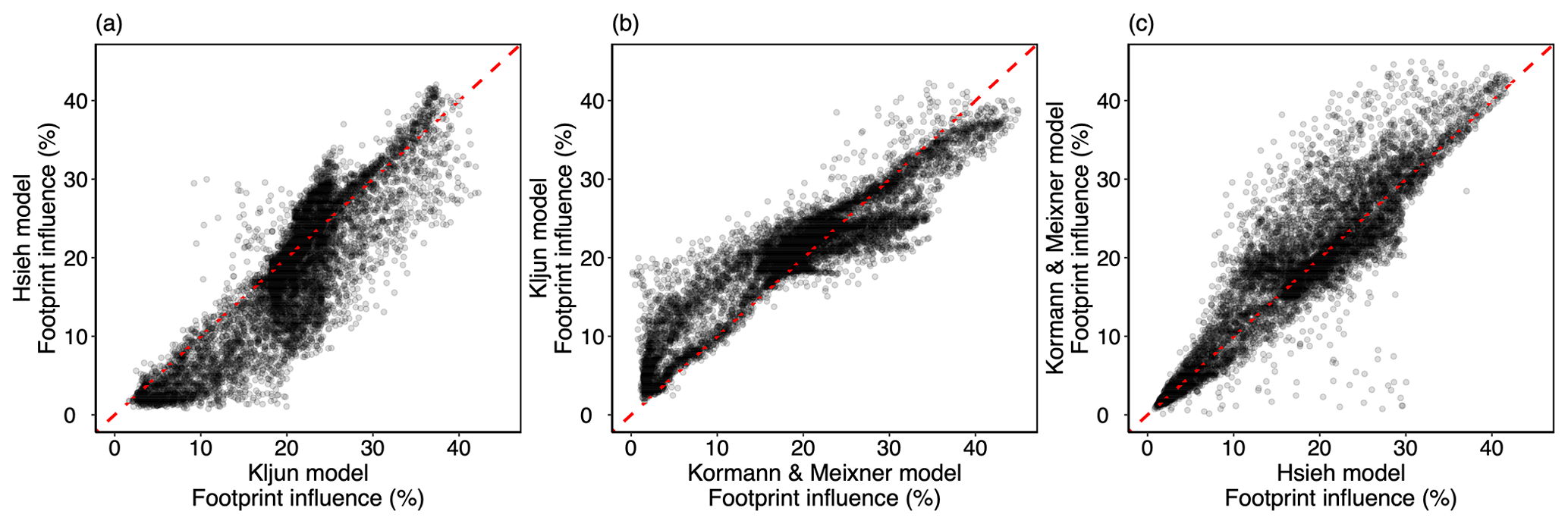
Figure 2 Scatterplot demonstrating comparison of footprint influence weights between the three models (Hsieh, Kljun, Kormann–Meixner) for lichen tundra. Other land-cover footprint influence comparisons can be found in the Supplement (Fig. S3). The dashed red line indicates the 1:1 line.

3 Results and discussion

3.1 Footprint influence

The most common and most influential land cover within the footprints was tundra, averaging 70 % influence over the growing season for all three footprint model types. There was a fairly even distribution between tundra category types, though sedge tundra had slightly more influence than lichen, shrub, and degraded edges. The footprint influence from wetlands was comparable to that of individual tundra types. The least represented land cover types were degraded permafrost and surface water, both of which were between 0 % and 20 % influence (Fig. S3). The vast majority of footprints were a mix of land-cover types, with almost no individual footprints having a land-cover type with more than 75 % influence (Fig. S3). There was a fair amount of agreement between the three footprint models, with the majority of footprint influences close to the 1:1 line on regressions between model types (Figs. 2 and S3). Other studies that have sought to compare the ability of these footprint models to recover known flux sources have found little distinction between them, despite the differences in their methodology (Coates et al., 2021; Rey-Sanchez et al., 2022). However, the land-cover influences used here were sums of all pixel influences within a land-cover type; therefore, small differences between models on a pixel basis were cumulative and would lead to larger discrepancies overall. There are also distinct periods of larger differences between footprint models, for example when the peak footprint influence was near the boundary between two land-cover types; thus, a small shift in peak location between model types would lead to a large difference in land-cover influences. A higher-resolution land-cover map (e.g., 3 m or smaller) would minimize some footprint model discrepancies, though this is relative to the extent of the footprints and the scale of landscape heterogeneity affecting carbon fluxes.

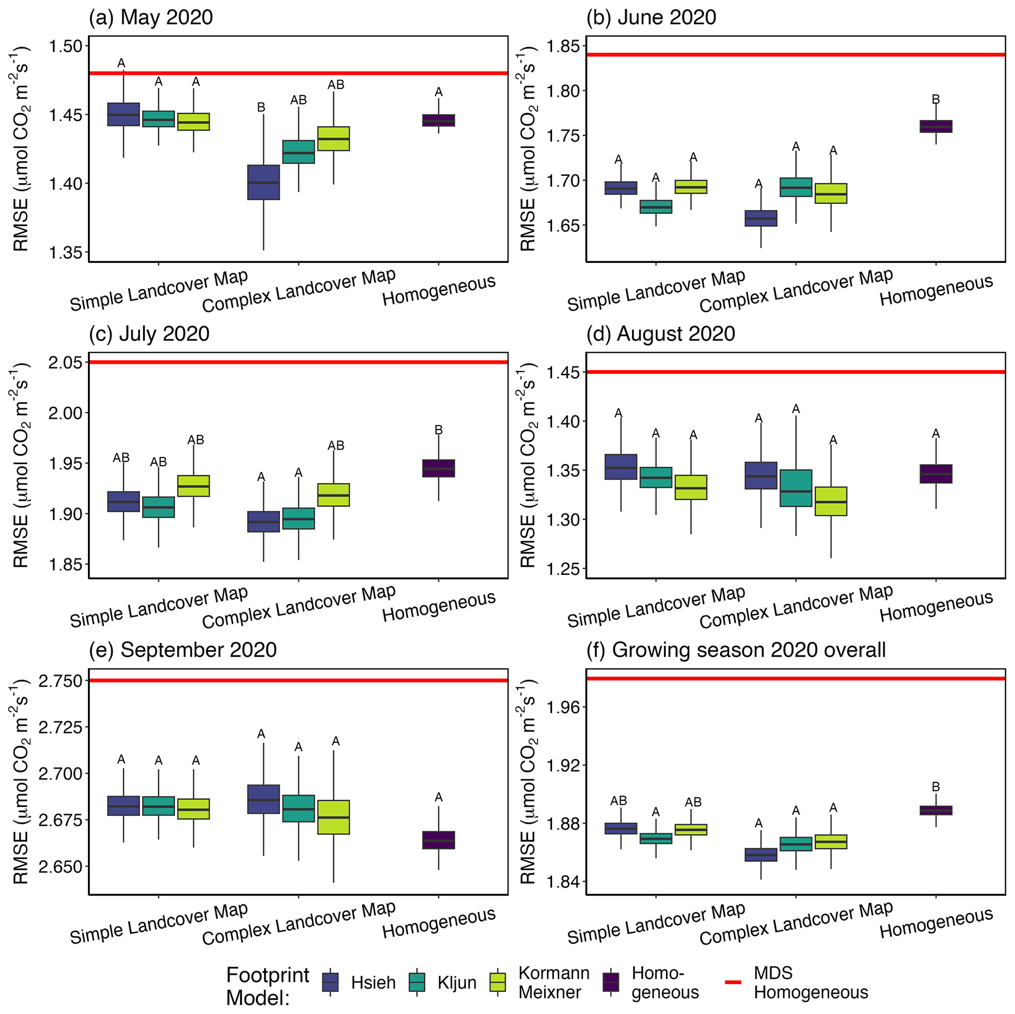
Figure 3 Monthly RMSE (a–e) and growing seasonal total (f) for 2020 from artificial gap-filling NEE fluxes. Boxes are the median and interquartile range (IQR), and whiskers are 1.5 ⋅ IQR for the Bayesian model gap-filling RMSEs. The red line indicates MDS (marginal distribution sampling) gap-filling RMSEs. Distributions with overlapping Bayesian 89 % credible intervals are designated with matching letters. Note that the scales on y axes are different between panels to highlight the comparability of footprint models and land-cover maps within months.

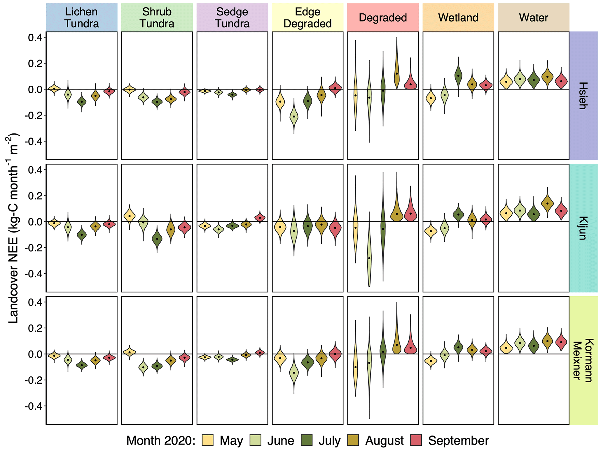
Figure 4 Monthly violin plots of predicted NEE fluxes from the 2020 growing season by land cover (columns) for each of the three footprint models (rows) using the complex land-cover map to unmix the EC tower fluxes. Distributions for violin plots are derived from posterior distributions of predicted NEE. Black dots indicate medians.

3.2 Model performance

All posterior predictive checks were passed (Bayesian p-values of 0.1 < p < 0.9), and all parameters converged (Gelman diagnostics ≈ 1) for every Bayesian gap-filling model. All Bayesian gap-filling models were able to accurately reconstruct the EC tower NEE across the growing season as a function of PAR, air temperature, and source attributions (Figs. 3 and S4). The only notable deviations were exclusive to outliers in EC tower NEE observations. This result is not unexpected, as EC data are often noisy. Mismatch with EC tower NEE outliers could also be a consequence of processes dominating fluxes that were not represented in our models, e.g., high CO₂ emissions from ebullition aligning with high lake influence within a footprint. When comparing performance for filling the same artificial gaps, all Bayesian models had a lower (better) RMSE than the MDS method (Fig. 3). The Bayesian models, both heterogeneous and homogeneous, drive NEE as deterministic functions of PAR and temperature. This may be why they were more accurate than MDS, which has been shown to be biased in high latitudes due to the effects of skewed distributions of net radiation (Vekuri et al., 2023). The heterogeneous gap-filling models often performed better than their homogeneous equivalent (Fig. 3). For most months, the heterogeneous complex map solutions had lower RMSEs than those of the simple map, though the Bayesian 89 % CI overlapped between all months but May (Fig. 3). In May near the shoulder season, tundra types exhibited greater differences in seasonality. For example, the lichen tundra had very little GPP, while the sedge tundra was a distinct carbon sink (Fig. 4), and this could be accommodated in the complex map while the simple map attempted to fit both to a single “tundra” flux. While there were clear improvements in gap-filling RMSE using this unmixing method, the differences in RMSE were small relative to the magnitude of the fluxes. The drawbacks of the flux unmixing method used here are site-specific solutions and longer computation times, which increase with the landscape complexity considered. MDS remains faster to implement and could be preferred when landscape homogeneity can be safely assumed.

None of the three footprint models consistently performed better in terms of RMSE, and for most outcomes, the Bayesian 89 % CIs for their RMSEs overlapped (Figs. 3 and S5). Given that none of the three footprint model types quantify their uncertainty, we continued to evaluate all three as an ensemble of footprint models that represents the range in footprint influence outcomes. Another way to evaluate performance of the three footprint models is by comparing their consistency in predicting land-cover NEE fluxes when the underlying land-cover map switches from simple to complex. The degraded permafrost, water, and wetland land-cover types were identical between the two maps and ideally should have the same derived fluxes even if the tundra categories were treated differently. Similarly, the overall tundra footprint-weighted flux should match between simple and complex land-cover types, even though the complex tundra was a combination of four types where there was only one tundra type for the simple map. By weighting the predicted land-cover NEE by their respective footprint influences for each observation, we regressed the simple vs. complex solutions (Figs. S6–S10). While the EC tower NEE and tundra total weighted NEE were very consistent between land-cover maps for all footprint models, the Hsieh and Kormann–Meixner models were notably inconsistent for degraded permafrost for June and July (Figs. S7 and S8), while the Kljun footprint model was always distinctly consistent (Figs. S6–S10). This outcome might indicate that the Kljun footprint model was more representative of land-cover influences at peak growing season. In the absence of extensive concurrent chamber fluxes to conclusively distinguish between derived land cover types from the footprint models, we recommend a footprint model ensemble approach.

Figure 5 Monthly violin plots of CH₄ 2020 growing season budgets by land cover (columns) for each footprint model (rows). Distributions for violin plots are derived from posterior distributions of predicted CH₄ fluxes scaled by their land-cover areas in Fig. 1. Black dots indicate medians.

3.3 Derived land-cover fluxes

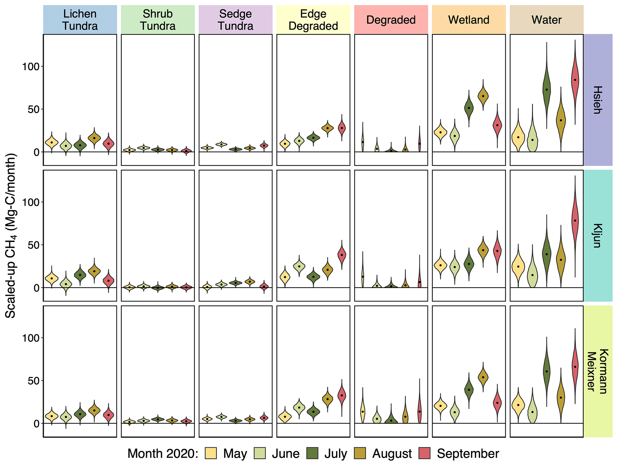
There was enough similarity between footprint model influences to yield similar patterns in derived land-cover fluxes (Figs. 4 and S11, Tables S4–S10). For example, in all three footprints both shrub tundra and tundra at the edge of degrading permafrost had higher peak carbon uptake (−0.342, −0.266, −0.308 $\mathrm{kg}\mathrm{C}{\mathrm{month}}^{-\mathrm{1}}{\mathrm{m}}^{-\mathrm{2}}$, for Hsieh, Kljun, and Kormann and Meixner, respectively) than sedge and lichen tundra (−0.175, −0.175, −0.139 $\mathrm{kg}\mathrm{C}{\mathrm{month}}^{-\mathrm{1}}{\mathrm{m}}^{-\mathrm{2}}$, for Hsieh, Kljun, and Kormann and Meixner, respectively) (Fig. 4). This aligns with previous studies that have found higher productivity in shrub tundra and areas adjacent to disturbed tundra, possibly the result of increased nutrient availability (Schuur et al., 2007; Bowden et al., 2008; Lee et al., 2011). The range of NEE fluxes derived for tundra vegetation was similar to ranges in NEE observed at other tundra sites (Euskirchen et al., 2012; Howard et al., 2020; Virkkala et al., 2022). All three footprint models also derived higher CO₂ and CH₄ emissions from surface water and wetlands later in the growing season (Figs. 4 and 5), which could be the result of increased thaw depths contributing to greater lateral carbon transport from peat plateaus. Pore-water dissolved organic carbon and dissolved CO₂ and CH₄ were extremely high on peat plateaus during the growing season (Zolkos et al., 2022), and open waters in both wetlands (sub-pixel) and waterbodies were likely hot spots for decomposition and outgassing (Ludwig et al., 2022). The wetlands were also characterized by deep, carbon-rich soil, which could be contributing to higher baseline respiration (Fig. 4, Table S9). The derived CH₄ fluxes from land-cover classes in this study were within the ranges reported in the Boreal–Arctic Wetland and Lake Dataset (BAWLD-CH₄), including from wetlands and the edge of degraded permafrost (wetlands and wet tundra in BAWLD), peat plateaus (dry tundra in BAWLD), and waterbody CH₄ fluxes (small peatland lakes in BAWLD) (Kuhn et al., 2021). The CO₂ fluxes reported here are similar in range to those observed in small ponds in other sub-Arctic tundra ecosystems (Kuhn et al., 2018).

The three footprint models followed similar patterns in peat plateau seasonality as well, with NEE uptake peaking in July for most tundra types (Fig. 4). Lichen and sedge tundra were very small CH₄ sources (Fig. S11), though given the large area of lichen tundra in the landscape this resulted in a notable contribution to total CH₄ (Fig. 5) when scaling up. Shrub tundra was either zero or a very small CH₄ source, depending on the footprint model (Fig. 5). Tundra at the edge of degrading permafrost was a significant CH₄ source and behaved more similarly to wetlands than degraded areas in terms of seasonal patterns (Fig. 5). Interestingly, degraded permafrost was a sink of CO₂ earlier in the growing season (Fig. 4), but all GPP parameters converged to zero in August and September (Fig. 4, Table S8). Degraded permafrost was a source of CH₄ early in the growing season, decreased to near zero as the depressions dried down, and then increased again later in the growing season (Figs. 5 and S11). This aligns with the wettest portion of the growing season, when the small depressions of degrading permafrost become inundated as small ponds (Mullen et al., 2023), which could explain the renewed CH₄ emissions and decline in GPP.

There were differences as well between the derived land-cover fluxes for the three footprint models. These differences were offsetting between adjacent land-cover types. For example, degrading permafrost and tundra at the edge of degrading permafrost were always, by definition, near one another. When the Kljun model had high CO₂ uptake in degrading permafrost it had lower uptake at the edge of degrading permafrost, whereas Hsieh and Kormann–Meixner displayed the opposite pattern (Fig. 4). This discrepancy was the result of slight differences between footprint models in peak influence positioning at the boundary of the two land-cover types (Figs. 2 and S3). The differences in effects of the footprint models can likely be minimized by using a relatively higher-resolution map or including spatial drivers such as leaf area index (LAI), soil moisture, and soil temperature, which would provide further constraints for land-cover fluxes.

The complex heterogeneous models captured distinctive seasonality. Lichen and shrub tundra were net neutral in May, had peak CO₂ uptake in July, and remained small sinks in September (Fig. 4). In contrast, the sedge tundra and edge of degrading permafrost were small sinks in May, peaked earlier, and were net neutral or CO₂ sources by September (Fig. 4). Increasing the complexity of the underlying map allowed us to determine this separate but ecologically significant seasonality in peat plateau CO₂ cycling. However, there is a limit to how complex one can get. The land-cover map used in this study identified two types of wetlands, one much more prevalent near the EC tower than the other. Attempting to use both wetland types failed, as the parameters for the less prevalent wetland could not converge. We subsequently lumped both wetland categories as “wetland”. This failure to converge serves as a check against over-fitting, which can be used in addition to comparing against withheld data via artificial gaps. In the event that a land cover with small area or influence is significant to the research questions posed and this unmixing method cannot derive a flux, then we recommend supplying stricter prior information for the land cover via chamber fluxes. By combining chamber fluxes and EC tower flux unmixing, one can leverage both the spatial coverage and temporal frequency of EC tower fluxes with the specificity of chamber fluxes.

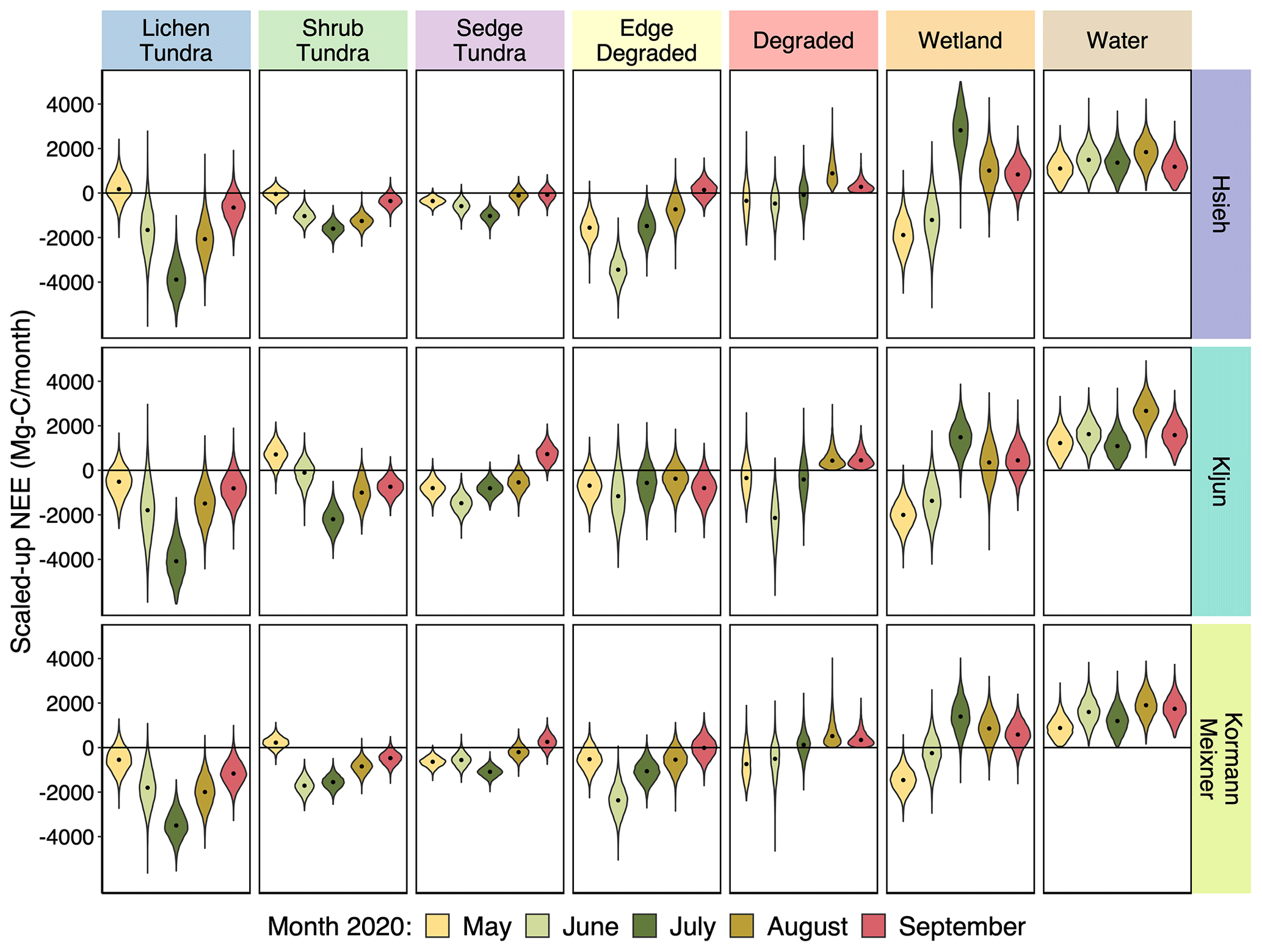
Figure 6 Monthly violin plots of 2020 growing season NEE carbon budgets by land cover (columns) in the complex map for each footprint model (rows). Distributions for violin plots are derived from posterior distributions of predicted NEE fluxes scaled by their land-cover areas in Fig. 1. Black dots indicate medians.

3.4 Land-cover scaling

Scaling up fluxes to the region led to distinct land-cover hot spots of carbon sinks and sources, with all three footprint models having similar monthly NEE and CH₄ budgets by land-cover type (Figs. 5 and 6). Lichen tundra was the largest sink of carbon (the 89 % CI of July carbon uptake was −2628 to −5075 Mg C for the Hsieh model, −2715 to −5452 Mg C for the Kljun model, and −2493 to −4428 Mg C for the Kormann and Meixner model), though this was driven in part by occupying the largest area in the region (Fig. 1; Table 1). Wetlands and surface waters were significant sources of both CO₂ and CH₄ in the latter half of the growing season (July–September), with large enough emissions to offset the carbon uptake in some of the peat plateau land cover types (Figs. 5 and 6). Wetlands account for, on average, only 7 % of what the EC tower sees, but 18 % of the area in the region. If we were to use a coarser land-cover map, such as the recently updated circumpolar Arctic vegetation map (CAVM) (Raynolds and Walker, 2022), we would have attributed 100 % of the EC tower fluxes to wetland complex vegetation, which would scale up to 26 % of the region using CAVM. Given the clearly distinctive carbon dynamics between wetlands and peat plateau vegetation, using a land-cover resolution appropriate to the scale of heterogeneity is important for obtaining an accurate regional carbon budget and understanding the ecosystem.

Regional surface water carbon emissions scaled up from the EC tower fluxes are likely an overestimate, since the waterbodies within the EC tower footprints were amongst the two smallest size classes of waterbodies in the region, which have the largest diffusive carbon fluxes (Ludwig et al., 2023b). In comparison, the coarser CAVM land-cover map does not identify any surface waters in the entire scaling region, which would lead to these hot spots of emissions being completely underestimated. Scaling up surface water carbon emissions would be better done using an approach that includes both terrestrial and aquatic landscape drivers and uses better spatial representation (e.g., Ludwig et al., 2023b) than the area seen by a single EC tower. However, we were able to capture both plant-mediated carbon fluxes and ebullition in addition to diffusive fluxes, as well as describe the broad seasonal trends in carbon emissions using this approach.

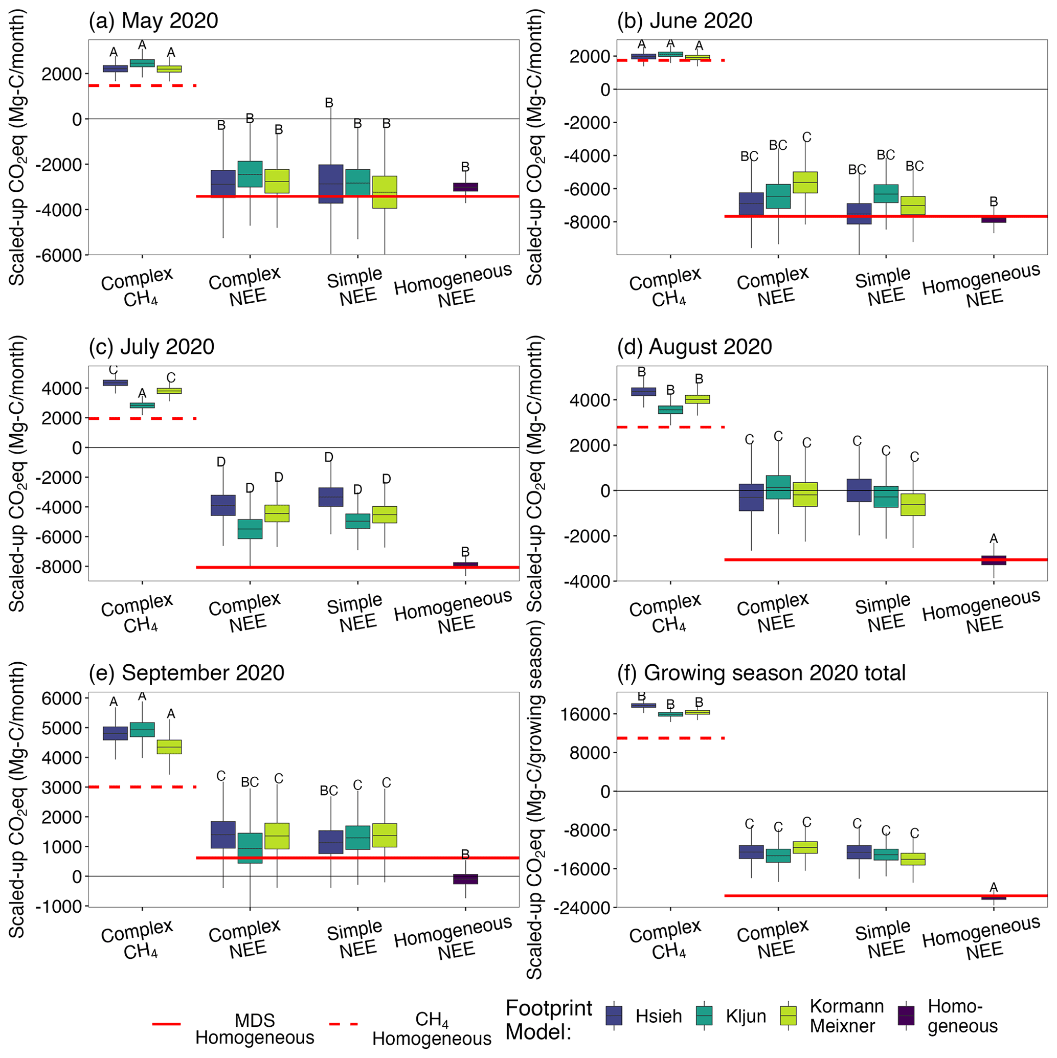
Figure 7 Monthly total (a–e) and 2020 growing season total (f) CO₂-eq carbon budgets for each gap-filling technique. Boxes are the median and interquartile range (IQR), and whiskers are 1.5 ⋅ IQR for the Bayesian model gap-filling carbon budgets using the three footprint models over the complex and simple land-cover maps, as well as without considering footprints and assuming a homogeneous landscape. The solid red line indicates MDS (marginal distribution sampling) homogeneous gap-filling NEE budgets. The dashed red line indicates the diurnal average CH₄ gap-filling homogeneous budgets. Distributions with overlapping Bayesian 89 % credible intervals are designated with matching letters. Note that the scales on y axes are different between panels to highlight the comparability of footprint models and land-cover maps within months.

3.5 Regional carbon scaling

Land-cover carbon budgets were summed to regional carbon budgets and compared to carbon budgets estimated using the Bayesian and MDS homogeneous approaches (Fig. 7). Total NEE was similar between the three footprint models with overlapping 89 % CI. Regional CH₄ budgets were also similar, with most months overlapping 89 % CI between the three footprints and a small difference in July. There was also no difference in total NEE budgets between the simple and complex map solutions. For most months the complex map solutions were slightly more uncertain, a consequence of estimating almost twice as many parameters and carrying through all of their uncertainties. The exception was May, for which the simple map was more uncertain, likely because grouping all tundra vegetation as one class was a poor assumption for that time. Despite the differences in methodologies, the two homogeneous approaches (Bayesian models and MDS) resulted in very similar NEE budgets to one another when scaling up to the region for June, July, and August (Fig. 7). In months closer to the shoulder season (May and September), the distributions of light and temperature were more skewed, which can be a source of bias in the MDS method and could explain the slight differences in the MDS and Bayesian homogeneous results for those months.

In contrast, all homogeneous scaled-up carbon results were quite different from the heterogeneous results. While the homogeneous approaches were worse at predicting to withheld gaps in the EC tower observations (Fig. 3), the differences in RMSE were small. However, the consequences for scaling were large. At every part of the growing season the homogeneous NEE overestimated the carbon sink relative to the heterogeneous NEE. This overestimation was smaller towards the shoulder seasons in May and September and larger in June, July, and August. Assuming homogeneity at this site meant approximating the same diurnal cycle of NEE everywhere that averages over different sink and source strengths in the landscape. Similarly, assuming a homogeneous landscape when scaling up an average CH₄ flux led to consistently underestimating the regional CH₄ emissions (Fig. 7). Because land-cover types that were hot spots of emissions were farther from the footprint influence peaks, while those that exhibited larger carbon uptake were more often nearer the peaks, applying the EC tower flux to the region without accounting for footprints resulted in too much carbon uptake in NEE and too little carbon emission in CH₄.

Throughout the growing season, incorrectly assuming a homogeneous landscape, regardless of gap-filling methodology, resulted in nearly doubling the NEE growing season carbon sink while nearly halving the CH₄ emissions (Fig. 7f). If we had assumed a homogeneous landscape we would have determined the region to be a net growing season carbon sink even after accounting for CH₄ emissions as CO₂ equivalents (89 % CI: −9960 to −11 919 Mg C, Fig. 7f). We can combine the posterior distributions of scaled carbon from all three footprint model results to calculate a single CO₂-eq carbon budget estimate that accounts for across-model uncertainties. Doing this, we find that growing season CH₄ emissions (mean: 16 633, 89 % CI: 15 208 to 18 212 Mg C CO₂-eq) more than offset the CO₂ growing season sink (mean: −12 512, 89 % CI: −15 718 to −9189 Mg C). Similarly, Kuhn et al. (2018) found that accounting for emissions from commonly overlooked small ponds offset much of the wetland carbon sink in northern Sweden. Other EC tower flux sites might see similar or opposite results from accounting for footprint heterogeneity (Griebel et al., 2016; Giannico et al., 2018; Reuss-Schmidt et al., 2019). A heterogeneous site with low carbon uptake or high carbon emissions located near the peak of footprint influences would overestimate carbon emissions when scaling assuming homogeneity. Unaccounted-for heterogeneity such as this could help explain the mismatch between bottom-up and top-down carbon budgets (Thornton et al., 2016; Saunois et al., 2020).

3.6 Uncertainty

A benefit of using this Bayesian approach is that uncertainties in model fit for respiration, GPP, and constant fluxes were carried through into uncertainties in NEE and CH₄ gap-filling and scaled-up carbon budgets. Sources of uncertainty included times and locations at which the deterministic models used here were oversimplifications and failed to capture other important processes affecting carbon cycling. Instances in which the land-cover maps were not accurate delineations of carbon cycling are also included in this uncertainty. For example, if an underlying gradient of soil moisture were causing different CH₄ fluxes within a vegetation type this would lead to greater uncertainty after the aggregation of footprint influences over the categorical map used here. Not all land-cover carbon budgets were equal in terms of uncertainty; for example, among the tundra vegetation types, NEE fluxes from the edge of degraded areas were the most uncertain, followed by shrub, lichen, and sedge (Fig. 4, e.g., Kljun–June standard deviations: 0.061, 0.031, 0.030, and 0.016 $\mathrm{kg}\mathrm{C}{\mathrm{month}}^{-\mathrm{1}}{\mathrm{m}}^{-\mathrm{2}}$, respectively). After scaling up to the region in (Fig. 1), lichen NEE carbon budgets were the most uncertain due to their larger area in the region, followed by the edge of degraded permafrost, shrub, and then sedge tundra (Fig. 6, e.g., Kljun–June standard deviations: 1199, 1009, 516, and 388 Mg C month⁻¹, respectively).

Degraded permafrost NEE and CH₄ fluxes had the most uncertainty (Figs. 4 and S11). This was likely due to a combination of their small extent and influence in the footprint supplying less signal to the EC tower fluxes, as well as the deterministic models oversimplifying carbon processes. In this case, the fluxes from degraded permafrost were distinctive enough that they could be determined while unmixing the EC tower fluxes despite their small area in the footprints. Within the areas of degrading permafrost there was heterogeneity in vegetation and surface water on a scale smaller than the resolution of the land-cover maps, as well as more temporal dynamics related to hydrology. Similarly, NEE and CH₄ fluxes from water had relatively large uncertainty due to estimating an average flux rather than presenting diffusive, plant-mediated, and ebullitive fluxes deterministically. In lieu of representing these processes explicitly, our simpler models had greater uncertainty. The uncertainty around degraded NEE and CH₄ fluxes had a smaller impact on NEE carbon budgets than other land cover types (Figs. 5 and 6) due to the small area of degraded locations in the landscape (Fig. 1). Since all of the uncertainties in gap-filling fluxes and partitioning NEE were carried through into carbon budget estimates, we lose nothing by including these small areas of heterogeneity despite not representing them as well as other land-cover types.

3.7 Applications and limitations of unmixing eddy covariance fluxes

Heterogeneity within EC tower landscapes is a common problem, and employing this flux unmixing approach at sites such as those identified by Chu et al. (2021) could improve accuracy in scaling carbon budgets and benchmarking models. Several studies have used summed spatial variables after weighting by EC footprints to relate to EC flux observations (Reuss-Schmidt et al., 2019; Xu et al., 2017; Metzger et al., 2013). While a useful way to incorporate heterogeneity, this approach reduces meaningful variation of spatial variables within footprints to single non-unique results. For example, there are multiple combinations of footprint weights and values of the spatial drivers that could result in the same weighted sum. Statistically unmixing fluxes could yield more informative relationships to spatial drivers.

Future applications of the flux unmixing approach demonstrated in this study could incorporate spatially explicit drivers such as soil moisture and soil temperature, as well as more specific prior information from chamber fluxes. Doing so would further reduce uncertainty in landscape carbon fluxes. Seasonality could be represented through spatially explicit and temporally variable drivers such as solar-induced fluorescence (SIF) (Luus et al., 2017; Schiferl et al., 2022). Interannual variability could be investigated using a hierarchical model structure by, for example, fitting an underlying distribution of a vegetation-type-specific Q₁₀ from which each year's specific Q₁₀ is drawn. This method of interpreting EC fluxes could also be useful at sites with nested EC towers, multiple instrument heights, or where instrument heights have changed over time (e.g., Klosterhalfen et al., 2023). Flux data from such circumstances could be analyzed concurrently, since each observation is a function of an explicit footprint distribution. Thus, it would not matter if instrument height or position were different between observations.

An alternative model structure for GPP was investigated that uses leaf area index (LAI) as a driver (Shaver et al., 2007). In lieu of field-based LAI data, we used a time series of NDVI from cloud-free Sentinel-2 imagery and the empirical relationship to LAI from pan-Arctic tundra described in Shaver et al. (2013). The LAI-version GPP model failed posterior predictive checks for most months of data and was not further pursued. This failure is likely because the approximation from NDVI was a poor representation of LAI for this site, particularly during May, August, and September when sub-pixel water presence could lead to erroneous NDVI and LAI. Furthermore, lichen and moss species dominated the vegetation biomass on peat plateaus and LAI may not be an appropriate metric in such cases. However, a spatially resolved driver such as LAI might be effective in applications for unmixing NEE at other sites.

This method of unmixing EC fluxes relies upon accurate footprint influence maps with sufficient variability over the heterogeneity in the landscape. The analysis in this study assumes that the footprints were observed perfectly; i.e., footprint influence is not a random variable. For this reason, we recommend always using an ensemble of footprint models. However, for sites where the assumptions of footprint models are not met and footprint influence maps are likely to be more error-prone, this study's methodology will not work. Examples of such cases might include sites with instrument heights close to canopy heights where the effects of the surface roughness sub-layer are a concern or anywhere the assumption of horizontal homogeneity in turbulence is invalid. In addition to valid footprint influences, this method requires variability in footprints. When footprint influences are aggregated over a land-cover type for unmixing, there need to be enough differences between observations to avoid an underdetermined dataset, where finding a solution to land-cover-specific fluxes will not be possible. Sites with consistent wind directions and atmospheric stability that result in very similar footprints between observations could have this issue. Small changes in the peak influence location could create enough variability between observations, even with consistent wind directions, depending on the position and scale of heterogenous land-cover patches at the site.

4 Conclusions and implications

We compared multiple footprint models and land-cover maps in our analysis to investigate their effects on unmixing land-cover carbon fluxes. While the Kljun footprint model was the most consistent in determining fluxes when comparing outcomes using simple and complex land-cover maps, there was no clearly best footprint model. We recommend including all three footprint models as an ensemble when interpreting EC fluxes. Flux estimates based on the more complex land-cover map captured important differences in seasonality in tundra vegetation carbon fluxes. However, there were only minor differences in regional growing season carbon budgets between the two land-cover maps, and using the more complex map had trade-offs such as greater computation time and uncertainty due to increasing the number of parameters. Investigating carbon fluxes using multiple land-cover maps allows for informed lumping of land-cover classes based on the resulting fluxes and the investigator's research questions.

Eddy covariance towers provide a wealth of high-frequency flux data with large spatial extents. However, EC tower fluxes are under-utilized or potentially misleading if footprints are not taken into account in heterogeneous landscapes. We have demonstrated an approach to unmixing EC tower NEE and CH₄ fluxes from heterogeneous tundra, which provided detailed interpretations of landscape carbon cycling such as the detection and quantification of hot spots of carbon emissions and different timing in peak carbon uptake and senescence in tundra vegetation. We found that methods that consider footprint influences during gap-filling NEE fluxes were more accurate at predicting missing NEE fluxes than methods that assume landscape homogeneity. By using a Bayesian approach, we were able to quantify and compare uncertainties between carbon fluxes from different land-cover classes. These uncertainties were carried through when gap-filling and scaling up, providing an intrinsic estimate of uncertainty for the resulting carbon budgets. The consequence of assuming homogeneity in the landscape when gap-filling and scaling up instead of using land-cover-specific carbon fluxes was substantial: over the growing season (May to September) the homogeneous carbon budgets had half as much CH₄ emissions and twice as much net CO₂ uptake, greatly overestimating the carbon sink in the region and potential negative feedback to climate from carbon emissions. Accounting for landscape heterogeneity in carbon fluxes from EC towers could reduce uncertainty in bottom-up carbon budgets and the mismatch with top-down carbon budgets.