Variability and drivers of carbonate chemistry at shellfish aquaculture sites in the Salish Sea, British Columbia

Ocean acidification (OA) reduces seawater pH and calcium carbonate saturation states (Ω), which can have detrimental effects on calcifying organisms such as shellfish. Nearshore areas, where shellfish aquaculture typically operates, have limited data available to characterize variability in key ocean acidification parameters pH and Ω, as samples are costly to analyze and difficult to collect. This study collected samples from four nearshore locations at shellfish aquaculture sites on the Canadian Pacific coast from 2015–2018 and analyzed them for dissolved inorganic carbon (DIC) and total alkalinity (TA), enabling the calculation of pH and Ω for all seasons. The study evaluated the diel and seasonal variability in carbonate chemistry conditions at each location and estimated the contribution of drivers to seasonal and diel changes in pH and Ω. Nearshore locations experience a greater range of variability and seasonal and daily changes in pH and Ω than open waters. Biological uptake of DIC by phytoplankton is the major driver of seasonal and diel changes in pH and Ω at our nearshore sites. The study found that freshwater is not a key driver of diel variability, despite large changes over the day in some locations. We find that during summer at mid-depth (5–20 m), where it is cooler, pH, Ω, and oxygen conditions are still favourable for shellfish. These results suggest that if shellfish are hung lower in the water column, they may avoid high sea surface temperatures, without inducing OA and oxygen stress.

1 Introduction

The ocean has absorbed approximately 30 % of anthropogenic carbon dioxide (CO₂) from the atmosphere (Sabine et al., 2004; Gruber et al., 2019), which is the main driver of reduced surface ocean pH, a process known as ocean acidification (OA) (Caldeira and Wicket, 2003; Raven et al., 2005). Increased oceanic uptake of CO₂ increases dissolved inorganic carbon (DIC) concentration and reduces pH, which shifts the equilibrium state such that the saturation states (Ω) of calcium carbonate minerals (CaCO₃), such as aragonite (Ω_a) and calcite (Ω_c), are decreased. The reduction in Ω has implications for calcifying organisms (e.g., Orr et al., 2005; Kroeker et al., 2010). When Ω < 1, CaCO₃ is more likely to dissolve; Ω_a = 1 is often used as a threshold to indicate stressful conditions for calcifying organisms, although stress has been observed at Ω_a ∼ 1.5 (e.g., Waldbusser et al., 2015; Gimenez et al., 2018). Lower Ω_a increases the energy expenditure required by calcifying organisms to build and maintain CaCO₃ structures (Spalding et al., 2017). Shellfish larvae are particularly vulnerable to lower Ω_a (e.g., Waldbusser et al., 2015), as they precipitate aragonite, which is a more soluble form of CaCO₃ than calcite (Mucci, 1983). Once settled, adult shellfish transition to the less soluble calcite (e.g., Stenzel, 1964). Some of these negative impacts of OA are already being observed and could have wide-reaching consequences for ecosystems, human communities, and economies (e.g., Cooley et al., 2012; Ekstrom et al., 2015; Doney et al., 2020).

Although coastal areas are typically well populated by human communities and the nearshore is a habitat for many organisms vulnerable to OA, little is known about OA in the nearshore. Many calcifying species live and are farmed in nearshore (defined here as within 500 m of the low-tide mark) estuarine environments, where pH and Ω are highly variable (e.g., Waldbusser and Salisbury, 2014), which makes identifying long-term trends challenging (Duarte et al., 2013; Fassbender et al., 2018). In addition to the absorption of atmospheric CO₂, variability in OA metrics pH and Ω in nearshore areas can be driven by a multitude of coastal factors (Waldbusser and Salisbury, 2014; Cai et al., 2021), including large temperature gradients, winds and upwelling (e.g., Evans et al., 2019; Moore-Maley et al., 2017), freshwater and salinity change (Salisbury et al., 2008; Hu and Cai, 2013; Simpson et al., 2022), primary production or remineralization (Feely et al., 2010; Cai et al., 2011; Wallace et al., 2014; Pacella et al., 2018; Lowe et al., 2019), and anthropogenic activities resulting in acid deposition (Doney et al., 2007). The complexity of the nearshore environment, regionally specific drivers, a lack of data, and lack of models that resolve nearshore processes and variability make predicting current conditions and future nearshore OA impacts challenging (e.g., Alin et al., 2015; Beaupré-Laperrière et al., 2020; Cai et al., 2020).

The Salish Sea is a large, productive, semi-enclosed, temperate, coastal sea, located on the Pacific coast of North America (Fig. 1a). The Salish is a cross-border sea, encompassing both Canadian and US waters. The Strait of Georgia (SOG) is located in British Columbia (BC), Canada, and is the largest water body in the Salish Sea. The SOG mainly exchanges with the Pacific Ocean through the Haro Strait and Strait of Juan de Fuca to the south (Pawlowicz et al., 2007), with limited exchange to the north (e.g., Olson et al., 2020). Significant riverine inputs drive estuarine circulation in the SOG, which is composed of a northern and southern basin. These basins are two distinct biogeochemical zones (Jarníková et al., 2022a) characterized by different physical controls (Thomson, 1981; LeBlond, 1983; Pawlowicz et al., 2020). In the southern basin (SSOG), circulation is driven primarily by the glacial Fraser River (LeBlond, 1983; Pawlowicz et al., 2007), which is characterized by a strong spring–summer freshet. The circulation in the northern basin (NSOG) is primarily driven by pluvial rivers (e.g., Puntledge River), with peak discharge in winter (Morrison et al., 2011). As a result, the SOG is strongly stratified with a relatively fresh (salinities ∼ 25 to 30) surface layer (∼ 0 to 50 m), a lower layer with estuarine return flow (50 to 200 m), and a stagnant deep layer (∼ 200 to 400 m), which receives deep water renewal in summer (Masson, 2002; Pawlowicz et al., 2007). Wind-driven upwelling and mixing of water to the surface facilitate strong spring–summer phytoplankton blooms in the SOG which modulate pH and Ω seasonally (Moore-Maley et al., 2016; Evans et al., 2019).

The sheltered coastline and summer phytoplankton abundance make the Salish Sea region ideal for shellfish growth (Silver, 2014; Holden et al., 2019). The majority of Canadian Pacific shellfish aquaculture operations in the Salish Sea are located in the NSOG, in the Baynes Sound, and the Discovery Islands regions (Holden et al., 2019). The Canadian Pacific shellfish industry primarily grows Pacific oysters (Crassostrea gigas) and Manila clams (Venerupis philippinarum) by obtaining seed from hatcheries (Banas et al., 2007; Barton et al., 2012; Haigh et al., 2015; Holden et al., 2019) and out-planting juveniles during spring–summer in trays or bags on beaches or suspended from rafts.

Shellfish mortality has become a global issue and a recurring challenge during summer in the Salish Sea, which has been attributed to temperature stress, disease, and harmful algal blooms (King et al., 2019, 2021; Cowan, 2020; Morin, 2020). In the SOG, large-scale die-off events of cultivated C. gigas have been reported (e.g., Drope et al., 2023; Morin, 2020; Cowan, 2020). The cause of these mortalities is not well understood, but mortalities have been linked to elevated water temperatures and the presence of the marine bacteria Vibrio aestuarianus (Cowan, 2020). In contrast, local growers feel that OA is not the key issue (Morin, 2020; Drope et al., 2023). However, the role that changing carbonate chemistry conditions contributes to these mortalities in the SOG remains unknown. The SOG is DIC rich relative to the adjacent Pacific Ocean and already experiences low pH conditions (Ianson et al., 2016). The SOG has undergone large changes since the pre-industrial period, with DIC increasing by up to ∼ 40 µmol kg⁻¹ (Evans et al., 2019; Jarníková et al., 2022b; Simpson et al., 2022), shifting surface conditions from mostly Ω_a supersaturation to mostly Ω_a undersaturation, especially in winter (Jarníková et al., 2022b). The Salish Sea region is highly sensitive to increasing DIC (Hare et al., 2020; Simpson et al., 2022; Jarníková et al., 2022b), and declines in Ω and pH from OA could be contributing to unfavourable Ω shell-forming conditions and shellfish mortality (e.g., Barton et al., 2012; Washington State Blue Ribbon Panel on Ocean Acidification, 2012).

Here we investigate seasonal and diel biogeochemical variability at shellfish aquaculture sites in nearshore locations of the Canadian portion of Salish Sea and determine the key drivers of variability in pH and Ω, over a period of 4 years (2015–2018). We quantify the contributions of changes in salinity, temperature, biologically and salinity-driven DIC, and total alkalinity (TA) changes to the seasonal and diel variability of pH, Ω_a, and Ω_c. We investigate which drivers contribute the most to pH and Ω variability at each nearshore location and put the nearshore variability and drivers into context of the open waters of the SOG. As our study system is strongly stratified, we investigate two depth layers, the fresher surface layer (0 to 5 m) and a mid-layer (5 to 20 m), from which water could be mixed up into the surface layer. The surface layer is our focus, as most shellfish are grown within this depth range, and this portion of the water column experiences greatest variability.

2 Methods

2.1 Study area

2.1.1 Okeover Inlet

Okeover Inlet (Fig. 1d) is located in the Discovery Islands region in the northern Salish Sea. Okeover is a deep (∼ 150 m), isolated fjord with a narrow, shallow (∼ 20 m) sill which restricts mixing with the outer waters of the NSOG. As a result, deep waters in the inlet appear to have long residence times and are DIC rich (e.g., Simpson et al., 2022). Okeover Inlet is strongly stratified in spring and summer, during which conditions are generally calm, and glacial freshwater input from Theodosia River and limited mixing contribute to low surface salinities. Strong stratification and high nutrient concentrations enable high primary production, which supports significant aquaculture operations in the region. Winters can be cool and windy with occasional storms that mix deep water to the surface. Despite higher winds, surface stratification persists through winter, as many small pluvial creeks and streams feed into the inlet. Our study locations in Okeover Inlet are relatively small-scale, tray hang operations (Fig. 1d, dark blue points) growing C. gigas, as well as two beach locations (Fig. 1d, light blue points). One of the beach locations in Okeover is a shell midden. Shell middens are prominent features along the coast of British Columbia and are being evaluated for their potential for mitigating the effects of OA in the region, as it is thought that dissolution of the shell hash will add TA back into the water and elevate pH (e.g., Doyle and Bendell, 2022; Kelly et al., 2011).

2.1.2 Baynes Sound

Baynes Sound (Fig. 1b, c) is a ∼ 40 m deep channel between Vancouver Island and Denman Island in the NSOG. The majority of the Canadian Pacific shellfish aquaculture operations are located in Baynes Sound (Holden et al., 2019), which is supported by high spring–summer primary production. Production is high in this area as Baynes Sound is continually supplied with nutrients from the north (Olson et al., 2020) and by rapid tidal flushing of the whole water column (e.g., residence times of 10 to 16 d; Guyondet et al., 2022). The main freshwater influence in Baynes Sound is the pluvial (i.e., winter peak) Puntledge River, which drives typical estuarine circulation. Our sample site within Baynes Sound is located in Deep Bay, which is relatively shallow (∼ 20 m) and rapidly flushed (e.g., Guyondet et al., 2022). The sampling location is a large-scale tray hang shellfish aquaculture operation growing primarily C. gigas.

2.1.3 Sansum Narrows

The Sansum Narrows region (Fig. 1e) is a narrow channel adjacent to the SSOG, located between Vancouver Island and Salt Spring Island. It is connected to the SSOG through Satellite Channel, which feeds in well-mixed water from the turbulent Haro Strait (e.g., Ianson et al., 2016). Exchange to the north end of Sansum Narrows is likely limited by shallow (∼ 20 m) bathymetry between the Gulf Islands. Rapid tidal streams and strong turbulent mixing through the narrow channel maintain a well-mixed and relatively salty water column. As such, the strong stratification observed elsewhere in the Salish Sea is not observed in Sansum Narrows, even in spring–summer during the Fraser River freshet (Waldichuk, 1957). The Fraser River plume likely influences this region in spring–summer, but the main freshwater source is the pluvial (fall–winter peak) Cowichan River. Our sampling location in Sansum Narrows is a small-scale tray hang shellfish aquaculture tenure growing mostly C. gigas.

2.1.4 Evening Cove beach

We refer to a beach located north of Sansum Narrows, in Stuart Channel (Fig. 1e), as Evening Cove beach in this paper. Stuart Channel is less turbulent than Sansum Narrows, with slower tidal currents mostly less than 0.5 m s⁻¹ at all depths (Waldichuk, 1964). Stuart Channel is strongly stratified and has strong freshwater influence from the Cowichan River in winter and some influence from the Fraser River in spring–summer. This beach location is a shellfish tenure, where both C. gigas and V. philippinarum are grown in trays.

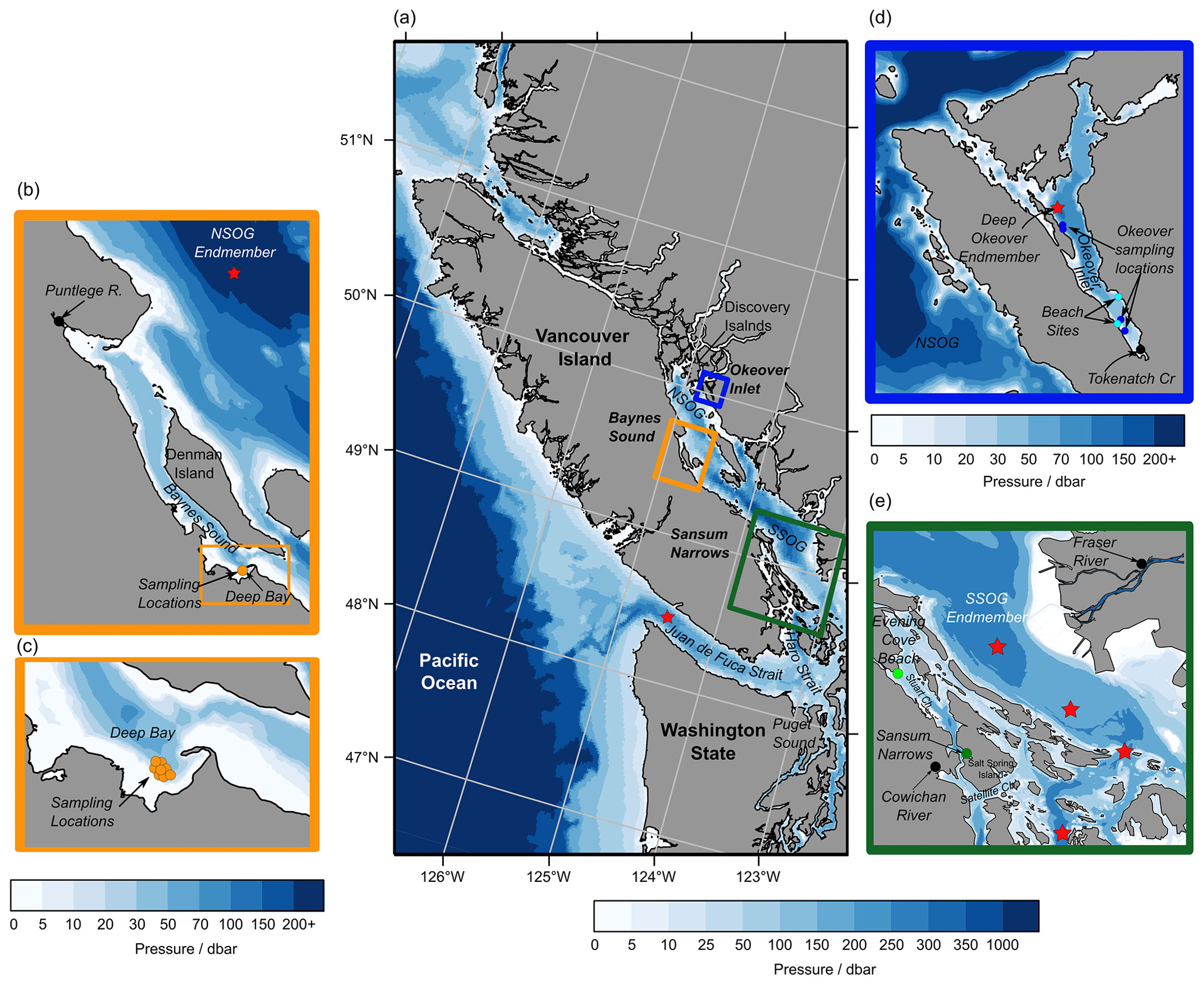
Figure 1 (a) Sampling sub-regions in the Salish Sea: Baynes Sound (orange), Okeover Inlet (blue), and Sansum Narrows (green). Multiple nearshore sites at shellfish leases were sampled in each sub-region as well as freshwater endmembers (black) and sub-surface salty endmembers (red stars) (b–e) (Tables A1 and A2 in the Appendix). (b) Baynes Sound, showing nearshore sampling locations in Deep Bay (orange), the Puntledge River freshwater endmember (black), and NSOG salty endmember (red star). (c) Deep Bay nearshore sampling locations at a tray hang lease. (d) Okeover Inlet, showing nearshore sampling locations taken at tray hang shellfish leases (dark blue) and beach grow sites (light blue), the freshwater endmember – Tokenatch creek – (black), and the deep-water salty endmember (red star). (e) Sansum Narrows showing nearshore shellfish lease sampling location (dark green) and beach grow site “Evening Cove beach” (light green) in Stuart Channel, the Cowichan River freshwater endmember for this region, and the Fraser River freshwater endmember for the SOG region (black) and the four stations that were used to determine the SSOG salty endmember (red stars). Credit: NE Pacific bathymetry from NOAA (2009), shorelines from NOAA (2017), and Baynes Sound bathymetry from Natural Resources Canada (2021).

2.2 Data collection and sample analysis

We collected discrete water samples from the Salish Sea for analysis of dissolved inorganic carbon (DIC), total alkalinity (TA), salinity (S), dissolved oxygen (DO), and nutrients (silicic acid, nitrate, and phosphate) over 20 campaigns spanning all seasons from 2015–2018. We sampled nearshore locations in Okeover Inlet, Baynes Sound, Sansum Narrows, and Evening Cove beach (Fig. 1). Sample locations were mostly active shellfish grow sites, including beach grow sites and tray hangings. Due to the strong stratification of our study system, Niskin bottles were used to collect samples from the surface layer (0 to 5 m), within the mid-depth layer (5 to 20 m) and near the bottom (away from beaches depth varied by location ∼ 30 to 100 m). Niskin bottles were deployed from small skiffs or at beaches where they were triggered by hand after wading in from shore. Conductivity, temperature, and depth (CTD) profiles were taken simultaneously in the water column using both a Castaway^® and RBR Concerto^® CTD (Simpson et al., 2022). We sampled throughout the day at most locations, starting in the morning (∼ 07:00 to 08:00 Pacific time) and concluding mid-afternoon (∼ 16:00 to 17:00). We took samples at least once during ebb, slack, and neap tides. No night-time samples were collected, assuming that the morning samples contained the maximum diel respiration signal. Sample collection and analysis followed standard procedures (Barwell-Clarke and Whitney, 1996; Carpenter, 1965; Dickson et al., 2007, and Culberson, 1991; see Simpson et al., 2022, Sect. A2 in the Appendix, for sample analysis detail).

Understanding the variability within these estuarine systems requires that we first characterize the waters that are entering and mixing from both freshwater and salty sources at each location. Thus, we characterized the freshwater and salty-water endmembers at each location. We collected discrete samples of DIC, TA, S, DO, and nutrients as well as CTD readings from local freshwater sources and from locations that are representative of the salty water that mixes into each study location (Table A1). Endmembers were selected based on the fit of observational data collected in the region to endmember salinity gradients (i.e., how well observational data fit the mixing line between fresh and salty endmembers) for Baynes Sound and Okeover Inlet (Simpson et al., 2022) and in Sansum Narrows and Evening Cove beach (Sect. A1).

To calculate pH, Ω_a, and Ω_c, we used the observed DIC, TA, silicic acid, phosphate, bottle salinities, and CTD temperature, and pressure to solve the carbonate system (full details in Simpson et al., 2022) using CO2SYS (Orr et al., 2018; van Heuven et al., 2011; Lewis and Wallace, 1998) with Millero (2010) carbonate constants (Millero, 2010), Dickson $K_{{\mathrm{SO}}_{\mathrm{4}}}$ constants (Dickson, 1990), Dickson and Riley K_F constants (Dickson and Riley, 1979), and Uppström borate constants (Uppström, 1974). We report pH on the total scale. Data were divided into two seasons: a productive season capturing the regional phytoplankton blooms (April–September) subsequently referred to as “summer” and less productive season (October–March) referred to as “winter”. Salinity is reported on the practical salinity scale (PSS78), as a dimensionless value with no units.

2.3 Salinity normalization

Normalized DIC and TA were estimated following Friis et al. (2003) using regionally derived DIC–S and TA–S relationships for each study sub-region (Fig. 1) established from site-specific endmembers (Table A2) and the mean annual salinity (${\stackrel{\mathrm{‾}}{S}}_{\mathrm{annual}}$), not weighted by season, at the location and depth range of interest (Table A3). Where available, the freshwater intercept for each DIC–S and TA–S relationship was determined directly from observations; where no freshwater data were available, we extrapolated to S=0 using the salinity relationship established for that location from the data available (Simpson et al., 2022). Normalizing DIC and TA to ${\stackrel{\mathrm{‾}}{S}}_{\mathrm{annual}}$ (${\mathrm{DIC}}_{\stackrel{\mathrm{‾}}{\mathrm{s}}}$ and ${\mathrm{TA}}_{\stackrel{\mathrm{‾}}{\mathrm{s}}}$) removes changes in these parameters resulting from dilution. In this region, the remaining variability can be attributed to biological processes (Simpson et al., 2022). We calculate the difference between the winter and summer mean ${\mathrm{DIC}}_{\stackrel{\mathrm{‾}}{\mathrm{s}}}$ and ${\mathrm{TA}}_{\stackrel{\mathrm{‾}}{\mathrm{s}}}$, to give the seasonal difference in DIC ($\mathrm{\Delta }{\mathrm{DIC}}_{\stackrel{\mathrm{‾}}{\mathrm{s}}}$) and TA ($\mathrm{\Delta }{\mathrm{TA}}_{\stackrel{\mathrm{‾}}{\mathrm{s}}}$) resulting from biological processes.

2.4 Drivers of seasonal change in pH and CaCO₃ saturation state

We estimate the individual contributions of biological processes, temperature, and freshwater to seasonal changes in pH, Ω_a, and Ω_c (ΔpH, ΔΩ_a, and ΔΩ_c) at each location and depth, using a first-order Taylor expansion (e.g., Sarmiento and Gruber, 2006; Lovenduski et al., 2007; Turi et al., 2016; Franco et al., 2021) (Eqs. 1–3):

$$\begin{array}{}\text{(1)}& {\displaystyle }\begin{array}{rl}\mathrm{\Delta }\mathrm{pH}& \approx {\displaystyle \frac{\partial \mathrm{pH}}{\partial \mathrm{DIC}}}\mathrm{\Delta }{\mathrm{DIC}}_{\stackrel{\mathrm{‾}}{\mathrm{s}}}+{\displaystyle \frac{\partial \mathrm{pH}}{\partial \mathrm{TA}}}\mathrm{\Delta }{\mathrm{TA}}_{\stackrel{\mathrm{‾}}{\mathrm{s}}}+{\displaystyle \frac{\partial \mathrm{pH}}{\partial T}}\mathrm{\Delta }T\\ & +{\displaystyle \frac{\partial \mathrm{pH}}{\partial \mathrm{fw}}}\mathrm{\Delta }\mathrm{fw}\end{array}\text{(2)}& {\displaystyle }\begin{array}{rl}\mathrm{\Delta }{\mathrm{\Omega }}_{\mathrm{a}}& \approx {\displaystyle \frac{\partial {\mathrm{\Omega }}_{\mathrm{a}}}{\partial \mathrm{DIC}}}\mathrm{\Delta }{\mathrm{DIC}}_{\stackrel{\mathrm{‾}}{\mathrm{s}}}+{\displaystyle \frac{\partial {\mathrm{\Omega }}_{\mathrm{a}}}{\partial \mathrm{TA}}}\mathrm{\Delta }{\mathrm{TA}}_{\stackrel{\mathrm{‾}}{\mathrm{s}}}+{\displaystyle \frac{\partial {\mathrm{\Omega }}_{\mathrm{a}}}{\partial T}}\mathrm{\Delta }T\\ & +{\displaystyle \frac{\partial {\mathrm{\Omega }}_{\mathrm{a}}}{\partial \mathrm{fw}}}\mathrm{\Delta }\mathrm{fw}\end{array}\text{(3)}& {\displaystyle }\begin{array}{rl}\mathrm{\Delta }{\mathrm{\Omega }}_{\mathrm{c}}& \approx {\displaystyle \frac{\partial {\mathrm{\Omega }}_{\mathrm{c}}}{\partial \mathrm{DIC}}}\mathrm{\Delta }{\mathrm{DIC}}_{\stackrel{\mathrm{‾}}{\mathrm{s}}}+{\displaystyle \frac{\partial {\mathrm{\Omega }}_{\mathrm{c}}}{\partial \mathrm{TA}}}\mathrm{\Delta }{\mathrm{TA}}_{\stackrel{\mathrm{‾}}{\mathrm{s}}}+{\displaystyle \frac{\partial {\mathrm{\Omega }}_{\mathrm{c}}}{\partial T}}\mathrm{\Delta }T\\ & +{\displaystyle \frac{\partial {\mathrm{\Omega }}_{\mathrm{c}}}{\partial \mathrm{fw}}}\mathrm{\Delta }\mathrm{fw}.\end{array}\end{array}$$

The first and second terms on the right-hand side of Eqs. (1)–(3) represent the contribution of biologically driven changes in DIC and TA, to ΔpH, ΔΩ_a, and ΔΩ_c, respectively. The third term is the contribution of seasonal temperature difference (ΔT), the difference between mean winter and mean summer T, to ΔpH, ΔΩ_a, or ΔΩ_c. The final term is the freshwater component (fw), defined in Eqs. (4)–(6).

Partial derivatives provide a measure of the sensitivity of pH and Ω to a small change in one environmental variable when all other carbonate system parameters (i.e., TA, T, and S) are held constant. For example, the partial derivatives $\frac{\partial \mathrm{pH}}{\partial \mathrm{DIC}}$, $\frac{\partial {\mathrm{\Omega }}_{\mathrm{a}}}{\partial \mathrm{DIC}}$, and $\frac{\partial {\mathrm{\Omega }}_{\mathrm{c}}}{\partial \mathrm{DIC}}$ in Eqs. (1)–(3) measure how much pH, Ω_a, and Ω_c respond to a small change in DIC. We calculate partial derivatives of Ω_a and Ω_c (Table A4) using the derivnum function in CO2SYS (Orr et al., 2018). At the time of writing, there was no function in derivnum to calculate partial derivatives of pH. We calculated the partial derivatives of pH using the same finite step sizes used in derivnum to calculate partial derivatives of Ω_a and Ω_c and re-solved the system using CO2SYS (Sect. A2).

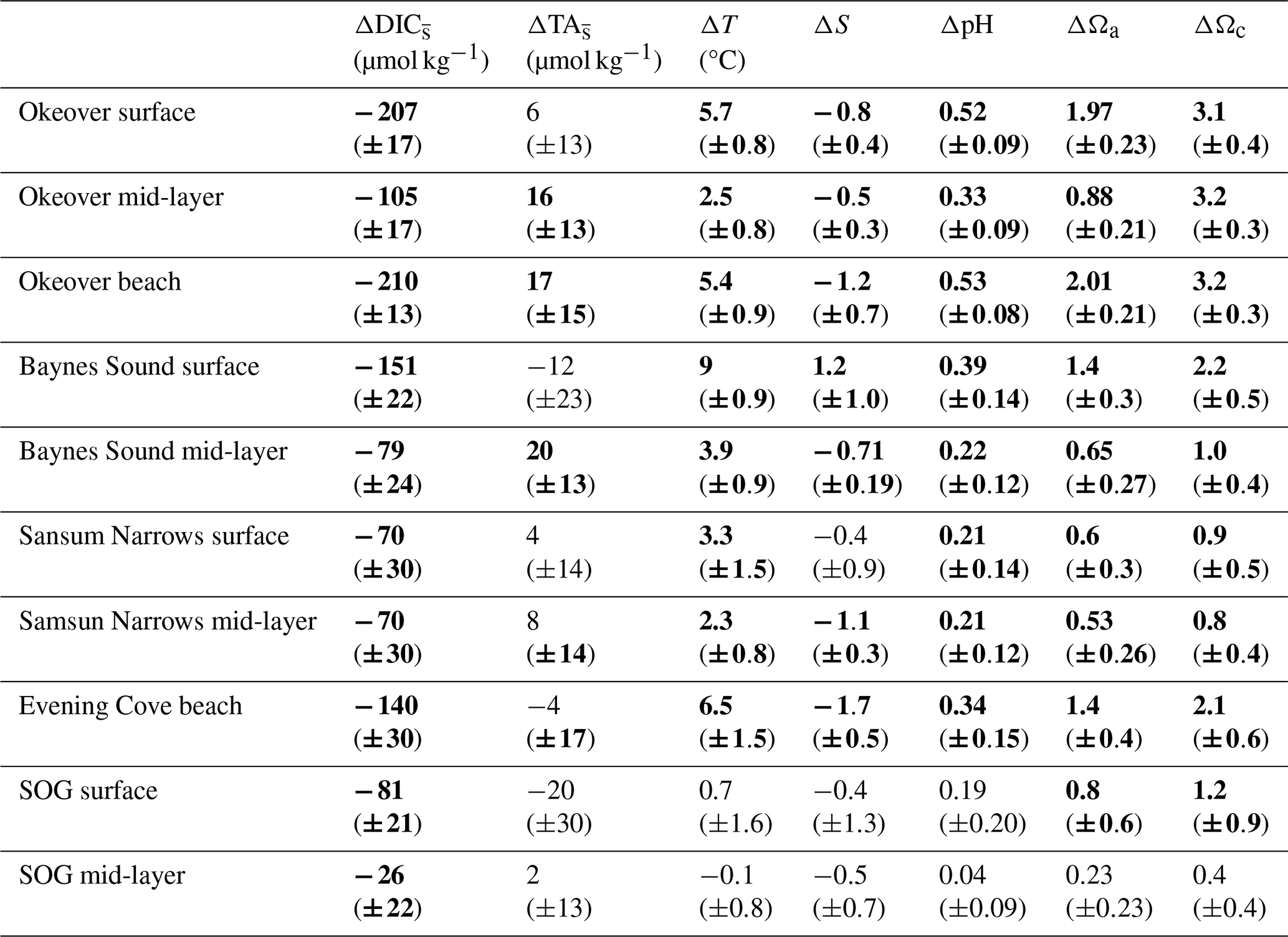
To calculate the total seasonal ΔpH, ΔΩ_a, and ΔΩ_c, we multiply partial derivatives with the observed seasonal changes in each individual driver, i.e., biologically driven DIC ($\mathrm{\Delta }{\mathrm{DIC}}_{\stackrel{\mathrm{‾}}{\mathrm{s}}}$), biologically driven TA ($\mathrm{\Delta }{\mathrm{TA}}_{\stackrel{\mathrm{‾}}{\mathrm{s}}}$), seasonal temperature change (ΔT), and seasonal freshwater contribution (Δfw). The seasonal differences in DIC and TA are normalized to the annual mean salinity (Table 1).

The contribution of seasonal changes in freshwater to ΔpH, ΔΩ_a, or ΔΩ_c is defined as

$$\begin{array}{}\text{(4)}& {\displaystyle \frac{\partial \mathrm{pH}}{\partial \mathrm{fw}}}\mathrm{\Delta }\mathrm{fw}\approx {\displaystyle \frac{\partial \mathrm{pH}}{\partial S}}\mathrm{\Delta }S+{\displaystyle \frac{\partial \mathrm{pH}}{\partial \mathrm{TA}}}\mathrm{\Delta }{\mathrm{TA}}_{\mathrm{fw}}+{\displaystyle \frac{\partial \mathrm{pH}}{\partial \mathrm{DIC}}}\mathrm{\Delta }{\mathrm{DIC}}_{\mathrm{fw}}\text{(5)}& {\displaystyle \frac{\partial {\mathrm{\Omega }}_{\mathrm{a}}}{\partial \mathrm{fw}}}\mathrm{\Delta }\mathrm{fw}\approx {\displaystyle \frac{\partial {\mathrm{\Omega }}_{\mathrm{a}}}{\partial S}}\mathrm{\Delta }S+{\displaystyle \frac{\partial {\mathrm{\Omega }}_{\mathrm{a}}}{\partial \mathrm{TA}}}\mathrm{\Delta }{\mathrm{TA}}_{\mathrm{fw}}+{\displaystyle \frac{\partial {\mathrm{\Omega }}_{\mathrm{a}}}{\partial \mathrm{DIC}}}\mathrm{\Delta }{\mathrm{DIC}}_{\mathrm{fw}}\text{(6)}& {\displaystyle \frac{\partial {\mathrm{\Omega }}_{\mathrm{c}}}{\partial \mathrm{fw}}}\mathrm{\Delta }\mathrm{fw}{\displaystyle \frac{\partial \mathrm{\Omega }\mathrm{c}}{\partial S}}\mathrm{\Delta }S+{\displaystyle \frac{\partial {\mathrm{\Omega }}_{\mathrm{c}}}{\partial \mathrm{TA}}}\mathrm{\Delta }{\mathrm{TA}}_{\mathrm{fw}}+{\displaystyle \frac{\partial {\mathrm{\Omega }}_{\mathrm{c}}}{\partial \mathrm{DIC}}}\mathrm{\Delta }{\mathrm{DIC}}_{\mathrm{fw}}.\end{array}$$

The first term on the right-hand side of Eqs. (4)–(6) is the contribution of seasonal S differences (ΔS) to seasonal ΔpH, ΔΩ_a, and ΔΩ_c, arising from the salinity dependence of carbonate system constants (e.g., Millero et al., 2006), where ΔS is the difference between mean winter S (${\stackrel{\mathrm{‾}}{S}}_{\mathrm{winter}}$) and mean summer S (${\stackrel{\mathrm{‾}}{S}}_{\mathrm{summer}}$). The final two terms, ΔDIC_fw and ΔTA_fw, in Eqs. (4)–(6), represent the change in DIC and TA driven by seasonal salinity change (ΔS), or in other words, dilution. To calculate ΔDIC_fw and ΔTA_fw, we used regionally specific DIC–S and TA–S relationships to estimate the change in DIC and TA along the salinity gradient resulting from salinity change with freshwater input (ΔS). We estimate uncertainty in the Taylor expansion results from both derivative and seasonal change uncertainties (Sect. A3). The unusual coccolithophore bloom that occurred in Okeover in 2016 (NASA, 2016) has been excluded from the seasonal analysis, as it was an anomalous event spanning a shorter temporal scale, lasting days to weeks. It is, however, included in the diel analysis.

2.5 Diel drivers of pH and CaCO₃ saturation state

We also investigate the drivers of diel variability at locations where sufficient observations were made during both the morning and afternoon to capture changes in carbonate chemistry throughout the day. Specifically, we required sampling over a minimum of 6 h, capturing morning, noon, and afternoon at a given day and location. We selected a day from both the summer and winter season at each site for analysis (Table 2). When multiple days fulfilled this requirement at a particular location, we analyzed the day that had the greatest range in conditions or drivers of pH and Ω. The winter day chosen for Baynes Sound was selected due to a large range in salinity observed throughout the day. While a large winter diel salinity range is not necessarily representative of everyday conditions in Baynes Sound, we chose the day with the greatest range to investigate the importance of freshwater as a potential diel driver of carbonate chemistry conditions. In the Okeover region, the only data meeting our diel criteria were collected at the beach location in summer, during the unusual coccolithophore bloom that occurred in 2016 (NASA, 2016; Simpson et al., 2022).

We estimate the diel contribution of drivers of pH, Ω_a, and Ω_c variability in the surface layer only (0 to 5 m), as we sampled the surface layer more frequently and captured samples from the same location throughout the day. We estimate the diel drivers using Eqs. (1)–(6), using the same partial derivatives calculated for the seasonal Taylor analysis (Table A4), but here we use the difference in DIC, TA, T, and S observed over a single day (Table 2) rather than season. We estimate the biologically driven diel ΔDIC and ΔTA in Eqs. (1)–(3), using the change in ${\mathrm{DIC}}_{\stackrel{\mathrm{‾}}{\mathrm{s}}}$ and ${\mathrm{TA}}_{\stackrel{\mathrm{‾}}{\mathrm{s}}}$ over the day. The freshwater component (Eqs. 4–6) was estimated using the DIC–S and TA–S relationships calculated for each location (as above), with the observed diel range in salinity (ΔS). ${\mathrm{DIC}}_{\stackrel{\mathrm{‾}}{\mathrm{s}}}$ and ${\mathrm{TA}}_{\stackrel{\mathrm{‾}}{\mathrm{s}}}$ were normalized to ${\stackrel{\mathrm{‾}}{S}}_{\mathrm{annual}}$, for the depth and location of interest as above, following Friis et al. (2003) (Sect. 2.2). We keep the salinity normalization the same for the diel and seasonal analysis (i.e., rather than normalizing to a seasonal salinity) to avoid shifting to a point in carbonate space with different sensitivity (e.g., Egleston et al., 2010; Hu and Cai, 2013; Simpson et al., 2022). Thus, results from the seasonal and diel Taylor analyses, as well as the winter and summer diel analyses, may be directly compared.

3 Results

3.1 Seasonal variability

At each nearshore location, variability in both chemical and physical properties around the median (Figs. 2 and 3) is particularly strong at the surface and in summer. The open-water SOG region also has high variability in summer as it covers a large geographical extent including both the distinct NSOG and SSOG basins, which includes the Fraser River plume. However, the open-water SOG has lower median pH and Ω than the nearshore in summer and slightly higher pH and Ω in winter. If we assume that our diverse sites (including beaches and tidal channels, Fig. 1) are representative of the nearshore environment of the Salish Sea region, the nearshore experiences greater variability than the open waters of the SOG in both winter and summer. Okeover Inlet, in particular, has high pH and Ω that contribute substantially to the larger range in carbonate chemistry conditions in the nearshore.

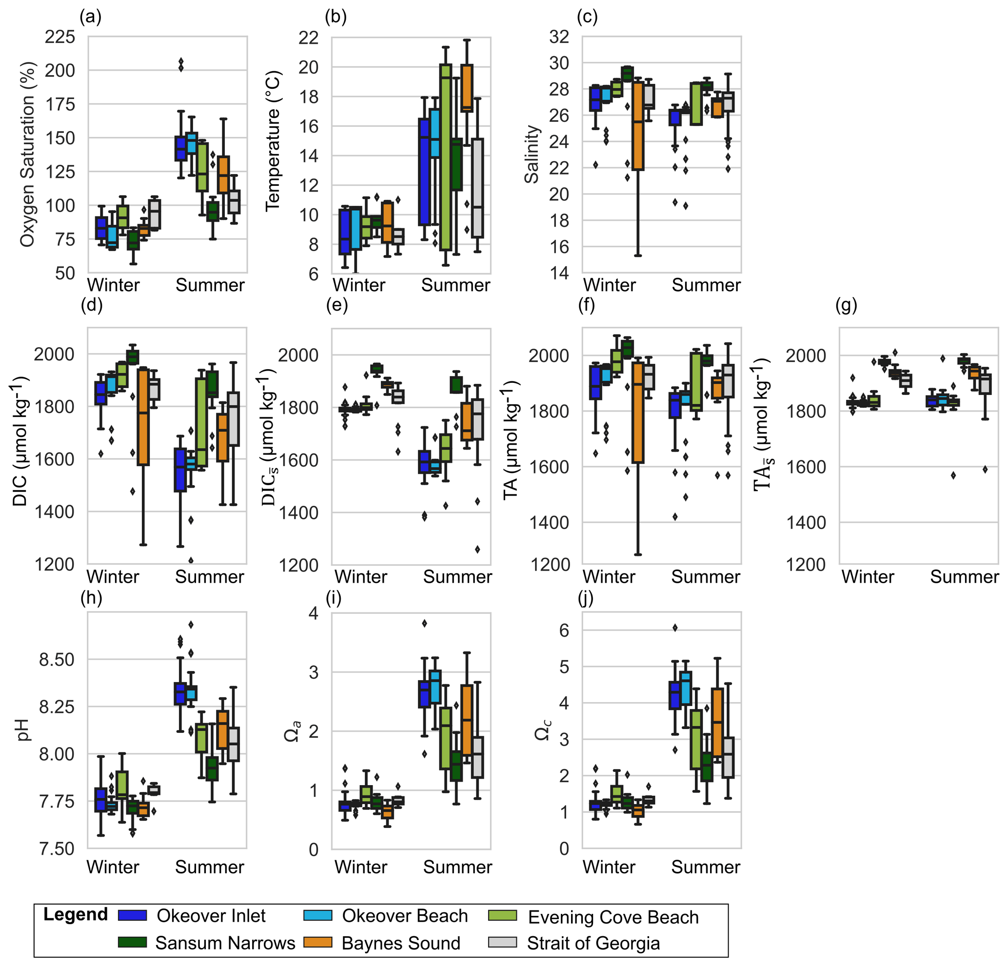
Figure 2 Observed variability at shellfish grow sites and adjacent waters in the surface layer (0–5 m) in winter and summer, respectively in (a) dissolved oxygen (% saturation), (b) temperature, (c) salinity, (d) dissolved inorganic carbon (DIC), (e) salinity-normalized DIC (${\mathrm{DIC}}_{\stackrel{\mathrm{‾}}{\mathrm{s}}}$), (f) total alkalinity (TA), (g) salinity-normalized TA (${\mathrm{TA}}_{\stackrel{\mathrm{‾}}{\mathrm{s}}}$), (h) pH, (i) Ω_a, and (j) Ω_c at nearshore locations shown in Fig. 1: Okeover (dark blue), Okeover beach (light blue), Evening Cove beach (light green), Sansum Narrows (dark green), Baynes Sound (orange), and ship collected data from the SOG (grey). Data have been split into a summer season capturing phytoplankton blooms (April–September) and winter season (October–March) when productivity is low. The mean annual salinity (Table A3) at each location was used to normalize DIC and TA, to show the impact of dilution. There is inter-seasonal variability at all locations and generally greater variability and range of conditions during the summer season, with the exception of salinity during the winter season in Baynes Sound. Boxes represent the interquartile range in conditions, middle bars are the median value and outer bars the full range in values, and points are outliers. The number of samples used to generate plots is given in Table A8.

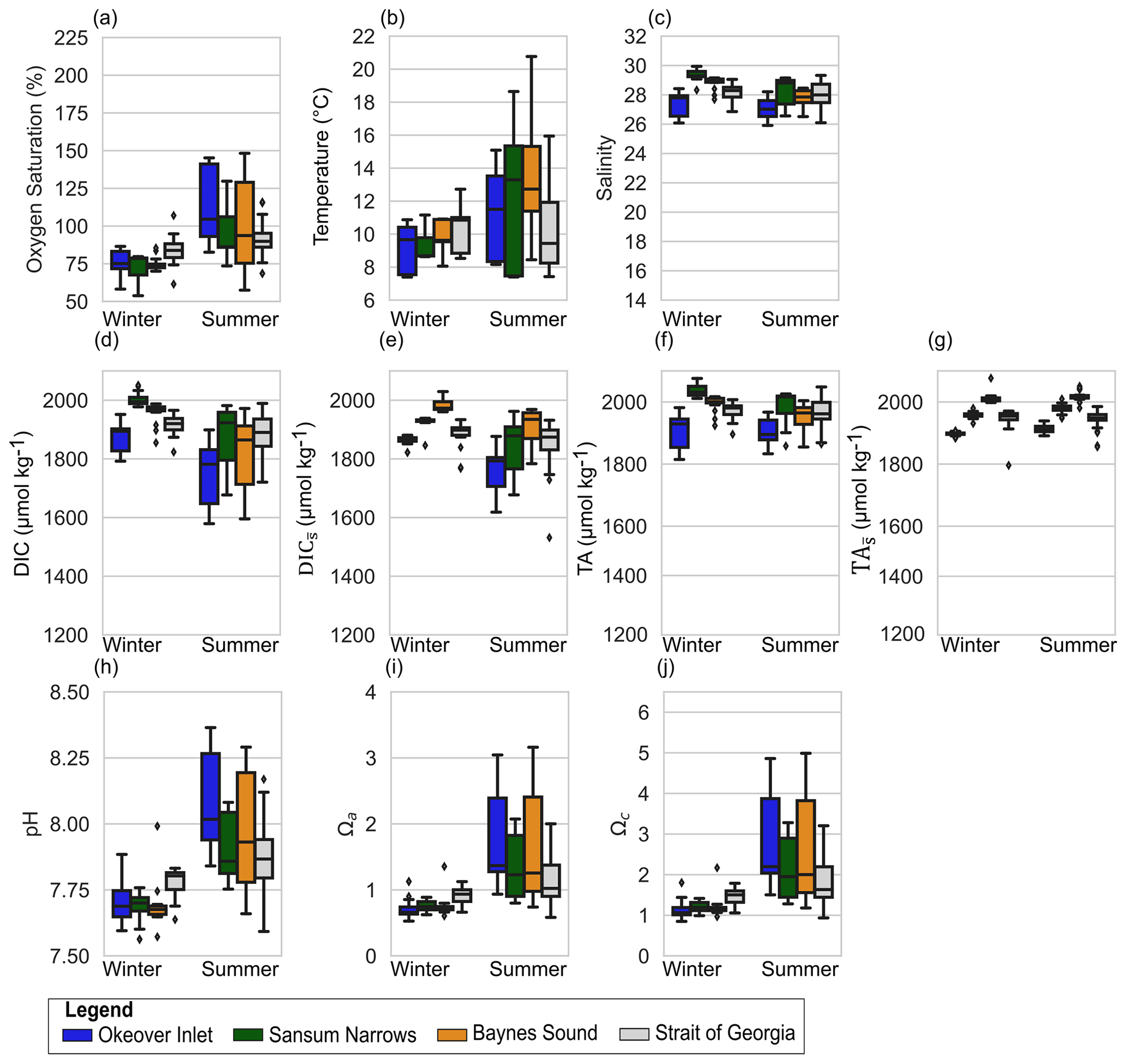
Figure 3 Observed variability in the 5–20 m layer at shellfish grow sites and in adjacent waters in (a) dissolved oxygen (% saturation), (b) temperature, (c) salinity, (d) dissolved inorganic carbon (DIC), (e) salinity-normalized DIC (${\mathrm{DIC}}_{\stackrel{\mathrm{‾}}{\mathrm{s}}}$), (f) total alkalinity (TA), (g) salinity-normalized TA (${\mathrm{TA}}_{\stackrel{\mathrm{‾}}{\mathrm{s}}}$), (h) pH, (i) Ω_a, and (j) Ω_c at nearshore locations shown in Fig. 1: Okeover (dark blue), Sansum Narrows (dark green), Baynes Sound (orange), and ship collected data from the SOG (grey). Data have been split into a summer season capturing the phytoplankton bloom (April–September) and winter season (October–March). Note that y axes are the same as Fig. 2 for comparison, and locations by season are shown in the same order right to left in each panel. The mean annual salinity (Table A3) at each location was used to normalize DIC and TA to show the impact of dilution. Similar to the surface layer, there is inter-seasonal variability at all locations and greater variability and range of conditions during the summer season. There is lower variability in conditions in the mid-layer than in the surface. Boxes represent the interquartile range in conditions, middle bars are the median value, outer bars the full range in values, and points are outliers. The number of samples used to generate plots is given in Table A8.

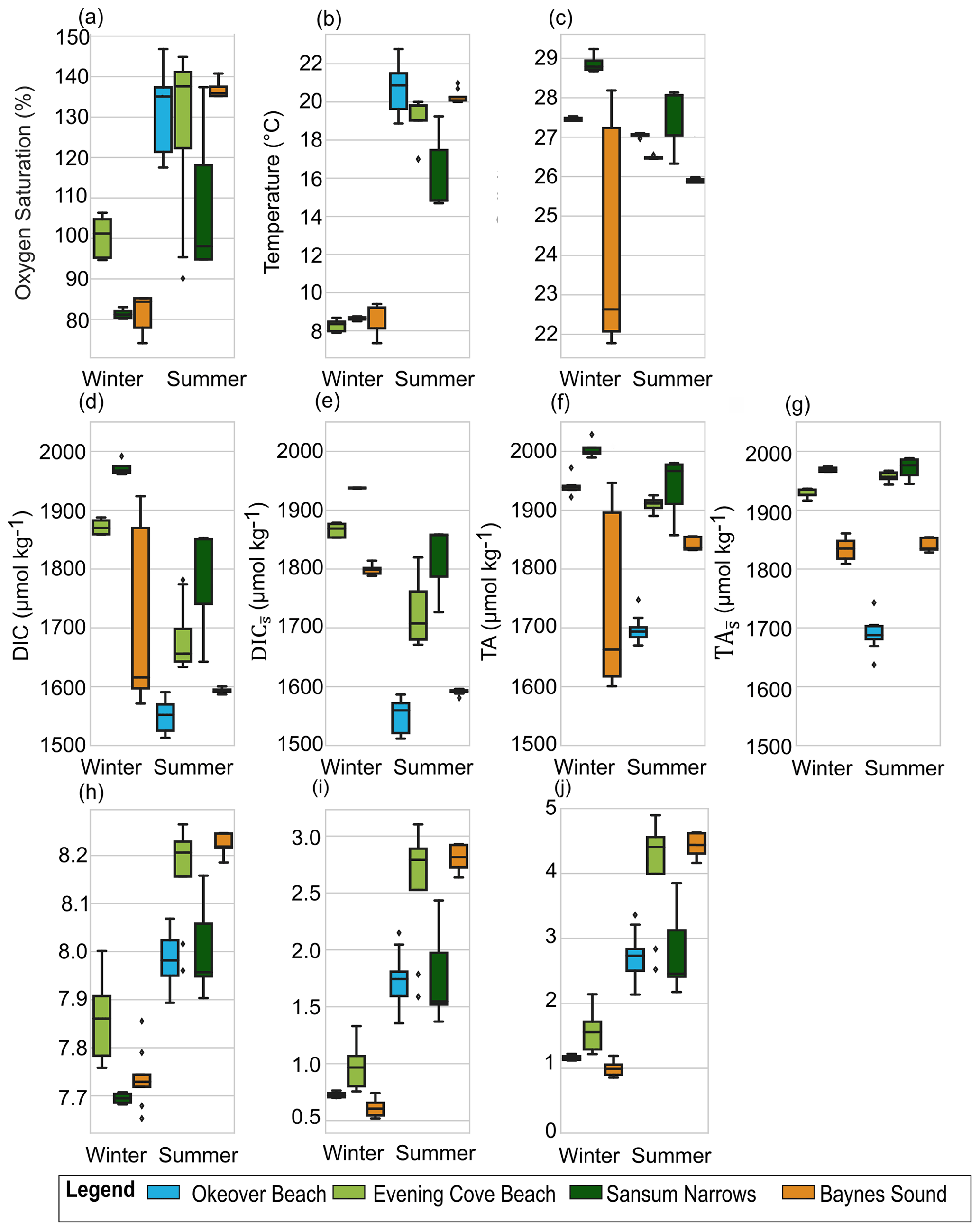
Figure 4 Variability in the surface layer (0 to 5 m) during one sampling day (Table 2) at Baynes Sound (orange), Evening Cove beach (light green), and Sansum Narrows (dark green) for both summer and winter, and Okeover beach (light blue) in summer only, in (a) dissolved oxygen (% saturation), (b) temperature, (c) salinity, (d) dissolved inorganic carbon (DIC), (e) salinity-normalized DIC (${\mathrm{DIC}}_{\stackrel{\mathrm{‾}}{\mathrm{s}}}$), (f) total alkalinity (TA), (g) salinity-normalized TA (${\mathbf{TA}}_{\stackrel{\mathrm{‾}}{\mathrm{s}}})$, (h) pH, (i) Ω_a, and (j) Ω_c in winter (left) and summer (right). The mean annual salinity (Table A3) at each location was used to normalize DIC and TA (e, h) to show the impact of dilution. Boxes represent the interquartile range in conditions, middle bars are the median value, outer bars the full range in values, and points are outliers. y axes are different to Figs. 2 and 3 above.

3.1.1 Temperature

Surface temperatures (T) experience modest variability across all locations in winter, ranging from ∼ 6 to 11 °C, with similar median T ∼ 9 °C across sites (Fig. 2b). The lowest surface T variability of the nearshore locations is found in Sansum Narrows where tidal mixing is strong. Winter mid-layer temperatures are warmer than the surface (∼ 1 °C) and exhibit lower variability (Fig. 3b). Summer surface temperatures are higher (median ∼ 15 to 19 °C), reaching up to 22 °C in Baynes Sound and Evening Cove beach. Summer temperatures are also more variable than in winter, with particularly large ranges in surface temperatures at Evening Cove beach and Sansum Narrows (Fig. 2b). In our observations, Baynes Sound surface temperatures are the highest, and we observe cooler summer temperatures in Okeover Inlet, with one exception – the unusual conditions that occurred during the 2016 coccolithophore bloom (NASA, 2016), when summer temperatures were unusually high (up to 22 °C). Although summer surface temperatures exhibit a similar range in the SOG and nearshore sites, median summer surface temperatures in the SOG are cooler than in the nearshore in our observations. Summer mid-layer variability is lower than surface variability, ranging from 8 to 20 °C, and mid-layer temperatures are ∼ 4 °C cooler than surface temperatures.

3.1.2 Salinity

Each nearshore location has a distinct salinity (S) median and range (Fig. 2c). The SOG and our nearshore sites are relatively fresh, and in our observations, the lowest median surface winter salinities (∼ 25) are found in Baynes Sound. The highest median winter salinities are found where tidal mixing is strong, Sansum Narrows (∼ 29), which is higher than the median salinity of the SOG (∼ 27). The most prominent surface salinity variability (ranging from 15 to 29) is seen in Baynes Sound during winter, where we observed strong stratification with a lower salinity brackish lens on several occasions. Winter surface variability across the remaining nearshore locations is moderate (ranging by ∼ 2), with a greater range in salinity in the nearshore than in the SOG.

There is little salinity variability between seasons at all sites, indicating a balance between winter pluvial, and summer glacial freshwater inputs. Surface salinity ranges are also similar in both seasons, except for Baynes Sound, which exhibits a large salinity range in winter but not in summer in our data. Okeover is fresher than any other nearshore location in summer. Nearshore salinity ranges are similar to the SOG region in summer, likely due to lower salinities in the SSOG in summer (<25) attributed to the Fraser River freshet. Mid-layer salinities in the nearshore are higher than the surface and similar in winter and summer, although summer appears marginally fresher (Fig. 3c). The exception is the tidally mixed Sansum Narrows, where salinities are similar in both the surface and mid-layer.

3.1.3 DIC and TA

Surface median DIC and TA are higher in winter than in summer at all sites, although this seasonal difference is minimal in Sansum Narrows and even smaller in the SOG (Fig. 2d and f). Sansum Narrows has the highest winter median DIC and TA of all locations, including the SOG. Winter surface DIC and TA ranges are low and are similar across sites (∼ 100 to 200 µmol kg⁻¹), except for in Baynes Sound where DIC and TA exhibit a large range of ∼ 700 µmol kg⁻¹. Winter DIC and TA at our locations are highly salinity dependent (Simpson et al., 2022), as demonstrated by medians and ranges (Fig. 2d, f) following a similar pattern to salinity (Fig. 2c). The large winter range in DIC and TA observed in Baynes Sound is a result of the exceptional salinity range observed at this location. Summer surface DIC and TA are low in the nearshore (Fig. 2d, f) and are generally lower than in the SOG, particularly in Okeover Inlet. The ranges in DIC at nearshore sites in summer are larger than winter, except for Baynes Sound, where a larger, salinity-driven range in DIC and TA occurs in winter.

Following salinity, median mid-layer TA values are higher than in the surface layer (by ∼ 40 to 50 µmol kg⁻¹), in both winter and summer (Fig. 3d and f). Winter mid-layer DIC is also ∼ 40 to 50 µmol kg⁻¹ higher than the surface, but in summer mid-layer DIC is much higher than the surface (by 150 to 220 µmol kg⁻¹), especially in Baynes Sound and Okeover Inlet. In the tidally mixed Sansum Narrows, this DIC difference is less (∼ 80 µmol kg⁻¹). Variability in mid-layer DIC and TA in winter is similar to the variability seen in the surface layer (except in Baynes Sound where surface dilution is strong). Summer variability in the mid-layer is greater than in winter, similar across nearshore sites (a range of ∼ 300 µmol kg⁻¹), and far less than the variability observed in the surface.

When DIC and TA are normalized (${\mathrm{DIC}}_{\stackrel{\mathrm{‾}}{\mathrm{s}}}$, ${\mathrm{TA}}_{\stackrel{\mathrm{‾}}{\mathrm{s}}}$, respectively) to the annual mean salinity by sub-region (Sect. 2.3), their ranges shrink, especially in winter (Figs. 2e, g; 3e, g). However, the range in summer ${\mathrm{DIC}}_{\stackrel{\mathrm{‾}}{\mathrm{s}}}$ remains relatively large, when other processes, such as primary production, illustrated by high levels of dissolved oxygen, contribute to variability throughout the surface and into the mid-layer. The small ranges in the salinity-normalized quantities indicate the predominant salinity dependence (e.g., Simpson et al., 2022).

3.1.4 Dissolved oxygen

Winter surface dissolved oxygen (DO; expressed as % saturation) is mostly undersaturated (i.e., <100 %, with medians ∼ 75 %–85 %) at our nearshore locations, and variability is low across sites (Fig. 2a). Sansum Narrows has relatively low DO compared to the other nearshore locations. Mid-layer winter DO is lower than in the surface layer (<80 %) (Fig. 3a). In summer, surface DO is mostly supersaturated, with high DO and large variability, especially in Okeover Inlet. However, the well-mixed Sansum Narrows location has the lowest DO, which is mostly undersaturated (Figs. 2a, 3a). Mid-layer DO in summer is also higher than it is in winter. At times this depth zone includes a strong oxycline and ranges from supersaturation to undersaturation (although still oxygen replete, lowest DO usually >70 % saturation, Fig. A1 in the Appendix and Fig. 3a). Ranges of DO in the SOG are similar to those in the nearshore in winter but are lower in summer (Figs. 2a, 3a).

3.1.5 pH

Winter surface pH values at nearshore sites are lower than in summer, ranging from ∼ 7.6 to 8.1 across all locations (Fig. 2h). Winter surface pH is similar at all nearshore locations and is lower than the SOG region. Largest ranges in surface pH are found in Okeover Inlet and at Evening Cove beach (∼ 0.5), and these ranges are similar in both winter and in summer. However, in Baynes Sound and Sansum Narrows winter surface pH variability is lower than summer variability. In winter, when productivity is low, the surface and mid-layer experience similar pH. Variability is lower in the mid-layer, especially so at Sansum Narrows and Baynes Sound (Fig. 3h).

Summer median pH is relatively high, especially in Okeover Inlet (surface ∼ 8.3; Fig. 2h). Okeover Inlet also experiences the highest summer pH of the nearshore locations, reaching a maximum pH of ∼ 8.6 within the inlet and ∼ 8.7 at the beach. Sansum Narrows has the lowest summer surface pH of ∼ 7.85, comparable to winter conditions at other nearshore locations. Typically, lower pH at nearshore locations corresponds with higher DIC (Fig. 2d). Interestingly, however, the large DIC range seen in Baynes Sound in winter does not result in a similarly large range in pH. TA also shifts with salinity in winter, and at this location the DIC : TA ratio remains nearly constant along the salinity gradient (Fig. 4 in Simpson et al., 2022), which keeps pH similar. Like oxygen saturation, summer mid-layer pH variability is similar to the range found in the surface. Generally, mid-layer pH is much lower than in the surface layer, when conditions are stratified, and the surface is productive. In contrast, where mixing is strong, median summer mid-layer pH is about the same as surface pH, e.g., in Sansum Narrows. Sansum Narrows also has the lowest summer median mid-layer pH of the nearshore sites of 7.8.

Nearshore pH ranges in both the surface and mid-layers are smaller than those found in the SOG region. However, when considering all nearshore sites collectively as the nearshore, the total range in pH is 7.75 to 8.6, making summer surface pH variability at the nearshore significantly larger than open-water variability.

3.1.6 Aragonite and calcite saturation states – Ω_a and Ω_c

Surface Ω_a and Ω_c follow a similar variability pattern, although their absolute values differ (i.e., Ω_c is greater; Fig. 2i, j). Winter surface and mid-layer Ω are lower than summer surface Ω. Almost all locations, nearshore and the SOG, are undersaturated throughout the water column with respect to Ω_a in winter (Fig. 2i), with only a few outlying samples that are supersaturated. While median winter surface Ω_c values are slightly greater than the saturation threshold (Ω_c=1), there is some Ω_c undersaturation in our winter data at nearshore sites, particularly at Baynes Sound and Okeover Inlet (Fig. 2j), with the beach sites being the only nearshore locations to not experience any Ω_c undersaturation in our data. Median surface winter Ω_a is similar across all sites (∼ 0.8), and absolute variability is comparatively low relative to summer at all nearshore locations.

Summer Ω_a is high at our nearshore locations, which are mostly all supersaturated and reach values as high as 3.2 (Okeover and Baynes Sound). However, there is some summer surface undersaturation (Ω_a) in Sansum Narrows and in the SOG, where Ω values are typically lower (Fig. 2i, j). Ω_c is supersaturated at all locations, and values and variability are much higher than in winter (Fig. 2j), with maximum values reaching ∼ 4.5 to 5. High Ω_a in Okeover Inlet stands out from other nearshore locations, where the highest median Ω_a values are found at Okeover beach and Okeover Inlet (> 2.8, Fig. 2i). Following patterns in pH and oxygen, summer mid-layer Ω_a values are typically lower than in the surface, when the system is stratified and productive (and mid-layer summer saturation states in Sansum Narrows are similar to surface values). Variability in the mid-layer is similar to the surface, with variability being higher in Okeover Inlet and Baynes Sound, and lower in Sansum Narrows and the SOG.

3.2 Drivers of seasonal change in pH and Ω

Large changes in pH and Ω occur from winter to summer at all nearshore sites (Figs. 2 and 3, Table 1). The largest seasonal differences in pH and Ω are seen throughout Okeover Inlet, at beaches, and at the surface of Baynes Sound. Biologically driven changes in DIC ($\mathrm{\Delta }{\mathrm{DIC}}_{\stackrel{\mathrm{‾}}{\mathrm{s}}}$) contribute the most to seasonal change in pH and Ω, followed by seasonal ΔT (Fig. 5, Table A9). The temperature contribution to seasonal ΔpH is, however, much smaller than, and in the opposite direction to, the contribution of $\mathrm{\Delta }{\mathrm{DIC}}_{\stackrel{\mathrm{‾}}{\mathrm{s}}}$ (15 %–20 % of $\frac{\partial \mathrm{pH}}{\partial \mathrm{DIC}}\mathrm{\Delta }{\mathrm{DIC}}_{\stackrel{\mathrm{‾}}{\mathrm{s}}}$). The T contribution to seasonal change in Ω is negligible, 1–2 orders of magnitude less than the contribution of $\mathrm{\Delta }{\mathrm{DIC}}_{\stackrel{\mathrm{‾}}{\mathrm{s}}}$ and is within, or close to, uncertainty.

Values of $\mathrm{\Delta }{\mathrm{TA}}_{\stackrel{\mathrm{‾}}{\mathrm{s}}}$ are all within or close to measurement uncertainty (Table 1) indicating no, or minimal, biologically mediated TA flux. Regardless, we estimated the magnitude of pH change that these relatively small $\mathrm{\Delta }{\mathrm{TA}}_{\stackrel{\mathrm{‾}}{\mathrm{s}}}$ would drive. Once errors are propagated through the Taylor analysis (see Sect. A3 for methods), there are two instances where the contribution of biological TA to seasonal change in pH is just greater than uncertainty (Table A9). These ${\mathrm{TA}}_{\stackrel{\mathrm{‾}}{\mathrm{s}}}$ contributions to pH change drive a 0.05 (±0.04) and 0.07 (±0.05) increase in pH from winter to summer, in the mid-layer at Baynes Sound and Okeover, respectively.

These TA-driven increases in pH indicate that there could be a small biological uptake of TA from the water in winter and/or a small biological TA source in summer, both of which seem unlikely. For a biological source of TA to be present in summer, dissolution of CaCO₃ structures would need to occur during times of Ω_a and Ω_c supersaturation. Equally, a TA sink in winter is unlikely due to widespread and persistent low productivity. Changes in pH driven by in ${\mathrm{TA}}_{\stackrel{\mathrm{‾}}{\mathrm{s}}}$ are negligible in relation to the contributions of $\mathrm{\Delta }{\mathrm{DIC}}_{\stackrel{\mathrm{‾}}{\mathrm{s}}}$ and ΔT and are of the same order of magnitude as uncertainty. Changes in Ω_a and Ω_c driven by ${\mathrm{TA}}_{\stackrel{\mathrm{‾}}{\mathrm{s}}}$ are also low, close to uncertainty and negligible in relation to the contributions of $\mathrm{\Delta }{\mathrm{DIC}}_{\stackrel{\mathrm{‾}}{\mathrm{s}}}$ and ΔT.

The contributions of freshwater to seasonal changes in pH and Ω are also statistically negligible, as they are within or close to uncertainty, and any contribution outside of uncertainty is more than an order of magnitude less than the contribution from $\mathrm{\Delta }{\mathrm{DIC}}_{\stackrel{\mathrm{‾}}{\mathrm{s}}}$. Our results and discussion therefore focus on the contributions of $\mathrm{\Delta }{\mathrm{DIC}}_{\stackrel{\mathrm{‾}}{\mathrm{s}}}$ and ΔT to seasonal changes in pH, Ω_a, and Ω_c.

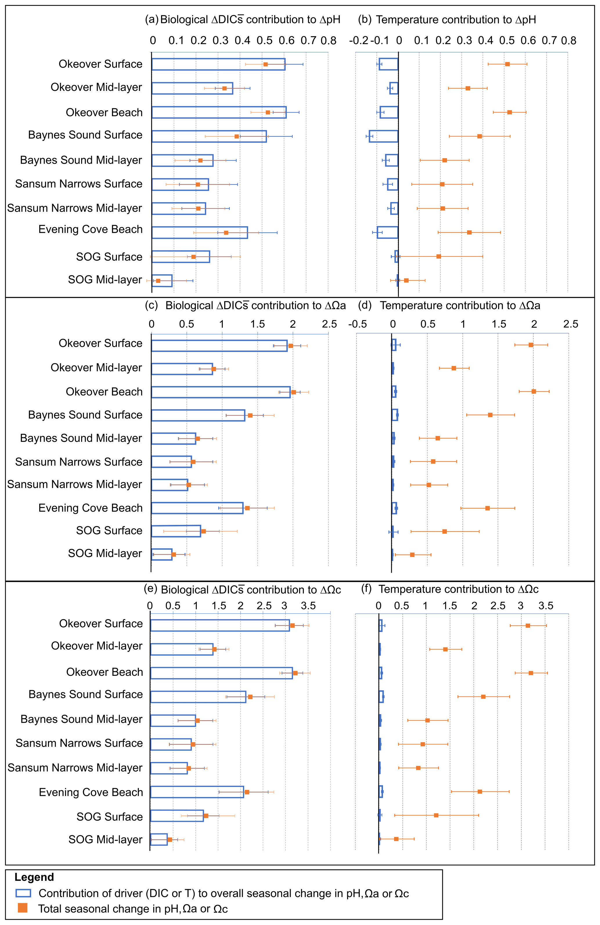
Figure 5 For each location, contribution of seasonal (winter to summer) biologically driven change in salinity-normalized dissolved inorganic carbon (DIC${}_{\stackrel{\mathrm{‾}}{s}}$) (left column) and seasonal temperature change (right column) to seasonal change in pH (a, b), Ω_a (c, d), and Ω_c (e, f) (blue bars), respectively. Total seasonal change in pH, Ω_a, and Ω_c resulting from all contributing drivers is shown in orange on each panel for comparison. Error bars are estimated from combining uncertainty from measurement, seasonal averaging, and partial derivative calculations (Sect. A3).

Table 1 Seasonal differences (summer minus winter) in mean salinity-normalized dissolved inorganic carbon salinity-normalized total alkalinity, salinity, temperature pH, Ω_a, and Ω_c at each location (Sect. 2.3). $\mathrm{\Delta }{\mathrm{DIC}}_{\stackrel{\mathrm{‾}}{\mathrm{s}}}$ and $\mathrm{\Delta }{\mathrm{TA}}_{\stackrel{\mathrm{‾}}{\mathrm{s}}}$ are the difference between the salinity-normalized mean summer minus mean winter DIC and TA (Sect. 2.2). ΔS and ΔT are the difference between mean winter and summer salinity and temperature. Uncertainties are shown in parentheses. Values that are greater than uncertainty are highlighted in bold font.

3.2.1 Seasonal pH change

From winter to summer, a seasonal increase in pH is found across all sites (Fig. 5a, Table 1). The magnitude of the seasonal increase in pH ranges from ∼ 0.04 to 0.53 and varies by location and depth. Typically, the greatest seasonal changes occur in the surface and at beach sites, especially in the Okeover sub-region, where the largest seasonal increases in pH occur (beach and surface layer; Table 1). Large seasonal pH differences are even seen in the mid-layer in Okeover Inlet, where seasonal pH change is the same (within uncertainty of each other) as Evening Cove beach and in the surface of Baynes Sound. Seasonal pH change is lower in the surface at Sansum Narrows, which is the same as mid-layer change in Sansum Narrows and Baynes sound and the surface of the SOG (∼ 0.2). Mid-layer seasonal pH changes are lower than at the surface at all sites and are especially low in the SOG (0.04).

The driver contributing the most to seasonal change in pH (ΔpH) is biologically driven change in DIC ($\mathrm{\Delta }{\mathrm{DIC}}_{\stackrel{\mathrm{‾}}{\mathrm{s}}}$), which contributes significantly more to ΔpH than any other driver (Fig. 5a, Table A9). At all locations, $\mathrm{\Delta }{\mathrm{DIC}}_{\stackrel{\mathrm{‾}}{\mathrm{s}}}$-driven pH increases dwarf contributions from other drivers. The largest ΔpH typically corresponds with the largest $\mathrm{\Delta }{\mathrm{DIC}}_{\stackrel{\mathrm{‾}}{\mathrm{s}}}$ (Table 1). Sensitivities of ΔpH to $\mathrm{\Delta }{\mathrm{DIC}}_{\stackrel{\mathrm{‾}}{\mathrm{s}}}$ are similar across all sites (Table A4) and therefore do not appear to influence the regional differences observed in ΔpH (Fig. 5a, b).

The positive temperature change from winter to summer has little influence on seasonal ΔpH. It drives pH in the opposite direction to $\mathrm{\Delta }{\mathrm{DIC}}_{\stackrel{\mathrm{‾}}{\mathrm{s}}}$ (Fig. 5b), decreasing pH from winter to summer. The temperature-driven ΔpH is an order of magnitude less than the biologically driven change (i.e., from $\mathrm{\Delta }{\mathrm{DIC}}_{\stackrel{\mathrm{‾}}{\mathrm{s}}}$) (Fig. 5a, b). ΔT accounts for a larger proportion of surface ΔpH in Baynes Sound and Evening Cove beach than at other locations, as the seasonal difference in temperature at these locations is larger. However, $\mathrm{\Delta }{\mathrm{DIC}}_{\stackrel{\mathrm{‾}}{\mathrm{s}}}$ still drives most ΔpH at these locations. Mid-layer ΔpH in Okeover Inlet appears large, even relative to the ΔpH in the surface at Baynes Sound and Evening Cove, despite having smaller $\mathrm{\Delta }{\mathrm{DIC}}_{\stackrel{\mathrm{‾}}{\mathrm{s}}}$ (Table 1), although uncertainty envelopes overlap. Larger seasonal ΔT at Baynes Sound and at Evening Cove could be driving pH in the opposite direction to $\mathrm{\Delta }{\mathrm{DIC}}_{\stackrel{\mathrm{‾}}{\mathrm{s}}}$, reducing the ΔpH at these locations.

3.2.2 Seasonal change in CaCO₃ saturation states

Saturation states Ω_a and Ω_c also increase from winter to summer, and although the magnitudes of change are different, both Ω_a and Ω_c follow similar patterns of seasonal change (Fig. 5, Table 1). Seasonal changes in Ω (ΔΩ) also follow a similar pattern to pH. Sites with large ΔpH also experience large seasonal ΔΩ. The surface ΔΩ at nearshore locations is large and >1, bringing the almost completely undersaturated Ω_a conditions in winter into supersaturation in summer. The largest ΔΩ_a and ΔΩ_c are found at Okeover beach and in the Okeover Inlet surface layer (ΔΩ_a ∼ 2 and ΔΩ_c ∼ 3).

Typically, mid-layer seasonal Ω_a and Ω_c difference is less than in the surface, except for Sansum Narrows where it is similar, and both the surface and mid-layer ΔΩ in Sansum Narrows are lower than at other nearshore sites. However, in our data, the smallest ΔΩ is seen in the mid-layer of the SOG.

The driver contributing the most to ΔΩ is $\mathrm{\Delta }{\mathrm{DIC}}_{\stackrel{\mathrm{‾}}{\mathrm{s}}}$, which contributes an order of magnitude more than any other driver (Fig. 5c, e, Table A9). At most locations, $\mathrm{\Delta }{\mathrm{DIC}}_{\stackrel{\mathrm{‾}}{\mathrm{s}}}$ change accounts for all of the seasonal variability in Ω_a and Ω_c. Temperature has less effect on ΔΩ than it does on ΔpH and, unlike pH, drives Ω in the same direction as $\mathrm{\Delta }{\mathrm{DIC}}_{\stackrel{\mathrm{‾}}{\mathrm{s}}}$, i.e., causing a further increase in Ω in summer. Like pH, the largest ΔΩ typically corresponds with the largest $\mathrm{\Delta }{\mathrm{DIC}}_{\stackrel{\mathrm{‾}}{\mathrm{s}}}$ (Table 1), and sensitivities of Ω to $\mathrm{\Delta }{\mathrm{DIC}}_{\stackrel{\mathrm{‾}}{\mathrm{s}}}$ are similar across all sites (Table A4).

3.3 Daily variability

3.3.1 Temperature and salinity

There is little variability (no more than 1.1 °C) in winter T on the days that we investigated (Sect. 2.4) (Fig. 4b, Table 2). In summer, Baynes Sound experiences little T variability (<1 °C) in summer, but T varies by ∼ 2 to 3 °C at the other nearshore locations. Sansum Narrows has the greatest variability in diel summer T (4.4 °C). There is typically low diel variability in S in both seasons (Fig. 4c, Table 2). However, Baynes Sound experiences a large range in diel S on the winter day, spanning from 22 to 28. This larger diel variability was driven by heavy rainfall during the week preceding our sampling (17 November 2017), which also reduced the median surface S to 22.5. Some summer diel variability is also detected in Sansum Narrows as S decreases from 28 to 26 over the day, as new water is brought in with tides.

3.3.2 DIC and TA

Winter diel variability in both DIC and TA is low at Sansum Narrows and Evening Cove beach where the salinity range is low, but variability is high in Baynes Sound, following the large variability in salinity. Variability in summer DIC is greater than in winter at most locations, as biological fluxes during this productive season decrease DIC into the afternoon (Fig. 4d). In contrast, we found almost no summer diel variability in DIC in Baynes Sound in our observations. Variability in summer TA (Fig. 4f) is negligible and either within or close to uncertainty (Table 2).

We investigate the summer day in Okeover during the unusual coccolithophore bloom (August 2016). Total alkalinity has been drawn down as the coccolithophores take up and use dissolved CO${}_{\mathrm{3}}^{\mathrm{2}-}$ to build their shells. The mean TA drawdown is approximately 140 µmol kg⁻¹ compared to “typical summer” conditions (at the same salinity), resulting in a reduction of pH by −0.3, Ω_a by −1.4, and Ω_c by −2.2. There appears to be no diel TA change on the day that we sampled, when the bloom was already well developed (Table 2). Diel DIC change during the coccolithophore bloom is lower than at other locations, but overall DIC is lower, and median DIC (∼ 1550 µmol kg⁻¹) is similar to a “typical summer”, indicating that DIC drawdown has already occurred on a longer temporal scale.

3.3.3 Dissolved oxygen

Winter DO was undersaturated on our sampled days in Baynes Sound and Sansum Narrows, with little variability over the day at both locations (Fig. 4a). The beach location in Evening Cove, however, has higher DO on the sampled day, with some oversaturation occurring in the afternoon. Dissolved oxygen tends to increase throughout the day at the beach site in winter, and all of our nearshore locations in summer, when there is widespread DO supersaturation. Sansum Narrows has the lowest summer saturation state of the four locations, with a smaller increase over the day, resulting in lower variability.

3.3.4 pH

In our observations, the maximum winter diel pH variability is lower than in summer at all locations. Winter diel pH variability is higher (∼ 0.2 to 0.3) in Baynes Sound and Evening Cove beach than in Sansum Narrows. At the beach, winter pH increases throughout the morning into the afternoon, whereas winter pH in Baynes Sound does not increase over the day but fluctuates with salinity (Fig. 4h). In summer, pH is higher than winter and pH variability is higher at Evening Cove and Sansum Narrows, but it is lower in Baynes Sound.

3.3.5 Saturations states Ω_a and Ω_c

In our observations, winter diel Ω_a variability is low in Baynes Sound and Sansum Narrows, but up to ∼ 0.6 at Evening Cove beach, as Ω_a increases over the course of the day (Fig. 4i). Winter variability in Ω_c is similar to Ω_a, with low variability in Baynes Sound and Sansum Narrows, and greater variability at the beach. In our observations at all locations, there is greater diel variability in Ω_a and Ω_c in summer as saturation states increase throughout the day.

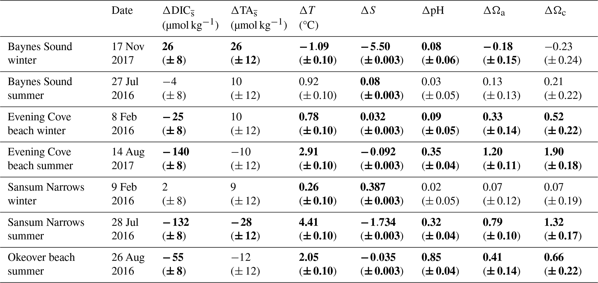
Table 2 Maximum observed change in salinity-normalized dissolved inorganic carbon, salinity normalized total alkalinity, salinity, temperature, pH, and Ω in the surface layer (0 to 5 m) over the course of a single day at each location (Sect. 2.4). $\mathrm{\Delta }{\mathrm{DIC}}_{\stackrel{\mathrm{‾}}{\mathrm{s}}}$ and $\mathrm{\Delta }{\mathrm{TA}}_{\stackrel{\mathrm{‾}}{\mathrm{s}}}$ are determined from the difference between the earliest (morning), and latest (mid-afternoon) normalized DIC and TA recorded in the day. ΔS and ΔT are calculated as the difference between the earliest (morning), and latest (mid-afternoon) S and T. Uncertainties are shown in parentheses. Values that are greater than uncertainty are highlighted in bold font.

3.4 Drivers of diel change in carbonate chemistry

3.4.1 Winter

Winter diel ΔpH and ΔΩ are small, mostly driven by small contributions from biologically driven change in DIC ($\mathrm{\Delta }{\mathrm{DIC}}_{\stackrel{\mathrm{‾}}{\mathrm{s}}}$) (Table A10). Primary production is low in winter and therefore smaller $\mathrm{\Delta }{\mathrm{DIC}}_{\stackrel{\mathrm{‾}}{\mathrm{s}}}$ drives small diel ΔpH or ΔΩ at all three sites (Table 2). Biological TA contribution ($\mathrm{\Delta }{\mathrm{TA}}_{\stackrel{\mathrm{‾}}{\mathrm{s}}}$) to diel ΔpH and ΔΩ in winter is most often negligible (i.e., within uncertainty). Freshwater and diel ΔT are both negligible drivers of diel ΔpH and ΔΩ at all sites in winter. There are no detectable diel ΔpH and ΔΩ in Sansum Narrows in winter, but some small diel changes (beyond, but close to uncertainty) are detected in Baynes Sound and at Evening Cove beach. Small increases in pH and Ω are detectable at Evening Cove beach in winter, driven by biological drawdown of DIC, as the calm, clear day progressed (Table A10).

In Baynes Sound, a small pH increase of 0.08 (± 0.06) is detected over the winter day. The estimated ΔpH from $\mathrm{\Delta }{\mathrm{DIC}}_{\stackrel{\mathrm{‾}}{\mathrm{s}}}$ on this day is negative (−0.09 ± 0.03), suggesting that a small amount of remineralization may have occurred. At most locations $\mathrm{\Delta }{\mathrm{TA}}_{\stackrel{\mathrm{‾}}{\mathrm{s}}}$ and freshwater are negligible drivers of carbonate parameters (Table A10). However, on the winter day in Baynes Sound, a diel ${\mathrm{TA}}_{\stackrel{\mathrm{‾}}{\mathrm{s}}}$ increase (∼ 26 µmol kg⁻¹) increases pH by 0.09 (± 0.05), countering the decrease driven by $\mathrm{\Delta }{\mathrm{DIC}}_{\stackrel{\mathrm{‾}}{\mathrm{s}}}$. This TA increase also drives an increase in saturation states of 0.24 (± 0.12) Ω_a and 0.38 (± 0.19) Ω_c. A small freshwater contribution is also detected at Baynes Sound, where a decrease in salinity of ∼ 5 over the day contributes to a 0.07 (± 0.014) increase in pH and 0.2 (± 0.02) decrease in both Ω_a and Ω_c. However, the diel changes in Ω_a and Ω_c in winter at Baynes Sound are essentially negligible (i.e., less than or close to uncertainty) (Table 2).

3.4.2 Summer

Like seasonal change, the main contributing driver of diel ΔpH and ΔΩ is a biologically driven change in DIC ($\mathrm{\Delta }{\mathrm{DIC}}_{\stackrel{\mathrm{‾}}{\mathrm{s}}}$) (Table A10). Typically, large diel changes in pH, Ω_a, and Ω_c occur over the day in summer driven primarily by biological DIC drawdown, although there is no detectable ΔpH or ΔΩ in Baynes Sound in summer (Table 2). Temperature and freshwater have negligible driving effects, and biological ${\mathrm{TA}}_{\stackrel{\mathrm{‾}}{\mathrm{s}}}$ contributions are only detected at Sansum Narrows. The largest pH increase over the day in summer is observed at Evening Cove beach (0.35 ± 0.04), followed by Sansum Narrows (0.32 ± 0.04) and Okeover Inlet (0.85 ± 0.04) (Table 2). Changes in pH driven by $\mathrm{\Delta }{\mathrm{DIC}}_{\stackrel{\mathrm{‾}}{\mathrm{s}}}$ are ∼ 0.4 (± 0.016), ∼ 0.5 (± 0.011), and ∼ 0.2 (± 0.018) at Evening Cove, Sansum Narrows, and Okeover, respectively (Table A10). The largest diel Ω_a increase is also observed at Evening Cove beach, followed by Sansum Narrows and Okeover Inlet, where $\mathrm{\Delta }{\mathrm{DIC}}_{\stackrel{\mathrm{‾}}{\mathrm{s}}}$ contributes to an increase in Ω_a of ∼ 1.3 (± 0.011), ∼ 1 (± 0.05), and ∼ 0.5 (± 0.07), respectively.

Summer temperature increase over the day is the second largest driver of pH, driving a diel decrease in pH at all sites (Table A10). However, this temperature-driven pH decrease is dwarfed by biological DIC and is less than 0.1 at all sites. Temperature also has a negligible driving effect on saturation states, increasing saturation states no more than 0.04.

Our estimated biological ${\mathrm{TA}}_{\stackrel{\mathrm{‾}}{\mathrm{s}}}$ contributions to diel summer pH and Ω change are mostly within uncertainty (Table A10). However, at Sansum Narrows, a small ${\mathrm{TA}}_{\stackrel{\mathrm{‾}}{\mathrm{s}}}$ decrease of 28 µmol kg⁻¹ contributes to a decline in diel pH of −0.1 (± 0.04) and a decrease in Ω_a of 0.2 (± 0.09) and −0.4 (± 0.2) Ω_c, which could indicate uptake of CaCO₃ by calcifiers at this site. There is no detectable ΔTA- or TA-driven ΔpH or ΔΩ during the summer day in Okeover, during the coccolithophore bloom.

4 Discussion

4.1 Variability

At the nearshore locations, variability in pH and Ω is low in winter and high in summer. High summer variability is due to strong variability in primary production on the synoptic scale, as blooms come and go (e.g., Moore-Maley et al., 2016). When we sampled, we typically captured a different phase of a phytoplankton bloom during each campaign. On a diel scale, in summer, primary production increases both pH and Ω during the daylight hours, while respiration during the dark hours decreases pH and Ω. In addition, variable weather conditions on different sampling days also result in variability in primary production. For example, light may either limit (e.g., overcast, windy) or enable phytoplankton (e.g., sunny, calm). Wind mixing, following a period in which nutrients were limiting and carbon was drawn down, may provide nutrients and carbon to the surface, resulting in a brief, rapid reduction in pH (Moore-Maley et al., 2017) before stimulating a new bloom (Allen and Wolfe, 2013; Moore-Maley et al., 2016). As primary production is the major driver of higher pH and Ω, low variability in winter is a result of lower primary production, due to phytoplankton growth being light-limited (Harrison et al., 1983; Allen and Wolfe, 2013).

4.2 Drivers of pH and Ω variability

4.2.1 ${\mathrm{DIC}}_{\stackrel{\mathrm{‾}}{\mathrm{s}}}$ and ${\mathrm{TA}}_{\stackrel{\mathrm{‾}}{\mathrm{s}}}$

The dominant driver of seasonal and diel ΔpH and ΔΩ in the Salish Sea is biologically driven DIC change ($\mathrm{\Delta }{\mathrm{DIC}}_{\stackrel{\mathrm{‾}}{\mathrm{s}}}$), which contributes an order of magnitude more to seasonal and diel ΔpH and ΔΩ than any other driver. At our locations, $\mathrm{\Delta }{\mathrm{DIC}}_{\stackrel{\mathrm{‾}}{\mathrm{s}}}$ is caused by the consumption of carbon by primary production in spring–summer, which greatly outweighs any remineralization signal. Drawdown of DIC occurs during periods of high oxygen saturation, indicating that DIC is drawn down by primary production (Figs. 2a, 3a, 4a). While low light limits primary production in winter, strong spring–summer blooms are triggered when this light limitation is lifted (Harrison et al., 1983; Allen and Wolfe, 2013), resulting in the large seasonal differences in DIC, pH, and Ω observed at the surface.

Seasonal variability in pH and Ω is higher in the surface layer (0 to 5 m) than the mid-layer (5 to 20 m) at all locations because of greater spring–summer production and the resulting, large $\mathrm{\Delta }{\mathrm{DIC}}_{\stackrel{\mathrm{‾}}{\mathrm{s}}}$ in the surface. Our study locations are often highly stratified, with a fresher, less dense, surface layer which extends to ∼ 5 m depth. Stratification limits mixing and holds phytoplankton in the photic zone of the surface layer, which prevents light limitation and results in large drawdown of DIC at the surface. The effects of this primary production are observed in the summer diel results, where DIC drawdown throughout the day results in a diel pH and Ω increase. Although seasonal and diel changes in the more light-limited mid-layer are less prominent than in the surface, variability in pH and Ω are still observed. Spring–summer pH and Ω in the mid-layer are not as elevated as in the surface but are higher in summer, as mid-layer waters mix with the DIC depleted and high pH and Ω waters of the surface layer.

Biological modulation of DIC is the major driver of seasonal and diel ΔpH and ΔΩ in the Salish Sea, as the region is highly sensitive to changes in DIC (Simpson et al., 2022; Jarníková et al., 2022b). The Salish Sea region is sensitive as it is carbon rich (Ianson et al., 2016), due to long sub-surface residence times (Masson, 2002; Pawlowicz et al., 2007) that allow remineralized DIC to accumulate. TA is also relatively high, and DIC : TA ratios are close to 1, which places the Salish Sea in highly sensitive carbonate space, where small changes in DIC result in large changes in pH and Ω (e.g., Egleston et al., 2010; Hu and Cai, 2013; Simpson et al., 2022; Moore-Maley et al., 2018). Processes that modulate the high DIC content in this sensitive system are therefore the main contributing drivers of pH and Ω change in the Salish Sea. Partial derivatives of pH and Ω (with respect to DIC) across locations were similar, indicating little variability in this high sensitivity throughout the Salish Sea (Table A4). The largest seasonal and diel ΔpH and ΔΩ were found where the greatest $\mathrm{\Delta }{\mathrm{DIC}}_{\stackrel{\mathrm{‾}}{\mathrm{s}}}$ occurred. The magnitude of $\mathrm{\Delta }{\mathrm{DIC}}_{\stackrel{\mathrm{‾}}{\mathrm{s}}}$ (i.e., how productive a system is), rather than sensitivity, is therefore responsible for the difference in pH and Ω variability observed at different nearshore locations on both diel and seasonal scales.

As the magnitude of DIC drawdown by primary production in spring–summer is key to driving high pH and Ω conditions which are favourable to calcifiers, any future changes to phytoplankton abundance or assemblage would likely have strong implications for OA in this region. Increased temperatures since 1999 have been linked to increased stratification and a reduction in nutrient renewal in the surface ocean on a global scale, which in turn has reduced global primary production (Behrenfeld et al., 2006). Regionally, the ∼ 4 °C temperature anomaly known as to the “Pacific Blob” event reduced primary production in the coastal waters outside of the Salish Sea (Peña et al., 2018). Higher temperatures projected to occur with climate change could therefore limit the seasonal modulation of low to high pH and Ω in winter to summer by primary production in the already stratified Salish Sea, prolonging low pH and Ω undersaturation conditions.

Biologically driven changes in TA from biomineralization of CaCO₃ or dissolution of shells could also drive large changes in pH and Ω due to the high sensitivity of the system, if they were greater. These fluxes ($\mathrm{\Delta }{\mathrm{TA}}_{\stackrel{\mathrm{‾}}{\mathrm{s}}}$) in our study, if present, are too small to detect and likely do not drive changes in pH or Ω in our system. In the future, biologically driven TA changes could become a more important driver of seasonal change in summer, as increased temperatures increase the likelihood of calcifying coccolithophore blooms (Rivero-Calle et al., 2015; Harada et al., 2012). The coccolithophore bloom captured in 2016 was the only recorded bloom of this type, which occurred during particularly warm conditions. Although it had no effect on a diel scale, the coccolithophore bloom did have an impact on pH and Ω (reduction in pH by −1.4, and Ω_a by −2.2) compared to a “typical” summer.

4.2.2 Temperature

In our region, temperature drives relatively small changes in carbonate parameters relative to the large variability driven by DIC. Warming decreases pH and therefore counters the effect of DIC drawdown on pH on both seasonal and diel timescales, but it has little direct influence on Ω. Although it is the second largest driver, the contribution of seasonal temperature change is small at all locations, and pH changes resulting from this seasonal temperature difference are low (mostly <0.1). Where diel temperature changes in summer are relatively high (i.e., Sansum Narrows), the temperature contribution to pH decrease still remains <0.1. Temperature, therefore, is not a notable driver of diel or seasonal changes in pH and Ω in this region as it is dwarfed by the biological fluxes of DIC.

4.2.3 Freshwater

Freshwater influence is a negligible driver of pH and Ω change at nearshore locations in the Salish Sea, despite strong salinity gradients and the strong salinity control of both DIC and TA in the region (Ianson et al., 2016; Simpson et al., 2022). The SOG is characterized by estuarine circulation (LeBlond, 1983), with a relatively fresh surface layer that receives large riverine inputs primarily from the Fraser River (Moore-Maley et al., 2018) and a multitude of other, mainly pluvial rivers (Morrison et al., 2011). The large spring–summer input of freshwater received from the glacial freshet appears balanced by the large pluvial inputs in fall and winter when this region receives heavy rainfall. As a result, there is little change in salinity between seasons (typically a decrease between 0.4 and 1.7 from winter to summer), which is too minor to drive seasonal change in pH or Ω.

Where larger salinity changes occur (e.g., during significant rain events on a diel scale, such as in Baynes Sound in winter), ΔpH and ΔΩ are driven by the ΔS being large enough to shift carbonate system constants. DIC and TA changes driven by ΔS have negligible driving effects on pH and Ω as both DIC and TA shift together. In the Salish Sea, TA and DIC mixing lines run almost parallel to one another (Simpson et al., 2022), so shifting DIC and TA in response to ΔS keeps the DIC : TA ratio similar, and thus pH and Ω remain similar. In other words, ΔDIC and ΔTA resulting from ΔS shift pH and Ω in almost equal and opposite directions in this region, resulting in only minor ΔpH and ΔΩ (Tables A9, A10). These minor changes are negligible in relation to those driven by biological ΔDIC.

Despite being a minor driver of seasonal and diel change in carbonate parameters in the Salish Sea, salinity determines the sensitivity of the system to changing DIC. Freshwater input and salinity change are important as they determine the magnitude of the effect of the major driver, $\mathrm{\Delta }{\mathrm{DIC}}_{\stackrel{\mathrm{‾}}{\mathrm{s}}}$, on ΔpH and ΔΩ. The Salish Sea is highly sensitive throughout, and thus ΔS does not change the sensitivity significantly (Simpson et al., 2022; Jarníková et al., 2022b). In other estuarine environments, where DIC and TA mixing lines do not run parallel (e.g., Hu and Cai, 2013), freshwater-induced salinity change could be a more significant driver. In these systems, carbonate system sensitivities to ΔDIC (e.g, βDIC) can significantly change as salinity decreases, resulting in larger ΔpH and ΔΩ for the same change in DIC (Hu and Cai, 2013).

4.3 Variability and drivers at each location

4.3.1 Okeover Inlet

Okeover Inlet stands out from other nearshore locations as it has higher surface pH and Ω than other nearshore sites. These conditions are driven by higher primary production in summer, which is indicated by Okeover having some of the highest oxygen saturations of all nearshore locations. Okeover also has the greatest seasonal ΔpH and ΔΩ, driven by the largest seasonal $\mathrm{\Delta }{\mathrm{DIC}}_{\stackrel{\mathrm{‾}}{\mathrm{s}}}$ from primary production. Higher primary production is likely a result of Okeover Inlet containing high subsurface nutrients (Fig. A1) as well as from experiencing frequent calm stratified conditions which prevent light limitation and periodic wind mixing of nutrient-rich water into the surface layer. Okeover Inlet is connected to the rest of the Salish Sea through the shallow and narrow Malaspina Inlet, which limits exchange of water between Okeover Inlet and the NSOG. This isolation of the Inlet results in nutrient trapping (e.g., Ianson et al., 2003), as long residence times allow for continued primary production, drawdown of DIC, and elevated pH and Ω in the surface in summer. High primary production at the surface contributes to concentrated nutrients in deeper waters from high organic rain, compounded by limited mixing with outside waters and a relatively small volume of water. This subsurface nutrient trapping can further enhance low pH and Ω at the surface, when these subsurface waters with high nutrient concentrations are mixed into the surface during wind events and stimulate primary production. In our observations, Okeover is also cooler than other locations in summer (with the exception of the coccolithophore bloom year), which may reduce the risk of temperature-induced mortality of shellfish in this region as temperatures increase with climate change.

During the unusual coccolithophore bloom in Okeover Inlet in 2016 (NASA, 2016), TA was drawn down (in comparison to a “typical” summer) because of plate-building uptake of CO${}_{\mathrm{3}}^{\mathrm{2}-}$ by coccolithophores. However, there was no detectable biological drawdown of TA on a diel scale during this bloom, likely because bio-formation of CaCO₃ plates had already occurred. Diel ${\mathrm{DIC}}_{\stackrel{\mathrm{‾}}{\mathrm{s}}}$ contribution to pH and Ω change during the coccolithophore bloom was lower than ${\mathrm{DIC}}_{\stackrel{\mathrm{‾}}{\mathrm{s}}}$ contribution from “typical” conditions at other nearshore sites. It is possible that the increase in turbidity from the coccolithophores (Secchi depth ∼ 0.5 m in comparison to ∼ 5.5 m during “typical” conditions) limited light required for primary production, and the bloom was already well developed. However, significantly more data from both typical and atypical blooms would be required to examine the differences in $\mathrm{\Delta }{\mathrm{DIC}}_{\stackrel{\mathrm{‾}}{\mathrm{s}}}$ with certainty.

4.3.2 Beach grow locations

Conditions at beach grow locations do not stand out from the surface layer of other nearshore locations, suggesting no clear advantage of a beach lease compared to a surface tray hang to shellfish growers. At Okeover and Evening Cove beaches, we did not observe any clear differences in terms of more elevated pH and Ω, greater variability, or greater seasonal change in carbonate chemistry, when compared with other nearshore locations. Primary production and associated DIC drawdown at the beach sites is similar to that in the surface layer in other locations where shellfish are grown, indicated by similar $\mathrm{\Delta }{\mathrm{DIC}}_{\stackrel{\mathrm{‾}}{\mathrm{s}}}$ and oxygen saturation. There were also no clear indications of pH elevation related to TA increase at the shell midden beach location in Okeover over other beaches or other nearshore sites. Diel temperature increase at the beach locations was also similar to the surface layer at other sites. This similarity between shallow beach sites and the surface layer (0 to 5 m) of other locations is likely due to a moderate tidal range (3 to 4 m) and a similar level of primary production throughout the nearshore. However, the highest median temperature was found at Evening Cove beach, ∼ 4 °C higher than most locations. Given the association between shellfish mortality and high temperatures (Wendling et al., 2014; King et al., 2019), as temperatures increase, shellfish farmers considering future grow locations may wish to choose a tray hang location rather than a beach grow site, to provide the option to drop trays deeper in the water column where temperatures are cooler to reduce heat stress.

4.3.3 Baynes Sound

Baynes Sound has the highest density of shellfish operations in the Salish Sea (Holden et al., 2019), high summer pH and Ω, and large seasonal changes in surface pH and Ω driven by drawdown of DIC by primary production. The seasonal increase in pH and Ω driven by primary production is relatively high in Baynes Sound as it is continuously supplied with nutrients from the north (Olson et al., 2020) and from a deep SOG tidal injection from the south (Guyondet et al., 2022). Like Okeover Inlet, high nutrients provide conditions that enable primary production. However, in contrast to Okeover Inlet, Baynes Sound is not a nutrient trap, as it is well connected to the SOG and to a continual re-supply of nutrients, which prevents nutrient limitation in the surface layer throughout spring–summer.

Despite high primary production driving strong seasonal changes, Baynes Sound is the only location to have minimal to no diel summer pH and Ω increase and little to no biologically driven change in DIC over the day. The absence of diel pH or Ω increase in Baynes Sound might be explained by the number of commercially grown shellfish feeding on phytoplankton, which could be reducing the standing stock of primary producers enough to reduce the local biological drawdown of DIC. A recent study has indicated that shellfish aquaculture in Baynes Sound is currently operating within the ecological carrying capacity and that cultured bivalves consume phytoplankton at a rate that reduces net production by up to ∼ 30 % in Deep Bay (Guyondet et al., 2022), which would decrease, but not remove, the diel ΔDIC. Our Baynes Sound site is relatively shallow (<20 m), and another explanation for the absence of diel changes could be that a respiration signal from the benthic zone is countering the drawdown of DIC by primary production. However, neither a reduction in primary production nor a significant respiration signal appears likely, as oxygen saturation percentages are high even at the bottom of Baynes Sound (Fig. A1). As pH, Ω, and oxygen saturation remain high, another explanation for why a diel change is not observed in summer is that Baynes Sound is rapidly flushed with a residence time on the order of weeks (Guyondet et al., 2022). The rapid flushing of water masses could maintain stable DIC, pH, and Ω conditions at the location of sampling, although primary production is still occurring.

4.3.4 Sansum Narrows

Strong tidally mixed areas have low variability and lower seasonal change in pH and Ω. Sansum Narrows is characterized by rapid tidal streams flushing and mixing water through the narrow channels. As a result of this mixing, surface variability is similar to that found in the mid-layer and much lower than the surface variability observed elsewhere. Nutrients are always replete in Sansum Narrows as they are renewed at the surface by mixing (Fig. A1), enabling primary production, which is the main driver of pH and Ω variability and seasonal change. The distinct differences between surface and mid-layer found at other locations are not observed at Sansum Narrows as the effect of DIC drawdown is diluted through a greater depth of the water column by mixing. Lower oxygen saturation at the surface in Sansum Narrows than at other locations (Fig. 2) indicates that phytoplankton are affected by light limitation as they (and the oxygen that they produce) are mixed down away from the photic zone. As a result, pH and Ω do not become as elevated as other locations in summer, and Sansum Narrows has the lowest (but most steady) pH and Ω of the nearshore locations, which can sometimes be lower than the open waters of the SOG.

4.3.5 SOG

The open waters of the SOG appear to be as variable as the nearshore from our data but have lower summer pH and Ω than most nearshore sites and a smaller seasonal surface change in pH and Ω. The open waters of the SOG are not as productive in the surface layer as the nearshore sites, as dense phytoplankton blooms are supported in the nearshore at times when blooms in the open waters are not. Weaker blooms in the open waters are likely more limited by greater mixing than in the nearshore. As a result, the surface SOG experiences a much smaller $\mathrm{\Delta }{\mathrm{DIC}}_{\stackrel{\mathrm{‾}}{\mathrm{s}}}$ and a smaller seasonal change in pH and Ω than in the nearshore.

5 Conclusions and implications

The large seasonal and diel variability observed at the nearshore locations implies that shellfish are already exposed to large ranges and extremes of pH and Ω in the Salish Sea, including low pH and undersaturation of Ω_a, and even some undersaturation of Ω_c, in winter. The largest variability and seasonal change in pH and Ω are found at the surface and at beaches where most commercially grown and wild shellfish are present. Although the open waters of the SOG are, like the nearshore, highly variable, pH and Ω are lower in the open waters than in the nearshore in summer, and seasonal changes in pH and Ω are relatively small. Our results suggest that ship-based data collection in open waters is not adequate for characterizing the variability and the extremes experienced in the nearshore.

DIC drawdown by primary production is the dominant driver of seasonal and diel pH and Ω change at nearshore locations and creates favourable conditions for shellfish in summer. Temperature, although important because of its link to shellfish disease, has a less important role with respect to the carbonate system. Temperature increase drives pH down from winter to summer, but the effect is an order of magnitude smaller than the change in pH driven by DIC uptake by phytoplankton. Temperature is therefore a minor driver of ΔpH and ΔΩ on seasonal and diel scales at the surface and beach locations and has a negligible effect in the mid-layer. Although shellfish themselves do have the ability to alter the carbonate chemistry in their surrounding environment through shell building or dissolution, the resulting biological change in TA and associated change in pH and Ω are too small to detect. Even in dense shellfish aquaculture operations such as Baynes Sound, where aquaculture is significant enough to alter primary production on a local scale (Guyondet et al., 2022), no detectable TA signal was observed. There was also no detectable TA change or increase at the shell midden beach location in Okeover. Our results suggest that freshwater is a negligible driver of seasonal and diel changes in pH and Ω in temperate fjords, as summer glacial and winter pluvial freshwater inputs are similar in magnitude. Salinity variability is a main control of variability in DIC and TA, but seasonal and diel change in salinity is not enough to drive notable changes in pH and Ω (Figs. 2–4). Salinity is, however, still an important control of pH and Ω sensitivities to DIC change (e.g., Hu and Cai, 2013; Simpson et al., 2022).

Winter pH conditions in the Salish Sea are well below the present-day global average of 8.1 (Raven et al., 2005; Jiang et al., 2019) (i.e., 7.6 to 7.8), and Ω_a is persistently undersaturated. Although diel variability in winter may at times bring the beach locations out of Ω_a undersaturation briefly, undersaturation of Ω_a persists in winter at most locations. Aragonite is primarily used by calcifying organisms to build shells at the early life stages (Waldbusser et al., 2015), and so this chronic winter Ω_a undersaturation is of significance to the timing of out-planting oyster seed. To avoid unfavourable Ω_a conditions, seed could be out-planted after the onset of the spring bloom when local surface conditions rapidly become supersaturated (Moore-Maley et al., 2016). Out-planting of vulnerable shellfish seed and juveniles is typically already carried out in summer, avoiding stressful conditions. At present, the summer shellfish growing period experiences high Ω_a, greater than 1.5, which is favourable to shellfish growth (Waldbusser et al., 2015); summer pH values at our nearshore locations are above the present-day global averages.

Although OA may cause stress by increasing energy expenditure in shellfish (e.g., Pousse et al., 2020), OA does not appear to be directly responsible for mortality events in our region. Most shellfish mortality events recorded in the Salish Sea have occurred in summer (Cowan et al., 2020; Morin, 2020; King et al., 2021) when pH and Ω_a are relatively high, and not in winter when chronic undersaturation of Ω_a and some Ω_c undersaturation occurs (Fig. 3b, c). Higher temperatures linked to disease appear to be a more immediate concern to shellfish growers in the Salish Sea (e.g., Morin, 2020). It is possible that wild shellfish have adapted to, or that commercial shellfish species are already tolerant of, this chronic exposure to lower Ω_a conditions in winter (e.g., Waldbusser et al., 2016). Additionally, values of Ω_c (which are mostly supersaturated) rather than Ω_a are likely more relevant to shellfish during winter because juveniles are typically out-planted in summer and have reached maturity and transitioned to calcite structures by winter (e.g., Stenzel, 1964).

Growers may wish to consider placing shellfish, especially juveniles, deeper than the surface layer in summer where temperatures are lower, and oxygen and carbonate chemistry conditions are still favourable for shellfish growth. Temperatures in the mid-layer are cooler, and although pH tends to be slightly lower, the mid-layer mostly remains supersaturated with respect to both Ω_a and Ω_c in summer (Figs. 2, 3). In addition, beaches do not appear to have a clear advantage over tray hang sites in terms of carbonate chemistry. However, beach sites experience the highest temperatures of all locations and may become less favourable locations in the future as temperature rises (e.g., Hesketh and Harley, 2023). Indeed, extreme heat events have already caused mass mortalities of invertebrates in the inter-tidal areas of the Salish Sea (White et al., 2021).

OA is projected to reduce pH and Ω in the coming decades, and the favourable summer conditions currently observed in the Salish Sea may become less favourable, especially as pH and Ω in the Salish Sea are highly sensitive to DIC change (Jarníková et al., 2022b; Simpson et al., 2022). Chronic Ω_a, and even some Ω_c, undersaturation already occurs in winter. Undersaturated Ω_c conditions will likely become more common and widespread in the future (e.g., Hauri et al., 2013), increasing stress for adult shellfish in the winter season. The shift towards more stressful carbonate conditions in winter, combined with higher temperatures in summer, could result in chronic exposure of calcifiers to stressful environmental conditions. Okeover Inlet is highly productive in summer, and as a result shellfish aquaculture tenures in that region are likely less vulnerable to increasing acidification due to elevated pH and Ω and lower sensitivities to changes in the carbonate system in summer. Sansum Narrows is tidally mixed, and as a result pH and Ω are presently lower than at other locations, as primary production is limited as phytoplankton are removed from the surface by mixing. Beach grow locations have similar pH and Ω to other nearshore locations, but aquaculture tenures in these areas are exposed to the highest summer temperatures.

Appendix A

A1 Endmembers

South strait of Georgia endmember

To define our south SOG (SSOG) endmember (the salty endmember for the Sansum Narrows and Evening Cove sites), we used ship-collected data, collected between 2003–2012 from sampling stations in the SSOG and nearby waters (Stations 42, 46, 56, and 59 in Ianson et al., 2016). The Sansum Narrows region is strongly mixed, as is incoming water from the SSOG, east of Satellite Channel from Haro Strait. Well-mixed water from the SOG therefore likely enters Sansum Narrows at the 70 m sill of Satellite Channel. We use an average of data from 75–250 m to define the salty endmember in Table A2 (e.g., Simpson et al., 2022). We also considered endmembers with shallower mixing depths closer to the sill depth of 75 m; these fell on the same salinity–DIC and salinity–TA relationship lines as our selected endmember, but they were too fresh to capture all the salinity range in our observational data.

Fraser River endmember

The Fraser River endmember was determined from a single sample taken in New Westminster, BC, in March 2017.

Cowichan River endmember

The Cowichan River is a large river with high discharge and is likely the most influential freshwater source throughout the Sansum Narrows area and at Evening Cove beach. We calculated DIC–S and TA–S relationships with several freshwater sources and the same SSOG salty endmember and assessed the fit of observational data to these relationships. We found that DIC–S and TA–S mixing lines calculated from water properties of the Cowichan River and the SSOG salty endmember fit best with observations from Sansum Narrows and Evening Cove. The mean DIC and TA collected from the same upstream location of the Cowichan River were used for this fresh endmember.

A2 Partial derivative calculations

Partial derivatives were calculated at site-specific mean annual salinity (Sect. 2.4, Table A3). Due to the large range in S present at each nearshore location and the strong control S has on the carbonate system, we use an annual mean S (${\stackrel{\mathrm{‾}}{S}}_{\mathrm{annual}}$) that is location and depth specific, for our partial derivative calculations. We normalize all observational DIC and TA to the appropriate ${\stackrel{\mathrm{‾}}{S}}_{\mathrm{annual}}$, following Friis et al. (2003; Sect. 2.3), to present typical conditions. Finally, for each location and depth, we solve the carbonate system, using the location- and depth-specific mean annual ${\mathrm{DIC}}_{\stackrel{\mathrm{‾}}{\mathrm{s}}}$ and ${\mathrm{TA}}_{\stackrel{\mathrm{‾}}{\mathrm{s}}}$, T, S, and nutrients (Table A3), to yield the partial derivatives (Table A4).

A3 Uncertainty in Taylor expansion results

While most previous ocean studies that use Taylor expansions do not consider uncertainty, our data cover exceptionally wide ranges in salinity and carbonate chemistry parameters (e.g., Fig. 2). Thus, we estimate the uncertainty in the contributions of each driving component, i.e., each term in a given expansion (Eqs. 1–6). For example, consider the contribution of T to seasonal variability in pH: we estimate the uncertainty of the partial derivative ($\partial \mathrm{pH}/\partial T$) and the seasonal range (ΔT) (term 3 on the right-hand side of Eq. 1). The uncertainty estimation for each driving component is discussed in detail the following subsection.

Partial derivative uncertainty

The partial derivatives used in the Taylor expansion are determined at annual mean conditions for each location. More specifically, they are calculated at a mean salinity and temperature with ${\mathrm{DIC}}_{\stackrel{\mathrm{‾}}{\mathrm{s}}}$ and ${\mathrm{TA}}_{\stackrel{\mathrm{‾}}{\mathrm{s}}}$ (Sect. A2). We estimate the uncertainty in our derivatives from the uncertainty envelope of the seasonal change of each driving component. For example, we add or subtract the uncertainty in the seasonal change in T from the annual mean T and recalculate the derivatives (e.g., $\partial \mathrm{pH}/\partial T$).

Seasonal and diel change uncertainty

To calculate the uncertainty in the seasonal differences of driving components (e.g., ΔT), we took the geometric mean of uncertainty in mean summer conditions (standard error), mean winter conditions (standard error), and measurement uncertainty (pooled standard deviation of replicates; see Simpson et al., 2022) (Tables A5, A6).

Freshwater term uncertainty

Uncertainty in the freshwater term (Eqs. 4–6) was calculated from the uncertainty in ΔpH, ΔΩ_a, or ΔΩ_c driven by seasonal or diel ΔS. The ranges in ΔDIC and ΔTA corresponding to the uncertainty envelope of ΔS (as above) were calculated, and ΔpH, ΔΩ_a, and ΔΩ_c were recalculated with these DIC and TA ranges. For example, the seasonal ΔS at Okeover beach was −1.2 ± 0.7. We calculated the change in DIC and TA resulting from an increase and a decrease in S of 0.7. These DIC and TA pairs were then used to resolve the carbonate system, keeping all other parameters (except for S) the same. The resulting range in pH, Ω_a, and Ω_c is the freshwater uncertainty envelope for these parameters.

Table A1 Name and location of fresh and salty endmembers used for establishing the DIC–S and TA–S relationships used when normalizing DIC and TA to annual S at each location (Fig. 1). See Simpson et al. (2022), their Sect. A5, and text below for details on how the Cowichan River, Fraser River, and SSOG endmembers were determined.

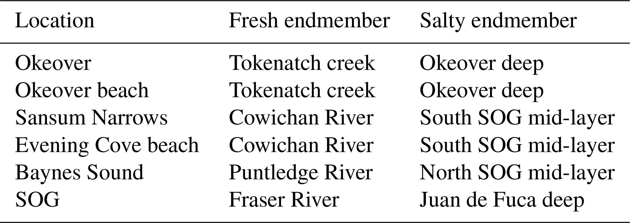
Table A2 Fresh and salty endmember chemical properties: salinity (S), dissolved inorganic carbon (DIC), and total alkalinity (TA).

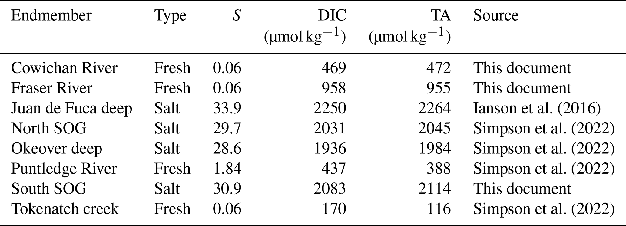
Table A3 Values used to solve the carbonate system for partial derivative calculations. Where ${\stackrel{\mathrm{‾}}{S}}_{\mathrm{annual}}$ is the annual mean salinity at the location and depth layer of interest, $\stackrel{\mathrm{‾}}{{\mathrm{DIC}}_{\mathrm{s}}}$ and $\stackrel{\mathrm{‾}}{{\mathrm{TA}}_{\mathrm{s}}}$ are the mean normalized DIC and TA normalized to the location- and depth-specific ${\stackrel{\mathrm{‾}}{S}}_{\mathrm{annual}}$ and where $\stackrel{\mathrm{‾}}{T}$, $\stackrel{\mathrm{‾}}{\mathrm{Si}}$, and $\stackrel{\mathrm{‾}}{{\mathrm{PO}}_{\mathrm{4}}}$ are annual mean values of temperature, silicic acid, and phosphate, and $\stackrel{\mathrm{‾}}{P}$ is mean pressure for the depth layer.

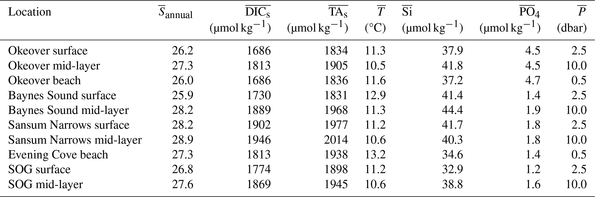
Table A4 Partial derivatives by location and depth (annual mean). OIS – Okeover Inlet surface, OIML – Okeover Inlet mid-layer, OIB – Okeover Inlet beach, BSS – Baynes Sound surface, BSML – Baynes Sound mid-layer, SNS – Sansum Narrows surface, SNML – Sansum Narrows mid-layer, ECB – Evening Cove beach, SOGS – SOG surface, and SOGML – SOG mid-layer.

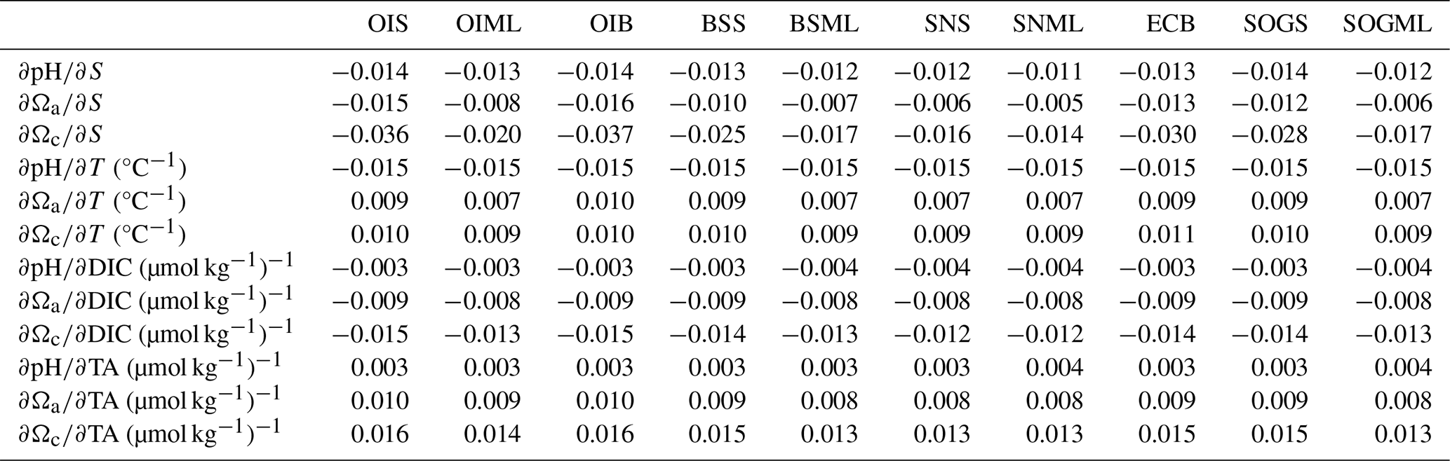
Table A5 Uncertainty in the seasonal mean DIC and TA for each location.

Table A6 Measurement uncertainty of DIC, TA, S, and T.

Table A7 Uncertainties in partial derivatives.

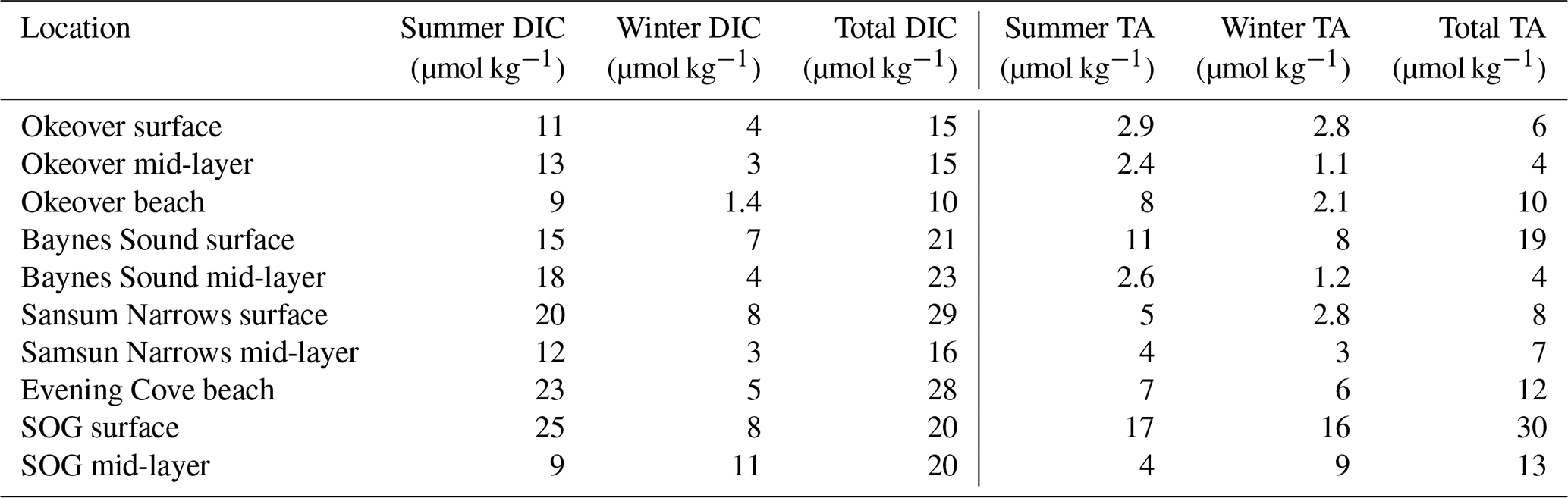
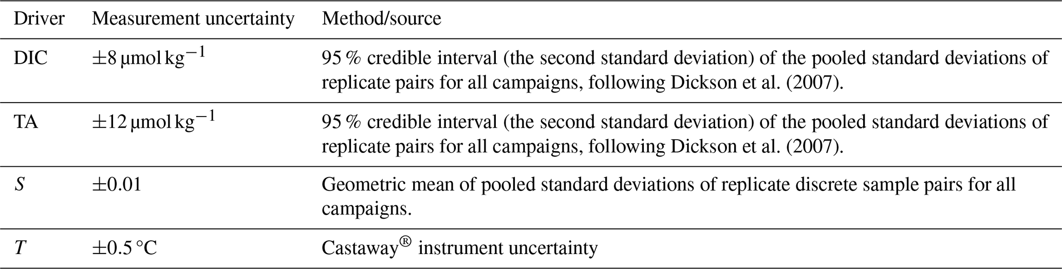
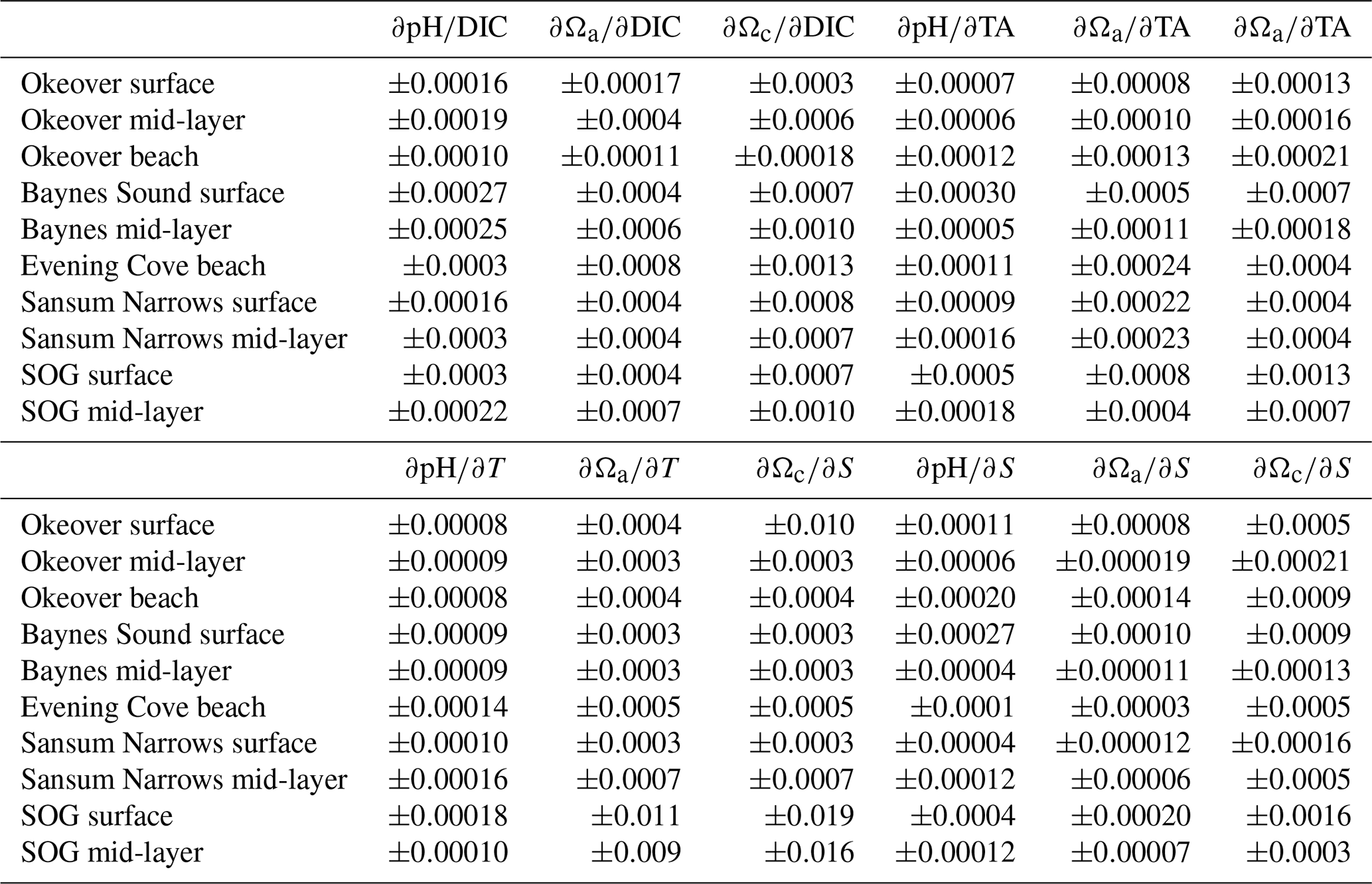
Table A8 Total number of samples taken at each location in the surface and mid-layers.

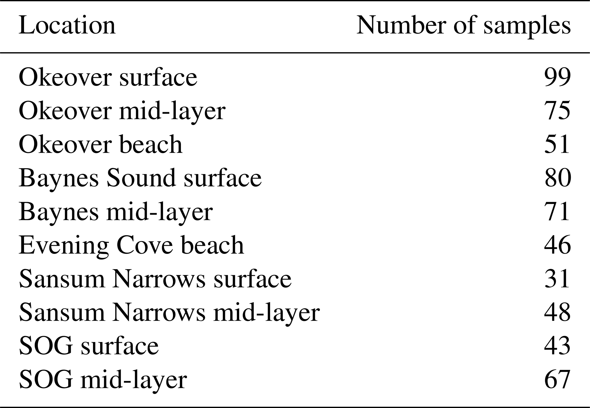
Table A9 Seasonal Taylor expansion results. Contributions to total seasonal changes in pH, Ω_a, and Ω_c from biological changes in DIC ($\frac{\partial \mathrm{pH}}{\partial \mathrm{DIC}}\mathrm{\Delta }{\mathrm{DIC}}_{\stackrel{\mathrm{‾}}{\mathrm{s}}}$) and TA ($\frac{\partial \mathrm{pH}}{\partial \mathrm{TA}}\mathrm{\Delta }{\mathrm{TA}}_{\stackrel{\mathrm{‾}}{\mathrm{s}}}$), T ($\frac{\partial \mathrm{pH}}{\partial T}\mathrm{\Delta }T$), and freshwater ($\frac{\partial \mathrm{pH}}{\partial \mathrm{fw}}\mathrm{\Delta }\mathrm{fw}$). Uncertainties are shown in parentheses. Values greater than uncertainty are highlighted in bold font.

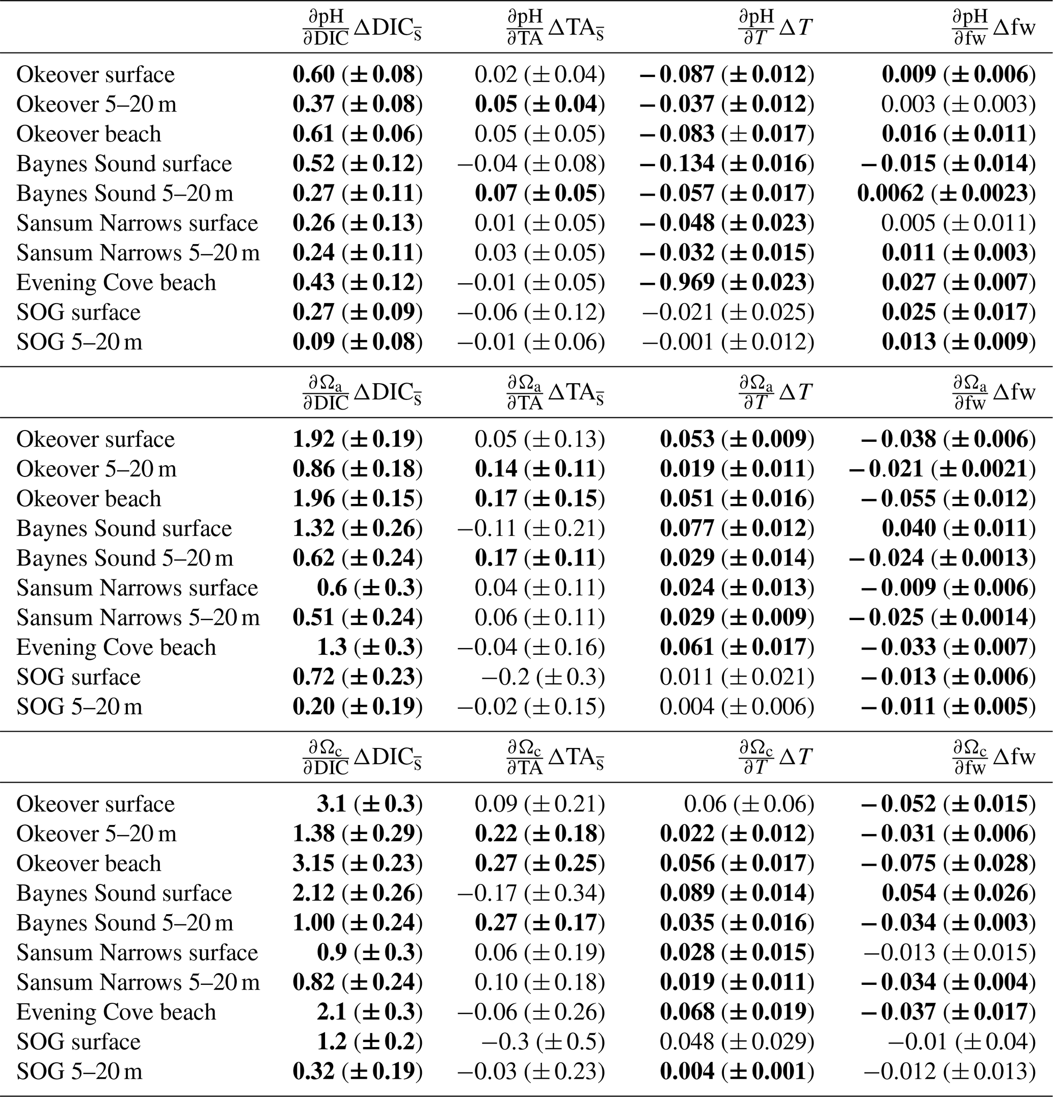
Table A10 Diel Taylor expansion results. Contributions to total diel changes in pH, Ω_a, and Ω_c from biological changes in DIC ($\frac{\partial \mathrm{pH}}{\partial \mathrm{DIC}}\mathrm{\Delta }{\mathrm{DIC}}_{\stackrel{\mathrm{‾}}{\mathrm{s}}}$) and TA ($\frac{\partial \mathrm{pH}}{\partial \mathrm{TA}}\mathrm{\Delta }{\mathrm{TA}}_{\stackrel{\mathrm{‾}}{\mathrm{s}}}$), T ($\frac{\partial \mathrm{pH}}{\partial T}\mathrm{\Delta }T$), and freshwater ($\frac{\partial \mathrm{pH}}{\partial \mathrm{fw}}\mathrm{\Delta }\mathrm{fw}$). Uncertainties are shown in parentheses. Values greater than uncertainty are highlighted in bold font.

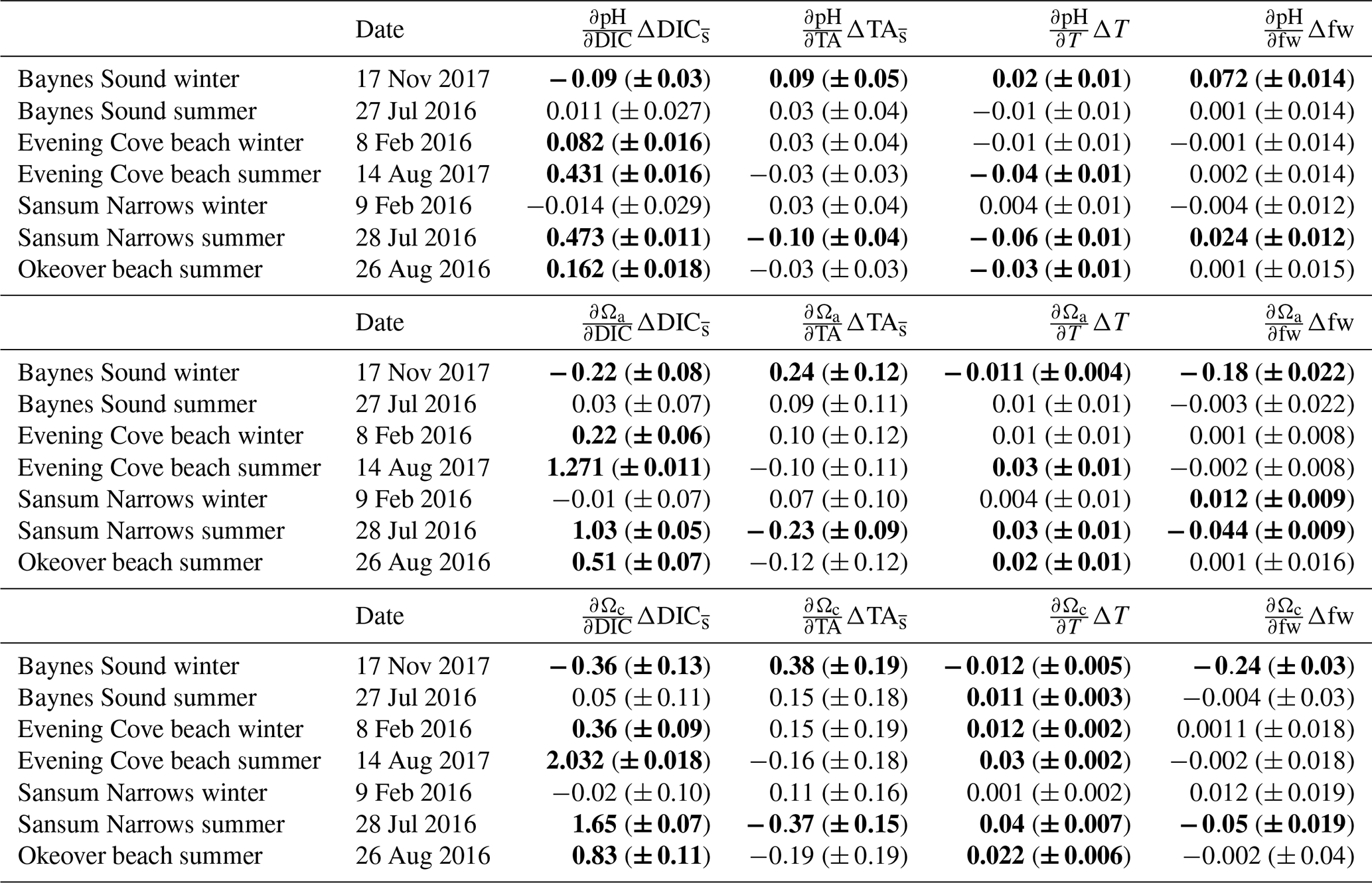
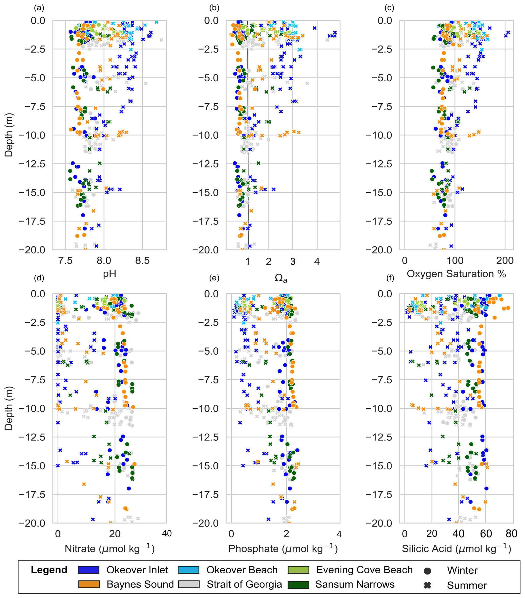
Figure A1 Winter (points) and summer (crosses) depth profiles of observational: (a) pH, (b) Ω_a, (c) oxygen saturation, (d) nitrate concentration, (e) phosphate concentration, and (f) silicic acid concentration, at each nearshore location and the SOG.