the Creative Commons Attribution 4.0 License.
the Creative Commons Attribution 4.0 License.
 | 21 Mar 2024
Non-steady-state stomatal conductance modeling and its implications: from leaf to ecosystem
Yujie Wang
Troy S. Magney
Christian Frankenberg
Accurate and efficient modeling of stomatal conductance (gs) has been a key challenge in vegetation models across scales. Current practice of most land surface models (LSMs) assumes steady-state gs and predicts stomatal responses to environmental cues as immediate jumps between stationary regimes. However, the response of stomata can be orders of magnitude slower than that of photosynthesis and often cannot reach a steady state before the next model time step, even on half-hourly timescales. Here, we implemented a simple dynamic gs model in the vegetation module of an LSM developed within the Climate Modeling Alliance and investigated the potential biases caused by the steady-state assumption from leaf to canopy scales. In comparison with steady-state models, the dynamic model better predicted the coupled temporal response of photosynthesis and stomatal conductance to changes in light intensity using leaf measurements. In ecosystem flux simulations, while the impact of gs hysteresis response may not be substantial in terms of monthly integrated fluxes, our results highlight the importance of considering this effect when quantifying fluxes in the mornings and evenings, as well as interpreting diurnal hysteresis patterns observed in ecosystem fluxes. Simulations also indicate that the biases in the integrated fluxes are more significant when stomata exhibit different speeds for opening and closure. Furthermore, prognostic modeling can bypass the A-Ci iterations required for steady-state simulations and can be robustly run with comparable computational costs. Overall, our study demonstrates the implications of dynamic gs modeling for improving the accuracy and efficiency of LSMs and for advancing our understanding of plant–environment interactions.
- Article
(4248 KB) - Full-text XML
-
Supplement
(693 KB) - BibTeX
- EndNote


Modeling stomatal conductance (gs), the opening and closure of tiny pores on leaves, is one of the key elements and challenges in land surface models (LSMs). Stomata regulate the gas exchange rates of plants, allowing the uptake of CO2 for photosynthetic assimilation while constraining water loss through transpiration (Berry et al., 2010; Damour et al., 2010). The behavior of stomata, especially their responses to environmental variations, plays a significant role in determining the fluxes of carbon, water, and energy between vegetated surfaces and the atmosphere (Berry et al., 2010; Buckley, 2017). Therefore, accurate and efficient modeling of gs is important for understanding the current Earth system and projecting future changes.
Stomatal conductance has been traditionally predicted with empirical models, relating gs to photosynthesis rate and environmental cues with estimated parameters from statistical regressions (Ball et al., 1987; Leuning, 1990, 1995; Medlyn et al., 2011; Damour et al., 2010). Efforts have also been made to constrain stomatal behavior from the principle of optimizing the trade-offs between carbon gain with the related penalty of stomatal opening (Wolf et al., 2016; Venturas et al., 2018; Wang et al., 2020). Additional understanding of stomatal response includes plant hydraulic models that consider the transport of water from soil through plants into the atmosphere (soil–plant–atmosphere continuum, SPAC) (Sperry et al., 1998, 2002; Bonan et al., 2014). However, most existing stomatal models, especially those currently used to scale from leaf to canopy level and implemented in LSMs, assume steady states (Vialet-Chabrand et al., 2017). They predict the opening and closure of stomata in stationary regimes, modeling stomatal response to environmental variations as immediate jumps between states (Vialet-Chabrand et al., 2013).
While steady-state models assume that stomatal conductance changes instantaneously with the environment, the temporal response of stomata in reality can often be an order of magnitude slower than the biochemical response of photosynthesis (Pearcy and Seemann, 1990; Vialet-Chabrand et al., 2013). Plants can experience frequent environmental changes on a timescale of seconds, such as light fluctuations due to cloud cover and canopy shading. Meanwhile, stomatal response times vary from minutes to more than an hour. Thus, a steady state is often not reached when environmental conditions change faster than stomata can respond to (Lawson and Blatt, 2014; Vialet-Chabrand et al., 2017). This slower response of gs could further impose regulations on assimilation rate via its effects on intercellular CO2 concentration (Ci), notably under rapidly changing incident radiation in natural environments (Kaiser and Kappen, 2000; Vialet-Chabrand et al., 2017). The mismatch and interaction of photosynthesis and stomatal response could lead to temporal variations in water use efficiency (WUE) as well (Lawson et al., 2011; Venturas et al., 2018). These can all lead to biases, and it is important to consider non-steady-state temporal responses of gs for more accurate predictions of ecosystem fluxes. Additionally, the inclusion of this factor may also contribute to the hysteresis of plant responses and ecosystem fluxes observed in natural diurnal cycles (Vialet-Chabrand et al., 2013); e.g., evapotranspiration (ET) rates tend to be higher in the afternoon under the same incoming radiation, while canopy conductance overall decreases. These patterns have often been attributed solely to the asymmetry of meteorological variables, especially in temperature and vapor pressure deficit (Zeppel et al., 2004; Bai et al., 2015; Gimenez et al., 2019; Oogathoo et al., 2020; Lin et al., 2019).
The current practice of employing gs models that assume steady states requires iterations to converge to stable solutions at each simulation step. At the leaf level, this typically involves two nested iteration loops: first to solve the coupled photosynthesis–stomatal conductance (An−gs) model for Ci and then to solve the leaf energy budget for leaf temperature (Collatz et al., 1991; Bonan et al., 2018), as gs affects latent heat flux through transpiration. This approach can potentially lead to numerical issues (Sun et al., 2012) and increased computational costs, particularly when upscaling with complex canopies, where angular distribution setups are necessary (Wang and Frankenberg, 2022). However, by utilizing prognostic updates of variables, a dynamic model could simplify simulation steps and improve computational efficiency, enabling runs at finer temporal resolutions.
Moreover, accurate parameter estimation with steady-state models (e.g., linear fitting for the slope g1 in empirical models) necessitates measurements to be taken after reaching each equilibrium (Leuning, 1990; Miner et al., 2017). Depending on wide-ranging stomatal response speeds (McAusland et al., 2016), obtaining one accurate response curve could take several hours (Liozon et al., 2000; Duarte et al., 2016). Too short of a time step could result in overestimation, underestimation, or unstable results of parameter estimates with steady-state assumptions (Xu and Baldocchi, 2003), which may often be overlooked (Miner et al., 2017). Alternatively, estimates can be approached with a prognostic model by fitting the entire response curve, where steady-state measurements are not fundamentally necessary.
Limitations of steady-state stomatal modeling have driven efforts to develop dynamic models, primarily at the leaf level (Damour et al., 2010; Vialet-Chabrand et al., 2017). Based on observed variations of gs, analytical equations of sigmoidal or exponential response have been commonly used (Naumburg and Ellsworth, 2000; Noe and Giersch, 2004; Vialet-Chabrand et al., 2013, 2017; Martins et al., 2016; McAusland et al., 2016); directly adding time-dependent terms to traditional steady-state models has also been proposed (Matthews et al., 2018). While these models have demonstrated effective performance in reproducing leaf-level responses to light intensity in controlled conditions, the impacts of including temporal stomatal dynamics on the simulations of larger-scale fluxes under coupled variations in the natural environment (e.g., transpiration in the coupled diurnal cycles of radiation, temperature, and vapor pressure deficit – VPD) have not been investigated. This may be partly due to the parameterization and complexity of many models optimized for leaf-scale predictions (Kirschbaum et al., 1988; Vialet-Chabrand et al., 2016), which constrains the feasibility of scaling them to the canopy level in LSMs.
In this study, we aim to (1) implement a simplified dynamic stomatal model in the CliMA Land model, i.e., the land component of a new-generation Earth system model within the Climate Modeling Alliance (CliMA); (2) test model performance on leaf-level measurements and demonstrate an alternative method of parameter estimation with the non-steady-state model in a Bayesian nonlinear inversion framework; and (3) compare simulations of the dynamic model with traditional steady-state modeling, primarily focusing on the differences in predictions of canopy fluxes and responses to coupled environmental variations on different timescales.
2.1 Model framework
2.1.1 Dynamic stomatal modeling
The current steady-state modeling approach in LSMs requires convergence of nested iteration loops to solve leaf fluxes at each time step (Fig. 1a) (Bonan et al., 2018). In this study, we proposed replacing the inner loop for steady solutions of the coupled photosynthesis–stomatal conductance (An−gs) model with prognostic updates of gsw at finer time steps (Fig. 1b).
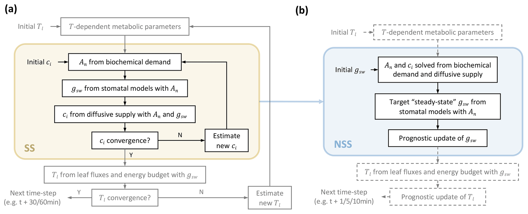
Figure 1Comparison of leaf flux calculation flows in (a) steady-state (SS) and (b) non-steady-state (NSS) dynamic modeling. Panel (a) illustrates the two nested loops at each time step in the current practice of a steady-state framework; adapted from Bonan et al. (2018). The inner iteration in the light yellow box represents the flow of solving the coupled photosynthesis–stomatal conductance (An−gs) model for Ci. The outer one solves the leaf energy budget for leaf temperature (Tl). The focus of this study is to implement and compare a dynamic modeling framework to the An−gs model, illustrated in the light blue box in (b), where, instead of iterating for steady solutions, gsw is updated prognostically at finer time steps based on environmental conditions and a simplified dynamic model (Sect. 2.1.1). This NSS framework of modeling gsw also allows prognostic updates of Tl. As its implementation is not within the scope of this study, related flows are shown in dashed parts.
At each step, instead of assuming an initial Ci and iterating until convergence, our framework starts with an initial gsw (e.g., for the first time step of a diurnal simulation from midnight, this can be set as the minimal conductance in the dark), then solves An and Ci with biochemical demand and diffusive supply of internal CO2 (Fig. 1). For instance, when applying the Farquhar photosynthesis model for C3 plants (Farquhar et al., 1980), with a given gsw, the RuBisCO-limited rate (Ac) and light-limited rate Aj are calculated using
where the middle parts in Eqs. (1) and (2) represent the biochemical demand, and the right part represents the diffusive supply limitation of photosynthesis. Vcmax is the maximum carboxylation rate, Ca is the ambient CO2 concentration, Rd is the respiration rate, Γ* is the CO2 compensation point with the absence of respiration, J is the electron transport rate, Km is the Michaelis–Menten coefficient, and glc is the leaf total conductance to CO2, which can be calculated using , with gbc the boundary conductance to CO2 and gm the mesophyll conductance. Note that computing Ac or Aj requires solving for Ci first. With a known glc from gsw at each time step, rearranging Eqs. (1) and (2) allows for the analytical solution of Ci, Ac, and Aj.
For prognostic updates of gsw, we implemented a simplified dynamic model, adapted from previous studies on leaf-level prognostic modeling (Kirschbaum et al., 1988; Rayment et al., 2000; Noe and Giersch, 2004; Vialet-Chabrand et al., 2016):
where Δt is the time step of the simulation, gt represents the conductance at the current time step, gss is the target conductance calculated with steady-state models at the current conditions, and τ is the time constant, representing the timescale of stomatal responses. In this study, we used the Ball–Berry model (Ball et al., 1987) to compute the gss for leaf-level simulations for simplicity and the Medlyn model (Medlyn et al., 2011) for the canopy-scale simulations, as the vegetation trait dataset (De Kauwe et al., 2015) we employed for our study region is only available for the Medlyn parameters. We should note that the selection of the empirical stomatal model is of minor relevance to our primary findings, as our study focuses on the differences between steady-state and prognostic schemes only.
As indicated in the flowchart (Fig. 1), our dynamic modeling avoids nested iterations for steady solutions while requiring updates of variables at finer time steps (e.g., 5–10 min, compared to 30 or 60 min time steps of current LSMs) for the stability of simulations, which we tested and discuss in Sects. 2.3.2 and 3.3. The prognostic updates of leaf temperature can be implemented accordingly, but as it is not within the scope of this study, we prescribed the leaf temperature updates with measurements in our simulations.
2.1.2 Implementation in LSM
CliMA Land (https://github.com/CliMA/Land, last access: 23 March 2023), a new-generation LSM, is highly modularized and offers flexible model schemes (Wang et al., 2021, 2023), enabling easy implementation and assessment of the dynamic stomatal model across scales. To test the model performance and compare simulations with different stomatal modeling schemes, we implemented our non-steady-state framework in CliMA Land. More information on the CliMA Land configuration can be found in the Supplement (Sect. S1.1) and Wang et al. (2021, 2023).
2.2 Performance on leaf-level measurements
2.2.1 Leaf gas exchange
To test our model and determine key parameters, we recorded light response curves of grape (Vitis vinifera) and walnut (Juglans regia cv.) leaves using an LI-6800 portable photosynthesis system (LI-COR, Inc., Lincoln, NE, USA). Saplings of Vitis vinifera and Juglans regia cv. were planted in 5-gallon (19 L) pots with UC soil mix. 44.4 mL of Osmocote® Smart-Release® Plant Food Plus fertilizer was added to each pot. The plants were grown in a UC Davis lath house. The plants were watered to maintain around 75 % of completely saturated soil by weight (details in Meeker et al., 2021). The youngest, fully expanded, intact leaf was chosen and dark-adapted for 30 min. During the measurements, the photosynthetic photon flux density (PPFD) was sequentially increased following the gradient of 50, 100, 200, 400, 600, 900, 1200, 1500, and 1800 µmol m−2 s−1, with a time step of 30 min at each light level. The chamber air temperature was set at 25 °C; CO2 partial pressure was controlled at 400 ppm, and the relative humidity in the chamber was maintained around 50 %.
2.2.2 Parameter optimization
We applied a Bayesian nonlinear inversion framework (Rodgers, 2000; Dutta et al., 2019) to jointly fit the response curves of the net photosynthetic assimilation (An) and stomatal conductance (gs) for each leaf with the non-steady-state model. The forward problem in this case can be represented as follows:
where y represents the measurements, i.e., the light response curves of both An and gs (see Sect. 2.2.1); ℱ represents the forward model, CliMA Land with the dynamic gs model (see Sect. 2.1); and X is the state vector of parameters to be retrieved, which in our case includes the maximum carboxylation rate (Vcmax), the slope (g1), and the minimum conductance (g0) of the BB model, the mesophyll conductance (gm) (Sun et al., 2014), and the time constant (τ). We also included a scaling factor for An to account for variations in the respiration rate and the ratios between CO2 and H2O fluxes; b is the vector of other parameters that have influences on the measurements and are known to some accuracy but not intended to be retrieved, e.g., the ratio between Jmax (the maximum electron transport rate) and Vcmax, which is assumed to be 1.6 in this study but may vary across conditions (Medlyn et al., 2002), and ϵ is the error term.
The Levenberg–Marquardt (LM) iterations (Levenberg, 1944; Marquardt, 1963; Rodgers, 2000) were utilized to solve the nonlinear inversion problem and find the best estimate of key parameters:
where xa is the prior estimate of the state (in this study, Vcmax: 70 µmol m−2 s−1, g1: 9, g0: 0.03 mol H2O m−2 s−1, gm: 0.4 mol CO2 m−2 s−1, τ: 600 s, scalingA: 1), and Sa is the prior covariance matrix, assumed to be purely diagonal, with Gaussian uncertainties in the prior state (the assumed prior standard deviation of Vcmax: 30, g1: 3, g0: 0.005, gm: 0.02, τ: 100, scalingA, 0.01). Ki is the Jacobian matrix at the ith iteration. γ is adjusted at each step, ensuring that each update of the state vector moves towards minimizing the cost function. Sϵ is the error covariance matrix; in our case, errors were assumed to be mainly from measurement uncertainties and calculated based on the standard deviation and mean of the ΔCO2 and ΔH2O in LI-6800 measurements.
2.2.3 Uncertainties in traditional parameter estimation
To illustrate the influence of time steps on parameter estimation in the traditional method, which assumes steady states, we used the NSS model to generate leaf response curves to the same PPFD sequence but with different time intervals. For example, in the 5 min time step simulation, light intensity input jumped every 5 min, and measurements were assumed to be taken right before the next jump, following the traditional method. We then employed these curves to calculate the estimated g1 and g0 values using the traditional linear fitting method for the Ball–Berry model. The potential biases were assessed by comparing fitted parameters with different applied time steps.
2.3 Comparison of models in diurnal cycles
To assess the potential bias of the current steady-state modeling in LSMs, we compared the predictions of surface fluxes from models with different assumptions under natural environmental variations. We evaluated and compared the simulation results on both the leaf and canopy flux scales.
2.3.1 Environmental drivers and plant traits
As the light intensity tends to be the most rapidly changing environmental condition that stomata response to, we employed high-temporal-resolution radiation measurements in the field as the incoming irradiance inputs and ran CliMA Land with both setups. Photosynthetically active radiation (PAR) in a crop field (42.481677° N, 93.523521° W) was recorded with an LI-190R quantum sensor (LI-COR, Inc., Lincoln, NE, USA) at 1 s temporal resolution during August 2017.
In addition to the fluctuations of total incoming photon density that the PAR sensor can provide, canopies in natural environments also experience variations in the fraction of direct and diffuse components in the total radiation. This variation affects the distribution of PAR received by individual leaves across different layers of the canopy structure (Durand et al., 2021). To account for this effect, we employed an empirical fitting with the hourly radiation data from ERA5 (Fig. S2 in the Supplement) to estimate the partitioning between the direct and diffuse radiation (Boland et al., 2001). The empirical relationship was then applied to high-temporal-resolution PAR measurements to obtain the direct and diffuse components in the recorded total radiation, which were used as inputs for simulations at the canopy scale.
Other meteorological variables (e.g., air temperature, dew-point temperature, volumetric soil water, wind speed) were extracted from the ERA5 hourly reanalysis dataset (Hersbach et al., 2018) and input as environmental drivers for the simulations on the canopy scale. Linear interpolations were applied for runs at sub-hourly time steps. Key plant traits (e.g., Vcmax, g1, leaf area index – LAI) were extracted from several globally gridded datasets using GriddingMachine (Wang et al., 2022; Croft et al., 2020; Butler et al., 2017; Luo et al., 2021; De Kauwe et al., 2015; Yuan et al., 2011; He et al., 2012; see also Wang et al., 2023, for detailed information on global-scale datasets used in CliMA Land).
2.3.2 Model simulations
We ran the CliMA Land surface flux simulations with different stomatal modeling schemes to assess the effects of gs temporal response on model predictions. In the SS runs, iterations were employed to converge to steady-state solutions at each time step. For NSS mode, previous studies have observed different time constants for stomatal opening (τop) and closure (τcl) in various species, as well as a positive correlation between τop and τcl, with the ratio varying from around to 3 (McAusland et al., 2016; Vico et al., 2011; Ozeki et al., 2022). Based on the average time constant retrieved from the leaf response curves in Sect. 2.2.1 and 2.2.2 as well as previous estimates of the time constant variations (Vialet-Chabrand et al., 2013; McAusland et al., 2016; Vialet-Chabrand et al., 2017; Vico et al., 2011; Ozeki et al., 2022), we tested several sets of τop and τcl varying from 300 to 900 s, including (a) s, as the base comparison; (b) τop>τcl, with ratios varying from 1.2 to 3, e.g., τop = 900 s, τcl=300 s; and (c) τcl>τop, with ratios from 1.2 to 3, e.g., τop=300 s, τcl=900 s.
For the leaf-scale runs, we used the key parameters retrieved in previous sections and tested model predictions for an ideal clear-sky day. To investigate the differences in ecosystem fluxes, we ran and assessed the NSS and SS simulations using a time step of 1 min, with the inputs of meteorological drivers and plant traits at the location of the PAR measurement for the month of August 2017. Meteorological variables are updated at each time step. In order to further evaluate the potential contribution of gs hysteresis to the observed diurnal hysteresis of ecosystem fluxes, we compared the standard runs with the model predictions where environmental variables (e.g., temperature, VPD, soil water content – SWC) were held constant over the daytime (as the mean of daytime values in each day). This approach allowed us to isolate the effect of hysteresis in gs response and assess its potential contribution to the observed diurnal hysteresis of canopy and ecosystem fluxes.
Furthermore, to test the stability of prognostic modeling and assess the computational cost, we compared NSS simulations using different time steps, as well as the SS simulation run at a time step of 30 min, which is commonly used in current LSMs. This enabled us to evaluate the sensitivity of NSS predictions to the time step used, as well as to compare the computational cost for stable NSS runs and standard SS simulations. We resampled the environmental drivers from ERA5 and the PAR sensor to match the temporal resolution of the simulations, while maintaining constant average values for each diurnal cycle across simulations with different time steps.
3.1 Model performance and parameter estimates on leaf measurements
With the parameters estimated from the LM inversion framework, the non-steady-state model predicted the temporal responses of gsw and An well (Fig. 2). The model was able to capture the gradual increases in gsw and An after each step change in APAR, and the reproduced curves were close to the measurements, with all R2 higher than 0.98. Fitted time constant τ showed a variation between the two example leaves (292 and 2028 s for the Vitis vinifera leaf and the Juglans regia cv. leaf, respectively). The relative difference in the time constant matched the variations of response speed observed in the measured response curves (Fig. 2). Compared to the SS model, the dynamic model provided more accurate prediction of the temporal responses. The improvements in R2 were more prominent in the predictions of the Juglans regia cv. leaf responses, which have a larger time constant, than in those of the Vitis vinifera leaf. Other parameters estimated for the Vitis vinifera leaf include Vcmax of 71 µmol m−2 s−1, g1 of 11.3, g0 of 0.023 mol H2O m−2 s−1, gm of 0.18 mol CO2 m−2 s−1, and scalingA of 1.1. For the Juglans regia cv. leaf, Vcmax is 152 µmol m−2 s−1, g1 is 3.9, g0 is 0.052 mol H2O m−2 s−1, gm is 0.34 mol CO2 m−2 s−1, and scalingA is 1.0.
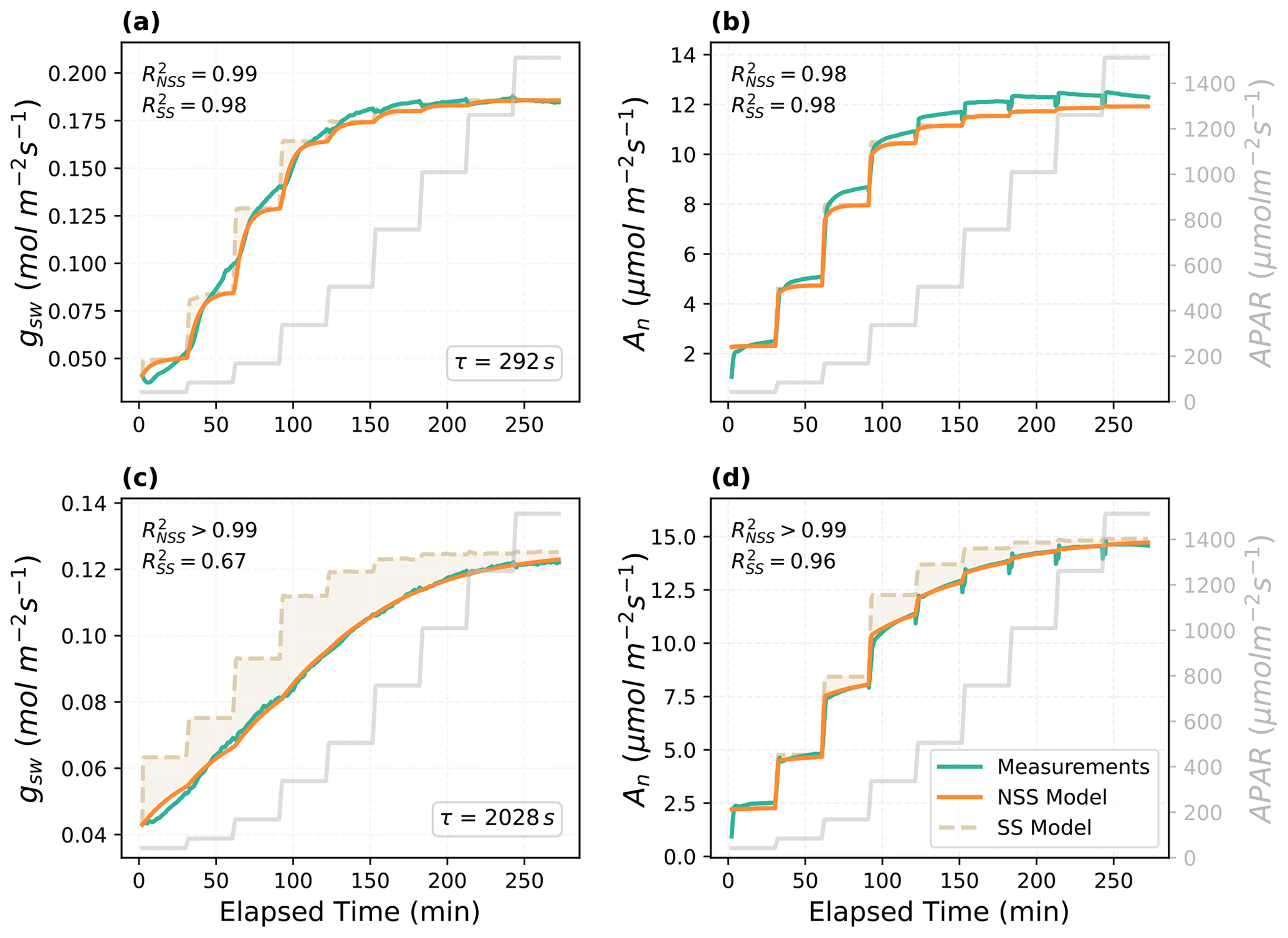
Figure 2Modeled and measured temporal responses of the stomatal conductance (gsw) and net photosynthesis rate (An) to the step changes in APAR for different leaves. The shaded area indicates the difference between the prediction of the steady-state (SS) model and the non-steady-state (NSS) dynamic model. (a–b) The temporal responses of the Vitis vinifera leaf and (c–d) the Juglans regia cv. leaf.
The dynamic model was also able to better capture the temporal variations of internal CO2 concentration (Fig. 3). Particularly, the NSS model reproduced the undershooting of the intercellular CO2 concentration (Ci) after each step change in light intensity, which resulted from the differences in the speed of gs and An responses and their interactions. As shown in the measured time series (Fig. 2), after each increase in the incident light, photosynthesis was able to respond almost instantaneously, leading to a rapid decrease in Ci, while stomata opened gradually, slowly bringing up Ci over time. This then led to a gradual rise of An after the initial rapid response, indicating the regulation of gs on An through its impacts on the internal CO2 supply. In the meantime, the increasing An further promoted the opening of stomata with a higher internal CO2 demand, demonstrating their coupled responses to environmental variations.
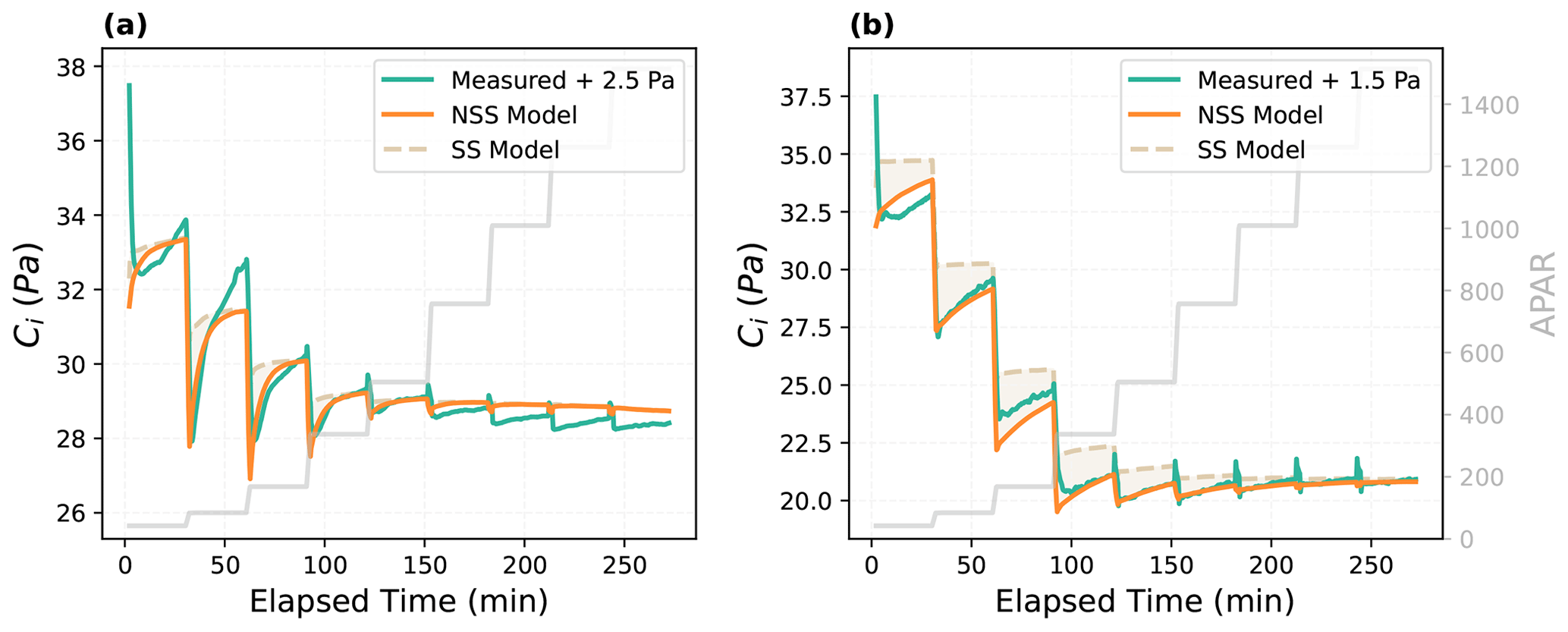
Figure 3Modeled and measured temporal responses of intercellular CO2 concentration (Ci) for (a) the Vitis vinifera leaf and (b) the Juglans regia cv. leaf. As indicated by the labels, measured curves were shifted to illustrate the comparison of modeled and measured response patterns, as the absolute values are not directly comparable due to different assumptions of LI-6800 and CliMA Land in calculating the internal CO2. The shaded area indicates the difference between the prediction of the steady-state (SS) model and the non-steady-state (NSS) dynamic model.
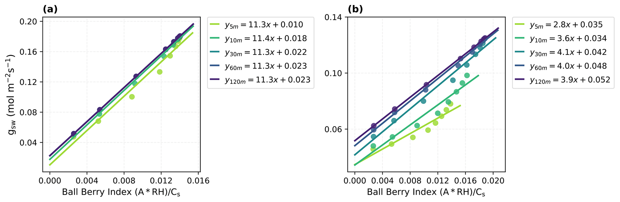
Figure 4Parameter estimates for the Ball–Berry model with the traditional linear fitting method using model-reproduced response curves with different time steps (5, 10, 30, 60, 120 min). (a) Fitting results for the Vitis vinifera leaf and (b) the Juglans regia cv. leaf. Corresponding Ball–Berry index and gsw are plotted, along with the fitted lines and parameters (i.e., the Ball–Berry slope, g1, and the intercept, namely, the minimum conductance, g0).
With the dynamic model and optimized parameters that accurately reproduced the measured leaf responses, we investigated the influence of time steps used in light response curves (i.e., the length of intervals between step changes in light intensity) on parameter estimates obtained with traditional methods (Fig. 4). The results showed that, particularly for the Juglans regia cv. leaf that has a long time constant over 2000 s, the values and relationship between the Ball–Berry index and gsw varied significantly depending on the time step used, resulting in notable uncertainties in fitted g1 and g0 with too short of a interval to reach equilibrium. This also suggested that obtaining reliable estimates for this leaf using the traditional method could require more than an hour for stable readings at each step.
3.2 Model comparison in diurnal cycles
3.2.1 Leaf responses
To compare NSS and SS models over the course of a day, we evaluated the differences in their predictions of leaf responses to an ideal diurnal cycle of light with other environmental conditions (e.g., temperature, VPD, CO2) held constant (Fig. 5). Results showed that compared to NSS, the SS model predicted a higher An and gs in the morning, as it assumed the stomata could respond immediately to an increase in light, while in the more realistic NSS simulation, the gradual opening of stomata limited the CO2 supply for photosynthesis with a lower Ci. The opposite was true for the afternoon, but the overestimation of An and gs in SS modeling in the morning was more significant than the underestimation in the afternoon, leading to slightly higher diurnally integrated predictions than those of the NSS model. This was due to the fact that in the course of sunset, the major limiting factor on productivity was the decreasing light, in contrast to the sunrise where it was the available Ci regulated by gs responses that mainly constrained An increases. The relative differences (RDs) in integrated gs in the morning and afternoon were both higher than those of the photosynthesis, reflecting the differences in the response speed.
The differences in predictions of An and gsw responses also led to RDs in the intrinsic water use efficiency (WUE, i.e., the ratio between An and gsw). Although the mean instantaneous WUE during the daytime was higher in the NSS simulation, diurnal WUE calculated from the integrated An and gsw was lower. This was because the gradual opening of stomata during sunrise limited assimilation in the morning, whereas during sunset, delayed closure led to unnecessary water loss when carbon gain was constrained by low light.
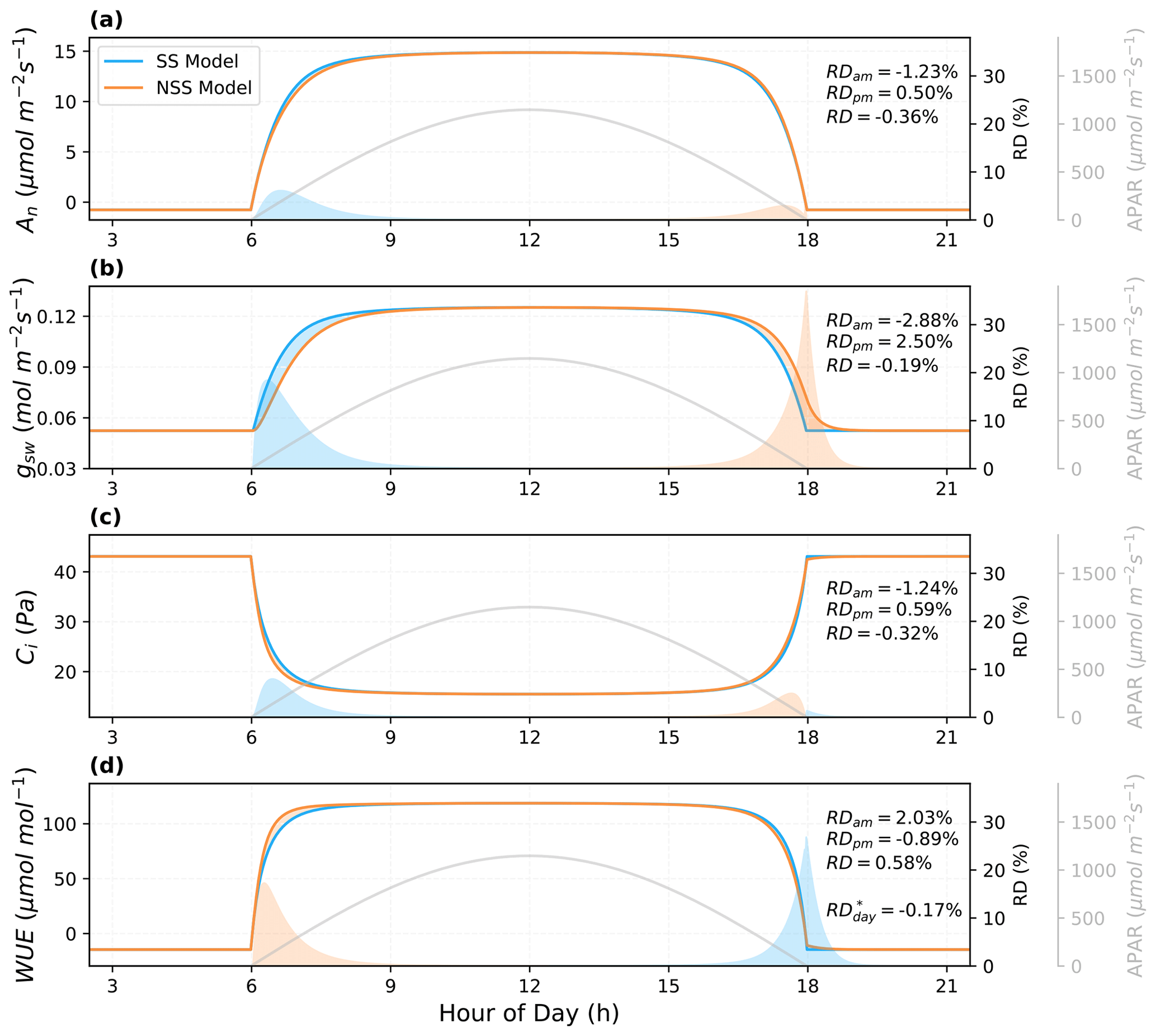
Figure 5Predictions of the leaf diurnal course of (a) net photosynthesis rate (An), (b) stomatal conductance to water vapor (gsw), (c) intercellular CO2 concentration (Ci), and (d) intrinsic water use efficiency (WUE) for a leaf with a stomatal time constant of 900 s on an ideal clear-sky day ( s). Other environmental conditions (e.g., leaf temperature, VPD) were held constant. The shaded areas indicate the differences between the NSS and SS simulations (blue: SS > NSS; orange: SS < NSS) in both absolute and relative terms. Relative differences (RD, NSS − SS) in the temporal integrals are also presented for morning (05:00–12:00 local solar time), afternoon (12:00–19:00), and daytime (05:00–19:00). RD* of WUE represents the ratio between integrated An and gsw, differing from the RD, the integral of the instantaneous WUE during the daytime.
3.2.2 Canopy fluxes
To quantify the impacts of the inclusion of gs temporal response, we analyzed the simulated canopy fluxes under natural radiation variations and coupled dynamics of environmental conditions. As shown in the examples of diurnal cycle simulations (Figs. 6 and 7), the SS model predicted higher variations in instantaneous fluxes in response to rapid fluctuations in radiation, particularly in transpiration rates.
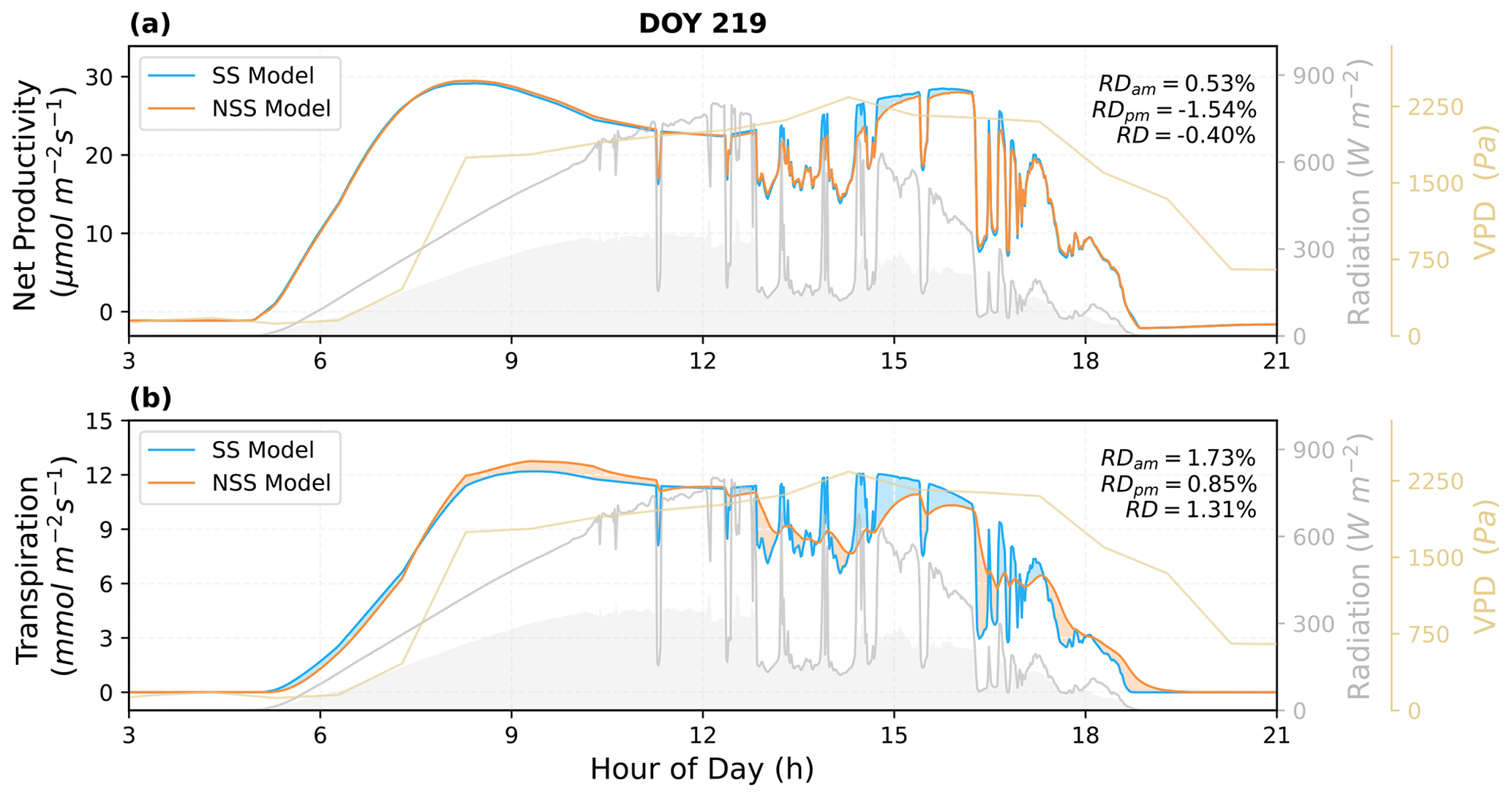
Figure 6Comparison of the predicted diurnal cycles of ecosystem fluxes, as well as (a) the net productivity and (b) the transpiration rate for DOY 219 in 2017. The shaded areas in blue and orange indicate the differences between the NSS and SS predictions (blue: SS > NSS; orange: SS < NSS). The shaded areas in gray under the radiation curves represent the diffuse component of the total radiation. Relative differences (RD, NSS − SS) in the temporal integrated fluxes are also presented for morning (05:00–12:00), afternoon (12:00–19:00), and daytime (05:00–19:00).
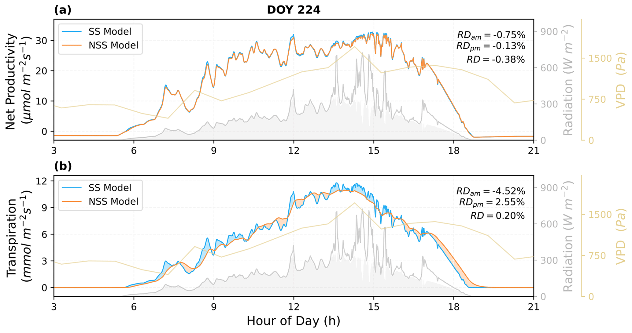
Figure 7Comparison of the predicted diurnal cycles of ecosystem fluxes, as well as (a) the net productivity and (b) the transpiration rate for DOY 224 in 2017. The shaded areas in blue and orange indicate the differences between the NSS and SS predictions (blue: SS > NSS; orange: SS < NSS). The shaded areas in gray under the radiation curves represent the diffuse component of the total radiation. Relative differences (RD, NSS − SS) in the temporal integrated fluxes are also presented for morning (05:00–12:00), afternoon (12:00–19:00), and daytime (05:00–19:00).
When τop=τcl, the overestimate of morning gsw in SS predictions was mostly compensated for by an underestimate of afternoon gsw, resulting in relatively minor differences in daily average gsw (Fig. 8c; the mean RD of daytime mean gsw was 0.5 %). However, when the time constants of stomatal opening and closure were not equal, there was overall underestimation or overestimation in both mornings and afternoons, and the daily mean RDs could be notable (Figs. 8g and k, S3, S4). For example, when τop=3τcl, the faster closure than opening of stomata led to overall lower conductance over the diurnal cycles compared to SS runs (Fig. 8k; the mean RD of daytime mean gsw was −6.1 %).
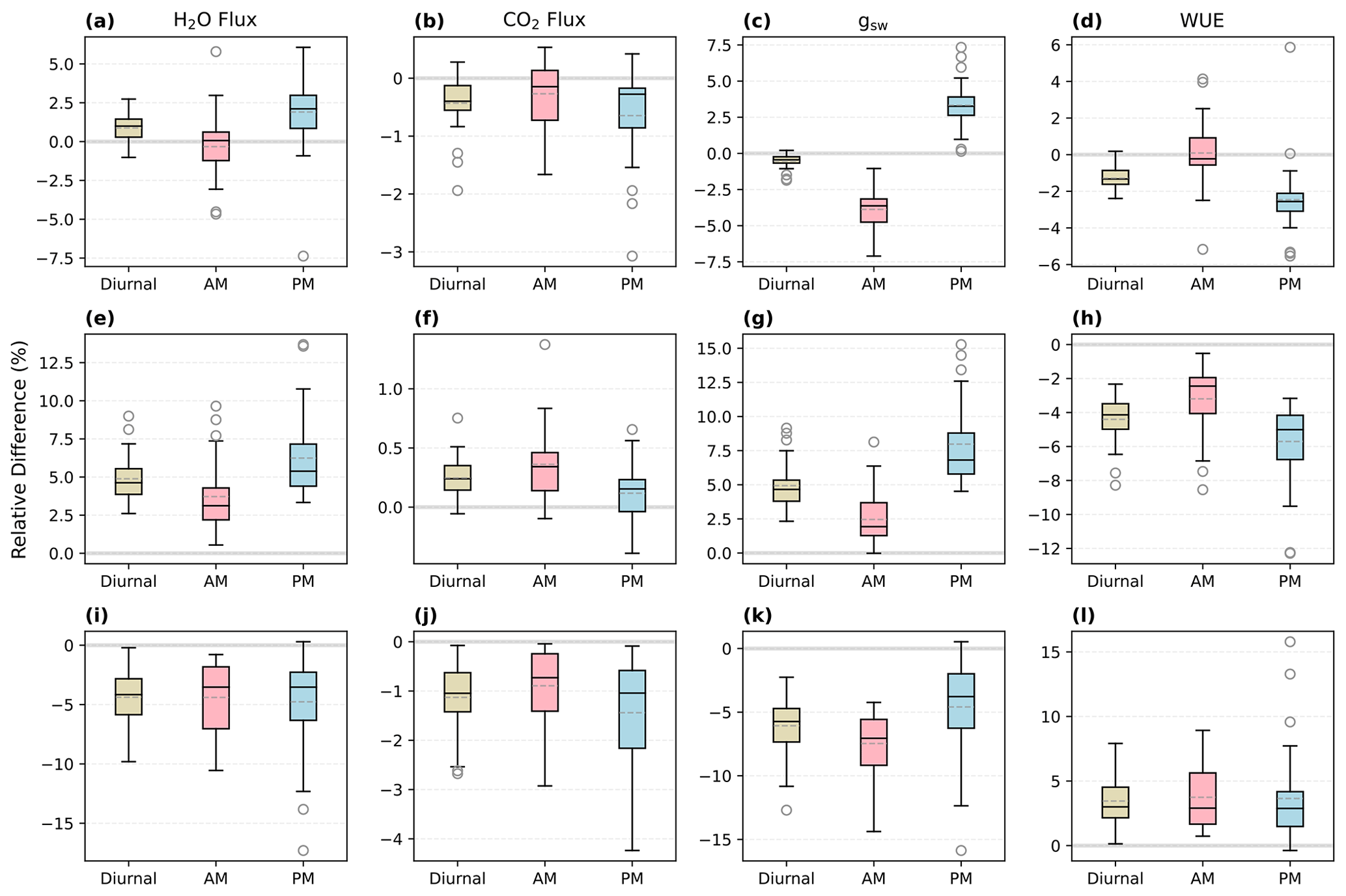
Figure 8Relative differences (NSS − SS; RD) in the predicted daytime mean fluxes of the NSS (time step: 1 min) and SS (1 min) simulations for August 2017. The solid line in each box indicates the median, and the dashed line represents the mean. The results for the transpiration rate (H2O flux), net productivity (CO2 flux), canopy-averaged stomatal conductance to water (gsw), and water use efficiency (WUE) are shown in the respective columns from left to right. (a–d) s, (e–h) τop=300 s, τcl=900 s, (i–l) τop=900 s, τcl=300 s. Diurnal: 05:00–19:00, morning: 05:00–12:00, afternoon: 12:00–19:00.
In the simulations with the same time constants of stomata opening and closure, the differences in fluxes between the NSS and SS predictions were not significant when integrated over monthly periods (e.g., the mean RD of transpiration in August 2017 was 0.87 %, and the median was 1.0 %) but could be notable at sub-diurnal scales depending on the environmental conditions (e.g., the variation of afternoon RDs ranged from −7.4 % to 6.1 %). When there were differences in τop and τcl, the divergences between NSS and SS predictions could be more significant (e.g., when , the mean RD of transpiration in August 2017 was 4.9 %, and the maximum daily mean RD of transpiration was 9.0 %).
The overall tendency to overestimate productivity with traditional SS models was also observed at the canopy scale, when τop was equal to or larger than τcl, as the regulation of gs hysteresis on the supply of CO2 for photosynthesis was not considered (Fig. 8b and j). For example, in Fig. 6, when rapid spikes of radiation occurred in the afternoon, the speed of gs response constrained the increases in photosynthesis in the NSS simulation. However, when τop was smaller than τcl, predicted daily mean photosynthesis was slightly higher in the NSS simulation (Fig. 8f; the mean RD of productivity in August 2017 was 0.2 %). This resulted from the overall higher gsw due to faster opening than closure (Fig. 8g), as higher conductance resulted in higher Ci (Fig. S5), leading to generally higher rates of photosynthesis.
In contrast to the leaf-scale results, when accounting for other covarying environmental drivers (e.g., temperature, VPD, soil water content), the SS model tended to underestimate canopy transpiration rates when τop=τcl (Figs. 6b, 7b, 8a). This could be because the transpiration rates were determined by both gsw and VPD. During the daytime, VPD typically increased following air temperature and peaked in the afternoon, when the slow response of stomata to the increasing VPD and decreasing radiation could result in excess water loss (Figs. 7b, 8a and c). The overestimation of productivity and underestimation of transpiration in SS simulations both contributed to the overestimation of WUE. When τop<τcl, slower stomatal closure led to increased water loss and thus a more significant underestimation of transpiration in the SS predictions (Fig. 8e; the mean RD of transpiration in August 2017 was 4.9 %), resulting in further overestimation of the WUE. When τop>τcl, the NSS model predicted lower transpiration rates and higher WUE compared to the SS model because of the overall lower gsw (Fig. 8i and k). As lower gsw yielded overall lower Ci (Fig. S5), larger gradients of CO2 concentration across stomata contributed to higher WUE on daily and monthly timescales.
3.2.3 Diurnal hysteresis
To investigate the relative contributions of gs hysteresis and environmental variables to the hysteresis observed in plant behaviors and ecosystem fluxes, we separated the effects of these two factors by comparing predicted response curves in NSS and SS simulations with and without diurnal environmental variations (e.g., temperature, VPD, soil water content). While the asymmetry of environmental variables in the diurnal cycle could lead to a modeled hysteresis of gs in response to radiation, where gs tended to be lower in the afternoon mainly due to higher VPD and temperature, our results (Fig. 9) showed that the kinetic lag of gs could partially offset this effect (Fig. 9b and d), even presenting an opposite tendency at low radiation. Additionally, only the NSS model simulations predicted a hysteresis of canopy transpiration, with or without the consideration of coupled environmental variations (Fig. 9g and h), in which canopy H2O fluxes tended to be higher in the afternoon. Differences between τop and τcl affected the magnitudes of hysteresis, but the overall patterns remained similar (Figs. S6, S7).
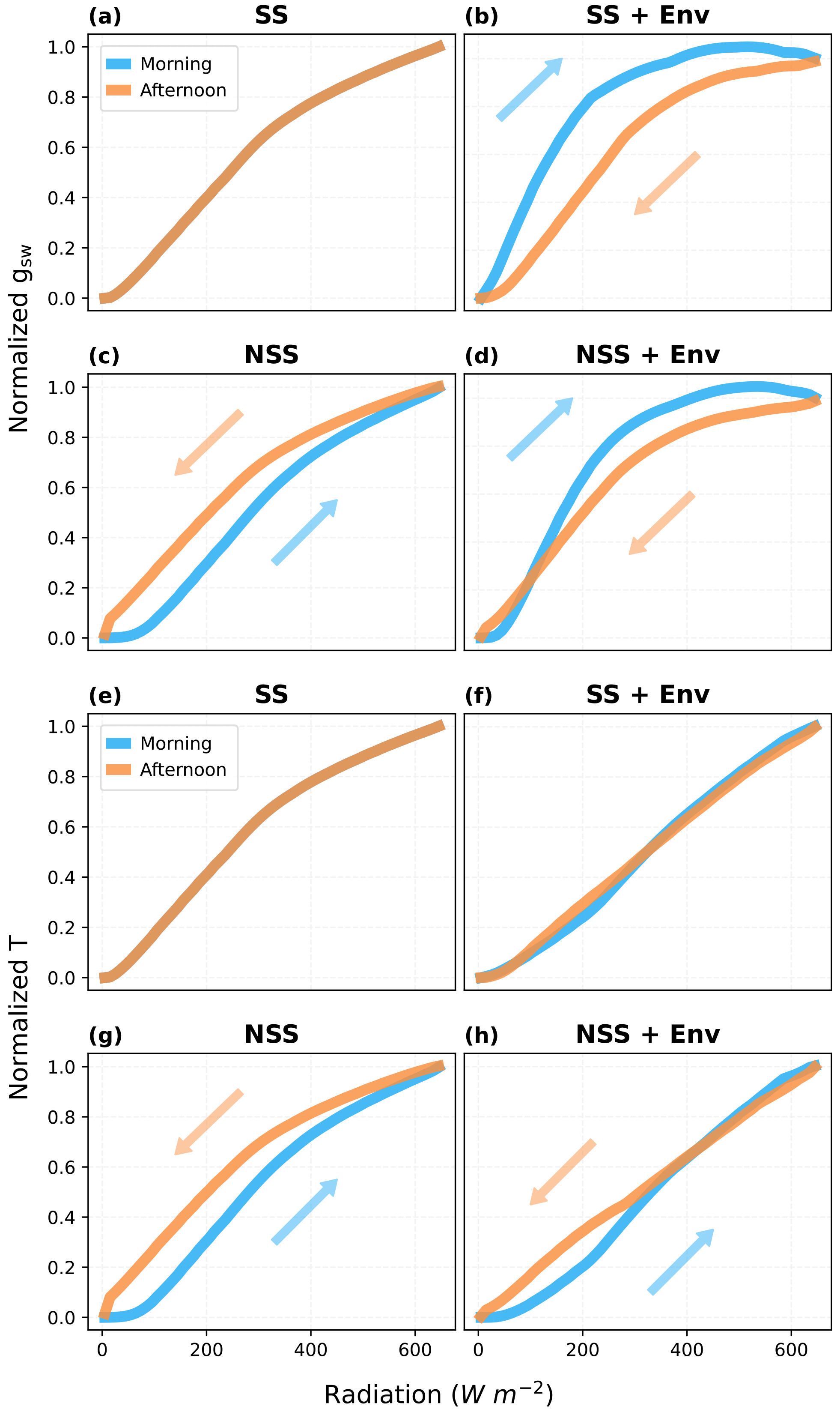
Figure 9Hysteresis of the canopy mean stomatal conductance (gsw) and canopy transpiration rate (T) in response to radiation during an ideal clear-sky day, when s. (a, e) SS model and (b, f) SS model with coupled diurnal variations of environmental conditions (Env, e.g., air temperature, VPD). (c, g) NSS model and (d, h) NSS model with Env. (a–d) Normalized gsw responses and (e–h) normalized T responses. In simulations without Env variations, except for the radiation, all the other environmental drivers were kept at the daytime means. gsw and T are normalized with the values at noon (12:00). Arrows indicate the increasing and decreasing parts of the diurnal courses.
3.3 Stability of the dynamic model
We further assessed the sensitivity of the dynamic modeling to the time step of simulation. Figure 10 shows that the NSS model was be able to run at a time step of 10 min stably and still demonstrated the impacts of gradual gs responses compared to the traditional practice of SS modeling at a time step of 30 min.
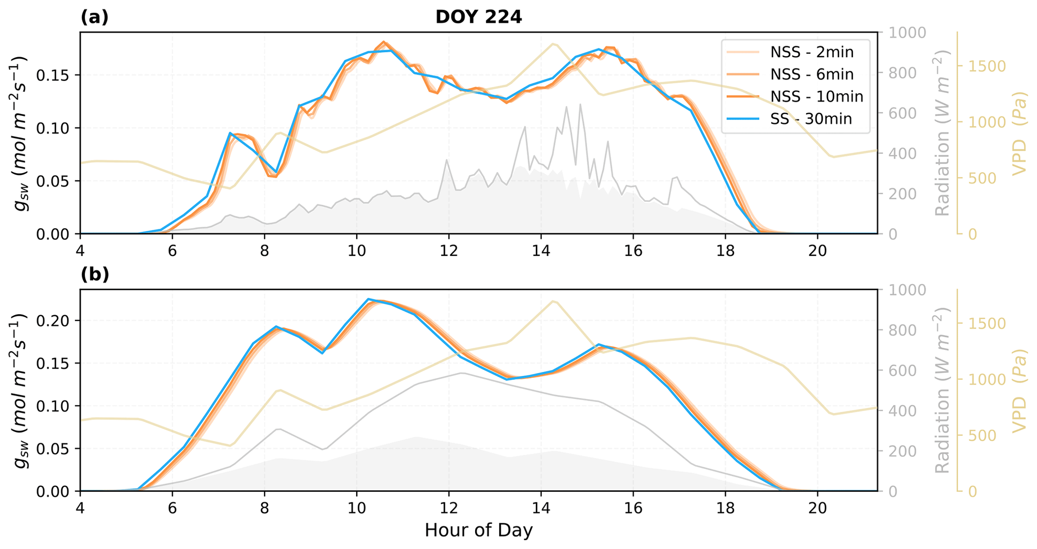
Figure 10Simulations of dynamic gsw using different time steps (2, 6, 10 min) and comparison with the traditional steady-state modeling (30 min resolution) predictions. (a) Using high-temporal-resolution PAR as radiation input, values are resampled accordingly to match the time step used; (b) using ERA5 hourly radiation as input, values are linearly interpolated to 30 min resolution. The shaded areas in gray under the radiation curves represent the diffuse component of the total radiation.
In this study, we demonstrated the feasibility and benefits of implementing a non-steady-state stomatal conductance modeling framework from the leaf to canopy scale in a new-generation LSM, CliMA Land. Our results suggested that compared to traditional steady-state models, the dynamic model was able to provide more realistic and accurate predictions of leaf temporal responses to the changes in light intensity (Sect. 3.1). In the meantime, modeling gs with prognostic updates – similar to how plants control their stomata movements gradually in natural environments – increased neither computational cost nor model complexity, as simulations were simplified with iterations to solve for steady states avoided. Sun et al. (2012) pointed out that the default three-step fix-point iteration for solving the coupled An−gs model in CLM4 (the Community Land Model version 4) does not always converge, leading to uncertainties in flux predictions. In our simulations at the canopy scale (Sect. 3.3), the dynamic model could be stably run at a temporal resolution (10 min) that presented comparable efficiency to the current practice of 30 min resolution SS simulations commonly used in LSMs (three-step prognostic updates for each SS default three-step iteration). This also indicates that the dynamic model can enable predictions of canopy flux dynamics at a finer time resolution with higher efficiency and accuracy.
With the non-steady-state model, we were able to apply a Bayesian nonlinear inversion framework to jointly fit the light response curves of both An and gs and obtain estimates for key parameters (Sect. 3.1). As suggested in our results (Fig. 4) and previous studies (Xu and Baldocchi, 2003; Miner et al., 2017), the time step of light response curves can notably influence the estimated parameters obtained from the traditional linear fitting method for steady-state empirical models. Our framework with the dynamic model can help reduce the time required for accurate parameter estimations, particularly for leaves with long time constants, as equilibrium is not required. Although the retrieval setups presented in this study may not be optimal for estimating Vcmax, which is typically derived from A−Ci response curves (Medlyn et al., 2002; Miao et al., 2009; Duarte et al., 2016), a similar framework can be applied to other scenarios for estimation of various parameters, including an A−Ci curve for Vcmax.
Furthermore, we evaluated how the inclusion of gs temporal responses could affect model predictions of leaf and canopy fluxes in diurnal cycles with natural environmental variations (Sect. 3.2.2). The comparison of NSS and SS simulations indicated that the differences in fluxes depended on the integration timescales, relative speed of stomatal opening and closure, and environmental variations. In terms of instantaneous effects, slow opening of stomata tended to limit productivity responses to rapid radiation increases, and delayed closure of gs following decreases in radiation or increases in environmental stress (e.g., increasing VPD) resulted in unnecessary water loss. The divergence of NSS and SS schemes was less significant when considering the monthly integrated canopy fluxes compared to daily or sub-diurnal-scale results. The monthly differences were more notable when the speeds of stomata opening and closure differed. The overall effects on WUE also depended on the relative speed of opening and closure. In the simulations where stomata open at a speed similar to or faster than they close, excessive water loss in the afternoons, when VPD was high, led to a lower WUE. This also suggested that traditional steady-state simulations may overestimate WUE. Similar impacts have been noted in studies on leaf-scale response to PPFD fluctuations (Lawson et al., 2011; Lawson and Blatt, 2014; McAusland et al., 2016). Meanwhile, when stomata opened more slowly than they closed, plants exhibited both a lower maximum gs during diurnal cycles and a lower average gs compared to the SS runs. This resulted in reduced transpiration and increased WUE, even though productivity was also suppressed. These results suggest that the temporal hysteresis of gs can have impacts on integrated canopy fluxes, and further studies on variations of stomata opening and closure speeds across plants can be helpful to assess these effects more comprehensively on larger scales.
In addition, the hysteresis of leaf-level gs response can contribute to the hysteresis patterns at the ecosystem scale, which have often been solely attributed to the asymmetry of environmental variables during the daytime. For instance, higher evapotranspiration (ET) fluxes and sap velocity (i.e., an indicator of plant transpiration rate) have been observed in the field, with the explanation often focused on higher VPD in the afternoon following increased air temperature (Zeppel et al., 2004; Gimenez et al., 2019; Oogathoo et al., 2020; Lin et al., 2019). Our simulations showed that the SS model with diurnal environmental variations was unable to reproduce this hysteresis pattern, while it was captured in NSS runs. This indicated the significance of considering gs temporal dynamics when interpreting diurnal hysteresis in transpiration (Sect. 3.2.3). Moreover, observed patterns of lower gs in the afternoon have also been commonly explained by similar environmental asymmetry (Bai et al., 2015; Lin et al., 2019), while our results suggested the kinetic lag of gs could partially offset this effect and should thus be taken into account in understanding the hysteresis patterns.
Our study mainly focused on taking the first step to implement prognostic stomatal modeling in an LSM, including the impacts on canopy flux simulations. Further improvements can be made in assessing other effects of gs temporal responses in LSM projections, as well as validating the comparisons with site-level observations. For example, while daily effects on canopy productivity were minor, they may add up to significant differences in long-term vegetation growth trajectories. As plant traits were prescribed in our simulations, the accumulative effects were not included in our analysis of the short-term predictions. The transient limitation on photosynthesis from the slow temporal response of gs could also cause potential photoinhibitory damage to the photosystem II reaction centers. Future studies can focus on the parameterization of these impacts in LSMs and the evaluation of cumulative effects on plant growth and hydraulics in the long term.
The dynamic gs model enables predictions of temporal changes in latent heat flux through transpiration in leaf energy balance, which allows a similar prognostic framework to be employed for the modeling of leaf temperature. Coupled dynamic modeling of stomatal conductance and leaf temperature will enhance our ability to evaluate the influences of gs hysteresis on the feedback between leaf transpiration and thermal condition. This is out of the scope of our current study but can be a valuable direction for future research efforts. Bonan et al. (2018) implemented a non-steady-state framework for leaf temperature modeling, but as steady-state gs models were employed, iterations for stable solutions were still required. With the dynamic gs model presented in this study, the traditional nested iteration loops in leaf flux calculations, which can take up to 40 iterations to solve for a single simulation step in CLM4.5 (Bonan et al., 2018), can be replaced by more efficient and accurate prognostic updates of variables with ordinary differential equations (ODEs). Such an approach can also facilitate better couplings of LSMs with other components in Earth system models (ESMs), where ODE systems are commonly used.
We implemented a simplified dynamic stomatal conductance model in CliMA Land and evaluated its impacts on model simulations across scales. In comparison with the traditional steady-state model, the dynamic model better predicted the coupled temporal responses of An, gs, and Ci observed in leaf measurements. We also found uncertainties in parameter estimation for steady-state gs models with the traditional linear fitting method, when too short of a time step used resulted in unstable estimates. We proposed an alternative approach using a Bayesian nonlinear inversion framework with a dynamic model, which could help reduce the time investment for estimation, particularly for leaves with long time constants. Our results on canopy-scale simulations suggested that the effects of temporal gs responses on ecosystem fluxes depend on the timescales of integration, relative speed of stomatal opening and closure, and environmental variations. Although the differences in monthly integrated fluxes between NSS and SS simulations were relatively minor, the hysteresis of gs should be taken into account when predicting diurnal courses and quantifying sub-diurnal-scale fluxes, as well as explaining the hysteresis patterns observed in diurnal cycles. In addition, we also show that these divergences become notable when stomata open and close at different speeds.
We demonstrated that the more realistic prognostic modeling of gradual gs response simplified the simulation as iteration loops for solving steady states at each time step were avoided, and the dynamic model can be run at a finer time resolution that presents comparable computational costs to the current practice of steady-state leaf flux calculation. A similar framework can be extended to leaf temperature modeling, which will enable prognostic updates of leaf-level variables with higher efficiency and accuracy, towards better couplings of LSMs with other components in Earth system models (ESMs).
We coded our model and did the analysis using Julia, and the current version of the CliMA Land model with the implementation of the dynamic stomatal conductance framework is available from the project website: https://github.com/CliMA/Land. The exact version of CliMA Land used in this study and the scripts for CliMA Land simulations at the leaf and canopy scale are available on Zenodo (https://doi.org/10.5281/zenodo.10596331, Liu and Wang, 2024).
The supplement related to this article is available online at: https://doi.org/10.5194/bg-21-1501-2024-supplement.
CF, KL, and YW designed and conceptualized the study. TSM provided the leaf gas exchange measurements. YW developed CliMA Land and helped with the implementation of the dynamic model. KL performed the analysis. KL, CF, and YW interpreted the results. KL composed the paper with contributions from all authors.
The contact author has declared that none of the authors has any competing interests.
Publisher’s note: Copernicus Publications remains neutral with regard to jurisdictional claims made in the text, published maps, institutional affiliations, or any other geographical representation in this paper. While Copernicus Publications makes every effort to include appropriate place names, the final responsibility lies with the authors.
We gratefully acknowledge the support of the Explorer Grant of the Resnick Sustainability Institute at the California Institute of Technology. We would also like to thank Eliot Meeker for assisting with leaf-level gas exchange measurements.
This research has been supported by the Explorer Grant of the Resnick Sustainability Institute at the California Institute of Technology. Troy S. Magney has been supported by the NASA ECOSTRESS Science Team Project (grant no. 80NSSC20K0078).
This paper was edited by David Medvigy and reviewed by two anonymous referees.
Bai, Y., Zhu, G., Su, Y., Zhang, K., Han, T., Ma, J., Wang, W., Ma, T., and Feng, L.: Hysteresis loops between canopy conductance of grapevines and meteorological variables in an oasis ecosystem, Agr. Forest Meteorol., 214–215, 319–327, https://doi.org/10.1016/j.agrformet.2015.08.267, 2015. a, b
Ball, J. T., Woodrow, I. E., and Berry, J. A.: A Model Predicting Stomatal Conductance and its Contribution to the Control of Photosynthesis under Different Environmental Conditions, in: Progress in Photosynthesis Research: Volume 4 Proceedings of the VIIth International Congress on Photosynthesis Providence, Rhode Island, USA, 10–15 August 1986, edited by: Biggins, J., 221–224, Springer Netherlands, Dordrecht, ISBN 978-94-017-0519-6, https://doi.org/10.1007/978-94-017-0519-6_48, 1987. a, b
Berry, J. A., Beerling, D. J., and Franks, P. J.: Stomata: key players in the earth system, past and present, Curr. Opin. Plant Biol., 13, 232–239, https://doi.org/10.1016/j.pbi.2010.04.013, 2010. a, b
Boland, J., Scott, L., and Luther, M.: Modelling the diffuse fraction of global solar radiation on a horizontal surface, Environmetrics, 12, 103–116, https://doi.org/10.1002/1099-095X(200103)12:2<103::AID-ENV447>3.0.CO;2-2, 2001. a
Bonan, G. B., Williams, M., Fisher, R. A., and Oleson, K. W.: Modeling stomatal conductance in the earth system: linking leaf water-use efficiency and water transport along the soil–plant–atmosphere continuum, Geosci. Model Dev., 7, 2193–2222, https://doi.org/10.5194/gmd-7-2193-2014, 2014. a
Bonan, G. B., Patton, E. G., Harman, I. N., Oleson, K. W., Finnigan, J. J., Lu, Y., and Burakowski, E. A.: Modeling canopy-induced turbulence in the Earth system: a unified parameterization of turbulent exchange within plant canopies and the roughness sublayer (CLM-ml v0), Geosci. Model Dev., 11, 1467–1496, https://doi.org/10.5194/gmd-11-1467-2018, 2018. a, b, c, d, e
Buckley, T. N.: Modeling Stomatal Conductance, Plant Physiol., 174, 572–582, https://doi.org/10.1104/pp.16.01772, 2017. a
Butler, E. E., Datta, A., Flores-Moreno, H., Chen, M., Wythers, K. R., Fazayeli, F., Banerjee, A., Atkin, O. K., Kattge, J., Amiaud, B., Blonder, B., Boenisch, G., Bond-Lamberty, B., Brown, K. A., Byun, C., Campetella, G., Cerabolini, B. E. L., Cornelissen, J. H. C., Craine, J. M., Craven, D., de Vries, F. T., Díaz, S., Domingues, T. F., Forey, E., González-Melo, A., Gross, N., Han, W., Hattingh, W. N., Hickler, T., Jansen, S., Kramer, K., Kraft, N. J. B., Kurokawa, H., Laughlin, D. C., Meir, P., Minden, V., Niinemets, Ü., Onoda, Y., Peñuelas, J., Read, Q., Sack, L., Schamp, B., Soudzilovskaia, N. A., Spasojevic, M. J., Sosinski, E., Thornton, P. E., Valladares, F., van Bodegom, P. M., Williams, M., Wirth, C., and Reich, P. B.: Mapping local and global variability in plant trait distributions, P. Natl. Acad. Sci. USA, 114, E10937–E10946, https://doi.org/10.1073/pnas.1708984114, 2017. a
Collatz, G. J., Ball, J. T., Grivet, C., and Berry, J. A.: Physiological and environmental regulation of stomatal conductance, photosynthesis and transpiration: a model that includes a laminar boundary layer, Agr. Forest Meteorol., 54, 107–136, https://doi.org/10.1016/0168-1923(91)90002-8, 1991. a
Croft, H., Chen, J. M., Wang, R., Mo, G., Luo, S., Luo, X., He, L., Gonsamo, A., Arabian, J., and Zhang, Y.: The global distribution of leaf chlorophyll content, Remote Sens. Environ., 236, 111479, https://doi.org/10.1016/j.rse.2019.111479, 2020. a
Damour, G., Simonneau, T., Cochard, H., and Urban, L.: An overview of models of stomatal conductance at the leaf level, Plant Cell Environ., 33, 1419–1438, https://doi.org/10.1111/j.1365-3040.2010.02181.x, 2010. a, b, c
De Kauwe, M. G., Kala, J., Lin, Y.-S., Pitman, A. J., Medlyn, B. E., Duursma, R. A., Abramowitz, G., Wang, Y.-P., and Miralles, D. G.: A test of an optimal stomatal conductance scheme within the CABLE land surface model, Geosci. Model Dev., 8, 431–452, https://doi.org/10.5194/gmd-8-431-2015, 2015. a, b
Duarte, A., Katata, G., Hoshika, Y., Hossain, M., Kreuzwieser, J., Arneth, A., and Ruehr, N.: Immediate and potential long-term effects of consecutive heat waves on the photosynthetic performance and water balance in Douglas-fir, J. Plant Physiol., 205, 57–66, https://doi.org/10.1016/j.jplph.2016.08.012, 2016. a, b
Durand, M., Murchie, E. H., Lindfors, A. V., Urban, O., Aphalo, P. J., and Robson, T. M.: Diffuse solar radiation and canopy photosynthesis in a changing environment, Agr. Forest Meteorol., 311, 108684, https://doi.org/10.1016/j.agrformet.2021.108684, 2021. a
Dutta, D., Schimel, D. S., Sun, Y., van der Tol, C., and Frankenberg, C.: Optimal inverse estimation of ecosystem parameters from observations of carbon and energy fluxes, Biogeosciences, 16, 77–103, https://doi.org/10.5194/bg-16-77-2019, 2019. a
Farquhar, G. D., von Caemmerer, S., and Berry, J. A.: A biochemical model of photosynthetic CO2 assimilation in leaves of C3 species, Planta, 149, 78–90, https://doi.org/10.1007/BF00386231, 1980. a
Gimenez, B. O., Jardine, K. J., Higuchi, N., Negrón-Juárez, R. I., Sampaio-Filho, I. d. J., Cobello, L. O., Fontes, C. G., Dawson, T. E., Varadharajan, C., Christianson, D. S., Spanner, G. C., Araújo, A. C., Warren, J. M., Newman, B. D., Holm, J. A., Koven, C. D., McDowell, N. G., and Chambers, J. Q.: Species-Specific Shifts in Diurnal Sap Velocity Dynamics and Hysteretic Behavior of Ecophysiological Variables During the 2015–2016 El Niño Event in the Amazon Forest, Front. Plant Sci., 10, 830, https://doi.org/10.3389/fpls.2019.00830, 2019. a, b
He, L., Chen, J. M., Pisek, J., Schaaf, C. B., and Strahler, A. H.: Global clumping index map derived from the MODIS BRDF product, Remote Sens. Environ., 119, 118–130, https://doi.org/10.1016/j.rse.2011.12.008, 2012. a
Hersbach, H., Bell, B., Berrisford, P., Biavati, G., Horányi, A., Muñoz Sabater, J., Nicolas, J., Peubey, C., Radu, R., Rozum, I., Schepers, D., Simmons, A., Soci, C., Dee, D., and Thépaut, J.-N.: ERA5 hourly data on single levels from 1940 to present, Copernicus Climate Change Service (C3S) Climate Data Store (CDS) [data set], https://doi.org/10.24381/cds.adbb2d47, 2018. a
Kaiser, H. and Kappen, L.: In situ observation of stomatal movements and gas exchange of Aegopodium podagraria L. in the understorey, J. Exp. Bot., 51, 1741–1749, https://doi.org/10.1093/jexbot/51.351.1741, 2000. a
Kirschbaum, M. U. F., Gross, L. J., and Pearcy, R. W.: Observed and modelled stomatal responses to dynamic light environments in the shade plant Alocasia macrorrhiza, Plant Cell Environ., 11, 111–121, https://doi.org/10.1111/1365-3040.ep11604898, 1988. a, b
Lawson, T. and Blatt, M. R.: Stomatal Size, Speed, and Responsiveness Impact on Photosynthesis and Water Use Efficiency, Plant Physiol., 164, 1556–1570, https://doi.org/10.1104/pp.114.237107, 2014. a, b
Lawson, T., von Caemmerer, S., and Baroli, I.: Photosynthesis and Stomatal Behaviour, in: Progress in Botany 72, edited by: Lüttge, U. E., Beyschlag, W., Büdel, B., and Francis, D., Progress in Botany, 265–304, Springer, Berlin, Heidelberg, ISBN 978-3-642-13145-5, https://doi.org/10.1007/978-3-642-13145-5_11, 2011. a, b
Leuning, R.: Modelling Stomatal Behaviour and and Photosynthesis of Eucalyptus grandis, Funct. Plant Biol., 17, 159–175, https://doi.org/10.1071/PP9900159, 1990. a, b
Leuning, R.: A critical appraisal of a combined stomatal-photosynthesis model for C3 plants, Plant Cell Environ., 18, 339–355, https://doi.org/10.1111/j.1365-3040.1995.tb00370.x, 1995. a
Levenberg, K.: A method for the solution of certain non-linear problems in least squares, Q. Appl. Math., 2, 164–168, https://doi.org/10.1090/qam/10666, 1944. a
Lin, C., Gentine, P., Frankenberg, C., Zhou, S., Kennedy, D., and Li, X.: Evaluation and mechanism exploration of the diurnal hysteresis of ecosystem fluxes, Agr. Forest Meteorol., 278, 107642, https://doi.org/10.1016/j.agrformet.2019.107642, 2019. a, b, c
Liozon, R., Badeck, F.-W., Genty, B., Meyer, S., and Saugier, B.: Leaf photosynthetic characteristics of beech (Fagus sylvatica) saplings during three years of exposure to elevated CO(2) concentration, Tree Physiol., 20, 239–247, https://doi.org/10.1093/treephys/20.4.239, 2000. a
Liu, K. and Wang, Y.: Model code and inputs, Zenodo [code], https://doi.org/10.5281/zenodo.10596331, 2024. a
Luo, X., Keenan, T. F., Chen, J. M., Croft, H., Colin Prentice, I., Smith, N. G., Walker, A. P., Wang, H., Wang, R., Xu, C., and Zhang, Y.: Global variation in the fraction of leaf nitrogen allocated to photosynthesis, Nat. Commun., 12, 4866, https://doi.org/10.1038/s41467-021-25163-9, 2021. a
Marquardt, D. W.: An Algorithm for Least-Squares Estimation of Nonlinear Parameters, J. Soc. Ind. Appl. Math., 11, 431–441, https://doi.org/10.1137/0111030, 1963. a
Martins, S. C. V., McAdam, S. A. M., Deans, R. M., DaMatta, F. M., and Brodribb, T. J.: Stomatal dynamics are limited by leaf hydraulics in ferns and conifers: results from simultaneous measurements of liquid and vapour fluxes in leaves, Plant Cell Environ., 39, 694–705, https://doi.org/10.1111/pce.12668, 2016. a
Matthews, J. S., Vialet-Chabrand, S., and Lawson, T.: Acclimation to Fluctuating Light Impacts the Rapidity of Response and Diurnal Rhythm of Stomatal Conductance, Plant Physiol., 176, 1939–1951, https://doi.org/10.1104/pp.17.01809, 2018. a
McAusland, L., Vialet-Chabrand, S., Davey, P., Baker, N. R., Brendel, O., and Lawson, T.: Effects of kinetics of light-induced stomatal responses on photosynthesis and water-use efficiency, New Phytol., 211, 1209–1220, https://doi.org/10.1111/nph.14000, 2016. a, b, c, d, e
Medlyn, B. E., Dreyer, E., Ellsworth, D., Forstreuter, M., Harley, P. C., Kirschbaum, M. U. F., Le Roux, X., Montpied, P., Strassemeyer, J., Walcroft, A., Wang, K., and Loustau, D.: Temperature response of parameters of a biochemically based model of photosynthesis. II. A review of experimental data, Plant Cell Environ., 25, 1167–1179, https://doi.org/10.1046/j.1365-3040.2002.00891.x, 2002. a, b
Medlyn, B. E., Duursma, R. A., Eamus, D., Ellsworth, D. S., Prentice, I. C., Barton, C. V. M., Crous, K. Y., De Angelis, P., Freeman, M., and Wingate, L.: Reconciling the optimal and empirical approaches to modelling stomatal conductance, Glob. Change Biol., 17, 2134–2144, https://doi.org/10.1111/j.1365-2486.2010.02375.x, 2011. a, b
Meeker, E. W., Magney, T. S., Bambach, N., Momayyezi, M., and McElrone, A. J.: Modification of a gas exchange system to measure active and passive chlorophyll fluorescence simultaneously under field conditions, AoB PLANTS, 13, plaa066, https://doi.org/10.1093/aobpla/plaa066, 2021. a
Miao, Z., Xu, M., Lathrop Jr., R. G., and Wang, Y.: Comparison of the A–Cc curve fitting methods in determining maximum ribulose 1 ⋅ 5-bisphosphate carboxylase/oxygenase carboxylation rate, potential light saturated electron transport rate and leaf dark respiration, Plant Cell Environ., 32, 109–122, https://doi.org/10.1111/j.1365-3040.2008.01900.x, 2009. a
Miner, G. L., Bauerle, W. L., and Baldocchi, D. D.: Estimating the sensitivity of stomatal conductance to photosynthesis: a review, Plant Cell Environ., 40, 1214–1238, https://doi.org/10.1111/pce.12871, 2017. a, b, c
Naumburg, E. and Ellsworth, D. S.: Photosynthetic sunfleck utilization potential of understory saplings growing under elevated CO2 in FACE, Oecologia, 122, 163–174, https://doi.org/10.1007/PL00008844, 2000. a
Noe, S. M. and Giersch, C.: A simple dynamic model of photosynthesis in oak leaves: coupling leaf conductance and photosynthetic carbon fixation by a variable intracellular CO2 pool, Funct. Plant Biol., 31, 1195–1204, https://doi.org/10.1071/FP03251, 2004. a, b
Oogathoo, S., Houle, D., Duchesne, L., and Kneeshaw, D.: Vapour pressure deficit and solar radiation are the major drivers of transpiration of balsam fir and black spruce tree species in humid boreal regions, even during a short-term drought, Agr. Forest Meteorol., 291, 108063, https://doi.org/10.1016/j.agrformet.2020.108063, 2020. a, b
Ozeki, K., Miyazawa, Y., and Sugiura, D.: Rapid stomatal closure contributes to higher water use efficiency in major C4 compared to C3 Poaceae crops, Plant Physiol., 189, 188–203, https://doi.org/10.1093/plphys/kiac040, 2022. a, b
Pearcy, R. W. and Seemann, J. R.: Photosynthetic Induction State of Leaves in a Soybean Canopy in Relation to Light Regulation of Ribulose-1-5-Bisphosphate Carboxylase and Stomatal Conductance 1, Plant Physiol., 94, 628–633, https://doi.org/10.1104/pp.94.2.628, 1990. a
Rayment, M. B., Loustau, D., and Jarvis, P. G.: Measuring and modeling conductances of black spruce at three organizational scales: shoot, branch and canopy, Tree Physiol., 20, 713–723, https://doi.org/10.1093/treephys/20.11.713, 2000. a
Rodgers, C. D.: Inverse Methods For Atmospheric Sounding: Theory And Practice, edited by: Taylor, F. W., World Scientific, ISBN 978-981-4498-68-5, 2000. a, b
Sperry, J. S., Adler, F. R., Campbell, G. S., and Comstock, J. P.: Limitation of plant water use by rhizosphere and xylem conductance: results from a model, Plant Cell Environ., 21, 347–359, https://doi.org/10.1046/j.1365-3040.1998.00287.x, 1998. a
Sperry, J. S., Hacke, U. G., Oren, R., and Comstock, J. P.: Water deficits and hydraulic limits to leaf water supply, Plant Cell Environ., 25, 251–263, https://doi.org/10.1046/j.0016-8025.2001.00799.x, 2002. a
Sun, Y., Gu, L., and Dickinson, R. E.: A numerical issue in calculating the coupled carbon and water fluxes in a climate model, J. Geophys. Res.-Atmos., 117, D22103, https://doi.org/10.1029/2012JD018059, 2012. a, b
Sun, Y., Gu, L., Dickinson, R. E., Norby, R. J., Pallardy, S. G., and Hoffman, F. M.: Impact of mesophyll diffusion on estimated global land CO2 fertilization, P. Natl. Acad. Sci. USA, 111, 15774–15779, https://doi.org/10.1073/pnas.1418075111, 2014. a
Venturas, M. D., Sperry, J. S., Love, D. M., Frehner, E. H., Allred, M. G., Wang, Y., and Anderegg, W. R. L.: A stomatal control model based on optimization of carbon gain versus hydraulic risk predicts aspen sapling responses to drought, New Phytol., 220, 836–850, https://doi.org/10.1111/nph.15333, 2018. a, b
Vialet-Chabrand, S., Dreyer, E., and Brendel, O.: Performance of a new dynamic model for predicting diurnal time courses of stomatal conductance at the leaf level, Plant Cell Environ., 36, 1529–1546, https://doi.org/10.1111/pce.12086, 2013. a, b, c, d, e
Vialet-Chabrand, S., Matthews, J. S. A., Brendel, O., Blatt, M. R., Wang, Y., Hills, A., Griffiths, H., Rogers, S., and Lawson, T.: Modelling water use efficiency in a dynamic environment: An example using Arabidopsis thaliana, Plant Sci., 251, 65–74, https://doi.org/10.1016/j.plantsci.2016.06.016, 2016. a, b
Vialet-Chabrand, S. R., Matthews, J. S., McAusland, L., Blatt, M. R., Griffiths, H., and Lawson, T.: Temporal Dynamics of Stomatal Behavior: Modeling and Implications for Photosynthesis and Water Use1[OPEN], Plant Physiol., 174, 603–613, https://doi.org/10.1104/pp.17.00125, 2017. a, b, c, d, e, f
Vico, G., Manzoni, S., Palmroth, S., and Katul, G.: Effects of stomatal delays on the economics of leaf gas exchange under intermittent light regimes, New Phytol., 192, 640–652, https://doi.org/10.1111/j.1469-8137.2011.03847.x, 2011. a, b
Wang, Y. and Frankenberg, C.: On the impact of canopy model complexity on simulated carbon, water, and solar-induced chlorophyll fluorescence fluxes, Biogeosciences, 19, 29–45, https://doi.org/10.5194/bg-19-29-2022, 2022. a
Wang, Y., Sperry, J. S., Anderegg, W. R. L., Venturas, M. D., and Trugman, A. T.: A theoretical and empirical assessment of stomatal optimization modeling, New Phytol., 227, 311–325, https://doi.org/10.1111/nph.16572, number: 2, 2020. a
Wang, Y., Köhler, P., He, L., Doughty, R., Braghiere, R. K., Wood, J. D., and Frankenberg, C.: Testing stomatal models at the stand level in deciduous angiosperm and evergreen gymnosperm forests using CliMA Land (v0.1), Geosci. Model Dev., 14, 6741–6763, https://doi.org/10.5194/gmd-14-6741-2021, 2021. a, b
Wang, Y., Köhler, P., Braghiere, R. K., Longo, M., Doughty, R., Bloom, A. A., and Frankenberg, C.: GriddingMachine, a database and software for Earth system modeling at global and regional scales, Sci. Data, 9, 258, https://doi.org/10.1038/s41597-022-01346-x, 2022. a
Wang, Y., Braghiere, R. K., Longo, M., Norton, A. J., Köhler, P., Doughty, R., Yin, Y., Bloom, A. A., and Frankenberg, C.: Modeling Global Vegetation Gross Primary Productivity, Transpiration and Hyperspectral Canopy Radiative Transfer Simultaneously Using a Next Generation Land Surface Model – CliMA Land, J. Adv. Model. Earth Sy., 15, e2021MS002964, https://doi.org/10.1029/2021MS002964,2023. a, b, c
Wolf, A., Anderegg, W. R. L., and Pacala, S. W.: Optimal stomatal behavior with competition for water and risk of hydraulic impairment, P. Natl. Acad. Sci. USA, 113, E7222–E7230, https://doi.org/10.1073/pnas.1615144113, 2016. a
Xu, L. and Baldocchi, D. D.: Seasonal trends in photosynthetic parameters and stomatal conductance of blue oak (Quercus douglasii) under prolonged summer drought and high temperature, Tree Physiol., 23, 865–877, https://doi.org/10.1093/treephys/23.13.865, 2003. a, b
Yuan, H., Dai, Y., Xiao, Z., Ji, D., and Shangguan, W.: Reprocessing the MODIS Leaf Area Index products for land surface and climate modelling, Remote Sens. Environ., 115, 1171–1187, https://doi.org/10.1016/j.rse.2011.01.001, 2011. a
Zeppel, M. J. B., Murray, B. R., Barton, C., and Eamus, D.: Seasonal responses of xylem sap velocity to VPD and solar radiation during drought in a stand of native trees in temperate Australia, Funct. Plant Biol., 31, 461–470, https://doi.org/10.1071/FP03220, 2004. a, b