the Creative Commons Attribution 4.0 License.
the Creative Commons Attribution 4.0 License.
 | 09 Jan 2024
Spatial and seasonal variability in volatile organic sulfur compounds in seawater and the overlying atmosphere of the Bohai and Yellow seas
Juan Yu
Lei Yu
Zhen He
Jing-Guang Lai
Qian Liu
Volatile organic sulfur compounds (VSCs), including carbon disulfide (CS2), dimethyl sulfide (DMS), and carbonyl sulfide (COS), were surveyed in the seawater of the Bohai and Yellow seas and the overlying atmosphere during spring and summer of 2018 to understand the production and loss of VSCs and their influence factors. The concentration ranges of COS, DMS, and CS2 in the surface seawater were 0.14–0.42, 0.41–7.74, and 0.01–0.18 nmol L−1 during spring and 0.32–0.61, 1.31–18.12, and 0.01–0.65 nmol L−1 during summer, respectively. The COS concentrations exhibited positive correlation with dissolved organic carbon (DOC) concentrations in seawater during summer, which verified the photochemical production of COS from chromophoric dissolved organic matter (CDOM). High DMS concentrations occurred near the Yellow River, Laizhou Bay, and Yangtze River estuary, coinciding with high nitrate and chlorophyll (Chl) a concentrations due to river discharge during summer. The COS, DMS, and CS2 concentrations were the highest in the surface seawater and decreased with the depth. The mixing ratios of COS, DMS, and CS2 in the atmosphere were 255.9–620.2, 1.3–191.2, and 5.2–698.8 pptv during spring and 394.6–850.1, 10.3–464.3, and 15.3–672.7 pptv in summer, respectively. The ratios of mean oceanic concentrations and atmospheric mixing ratios for summer to spring in COS, DMS, and CS2 were 1.8, 3.1, 3.7 and 1.6, 4.6, 1.5, respectively. The ratios of the mean sea-to-air fluxes for summer to spring in COS, DMS, and CS2 were 1.2, 2.1, and 4.3. The sea-to-air fluxes of VSCs indicated that the marginal seas are important sources of VSCs in the atmosphere. The results support a better understanding of the contribution of VSCs in marginal seas.
- Article
(9317 KB) - Full-text XML
-
Supplement
(1886 KB) - BibTeX
- EndNote


Carbonyl sulfide (COS), dimethyl sulfide (DMS), and carbon disulfide (CS2) are three major volatile organic sulfur compounds (VSCs) in seawater and the marine atmosphere. Their biogeochemical cycles are closely related to climate change (Charlson et al., 1987; Li et al., 2022). VSCs contribute to the formation of atmospheric cloud condensation nuclei (CCN) and sulfate aerosols, significantly affecting the global radiation budget and ozone concentration (Andreae and Crutzen, 1997). Hence, interest in the distribution, production, and chemistry of VSCs has grown in recent years (Lennartz et al., 2017, 2020; Li et al., 2022; Remaud et al., 2022; Whelan et al., 2018; Yang et al., 2008; Yu et al., 2022). Production and loss processes of COS, DMS, and CS2 have been documented by many researchers in the manners described below.
COS has an average tropospheric residence time of 2–7 years and is the most abundant and widely distributed reduced sulfur trace gas in the atmosphere (Brühl et al., 2012). COS can be converted to sulfate aerosols in the stratosphere, affecting the earth's radiation balance (Crutzen, 1976). Atmospheric COS originates directly from oceanic emissions and indirectly from the oxidation of DMS and CS2 (Kettle et al., 2002; Lennartz et al., 2020). Uptake by terrestrial vegetation and soil is the most important sink of atmospheric COS (Kettle et al., 2002; Maignan et al., 2021). Therefore, COS can be used as a proxy for estimating the photosynthesis rate in ecosystems (Campbell et al., 2008). COS production is dependent on UV radiation, chromophoric dissolved organic matter (CDOM), cysteine, and nitrate concentration (Lennartz et al., 2021; Li et al., 2022). Some studies have indicated that the ocean is a COS source (Chin and Davis, 1993; Yu et al., 2022), whereas others have shown that the ocean is a COS sink (Zhu et al., 2019).
Atmospheric DMS can react with OH and NO3 radicals to form SO2 and methane sulfonic acid (MSA; CH3SO3H), creating non-sea-salt sulfates (nss-SO, which contribute to acid deposition and CCN (Charlson et al., 1987). DMS is the predominant biogenic sulfur originating from dimethylsulfoniopropionate (DMSP), predominantly produced by bacteria and phytoplankton (Curson et al., 2017; Keller et al., 1989). DMSP lyase from phytoplankton and bacteria can convert DMSP to DMS (Reisch et al., 2011). The community composition of phytoplankton and bacteria can affect the net DMSP concentrations via synthesis and degradation (O'Brien et al., 2022; Zhao et al., 2021). DMS entering the atmosphere via sea-to-air exchange accounts for about 50 % of all natural sulfur releases (Cline and Bates, 1983).
CS2 is the key precursor of COS, and 82 % COS is produced from the oxidation of CS2 (Lennartz et al., 2020). Photochemical reaction with dissolved organic matter (DOM) is a principal source of CS2 in seawater (Xie et al., 1998). The photochemical reaction of DOM generates excited triplet states of chromophoric dissolved organic matter (3CDOM∗), singlet oxygen (1O2), hydrogen peroxide (H2O2), and hydroxyl radical (•OH). These reactive species subsequently interact with DMS, resulting in the production of CS2 (Modiri Gharehveran and Shah, 2021). The oxidation reaction involving the OH radicals and CS2 is a substantial contributor to the generation of SO2, which subsequently leads to the production of acid rain (Logan et al., 1979). Anthropogenic CS2 sources include rayon and/or aluminum production, fuel combustion, oil refineries, and coal combustion (Campbell et al., 2015; Zumkehr et al., 2018).
Two different approaches (ice core and isotope measurements) were used to evaluate anthropogenic COS emissions (Aydin et al., 2020; Hattori et al., 2020). The latter study and a modeling approach used by Remaud et al. (2022) observed a gradient of anthropogenic COS in eastern Asia. Anthropogenic COS is initially emitted as CS2 and oxidized by OH to COS in the atmosphere (Kettle et al., 2002). The production and loss of DMS involve phytoplankton and bacteria synthesis, zooplankton grazing, bacterial degradation, and sea-to-air diffusion (Schäfer et al., 2010). COS and CS2 production are related to photo-oxidation and/or photochemical reactions (Lennartz et al., 2020; Xie et al., 1998). However, the production and loss mechanisms remain unclear.
The Yellow Sea (YS) and Bohai Sea (BS) are semi-enclosed seas in the northwestern Pacific Ocean. The BS coastal current, YS coastal current, and YS warm current substantially affect the hydrological characteristics of this area (Chen, 2009), potentially altering the VSC distributions via water mass exchanges. In addition, the Yellow Sea Cold Water Mass (YSCWM), a seasonal hydrological phenomenon located in the 35∘ N transect, forms, peaks, and disappears in spring, summer, and after September, respectively (Zhang et al., 2014). In this study, we investigate the spatial distributions and seasonal variability of COS, DMS, and CS2 in the seawater and overlying atmosphere of the YS and BS and the effects of the YSCWM (the 35∘ N transect) on the VSC distributions to better understand the distributions and impact factors of VSCs in Chinese marginal seas.
2.1 Sampling
Two cruises were conducted aboard the R/V Dong Fang Hong 2 in the YS and BS from 27 March to 16 April (spring) 2018 and from 24 July to 8 August (summer) 2018. The sampling stations are shown in Fig. 1. Surface and depth seawater samples were collected using 12 L Niskin bottles mounted on a Seabird 911 conductivity–temperature–depth (CTD) rosette. Surface seawater was sampled at a depth of 3–5 m. The seawater was slowly siphoned from the Niskin bottles into 100 mL glass jaw bottles (CNW Technologies GmbH, Germany) via a translucent silicone tube. The seawater was allowed to overflow the sampling bottle by twice its volume before the silicone tube was gently removed, and the bottle was immediately sealed with an aluminum cap containing a Teflon-lined butyl rubber septum without any headspace. Subsequently, the concentrations of oceanic VSCs were immediately measured on the ship. The environmental and hydrological parameters, such as seawater temperature and salinity, were measured simultaneously by the CTD equipment.
Atmospheric VSC samples were collected using cleaned and vacuumed SilcoCan canisters (Restek, USA) in the windward direction approximately 10 m above the ocean. The stability of VSCs in fused silica-lined canisters has been verified during storage for 16 d at room temperature (Brown et al., 2015). The atmospheric samples were analyzed immediately after being brought back to the laboratory.
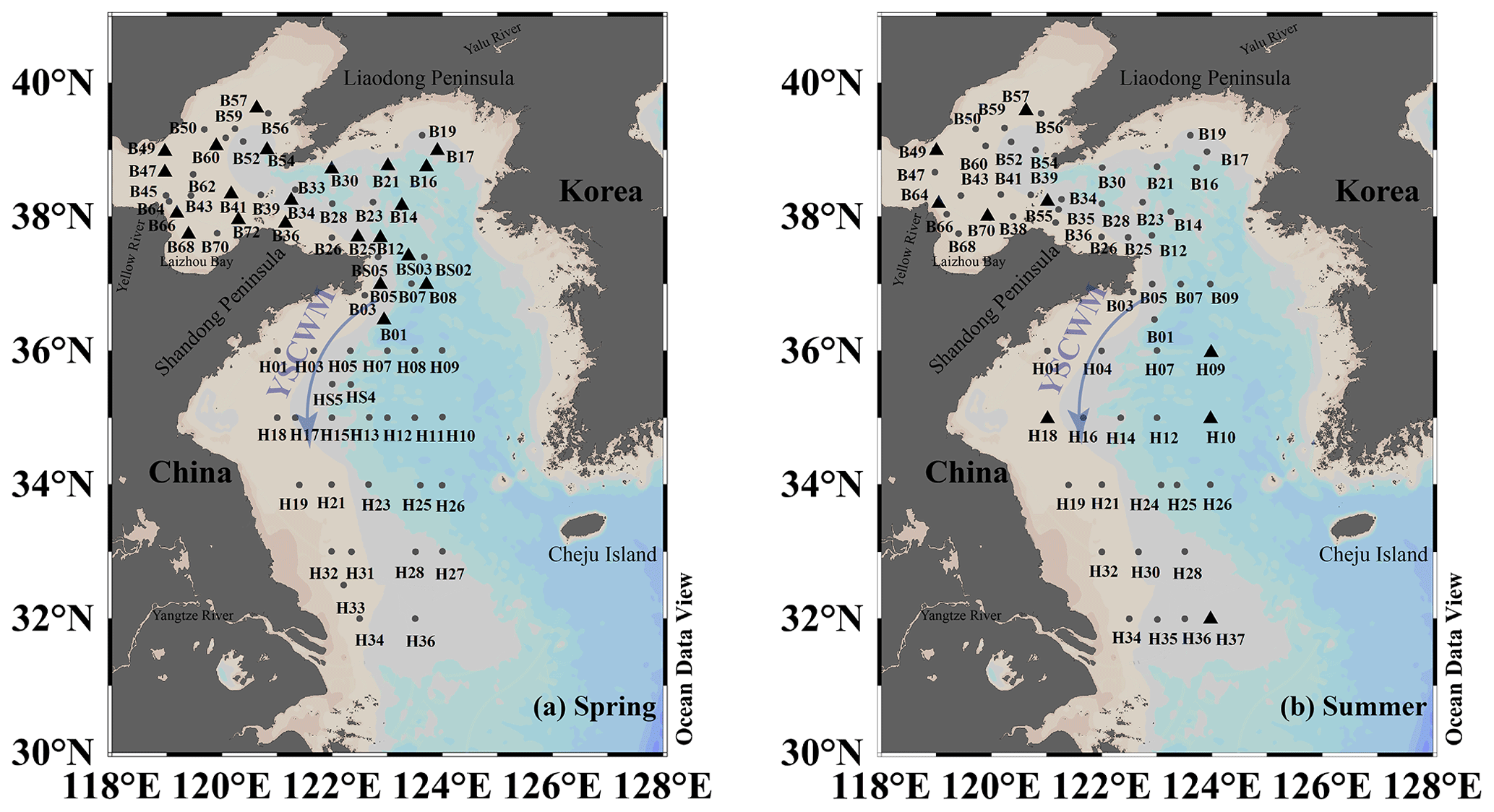
Figure 1Sampling stations in the Yellow Sea and Bohai Sea during (a) spring and (b) summer (▴ indicates stations where atmospheric samples were collected). YSCWM: Yellow Sea Cold Water Mass. The maps were plotted with Ocean Data View (ODV software) (Schlitzer, 2023).
2.2 Analytical procedures
The VSC concentrations in the seawater were measured using a gas chromatograph (GC) (Agilent 7890A, USA) with a flame photometric detector (FPD). The atmospheric VSC mixing ratios were measured using a GC equipped with a mass spectrometer (GC-MS) (Agilent 7890A/5975C, USA) using the methods of Inomata et al. (2006) and Staubes and Georgii (1993), respectively. A CP-Sil 5 CB column (30 m × 0.32 mm × 4.0 µm; Agilent Technologies, USA) was used to separate the three VSCs. Standard VSC gases with mixing ratios of 1 ppmv were obtained from Beijing Minnick Analytical Instrument Equipment Center. Qualitative analysis was conducted by comparing the results with the retention times of the standards, and quantitative analysis was conducted by diluting the VSC standard gases to 1 and 5 ppbv using a 2202A dynamic dilution meter (Nutech, USA) and injecting different volumes of the diluted VSC standards into the GC using a gas-tight syringe. The VSC mixing ratios were calculated after calibration using standard gases (Fig. S1 in the Supplement).
The VSC concentrations in seawater were determined using a cryogenic purge-and-trap system coupled with the GC-FPD. A 30 mL seawater sample was injected into a glass bubbling chamber with a gas-tight syringe (SGE, Australia). The VSCs were extracted from the seawater with high purity N2 at a rate of 60 mL min−1 for 15 min and passed through an anhydrous CaCl2-filled drying tube and a 100 % degreased cotton-filled 1/4 Teflon tube to remove water and oxides. Subsequently, the VSC gases were passed through a six-way valve and trapped in a loop of the 1/16 Teflon capture tube immersed in liquid nitrogen. After all VSCs had been purged from the seawater, the capture tube was removed from the liquid nitrogen and placed into hot water (> 90 ∘C) to desorb the trapped VSCs. The VSCs gases were carried into the GC by N2 and detected by the FPD. The column temperature was programmed with an initial temperature of 55 ∘C, followed by an increase to 100 ∘C at 10 ∘C min−1 and a final increase to 150 ∘C at 15 ∘C min−1. The inlet and detector temperatures were 150 and 160 ∘C, respectively, and the split ratio of pure N2 was 10:1. The detection limits of the method for COS, DMS, and CS2 were 33, 387, and 22 pg, and the measurement precision was 5.59 %–11.70 % (Tian et al., 2005). The DMS concentrations in seawater were obtained from Zhang et al. (2023).
The mixing ratios of atmospheric VSCs were analyzed using an Entech 7100 pre-concentrator (Nutech, USA) coupled with GC-MS. The sample SilcoCan canister was connected to the pre-concentrator, and 200 mL of gas was drawn into the preconcentration system with a three-stage cold trap (Fig. S1). The pre-concentrator parameters of the three-stage cold trap are listed in Table S1 in the Supplement. The first trap removes N2, O2, and H2O (g) from the atmospheric samples and the second trap eliminates CO2. The third trap is used to separate the three VSCs and obtain better peak shapes. The temperature programming of the column was the same as for the seawater samples. In addition, the temperature of the quadrupole and ion source were 110 and 230 ∘C, respectively, and the electron ionization source was run at 70 ev. The carrier gas had a split ratio of 10:1 and a flow rate of 2.0 mL min−1. Qualitative and quantitative analyses of the VSCs were conducted using the full scan mode (SCAN) and the selected ion monitoring mode (SIM). The mass-to-charge ratios (m/z) for COS, DMS, and CS2 were 60, 62, and 76, respectively. The detection limit of the VSCs was 0.1–0.5 pptv (Zhu et al., 2017).
2.3 Calculation of sea-to-air fluxes of VSCs
The sea-to-air fluxes of the VSCs were calculated using the model established by Liss and Slater (1974): F=kw (cw–cg/H), where F is the sea-to-air flux of VSCs (µmol m−2 d−1); kw is the VSC transfer velocity (m d−1); cw and cg are the equilibrium concentrations of VSCs in the surface seawater and the atmosphere (nmol L−1), respectively; and H is Henry's constant calculated using the equation listed in Table S2 (De Bruyn et al., 1995; Dacey et al., 1984). It was converted to a dimensionless constant using the equation proposed by Sander (2015). kw was calculated from the wind speed and the sea surface temperature was obtained by the N2000 method (Nightingale et al., 2000). The Cg of DMS is assumed to be zero in this study. This is based on the fact that atmospheric mixing ratios of DMS are typically several orders of magnitude lower than concentrations in seawater (Turner et al., 1996). We used the calculation developed by Kettle et al. (2001).
2.4 Measurements of Chl a, nutrients, and dissolved organic carbon
The seawater samples for the analysis of the Chl a concentrations were filtered through Whatman GF/F filters and the filtrate was stored in darkness at −20 ∘C. Then, Chl a was extracted with 90 % acetone for 24 h at 4 ∘C in darkness. The Chl a concentrations were determined following the method of Parsons et al. (1984) with a fluorescence spectrophotometer (F-4500; Hitachi, Japan) at excitation/emission wavelengths of 436 nm/670 nm. The seawater was filtered through Whatman GF/F filters (0.7 µm), and the filtered water samples were stored at −20 ∘C before nutrient (nitrate, phosphate, and silicate) analysis. A Technicon Autoanalyser AAII (SEAL Analytical, UK) was used to measure the nitrate, phosphate, and silicate concentrations. The nitrate, phosphate, and silicate data were provided by the open research cruise supported by the National Natural Science Foundation (NSFC) Shiptime Sharing Project.
The dissolved organic carbon (DOC) concentrations were measured using the method of Chen et al. (2021). The seawater was filtered through Whatman GF/F filters (pre-combusted at 500 ∘C for 4 h), and the filtrate was stored at −20 ∘C for DOC analysis. The DOC concentrations were determined by a total organic carbon analyzer (Shimadzu TOC-VCPH) after adding two drops of 12 mol L−1 HCl.
2.5 Data analysis
SPSS 24.0 software (SPSS Inc., USA) was used to analyze the relationships between the environmental factors and the concentrations and mixing ratios of the three VSCs in seawater and the atmosphere during spring and summer.
3.1 Spatial distributions of COS, DMS, and CS2 in surface seawater
3.1.1 Spring distributions
The temperature in the surface seawater showed a decreasing trend from south to north, and the salinity increased from the inshore to the offshore sites due to the influences of the YS warm current, Yalu River, and Yellow River (Fig. 2). The Chl a concentrations in the surface water of the BS and YS in the spring were 0.17–4.45 µg L−1 with an average of 1.19 ± 0.96 µg L−1. The highest Chl a concentration occurred at station B39 in the BS (Fig. 2), which may be related to the enhanced phytoplankton growth due to the abundance of nutrients resulting from a seawater exchange between the BS and YS. In addition, high Chl a concentrations were observed in the central area of the southern YS.
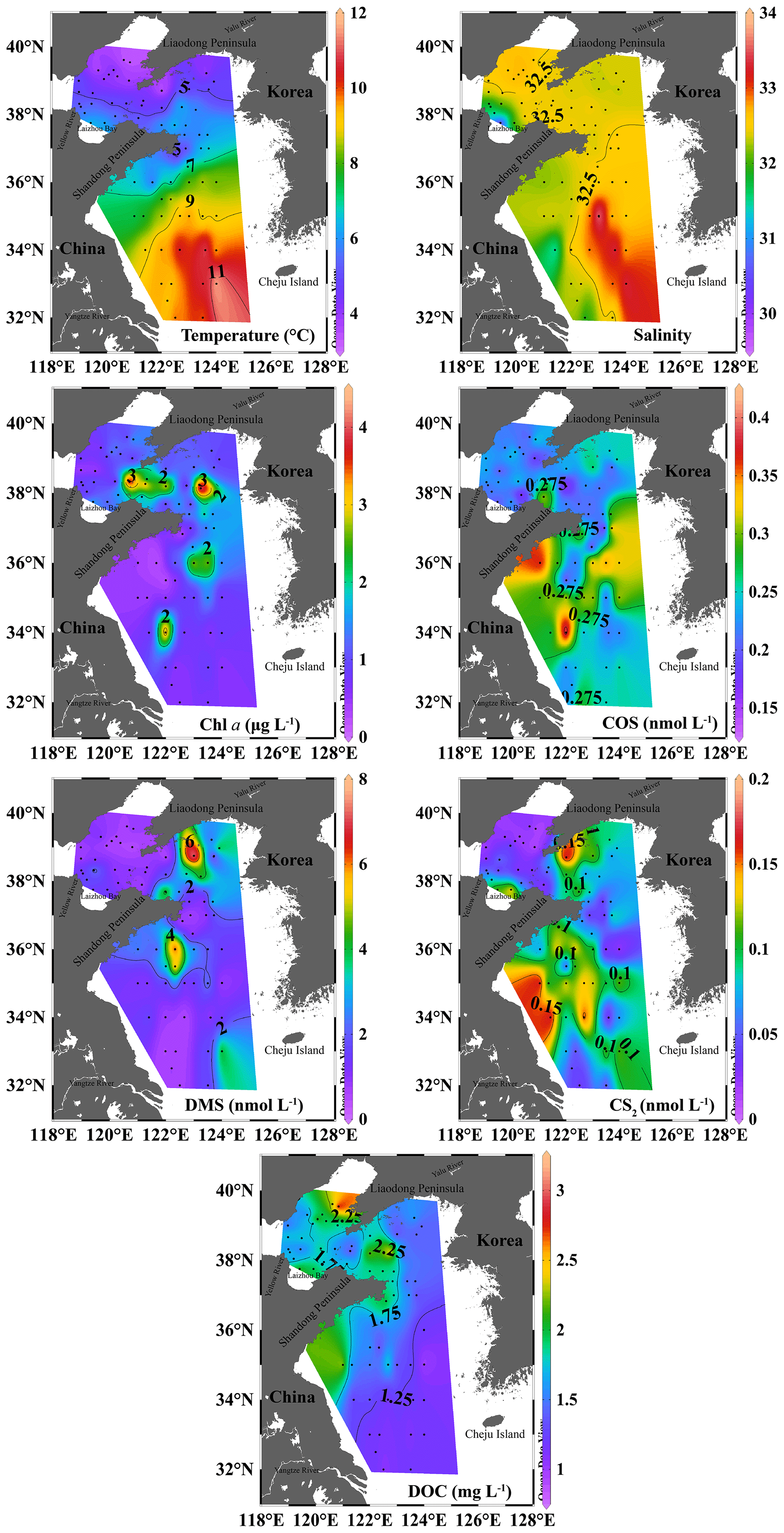
Figure 2Spatial distributions of temperature, salinity, Chl a, COS, DMS, CS2, and DOC in the surface water of the BS and YS in spring. The maps were plotted with Ocean Data View (ODV software) (Schlitzer, 2023).
The concentrations of COS, DMS, and CS2 in the surface seawater of the BS and YS during spring were 0.14–0.42, 0.41–7.74, and 0.01–0.18 nmol L−1, with mean values of 0.24 ± 0.06, 1.74 ± 1.61, and 0.07±0.05 nmol L−1, respectively (Fig. 2). The high COS concentrations during the spring occurred in the YS (Fig. 2). The highest COS concentration was observed at station H21, coinciding with a high Chl a concentration. The two areas with high concentrations of COS in the central waters of the southern YS overlapped with areas with high Chl a concentrations. High DMS concentrations existed in the coastal waters of the southern Shandong Peninsula, as well as at station B21 in the central part of the northern YS. The distribution of CS2 in seawater exhibited a decreasing trend from inshore to offshore (Fig. 2). High CS2 concentrations appeared at stations H18 and H19 in the coastal waters of YSCWM (Fig. 2). There was also a high CS2 concentration at station B30 near the shore of the Liaodong Peninsula (Fig. 2).
3.1.2 Summer distributions
The temperature and salinity in the BS and YS in summer were relatively high, and high Chl a concentrations were concentrated in coastal waters (Fig. 3). The Chl a concentrations in the seawater during summer were 0.10–4.74 µg L−1 with an average of 1.60 ± 1.19 µg L−1. Station B43 near the Yellow River estuary and Laizhou Bay had the highest Chl a concentration, which may have been due to the abundance of nutrients (nitrate: 5.85 µmol L−1; silicate: 17 µmol L−1) carried by nearby rivers or coastal currents (Figs. 3 and S2). Low salinities and high nitrate and Chl a concentrations occurred at Stations H32, H34, and H35 in the northeast of the Yangtze River estuary and at Stations B66 and B68 near the Laizhou Bay and Yellow River estuary (Figs. 3 and S2).
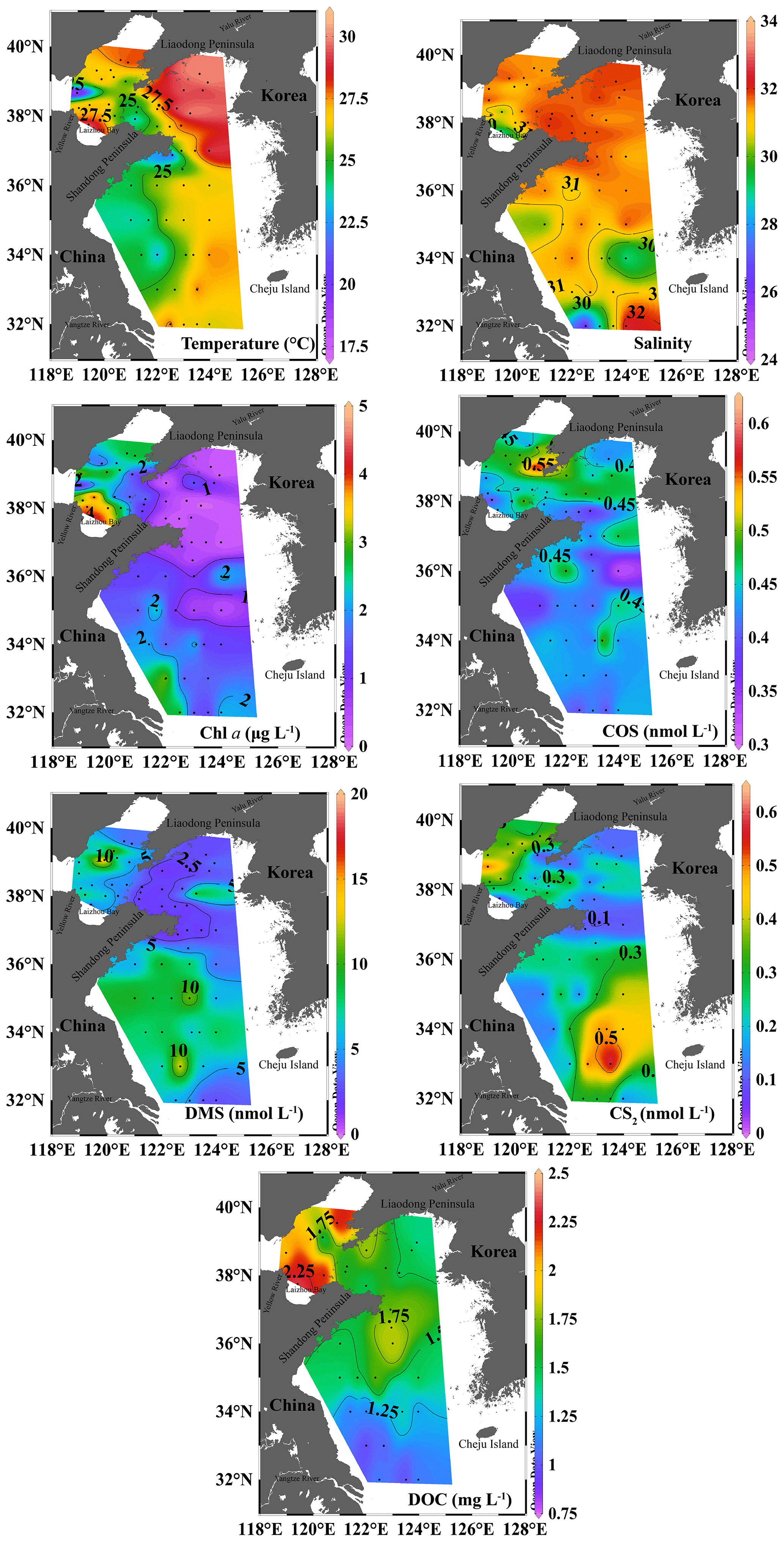
Figure 3Spatial distributions of temperature, salinity, Chl a, COS, DMS, CS2, and DOC in the surface water of the BS and YS in summer. The maps were plotted with Ocean Data View (ODV software) (Schlitzer, 2023).
The concentrations of COS, DMS, and CS2 in the surface water of the BS and YS during summer were 0.32–0.61, 1.31–18.12, and 0.01–0.65 nmol L−1, with mean values of 0.44 ± 0.06, 5.43 ± 3.60, and 0.26±0.15 nmol L−1, respectively (Fig. 3). The ratios of the mean concentrations between summer and spring for Chl a, COS, DMS, and CS2 were 1.3, 1.8, 3.1, and 3.7, respectively. High COS concentrations were observed at stations B38 and B54 in the BS during summer. In addition, COS had a high concentration at station H25 in the central part of the southern YS, close to a location with a high CS2 concentration (Fig. 3). High DMS concentrations were common in the northern BS and were generally coincident with high Chl a levels. However, high Chl a and DMS concentrations were found in the coastal waters of the Yangtze River estuary due to the Changjiang diluted water. In addition, the DMS concentration was high at station H12 (Fig. 3). There were high CS2 concentrations in the northeastern area of the Yangtze River estuary (Fig. 3).
3.2 Depth distributions of COS, DMS, and CS2 in seawater
3.2.1 Depth distributions in spring
The temperature and Chl a decreased from the surface to the bottom seawater (Fig. 4). The ratios of the mean concentrations between the surface and greater depths (> 60 m) were 5.4, 5.1, 5.9, and 8.9 for Chl a, COS, DMS, and CS2, respectively (Fig. 4). Consistent with the Chl a distribution, the depth distribution of DMS in the seawater decreased from the euphotic zone to the bottom seawater (Fig. 4). High COS concentrations occurred in the surface seawater and decreased with the depth, and the lowest concentrations occurred in the bottom waters. CS2 exhibited depth gradients at most stations during spring, with higher concentrations at the surface, except for station H15 where the CS2 concentrations were high in the bottom seawater.
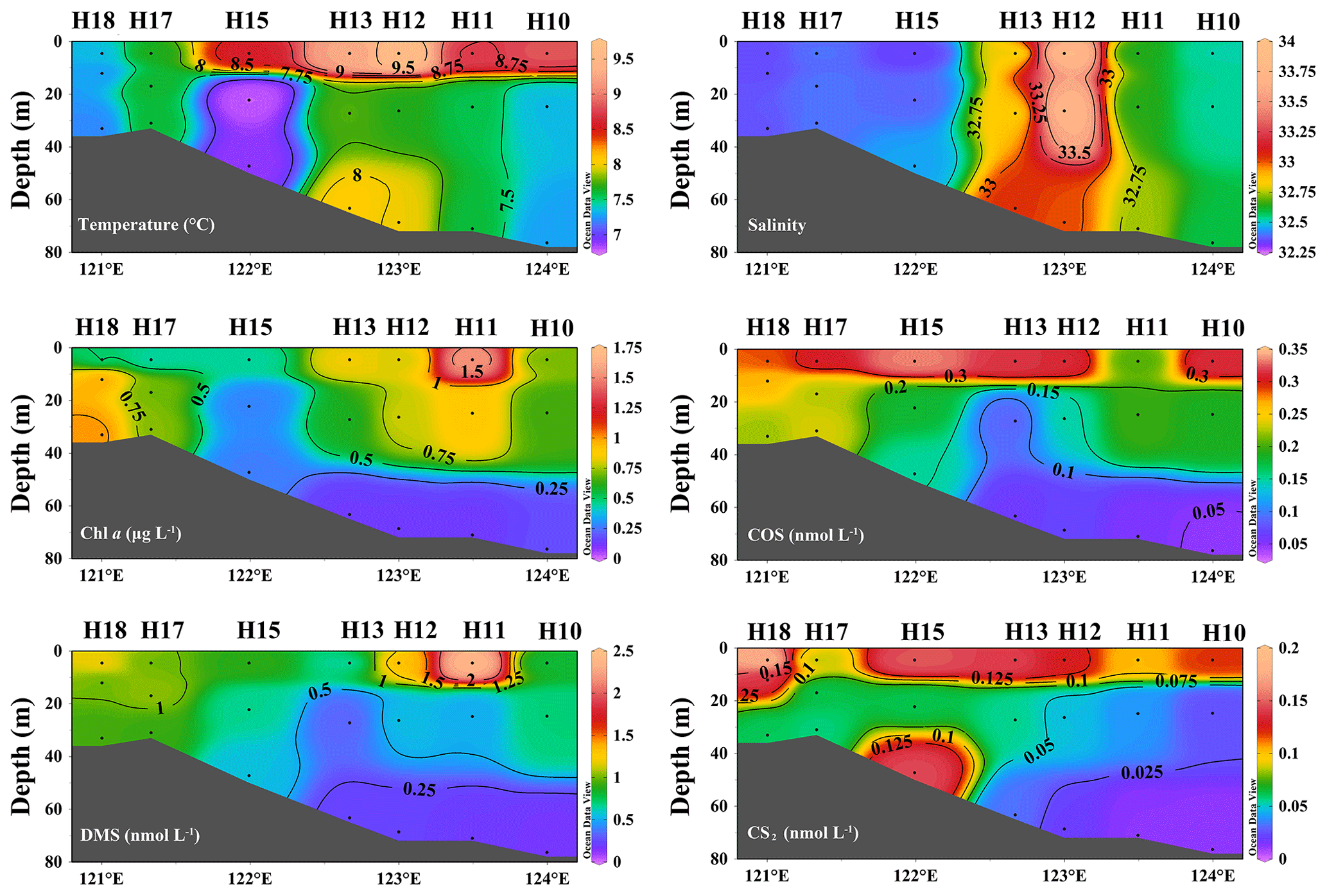
Figure 4Depth distributions of temperature, salinity, Chl a, COS, DMS, and CS2 in seawater in spring. The maps were plotted with Ocean Data View (ODV software) (Schlitzer, 2023).
3.2.2 Depth distributions in summer
The YSCWM affected the depth distributions in summer in the 35∘ N transect. Substantial temperature differences occurred between the surface and bottom seawater in summer, and stratification in the water bodies was observed (Fig. 5). A distinct thermocline existed at a depth of 20 m, indicating the formation of the YSCWM (Fig. 5). All high Chl a concentrations in the surveyed area of the BS and YS during summer occurred in the euphotic zone, and the highest concentrations occurred in waters at depths of 10–20 m (Fig. 5). The ratio of the mean Chl a concentration at depths of 10−20 m to depths > 60 m was 5.4. The depth distribution of DMS in seawater during summer decreased from the surface to the bottom seawater (Fig. 5). A significant depth gradient in the COS and CS2 concentrations occurred at most stations, exhibiting decreases with the increasing depth. The ratios of the mean concentrations of COS, DMS, and CS2 between the surface and depths > 60 m were 12.0, 8.6, and 11.5, respectively. However, the COS concentration was high in the bottom waters of station H16 (0.465 nmol L−1) (Fig. 5). The ratios of the mean concentrations of Chl a, COS, DMS, and CS2 of all samples at different depths between summer and spring were 2.2, 1.0, 5.6, and 2.0, respectively.
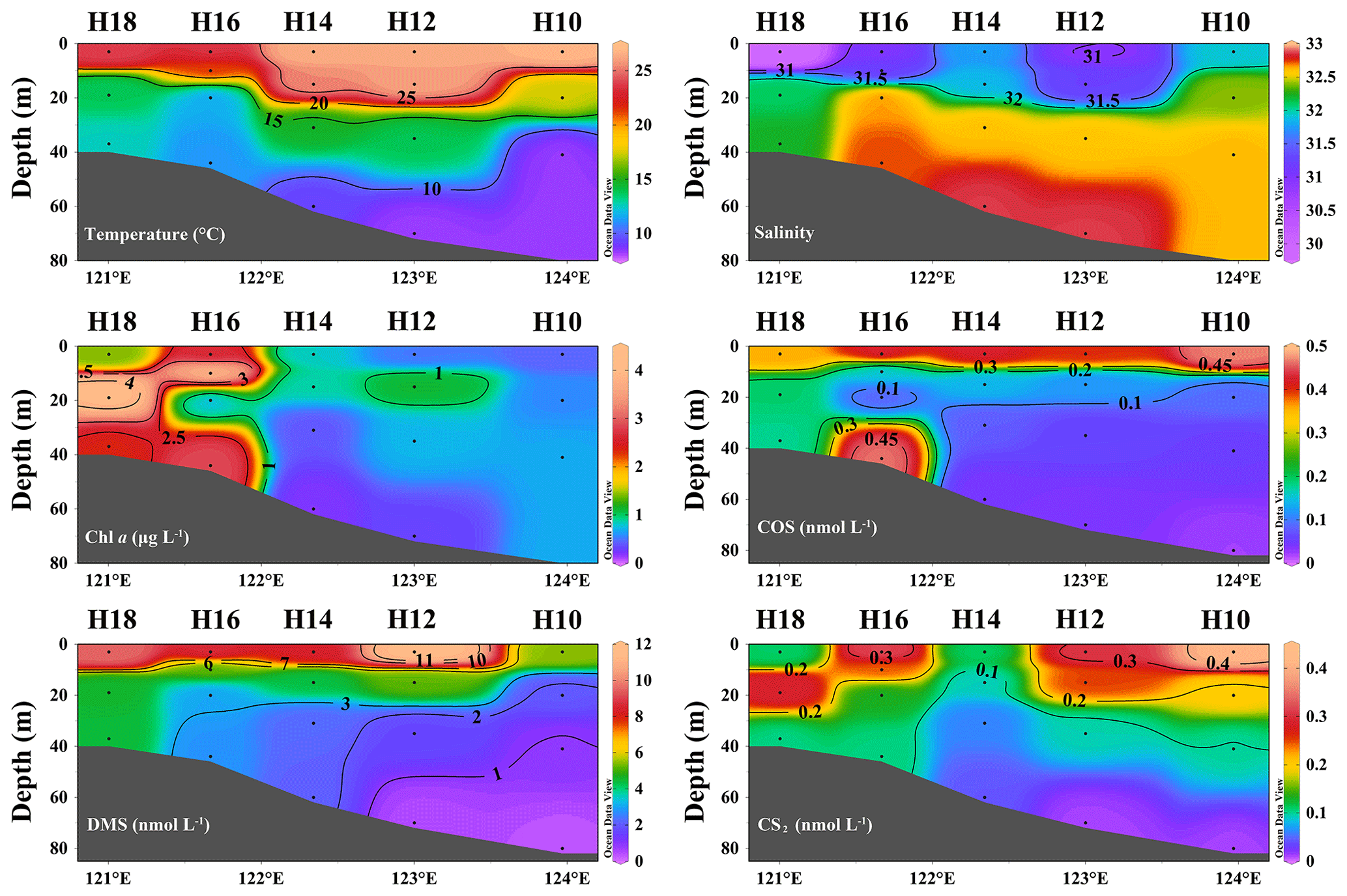
Figure 5Depth distributions of temperature, salinity, Chl a, COS, DMS, and CS2 in seawater in summer. The maps were plotted with Ocean Data View (ODV software) (Schlitzer, 2023).
3.3 VSCs in the atmosphere
3.3.1 Spring
The mixing ratios of COS, DMS, and CS2 in the atmosphere overlying the BS and YS in spring were in the ranges of 255.9–620.2, 1.3–191.2, and 5.2–698.8 pptv (Fig. 6a–c), and their mean mixing ratios were 345.6 ± 79.2, 47.5 ± 49.8, and 113.2 ± 172.3 pptv, respectively. The decreasing order of the mean mixing ratios of the three VSCs in the atmosphere during spring was COS > CS2 > DMS. The highest mixing ratio of atmospheric COS occurred at station B72 (Fig. 6a) near the northern Shandong Peninsula. The highest atmospheric DMS mixing ratio was observed at station B08 (Fig. 6b). The DMS concentration in the seawater (Fig. 2) was not as high as that in the atmosphere at station B49 (Fig. 6b). According to the 72 h backward trajectory map (Fig. S3), the air mass over station B49 had migrated from the land to the ocean, passing through Beijing, Tianjin, and other densely populated areas. The air mass over station B47 differed slightly from that over station B49 as it traversed the land of Liaoning province (12 h and 24 h backward trajectories in Fig. S3). The lowest atmospheric DMS mixing ratio was observed at station B47 (Fig. 6b), probably due to the low DMS concentration in seawater (0.5 nmol L−1) and the loss across the land. The highest atmospheric DMS mixing ratio occurred at station B08 (Fig. 6b). In addition, there were high mixing ratios of CS2 at stations in the BS, such as B57, B60, and B72, and low mixing ratios at stations B17 and B21 in the northern YS (Fig. 6c).
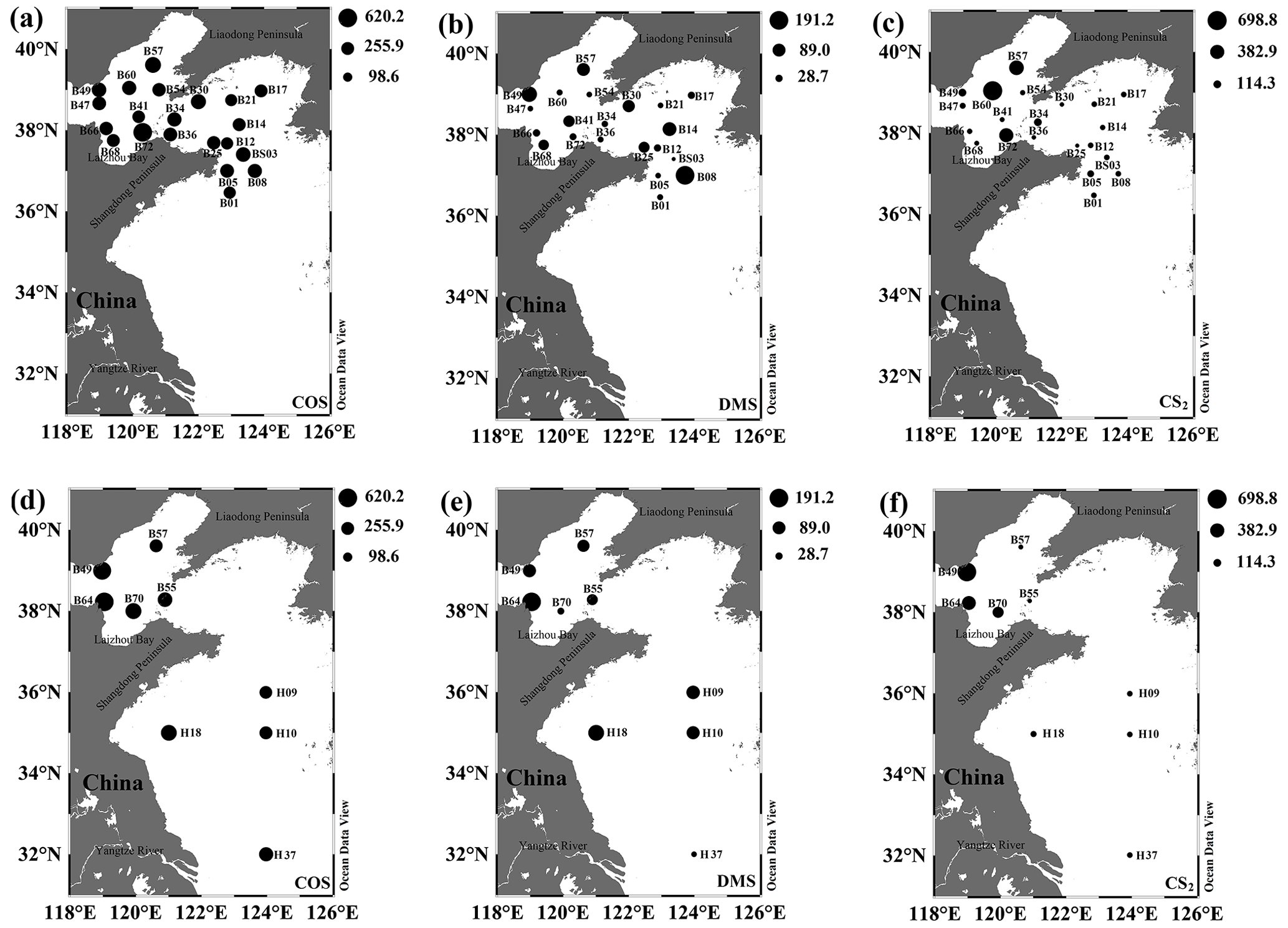
Figure 6Spatial distributions of COS, DMS, and CS2 in the atmosphere over the BS and YS in (a)–(c) spring and (d)–(f) summer (unit: pptv). The maps were plotted with Ocean Data View (ODV software) (Schlitzer, 2023).
3.3.2 Summer
The mixing ratios of COS, DMS, and CS2 in summer ranged from 394.6 to 850.1 pptv, from 10.3 to 464.3 pptv, and from 15.3 to 672.7 pptv, with mean values of 563.8 ± 168.9, 216.6 ± 136.0, and 164.4±225.5 pptv, respectively (Figs. 6d–f). The order of the three VSCs in terms of the mean mixing ratios in the atmosphere during summer was COS > DMS > CS2. The ratios of the mean mixing ratios for atmospheric COS, DMS, and CS2 between summer and spring were 1.6, 4.6, and 1.5, respectively. The three VSCs in the atmosphere over the BS and YS had similar spatial distributions. COS and DMS exhibited the highest mixing ratios at station B64 (Fig. 6d and e). The highest mixing ratio of CS2 in summer appeared at station B49 near the shore and the lowest one occurred far from shore at station H09 (Fig. 6f). The air masses over stations B49, B64, and H09 had migrated from the land, land, and ocean, respectively (Fig. S3). The distributions of CS2 showed a decreasing trend from inshore to offshore (Fig. 6f).
3.4 Relationships between environmental factors and COS, DMS, and CS2 concentrations
A significant correlation was found between the DMS and CS2 concentrations in the surface seawater in spring (P<0.05) and summer (P<0.01) (Table 1). A positive correlation occurred between the COS and DOC concentrations in seawater (P<0.05) and between the CS2 and Chl a concentrations in seawater (P<0.05) during summer (Table 1). There was a significant correlation between the atmospheric COS and CS2 mixing ratios in spring and summer (P<0.01) (Table 1).
Table 1Correlation analyses of the three VSCs and environmental factors in the BS and YS in spring and summer.
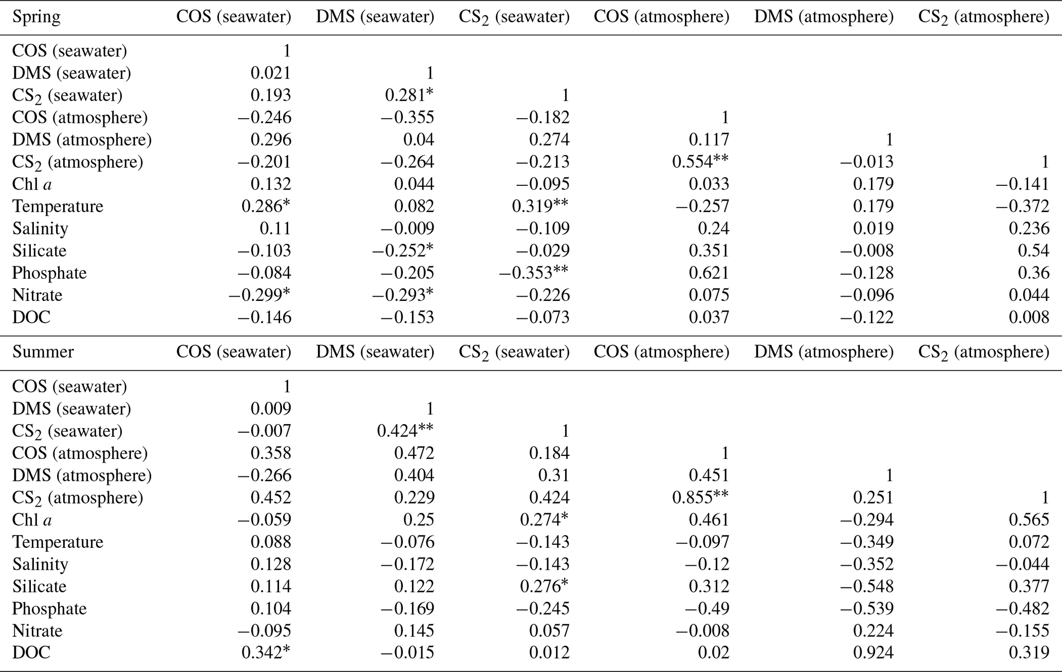
∗ Indicates P<0.05. Indicates P<0.01.
3.5 Sea-to-air fluxes of VSCs
3.5.1 Spring
The sea-to-air fluxes of COS, DMS, and CS2 in spring were 0.03–1.59, 0.06–25.40, and 0.003–0.30 µmol m−2 d−1, with averages of 0.50 ± 0.38, 2.99 ± 4.24, and 0.09 ± 0.08 µmol m−2 d−1, respectively (Fig. 7). The highest COS sea-to-air flux was observed at station B36, which had a high wind speed (11.3 m s−1). In comparison, the lowest COS sea-to-air flux occurred at station B12, where the minimum wind speed occurred (1.5 m s−1). The lowest sea-to-air fluxes of DMS and CS2 occurred at stations H01 and B41 (Fig. 7), where the wind speeds were 0.4 and 2 m s−1, respectively. The highest DMS and CS2 sea-to-air fluxes appeared at stations HS4 and B68, respectively, due to high wind speeds and high DMS and CS2 concentrations in seawater (Fig. 7).
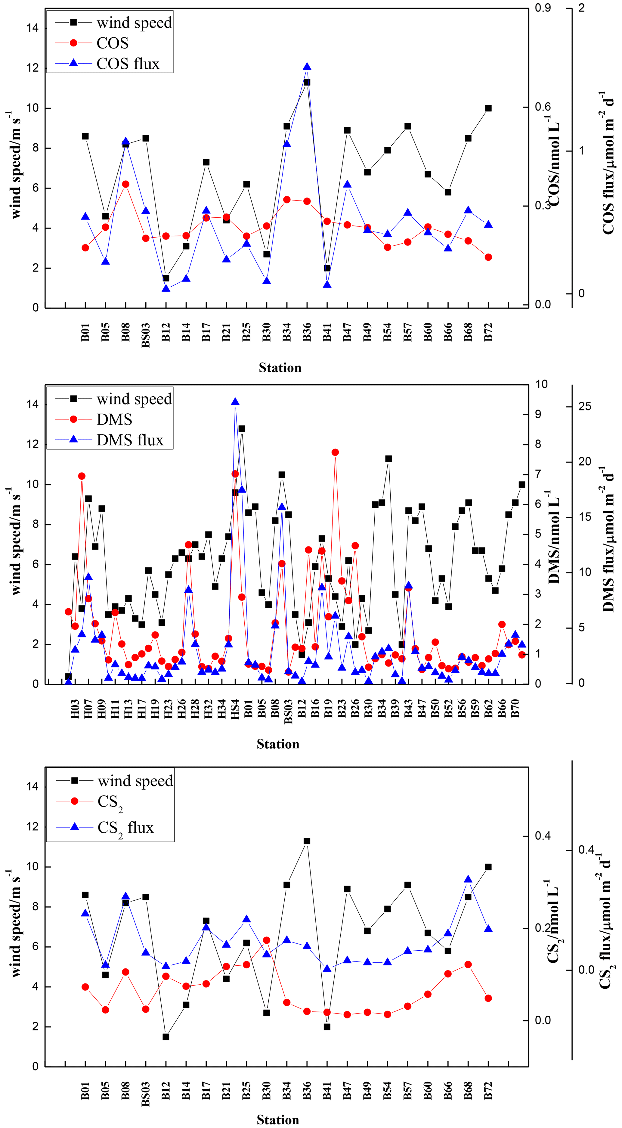
Figure 7Variations in sea-to-air fluxes of VSCs, VSC concentrations in seawater, and wind speeds in the BS and YS in spring 2018.
3.5.2 Summer
The sea-to-air fluxes of COS, DMS, and CS2 in summer were 0.06–1.51, 0.10–25.44, and 0.02–0.99 µmol m−2 d−1, with averages of 0.60 ± 0.59, 6.26 ± 6.27, and 0.39 ± 0.42 µmol m−2 d−1, respectively (Fig. 8). The ratios of the mean sea-to-air fluxes for COS, DMS, and CS2 between summer and spring were 1.2, 2.1, and 4.3, respectively. Consistent with their order in seawater, the order of the sea-to-air fluxes of the VSCs was DMS > COS > CS2. The lowest sea-to-air fluxes of COS, DMS, and CS2 in summer occurred at stations B64, B05, and B57, which had the low wind speeds of 1, 0.4, and 1.1 m s−1, respectively, and low seawater VSC concentrations. The highest sea-to-air flux of COS and DMS occurred at stations B70 and H14, respectively, coinciding with high wind speeds and high COS and DMS concentrations in seawater (Fig. 8). The maximum CS2 sea-to-air flux appeared at station H09, where the concentration of CS2 in seawater was 0.31 nmol L−1 (Fig. 8).
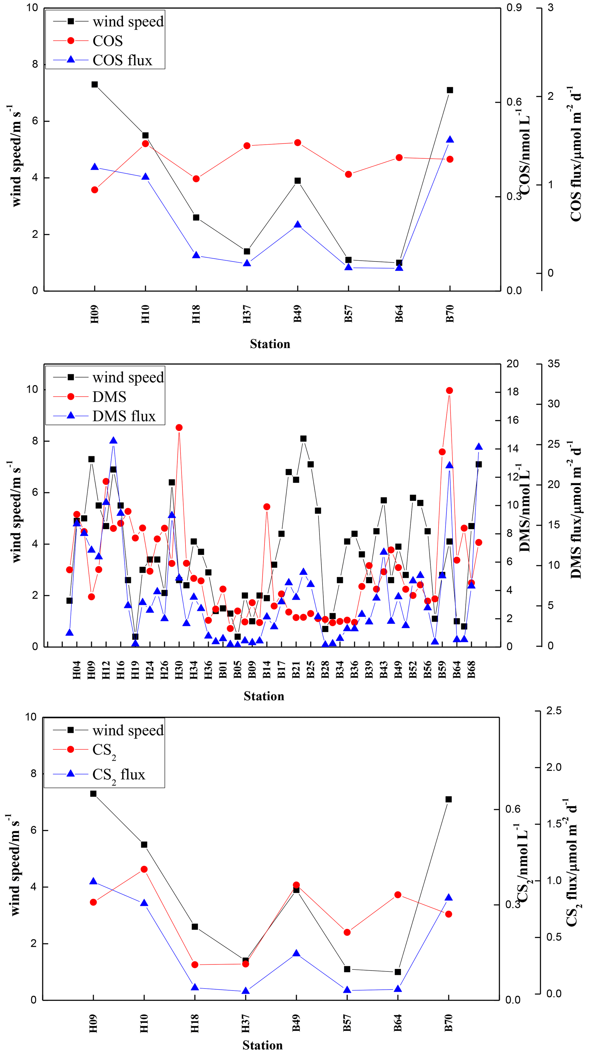
Figure 8Variations in sea-to-air fluxes of VSCs, VSC concentrations in seawater, and wind speeds in the BS and YS in summer 2018.
4.1 Spatial and depth distributions and seasonal variations in VSCs in seawater
4.1.1 Spatial distributions of VSCs and the impact factors
The COS concentrations in this study were similar to those in six tidal European estuaries (Scheldt, Gironde, Rhine, Elbe, Ems, and Loire) (0.22 nmol L−1) (Sciare et al., 2002), the DMS concentrations were lower than previous observations in the BS and YS in autumn (3.92 nmol L−1) (Yang et al., 2014), and the CS2 concentrations were lower than those in the coastal waters off the eastern coast of the United States (0.004–0.51 nmol L−1) (Kim and Andreae, 1992). Furthermore, the VSC concentrations in the seawater of the BS and YS were significantly higher than those in oceanic areas, such as the North Atlantic Ocean (Simó et al., 1997; Ulshöfer et al., 1995). The higher CDOM concentrations in the nearshore waters may be the reason for the difference (Guéguen et al., 2005). Zepp and Andreae (1994) demonstrated that the photosensitized reaction of organosulfur compounds contributed to the production of COS. The reaction rates in coastal waters may be higher than those in open sea. Our results showed that the average COS, DMS, and CS2 concentrations in the surface seawater of the BS and YS during summer were higher than those in the Changjiang estuary and the adjacent East China Sea (Yu et al., 2022). The reasons may be different sea areas, temperatures, and industrial production. The mean concentrations of COS, DMS, and CS2 in the surface seawater of the BS and YS during both spring and summer were 0.34, 3.41, and 0.16 nmol L−1, respectively. The mean COS and CS2 concentrations were approximately one order of magnitude higher than the global values reported by Lennartz et al. (2020), which were 32.3 and 15.7 pmol L−1. Lennartz et al. (2020) highlighted that the COS concentrations in estuaries and shelves were 10- to 1000-fold higher than those in oligotrophic waters. This disparity in concentrations may account for the discrepancies observed between our findings and global values. In comparison, the mean DMS concentration was similar to the value reported by Hulswar et al. (2022), which was 2.26 nmol L−1.
Different production and consumption mechanisms resulted in different spatial distributions of COS, DMS, and CS2. DMS and DMSP concentrations are related to the composition and abundance of phytoplankton (Kurian et al., 2020; Naik et al., 2020; O'Brien et al., 2022; Yu et al., 2023a). The highest DMS concentrations at station B21 in spring coincided with high Chl a concentrations (Fig. 2). Low salinities (< 30) occurred at stations H25, H26, H34, H35, B43, B66, and B68 due to river water discharge from the Yangtze River estuary, Yellow River, and Laizhou Bay in summer, consistent with the high nitrate, silicate, Chl a, and DMS concentrations (Figs. 3 and S2). High CS2 concentrations in the coastal waters of the Yellow River estuary and at stations H18, H19, and B30 in spring may be due to high CDOM carried by the YS coastal current and Yellow River and terrestrial input. The significant correlation between the DMS and CS2 concentrations in the surface seawater was consistent with the results of Ferek and Andreae (1983) and Yu et al. (2022). DMS in seawater is primarily derived from the degradation of DMSP, which is released from algal cell lysis (O'Brien et al., 2022). Moreover, the algae decay increased the CS2 emission rate due to the degradation of sulfur-containing amino acids (Wang et al., 2023). The commonality of their sources resulted in a high correlation between the DMS and CS2 concentrations in seawater. Xie et al. (1998) pointed out that CS2 has a photochemical production mechanism similar to that of COS. Both are primarily produced by photochemical reactions of thiol-containing compounds, such as methyl mercaptan (MeSH) or glutathione, under the catalysis of CDOM. Terrestrial CDOM has higher photochemical reactivity and is more conducive to the photochemical generation of CS2 (Xie et al., 1998). COS production rates increase with an increase in the absorption coefficient at 350 nm (a350) (Li et al., 2022). Uher and Andreae (1997) showed that the COS concentration in seawater was significantly correlated with the CDOM concentration. The positive correlation between the COS and DOC concentrations in seawater during summer in this study suggested that COS was produced by the photochemical reaction of CDOM. COS and CS2 are formed via a reaction between cysteine and intermediates (i.e., CDOM• and •OH) (Chu et al., 2016; Du et al., 2017; Modiri Gharehveran et al., 2020). Modiri Gharehveran and Shah (2021) showed that DOM could photochemically produce 3CDOM∗, 1O2, H2O2, and •OH by sunlight reacting with DMS, forming a sulfur- or carbon-centered radical and subsequently COS and CS2. Li et al. (2022) demonstrated that a high nitrate concentration resulted in a high COS production rate. The high COS concentrations at stations H25 and B43 during summer coincided with high nitrate concentrations (Figs. 3 and S2). However, no significant correlations were found between the COS and nitrate concentrations during summer (Table 1).
4.1.2 Depth distributions of VSCs and impact factors
The depth distributions of DMS, COS, and CS2 showed similar patterns: their concentrations decreased with increasing depth, in agreement with the results of Yu et al. (2022). Yu et al. (2023a) also showed that the DMS concentrations in the 35∘ N transect of the BS and YS in autumn decreased with an increase in seawater depth. The highest Chl a concentrations during summer occurred at depths of 10–20 m. This result was attributed to the abundance of nutrients and suitable water temperatures near the thermocline, benefitting phytoplankton growth. Yu et al. (2021) reported that the highest DMSP-consuming bacterial abundance and DMSP lyase activity at the 35∘ N transect in the summer of 2013 occurred at depths of 10–15 m, consistent with our Chl a concentrations. DMS originates primarily from phytoplankton; thus, its concentration trend is similar to that of Chl a. COS and CS2 in seawater are predominantly derived from photochemical reactions of organic sulfides catalyzed by CDOM; therefore, light is the limiting factor for their production in seawater (Uher and Andreae, 1997). Ulshöfer et al. (1996) studied the depth distribution of COS in seawater and found that high COS concentrations occurred in the euphotic zone. The high COS concentrations in the surface seawater in this study may be attributed to the photochemical production reactions of CS2 and COS in the euphotic zone because they are dependent on light (Flöck et al., 1997; Xie et al., 1998). The addition of photosensitizers-natural DOM and commercial humic acid (HA) photo-catalyzed glutathione (GSH) and cysteine, and enhanced the COS formation (Flöck et al., 1997). An excited triplet state CDOM (3CDOM∗) is produced by COS in the presence of ultraviolet light (Li et al., 2022). In addition, the loss processes include exhalation, downward mixing, and hydrolysis, with hydrolysis being identified as the predominant sink (Xu et al., 2001). We speculate that a slow hydrolysis rate may be another reason accounting for the high COS concentrations in the surface seawater. Hobe et al. (2001) stated that the non-photochemical production of COS is critical for the global budget. Consistent with Hobe et al. (2001), the high COS concentration in the bottom waters at station H16 in summer may be related to the non-photochemical production of COS or release by underlying sediments. Consistent with our CS2 results, Xie et al. (1998) showed that the CS2 concentrations decreased with the depth, coinciding with solar radiation changes. Decreased photochemical reaction due to decreasing solar radiation with water depth may explain the vertical distribution of CS2 (Xie et al., 1998). Similar to the results of Xie et al. (1998), the high CS2 concentrations in the bottom seawater at station H15 in spring may be attributable to a sedimentary source.
4.1.3 Seasonal and diurnal variations in VSCs in seawater
The VSCs in seawater exhibited significant seasonal differences (VSCs in summer > VSCs in spring) in this study. Similar seasonal variations in COS were also observed by Xu et al. (2001), who found that the COS concentrations in South Africa were higher in summer than in autumn. In addition, observations by Weiss et al. (1995) showed that the COS concentrations in the seawater of the Atlantic and Pacific oceans were very low in winter. Xu et al. (2001) concluded that warmer seasons and high biological productivity resulted in enhanced COS concentrations. The significant correlation between the oceanic COS concentrations and the temperatures in spring (Table 1) can prove this. Xie et al. (1998) showed that the order of the CS2 production rates was summer > spring > fall > winter. The significant positive correlations between the CS2 and Chl a concentrations during summer may explain the higher CS2 concentration in seawater during summer than during spring in this study. Similar to the seasonal changes in Chl a, the DMS concentrations were higher in summer than in spring. A higher phytoplankton biomass in summer has been linked to higher DMS concentrations in summer than in autumn (Yang et al., 2015). In addition, diurnal variations in the COS concentrations in seawater (high during the day and low at night) were reported (Ferek and Andreae, 1984; Lennartz et al., 2017; Xu et al., 2001). COS photoproduction via photochemical reactions is more rapid than hydrolysis during the day (Xu et al., 2001). Furthermore, the COS concentration depends on the light intensity (Ferek and Andreae, 1984). Therefore, the sampling time can influence the measured COS concentrations in the seawater.
4.2 VSCs in the atmosphere
The mean mixing ratios of COS and CS2 in the atmosphere overlying the BS and YS during both spring and summer were 411.0 and 128.6 pptv, respectively. These values were 0.75-fold and 3.05-fold of the global scale values reported by Lennartz et al. (2020), which were 548.9 and 42.2 pptv. Similar to our results for the VSC mixing ratios in the atmosphere during summer, Kettle et al. (2001) found that the COS mixing ratio in the Atlantic Ocean atmosphere was 552 pptv, while Cooper and Saltzman (1993) measured a DMS mixing ratio of 118 pptv. In addition, the mixing ratios of atmospheric CS2 in this study were similar to those in a polluted atmosphere (Sandalls and Penkett, 1977) but much higher than those in unpolluted atmospheres, such as over the North Atlantic (Cooper and Saltzman, 1993). This finding indicated that industrial production and human activities significantly affect the mixing ratios of CS2 in the atmosphere. The mean VSC mixing ratios in the atmosphere during summer in this study were all higher than those in the Changjiang estuary and the adjacent East China Sea (Yu et al., 2022), and the western Pacific during autumn (Xu et al., 2023).
No significant correlation was found between the oceanic VSC concentrations and atmospheric VSC mixing ratios (Table 1). The reason may be that VSCs in the atmosphere were not only derived from sea-to-air diffusion but also from anthropogenic sources, such as the soil, incomplete burning of biomass, and industrial releases (Blake et al., 2004; Chin and Davis, 1993; Whelan et al., 2018). Anthropogenic VSC emissions can be evaluated using isotope measurements (Hattori et al., 2020). However, anthropogenic VSC emissions were not evaluated in this study, and isotope measurements will be obtained in future studies. The highest mixing ratios of atmospheric COS at station B72 and DMS at station B08 in spring coincided with anthropogenic emissions and high DMS concentration in seawater, respectively (Fig. 6). The CS2 generated by industrial activities may have influenced the atmosphere at station B49, which is near industrial cities such as Tianjin. Chemical production and pharmaceutical industries are large emitters of CS2 into the atmosphere (Chin and Davis, 1993). CS2 is the main precursor of COS in the atmosphere, and atmospheric CS2 is oxidized to COS by radicals such as OH with a conversion efficiency of 0.81 (Chin and Davis, 1995). The significant correlation between atmospheric COS and CS2 in our study (Table 1) demonstrated this.
The tropospheric lifetimes of COS, CS2, and DMS were found to be 2–7 years, several days, and approximately 24 h, respectively (Lennartz et al., 2020; Khan et al., 2016). Backward trajectories in 12, 24, and 72 h were used to identify the sources of these compounds in our study (Fig. S3). The 72 h backward trajectories showed that air masses from different sources (land or ocean) and passing through different regions may have affected the atmospheric COS, DMS, and CS2 mixing ratios. Jiang et al. (2021) stated that different sources of air masses might have affected atmospheric DMS oxidation to MSA. The 72 h backward trajectory over station B49 indicated that the high atmospheric DMS mixing ratio was attributable to human activities. The wind direction is from continental Asia to the Pacific in spring. The backward trajectories of B49, B47, and B08 showed that anthropogenic and oceanic DMS emissions accounted for the atmospheric DMS sources. The wind direction of the air mass from the backward trajectories of Miyakojima, Yokohama, and Otaru in Japan in winter (January to March) observed by Hattori et al. (2020) was similar to ours in spring (March to April). Hattori et al. (2020) reported that the anthropogenic COS originated primarily from the Chinese industry and was transported by air to southern Japan. The backward trajectory of H09 showed that the wind direction was from the south of Taiwan Island in summer, and oceanic sources accounted for the atmospheric DMS. The air masses showed that the highest mixing ratios of COS and DMS at station B64 in summer were caused by terrestrial sources from northeast China and oceanic sources in the BS, respectively. The highest CS2 mixing ratio in summer at station B49 may be due to the air mass transported from the northeast, i.e., industrial cities in China.
4.3 Sea-to-air fluxes of VSCs
The mean sea-to-air fluxes of DMS in spring (2.99 µmol S m−2 d−1) and summer (6.26 µmol S m−2 d−1) observed in our study fell within the range of global DMS fluxes, which ranged from 0 to 10 µmol S m−2 d−1 (Hulswar et al., 2022). The calculated DMS sea-to-air fluxes in our study should be seen as upper limits due to setting the atmospheric mixing ratio to zero. The spatial variability in the sea-to-air fluxes was consistent with changes in the wind speed because sea-to-air fluxes depend on the transmission velocities of VSCs in seawater, which are related to the wind speed and viscosity of seawater. In addition, the sea-to-air fluxes of all three VSCs were positive in spring and summer, indicating that the seawater was a source of COS, DMS, and CS2 to the atmosphere through sea-to-air diffusion. Although our findings agree with those of Chin and Davis (1993) and Yu et al. (2022), who showed that the ocean was a major atmospheric source of COS, they conflict with the results of Weiss et al. (1995) and Zhu et al. (2019), who found significant COS undersaturation in some sea areas. Therefore, the ocean may be a sink of atmospheric COS in some areas or at certain times of the year.
The COS, DMS, and CS2 distributions in the surface seawater and marine atmosphere of the BS and YS during spring and summer exhibited significant spatial and seasonal variability. First, the COS, DMS, and CS2 concentrations were higher in summer than in spring. Second, the COS, DMS, and CS2 concentrations were the highest in the surface seawater and decreased with the depth. The positive correlation between the oceanic COS and DOC concentrations in summer suggested the photochemical production of COS from CDOM. In addition, the atmospheric VSC mixing ratios of the BS and YS exhibited substantial seasonal differences, with higher mixing ratios in summer than in spring. There was a significant correlation between the atmospheric COS and CS2 mixing ratios, which may verify the COS production from oxidation of CS2. The backward trajectories showed that the atmospheric mixing ratios of VSCs were affected by anthropogenic and/or oceanic emissions. Finally, the high sea-to-air fluxes of COS, DMS, and CS2 in the BS and YS indicated that marginal seas are important sources of atmospheric VSCs and may contribute considerably to the global sulfur budget.
Data to support this article are available at https://doi.org/10.6084/m9.figshare.14971644 (Yu et al., 2023b).
The supplement related to this article is available online at: https://doi.org/10.5194/bg-21-161-2024-supplement.
All authors were involved in the writing of the paper and approved the final version. YJ and YL were major contributors to the study's conception and data analysis, and writing of the manuscript. HZ, LJG, and LQ contributed significantly to writing the original draft. YGP contributed to reviewing and editing the manuscript.
The contact author has declared that none of the authors has any competing interests.
Publisher’s note: Copernicus Publications remains neutral with regard to jurisdictional claims made in the text, published maps, institutional affiliations, or any other geographical representation in this paper. While Copernicus Publications makes every effort to include appropriate place names, the final responsibility lies with the authors.
We are grateful to the captain and crew of the R/V Dong Fang Hong 2 for their help and cooperation during the in situ investigation.
This work was funded by the National Natural Science Foundation of China (grant nos. 41976038 and 41876122) and the National Key Research and Development Program (grant no. 2016YFA0601301).
This paper was edited by Hermann Bange and reviewed by two anonymous referees.
Andreae, M. O. and Crutzen, P. J.: Atmospheric aerosols: biogeochemical sources and role in atmospheric chemistry, Science, 276, 1052–1058, https://doi.org/10.1126/science.276.5315.1052, 1997.
Aydin, M., Britten, G. L., Montzka, S. A., Buizert, C., Primeau, F. W., Petrenko, V. V., Battle, M. O., Nicewonger, M. R., Patterson, J., Hmiel, B., and Saltzman, E. S.: Anthropogenic impacts on atmospheric carbonyl sulfide since the 19th century inferred from polar firn air and ice core measurements, J. Geophys. Res.-Atmos., 125, e2020JD033074, https://doi.org/10.1002/essoar.10503126.1, 2020.
Blake, N. J., Streets, D. G., Woo, J.-H., Simpson, I. J., Green, J., Meinardi, S., Kita, K., Atlas, E., Fuelberg, H. E., Sachse, G., Avery, M. A., Vay, S. A., Talbot, R. W., Dibb, J. E., Bandy, A. R., Thornton, D. C., Rowland, F. S., and Blake, D. R.: Carbonyl sulfide and carbon disulfide: large-scale distributions over the western Pacific and emissions from Asia during TRACE-P, J. Geophys. Res.-Atmos., 109, D15S05, https://doi.org/10.1029/2003JD004259, 2004.
Brown, A. S., van der Veen, A. M. H., Arrhenius, K., Murugan, A., Culleton, L. P., Ziel, P. R., and Li, J.: Sampling of gaseous sulfur-containing compounds at low concentrations with a review of best-practice methods for biogas and natural gas applications, Trac-Trends Anal. Chem., 64, 42–52, https://doi.org/10.1016/j.trac.2014.08.012, 2015.
Brühl, C., Lelieveld, J., Crutzen, P. J., and Tost, H.: The role of carbonyl sulphide as a source of stratospheric sulphate aerosol and its impact on climate, Atmos. Chem. Phys., 12, 1239–1253, https://doi.org/10.5194/acp-12-1239-2012, 2012.
Campbell, J. E., Carmichael, G. R., Chai T., Mena-Carrasco, M., Tang, Y., Blake, D. R., Blake, N. J., Vay, S. A., Collatz, G. J., Baker, I., Berry, J. A., Montzka, S. A., Sweeney, C., Schnoor, J. L., and Stanier, C. O.: Photosynthetic control of atmospheric carbonyl sulfide during the growing season, Science, 322, 1085–1088, https://doi.org/10.1126/science.1164015, 2008.
Campbell, J. E., Whelan, M. E., Seibt U., Smith S. J., Berry, J. A., and Hilton, T. W.: Atmospheric carbonyl sulfide sources from anthropogenic activity: Implications for carbon cycle constraints, Geophys. Res. Lett., 42, 3004–3010, https://doi.org/10.1002/2015GL063445, 2015.
Charlson, R. J., Lovelock, J. E., Andreae, M. O., and Warren, S. G.: Oceanic phytoplankton, atmospheric sulphur, cloud albedo and climate, Nature, 326, 655–661, https://doi.org/10.1038/326655a0, 1987.
Chen C.-T. A.: Chemical and physical fronts in the Bohai, Yellow and East China seas, J. Mar. Syst., 78, 394–410, https://doi.org/10.1016/j.jmarsys.2008.11.016, 2009.
Chen, Y., Wang, P., Shi, D., Ji, C.-X., Chen, R., Gao, X.-C., and Yang, G.-P.: Distribution and bioavailability of dissolved and particulate organic matter in different water masses of the Southern Yellow Sea and East China Sea, J. Marine Syst., 222, 103596, https://doi.org/10.1016/j.jmarsys.2021.103596, 2021.
Chin, M. and Davis, D. D.: Global sources and sinks of OCS and CS2 and their distributions, Global Biogeochem. Cy., 7, 321–337, https://doi.org/10.1029/93GB00568, 1993.
Chin, M. and Davis, D. D.: A reanalysis of carbonyl sulfide as a source of stratospheric background sulfur aerosol, J. Geophys. Res.-Atmos., 100, 8993–9005, https://doi.org/10.1029/95JD00275, 1995.
Chu, C., Erickson, P. R., Lundeen, R. A., Stamatelatos, D., Alaimo, P. J., Latch D. E., and McNeill, K.: Photochemical and nonphotochemical transformations of cysteine with dissolved organic matter, Environ. Sci. Technol., 50, 6363–6373, https://doi.org/10.1021/acs.est.6b01291, 2016.
Cline, J. D. and Bates, T. S.: Dimethyl sulfide in the Equatorial Pacific Ocean: a natural source of sulfur to the atmosphere, Geophys. Res. Lett., 10, 949–952, https://doi.org/10.1029/GL010i010p00949, 1983.
Cooper, D. J. and Saltzman, E. S.: Measurements of atmospheric dimethylsulfide, hydrogen sulfide, and carbon disulfide during GTE/CITE 3, J. Geophys. Res.-Atmos., 98, 23397–23409, https://doi.org/10.1029/92JD00218, 1993.
Crutzen, P. J.: The possible importance of CSO for the sulfate layer of the stratosphere, Geophys. Res. Lett., 3, 73–76, https://doi.org/10.1029/GL003i002p00073, 1976.
Curson, A. R. J., Liu, J., Bermejo Martínez, A., Green, R. T., Chan, Y., Carrión, O., Williams, B. T., Zhang, S.-H., Yang, G.-P., Bulman Page, P. C., Zhang, X.-H., and Todd, J. D.: Dimethylsulfoniopropionate biosynthesis in marine bacteria and identification of the key gene in this process, Nat. Microbiol., 2, 17009, https://doi.org/10.1038/nmicrobiol.2017.9, 2017.
Dacey, J. W. H., Wakeham, S. G., and Howes, B. L.: Henry's law constants for dimethylsulfide in freshwater and seawater, Geophys. Res. Lett., 11, 991–994, https://doi.org/10.1029/GL011i010p00991, 1984.
De Bruyn, W. J., Swartz, E., Hu, J. H., Shorter, J. A., Davidovits, P., Worsnop, D. R., Zahniser, M. S., and Kolb, C. E.: Henry's law solubilities and Šetchenow coefficients for biogenic reduced sulfur species obtained from gas-liquid uptake measurements, J. Geophys. Res.-Atmos., 100, 7245–7251, https://doi.org/10.1029/95JD00217, 1995.
Du, Q., Mu, Y., Zhang, C., Liu, J., Zhang, Y., and Liu, C.: Photochemical production of carbonyl sulfide, carbon disulfide and dimethyl sulfide in a lake water, J. Environ. Sci., 51, 146–156, https://doi.org/10.1016/j.jes.2016.08.006, 2017.
Ferek, R. J. and Andreae, M. O.: The supersaturation of carbonyl sulfide in surface waters of the Pacific Ocean off Peru, Geophys. Res. Lett., 10, 393–396, https://doi.org/10.1029/GL010I005P00393, 1983.
Ferek, R. J. and Andreae, M. O.: Photochemical production of carbonyl sulphide in marine surface waters, Nature, 307, 148–150, https://doi.org/10.1038/307148a0, 1984.
Flöck, O. R., Andreae, M. O., and Dräger, M.: Environmentally relevant precursors of carbonyl sulfide in aquatic systems, Mar. Chem., 59, 71–85, https://doi.org/10.1016/S0304-4203(97)00012-1, 1997.
Guéguen, C., Guo, L., and Tanaka, N.: Distributions and characteristics of colored dissolved organic matter in the Western Arctic Ocean, Cont. Shelf Res., 25, 1195–1207, https://doi.org/10.1016/j.csr.2005.01.005, 2005.
Hattori, S., Kamezaki, K., and Yoshida, N.: Constraining the atmospheric OCS budget from sulfur isotopes, P. Natl. Acad. Sci. USA, 117, 20447–20452, https://doi.org/10.1073/pnas.2007260117, 2020.
Hobe, M. V., Cutter, G. A., Kettle, A. J., and Andreae, M. O.: Dark production: a significant source of oceanic COS, J. Geophys. Res.-Oceans., 106, 31217–31226, https://doi.org/10.1029/2000JC000567, 2001.
Hulswar, S., Simó, R., Galí, M., Bell, T. G., Lana, A., Inamdar, S., Halloran, P. R., Manville, G., and Mahajan, A. S.: Third revision of the global surface seawater dimethyl sulfide climatology (DMS-Rev3), Earth Syst. Sci. Data, 14, 2963–2987, https://doi.org/10.5194/essd-14-2963-2022, 2022.
Inomata, Y., Hayashi, M., Osada, K., and Iwasaka, Y.: Spatial distributions of volatile sulfur compounds in surface seawater and overlying atmosphere in the northwestern Pacific Ocean, eastern Indian Ocean, and Southern Ocean, Global Biogeochem. Cy., 20, GB2022, https://doi.org/10.1029/2005GB002518, 2006.
Jiang, B., Xie, Z., Qiu, Y., Wang, L., Yue, F., Kang, H., Yu, X., and Wu, X.: Modification of the conversion of dimethylsulfide to methanesulfonic acid by anthropogenic pollution as revealed by long-term observations, ACS Earth Space Chem., 5, 2839–2845, https://doi.org/10.1021/acsearthspacechem.1c00222, 2021.
Keller, M. D., Bellows, W. K., and Guillard, R. R. L.: Dimethyl sulfide production in marine phytoplankton, in: Biogenic sulfur in the environment, edited by: Millero, F. J., Hershey, J. P., Saltzman, E. S., and Cooper, W. J., American Chemical Society, Washington, DC, 167–182, https://doi.org/10.1021/bk-1989-0393.ch011, 1989.
Kettle, A. J., Rhee, T. S., von Hobe, M., Poulton, A., Aiken, J., and Andreae, M. O.: Assessing the flux of different volatile sulfur gases from the ocean to the atmosphere, J. Geophys. Res.-Atmos., 106, 12193–12209, https://doi.org/10.1029/2000JD900630, 2001.
Kettle, A. J., Kuhn, U., von Hobe, M., Kesselmeier, J., and Andreae, M. O.: Global budget of atmospheric carbonyl sulfide: temporal and spatial variations of the dominant sources and sinks, J. Geophys. Res., 107, 4658, https://doi.org/10.1029/2002JD002187, 2002.
Khan, M. A. H., Gillespie, S. M. P., Razis, B., Xiao, P., Davies-Coleman, M. T., Percival, C. J., Derwent, R. G., Dyke, J. M., Ghosh, M. V., Lee, E. P. F., and Shallcross, D. E.: A modelling study of the atmospheric chemistry of DMS using the global model, STOCHEM-CRI, Atmos. Environ., 127, 69–79. https://doi.org/10.1016/j.atmosenv.2015.12.028, 2016.
Kim, K.-H. and Andreae, M. O.: Carbon disulfide in estuarine, coastal and oceanic environments, Mar. Chem., 40, 179–197, https://doi.org/10.1016/0304-4203(92)90022-3, 1992.
Kurian, S., Chndrasekhararao, A. V., Vidya, P. J., Shenoy, D. M., Gauns, M., Uskaikar, H., and Aparna, S. G.: Role of oceanic fronts in enhancing phytoplankton biomass in the eastern Arabian Sea during an oligotrophic period, Mar. Environ. Res., 160, 105023, https://doi.org/10.1016/j.marenvres.2020.105023, 2020.
Lennartz, S. T., Marandino, C. A., von Hobe, M., Cortes, P., Quack, B., Simo, R., Booge, D., Pozzer, A., Steinhoff, T., Arevalo-Martinez, D. L., Kloss, C., Bracher, A., Röttgers, R., Atlas, E., and Krüger, K.: Direct oceanic emissions unlikely to account for the missing source of atmospheric carbonyl sulfide, Atmos. Chem. Phys., 17, 385–402, https://doi.org/10.5194/acp-17-385-2017, 2017.
Lennartz, S. T., Marandino, C. A., von Hobe, M., Andreae, M. O., Aranami, K., Atlas, E., Berkelhammer, M., Bingemer, H., Booge, D., Cutter, G., Cortes, P., Kremser, S., Law, C. S., Marriner, A., Simó, R., Quack, B., Uher, G., Xie, H., and Xu, X.: Marine carbonyl sulfide (OCS) and carbon disulfide (CS2): a compilation of measurements in seawater and the marine boundary layer, Earth Syst. Sci. Data, 12, 591–609, https://doi.org/10.5194/essd-12-591-2020, 2020.
Lennartz, S. T., Gauss, M., von Hobe, M., and Marandino, C. A.: Monthly resolved modelled oceanic emissions of carbonyl sulphide and carbon disulphide for the period 2000–2019, Earth Syst. Sci. Data, 13, 2095–2110, https://doi.org/10.5194/essd-13-2095-2021, 2021.
Li, J.-L., Zhai, X., and Du, L.: Effect of nitrate on the photochemical production of carbonyl sulfide from surface seawater, Geophys. Res. Lett., 49, e2021GL097051, https://doi.org/10.1029/2021GL097051, 2022.
Liss, P. S. and Slater, P. G.: Flux of gases across the air-sea interface, Nature, 247, 181–184, https://doi.org/10.1038/247181a0, 1974.
Logan, J. A., McElroy, M. B., Wofsy, S. C., and Prather, M. J.: Oxidation of CS2 and COS: sources for atmospheric SO2. Nature 281, 185–188, https://doi.org/10.1038/281185a0, 1979.
Maignan, F., Abadie, C., Remaud, M., Kooijmans, L. M. J., Kohonen, K.-M., Commane, R., Wehr, R., Campbell, J. E., Belviso, S., Montzka, S. A., Raoult, N., Seibt, U., Shiga, Y. P., Vuichard, N., Whelan, M. E., and Peylin, P.: Carbonyl sulfide: comparing a mechanistic representation of the vegetation uptake in a land surface model and the leaf relative uptake approach, Biogeosciences, 18, 2917–2955, https://doi.org/10.5194/bg-18-2917-2021, 2021.
Modiri Gharehveran, M. and Shah, A. D.: Influence of dissolved organic matter on carbonyl sulfide and carbon disulfide formation from dimethyl sulfide during sunlight photolysis, Water Environ. Res., 93, 2982–2997, https://doi.org/10.1002/wer.1650, 2021.
Modiri Gharehveran, M., Hain, E., Blaney, L., and Shah, A. D.: Influence of dissolved organic matter on carbonyl sulfide and carbon disulfide formation from cysteine during sunlight photolysis, Environ. Sci.-Process. Impacts, 22, 1852–1864, https://doi.org/10.1039/D0EM00219D, 2020.
Naik, B. R., Gauns, M., Bepari, K., Uskaikar, H., and Shenoy, D. M.: Variation in phytoplankton community and its implication to dimethylsulphide production at a coastal station off Goa, India, Mar. Environ. Res., 157, 104926, https://doi.org/10.1016/j.marenvres.2020.104926, 2020.
Nightingale, P. D., Malin, G., Law, C. S., Watson, A. J., Liss, P. S., Liddicoat, M. I., Boutin, J., and Upstill-Goddard, R. C.: In situ evaluation of air-sea gas exchange parameterizations using novel conservative and volatile tracers, Global Biogeochem. Cy., 14, 373–387, https://doi.org/10.1029/1999GB900091, 2000.
O'Brien, J., McParland, E. L., Bramucci, A. R., Ostrowski, M., Siboni, N., Ingleton, T., Brown, M. V., Levine, N. M., Laverock, B., Petrou, K., and Seymour, J.: The microbiological drivers of temporally dynamic dimethylsulfoniopropionate cycling processes in Australian coastal shelf waters, Front. Microbiol., 13, 894026, https://doi.org/10.3389/fmicb.2022.894026, 2022.
Parsons, T. R., Maita, Y., and Lalli, C. M.: A manual of chemical and biological methods for seawater analysis, in: Fluorometric determination of chlorophylls, edited by: Parsons, T. R., Maita, Y., and Lalli, C. M., Great Britain, CA: Pergamon Press, 107–109, https://doi.org/10.1016/B978-0-08-030287-4.50034-7, 1984.
Reisch, C. R., Stoudemayer, M. J., Varaljay, V. A., Amster, I. J., Moran, M. A., and Whitman, W. B.: Novel pathway for assimilation of dimethylsulphoniopropionate widespread in marine bacteria, Nature, 473, 208–211, https://doi.org/10.1038/nature10078, 2011.
Remaud, M., Chevallier, F., Maignan, F., Belviso, S., Berchet, A., Parouffe, A., Abadie, C., Bacour, C., Lennartz, S., and Peylin, P.: Plant gross primary production, plant respiration and carbonyl sulfide emissions over the globe inferred by atmospheric inverse modelling, Atmos. Chem. Phys., 22, 2525–2552, https://doi.org/10.5194/acp-22-2525-2022, 2022.
Sandalls, F. J. and Penkett, S. A.: Measurements of carbonyl sulphide and carbon disulphide in the atmosphere, Atmos. Environ., 11, 197–199, https://doi.org/10.1016/0004-6981(77)90227-X, 1977.
Sander, R.: Compilation of Henry's law constants (version 4.0) for water as solvent, Atmos. Chem. Phys., 15, 4399–4981, https://doi.org/10.5194/acp-15-4399-2015, 2015.
Schäfer, H., Myronova, N., and Boden, R.: Microbial degradation of dimethylsulphide and related C1-sulphur compounds: organisms and pathways controlling fluxes of sulphur in the biosphere, J. Exp. Bot., 61, 315–334, https://doi.org/10.1093/jxb/erp355, 2010.
Schlitzer, R.: Ocean Data View, https://odv.awi.de/ (last access: 25 October 2023), 2023.
Sciare, J., Mihalopoulos, N., and Nguyen, B. C.: Spatial and temporal variability of dissolved sulfur compounds in European estuaries, Biogeochemistry, 59, 121–141, https://doi.org/10.1023/A:1015539725017, 2002.
Simó, R., Grimalt, J. O., and Albaigés, J.: Dissolved dimethylsulphide, dimethylsulphoniopropionate and dimethylsulphoxide in western Mediterranean waters, Deep-Sea Res. Pt II, 44, 929–950, https://doi.org/10.1016/S0967-0645(96)00099-9, 1997.
Staubes, R. and Georgii, H.-W.: Biogenic sulfur compounds in seawater and the atmosphere of the Antarctic region, Tellus B, 45, 127–137, https://doi.org/10.3402/tellusb.v45i2.15587, 1993.
Tian, X., Hu, M., and Ma, Q.: Determination of volatile sulfur compounds in the atmosphere and surface seawater in Qingdao, Acta Scien. Circum., 25, 30–33, https://doi.org/10.13671/j.hjkxxb.2005.01.005, 2005 (in Chinese with English abstract).
Turner, S. M., Malin, G., Nightingale, P. D., and Liss, P. S.: Seasonal variation of dimethyl sulphide in the North Sea and an assessment of fluxes to the atmosphere, Mar. Chem., 54, 245–262, https://doi.org/10.1016/0304-4203(96)00028-X, 1996.
Uher, G. and Andreae, M. O.: Photochemical production of carbonyl sulfide in North Sea water: a process study, Limnol. Oceanogr., 42, 432–442, https://doi.org/10.4319/lo.1997.42.3.0432, 1997.
Ulshöfer, V. S., Uher, G., and Andreae, M. O.: Evidence for a winter sink of atmospheric carbonyl sulfide in the northeast Atlantic Ocean, Geophys. Res. Lett., 22, 2601–2604, https://doi.org/10.1029/95GL02656, 1995.
Ulshöfer, V. S., Flöck, O. R., Uher, G., and Andreae, M. O.: Photochemical production and air-sea exchange of carbonyl sulfide in the eastern Mediterranean Sea, Mar. Chem., 53, 25–39, https://doi.org/10.1016/0304-4203(96)00010-2, 1996.
Wang, J., Chu, Y.-X., Tian, G., and He, R.: Estimation of sulfur fate and contribution to VSC emissions from lakes during algae decay, Sci. Total Environ., 856, 159193, https://doi.org/10.1016/j.scitotenv.2022.159193, 2023.
Weiss, P. S., Johnson, J. E., Gammon, R. H., and Bates, T. S.: Reevaluation of the open ocean source of carbonyl sulfide to the atmosphere, J. Geophys. Res.-Atmos., 100, 23083–23092, https://doi.org/10.1029/95JD01926, 1995.
Whelan, M. E., Lennartz, S. T., Gimeno, T. E., Wehr, R., Wohlfahrt, G., Wang, Y., Kooijmans, L. M. J., Hilton, T. W., Belviso, S., Peylin, P., Commane, R., Sun, W., Chen, H., Kuai, L., Mammarella, I., Maseyk, K., Berkelhammer, M., Li, K.-F., Yakir, D., Zumkehr, A., Katayama, Y., Ogée, J., Spielmann, F. M., Kitz, F., Rastogi, B., Kesselmeier, J., Marshall, J., Erkkilä, K.-M., Wingate, L., Meredith, L. K., He, W., Bunk, R., Launois, T., Vesala, T., Schmidt, J. A., Fichot, C. G., Seibt, U., Saleska, S., Saltzman, E. S., Montzka, S. A., Berry, J. A., and Campbell, J. E.: Reviews and syntheses: Carbonyl sulfide as a multi-scale tracer for carbon and water cycles, Biogeosciences, 15, 3625–3657, https://doi.org/10.5194/bg-15-3625-2018, 2018.
Xie, H., Moore, R. M., and Miller, W. L.: Photochemical production of carbon disulphide in seawater, J. Geophys. Res.-Oceans, 103, 5635–5644, https://doi.org/10.1029/97JC02885, 1998.
Xu, F., Zhang, H.-H., Yan, S.-B., Sun, M.-X., Wu, J.-W., and Yang, G.-P.: Biogeochemical controls on climatically active gases and atmospheric sulfate aerosols in the western Pacific, Environ. Res., 220, 115211, https://doi.org/10.1016/j.envres.2023.115211, 2023.
Xu, X., Bingemer, H. G., Georgii, H.-W., Schmidt, U., and Bartell, U.: Measurements of carbonyl sulfide (COS) in surface seawater and marine air, and estimates of the air-sea flux from observations during two Atlantic cruises, J. Geophys. Res.-Atmos., 106, 3491–3502, https://doi.org/10.1029/2000JD900571, 2001.
Yang, G.-P., Jing, W.-W., Kang, Z.-Q., Zhang, H.-H., and Song, G.-S.: Spatial variations of dimethylsulfide and dimethylsulfoniopropionate in the surface microlayer and in the subsurface waters of the South China Sea during springtime, Mar. Environ. Res., 65, 85–97, https://doi.org/10.1016/j.marenvres.2007.09.002, 2008.
Yang, G.-P., Song, Y.-Z., Zhang, H.-H., Li, C.-X., and Wu, G.-W.: Seasonal variation and biogeochemical cycling of dimethylsulfide (DMS) and dimethylsulfoniopropionate (DMSP) in the Yellow Sea and Bohai Sea, J. Geophys. Res.-Oceans, 119, 8897–8915, https://doi.org/10.1002/2014JC010373, 2014.
Yang, G.-P., Zhang, S.-H., Zhang, H.-H., Yang, J., and Liu, C.-Y.: Distribution of biogenic sulfur in the Bohai Sea and northern Yellow Sea and its contribution to atmospheric sulfate aerosol in the late fall, Mar. Chem., 169, 23–32, https://doi.org/10.1016/j.marchem.2014.12.008, 2015.
Yu, J., Zhang, S.-H., Tian, J.-Y., Zhang, Z.-Y., Zhao, L.-J., Xu, R., Yang, G.-P., Lai, J.-G., and Wang, X.-D.: Distribution and dimethylsulfoniopropionate degradation of dimethylsulfoniopropionate-consuming bacteria in the Yellow Sea and East China Sea, J. Geophys. Res.-Oceans, 126, e2021JC017679, https://doi.org/10.1029/2021JC017679, 2021.
Yu, J., Sun, M.-X., and Yang, G.-P.: Occurrence and emissions of volatile sulfur compounds in the Changjiang estuary and the adjacent East China Sea, Mar. Chem., 238, 104062, https://doi.org/10.1016/j.marchem.2021.104062, 2022.
Yu, J., Wang, S., Lai, J.-G., Tian, J.-Y., Zhang, H.-Q., Yang, G.-P., and Chen, R.: The effect of zooplankton on the distributions of dimethyl sulfide and dimethylsulfoniopropionate in the Bohai and Yellow Seas, J. Geophys. Res.-Oceans, 128, e2022JC019030, https://doi.org/10.1029/2022JC019030, 2023a.
Yu, J., Yu, L., He, Z., Yang, G.-P., Lai, J.-G., and Liu, Q.: Spatial and seasonal variability in volatile organic sulfur compounds in seawater and the overlying atmosphere of the Bohai and Yellow Seas, figshare [data set], https://doi.org/10.6084/m9.figshare.14971644, 2023b.
Zepp, R. G. and Andreae, M. O.: Factors affecting the photochemical production of carbonyl sulfide in seawater, Geophys. Res. Lett., 21, 2813–2816, https://doi.org/10.1029/94GL03083, 1994.
Zhang, S.-H., Yang, G.-P., Zhang, H.-H., and Yang, J.: Spatial variation of biogenic sulfur in the south Yellow Sea and the East China Sea during summer and its contribution to atmospheric sulfate aerosol, Sci. Total Environ., 488–489, 157–167, https://doi.org/10.1016/j.scitotenv.2014.04.074, 2014.
Zhang, Y., Tan, D.-D., He, Z., Yu, J., Yang, G.-P.: Dimethylated sulfur, methane and aerobic methane production in the Yellow Sea and Bohai Sea, J. Geophys. Res.-Oceans, 128, e2023JC019736, https://doi.org/10.1029/2023JC019736, 2023.
Zhao, Y., Schlundt, C., Booge, D., and Bange, H. W.: A decade of dimethyl sulfide (DMS), dimethylsulfoniopropionate (DMSP) and dimethyl sulfoxide (DMSO) measurements in the southwestern Baltic Sea, Biogeosciences, 18, 2161–2179, https://doi.org/10.5194/bg-18-2161-2021, 2021.
Zhu, R., Zhang, H.-H., and Yang, G.-P.: Determination of volatile sulfur compounds in seawater and atmosphere, Chin. J. Anal. Chem., 45, 1504–1510, https://doi.org/10.11895/j.issn.0253-3820.170291, 2017 (in Chinese with English abstract).
Zhu, R., Yang, G.-P., and Zhang, H.-H.: Temporal and spatial distributions of carbonyl sulfide, dimethyl sulfide, and carbon disulfide in seawater and marine atmosphere of the Changjiang Estuary and its adjacent East China Sea, Limnol. Oceanogr., 64, 632–649, https://doi.org/10.1002/lno.11065, 2019.
Zumkehr, A., Hilton, T. W., Whelan, M., Smith, S., Kuai, L., Worden, J., and Campbell, J. E.: Global gridded anthropogenic emissions inventory of carbonyl sulfide, Atmos. Environ., 183, 11–19, https://doi.org/10.1016/j.atmosenv.2018.03.063, 2018.