the Creative Commons Attribution 4.0 License.
the Creative Commons Attribution 4.0 License.
 | 15 Jan 2024
Short-term variation in pH in seawaters around coastal areas of Japan: characteristics and forcings
Daisuke Muraoka
Masahiro Hayashi
Makiko Yorifuji
Akihiro Dazai
Shigeyuki Omoto
Takehiro Tanaka
Tomohiro Okamura
Goh Onitsuka
Kenji Sudo
Masahiko Fujii
Ryuji Hamanoue
Masahide Wakita
The pH of coastal seawater varies based on several local forcings, such as water circulation, terrestrial inputs, and biological processes, and these forcings are changing along with global climate change. Understanding the mechanism of pH variation in each coastal area is thus important for a realistic future projection that considers changes in these forcings. From 2020 to 2021, we performed parallel year-round observations of pH and related ocean parameters at five stations around the Japanese coast (Miyako Bay, Shizugawa Bay, Kashiwazaki Coast, Hinase Archipelago, and Ohno Strait) to understand the characteristics of short-term pH variations and their forcings. Annual variability (∼ 1 standard deviation) of pH and aragonite saturation state (Ωar) were 0.05–0.09 and 0.25–0.29, respectively, for three areas with low anthropogenic pressures (Miyako Bay, Kashiwazaki Coast, and Shizugawa Bay), while it increased to 0.16–0.21 and 0.52–0.58, respectively, in two areas with medium anthropogenic pressures (Hinase Archipelago and Ohno Strait in Seto Inland Sea). Statistical assessment of temporal variability at various timescales revealed that most of the annual variabilities in both pH and Ωar were derived by short-term variation at a timescale of <10 d, rather than seasonal-scale variation. Our analyses further illustrated that most of the short-term pH variation was caused by biological processes, while both thermodynamic and biological processes equally contributed to the temporal variation in Ωar. The observed results showed that short-term acidification with Ωar < 1.5 occurred occasionally in Miyako and Shizugawa bays, while it occurred frequently in the Hinase Archipelago and Ohno Strait. Most of such short-term acidified events were related to short-term low-salinity events. Our analyses showed that the amplitude of short-term pH variation was linearly correlated with that of short-term salinity variation, and its regression coefficient at the time of high freshwater input was positively correlated with the nutrient concentration of the main river that flows into the coastal area.
- Article
(7155 KB) - Full-text XML
-
Supplement
(6455 KB) - BibTeX
- EndNote


The ocean is witnessing a reduction in its pH due to anthropogenic CO2 sequestration both in open oceans (e.g., Bates et al., 2014; Iida et al., 2021; Jiang et al., 2019; Lauvset et al., 2015; Takahashi et al., 2014) and coastal oceans (e.g., Carstensen and Duarte, 2019; Duarte et al., 2013; Hauri et al., 2013; Ishida et al., 2021; Ishizu et al., 2019; Yao et al., 2022). In the coastal ocean, pH shows short time variation caused by several processes such as water mass changes (e.g., Johnson et al., 2013; Ko et al., 2016; Wakita et al., 2021), coastal upwelling (e.g., Barton et al., 2012; Booth et al., 2012; Feely et al., 2008, 2016; Vargas et al., 2015), rivers inputs (e.g., Cai et al., 2017; Fujii et al., 2021; Gomez et al., 2021; Salisbury et al., 2008; Salisbury and Jönsson, 2018), terrestrial nutrients' inputs (e.g., Cai et al., 2011; Guo et al., 2021; Kessouri et al., 2021; Provoost et al., 2010; Sunda and Cai, 2012; Wallace et al., 2014), and various coastal biological processes (e.g., Delille et al., 2009; Lowe et al., 2019; Mongin et al., 2016; Ricart et al., 2021; Yamamoto-Kawai et al., 2021). The amplitude of short-term pH variation often exceeds that of the decadal-scale long-term pH trend, and hence, blurs the signal of anthropogenic CO2-induced acidification of coastal seawater (e.g., Borges and Gypens, 2010; Duarte et al., 2013; Johnson et al., 2013; Provoost et al., 2010; Salisbury and Jönsson, 2018). Short-term pH variations in coastal waters are important for local ecosystems as they are mostly caused by natural forcings that have been acting before the industrial period, and hence, the local ecosystem is expected to adapt to such short-term pH variations as long as they are natural in terms of timing and amplitude. For example, Ostrea lurida, a native oyster in Netarts Bay, Oregon, USA, has adjusted its spawning season before and after the summer upwelling season so that its larvae can avoid low-pH waters (Waldbusser and Salisbury, 2014). Several anthropogenic perturbations, such as changes in land use, sewerage treatment, vanishment of seagrass bed, and modification of coastal topography, can change these forcings, shifting the timing and/or amplitude of natural short-term pH variation (e.g., Hoshiba et al., 2021; Papalexiou and Montanari, 2019). Understanding the present situation as well as the mechanism of short-term pH variation in coastal waters is thus critical for evaluating the risk of acidification in coastal areas.
Japan consists of 14 125 islands distributed in a wide latitudinal range from 20 to 45∘ N in the western North Pacific, containing diverse coastal environments from coral reefs to seasonal floating sea ice. Japan is a highly developed country and a significant portion of its coastal area has experienced various types of anthropogenic perturbations. The country's Ministry of the Environment (MOE) has conducted regular pH monitoring at over 2000 coastal stations around Japan from the early 1980s until the present, and the obtained data showed significant variability in the multi-decadal pH trend from −0.012 to +0.009 yr−1 throughout the stations (Ishizu et al., 2019). The observed range of pH trend within the Japanese coast is equivalent to 85 % of that observed in 83 coastal systems in the world (Carstensen and Duarte, 2019), and this result suggests that the Japanese coastal area can be considered as a “sample shelf” for coastal acidification studies. The MOE monitors pH monthly and seasonally, and several of the pH stations of MOE, especially those in northern areas, lack winter observations (Ishizu et al., 2019). We thus need additional pH observations with a higher time resolution to understand the characteristics of short-term pH variation at a timescale of <30 d around the Japanese coast to assess its variability and mechanisms. A number of scientists have already started such pH monitoring in coastal stations in Japan (e.g., Christian and Ono, 2019; Fujii et al., 2021, 2023; Ishida et al., 2021; Wakita et al., 2021). However, most of these observations were started recently and a summarization of observed results among these stations has yet to be made. In this study, we carried out the first synthesis effort of such high-resolution pH monitoring stations along coastal areas in Japan that are operated by different founders/programs, by summarizing continuous monitoring data of pH observed during 2020–2021 at five stations around the Japanese coast. Here, we describe and discuss the amplitude of pH variation in each timescale, similarity, and dissimilarity in the characteristics of variation, and their forcings.
Hydrographic monitoring, including pH monitoring, was performed from 2020 to 2021 at the following five stations around the coast of Japan: Miyako Bay, Shizugawa Bay, Kashiwazaki Coast, Hinase Archipelago, and Ohno Strait (Fig. 1). Miyako Bay and Kashiwazaki Coast were selected to represent coastal environment with relatively low anthropogenic nutrient loadings, while the other three stations were selected from major farming areas of pacific oyster. The detailed settings of the areas and observation procedures are described in the following sections.
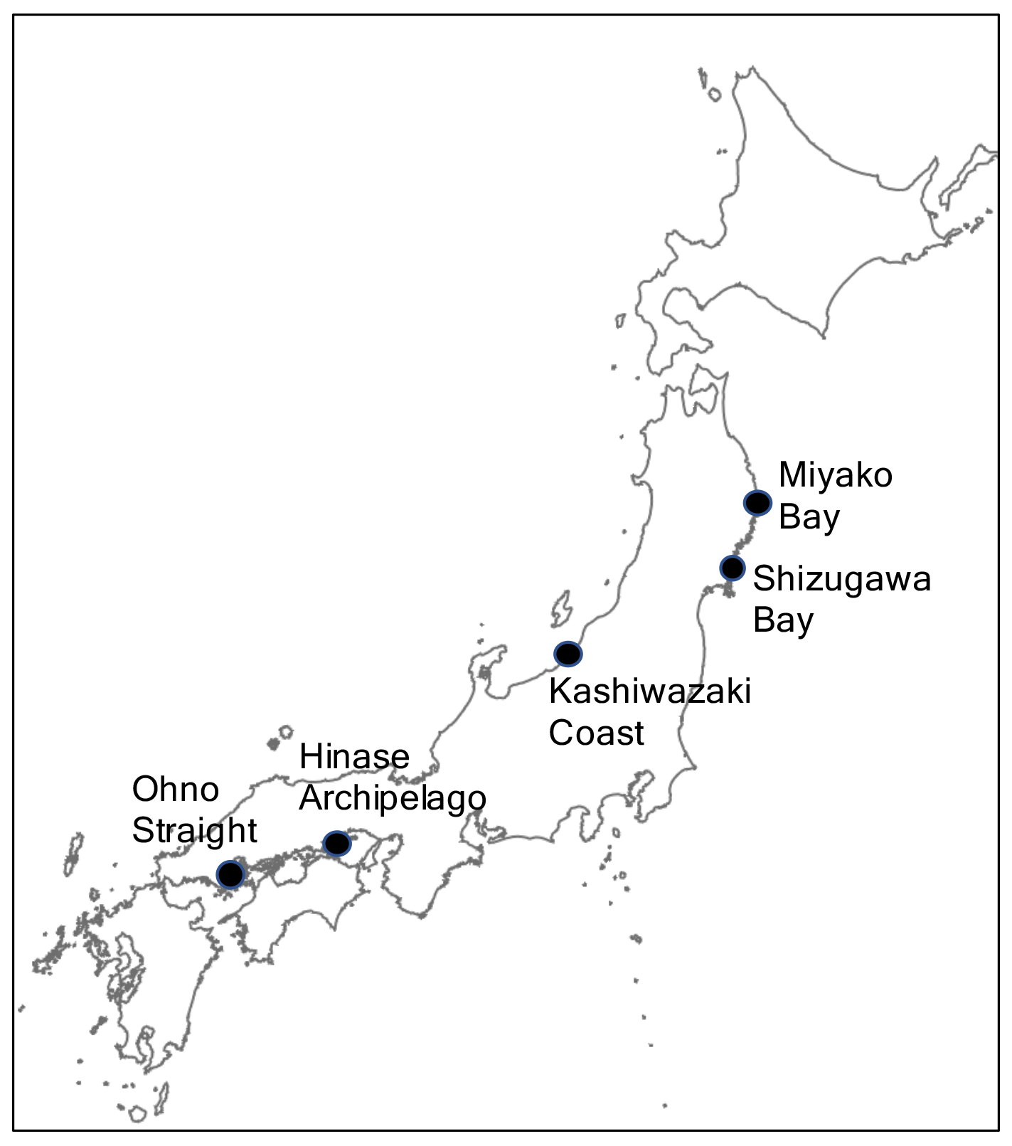
Figure 1Map of the five study stations along the coast of Japan.
2.1 Miyako Bay
Miyako Bay is located in the northern part of Honshu Island facing the western North Pacific, with a bay area of 24 km2 and a 4.8 km wide bay mouth (Fig. 2a). The outer bay area is usually occupied by temperate western North Pacific water, which brings enough nutrients in winter to support seaweed farms in the coastal area (Kakehi et al., 2018). Additional nutrients to the bay are provided by three rivers: Hei, Tsugaruishi, and Tashiro (25.8, 5.16, and 3.78 m3 s−1, respectively, for annual average flow rate; Okada et al., 2014), although the quantity of nutrients input by the rivers are limited to low levels (57, 11, and 8 tN yr−1 for Hei, Tsugaruishi, and Tashiro rivers, respectively; Bernardo et al., 2023). With a population of 60 000 residents within the hinterland, Miyako Bay has maintained good water quality with 1–2 mg L−1 of chemical oxygen demand (MOE, 2022). While kelp beds are well developed near the shoreline, wakame seaweed (Undaria pinnatifida) farmyards are developed in the middle of the bay.
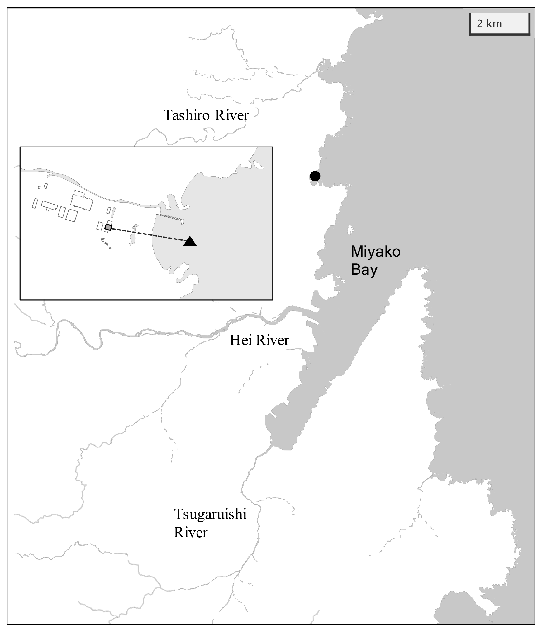
Figure 2Map of Miyako Bay with the location of the station (black circle). Overlaid map shows detailed structure of the station. Gray square and black triangle represent locations of settling tank and water intake, respectively.
The monitoring site was located in front of the Miyako Field Station of the Japan Fisheries Research and Education Agency, which is located north of the bay mouth (141∘58′5′′ E and 39∘41′28′′ N; Fig. 2). This area frequently encounters severe winter storms, so we set the monitoring station in the settling tank (3.6 × 2.8 × 5.4 m) of the field station, in which coastal water is continuously pumped from the water intake located 200 m off the coastline and 1–3 m in depth (Fig. 2). Sensors for pH (SPS-14; Kimoto Electric), dissolved oxygen (DO) (AROW2; JFE Advantech), and salinity/water temperature (ACTW; JFE Advantech) were then moored at a depth of 1 m in the settling tank. Mechanical precision of each sensor is ±0.003 pH units for pH, ±2 % for DO, ±0.008 for salinity, and ±0.01 ∘C for water temperature, respectively. The difference in pH between water intake and settling tank was measured for two weeks during the monitoring period, and it was confirmed that the difference in pH between the water intake and settling tank was <0.006 pH units. The sampling frequency of each sensor was set to 1 h. All sensors were replaced every 2 months because of the limitation of batteries, and the DO sensor was calibrated by air-saturated pure water and sodium sulfite solution, while the pH sensor was calibrated against tris(hydroxymethyl)aminomethane and 2-amino-2-methyl-1-propanol-buffered artificial seawaters provided by FUJIFILM Wako Pure Chemical Corporation (cat. no. 017-28191 and 010-28181, respectively) at the beginning of each deployment. Along with these measurements, discrete water samples were taken from the tank at a depth of 1 m using a 1.5 L Niskin bottle every week. Subsamples for salinity, nutrients, dissolved inorganic carbon (DIC), and total alkalinity (TA) were then taken and stored. Salinity and nutrients were measured at the Yokohama Laboratory of the Japan Fisheries Research and Education Agency using a salinometer (8400 B; Guildline Instruments) and continuous flow analyzer (QuAAtro 39; Seal Analytical), respectively, while DIC and TA were measured at the Mutsu Institute for Oceanography of the Japan Agency for Marine-Earth Science and Technology (MIO-JAMSTEC) using a carbon coulometer (UIC CM 5012 with Nippon ANS model 3000A) and an open-cell titrator (Kimoto Electric ATT-15) calibrated against the seawater reference materials provided by KANSO Corporation (Wakita et al., 2021). Measurement precision was ±1 µmol kg−1 for both DIC and TA. The pH of the seawater at the time of each sampling (pHdiscrete) was calculated from DIC and TA using the CO2sys program v2.1 (Pierrot et al., 2006), with the settings of Lueker et al. (2000) for the dissociation constant of carbonate, Dickson (1990) for the dissociation constant of bisulfate, and Lee et al. (2010) for the aqueous boron concentration. The drift of the pH sensor during deployment was corrected based on the difference between pHdiscrete and the pH measured by the sensor. The relationship between the measured TA and salinity was evaluated as a linear function, and the time series of TA throughout the sensor deployment was calculated based on the salinity–TA relationship. The saturation states of aragonite (Ωar) were then calculated from water temperature, salinity, nutrient concentrations, DIC, and TA using the CO2sys program. This monitoring program, founded by the Study on Biological Effects of Acidification and Hypoxia (BEACH) of the Environment Research and Technology Development Fund of the Environmental Restoration and Conservation Agency, started on 1 July 2020 and ended on 21 September 2021.
2.2 Kashiwazaki Coast
Kashiwazaki City is located at the center of Honshu Island facing the Sea of Japan. Its coastline has little flexure, with the periodic occurrence of shallow sandy beaches and small rocky reefs (Fig. 3a). While benthic biomass is quite low in sandy beach coastal areas, local Sargassum seaweed beds are formed off rocky reefs. The low-nutrient Tsushima Warm Current flows throughout the year off the narrow band of low-salinity coastal water (Niigata Prefectural Institute for Fisheries and Oceanography, 1998). Kashiwazaki City has a population of 79 000 with a cultivated land area of 4890 ha (mainly rice paddy fields) and ∼ 200 plants of manufacturing industries. Sewage waters from these civil activities are released into coastal areas via two small rivers, Sabaishi and Ukawa, which bring low salinity and nutrients. The quality of off-Kashiwazaki coastal waters has been well maintained, with a chemical oxygen demand of <2 mg L−1 (MOE, 2022). However, 30 years of monitoring by the Marine Ecology Research Institute shows that the pH of off-Kashiwazaki coastal water has decreased at a rate of −0.003 yr−1 because of the increase in water temperature and concentration of atmospheric CO2 (Ishida et al., 2021).
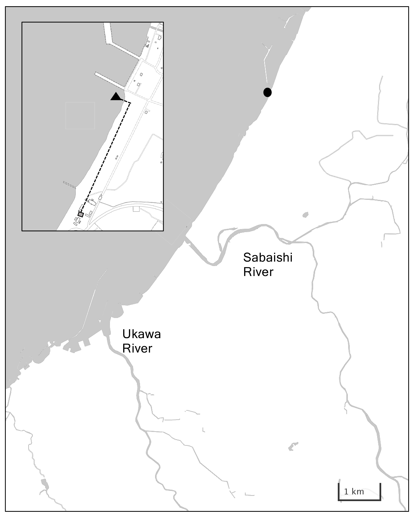
Figure 3Panel (a) shows a detailed map of Kashiwazaki Coast with the location of the station (black circle), and (b) shows locations of water intake and the settling tank in Kashiwazaki Observatory.
Similar to the Miyako site, sensors for pH, DO, and salinity/water temperature were set within the water tank (3000 L), to which coastal water was continuously pumped from the water intake set in front of the Marine Ecology Research Institute (138∘35′24′′ E and 37∘25′30′′ N; Fig. 3b). The settings of each sensor, water sampling, and measurements were the same as those of the Miyako site. This monitoring program, also founded by BEACH, started on 16 July 2020 and ended on 24 August 2021.
2.3 Shizugawa Bay
Shizugawa Bay is located ∼ 100 km south of Miyako Bay, with a bay area of 46.8 km2 and a 6.6 km wide bay mouth (Fig. 4). The Oyashio-oriented cold-water and Kuroshio-oriented warm-water masses intermittently occupy the outer bay, and the former water brings high quantities of nutrients to this bay in winter, similar to that in the Miyako Bay. The large Kitakami River (water transport of 390 m3 s−1), flows out to the sea south of Shizugawa Bay, bringing nutrients of 6 × 10³ tN yr−1 to the coastal area (Sugimura et al., 2015). In addition, 10 small rivers flow directly into the bay and the total nutrient flux provided by these rivers was estimated at 270 tN yr−1 (Yamamoto et al., 2018). Shizugawa Bay has been widely used for the aquaculture industry, especially for culturing Pacific oysters and silver salmon. Historically, the extent of aquaculture utilization occasionally becomes too heavy, resulting in the emergence of low-oxygen deep waters in the bay caused by the degradation of organic materials derived from aquaculture. After the Great East Japan Earthquake in 2011, oyster farmers in Shizugawa Bay decided to reduce the number of their oyster rafts to one-third of what they had before the earthquake to reduce the environmental impact of aquaculture on the bay ecosystem, which was on the way to recovery from the tsunami disaster. As a result, the DO of the bottom water in the bay showed a remarkable increase by >1 mg L−1 (Yamamoto et al., 2017).
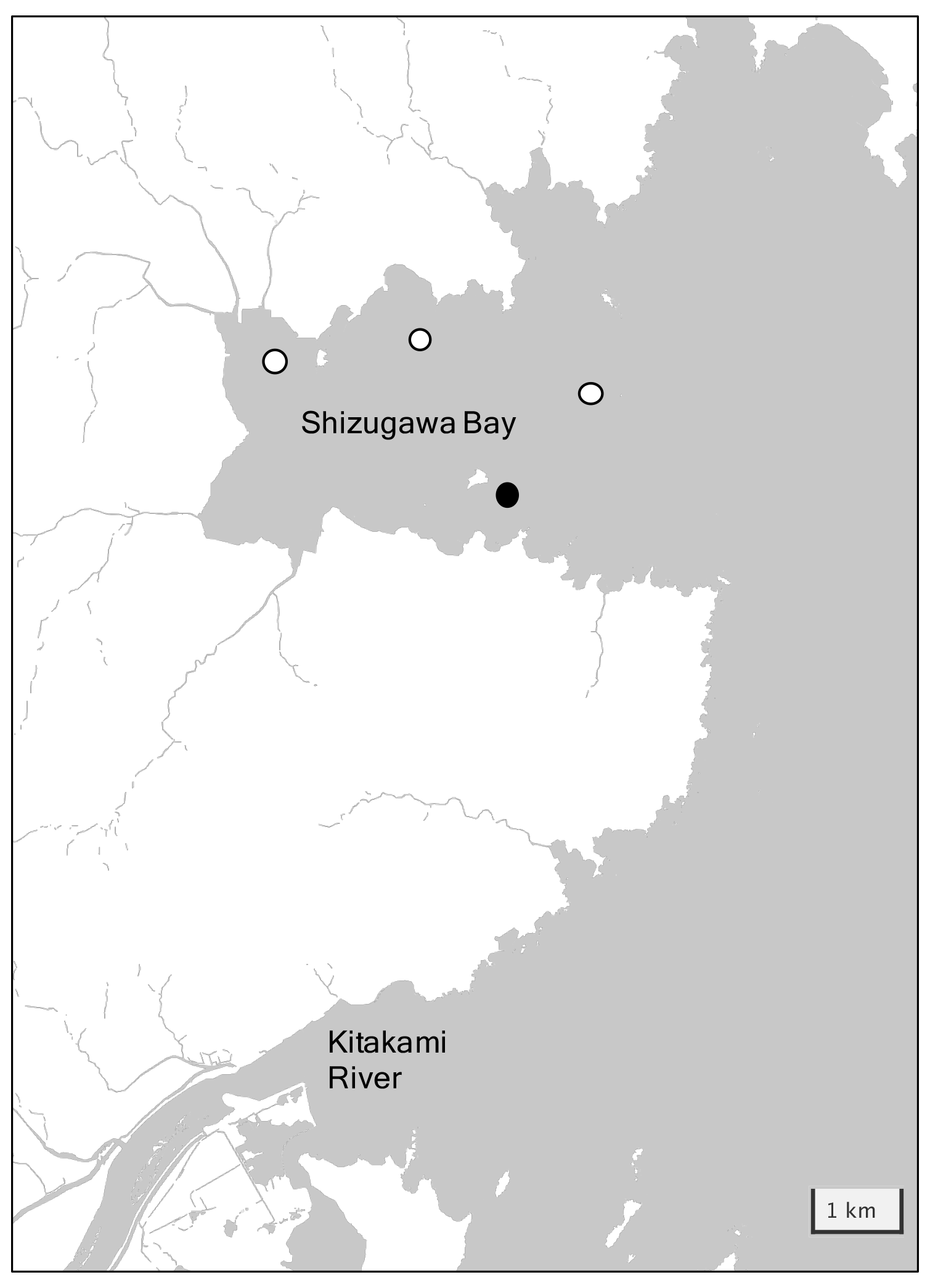
Figure 4Detailed map of Shizugawa Bay with the location of the station. The white circles represent stations installed by the Ocean Acidification Adaptation Project and the black circle represents the location of station S3 used in this study.
Since 2020, hydrographic conditions, including pH, have been observed at four stations within Shizugawa Bay (Fig. 4) by the Ocean Acidification Adaptation Project (OAAP) founded by the Nippon Foundation (Fujii et al., 2023). Detailed settings of the observations are described in Fujii et al. (2023), and here, we reproduce its brief outline: sensors for water temperature, salinity, DO, and pH were set at a depth of 1 m in each station to collect data at a temporal resolution of 1 h. Water samples for salinity, nutrients, DIC, and TA were taken from each station monthly, and the sampling interval was enhanced to every 15 d during summer. Salinity, nutrients, DIC, and TA were measured by the same methods as for the Miyako site, although measurements were made at the Kesen-numa Laboratory of Miyagi Prefectural Institute for Fisheries Sciences and MIO-JAMSTEC for nutrients and other properties, respectively. Similar to the Miyako site, pHdiscrete was calculated from DIC and TA and used for the drift correction of the pH sensors. The time series of TA throughout the sensor deployment was also calculated based on the observed TA–salinity relationship. In this study, we used data from Station S3 (Fig. 4) as a representative of Shizugawa Bay, as this station is located in oyster farming areas, the largest aquaculture industry, which is the largest source of organic carbon in this bay. The measurement of water temperature, salinity, and pH was started on 20 August 2020 and that of DO on 27 April 2021. All parameters are continuously measured to date; however, we use data from August 2020 to December 2021 to maintain synchronicity with data of other stations.
2.4 Hinase Archipelago
The Seto Inland Sea is the largest inner sea in Japan (∼ 2.32 × 10⁴ km2) surrounded by the Honshu, Shikoku, and Kyushu Islands, and the Hinase Archipelago is located in the middle of the Seto Inland Sea. This area consists of four major waterways and many small canals divided by Honshu Island and eight other small islands with a water depth of ∼ 6 m (Fig. 5). The Seto Inland Sea is a moderately eutrophic area, receiving 53.0 km3 yr−1 of freshwater and 1.41 × 10⁵ tN yr−1 of nitrate from the surrounding lands (Higashi et al., 2018; Nishijima, 2018). The water exchange rate between the Seto Inland Sea and the outer North Pacific is also high (residence time of ∼ 8 months; Yanagi and Ishii, 2004), and as a result, the nutrient concentration of surface water in the Seto Inland Sea is maintained at a moderate level (∼ 0.4 µM of DIN near the Hinase Archipelago; Tsukamoto and Yanagi, 1998). Historically, nutrient loading was the highest in the 1980s (∼ 2.35 × 10⁵ tN yr−1; Nishijima, 2018). While the long-standing efforts of local communities succeeded in reducing it to the current level, significant quantities of organic nutrients still remained in the bottom sediment, creating local internal sources of nutrients in the Seto Inland Sea (e.g., Yamamoto et al., 2021). Although there is no large point source of nutrients, such as chemical plants, near the Hinase Archipelago, this area also receives nutrients from the Bizen city, which has a population of 36 000 residents. The Chikusa River, with an average flow rate of 33.5 m3 s−1, flows in the eastern edge of this area, while several other small streams provide additional freshwater. The coastal area of the southern Hinase Archipelago is filled with eelgrass beds, while the northern coastal areas are partially filled with artificial shorelines, such as port facilities and breakwaters. Oyster aquaculture is widely used in open water areas. The OAAP also launched four stations in this area (Fig. 5). Settings of sensors, water sampling, and its measurements were the same as those of Shizugawa Bay, with the exception that nutrient measurements were done by the Okayama Prefectural Institute of Fisheries Sciences (see Fujii et al., 2023 for details). In this study, we used data from Station H2 (Fig. 5) to represent the Hinase Archipelago, as this station is located in the center of oyster farming areas. Measurements of water temperature, salinity, and pH were started on 29 August 2020, while measurements of DO were started on 10 June 2021. All parameters are continuously measured to date; however, we use data from August 2020 to December 2021.
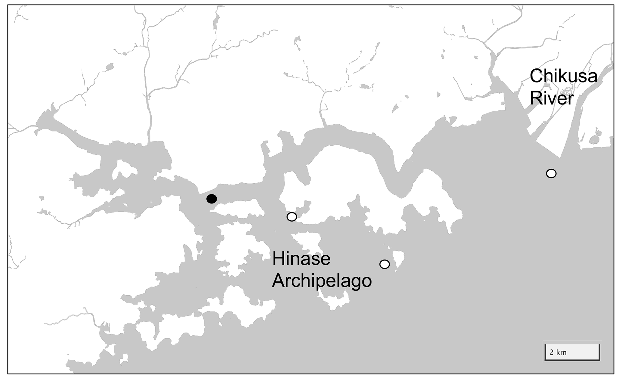
Figure 5Detailed map of Hinase Archipelago with the location of the station. The white circles represent stations installed by the Ocean Acidification Adaptation Project and the black circle represents the location of station H2 used in this study.
2.5 Ohno Strait
Ohno Strait is the small strait between Honshu and Miyajima islands, which are located at the southern boundary of Hiroshima Bay in the western Seto Inland Sea (Fig. 6). As part of the Seto Inland Sea, the surface water surrounding Ohno Strait is moderately eutrophic (∼ 2 µM of DIN; Tsukamoto and Yanagi, 1998), although it is slightly lower than the Hinase Archipelago, reflecting an east–west gradient of surface nutrient concentration. The Ohta River, which flows through Hiroshima city with a population of 1.2 million, adds 1.93×10³ tN yr−1 of nitrogen into Hiroshima Bay (Yamamoto et al., 2002). Part of the Ohta River water plume flows into the Ohno Strait (Abo and Onitsuka, 2019), providing nutrients to the surface layer of this strait. Industrial areas with a population of 115 000 are developed along the western coast of this strait, providing another nutrient source to this area. The strait itself is lightly used for oyster farming and the bottom sediment in the strait is mainly filled by silt and shell fragments.
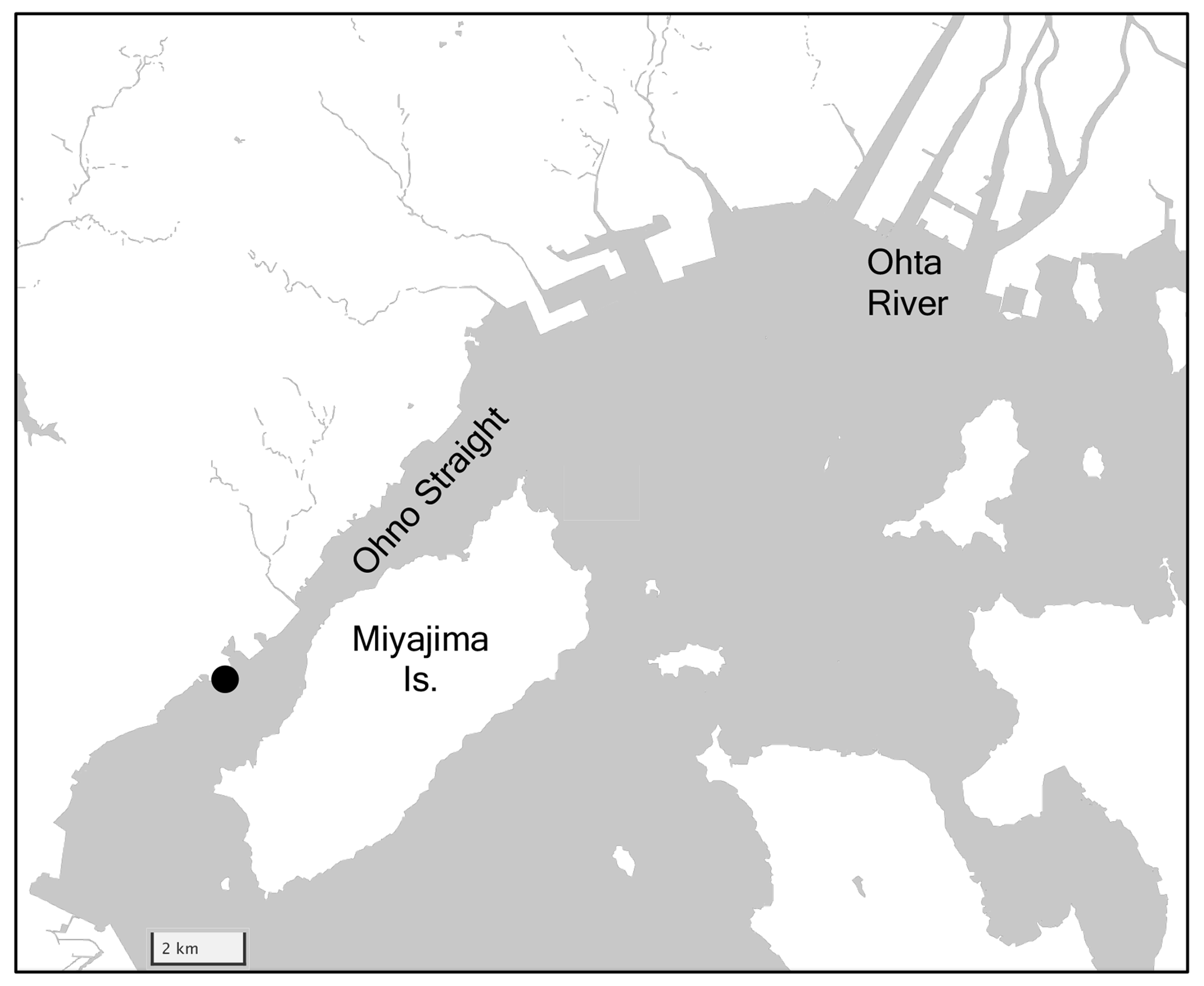
Figure 6Detailed map of Ohno Strait with the location of the station (black circle).
The monitoring station was launched in the experimental raft off the Hatsukaichi Field Station of the Japan Fisheries Research and Education Agency, with a water depth of 3–6 m depending on the tide. A set of sensors (SPS-14 for pH, Kimoto Electric; AROW2 for DO, JFE Advantech; and ACTW for salinity/water temperature, JFE Advantech) were fixed from the raft at a depth of 1 m, and each parameter was measured at an interval of 1 h. The methods and frequencies for sensor calibration and discrete water sampling were the same as those of the Miyako site. This station was launched on 22 June 2021 by the OAAP and is continuing to operate to date; however, we used data from June 2021 to December 2021.
3.1 Temporal variation in water temperature, salinity, and DO
Figure 7 shows the time series of water temperature, salinity, and DO at the five stations. All stations showed similar seasonal variations in water temperature, with the highest and lowest temperatures in July and February, respectively (Fig. 7a). The seasonal amplitude was the largest in Hinase and the smallest in Miyako. At all stations, water temperature showed significant day-to-day variation with a timescale of <10 d and also diurnal variations. We discuss this further in Sect. 4.1.
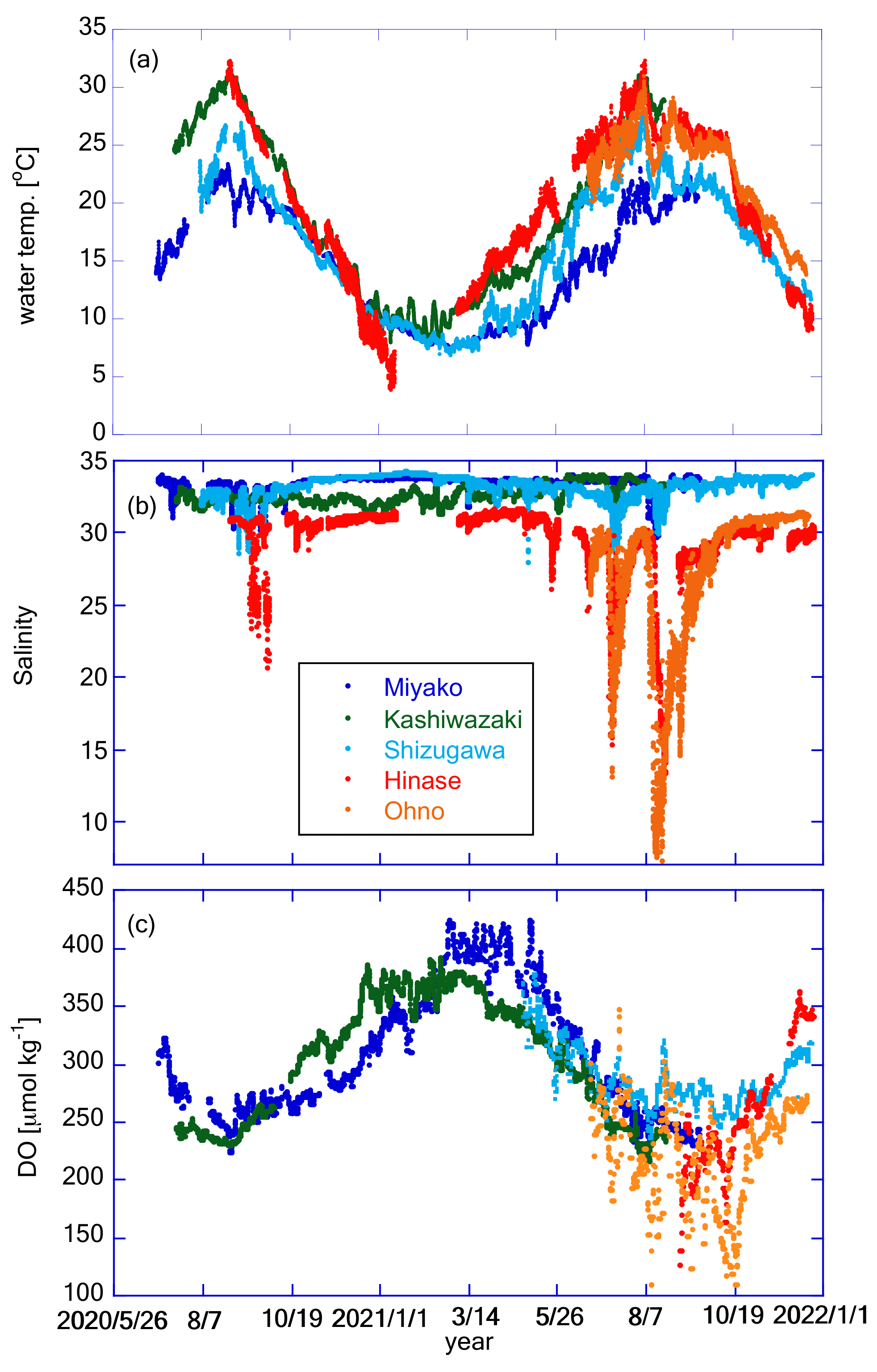
Figure 7Time series of (a) water temperature, (b) salinity, and (c) DO at the five stations. Legends of color plots are the same for all panels as shown in (b).
Time series of salinity in Shizugawa, Hinase, and Ohno show similar patterns of seasonal variation, low in summer/autumn and high in winter (Fig. 7b), suggesting that the main source of freshwater in these areas are rainfall events (during the rainy season in June–July and typhoon season in August–October). In contrast, in Kashiwazaki, salinity is high in summer and low in winter, suggesting that the main freshwater source in this area is snowfall in winter. The salinity of the Miyako site shows two low-salinity peaks, one in spring and the other in autumn, suggesting that this area is affected by both snowmelt waters and typhoon events (JFA, 2004). In Miyako, Shizugawa, Hinase, and Ohno, where the freshwater input is significant in summer/autumn, salinity frequently showed short-term drawdown that is synchronized with local rainfall events. The amplitude of sporadic salinity drawdown was extremely large in Hinase and Ohno, where the surface salinity temporally reached to less than 10 (Fig. 7b). Amplitude of seasonal annual variation in these two areas reaches over 25, which corresponds to the largest annual salinity amplitude among the world's 83 stations collected in Carstensen and Duarte (2019). We discuss the effect of these short-term low-salinity events on pH in Sect. 4.3.
DO showed similar patterns of seasonal variation: low in summer and high in winter, although the durations were short in Hinase and Ohno (Fig. 7c). This pattern suggests that the seasonal variation in DO is mainly driven by variation in oxygen solubility induced by water temperature rather than biological processes (see Sect. 4.2 for more details). This seasonal variation overlaps with day-to-day variation with a duration of ∼ 10 d, and the amplitude of such day-to-day variation is especially significant in Hinase and Ohno in summer and autumn. Because of this short-term day-to-day variation, DO in Hinase and Ohno were occasionally below 150 µmol kg−1 in summer and autumn, indicating that water conditions in these two areas occasionally become significantly undersaturated in DO, even in surface waters.
3.2 Temporal variation in pH
Figure 8a shows the time series of pH after drift correction at five stations. (Hereafter, all pH values are reported in total scale in this paper.) Although the mechanistic precision of the pH sensor is ±0.003 pH units, the uncertainty of the pH value measured by the glass electrode is mainly controlled by the precision of its drift correction. In the case of Miyako, where drift correction was performed weekly, we set two pH sensors in the same settling tank for 2 weeks to evaluate the reliability of pH data after the drift correction process. Values of pH obtained from the two sensors matched with that of 2 standard deviations (SD) of ±0.010 pH units, and we used this value as the uncertainty of pH values obtained at Miyako, Kashiwazaki, and Ohno stations. In Shizugawa and Hinase, drift corrections were made at longer intervals, and Fujii et al. (2023) evaluated the uncertainty of pH at these two stations at ±0.015 pH units. Figure 8a shows significant daily fluctuations far higher than these pH uncertainties. The diurnal amplitude was the largest in winter in Shizugawa Bay, where the difference in pH between day and night exceeded 0.8 pH units. Large diurnal variations in pH and/or pCO2 are often measured in shallow coastal ecosystems (e.g., Fujii et al., 2021; Ricart et al., 2021; Waldbusser et al., 2014). In most cases, large diurnal pH variation is observed in summer, and the largest diurnal amplitude of pH in winter has rarely been reported. Such patterns raise the possibility of biofouling in pH sensors (e.g., Venkatesan et al., 2017), although visual inspection at the time of sensor exchange did not show significant adherence of biomes during winter. However, the detailed pH variation in each day (Fig. 8b) showed that during the night it was relatively low and constant, even during significant diurnal variation. This is probably because the organic material produced by the fouling biomes during the day had settled down from the sensors, and hence, the effect of the decomposition of organic materials during the night remained low even in the large diurnal variation period. We do not further discuss diurnal variations of pH, as we do not have definite evidence for the effect of biofouling in winter in Shizugawa Bay. We alternatively calculated the daily minimum pH (pHmin), which is usually observed at night, and analyzed the day-to-day variation in pHmin at various timescales (Fig. 8c). Several rearing experiments have suggested that coastal organisms are affected by pHmin rather than the daily average pH (e.g., Onitsuka et al., 2018); therefore, the daily variation in pHmin was analyzed instead of pH.
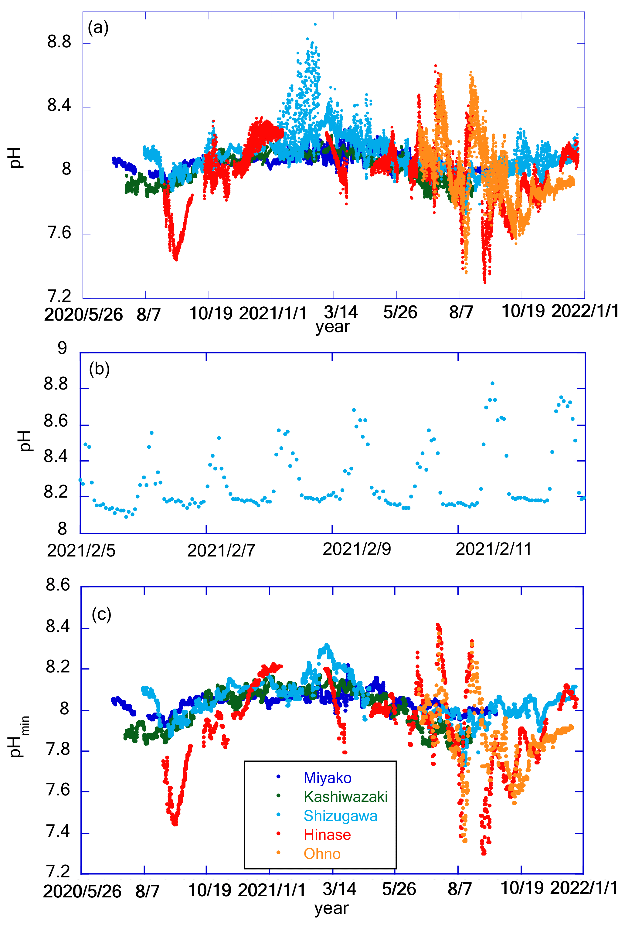
Figure 8Panel (a) shows time series of pH in each station. Panel (b) shows an example of detailed pH time series. Data in Shizugawa Bay from 2 to 9 February 2021 are presented here. Panel (c) shows time series of pHmin in each station. Legends of color plots are the same for all panels as shown in (c).
pHmin showed a similar pattern of seasonal variations at all five stations, with high values in winter and low values in summer/autumn (Fig. 8c). Seasonal amplitude was the smallest in Miyako and the largest in Hinase and Ohno (Fig. 7a). In Hinase and Ohno, the annual range of pHmin variation reached over 1.1 pH units, which was larger than that of 83 stations around the world listed in Carstensen and Duarte (2019) except for the Baltic Sea. This seasonal variation overlapped with the short-term drawdown event of pHmin, which was frequently observed in summer/autumn. The timing of such events was synchronized with that of short-term low-salinity events (Fig. 7b). This result indicates that either rainfall or increased river flow causes several short-term processes in these coastal areas, causing short-term variation in pH.
3.3 Relationship between TA and salinity
Figure 9 shows the observed relationship between TA and salinity based on discrete water samples obtained at each station. TA in Miyako, Kashiwazaki, and Shizugawa varied in a narrow range between 2222 and 2236 µmol kg−1 at a salinity of 33.5, which is approximately equal to that in the surface waters of the western North Pacific in the corresponding latitudinal range (Takatani et al., 2014). This similarity of TA range indicates that coastal waters in these three areas are occasionally not significantly different from their open water sources when salinity is satisfactorily high (∼ 33.5). In contrast, in Hinase and Ohno, we obtained TA of 2222 and 2182 µmol kg−1, respectively, if we extended their regression equation to a salinity of 34.0. These values again fit with those of Kuroshio waters (Takatani et al., 2014), reflecting that the ultimate source water for the Seto Inland Sea is Kuroshio. It is noteworthy that the maximum salinity values observed in Hinase and Ohno were 31.67 and 31.43, respectively (Fig. 7b). These results indicate that the open waters of the Hinase and Ohno areas are already diluted from their ultimate source (i.e., Kuroshio water), and hence, have already witnessed several modifications through coastal processes within the Seto Inland Sea.
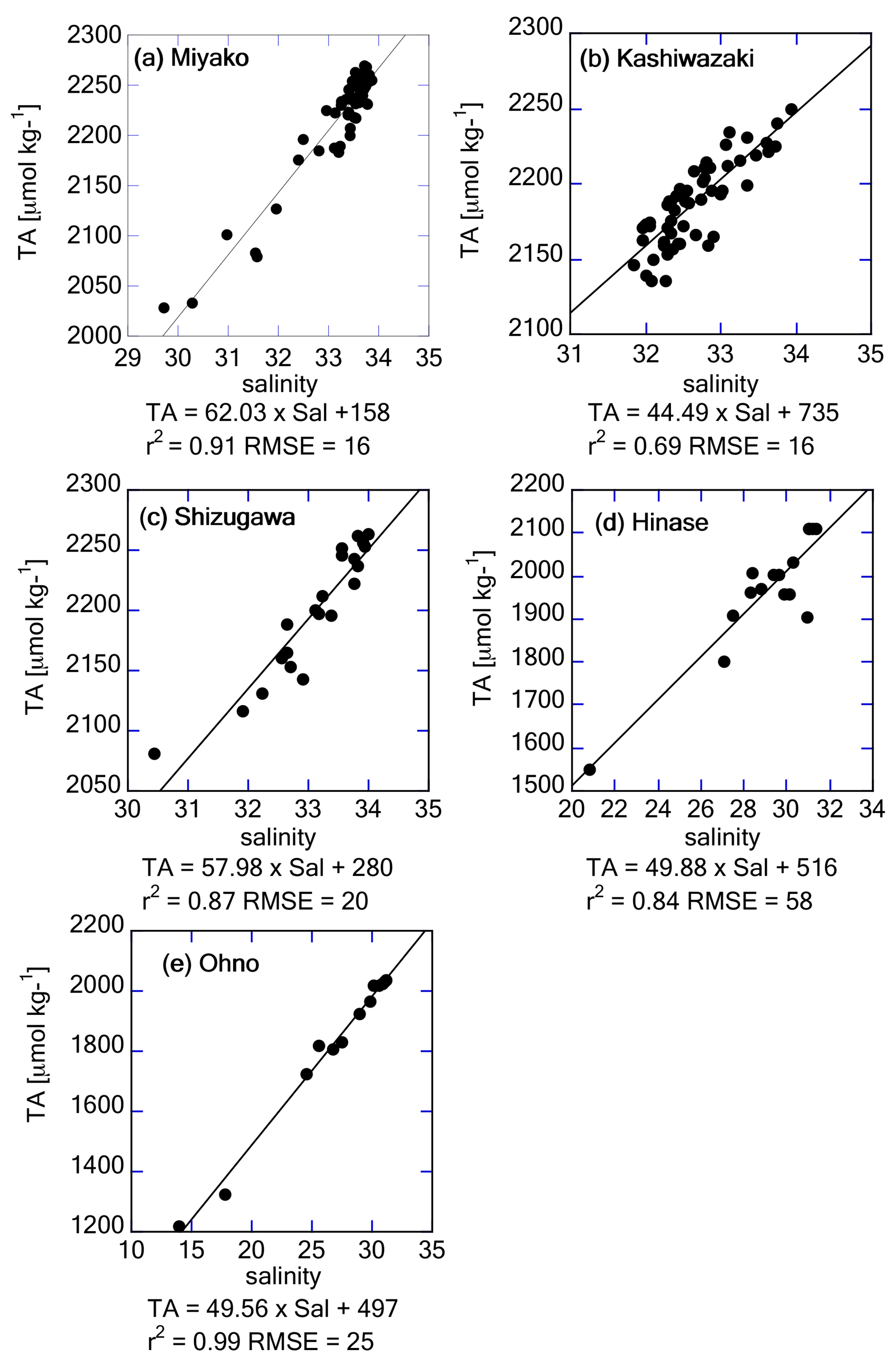
Figure 9Salinity–TA relationship based on discrete water samples obtained from (a) Miyako, (b) Kashiwazaki, (c) Shizugawa, (d) Hinase, and (e) Ohno stations. Regression equations are provided below the x axes.
The freshwater endmember in each regression line represents the TA of the main freshwater source in each area, although the absence of a low-salinity data point leads to a high uncertainty in estimating the endmember. Table 1 describes the list of TA at the mouth of the major freshwater inflow in each coastal area. In most study areas, the calculated freshwater endmember of TA-S regressions agreed with the observed TA of one of the freshwater sources (Table 1), indicating that non-dilution/concentration changes in TA (Jiang et al., 2014) were relatively small in these areas, and by comparing these values with the freshwater endmember calculated from Fig. 9, we can speculate which river was the actual major freshwater source for each area. For the Miyako station, which is located at the northern edge of Miyako Bay, the Tashiro River becomes a major controller of salinity because of its proximity to the station. Two small rivers are neighboring the Kashiwazaki site and both rivers can act as salinity controllers for this site based on TA. Interestingly, all small rivers that flow into Shizugawa Bay had far higher TA than the calculated freshwater endmember, reflecting the existence of limestone areas in their basin. Rather, the TA of Kitakami River, despite flowing into a different bay south of Shizugawa, fitted with that of the freshwater endmember, suggesting that this river is the main source of freshwater for Station S3 because of its large flow rate. In the Hinase Archipelago, all surrounding rivers had similar TA, and hence, we cannot determine which rivers are the main freshwater sources for Station H2. The freshwater endmember calculated in Ohno Strait was significantly higher than the TA of its neighboring large river (Ohta River), suggesting an additional contribution from small rivers directly facing this strait.
Table 1Total alkalinity (TA) of freshwater sources in each coastal area, with calculated TA of freshwater endmember from the salinity–TA relationship (see Fig. 9). Uncertainty terms of freshwater endmember was calculated as standard error of sal = 0 intercept in least squares fitting.
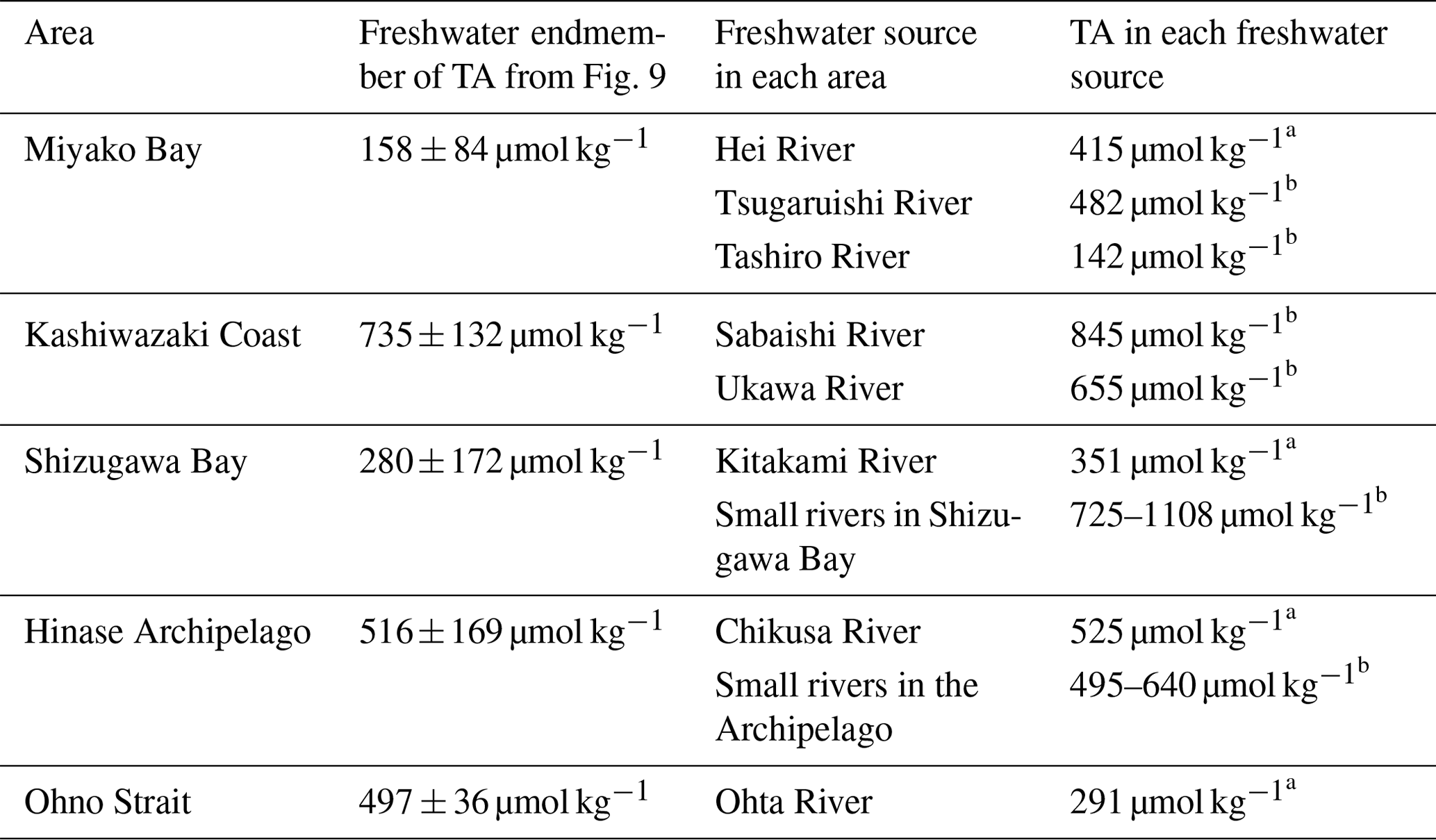
a Values from Kobayashi (1960). b Measured in this study.
3.4 Temporal variation in parameters derived from pHmin and TA
Based on the regression equation obtained from Fig. 9, we calculated the time series of TA from the time series of salinity at each station (Fig. 10a). We then calculated the time series of DIC, pCO2, Ωar, and Ωca from pHmin and TA, and here, we show the results of pCO2 and Ωar in Fig. 10b and c. In this calculation we used time series of pHmin and TA estimated from salinity, and uncertainty of these parameters were of the order of ±0.010 pH units and ±20 µmol kg−1 for pHmin and TA, respectively (see Sects. 3.2 and 3.3 for details). Uncertainty of derived parameters by using these values were estimated by using CO2sys program as ±15 µatm and ±0.07 for pCO2 and Ωar, respectively.
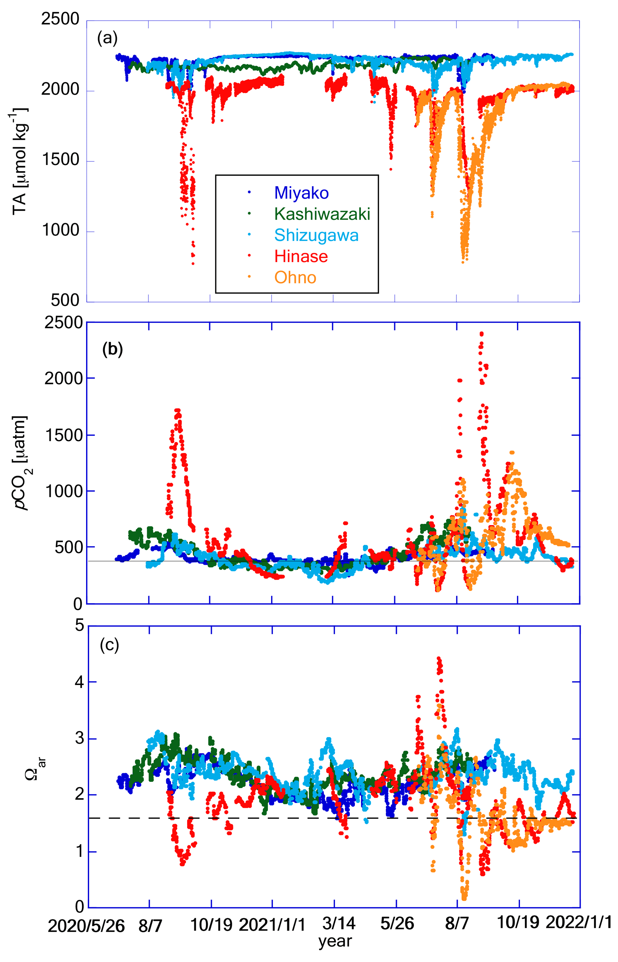
Figure 10Time series of (a) TA, (b) pCO2, and (c) Ωar at the five stations. Legends of color plots are the same for all panels as shown in (a). The solid line in (b) represents the pCO2 value in equilibrium with the present atmospheric CO2 concentration of 416 ppm. The dashed line in (c) represents the experimentally obtained threshold of the ocean acidification effect for the larvae of Pacific oyster Crassostrea gigas (Ωar=1.5; Waldbusser et al., 2015).
Since TA was calculated as a linear equation of salinity, it was expected to have a resemblance between the TA and salinity patterns (Fig. 10a). Sporadic decreases in TA corresponding to low-salinity events in Hinase and Ohno were noticeable. Water with low TA has low buffer capacity, and hence, it has particularly high risks of low pH and high pCO2 (e.g., Carstensen and Duarte, 2019; Salisbury et al., 2008). Figure 10b shows an appearance of such risk, extremely high pCO2 over 1500 µatm during the low-salinity period in Hinase and Ohno. The annually averaged pCO2 values were 404, 450, 393, 589, and 621 µatm for Miyako, Kashiwazaki, Shizugawa, Hinase, and Ohno, respectively, showing that surface waters are in equilibrium with or even higher than current atmospheric concentration of CO2 (416 ppm at 2021; WDCGG, 2024). Generally, estuary areas tend to become sources of atmospheric CO2, while “open” coastal areas, such as marginal seas, continental shelves, and large bays, tend to become sinks of atmospheric CO2 (e.g., Borges et al., 2005; Kubo et al., 2017; Laruelle et al., 2010; Tokoro et al., 2020). Typically, terrestrial input of organic matter from rivers is mostly decomposed in estuaries, causing high pCO2 and low pH, as well as a high nutrient flux to the outer estuary. In an “open” coastal area, nutrients transported from the estuary activate high primary production, which causes low pCO2 and high pH in surface waters. The Seto Inland Sea itself is considered a sink of atmospheric CO2 (e.g., Tokoro et al., 2020), and hence, it can be treated as an open coastal area. Our results indicate that despite the high distance from the large river mouth, both Hinase Archipelago and Ohno Strait can be classified as “estuaries”, or at least as areas that receive a significant quantity of particulate organic matter from land.
The Ωar was high in summer and low in winter in Miyako, Kashiwazaki, and Shizugawa (Fig. 10c), showing an opposite pattern to the seasonal variation in pHmin. This was due to the large seasonal variation in the solubility of aragonite induced by the seasonal change in water temperature (see Sect. 4.2). In contrast, in Hinase and Ohno, the amplitude of seasonal variation in pH was large enough to overcome seasonal variation in aragonite solubility, and as a result, Ωar changed to show a seasonal maximum in winter and a seasonal minimum in summer. Short-term variation in Ωar linked to that of salinity also overlapped with seasonal scale variation, and as a result, significantly low Ωar conditions were frequently observed in Hinase and Ohno. Fujii et al. (2023) described that during summer–autumn in the Hinase Archipelago, Ωar occasionally falls below the threshold level of the larvae of the Pacific oyster Crassostrea gigas, with the effect of ocean acidification (OA) becoming detectable in the rearing experiment (∼ Ωar=1.5; Waldbusser et al., 2015). This study showed that the situation was almost the same in Ohno Strait (Fig. 10c). It should be highlighted that Fujii et al. (2023) also noted that actual damaged larvae were not detected based on microscopic inspection of Hinase (n=1062). The rearing experiment of Waldbusser et al. (2015) was conducted on the Oregon coast (USA), where C. gigas is non-native. Therefore, it is not unrealistic that there is a difference in the tolerance for OA between the local population of Oregon and Seto Inland Sea, the latter being the native habitat of C. gigas. Kurihara et al. (2007) examined the effect of low pH in the Seto Inland Sea population of C. gigas, and found that the larvae of this population are affected by OA at a pH of 7.4 (National Bureau of Standards (NBS) scale). This threshold approximately corresponds to a pH of 7.27 in the total scale, and in this case, larvae of Pacific oysters are considered to be safe in most seasons both in Hinase and Ohno (Fig. 8c). In the experiment by Kurihara et al. (2007), the rearing experiment was occupied only at the control (pH of 8.2 in the NBS scale) and acidified (pH of 7.4 in the NBS scale) conditions, and hence, a true threshold for the Seto Inland Sea Pacific oyster population can exist between a pH of 7.27 and 8.07. We thus need further studies, including new rearing experiments, to determine why Pacific oyster larvae are still safe in the present Hinase Archipelago.
A low Ωar level (below 1.5) was also detected in Shizugawa Bay (Fig. 10c; Table 2; Fujii et al., 2023) and Miyako Bay (Fig. 10c; Table 2), but its duration was only 4 d and 1 d, respectively, throughout the study period. In Kashiwazaki, Ωar was above this level throughout the observation period. Other calcifiers that are important for fisheries around the Japanese coast, such as Ezo abalone (Haliotis discus hannai) and short-spined sea urchin (Strongylocentrotus intermedius), have lower Ωar thresholds than that of Pacific oyster: 1.1 for H. discus hannai (Onitsuka et al., 2018) and 1.12 for S. intermedius (Zhan et al., 2016). Therefore, Shizugawa Bay, Miyako Bay, and Kashiwazaki Coast have a low risk of OA, at least from the viewpoint of fisheries. However, note that we have investigated only a few marine species so far, and there may be many unknown species that are vulnerable to low pH/low Ωar conditions. We must enhance our knowledge of biological responses according to species, especially for those with low economic importance, such that we can evaluate the total risk posed by OA to the coastal ecosystem.
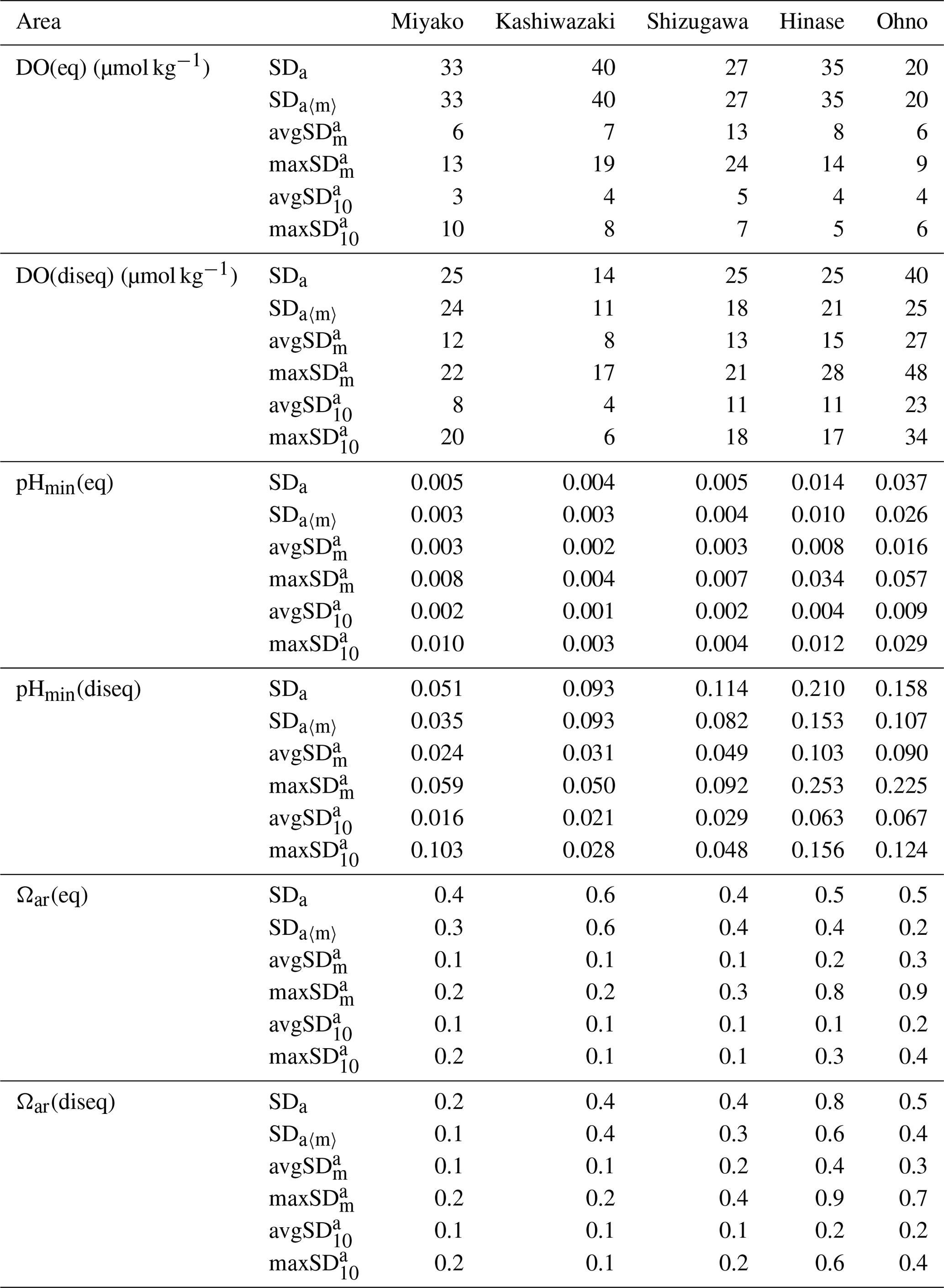
Table 2Statistical aspects of environmental parameters in each station. Annual values are calculated based on the previous 1 year of data to avoid biases that come from different time lengths. See Appendix A for the abbreviation of each SDs with different timescales.
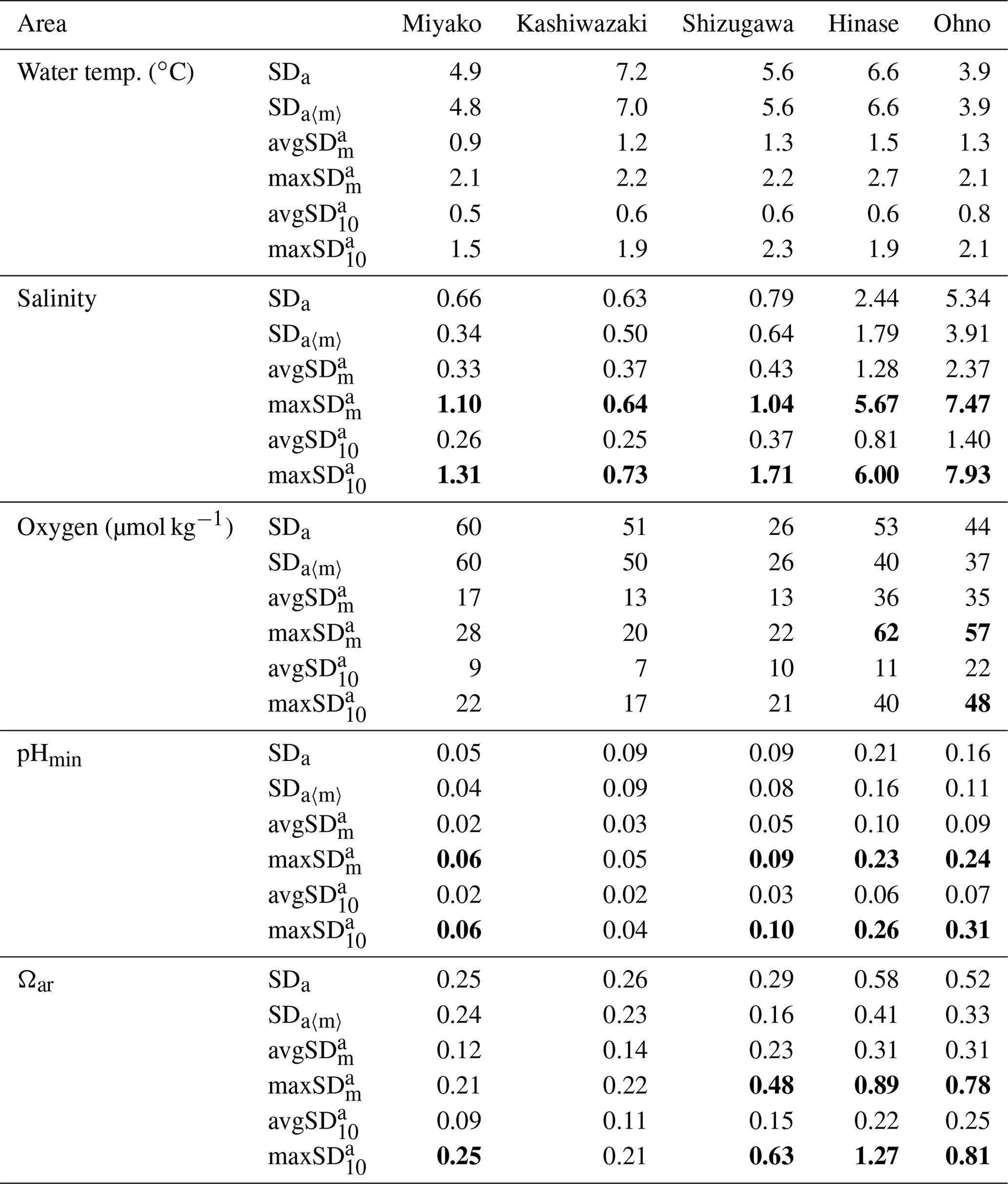
Numbers are shown in bold when they exceed SDa.
4.1 Quantification of short-term variability in properties of water
We focused on short-term variations of pH and related parameters with timescales shorter than 1 month, which cannot be detected by regular MOE monitoring based on water sampling. To assess this quantitatively, we calculated the SD of each parameter at different timescales (annual, monthly, and 10 d). See Appendix A for the abbreviation of each calculated SDs.
The results are listed in Table 2. As shown in Figs. 7 and 9, both the amplitude and frequency of short-term variation differed significantly among the seasons for almost all parameters. To determine seasonal differences in the extent of short-term variation, avgSD in each month is listed in Table 3.
Table 3Monthly average of 10 d standard variation (avgSD) for each parameter in each month in each station. Numbers displayed in bold represent annual maximum and the second maximum.
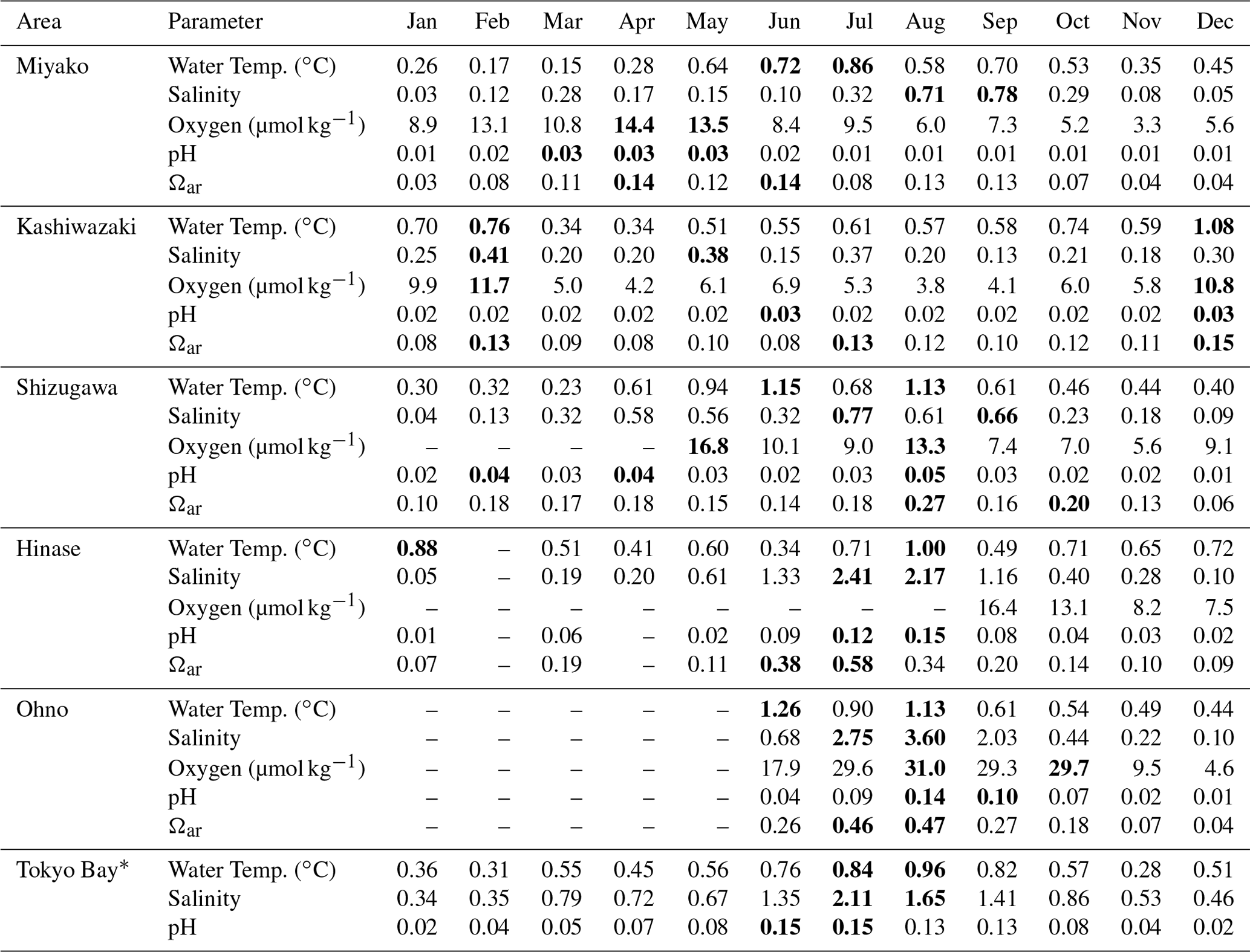
* See Sect. 4.3 for details of the data in Tokyo Bay.
The SDa〈m〉 of water temperature was in the range of 3.9–7.2, and this was almost the same as that of SDa (Table 2). This implies that a large timescale variation of over 1 month (e.g., seasonal scale) was the main component of observed annual temporal variation (Fig. 7a). The avgSD of water temperature (0.9–1.5) was <25 % of the SDa (3.9–7.2), and the avgSD (0.5–0.8) was approximately half of avgSD in each area (Table 2). In the case of salinity, on the other hand, SDa〈m〉 (0.34–3.91) was about 70 % of SDa (0.63–5.34), indicating that variations with a shorter timescale than 1 month contribute some parts of annual variation in the case of salinity. The avgSD of salinity (0.33–2.37) was approximately half of the SDa (0.66–5.34) in each area, and avgSD (0.26–1.40) was approximately two-thirds of avgSD. Seasonal variability of avgSD was also higher than that of water temperature (Table 3), and as a result, avgSD of salinity occasionally exceeded the SDa in several months. Interestingly, avgSD and avgSD were almost the same in Miyako, Kashiwazaki, and Shizugawa (Table 2), and the maxSD for salinity was higher than the maxSD. Such a result can be attributed to the perturbation of salinity that mainly occurs within the timescale of 10 d, and monthly SD of salinity is essentially determined by the amplitude and frequency of 10 d salinity variation included within that month. Although the avgSD of salinity was lower than the avgSD in Hinase and Ohno, the maxSD was still higher than the maxSD, indicating that the 10 d variation is also an influential component of monthly variation in these two areas.
The relative contribution of short-term variation to annual variability for other parameters varied between the above two extremes (water temperature and salinity). In the cases of DO and pH, SDa〈m〉 was on the same level with SDa in Miyako, Kashiwazaki, and Shizugawa, but it declined to about 80 % of SDa in Hinase and Ohno. The avgSD was around 25 %–30 % of the SDa in Miyako and Kashiwazaki, but it increased to over 50 % in Shizugawa, Hinase, and Ohno both for DO and pH. The maxSD exceeded SDa in Hinase and Ohno both for DO and pH. Even the maxSD exceeded SDa in Ohno in the case of DO, while it exceeded in Shizugawa, Hinase, and Ohno in the case of pH (Table 2). These results indicate that although the main driver of the annual variation for DO and pH were seasonal variation in Miyako and Kashiwazaki, shorter variation also contributed in Shizugawa, Hinase, and Ohno stations. In the case of Ωar, SDa〈m〉 showed lower values than SDa in all stations, indicating larger contribution of short-term variation compared with the case of DO and pH. The avgSD was approximately half of SDa for all stations, while the avgSD was approximately one-third of the avgSD. Both maxSD and maxSD exceeded SDa in most areas. These results indicate that short-term variation on the 10 d timescale is the significant driver of annual temporal variation for Ωar, which was similar to the case of salinity.
We further investigated the seasonal dependency of the 10 d SD in each area based on Table 3. The maxSD for DO, pHmin, and Ωar occurred at approximately the same time, and moreover, seasonal distribution of avgSD showed positive correlation with statistical significance (r2>0.5) among these three parameters. These results indicate that the 10 d variations of these three parameters were caused by the same processes (i.e., biological activities).
However, the specific timing of the occurrence of the annual maximum for these three parameters differed among the areas. In Miyako, the annual maximum of avgSD for DO, pHmin, and Ωar occurred in spring, when biological activities are the highest. In Shizugawa, Hinase, and Ohno, the maximum avgSD for these parameters occurred during late summer and early autumn, which approximately overlapped with the timing of the occurrence of the annual maximum of avgSD of salinity (Table 3). In Kashiwazaki, the maximum avgSD for DO, pHmin, and Ωar occurred in winter, when strong perturbation of river flow induced by heavy snowfall caused an annual maximum avgSD for both salinity and water temperature. Overall, the investigated statistical aspects of short-term variations indicated that several physical processes related to the 10 d salinity variation had derivatively induced biological processes that caused short-term variations in DO, pHmin, and Ωar in these coastal areas.
Temporal variation in pH and the related parameters are mainly analyzed with interannual, seasonal, and diurnal timescales (e.g., Bauman and Smith, 2018; Carstensen et al., 2019; Hassoun et al., 2017; Lowe et al., 2018; Provoost et al., 2010; Rosenau et al., 2021), but many studies have also highlighted the existence of significant day-to-day scale pH variation in coastal areas, especially in estuaries (e.g., Bednaršek et al., 2022; Frieder et al., 2012; Fujii et al., 2021; Hofmann et al., 2012; Johnson et al., 2013). The present results illustrated that such day-to-day variation with the timescales from 10 to 30 d contributes significantly to the annual variation in pH and the related parameters in the coastal areas of Japan. Indeed, the amplitude of SDa and avgSD of pHmin observed in Hinase and Ohno was almost similar to those observed in US estuaries in previous studies (Bednaršek et al., 2022; Hofmann et al., 2012), indicating that such a significant contribution of short-term variation to total variability is common among the world's estuaries. In several cites off California coasts, it was reported that eventual coastal upwelling brings carbon and nutrients to the coast and cause multi-day scale pH variation (e.g., Frieder et al., 2012; Kessouri et al., 2021). On Japan's coasts, on the other hand, the observed short-term variations in pH seemed to be connected strongly with that of salinity, suggesting that the change in riverine input plays a significant role in the short-term pH variation.
4.2 Classification of temporal variations into thermodynamic and non-thermodynamic components
To determine the processes that contribute to the short-term variation in biogeochemical properties, we divided the observed temporal variations of each parameter into thermodynamic and non-thermodynamic components using the following equation:
where Ci represents the observed concentration of parameter i, Ci(eq) represents the estimated concentration of parameter i in equilibrium with the current atmosphere under the observed water temperature and salinity, and Ci(diseq) represents the difference between Ci and Ci(eq). This is the similar idea of AOU, while DO(diseq) is equivalent to AOU multiplied by −1. For DO, DO(eq) was calculated from water temperature and salinity based on the formulation of Weiss (1970) with a fixed atmospheric pressure of 1 atm. Both pH(eq) and Ωar(eq) were calculated using the CO2sys program with the same set of constants as described in Sect. 2.1, using water temperature, salinity, estimated TA, and a fixed atmospheric CO2 mole fraction of 415 ppm.
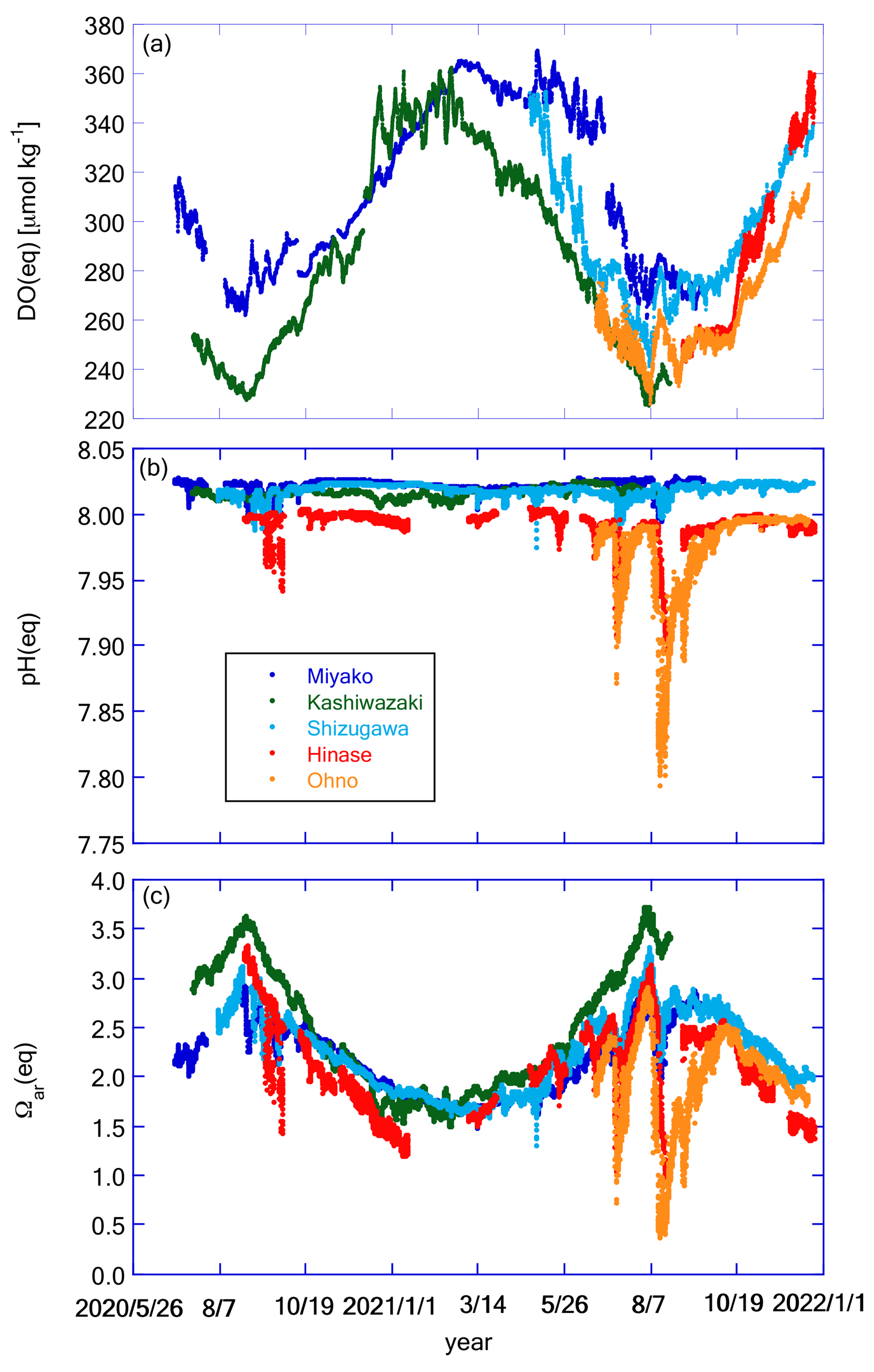
Figure 11Time series of (a) DO(eq), (b) pH(eq), and (c) Ωar(eq) at the five stations. Legends of color plots are the same for all panels as shown in (b).
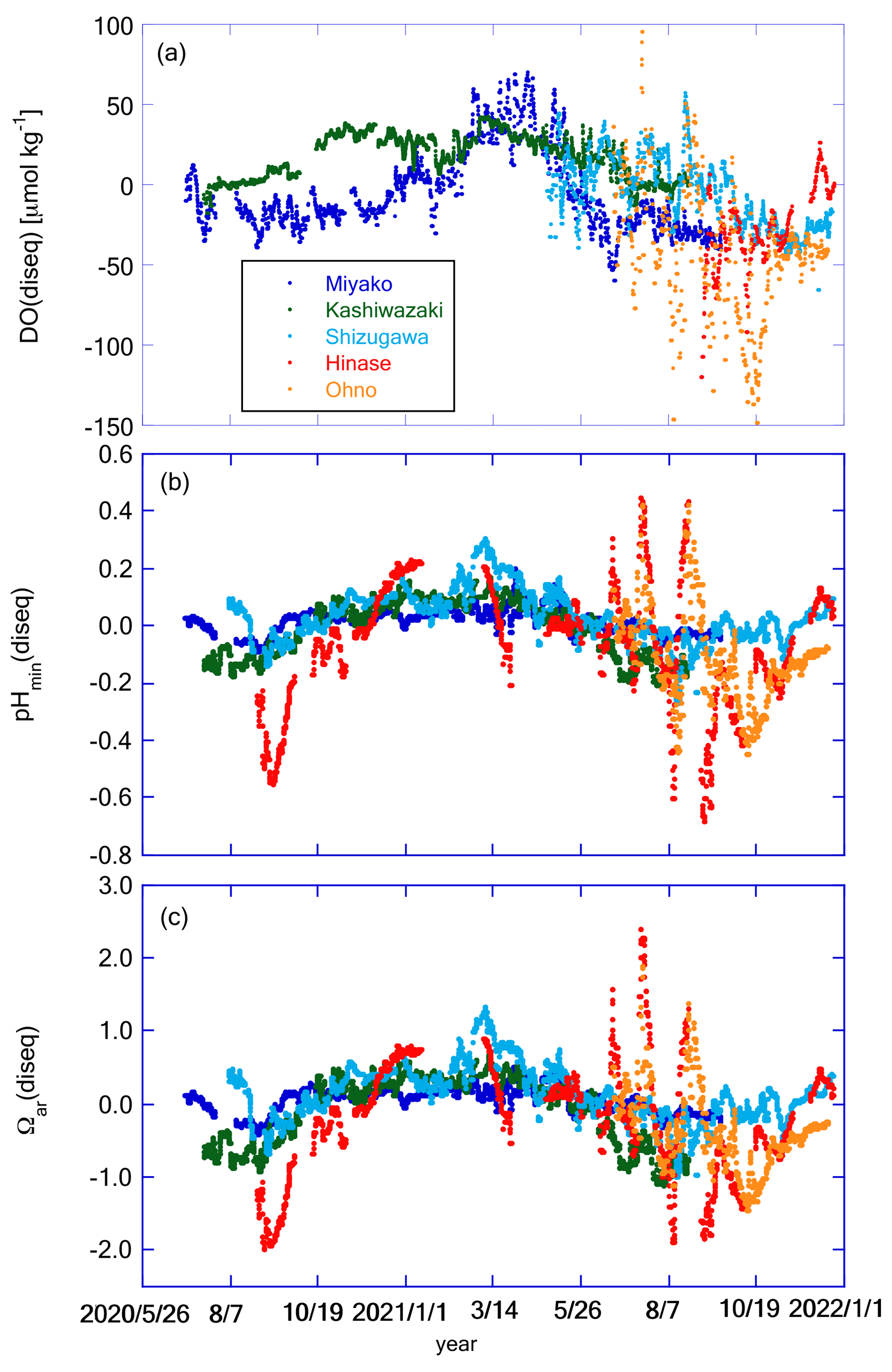
Figure 12Time series of (a) DO(diseq), (b) pHmin(diseq), and (c) Ωar(diseq) at the five stations. Legends of color plots are the same for all panels as shown in (a).
Figure 11 shows the temporal variation in DO(eq), pH(eq), and Ωar(eq), while Fig. 12 shows DO(diseq), pHmin(diseq), and Ωar(diseq). We also calculated 1-year SD, monthly SD, and 10 d SD for these parameters, and the results are listed in Table 4. The annual temporal variation was approximately the same between DO(eq) and DO(diseq) (Table 4), but their origin was significantly different. While seasonal variation played a dominant role in the temporal variation in DO(eq) (Fig. 11a; Table 4), short-term variations played a significant role in that of DO(diseq) (Fig. 12a; Table 4). In the case of pH, the temporal variation in pH(eq) resembles that of salinity (Figs. 7b and 11b), and the amplitude of pH(eq) (∼ 0.25; Fig. 11b) was approximately one order smaller than that of pH(diseq) (∼ 1.2; Fig. 12b). This result indicated that the thermodynamic process had a negligible contribution to the temporal variation in pH. Interestingly, the relative contributions of monthly SD and 10 d SD of pH(diseq) to the 1-year SD showed a similar structure to that of pHmin (Table 4), suggesting that the short-term variation at the scale of 10 d was the main driver of annual temporal variation for pHmin(diseq), which is similar to the cases of pHmin and salinity. Temporal variation in Ωar(eq) had both seasonal- and short-term scale components (Table 4), and the pattern of seasonal variation resembled that of water temperature, while that of short-term variation resembled that of salinity (Fig. 11c). Ωar(diseq) showed a similar scale of 1-year variability to that of Ωar(eq) (Figs. 11c and 12c; Table 4), similar to the case of DO. The temporal pattern of Ωar(diseq) was quite similar to that of pHmin(diseq), suggesting that short-term variation at the 10 d scale contributes significantly to the annual temporal variation in Ωar(diseq), similar to the case of pHmin(diseq). Overall, the non-thermodynamic component contributed approximately half of the observed annual variation in DO and Ωar, and in the case of pH, the non-thermodynamic component played a dominant role in the annual variation. For all these biogeochemical parameters, the short-term variation at the 10 d scale contributed a significant percentage of the temporal variation in the non-thermodynamic component.
Table 4Statistical features of thermodynamic and non-thermodynamic components.
To determine the specific process that drives the non-thermodynamic temporal variation in these properties, we examined the correlation between pHmin(diseq) and DO(diseq) (Fig. 13a). These two properties showed significant positive correlation, indicating that the non-thermodynamic component of temporal variations was driven mainly by biological processes. Several studies have also detected a positive relationship between variations in oxygen saturation and the metabolic component of pH in coastal waters, suggesting the primary influence of biological processes on pH dynamics (e.g., Baumann and Smith, 2018; Lowe et al., 2019). We further investigated the correlation between DICmax(diseq) and DO(diseq) (Fig. 13b); the former was calculated as pHmin(diseq) and Ωar(diseq). Most data obtained in Miyako and Ohno, and approximately 50 % of data obtained in Shizugawa, approximately followed a linear regression line with the slope of crossing the origin, suggesting that the observed temporal variations of both DICmax(diseq) and DO(diseq) were induced by the production or decomposition of planktonic oceanic particles with C:O2 ratio of 106 : 138 (Redfield et al., 1963) in these two areas. Such Redfield-type relationship between short-term variation in DO and that of DIC had also been observed in the coastal area of the East China Sea (Guo et al., 2021). The other data obtained in Shizugawa, as well as most data obtained in Hinase and Kashiwazaki, followed the regression lines with steeper slopes than that of open ocean stoichiometry.
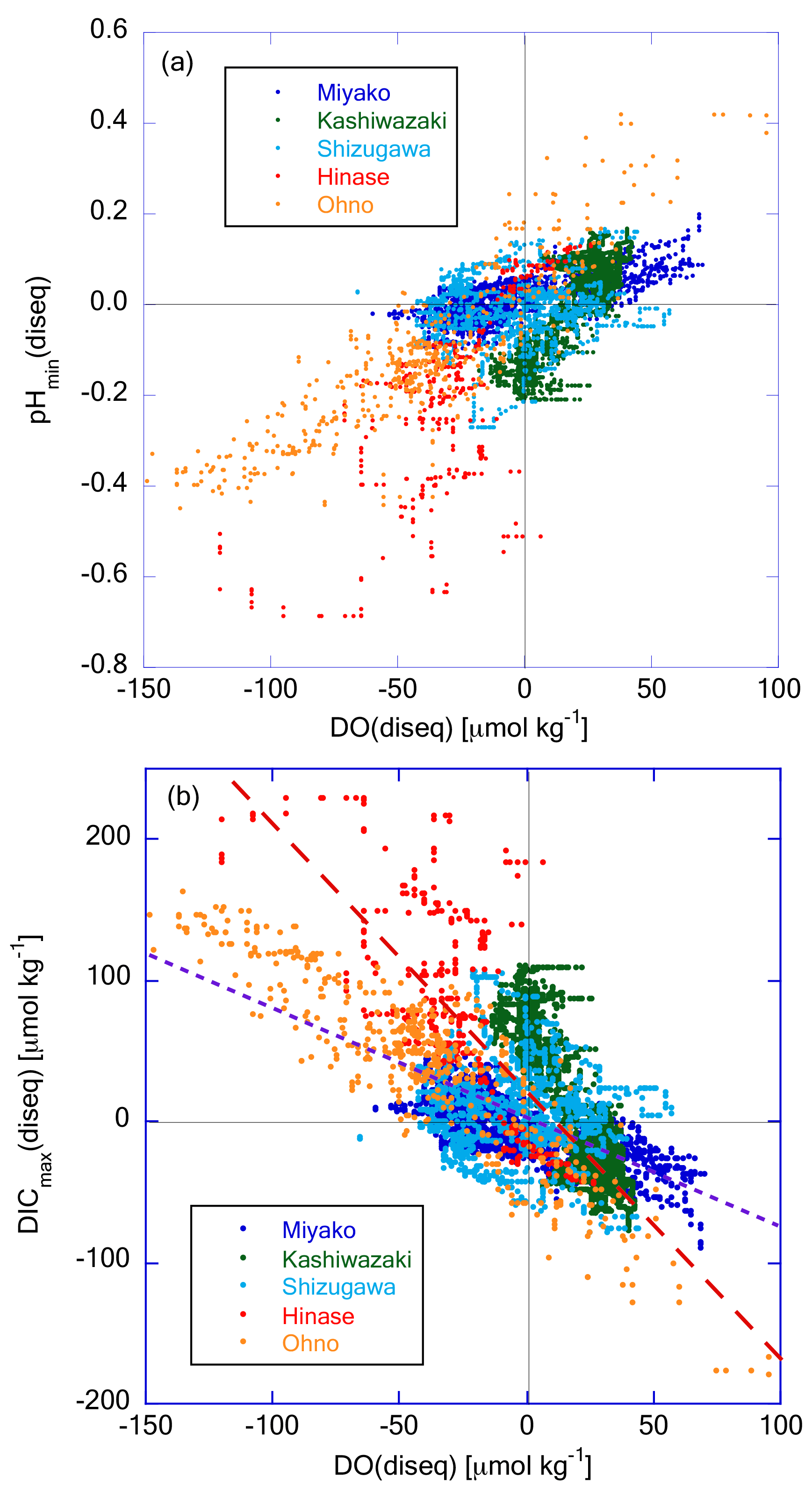
Figure 13Plot of (a) pHmin(diseq) and (b) DICmax(diseq) against DO(diseq), respectively. The dashed purple line in (b) represents the theoretical line when assuming that biological production or degradation of organic matter occurs with the Redfield relationship (). The dashed red line represents the regression line of Hinase data.
The respiratory quotients of estuarine ecosystems can occasionally be as high as 1.5 (Wang et al., 2018) or even 2.0 (Giblin et al., 1997), when affected by the anaerobic respiration process in estuarine sediments. The observed high ratio thus suggests that lateral propagation of biological processes in the neighboring estuaries contributes significantly to the observed temporal variations of DICmax(diseq) and DO(diseq) in these three areas. On the other hand, the turnover time of oxygen in ocean mixed layer due to air–sea gas exchange (in the range of several days to 2 weeks; Izett et al., 2018; Qin et al., 2021) is about 10 times shorter than that of CO2 (of the order of several months; e.g., Jones et al., 2014), reflecting their abundance in seawater. The ΔDO(diseq) that was once caused by biological processes therefore can recover to zero with shorter timescales than that of ΔDICmax(diseq) through the air–sea gas exchange process. The observed difference in ratio between Hinase and Ohno can also be explained by this mechanism, if large gas exchange processes (e.g., high wind speed and/or high wave height) have occurred in Hinase and not in Ohno. However, monthly-averaged wind speed was always higher in Ohno than in Hinase in the 2020 autumn (Japan Meteorological Agency weather record database; https://www.data.jma.go.jp/stats/etrn/index.php; last access: 5 January 2024), when low ΔDO(diseq) and high ΔDICmax(diseq) were mainly observed in this study (Fig. 12). Similarly, there is no significant difference in wind speed between two groups of Shizugawa data (one following Hinase data and the another following Ohno data). We thus conclude that relatively faster recovery of ΔDO(diseq) compared with that of ΔDICmax(diseq) through air–sea gas exchange is not the main cause of the observed high ratio, although this process may partly contribute to create a high ratio in these areas.
4.3 Controlling factor of the amplitude of short-term pH variation
Our analyses in Sects. 3.2 and 3.4 clearly show that severe low pH/low Ωar situations occur only at the short-term pH drawdown events that coincide with rainfall events in the coastal areas of Japan (Figs. 9c and 10c). As the amplitude of pH variation related to rainfall events differed among the five coastal areas, it is important to understand the controlling factor that determines the amplitude of short-term pH variation. To investigate this aspect, we analyzed the relationship of statistical short-term variabilities between salinity and pHmin. Since short-term variation mainly occurred on the timescale of <10 d for both salinity and pHmin (see discussion in Sect. 4.1), we plotted the avgSD of pHmin against that of salinity (Fig. 14). In this analysis, we introduced continuous monitoring data of pH and salinity obtained in Tokyo Bay (off Kawasaki artificial island; https://www.tbeic.go.jp/MonitoringPost/manual/aboutObservedPoint02.pdf; last access: 5 January 2024) to obtain information on highly eutrophic coastal areas. The details of the observation methods and the location settings of this station are described in Appendix B.
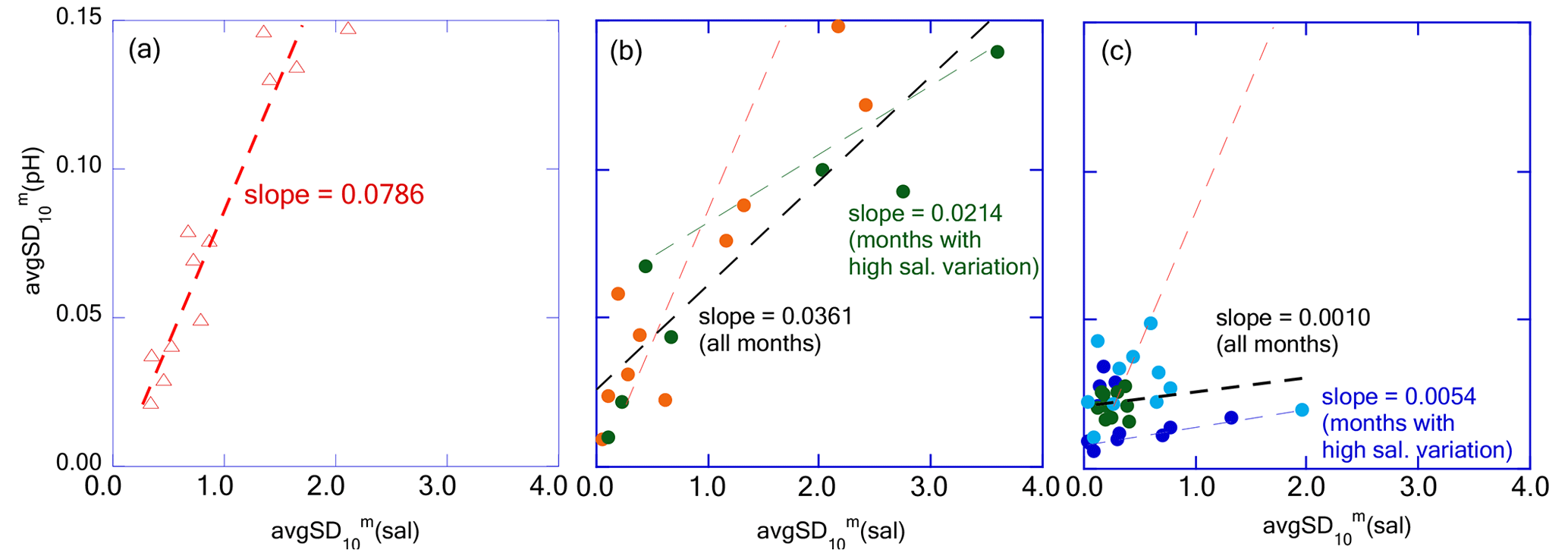
Figure 14Plots avgSD(pH) against avgSD(sal) for (a) Tokyo Bay, (b) Hinase and Ohno, and (c) Miyako, Kashiwazaki, and Shizugawa, respectively. The dashed red line represents the regression line of Tokyo Bay and the dashed black lines represent that of (b) Hinase and Ohno, and (c) Miyako, Kashiwazaki, and Shizugawa, respectively. Dashed green and blue lines represent regression lines of Hinase and Ohno, and Miyako, Kashiwazaki, and Shizugawa, respectively, with the data of months with the avgSD(sal) higher than 1.0.
In Tokyo Bay, the avgSD of pHmin (hereafter avgSD(pH)) linearly increased with an increase in avgSD of salinity (avgSD(sal); Fig. 14a), suggesting that freshwater transports the sources of biological processes (both organic carbon and dissolved nutrients) at a constant concentration regardless of the flow rate. On the other hand, in Hinase and Ohno, avgSD(pH) increased with that of avgSD(sal) at the same rate as observed in Tokyo Bay when avgSD(sal) was low but changed to a low value when avgSD(sal) exceeded 1.0 (Fig. 14b). Generally, suspended particle export of the river increases linearly with that of river discharge, while the percentage of particle organic materials (POM) within suspended particles decreases along with the increase in suspended particle export (e.g., Bukaveckas, 2022; Coynel et al., 2005; Point et al., 2007; Zhang et al., 2013). As a result, the increasing rate of the POM transport with that of river discharge tends to become weak when river discharge becomes high enough (Coynel et al., 2005; Kim et al., 2020). If we assume that short-term pH variation is mainly caused by the degradation of POM discharged from rivers into coastal areas and subsequential biological production by using nutrients released from the degraded POM (e.g., Kubo et al., 2017; Salisbury et al., 2008; Tokoro et al., 2020), we can expect that will also become small in the months with high river discharge (i.e., high avgSD(sal)). The observed result in this study also indicated that the concentration of biologically active materials transported by freshwater into the Seto Inland Sea was diluted at a high freshwater flow rate, while it was not diluted in the rivers flowing into Tokyo Bay, as the latter receives far higher anthropogenic nutrient loadings from its drainage basin than those received by the Seto Inland Sea. In the coastal area receiving further low anthropogenic nutrient loadings such as Miyako, Kashiwazaki, and Shizugawa, was much lower than that of Hinase and Ohno when (sal) exceeded 1.0 (Fig. 14c).
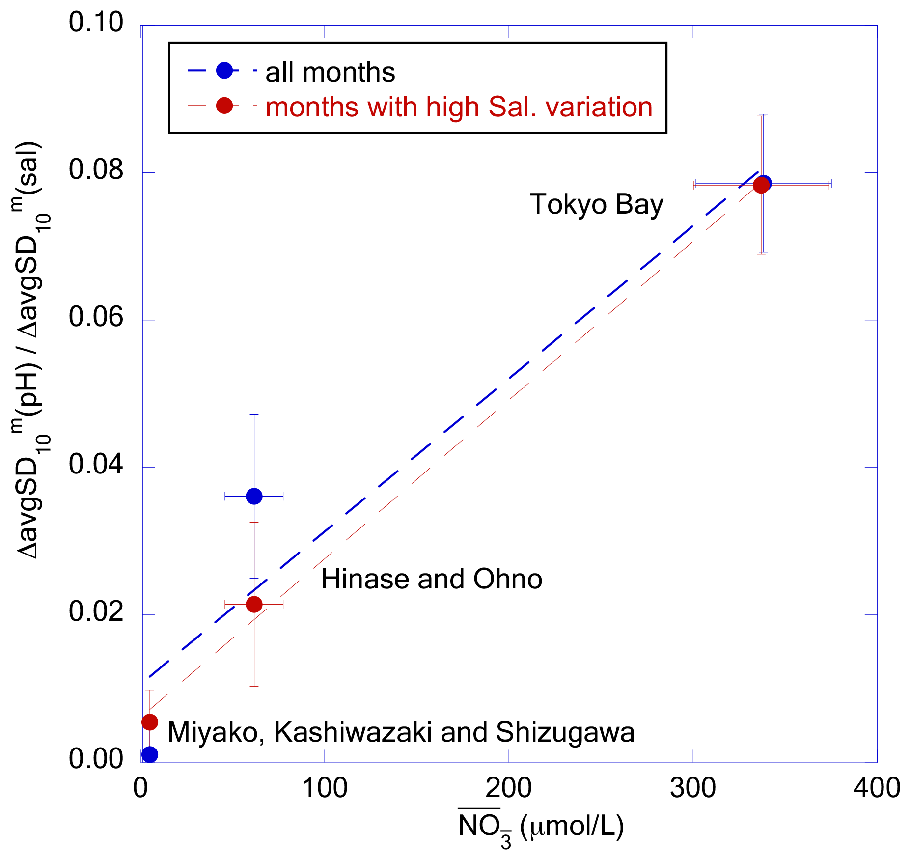
Figure 15Plot of against for each coastal area category. The blue and red dots represent the slope calculated from all months and from the months with avgSD(sal) higher than 1.0, respectively. The dashed lines represent the regression lines.
We determined the nutrient concentrations of the main freshwater sources for each of the three coastal area categories (i.e., respectively: Tashiro, Sabaishi, and Kitakami rivers for Miyako + Kashiwazaki + Shizugawa; Chikusa and Ohta rivers for Hinase + Ohno; and Ara, Tama, and Tsurumi rivers for Tokyo Bay) from the MOE Public Water Quality Database, and calculated the weighted mean nitrate concentration () of river waters that flow into each coastal area using water transport as the weight. We then found that observed at high freshwater input (that is, avgSD(sal) > 1.0) showed a linear relationship with in each coastal area category (Fig. 15). Even if we compare for all months, positive correlation against () was still significant. These results imply that the amplitude of short-term variation in pHmin in coastal areas is principally determined by the quantity of nutrients transported by freshwater from the hinterland. However, we note that the riverine nitrate concentration can be an implicit function of other controlling factors. For example, we recently observed that the quantity of suspended organic particles in river waters, as well as accumulated organic materials in riverine and estuarine sediments, are linearly correlated with the riverine nitrate concentration (Tsuneo Ono, unpublished data). Hence, the in Fig. 15 may actually be an indicator of the transport of these materials. We thus need further detailed observations, especially at the time of increase in water level of the river, to understand practical processes that cause short-term pH variation in coastal waters.
In this study, we synthesized data from continuous pH monitoring of five coastal areas in Japan from 2020 to 2021. Annual variability (∼ 1 SD) of pH and Ωar were 0.05–0.09 pH units and 0.25–0.29, respectively, for three areas with low anthropogenic nutrient loadings (Miyako Bay, Kashiwazaki Coast, and Shizugawa Bay), while they increased to 0.16–0.21 pH units and 0.52–0.58, respectively, in two areas with medium anthropogenic nutrient loadings (Hinase Archipelago and Ohno Strait in Seto Inland Sea). Statistical assessment of temporal variability at various timescales revealed that most of the annual variabilities in both pH and Ωar were controlled by short-term variation with a timescale of <10 d, rather than the seasonal-scale variation. Our analyses further illustrated that most of the short-term pH variation (and hence, annual variation) was caused by biological processes, while both thermodynamic and biological processes equally contributed to the temporal variation in Ωar. Biological alteration of pH mainly occurred in oceanic areas in Miyako Bay and Ohno Strait, whereas it occurred mainly in estuarine areas at Kashiwazaki Coast and Hinase Archipelago. In Shizugawa Bay, both oceanic and estuarine areas were responsible for the biological alteration of pH.
The observed results show that short-term acidification with Ωar of <1.5 occurred occasionally in Miyako and Shizugawa bays, while it occurred frequently in the Hinase Archipelago and Ohno Strait. Many such short-term acidification events were related to short-term low-salinity events. Our analyses showed that the amplitude of short-term pH variation was linearly correlated with that of short-term salinity variation, and its regression coefficient at the time of high freshwater input was positively correlated with the nutrient concentration of the main river that flows into the coastal area.
Fortunately, no marine organism that has been damaged by ocean acidification has been detected in coastal areas of Japan (Fujii et al., 2023). However, our study showed that Ωar in Japanese coastal areas occasionally drops to a level that is potentially hazardous for marine organisms, such as Pacific oysters (<1.5; Waldbusser et al., 2015), even in the present state. It is already known that the pH in Japanese coastal areas is decreasing at the same rate as that of the open ocean (Ishida et al., 2021; Ishizu et al., 2019), and hence, the extent, duration, and frequency of such short-term low pH and Ωar situations will increase in coastal areas in Japan in the future (Fujii et al., 2023). Our study indicates that the amplitude of the short-term drawdown of pH related to low-salinity events will decrease if we can reduce the nutrient concentration of rivers. Similar effects of anthropogenic nutrient reduction to diminish short-term Ωar drawdown in coastal waters are also reported by Kessouri et al. (2021). We note, however, that a certain percentage of Japanese coastal areas are now suffering due to the problem of low biological productivity derived from the decreased anthropogenic nutrient input (e.g., Yamamoto et al., 2021). We must consider the balance between the risk of ocean acidification and oligotrophication when we control anthropogenic loadings to coastal waters in the future. We also note that not only the concentration of dissolved nutrients, but also other biologically active materials, such as suspended organic materials in river waters and accumulated organic materials in riverine and estuarine sediments, may be responsible for short-term pH variations at low-salinity events (e.g., Carstensen and Duarte, 2019; Salisbury et al., 2008). Our analysis revealed that seawaters in both the Hinase Archipelago and Ohno Strait were oversaturated with CO2 all through the years, and hence, it is considered that more organic matter than that biologically produced within these areas was decomposed. In such cases, not only the reduction in dissolved nutrients but also the reduction in particulate organic matter transported from rivers to coastal areas will contribute to the suppression of short-term pH drawdown. Many studies have already mentioned the contribution of seaweed/seagrass beds to the effective capture of suspended organic sediments in estuaries (e.g., Barcelona et al., 2021; Leiva-Dueñas et al., 2023; Potouroglou et al., 2017), and hence, the conservation and/or development of seaweed/seagrass beds in estuarine and coastal areas will contribute to the reduction in organic matter transport from rivers to coastal areas at times of high river flow. To specify effective measures against the current coastal acidification in Japan, further detailed observations, especially at the time of increase in water level of the river, are needed such that we can obtain a detailed understanding of practical processes that cause short-term pH variation in coastal waters.
| SDa | annual standard deviation of each data |
| SDa〈m〉 | annual standard deviation of monthly average |
| SDm | monthly standard deviation of each data |
| avgSD | annual average of SDm |
| maxSD | annual maximum of SDm |
| SD10 | moving 10 d standard deviation of each data |
| avgSD | annual average of SD10 |
| maxSD | annual maximum of SD10 |
| avgSD | monthly average of SD10 |
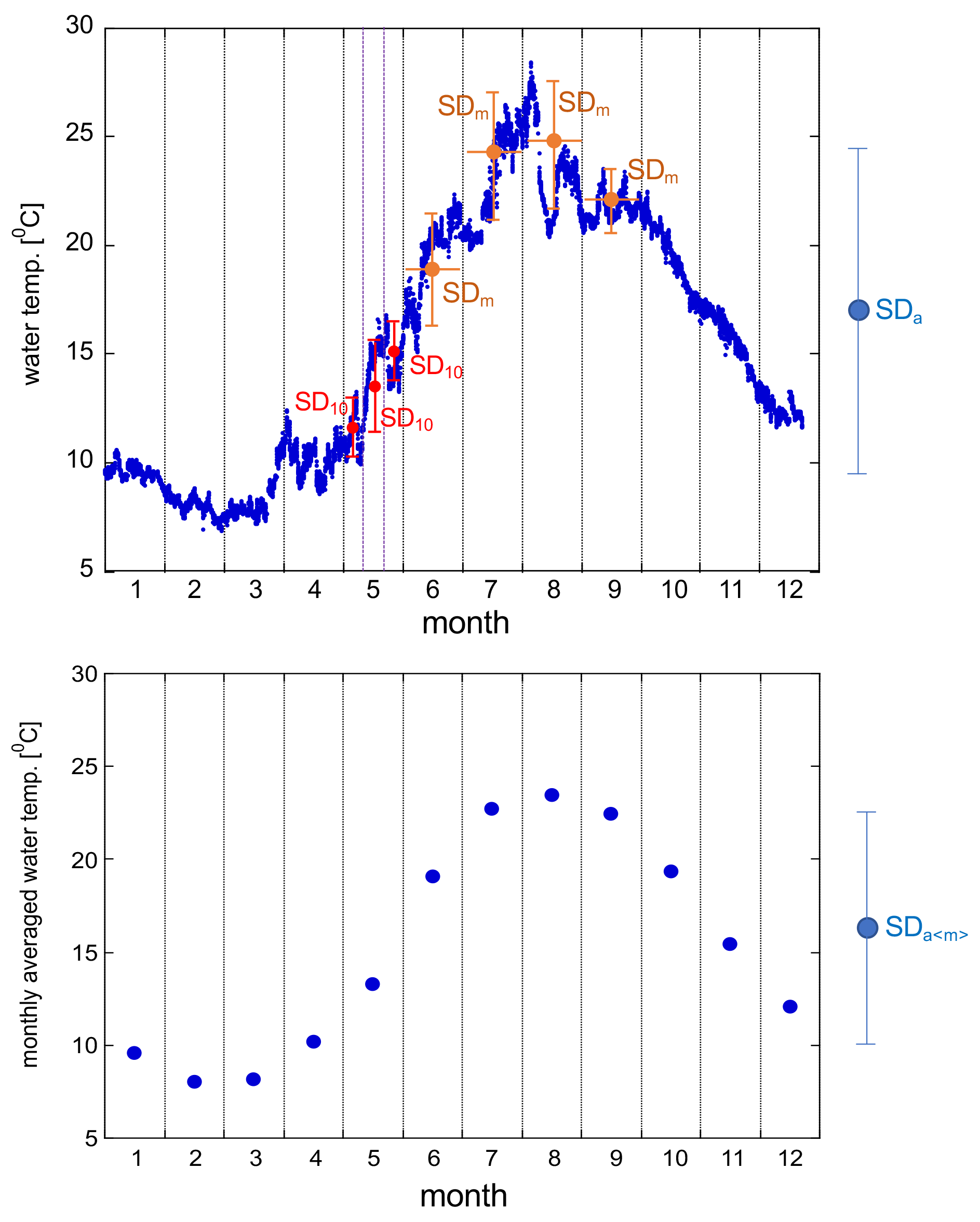
Figure A1Schematic diagram of statistical products SDa, SDa〈m〉, SDm, and SD10. While only three SD10s per month are presented in this diagram, we calculated each day's running SD10 by using ±5 d data to further calculate avgSD.
Detailed data for Tokyo Bay (Kawasaki artificial island; Sect. 4.3), referred to herein, are described by the data holders at https://www.tbeic.go.jp/MonitoringPost/manual/aboutObservedPoint02.pdf; (last access: 5 January 2024). Here, we provide a brief summary.
Kawasaki artificial island (KAI) is located in the center of Tokyo Bay, the bay with the highest population in its basin area (2.9 million) and highest nutrient loadings (210 tN d−1) in Japan. KAI is a huge concrete cylinder with a diameter of 200 m, in which an air vending system for the trans-bay freeway tunnel is stored. An autonomous ocean profiling system was set off KAI, which included a YSI 6600V2-4M multiple ocean sensor for the measurement of water temperature, salinity, and pH. The mechanical measurement resolution of the pH was ±0.01 pH units. The sensors were cleaned and calibrated on a monthly basis. Although the pH sensor was calibrated against NBS buffers, we used pH data without conversion to a total scale, as we used these pH data only for the analysis of temporal variability. Vertical profiles were measured hourly, and the obtained data were distributed from the public database managed by the Tokyo Bay Environmental Information Center (https://www.tbeic.go.jp/MonitoringPost/ViewGraph/ViewGraph?buoyId=02; last access: 5 January 2024). We downloaded KAI data pertaining to July 2020 to December 2021 from this database and used them for analysis.
Data from Tokyo Bay can be downloaded from the Tokyo Bay Environmental Information Center Public Database (https://www.tbeic.go.jp/MonitoringPost/ViewGraph/ViewGraph?buoyId=02, Tokyo Bay Environmental Information Center, 2024). Other data used in this study are provided in the Supplement.
The supplement related to this article is available online at: https://doi.org/10.5194/bg-21-177-2024-supplement.
TOn and DM performed field measurements and water sampling at Miyako Bay. MH and MY performed field measurements and water sampling at Kashiwazaki Coast. AD performed field measurements and water sampling at Shizugawa Bay. SO, TT, MF, and RH performed field measurements and water sampling at Hinase Archipelago. TOk, GO, and KS performed field measurements and water sampling at Ohno Strait. TOn undertook the measurements of discrete carbonate samples taken at Miyako Bay and Kashiwazaki Coast, and MW undertook the measurements of those taken at Shizugawa Bay, Hinase Archipelago, and Ohno Strait. Analyses of data obtained by these efforts were performed by TOn.
The contact author has declared that none of the authors has any competing interests.
Publisher’s note: Copernicus Publications remains neutral with regard to jurisdictional claims made in the text, published maps, institutional affiliations, or any other geographical representation in this paper. While Copernicus Publications makes every effort to include appropriate place names, the final responsibility lies with the authors.
We thank all fishers who helped us by providing their boats and support for monitoring at Shizugawa Bay and the Hinase Archipelago. We also thank Yukihiro Nojiri, Hideaki Nakata, Osamu Matsuda, Tetsuo Yanagi, and the reviewers of this paper for their fruitful advice and discussions during our analyses.
This research has been supported by the Environmental Restoration and Conservation Agency (grant no. JPMEERF20202007) and the Nippon Foundation (Ocean Acidification Adaptation Project).
This paper was edited by Koji Suzuki and reviewed by Abed El Rahman Hassoun and two anonymous referees.
Abo, K. and Onitsuka, G.: Characteristics of currents induced by heavy rainfall in Hiroshima Bay in July 2018, Proceedings of the Japan Society of Civil Engineers, Ser. B, 75, 1051–1056, 2019 (in Japanese).
Barcelona, A., Oldham, C., Colomer, J., Garcia-Orellana, J., and Serra, T.: Particle capture by seagrass canopies under an oscillatory flow, Coast. Eng., 169, 103972, https://doi.org/10.1016/j.coastaleng.2021.103972, 2021.
Barton, A., Hales, B., Waldbusser, G. G., Langdon, C., and Feely, R. A.: The Pacific oyster, Crassostrea gigas, shows negative correlation to naturally elevated carbon dioxide levels: Implications for near-term ocean acidification effects, Limnol. Oceanogr., 57, 698–710, https://doi.org/10.4319/lo.2012.57.3.0698, 2012.
Bates, N. R., Astor, Y. M., Church, M. J., Currie, K., Dore, J. E., González-Dávila, M., Lorenzoni, L., Muller-Karger, F., Olafsson, J., and Santana-Casiano, J. M.: A time-series view of changing surface ocean chemistry due to ocean uptake of anthropogenic CO2 and ocean acidification, Oceanography, 27, 126–141, https://doi.org/10.5670/oceanog.2014.16, 2014.
Baumann, H. and Smith, E. M.: Quantifying metabolically driven pH and oxygen fluctuations in US nearshore habitats at diel to interannual timescales, Estuar. Coast., 41, 1102–1117, https://doi.org/10.1007/s12237-017-0321-3, 2018.
Bednaršek, N., Beck, M. W., Pelletier, G., Applebaum, S. L., Feely, R. A., Butler, R., Byrne, M., Peabody, B., Davis, J., and Štrus, J.: Natural analogues in pH variability and predictability across the Coastal Pacific estuaries: extrapolation of the increased oyster dissolution under increased pH amplitude and low predictability related to ocean acidification, Environ. Sci. Technol., 56, 9015–9028, https://doi.org/10.1021/acs.est.2c00010, 2022.
Bernardo, L. P. C., Fujii, M., and Ono, T.: Development of a high-resolution marine ecosystem model for predicting the combined impacts of ocean acidification and hypoxia, Front. Mar. Sci., 10, 1174892, https://doi.org/10.3389/fmars.2023.1174892, 2023.
Booth, J. A. T., McPhee-Shaw, E. E., Chua, P., Kingsley, E., Denny, M., Phillips, R., Bograd, S. J., Zeidberg, L. D., and Gilly, W. F.: Natural intrusions of hypoxic, low pH water into nearshore marine environments on the California coast, Cont. Shelf Res., 45, 108–115, https://doi.org/10.1016/j.csr.2012.06.009, 2012.
Borges, A. V. and Gypens, N.: Carbonate chemistry in the coastal zone responds more strongly to eutrophication than to ocean acidification, Limnol. Oceanogr., 55, 346–353, 2010.
Borges, A. V., Delille, B., and Frankignoulle, M.: Budgeting sinks and sources of CO2 in the coastal ocean: Diversity of ecosystems counts, Geophys. Res. Lett., 32, L14601, https://doi.org/10.1029/2005GL023053, 2005.
Bukaveckas, P. A.: Carbon dynamics at the river–estuarine transition: a comparison among tributaries of Chesapeake Bay, Biogeosciences, 19, 4209–4226, https://doi.org/10.5194/bg-19-4209-2022, 2022.
Cai, W.-J., Hu, X., Huang, W.-J., Murrell, M. C., Lehrter, J. C., Lohrenz, S. E., Chou, W.-C., Zhai, W., Hollibaugh, J. T., Wang, Y., Zhao, P., Guo, X., Gundersen, K., Dai, M., and Gong, G.-C.: Acidification of subsurface coastal waters enhanced by eutrophication, Nat. Geosci., 4, 1297, https://doi.org/10.1038/ngeo1297, 2011.
Cai, W.-J., Huang, W.-J., Luther III, G. W., Pierrot, D., Li, M., Testa, J., Xue, M., Joesoef, A., Mann, R., Brodeur, J., Xu, Y.-Y., Chen, B., Waldbusser, G. G., Cornwell, J., and Kemp, W. M.: Redox reactions and weak buffering capacity lead to acidification in the Chesapeake Bay, Nat. Commun., 8, 369, https://doi.org/10.1038/s41467-017-00417-7, 2017.
Carstensen, J. and Duarte, C. M.: Drivers of pH variability in coastal ecosystems, Environ. Sci. Technol., 53, 4020–4029, https://doi.org/10.1021/acs.est.8b03655, 2019.
Christian, J. and Ono, T.: Ocean acidification and deoxygenation in the North Pacific Ocean, North Pacific Marine Science Organization, Sidney, 116 pp., ISBN 978-1-927797-32-7, 2019.
Coynel, A., Seyler, P., Etcheber, H., Meybeck, M., and Orange, D.: Spatial and seasonal dynamics of total suspended sediment and organic carbon species in the Congo River, Global Biogeochem. Cy., 19, GB4019, https://doi.org/10.1029/2004GB002335, 2005.
Delille, B., Borges, A. V., and Delille, D.: Influence of giant kelp beds (Macrocystis pyrifera) on diel cycles of pCO2 and DIC in the Sub-Antarctic coastal area, Estuar. Coast. Shelf S., 81, 114–122, https://doi.org/10.1016/j.ecss.2008.10.004, 2009.
Dickson, A. G.: Standard potential of the reaction: AgCl(s) + 12H2(g) = Ag(s) + HCl(aq), and the standard acidity constant of the ion HSO in synthetic sea water from 273.15 to 318.15 K, J. Chem. Thermodyn., 22, 113–127, https://doi.org/10.1016/0021-9614(90)90074-Z, 1990.
Duarte, C. M., Hendriks, I. E., Moore, T. S., Olsen, Y. S., Steckbauer, A., Ramajo, L., Carstensen, J., Trotter, J. A., and McCulloch, M.: Is ocean acidification an open-ocean syndrome? Understanding anthropogenic impacts on seawater pH, Estuar. Coast., 36, 221–236, https://doi.org/10.1007/s12237-013-9594-3, 2013.
Feely, R. A., Sabine, C. L., Hernandez-Ayon, J. M., Ianson, D., and Hales, B.: Evidence for upwelling of corrosive “acidified” water onto the continental shelf, Science, 320, 1490e1492, https://doi.org/10.1126/science.1155676, 2008.
Feely, R. A., Alin, S. R., Carter, B., Bednarsek, N., Hales, B., Chan, F., Hill, T. M., Gaylord, B., Sanford, E., Byrne, R. H., Sabine, C. L., Greeley, D., and Juranek, L.: Chemical and biological impacts of ocean acidification along the west coast of North America, Estuar. Coast. Shelf S., 183, 260–270, https://doi.org/10.1016/j.ecss.2016.08.043, 2016.
Frieder, C. A., Nam, S. H., Martz, T. R., and Levin, L. A.: High temporal and spatial variability of dissolved oxygen and pH in a nearshore California kelp forest, Biogeosciences, 9, 3917–3930, https://doi.org/10.5194/bg-9-3917-2012, 2012.
Fujii, M., Takao, S., Yamaka, T., Akamatsu, T., Fujita, Y., Wakita, M., Yamamoto, A., and Ono, T.: Continuous monitoring and future projection of ocean warming, acidification, and deoxygenation on the subarctic coast of Hokkaido, Japan, Front. Mar. Sci., 8, 590020, https://doi.org/10.3389/fmars.2021.590020, 2021.
Fujii, M., Hamanoue, R., Bernardo, L. P. C., Ono, T., Dazai, A., Oomoto, S., Wakita, M., and Tanaka, T.: Assessing impacts of coastal warming, acidification, and deoxygenation on Pacific oyster (Crassostrea gigas) farming: a case study in the Hinase area, Okayama Prefecture, and Shizugawa Bay, Miyagi Prefecture, Japan, Biogeosciences, 20, 4527–4549, https://doi.org/10.5194/bg-20-4527-2023, 2023.
Giblin, A. E., Hopkinson, C. S., and Tucker, J.: Benthic metabolism and nutrient cycling in Boston Harbor, Mountains, Estuaries, 20, 346–364, https://doi.org/10.2307/1352349, 1997.
Gomez, F. A., Wanninkhof, R., Barbero, L., and Lee, S.-K.: Increasing river alkalinity slows ocean acidification in the northern Gulf of Mexico, Geophys. Res. Lett., 48, e2021GL096521, https://doi.org/10.1029/2021GL096521, 2021.
Guo, X., Yao, Z., Gao, Y., Luo, Y., Xu, Y., and Zhai, W.: Seasonal variability and future projection of ocean acidification on the East China Sea shelf off the Changjiang Estuary, Front. Mar. Sci., 8, 770034, https://doi.org/10.3389/fmars.2021.770034, 2021.
Hauri, C., Gruber, N., Vogt, M., Doney, S. C., Feely, R. A., Lachkar, Z., Leinweber, A., McDonnell, A. M. P., Munnich, M., and Plattner, G.-K.: Spatiotemporal variability and long-term trends of ocean acidification in the California Current System, Biogeosciences, 10, 193–216, https://doi.org/10.5194/bg-10-193-2013, 2013.
Higashi, H., Sato, Y., Yoshinari, H., Maki, H., Koshikawa, H., Kanaya, G., and Uchiyama, Y.: Freshwater discharge from small river basins and its impacts on reproductivity of coastal hydrodynamic simulation in Seto Inland Sea, Proceedings of the Japan Society of Civil Engineers, Ser. B, 74, 1135–11140, 2018 (in Japanese).
Hofmann, G. E., Smith, J. E., Johnson, K. S., Send, U., Levin, L. A., Micheli, F., Paytan, A., Price, N. N., Peterson, B., Takeshita, Y., Matson, P. G., Crook, E. D., Kroeker, K. J., Gambi, M. C., Rivest, E. B., Frieder, C. A., Yu, P. C., and Martz, T. R.: High-Frequency Dynamics of Ocean pH: A Multi-Ecosystem Comparison, Plos One, 6, e28983, https://doi.org/10.1371/journal.pone.0028983, 2012.
Hoshiba, Y., Hasumi, H., Itoh, S., Matsumura, Y., and Nakada, S.: Biogeochemical impacts of flooding discharge with high suspended sediment on coastal seas: A modelling study for a microtidal open bay, Sci. Rep.-UK, 11, 21322, https://doi.org/10.1038/s41598-021-00633-8, 2021.
Iida, Y., Takatani, Y., Kojima, A., and Ishii, M.: Global trends of ocean CO2 sink and ocean acidification: an observation-based reconstruction of surface ocean inorganic carbon variables, J. Oceanogr., 77, 323–358, https://doi.org/10.1007/s10872-020-00571-5, 2021.
Ishida, H., Isono, R. S., Kita, J., and Watanabe, Y. W.: Long-term ocean acidification trends in coastal waters around Japan, Nat. Sci. Rep., 11, 5052, https://doi.org/10.1038/s41598-021-84657-0, 2021.
Ishizu, M., Miyazawa, Y., Tsunoda, T., and Ono, T.: Long-term trends in pH in Japanese coastal seawater, Biogeosciences, 16, 4747–4763, https://doi.org/10.5194/bg-16-4747-2019, 2019.
Izett, R. W., Manning, C. C., Hamme, R. C., and Tortell, P. D.: Refined estimates of net community production in the Subarctic Northeast Pacific derived from measurements with N2O-based corrections for vertical mixing, Global Biogeochem. Cy., 32, 326–350, https://doi.org/10.1002/2017GB005792, 2018.
JFA (Japan Fisheries Agency): Final report of the research for forest – river – ocean linkage for the creation of appropriate fisheries environment, Japan Fisheries Agency, 118 pp., https://www.jfa.maff.go.jp/j/gyoko_gyozyo/pdf/sub70a.pdf (last access: 5 January 2024), 2004 (in Japanese).
Jiang, L.-Q., Carter, B. R., Feely, R. A., Lauvset, S. K., and Olsen, A.: Surface ocean pH and buffer capacity: past, present and future, Nat. Sci. Rep., 9, 18624, https://doi.org/10.1038/s41598-019-55039-4, 2019.
Jiang, Z.-P., Tyrrell, T., Hydes, D. J., Dai, M., and Hartman, S. E.: Variability of alkalinity and the alkalinity-salinity relationship in the tropical and subtropical surface ocean, Glob. Biogeochem. Cy., 28, 729–742, https://doi.org/10.1002/2013GB004678, 2014.
Johnson, Z. I., Wheeler, B. J., Blinebry, S. K., Carlson, C. M., Ward, C. S., and Hunt, D. E.: Dramatic variability of the carbonate system at a temperate coastal ocean site (Beaufort, North Carolina, USA) is regulated by physical and biogeochemical processes on multiple timescales, PLoS ONE, 8, e85117, https://doi.org/10.1371/journal.pone.0085117, 2013.
Jones, D. C., Ito, T., Takano, Y., and Hsu, W.-C.: Spatial and seasonal variability of the air-sea equilibration timescale of carbon dioxide, Global Biogeochem. Cy., 28, 1163–1178, https://doi.org/10.1002/2014GB004813, 2014.
Kakehi, S., Naiki, K., Kodama, T., Wagawa, T., Kuroda, H., and Ito, S.-I.: Projections of nutrient supply to a wakame (Undaria pinnatifida) seaweed farm on the Sanriku Coast of Japan, Fish. Oceanogr., 27, 323–335, https://doi.org/10.1111/fog.12255, 2018.
Kessouri, F., McWilliams, J. C., Bianchi, D., Sutula, M., Renault, L., Deutsch, C., Feely, R. A., McLaughlin, K., Ho, M., Howard, E. M., Bednaršek, N., Damien, P., Molemaker, J., and Weisberg, S. B.: Coastal eutrophication drives acidification, oxygen loss, and ecosystem change in a major oceanic upwelling system, P. Natl. Acad. Sci. USA, 118, e2018856118, https://doi.org/10.1073/pnas.2018856118, 2021.
Kim, J., Blair, N. E., Ward, A. S., and Goff, K.: Storm-induced dynamics of particulate organic carbon in Clear Creek, Iowa: An intensively managed landscape critical zone observatory story, Front. Water, 2, 578261, https://doi.org/10.3389/frwa.2020.578261, 2020.
Ko, Y. H., Lee, K., Noh, J. H., Lee, C. M., Kleypas, J. A., Jeong, H. J., and Kim, K. Y.: Influence of ambient water intrusion on coral reef acidification in the Chuuk Lagoon, located in the coral-rich western Pacific Ocean, Geophys. Res. Lett., 43, 3830–3838, https://doi.org/10.1002/2016GL068234, 2016.
Kobayashi, J.: Study on average water quality of Japanese rivers and its features, Studies in Agriculture, 48, 63–104, 1960 (in Japanese).
Kubo, A., Maeda, Y., and Kanda, J.: A significant net sink for CO2 in Tokyo Bay, Nat. Sci. Rep., 7, 44355, https://doi.org/10.1038/srep44355, 2017.
Kurihara, H., Kato, S., and Ishimatsu, A.: Effects of increased seawater pCO2 on early development of the oyster Crassostrea gigas, Aquat. Biol., 1, 91–98, 2007.
Laruelle, G. G., Dürr, H. H., Slomp, C. P., and Borges, A. V.: Evaluation of sinks and sources of CO2 in the global coastal ocean using a spatially explicit typology of estuaries and continental shelves, Geophys. Res. Lett., 37, L15607, https://doi.org/10.1029/2010GL043691, 2010.
Lauvset, S. K., Gruber, N., Landschützer, P., Olsen, A., and Tjiputra, J.: Trends and drivers in global surface ocean pH over the past 3 decades, Biogeosciences, 12, 1285–1298, https://doi.org/10.5194/bg-12-1285-2015, 2015.
Lee, K., Kim, T.-W., Bryne, R. H., Millero, F. J., Feely, R. A., and Liu, Y.-M.: The universal ratio of boron to chlorinity for the North Pacific and North Atlantic oceans, Geochim. Cosmochim. Ac., 74, 1801–1811, https://doi.org/10.1016/j.gca.2009.12.027, 2010.
Leiva-Dueñas, C., Graversen, A. E. L., Banta, G. T., Holmer, M., Masque, P., Stæhr, P. A. U., and Krause-Jensen, D.: Capturing of organic carbon and nitrogen in eelgrass sediments of southern Scandinavia, Limnol. Oceanogr., 68, 631–648, https://doi.org/10.1002/lno.12299, 2023.
Lowe, A. T., Bos, J., and Ruesink, J.: Ecosystem metabolism drives pH variability and modulates long-term ocean acidification in the Northeast Pacific coastal ocean, Nat. Sci. Rep., 9, 963, https://doi.org/10.1038/s41598-018-37764-4, 2019.
Lueker, T. J., Dickson, A. G., and Keeling, C. D.: Ocean pCO2 calculated from dissolved inorganic carbon, alkalinity, and equations for K1 and K2: validation based on laboratory measurements of CO2 in gas and seawater at equilibrium, Mar. Chem., 70, 105–119, https://doi.org/10.1016/S0304-4203(00)00022-0, 2000.
MOE (Ministry of Environment, Japan): Public Water Quality Database, https://water-pub.env.go.jp/water-pub/mizu-site/mizu/kousui/dataMap.asp (last access: 29 October 2022), 2022.
Mongin, M., Baird, M. E., Tilbrook, B., Matear, R. J., Lenton, A., Herzfeld, M., Wild-Allen, K., Skerratt, J., Margvelashvili, N., Robson, B. J., Duarte, C. M., Gustafsson, M. S. M., Ralph, P. J., and Steven, A. D. L.: The exposure of the Great Barrier Reef to ocean acidification, Nat. Commun., 7, 10732, https://doi.org/10.1038/ncomms10732, 2016.
Niigata Prefectural Institution of Fisheries Oceanography: 1997 Annual report of ocean monitoring for ocean climate forecast for fisheries, Niigata Prefectural Institution of Fisheries Oceanography, NCID: AA11237561, 106 pp., 1998 (in Japanese).
Nishijima, W.: Management of nutrient concentrations in the Seto Inland Sea, Bulletin on Coastal Oceanography, 56, 13–19, 2018 (in Japanese).
Okada, T., Maruya, Y., Nakayama, K., and Iseri, E.: A study on restoration of eelgrass (Zostera marina) damaged by tsunami in Miyako Bay, Proceedings of the Japan Society of Civil Engineers, Ser. B, 70, 1186–1190, 2014 (in Japanese).
Onitsuka, T., Takami, H., Muraoka, D., Matsumoto, Y., Nakatsubo, A., Kimura, R., Ono, T., and Nojiri, Y.: Effects of ocean acidification with pCO2 diurnal fluctuations on survival and larval shell formation of Ezo abalone, Haliotis discus hannai, Mar. Environ. Res., 134, 28–36, https://doi.org/10.1016/j.marenvres.2017.12.015, 2018.
Papalexiou, S. M. and Montanari, A.: Global and regional increase of precipitation extremes under global warming, Water Resour. Res., 55, 4901–4914, https://doi.org/10.1029/2018WR024067, 2019.
Pierrot, D., Lewis, E., and Wallace, D. W. R.: MS Excel Program Developed for CO2 System Calculations, ORNL/CDIAC-105a, Carbon Dioxide Information Analysis Center, Oak Ridge National Laboratory, U.S. Department of Energy, Oak Ridge, Tennessee, 2006.
Point, D., Bareille, G., Amouroux, D., Etcheber, H., and Donard, O. F. X.: Reactivity, interactions and transport of trace elements, organic carbon and particulate material in a mountain range river system (Adour River, France), J. Environ. Monitor., 9, 157–167, https://doi.org/10.1039/b616312b, 2007.
Potouroglou, M., Bull, J. C., Krauss, K. W., Kennedy, H. A., Fusi, M., Daffonchio, D., Mangora, M. M., Githaiga, M. N., Diele, K., and Huxham, M.: Measuring the role of seagrasses in regulating sediment surface elevation, Nat. Sci. Rep., 7, 11917, https://doi.org/10.1038/s41598-017-12354-y, 2017.
Provoost, P., van Heuven, S., Soetaert, K., Laane, R. W. P. M., and Middelburg, J. J.: Seasonal and long-term changes in pH in the Dutch coastal zone, Biogeosciences, 7, 3869–3878, https://doi.org/10.5194/bg-7-3869-2010, 2010.
Qin, C., Zhang, G., Zheng, W., Han, Y., and Liu, S.: High-resolution distributions of on the northern slope of the South China Sea and estimates of net community production, Ocean Sci., 17, 249–264, https://doi.org/10.5194/os-17-249-2021, 2021.
Redfield, A. C., Ketchum, B. H., and Richards, F. A.: The influence of organisms on the composition of sea-water, The Sea, Vol. 2, edited by: Hill, M. N., 26–77, Interscience, New York, ISBN 9780674017283, 1963.
Ricart, A. M., Ward, M., Hill, T. M., Sanford, E., Kroeker, K. J., Takeshita, Y., Merolla, S., Shukla, P., Ninokawa, A. T., Elsmore, K., and Gaylord, B.: Coast-wide evidence of low pH amelioration by seagrass ecosystems, Glob. Change Biol., 27, 2580–2591, https://doi.org/10.1111/gcb.15594, 2021.
Rosenau, N. A., Galavotti, H., Yates, K. K., Bohlen, C. C., Hunt, C. W., Liebman, M., Brown, C. A., Pacella, S. R., Largier, J. L., Nielsen, K. J., Hu, X., McCutcheon, M. R., Vasslides, J. M., Poach, M., Ford, T., Johnston, K., and Steele, A.: Integrating High-resolution coastal acidification monitoring data across seven United States Estuaries, Front. Mar. Sci., 8, 679913, https://doi.org/10.3389/fmars.2021.679913, 2021.
Salisbury, J., Green, M., Hunt, C., and Campbell, J.: Coastal acidification by rivers: A threat to shellfish?, EOS, 89, 513–528, https://doi.org/10.1029/2008EO500001, 2008.
Salisbury, J. E. and Jönsson, B. F.: Rapid warming and salinity changes in the Gulf of Maine alter surface ocean carbonate parameters and hide ocean acidification, Biogeochemistry, 141, 401–418, https://doi.org/10.1007/s10533-018-0505-3, 2018.
Sugimura, A., Takeda, A., Nihei, Y., and Ohtsuki, K.: Evaluation of sediment, nutrient and organic matter transport from a wide range of land to coastal ocean, Proceedings of the Japan Society of Civil Engineers, Ser. B, 71, 1423–1428, 2015 (in Japanese).
Sunda, W. G. and Cai, W.-J.: Eutrophication induced CO2-acidification of subsurface coastal waters: Interactive effects of temperature, salinity, and atmospheric pCO2, Environ. Sci. Technol., 46, 10651–10659, https://doi.org/10.1021/es300626f, 2012.
Takahashi, T., Sutherland, S. C., Chipman, D. W., Goddard, J. G., Ho, C., Newberger, T., Sweeney, C., and Munro, D. R.: Climatological distributions of pH, pCO2, total CO2, alkalinity, and CaCO3 saturation in the global surface ocean, and temporal changes at selected locations, Mar. Chem., 164, 95–125, https://doi.org/10.1016/j.marchem.2014.06.004, 2014.
Takatani, Y., Enyo, K., Iida, Y., Kojima, A., Nakano, T., Sasano, D., Kosugi, N., Midorikawa, T., Suzuki, T., and Ishii, M.: Relationships between total alkalinity in surface water and sea surface dynamic height in the Pacific Ocean, J. Geophys. Res., 119, 2806–2814, https://doi.org/10.1002/2013JC009739, 2014.
Tokoro, T., Nakaoka, S.-O., Takao, S., Kuwae, T., Kubo, A., Endo, T., and Nojiri, Y.: Contribution of biological effects to carbonate system variations and the air–water CO2 flux in urbanised bays in Japan, J. Geophys. Res., 126, e2020JC016974, https://doi.org/10.1029/2020JC016974, 2020.
Tokyo Bay Environmental Information Center: Continuous monitoring data for the water quality of Tokyo Bay, Tokyo Bay Environmental Information Center [data set], https://www.tbeic.go.jp/MonitoringPost/ViewGraph/ViewGraph?buoyId=02, last access: 5 January 2024.
Tsukamoto, H. and Yanagi, T.: Temporal and Spatial variations in water temperature, salinity, pH, nutrient salts and chlorophill-a in the Seto Inland Sea, Umi no Kenkyu, 7, 11–19, 1998 (in Japanese).
Vargas, C. A., Contreras, P. Y., Pérez, C. A., Sobarzo, M., Saldías, G. S., and Salisbury, J.: Influences of riverine and upwelling waters on the coastal carbonate system off Central Chile and their ocean acidification implications, J. Geophys. Res., 121, 1468–1483, https://doi.org/10.1002/2015JG003213, 2015.
Venkatesan, R., Senthilkumar, P., Vedachalam, N., and Murugesh, P.: Biofouling and its effects in sensor mounted moored observatory system in Northern Indian Ocean, Int. Biodeterior. Biodegr., 116, 198–204, https://doi.org/10.1016/j.ibiod.2016.10.034, 2017.
Wakita, M., Sasaki, K., Nagano, A., Abe, H., Tanaka, T., Nagano, K., Sugie, K., Kaneko, H., Kimoto, K., Okunishi, T., Takada, M., Yoshino, J., and Watanabe, S.: Rapid reduction of pH and CaCO3 saturation state in the Tsugaru Strait by the intensified Tsugaru Warm Current during 2012–2019, Geophys. Res. Lett., 48, e2020GL091332, https://doi.org/10.1029/2020GL091332, 2021.
Waldbusser, G. G. and Salisbury, J. E.: Ocean acidification in the coastal zone from an organism's perspective: Multiple system parameters, frequency domains, and habitats, Annu. Rev. Mar. Sci., 6, 221–247, https://doi.org/10.1146/annurev-marine-121211-172238, 2014.
Waldbusser, G. G., Hales, B., Langdon, C. J., Haley, B. A., Schrader, P., Brunner, E. L., Gray, M. W., Miller, C. A., and Gimenez, I.: Saturation-state sensitivity of marine bivalve larvae to ocean acidification, Nat. Clim. Change, 5, 273–280, https://doi.org/10.1038/NCLIMATE2479, 2015.
Wallace, R. B., Baumann, H., Grear, J. S., Aller, R. C., and Gobler, C. J.: Coastal ocean acidification: The other eutrophication problem, Estuar. Coast. Shelf Sc., 148, 1–13, https://doi.org/10.1016/j.ecss.2014.05.027, 2014.
Wang, S. R., Iorio, D. D., Cai, W.-J., and Hopkinson, C. S.: Inorganic carbon and oxygen dynamics in a marsh-dominated estuary, Limnol. Oceanogr., 63, 47–71, https://doi.org/10.1002/lno.10614, 2018.
WDCGG (World Data Centre for Greenhouse Gases): Current State of GHCs, https://gaw.kishou.go.jp/publications/global_mean_mole_fractions, last access: 5 January 2024.
Weiss, R. F.: The solubility of nitrogen, oxygen and argon in water and seawater, Deep-Sea Res., 17, 721–735, 1970.
Yamamoto, H., Yoshiki, K., Komatsu, T., Sasa, S., Hayama, M., Murata, H., and Yanagi, T.: Numerical evaluation of environmental capacity of aquaculture in Shizugawa Bay – comparison before and after the Great East Japan Earthquake, Proceedings of the Japan Society of Civil Engineers, Ser. B, 73, 1339–1344, 2017.
Yamamoto, H., Yoshiki, K., Komatsu, T., Sasa, S., and Yanagi, T.: Numerical evaluation of carrying capacity of aquaculture in Shizugawa Bay using land-sea integrated ecosystem model, Proceedings of the Japan Society of Civil Engineers, Ser. B, 74, 1279–1284, 2018 (in Japanese).
Yamamoto, T., Ishida, M., and Seiki, T.: Long-term variation in phosphorus and nitrogen concentrations in the Ohta River water, Hiroshima, Japan as a major factor causing the cgange in phytoplankton species composition Bulletin of Japan Society of Fisheries Oceanography, 66, 102–109, 2002 (in Japanese).
Yamamoto, T., Orimoto, K., Asaoka, S., Yamamoto, H., and Onodera, S.-I.: A Conflict between the legacy of eutrophication and cultural oligotrophication in Hiroshima Bay, Oceans, 2, 546–565, https://doi.org/10.3390/oceans2030031, 2021.
Yamamoto-Kawai, M., Ito, S., Kurihara, H., and Kanda, J.: Ocean acidification state in the highly eutrophic Tokyo Bay, Japan: Controls on seasonal and interannual variability, Front. Mar. Sci., 8, 642041, https://doi.org/10.3389/fmars.2021.642041, 2021.
Yanagi, T. and Ishii, D.: Open ocean originated phosphorus and nitrogen in the Seto Inland Sea, Japan, J. Oceanogr., 60, 1001–1005, 2004.
Yao, H., Wang, J., Han, Y., Jiang, X., and Chen, J.: Decadal acidification in a subtropical coastal area under chronic eutrophication, Environ. Pollut., 293, 118487, https://doi.org/10.1016/j.envpol.2021.118487, 2022.
Zhan, Y., Hu, W., Zhang, W., Liu, M., Duan, L., Huang, X., Chang, Y., and Li, C.: The impact of CO2-driven ocean acidification on early development and calcification in the sea urchin Strongylocentrotus intermedius, Mar. Pollut. Bull., 112, 291–302, https://doi.org/10.1016/j.marpolbul.2016.08.003, 2016.
Zhang, L. J., Wang, L., Cai, W.-J., Liu, D. M., and Yu, Z. G.: Impact of human activities on organic carbon transport in the Yellow River, Biogeosciences, 10, 2513–2524, https://doi.org/10.5194/bg-10-2513-2013, 2013.
- Abstract
- Introduction
- Observations and settings of study areas
- Results
- Discussion
- Conclusion
- Appendix A: Abbreviations of standard deviations calculated in Sect. 4.1 at different timescales
- Appendix B: Observation methods and location settings of Tokyo Bay data
- Data availability
- Author contributions
- Competing interests
- Disclaimer
- Acknowledgements
- Financial support
- Review statement
- References
- Supplement