Exploring temporal and spatial variation of nitrous oxide flux using several years of peatland forest automatic chamber data

The urgent need to mitigate climate change has evoked a broad interest in better understanding and estimating nitrous oxide (N₂O) emissions from different ecosystems. Part of the uncertainty in N₂O emission estimates still comes from an inadequate understanding of the temporal and small-scale spatial variability of N₂O fluxes. Using 4.5 years of N₂O flux data collected in a drained peatland forest with six automated chambers, we explored temporal and small-scale spatial variability of N₂O fluxes. A random forest with conditional inference trees was used to find immediate and delayed relationships between N₂O flux and environmental conditions across seasons and years.

The spatiotemporal variation of the N₂O flux was large, with daily mean N₂O flux varying between −10 and +1760 $\mathrm{\mu }\mathrm{g}{\mathrm{N}}_{\mathrm{2}}\mathrm{O}{\mathrm{m}}^{-\mathrm{2}}{\mathrm{h}}^{-\mathrm{1}}$ and annual N₂O budgets of different chambers between +60 and +2110 $\mathrm{mg}{\mathrm{N}}_{\mathrm{2}}\mathrm{O}{\mathrm{m}}^{-\mathrm{2}}{\mathrm{yr}}^{-\mathrm{1}}$. Spatial differences in fluxes persisted through years of different environmental conditions. Soil moisture, water table level, and air temperature were the most important variables explaining the temporal variation of N₂O fluxes. N₂O fluxes responded to precipitation events with peak fluxes measured on average 4 d after peaks in soil moisture and water table level. The length of the time lags varied in space and between seasons indicating possible interactions with temperature and other soil conditions.

The high temporal variation in N₂O flux was related to (a) temporal variation in environmental conditions, with the highest N₂O fluxes measured after summer precipitation events and winter soil freezing, and (b) to annually varying seasonal weather conditions, with the highest N₂O emissions measured during wet summers and winters with discontinuous snow cover. Climate change may thus increase winter N₂O emissions, which may be offset by lower summer N₂O emissions in dry years. The high sensitivity of N₂O fluxes to seasonal weather conditions suggests increasing variability in annual peatland forest N₂O budgets as the frequency of extreme weather events, such as droughts, is predicted to increase.

1 Introduction

Among the greenhouse gases whose emissions contribute to climate change, nitrous oxide (N₂O) is one of the most potent, with a 100-year global warming potential 273 times greater than that of carbon dioxide (Forster et al., 2021). A major part of N₂O emissions originates from soils (Butterbach-Bahl et al., 2013; Davidson and Kanter, 2014). Human impact through altered nitrogen (N) cycling, land use, and climate change affect the soil N₂O emissions in both natural and managed ecosystems (Tian et al., 2018, 2020). The urgent need to mitigate climate change has evoked a broad interest in better understanding and estimating N₂O emissions of different ecosystems (Thompson et al., 2019; Shakoor et al., 2021). However, the accurate estimation of N₂O emissions has remained a challenge and emissions estimates continue to have relatively high uncertainties (Tian et al., 2020). A large part of the uncertainty in N₂O emission estimates is due to inadequate understanding of the temporal and small-scale spatial variability of N₂O fluxes (Sutton et al., 2007; Groffman et al., 2009; Kuzyakov and Blagodatskaya, 2015; Wang et al., 2020).

N₂O is formed in multiple processes, each favored by different soil conditions (Butterbach-Bahl et al., 2013). The main processes producing N₂O in soils are nitrification and denitrification (Bollmann and Conrad, 1998; Zhu et al., 2013; Hu et al., 2015). Nitrifying bacteria turn ammonium into nitrate in aerobic conditions. Nitrate produced in nitrification can further be reduced to nitric oxide, N₂O, and gaseous nitrogen (N₂) in oxygen-limited or anaerobic conditions (Wrage et al., 2001; Zhu et al., 2013; Wrage-Mönnig et al., 2018), making the availability of oxygen a key control of N₂O flux (Song et al., 2019). Oxygen limitation in soil and substrate availability for microbes is affected by soil water content, which makes N₂O production also sensitive to varying soil moisture conditions (Butterbach-Bahl et al., 2013). Along with soil moisture, substrate availability is widely affected by human actions, such as fertilization, nitrogen deposition, and drainage of organic soils, which are all linked to increased N₂O fluxes (Pärn et al., 2018; Tian et al., 2020; Lin et al., 2022). Soil temperature regulates microbial activity in the soil, but it also shapes microbial community composition and affects N₂O production through, for example, frost, ice formation, and thaw (Holtan-Hartwig et al., 2002; Risk et al., 2013; Wagner-Riddle et al., 2017).

Temporal variation of soil conditions can lead to a high temporal variation of N₂O flux within a year (Groffman et al., 2009; Kuzyakov and Blagodatskaya, 2015). Soil freeze–thaw and dry–wet cycles are examples of changes in soil conditions shown to shape seasonal variation in N₂O emissions (Risk et al., 2013; Congreves et al., 2018). High temporal variation of N₂O flux has been shown to be typical for several ecosystems (Luo et al., 2012; Molodovskaya et al., 2012; Anthony and Silver, 2021), but understanding related to the temporal variation of N₂O production is limited by sparse sampling intervals of manual flux measurements, lack of short-interval measurements, and poor temporal coverage of data from all parts of the year (Barton et al., 2015; Grace et al., 2020). Since short periods of high N₂O fluxes can account for a substantial amount of the annual N₂O budget (Molodovskaya et al., 2012; Ju and Zhang, 2017; Anthony and Silver, 2021), capturing N₂O flux peaks and understanding the causes of temporal variation of N₂O flux are essential for estimating annual emissions accurately.

High spatial variation is also typical for N₂O flux and occurs on multiple spatial scales from large-scale variation between ecosystems to small-scale variation within a few meters (Groffman et al., 2009; Krichels and Yang, 2019). High N₂O fluxes are typically measured in ecosystems with high N availability, such as in agricultural fields and in drained organic soils where fertilization and organic matter mineralization provide N supply for N₂O production (Maljanen et al., 2003; Reay et al., 2012; Leppelt et al., 2014; Pärn et al., 2018). Within an ecosystem, varying soil properties and conditions such as organic matter content, soil moisture, or pH can create spatial variability in the N₂O fluxes (Jungkunst et al., 2012; Giltrap et al., 2014). Although the small-scale spatial variation of N₂O flux can be large and exceed the spatial variation between more distant parts of the same ecosystem (Yanai et al., 2003; Jungkunst et al., 2012; Giltrap et al., 2014), the causes of small-scale spatial variability of N₂O flux are poorly known and little studied, especially with short-interval measurements. Several questions related, for example, to the persistence of spatial patterns over time and linkages between the spatial and temporal variation of N₂O flux are little understood.

Drained peatland forests are examples of ecosystems with relatively high N₂O fluxes and high spatiotemporal variation of those fluxes (Maljanen et al., 2003; Minkkinen et al., 2020; Pärn et al., 2018). In Finland, about 60 % of the original peatland area has been drained for forestry (Korhonen et al., 2021), which has resulted in a lowered groundwater level and increased N availability for N₂O production from the decomposing peat. Drainage has led to increased N₂O fluxes, especially in nutrient-rich peatland forests with a low C:N ratio (Martikainen et al., 1993; Laine et al., 1996; Klemedtsson et al., 2005). The focus of previous studies on peatland forest N₂O fluxes has been mainly on understanding the large-scale spatial variation of N₂O fluxes between different peatland forests (Klemedtsson et al., 2005; Ojanen et al., 2010; Minkkinen et al., 2020) and reporting N₂O flux response to forest harvesting or other forestry operations (Maljanen et al., 2003; Huttunen et al., 2003; Korkiakoski et al., 2019, 2020). Temporal variation has been mainly studied with sparse-interval chamber measurements (Maljanen et al., 2010; Pihlatie et al., 2010).

For the first time in boreal drained peat soils, we use multiple years (2015–2019) of automated chamber N₂O fluxes to investigate the characteristics of temporal and small-scale spatial variation in N₂O flux. We link the temporal variation of N₂O flux to seasonally and annually variable environmental conditions including immediate and time-lagged responses. This is done to provide a more comprehensive understanding of the spatiotemporal dynamics of N₂O flux and to reduce uncertainties in current and future N₂O emission estimates in boreal peatland forests and beyond.

2 Materials and methods

2.1 Site description

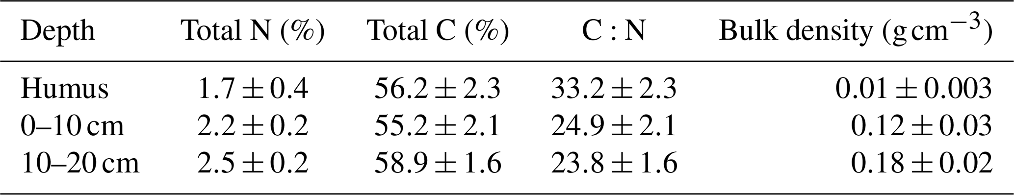
The flux measurements were conducted between 1 June 2015 and 29 September 2019 in a drained nutrient-rich peatland forest located in southern Finland (Lettosuo, 60°38^′ N, 23°57^′ E). The mean annual temperature in the area is 5.2 °C and the mean annual precipitation 621 mm according to the long-term weather record from the nearest automatic weather station (Jokioinen–Ilmala, 1991–2020, 35 km from the study site). The site was initially drained in the 1930s and more intensively in 1969 to promote tree growth. Ditches were dug about 1 m deep and 45 m apart. The site was fertilized with phosphorus and potassium after the later drainage. Drainage lowered the groundwater table, resulting in a transition to boreal-forest-like vegetation. The relatively low C:N ratio reflects the fen history of the site (Table 1).

Table 1 Soil properties at the study site. Values represent general soil properties at the study site before the selection harvest was done. Data from Korkiakoski et al. (2019).

Before March 2016, the site was a mixed forest with an overstory dominated by Scots pine (Pinus sylvestris) and an understory dominated by Norway spruce (Picea abies). Both overstory and understory contained a small amount of downy birch (Betula pubescens). Overstory pines were removed during a selection harvest in March 2016 (70 % of the total stem volume; Korkiakoski et al., 2020, 2023). The surroundings of the measurement chambers used in this study were harvested more lightly, and the chamber area continued to have a high coverage of spruce and birch. The selection harvest did not affect N₂O fluxes according to the previous study from the site (Korkiakoski et al., 2020), and the effect of the harvest was left out of the focus of this study.

2.2 Automatic chamber fluxes

The N₂O flux between the forest floor and the atmosphere was measured using six automated chambers. The transparent, acrylic, rectangular cuboid chambers with the dimensions $\mathrm{57}\times \mathrm{57}\times \mathrm{40}\mathrm{cm}$ (length × width × height) were placed to sample the spatial variation of the ground vegetation composition within an area of 15×20 m (Fig. 1). The chambers were placed on permanently installed steel collars that were inserted into the soil to a depth of 2 cm. All the chambers closed for 6 min once an hour year-round. The chambers had an air temperature sensor and a fan to mix the air inside the chamber headspace. During winters, chambers were cleaned from snow and ice every 1–3 weeks, and snow depth inside the chambers was measured to account for the effect of snow depth on chamber volume. During the winter 2016–2017, extension collars were used to better allow snow to fit inside the chambers.

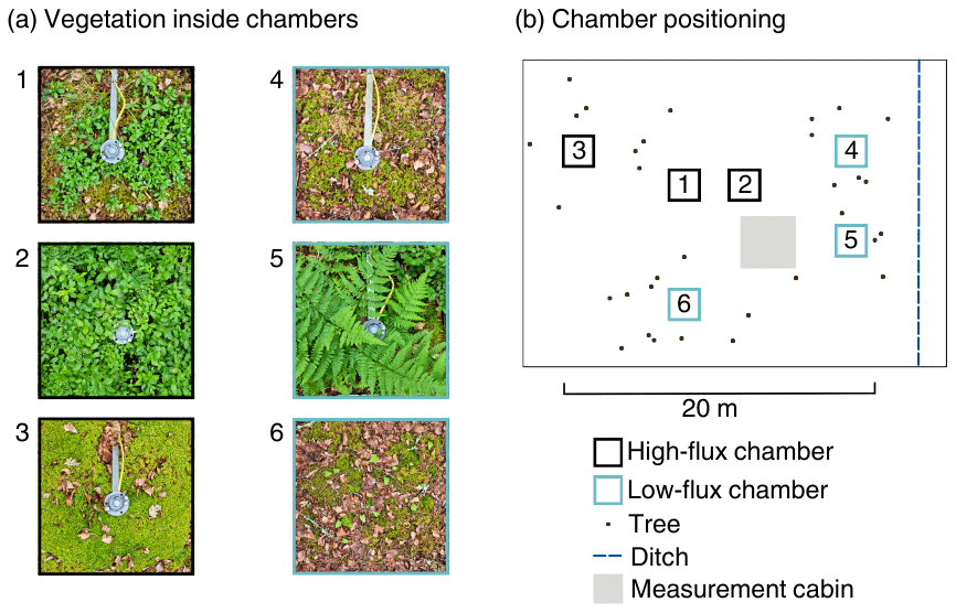
Figure 1 (a) Vegetation inside the six chambers and (b) the positioning of the chambers on the forest floor in relation to the nearest ditch and trees. Chambers are named from one to six based on the maximum measured flux with Chamber 1 having the highest measured flux. Chambers 1–3 with black edges are classified as “high-flux chambers” and Chambers 4–6 with blue edges as “low-flux chambers”. For more information on chamber vegetation, ditches and trees, see Table S1.

The N₂O concentration of the chamber headspace air was measured using a continuous wave quantum cascade laser absorption spectrometer (LGR-CW-QCL N₂O/CO-23d, Los Gatos Research Inc., Mountain View, CA, USA) that was placed in a measurement cabin close to the chambers (Fig. 1b). The analyzer had an accuracy of 0.01 ppb s⁻¹, corresponding to a minimum detectable flux (Nickerson, 2016) of 0.06 $\mathrm{\mu }\mathrm{g}{\mathrm{N}}_{\mathrm{2}}\mathrm{O}{\mathrm{m}}^{-\mathrm{2}}{\mathrm{h}}^{-\mathrm{1}}$ in our chamber system. During each chamber closure, air from the closed chamber was pumped into the analyzer and back to the chamber headspace through plastic tubes (length 15 m, flow about 1 L min⁻¹). After each chamber closure, the airflow was switched to the next chamber. Ambient air was measured for at least 1 min between the chamber closures to allow concentrations in the tubes to stabilize back to the ambient level. Concentration data from the first 30 s of each chamber closure were not used in flux calculation to avoid possible pressure disturbance caused by the closing chamber affecting the flux (Pavelka et al., 2018). For more information about the automatic chamber system, see the previous studies from the same site (Koskinen et al., 2014; Korkiakoski et al., 2017, 2020). Measurements in Chamber 6 ended 6 months earlier (April 2019) than measurements in other chambers due to problems in chamber functioning.

N₂O fluxes were calculated similarly to Korkiakoski et al. (2017) but by using a linear fit. The mean headspace temperature of the closure and air pressure measured at the site were used in the flux calculation. Calculated fluxes were filtered using normalized root mean square error and an iterative standard deviation filter to remove erroneous fluxes resulting from chamber malfunction (Korkiakoski et al., 2017). Daily mean N₂O fluxes from each chamber were used in the analysis because the automatic chamber system seemed to create an artificial diurnal cycle of N₂O from which the possible natural diurnal cycle could not be separated. The artificial diurnal cycle was caused by the difference in turbulence between the ambient air and chamber headspace, as previously reported for CO₂ and CH₄ (Koskinen et al., 2014; Korkiakoski et al., 2017). During calm periods, especially during summer nights, the transfer of N₂O from soil pores to the atmosphere slowed down, leading to increased N₂O concentration in the soil. When the chamber closed and the turbulence increased because of the fan, the N₂O from the soil pores was vented to the chamber headspace air, leading to overestimated flux. The opposite phenomenon probably occurred in windy conditions, resulting in underestimated flux. Based on our experience, automatic chamber fluxes measured in drained peatlands with dry and porous peat soil are particularly sensitive to this phenomenon (Koskinen et al., 2014; Korkiakoski et al., 2017). Hourly N₂O flux peaks were not typical in the flux data, and daily mean N₂O fluxes thus well represent the main characteristics of the temporal variation. It should be noted that the artificial diurnal cycle creates an additional source of uncertainty in the reported N₂O budgets.

2.3 Environmental variables

Several environmental variables were measured to link the temporal variation of N₂O fluxes with the environmental conditions. Air temperature was measured at 2 m height below the forest canopy (HMP45D, Vaisala Oyj, Vantaa, Finland). Soil surface temperature was measured at 2 cm depth in each chamber and the soil temperature at 5 cm depth at one location close to the chambers (Pt100, Nokeval Oy, Nokia, Finland). Soil moisture was measured at one location about 75 m from the chamber measurement location at 7 and 20 cm depths (Delta-T ML3, Delta-T Devices Ltd, Cambridge, UK). The soil moisture data were used to describe the temporal variation of soil moisture, assuming that the soil moisture had relatively similar temporal patterns across the study site. The absolute level of soil moisture in each chamber may have differed from the measured soil moisture, and the possibility of differences in the temporal variation of soil moisture between the logger and the chambers cannot be excluded. Soil moisture data were used together with water table level and precipitation data to strengthen the conclusions related to soil water conditions. The measurements of air and soil temperatures were ongoing throughout the study period, but the soil moisture measurements ended half a year earlier than automatic chamber measurements (April 2019).

Water table level (WTL) below the soil surface was measured using automatic loggers (TruTrack WT-HR, Intech Instruments Ltd, Auckland, New Zealand; Odyssey Capacitance Water Level Logger, Dataflow Systems Ltd, Christchurch, New Zealand). Chambers 1–2 and 4–5 shared a WTL logger that was placed between the chamber pairs. Chambers 3 and 6 had WTL loggers next to the chambers. WTL measurements for Chambers 3–6 started half a year later than chamber measurements (December 2015). WTL during this and other data gaps was modeled using random forest with conditional inference trees (Hothorn et al., 2006). WTL data from Chambers 1–2, seven other WTL loggers at the study site, and precipitation were used as explanatory variables in the gap-filling model. Modeling was done first for the logger with the least amount of missing data, after which the gap-filled WTL time series was added to the model as an explanatory variable to increase the predictive power of the model for the variables with more missing data (evaluation data R²=0.90–0.97).

Precipitation was measured at the site throughout the study period (Casella Tipping Bucket Rain Gauge, Casella Solutions Ltd, Bedford, UK; OTT Pluvio2 L 400 RH, OTT Hydromet Ltd, Kempten, Germany), and daily precipitation sum was calculated. The precipitation data measured at the nearest weather station were used to gap-fill winters and other measurement gaps in precipitation data (correlation of precipitation between sites 0.65, p<0.05). Snow depth measured at the nearest weather station was used to describe general snow conditions experienced each winter. Thermal seasons were used to analyze the seasonality of N₂O fluxes. The thermal seasons were defined according to typical Finnish standards (Ruosteenoja et al., 2016; Finnish Meteorological Institute, 2023) by using air temperature data from the site (Appendix A). Seasons based on months were used to compare conditions measured at the site with long-term averages reported monthly for the nearest weather station.

2.4 Identifying high-flux periods

The term “high-flux period” was used to describe periods of elevated flux, including periods from moderately increased flux to the highest flux peaks. “High-flux period” was used instead of a commonly used “hot moment” because the definition of a hot moment largely varies between studies, with sometimes only extremely high fluxes being considered as hot moments (Molodovskaya et al., 2012; Krichels and Yang, 2019; Anthony and Silver, 2021; Song et al., 2022).

To identify the high-flux periods, their length, seasonality, and starting conditions, different thresholds to separate high-flux days from the baseline days were tested. High fluxes were measured less frequently compared to the more common low fluxes (Fig. S1 in the Supplement). Any percentile threshold between 60 %–80 % separated high-flux days from the more common baseline fluxes relatively well, and the mean of these (70 %) was used. Days with the mean flux above the 70th percentile were classified as high-flux days and the rest of the days as baseline days. The length of each high-flux period was the number of days the flux remained above the 70th percentile, including possible data gaps within this period. The high-flux period was set to continue over a data gap if 3 d before and after the data gap were classified as high-flux days. A 3 d marginal was chosen to ensure that short 1–2 d peaks would not create long-lasting high-flux periods over data gaps. If the high-flux period started from a data gap or ended to it, the start or end date of the high-flux period was set to the first or last measured day, respectively. Pearson correlation was used to test how similar the temporal patterns of N₂O flux were between chambers.

2.5 Machine learning

Machine learning models were used to improve understanding of the temporal controls on N₂O flux, including a possible effect of time lags between environmental conditions and N₂O flux. The machine learning approach was used because machine learning models do not rely on mathematical functions to describe relationships between variables and are able to account for interactions between variables flexibly (Olden et al., 2008). The random forest algorithm, developed by Breiman (2001), is a classification tree-based method that uses bootstrap aggregation of a model training data and a randomly chosen subset of explanatory variables (mtry-parameter) to train each classification tree. In bootstrap aggregation, a subset of data is taken from the model training data with or without returning it to the original training data. The part of data that is not bootstrapped to train trees is called out-of-bag (OOB) data, and it can be used to evaluate model performance. In each random forest tree, the bootstrapped data are classified into subgroups and further into smaller subgroups by setting threshold values for the randomly chosen subset of explanatory variables. The setting of the threshold values is done to maximize the information gain until no further thresholds, also called splits, can be made. After a selected number of trees are built, the final model prediction can be made using the average of all the trees (continuous response) or the most common outcome (categorical response).

Random forest variable importance (VI) metrics show the importance of each explanatory variable in explaining variation in the response variable. VI metrics can be biased if the explanatory variables correlate (Strobl et al., 2007). Therefore, we used random forest with conditional inference trees (Hothorn et al., 2006) that allowed us to get more accurate VIs in the presence of correlated explanatory variables and their time-lagged versions. Compared to trees in random forest, conditional inference trees use a p-value-based splitting criterion to classify the bootstrap aggregated data in the building phase of each tree. As suggested by Strobl et al. (2007), in the presence of correlated explanatory variables, variable importance metrics from the conditional inference trees were calculated using conditional permutation importance.

Chamber-specific models had daily mean N₂O flux as the response variable and the measured temperature variables (air, soil 2 and 5 cm depths), soil moisture (7 and 20 cm depths), WTL, and daily cumulative precipitation as explanatory variables. Periods of missing data in environmental variables were gap-filled using the random forest proximity tool RFimpute (Liaw and Wiener, 2002). One-to-seven days' time-lagged versions of each environmental variable were added as explanatory variables to the models besides unlagged environmental variables. The imbalanced distributions of N₂O fluxes were corrected with the SMOGN algorithm (Abd Elrahman and Abraham, 2013). The subset of data to train each tree was bootstrapped without replacement with a sample size 0.632 times the size of the training dataset, as suggested by Strobl et al. (2007). Models were trained with 500 trees, and random forest default mtry for continuous response variable was used ($\mathit{\text{mtry}}=\text{number of explanatory variables}/\mathrm{3}$).

The first 3 years of data were utilized as the model training period (June 2015–June 2018), and these data were further split into 70 % training data and 30 % evaluation data to test model performance within the training period. The fourth year of measurements until soil moisture measurements ended (June 2018–April 2019) was left aside for evaluation to test model performance outside the training period. The performance of the models on different evaluation datasets was analyzed using R squared (R²) and root mean squared error (RMSE). R² was used to compare model performance between chambers. Variable selection was not done. Evaluation results are presented in appendices (Appendix B).

VIs and accumulated local effects (ALEs) were used to interpret the modeling results. For easier comparison of VIs across chambers, the VIs of each chamber were scaled from zero to one (0 = least important variable, 1 = most important variable), and the total VIs of each variable were calculated (total VI = VI of unlagged variable + VIs of lags). The ALE method by Apley and Zhu (2020) was used to visualize the response of N₂O flux to environmental conditions and their lags in the models. In ALE figures, ALE value (y axis) zero refers to the mean predicted N₂O flux, with a positive ALE value meaning larger and a negative value lower predicted N₂O flux in a specific environmental condition (x axis). ALE values for lagged environmental variables indicate the response of predicted N₂O flux to previous environmental conditions. From the unlagged and lagged versions of each environmental variable, the one that received the highest ALE value for a given environmental condition was considered to represent the typical response time of N₂O flux to that condition. In this article, the response time, or lag length in the presence of at least a 1 d lag, refers to the time it takes for N₂O to reach peak flux after the onset of a given environmental condition. The reported evaluation results (RMSE, R²), VIs, and ALE values are averages over 10 model runs.

2.6 N₂O budgets

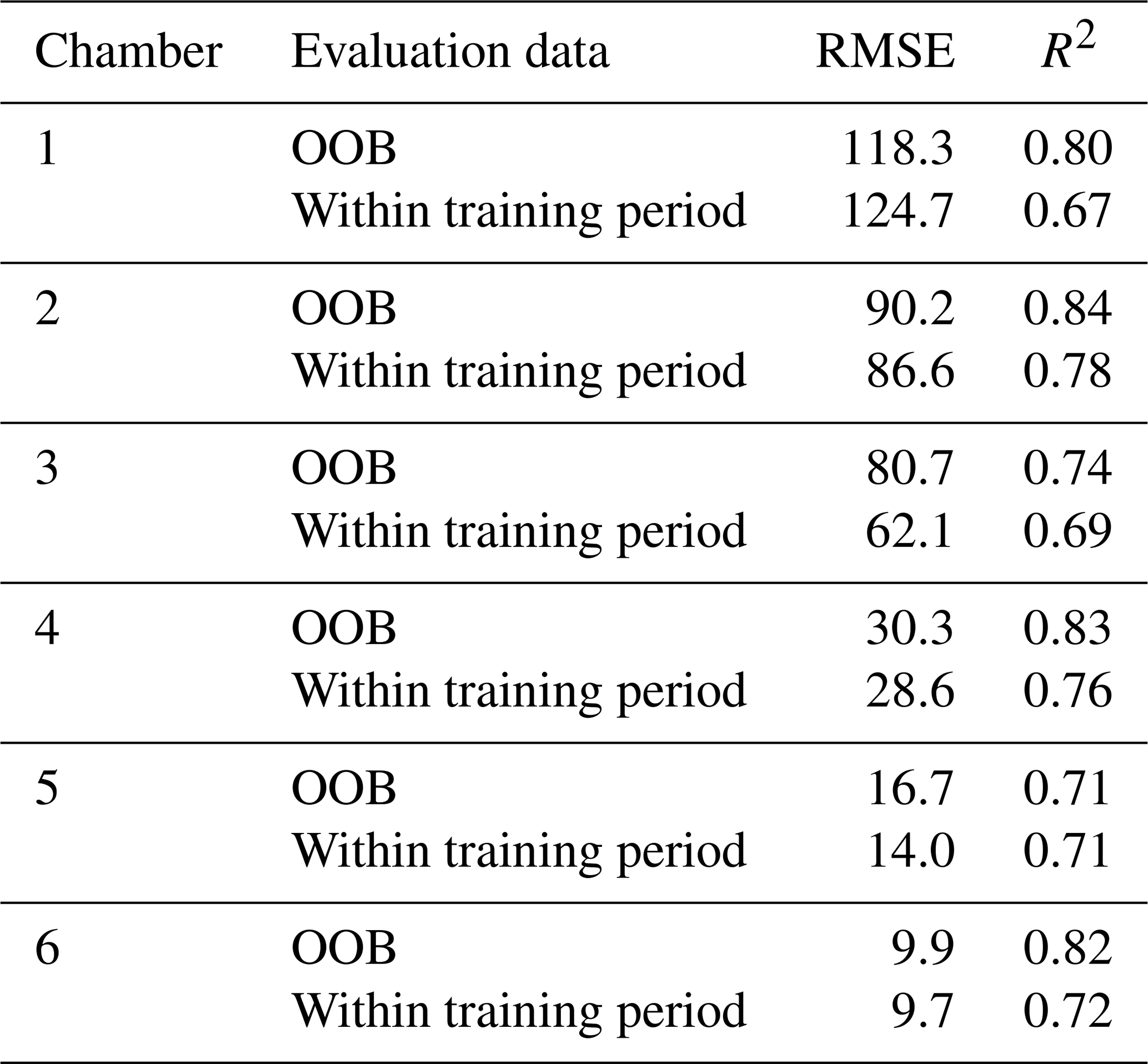
Data gaps covered 12 %–24 % of the study period depending on the chamber. Daily mean N₂O flux time series were gap-filled to calculate N₂O budgets. Gap-filled data were not used in other analyses to avoid additional uncertainty arising from the gap-filling. The same models and explanatory variables were used as in the machine learning part, including time-lagged variables. The fourth measurement year previously left for evaluation was also included in the training data for gap-filling. To test the performance of the gap-filling model, separate models were run with 70 % and 30 % split to the training data and evaluation data, respectively. Evaluation metrics (RMSE, R²) of gap-filling models are shown in the Appendix (Appendix B). Gap-filled daily mean N₂O fluxes were used to calculate N₂O budgets for each chamber in each thermal season. The uncertainty related to the N₂O budgets was assumed to be a combination of uncertainty related to flux measurement and uncertainty related to gap-filling. Detailed information about the calculation of the uncertainty can be found in Korkiakoski et al. (2017).

Flux calculation was performed in the Python programming language version 2.7 (Van Rossum and Drake, 1995). Data preparation and analysis were performed in R statistical software version 4.0.5 (R core team, 2021). Cforest command in the party package (Hothorn et al., 2006; Strobl et al., 2007; Zeileis et al., 2008) was used to perform random forest with conditional inference trees. Data and simplified R code about the machine learning part of the study are made freely available (Rautakoski et al., 2023; Rautakoski, 2024).

3 Results

3.1 Environmental conditions

The summers (June, July, August) 2015 and 2017 were colder (seasonal means 14.1 and 14.4 °C, respectively) than the long-term average (15.6 °C, Jokioinen–Ilmala 1991–2020), and winters (December, January, February) 2015–2016, 2016–2017, and 2018–2019 were warmer (seasonal means −3.4, −3.0 and −3.5 °C, respectively) than the long-term average (−4.3 °C) (Fig. 2). Temperatures were warm in all seasons in 2018 and 2019, with the summer (seasonal mean 17.2 °C) and autumn (seasonal mean 6.7 °C) 2018 being particularly warm compared to the long-term averages (summer 15.6 °C and autumn 5.4 °C). The area received the least amount of precipitation in 2018 (annual sum 434 mm) and the most precipitation in 2017 (annual sum 657 mm) with the long-term annual average being 621 mm. The summer 2018 (seasonal sum 44 mm) was especially dry compared to the long-term average summer precipitation of 71 mm. The drought that began in the spring 2018 continued until autumn.

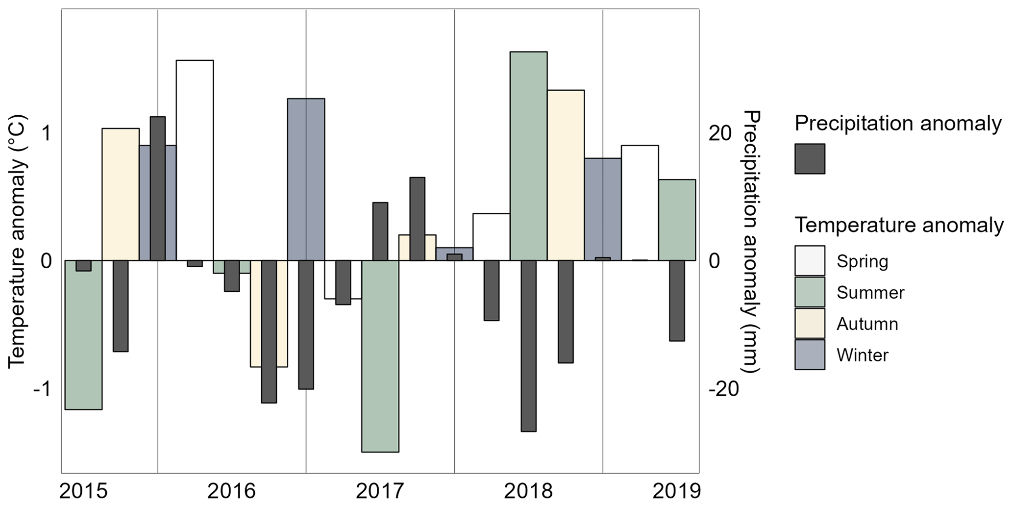
Figure 2 Difference of seasonal mean air temperature and precipitation sum from the long-term average. The long-term averages from the nearest weather station are used (Jokioinen–Ilmala, 1991–2020). Seasons are based on months (autumn: September–November, winter: December–February, spring: March–May and summer: June–August).

Soil moisture was continuously lower than the mean of the study period from the summer 2018 until the end of the study period (Fig. 3), with the study period mean being 0.28 ${\mathrm{m}}^{-\mathrm{3}}{\mathrm{m}}^{-\mathrm{3}}$ for 7 cm soil moisture and 0.56 ${\mathrm{m}}^{-\mathrm{3}}{\mathrm{m}}^{-\mathrm{3}}$ for 20 cm soil moisture. WTL was on average −36 cm and continuously deeper than that in the summer and autumn 2015 as well as in the summers 2018 and 2019. Soil temperatures at 5 cm depth reached freezing temperatures in winters 2015–2016 (min. −3.8 °C), 2016–2017 (min. −1.8 °C), and 2017–2018 (min. −0.33 °C). Variation of air and soil surface temperatures was high in winters 2015–2016 and 2016–2017. The snow cover was thickest in winter 2018–2019 (max. 52 cm) and thinnest in winter 2016–2017 (max. 11 cm). The number of days with snow cover was lower in winters 2015–2016 (85 d) and 2016–2017 (93 d) and higher in winters 2017–2018 (125 d) and 2018–2019 (116 d).

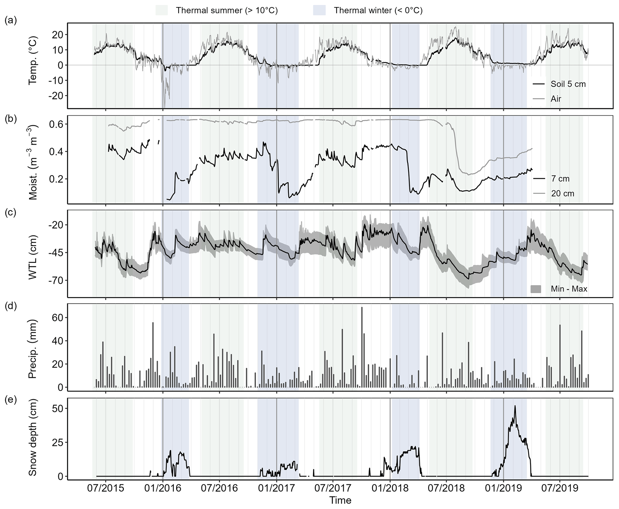
Figure 3 (a) Daily mean air and soil temperatures (5 cm depth), (b) soil moisture (7 and 20 cm depths), (c) water table level (WTL), (d) weekly precipitation sum, and (e) daily mean snow depth. WTL is the mean of the chambers with gray shading showing the range of WTL between different chambers. Snow depth was measured at the nearest weather station. Data are not gap-filled.

3.2 Temporal and spatial variation of N₂O flux

The daily mean N₂O flux varied between −10 and +1760 $\mathrm{\mu }\mathrm{g}{\mathrm{N}}_{\mathrm{2}}\mathrm{O}{\mathrm{m}}^{-\mathrm{2}}{\mathrm{h}}^{-\mathrm{1}}$ during the 4.5 years of measurements (Fig. 4). Three chambers (Chambers 1, 2 and 3) had maximum daily mean fluxes greater than 1100 $\mathrm{\mu }\mathrm{g}{\mathrm{N}}_{\mathrm{2}}\mathrm{O}{\mathrm{m}}^{-\mathrm{2}}{\mathrm{h}}^{-\mathrm{1}}$, and the other three chambers (Chambers 4, 5 and 6) had maximum daily mean fluxes less than 400 $\mathrm{\mu }\mathrm{g}{\mathrm{N}}_{\mathrm{2}}\mathrm{O}{\mathrm{m}}^{-\mathrm{2}}{\mathrm{h}}^{-\mathrm{1}}$ (Table 2). Chambers 1–3 also had a higher mean flux than Chambers 4–6 in all years (Table S2 in the Supplement). The annual mean flux was the highest in 2016 or 2017, depending on the chamber, and lowest in 2018 or 2019. Based on the differences in the maximum flux, standard deviation, and the range of the flux variation, Chambers 1–3 were classified as “high-flux chambers” and Chambers 4–6 as “low-flux chambers”.

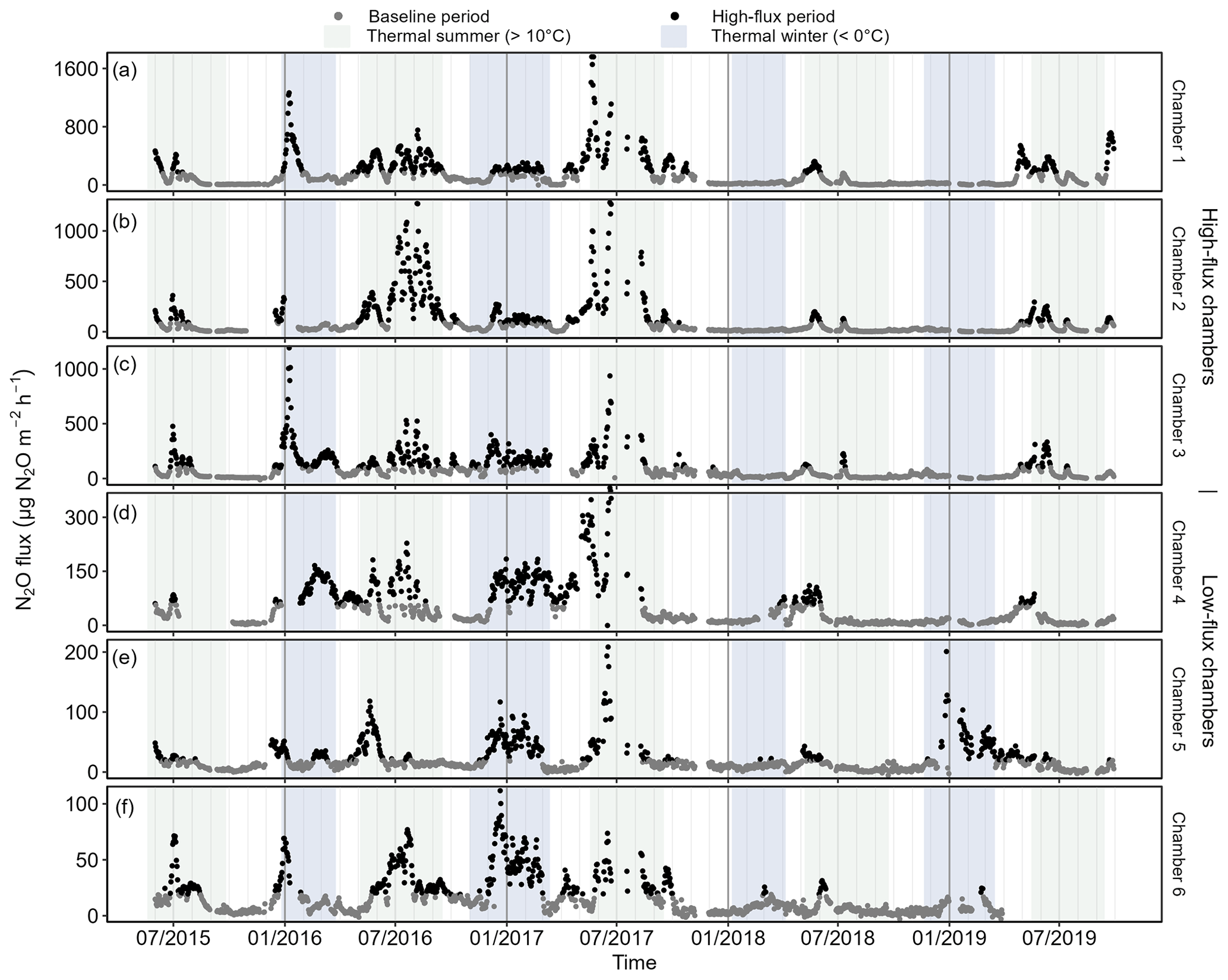
Figure 4 Daily mean N₂O flux measured in the six automatic chambers in 2015–2019. Fluxes from different chambers are shown in panels (a–f) ordered by maximum daily mean N₂O flux. Chambers are grouped into high-flux (Chambers 1, 2, and 3) and low-flux chambers (Chambers 4, 5, and 6). The scale of the y axis is chamber-specific, and fluxes are not gap-filled. Periods with the daily mean fluxes > 70th percentile are classified as high-flux periods.

Table 2 Minimum, maximum, mean, median, 70th percentile, and standard deviation (SD) of daily mean N₂O fluxes over the study period. The unit of the flux is $\mathrm{\mu }\mathrm{g}{\mathrm{N}}_{\mathrm{2}}\mathrm{O}{\mathrm{m}}^{-\mathrm{2}}{\mathrm{h}}^{-\mathrm{1}}$. Percentile thresholds (70 %) were used to define high-flux periods. Year-specific statistics can be found in Table S2.

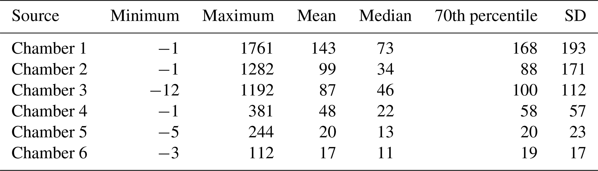
The chamber-specific 70th percentiles that were used to define the high-flux periods from the baseline periods ranged from 20 (Chamber 5 and 6) to 170 $\mathrm{\mu }\mathrm{g}{\mathrm{N}}_{\mathrm{2}}\mathrm{O}{\mathrm{m}}^{-\mathrm{2}}{\mathrm{h}}^{-\mathrm{1}}$ (Chamber 1, Table 2). The length of the individual baseline periods varied from 1 to 330 d with a mean of 26 d, while the length of the high-flux periods varied between 1 and 134 d with the mean of 11 d. The correlation of flux time series between chambers varied between 0.79 (Chambers 1 and 2) and 0.29 (Chambers 1 and 4) (Table S4). Correlation was the highest between the chambers with a similar range of N₂O flux: among high-flux chambers, correlation varied between 0.64–0.79 and among low-flux chambers, between 0.46–0.49. Differences in WTL between chambers were statistically significant but were not associated with the spatial variation of N₂O flux.

3.3 Seasonality of N₂O flux

The highest N₂O fluxes were measured during thermal summers (Chambers 1, 2, 4 and 5) or winters (Chambers 3 and 6). The fluxes were also on average the highest in summers and winters and the lowest in autumns (Tables S3). The percentage of measurement days identified as high-flux days averaged 24 % in spring, 38 % in summer, 44 % in winter, and 9 % in autumn (Fig. 5). The highest proportion of winter and summer high-flux days were measured in 2016 and 2017 and the lowest proportion in 2018.

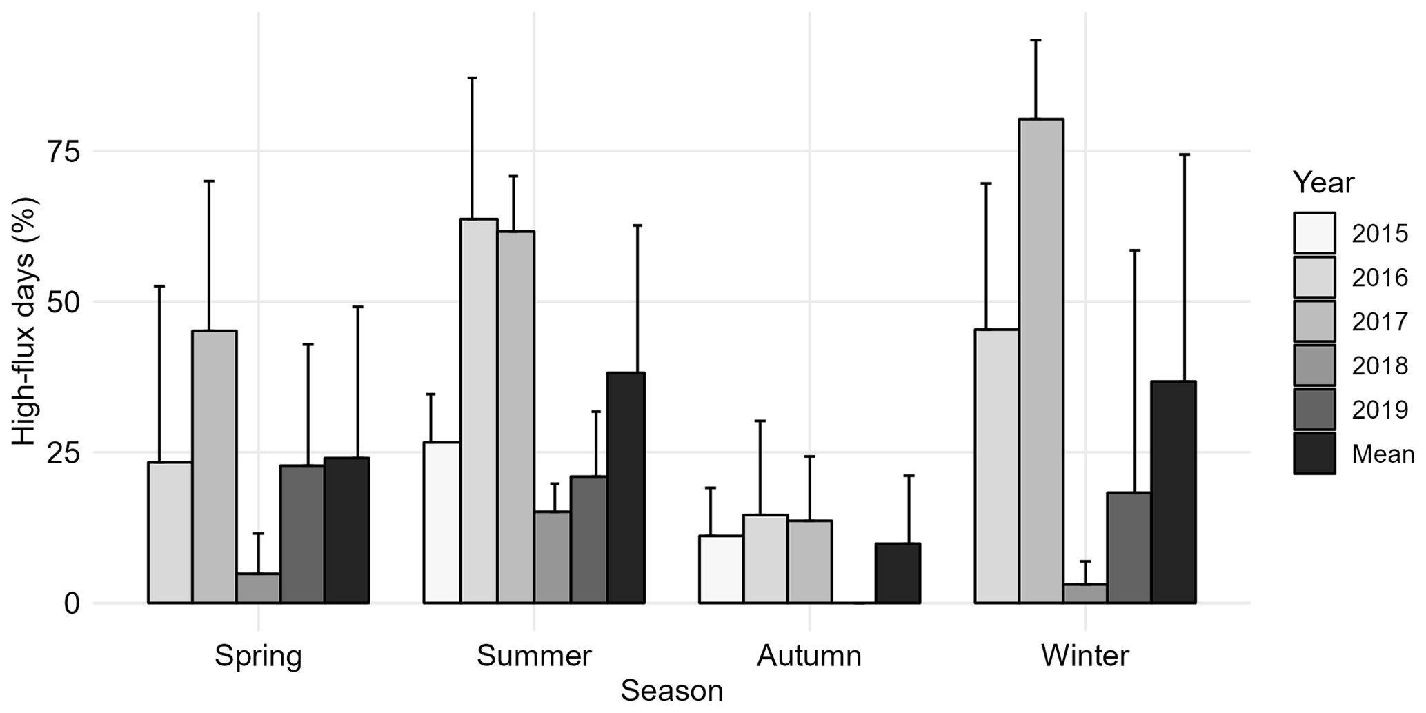
Figure 5 Occurrence of high-flux days out of measured days in different thermal seasons. Bars show annual means across different chambers, and error bars show standard deviation between chambers. Mean bars show the mean across the years. The bar for winter 2019 only contains winter days between January–March 2019.

In spring, N₂O fluxes increased steadily as soil surface temperatures increased above zero (Figs. 6 and S2–S6), with most of the spring high-flux periods starting at soil surface temperatures 0–2 °C (Fig. 7). Spring N₂O fluxes increased steadily with increasing soil temperatures, and flux peaks were reached in late spring or early summer. Summer high-flux periods started after precipitation events at moist soil conditions (0.37–0.41 ${\mathrm{m}}^{-\mathrm{3}}{\mathrm{m}}^{-\mathrm{3}}$) and during relatively high WTL (−35 to −50 cm depth) (Fig. 7), but the peak fluxes were reached several days after the rain events. The starting conditions for soil moisture and WTL in the autumn high-flux periods were similar to those in summer, but the response to soil wetting was slower and fluxes were smaller.

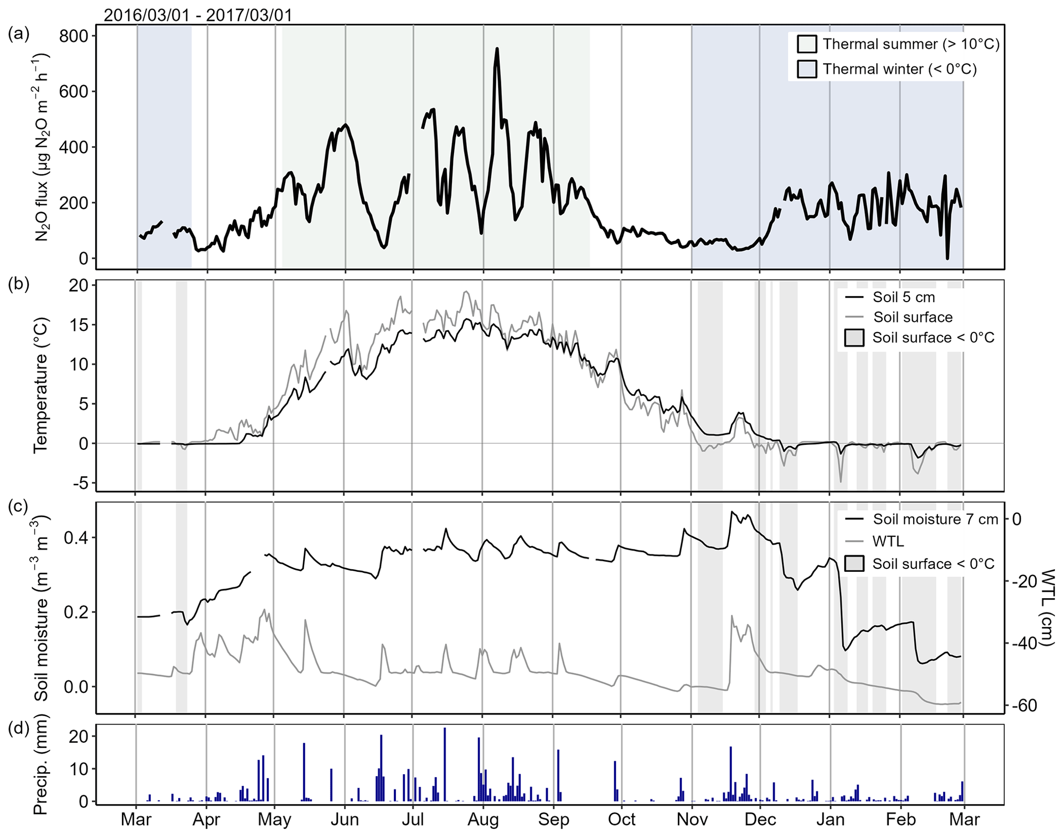
Figure 6 (a) Daily mean N₂O flux, (b) soil surface temperature and temperature at 5 cm depth with highlighted freezing periods (soil surface temperature < 0 °C), (c) soil moisture and water table level (WTL), and (d) daily precipitation from March 2016 to March 2017 in Chamber 1. The temporal variation of N₂O flux in Chamber 1 was similar to the other chambers, but the range of flux variation was larger compared to the low-flux chambers. The shown temporal dynamics of N₂O flux were measured in a year with relatively wet summer and warm winter. Data are not gap-filled. Figures for other chambers are presented in the Supplement (Figs. S2–S6).

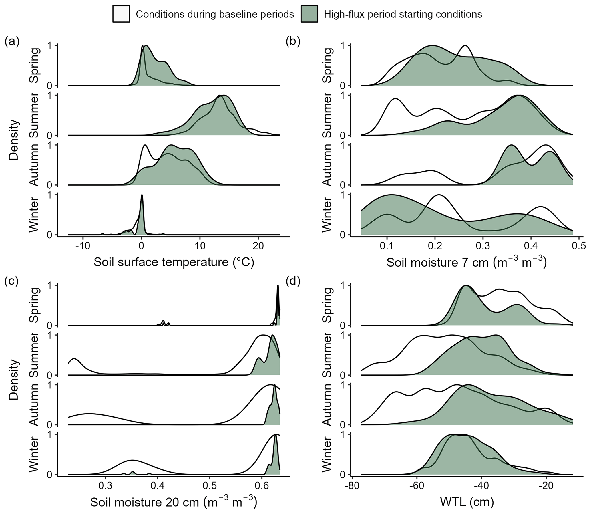
Figure 7 High-flux period starting conditions in each season compared to conditions outside the high-flux periods. Density plots show the distribution of high-flux periods starting on different (a) soil surface temperature, (b) soil moisture at 7 cm depth, (c) soil moisture at 20 cm depth, and (d) water table level (WTL). The y axis shows scaled (0–1) proportion (%) of high-flux periods starting on conditions shown on the x axis (1 = most common high-flux periods starting condition, 0 = no starting high-flux periods). For comparison, the variation in soil conditions during baseline periods is also shown (1 = most common baseline period condition, 0 = no such condition measured during baseline periods). All years and chambers are included.

Winter high-flux periods started on soil temperatures close to 0 °C (Fig. 7). In early winter, N₂O fluxes increased when soil surface temperatures decreased to near zero and below that, with further increase in flux measured if soil temperature also at 5 cm depth decreased below zero (Figs. 6 and S2–S6). Later in the winter, increased N₂O fluxes were measured during periods of soil freezing or when soil temperatures increased towards or above zero. Freezing of the soil surface did not typically lead to high N₂O fluxes without temperatures being below zero also at 5 cm depth. The response to soil freezing, especially in the early winter, was stronger than the response to soil thawing in terms of duration of the high-flux periods and peak flux.

3.4 Machine learning

Soil moisture (both 7 and 20 cm), air temperature, and WTL were considered to be the most important variables explaining the temporal variation of N₂O flux (Fig. 8) with the mean total variable importance (VI, 0 = no importance, 1 = high importance) being 0.7 and 0.6 for soil moisture (7 and 20 cm respectively) and 0.5 for air temperature and WTL. The mean VI of lags (1–7 d) for each environmental variable was the highest for 7 and 20 cm soil moisture (mean VI 0.3 for both) with 5 cm soil temperature and air temperature also having importance on lags (mean VI 0.25 and 0.20, respectively, Figs. S8–S12). Lags of other variables received mean VIs lower than 0.1, but precipitation had an increasing VI towards the longest lags (6–7 d).

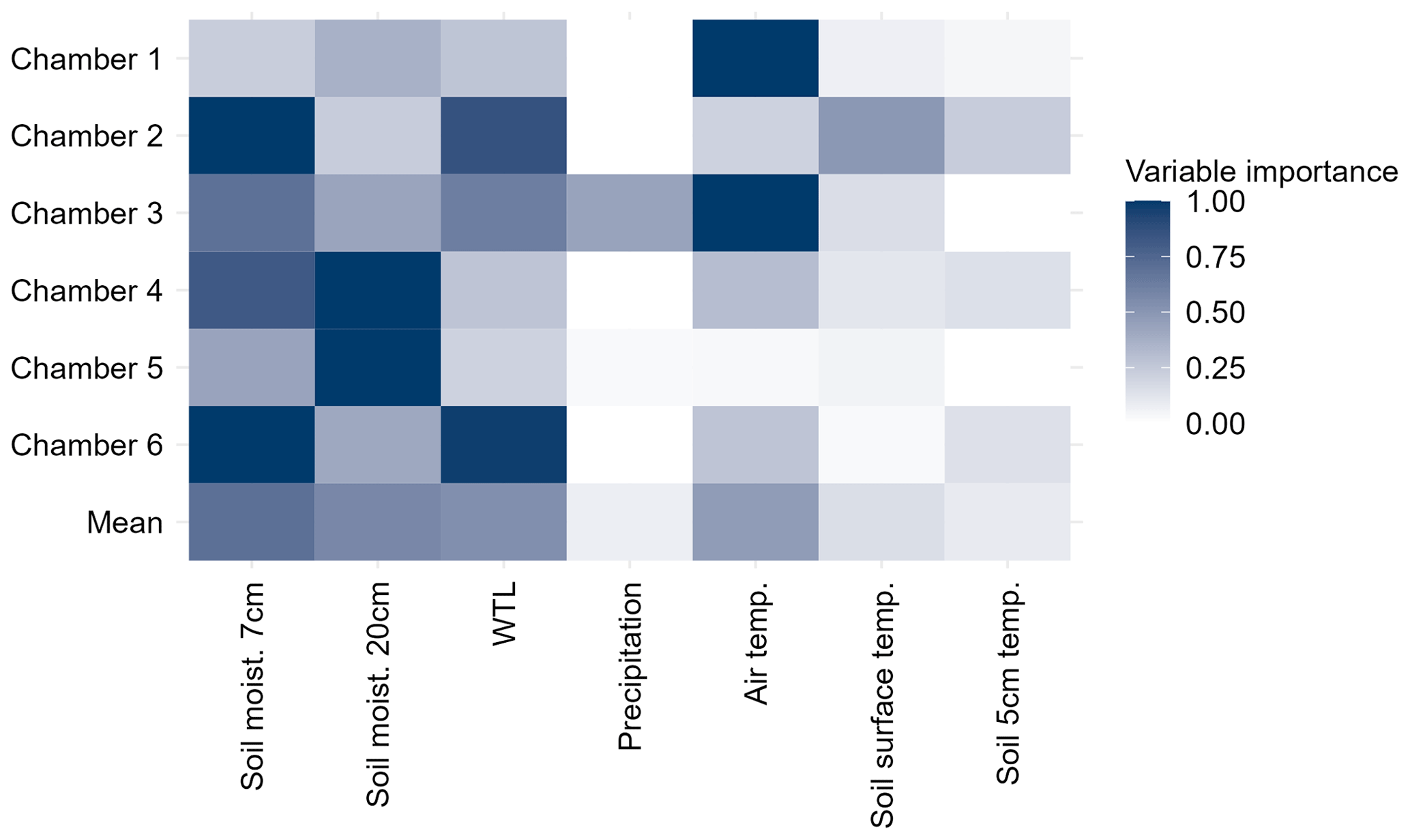
Figure 8 Total variable importance (VI) of different environmental variables in explaining the temporal variation of N₂O flux in random forest with conditional inference trees. Total VI is the sum of VIs of unlagged and lagged (1–7 d) versions of the variable. Rows in the matrix plot show VIs for different chambers and the mean VIs across all the chambers (Mean). VI scores are scaled between 0 and 1 (0 = no importance, 1 = highest importance) per chamber. Lag-specific VIs are shown in Fig. S7.

Accumulated local effects (ALEs) for 7 cm soil moisture showed that the highest fluxes were predicted for the 1–7 d lagged soil moisture when the soil was moist (> 0.35 ${\mathrm{m}}^{-\mathrm{3}}{\mathrm{m}}^{-\mathrm{3}}$). The lag with the highest predicted flux varied from 1 to 7 d between chambers with a mean lag of 4 d. Predicted fluxes were also high when soil moisture was low (< 0.1 ${\mathrm{m}}^{-\mathrm{3}}{\mathrm{m}}^{-\mathrm{3}}$, frozen soil). For WTL, the predicted flux was generally high when WTL was high (> −45 cm), with the highest predicted flux on average for 4 d lagged WTL. The predicted flux for unlagged WTL was low at high WTL, while the predicted flux for unlagged WTL increased with decreasing WTL. N₂O flux was predicted to be the highest 4–7 d after precipitation with an average lag of 5 d between chambers when daily precipitation had been at least 5 mm.

For air and soil surface temperatures above 5 °C, the predicted fluxes increased with increasing temperature, with the highest predicted fluxes at air temperatures above 15 °C and soil temperatures above 10 °C. For air and soil temperatures (soil surface and 5 cm depth) below 0–2 °C, the predicted N₂O fluxes increased with decreasing temperature. In most chambers, the increase in predicted flux for soil 5 cm temperature at 0–2 °C was particularly strong. Responses between lagged and unlagged temperatures varied among chambers.

3.5 N₂O budgets

The annual N₂O budgets of individual chambers varied between 60 (Chamber 6) and 2110 $\mathrm{mg}{\mathrm{N}}_{\mathrm{2}}\mathrm{O}{\mathrm{m}}^{-\mathrm{2}}{\mathrm{yr}}^{-\mathrm{1}}$ (Chamber 1) when considering the three full measurement years 2016, 2017, and 2018 (Fig. 10 and Tables S5–S9). In 2016 and 2017, annual N₂O budgets were 1120–2110 $\mathrm{mg}{\mathrm{N}}_{\mathrm{2}}\mathrm{O}{\mathrm{m}}^{-\mathrm{2}}{\mathrm{yr}}^{-\mathrm{1}}$ in the high-flux chambers and 200–740 $\mathrm{mg}{\mathrm{N}}_{\mathrm{2}}\mathrm{O}{\mathrm{m}}^{-\mathrm{2}}{\mathrm{yr}}^{-\mathrm{1}}$ in the low-flux chambers. In 2018, the N₂O budgets were lower than 400 $\mathrm{mg}{\mathrm{N}}_{\mathrm{2}}\mathrm{O}{\mathrm{m}}^{-\mathrm{2}}{\mathrm{yr}}^{-\mathrm{1}}$ in all chambers. Winters and summers generally contributed the most to the annual N₂O budgets in all 3 years, with summers contributing on average 48 % and winters 34 % (Tables S5–S9). The contributions of spring and autumn to the annual N₂O budgets were on average 10 % per season.

4 Discussion

The measured N₂O fluxes were relatively high compared to fluxes reported for other boreal and temperate forests on peat and mineral soils. The N₂O budgets of boreal peatland forests have mainly varied between 30 and 1200 $\mathrm{mg}{\mathrm{N}}_{\mathrm{2}}\mathrm{O}{\mathrm{m}}^{-\mathrm{2}}{\mathrm{yr}}^{-\mathrm{1}}$ (Arnold et al., 2005; Minkkinen et al., 2020; Butlers et al., 2023) and in a similar range also in temperate mineral soil forests (Papen and Butterbach-Bahl, 1999; Luo et al., 2012). The N₂O budgets of our six automatic chambers are unlikely able to represent the N₂O budget of the whole site, but the mean annual N₂O budget of the chamber area greater than 950 $\mathrm{mg}{\mathrm{N}}_{\mathrm{2}}\mathrm{O}{\mathrm{m}}^{-\mathrm{2}}{\mathrm{yr}}^{-\mathrm{1}}$ in the two full study years out of three underlines the role of drained nutrient-rich peatland forest as hotspots for N₂O emissions (Fig. 10).

Nutrient-rich peat with a relatively low C:N ratio likely explains the high N₂O budgets of the chamber area. Low C:N ratio may also have increased the sensitivity of the N₂O flux to temporal variation in soil conditions (Klemedtsson et al., 2005; Pihlatie et al., 2010). Although the selection harvest done at the site in the spring 2016 did not increase the N₂O budget of the harvested area compared to the control site according to Korkiakoski et al. (2020), the effect of the harvest on N₂O fluxes of individual chambers cannot be completely excluded. Since the N₂O budgets increased after harvesting in both the harvested and the control site (Korkiakoski et al., 2020), most of the increase in N₂O budgets in the years 2016 and 2017 is likely explained by year-to-year variation in environmental conditions.

4.1 Seasonal variation of N₂O fluxes

Winters were characterized by N₂O flux peaks occurring during both freezing and thawing (Figs. 6, 7, and S2–S6), similar to those reported in earlier studies (Teepe et al., 2001; Maljanen et al., 2007, 2010). Freezing-related N₂O emissions are likely explained by N₂O production in the remaining unfrozen water films that have increased C and N content in the freezing soil (Maljanen et al., 2007; Congreves et al., 2018). Winter N₂O flux peaks were measured when soil frost reached at least the 5 cm depth, whereas during winters with only shallow frost (< 5 cm, winters 2017–2018 and 2018–2019), high N₂O fluxes were less common. This indicates the importance of frost depth for winter N₂O emissions. The importance of ground frost severity and depth has also been suggested by others in several ecosystems (Nielsen et al., 2001; Koponen and Martikainen, 2004; Maljanen et al., 2007; Luo et al., 2012). The importance of deeper soil freezing may indicate that the freezing-related N₂O fluxes mainly originate from the freezing peat rather than from the surface litter layer, unlike suggested by Pihlatie et al. (2007) in a nutrient-poor peatland forest. Low C:N ratio may have favored N₂O production in the nutrient-rich peat (Klemedtsson et al., 2005). Site-specific differences in nutrient availability may influence the sensitivity of winter N₂O fluxes to frost depth.

Winters with deeper soil frost and higher N₂O emissions (winters 2015–2016 and 2016–2017) were characterized by discontinuous and shallow snow cover and variable temperature conditions (Figs. 3 and 4). Shallow snow cover combined with alternating cold and warm weather in the first two winters of the study period has likely increased the number of freeze–thaw cycles and their intensity leading to higher total N₂O fluxes (Maljanen et al., 2007; Ruan and Robertson, 2017). The results suggest the possibility for increasing winter N₂O emissions from drained peat soils if winters continue to warm, the occurrence of extreme temperature fluctuations increases, and snow cover in the southern boreal region becomes shallower.

Similar to freezing, soil thawing triggered N₂O emissions during winter freeze–thaw cycles, but emissions ceased within a few days of the onset of the thawing phase even if soil temperature continued to rise (Figs. 6 and S2–S6). Similar short-term N₂O peaks in response to soil thawing have been measured also in laboratory experiments by Teepe et al. (2001) and Koponen and Martikainen (2004). Thaw-related emissions have often been explained by increased N availability in the thawing soil (Groffman et al., 2006; Wagner-Riddle et al., 2017), and the cause of the short pulse of N₂O flux during winter thawing might be related to the rapid use of labile N made available during the soil freezing period. Release of N₂O accumulated in the frozen soil might also explain some of the short-term N₂O flux peaks during thaw (Maljanen et al., 2007; Pihlatie et al., 2010). The response of N₂O fluxes to soil thaw during winter was weaker than the response especially to early winter soil freezing, which highlights the importance of freezing-related N₂O emissions in the studied ecosystem.

Previously, several studies on both peat and mineral soils have emphasized the importance of thaw-related spring N₂O fluxes in the annual N₂O budgets, with pronounced spring N₂O flux peaks in some cases accounting for a large fraction of the annual budget (Pihlatie et al., 2010; Luo et al., 2012; Wang et al., 2023). In the present study, spring soil thaw triggered N₂O emissions, but emissions increased slowly with increasing soil temperature and peaked in late spring or summer, significantly later after soil thaw than reported in previous studies (Figs. 6 and S2–S6). The strong temperature dependence of spring N₂O fluxes may indicate that the substrate for the spring N₂O production comes from the decomposing peat and litter in the warming soil. Temperature dependence of spring fluxes could be related to drained peat soil, where the major source of N is known to be decomposing peat (Martikainen et al., 1993). Different responses to thawing in winter compared to spring might be related to decreasing availability of N from early winter towards spring (Koponen and Martikainen, 2004; Congreves et al., 2018), which also likely explains the tendency for stronger response to freeze–thaw cycles in early winter.

High-flux periods during the growing season, especially in the summer, were associated with precipitation events that increased soil moisture and raised WTL (Figs. 6, 7 and S2–S6). These high-flux periods increased the total N₂O budget of the rainy summers (2016 and 2017), whereas the N₂O budget was low in the warm and dry summer 2018. Precipitation events may have increased the number of anoxic microsites in the soil, favoring N₂O production also through denitrification (Congreves et al., 2018). Fast peat decomposition in the warm soil during the summer likely reduced oxygen availability in the soil and increased N availability from the mineralizing peat resulting in high N₂O fluxes after summer rain events (Maljanen et al., 2003). Low N₂O fluxes during dry summer are likely explained by low microbial activity and substrate availability in the dry soil (Borken and Matzner, 2009; Congreves et al., 2018). Our results on summer and winter N₂O fluxes suggest that low N₂O fluxes during dry summers might offset the effect of the increasing winter N₂O fluxes on annual N₂O budgets if dry summers become more frequent in the warming climate.

N₂O fluxes during autumn were low and showed little year-to-year variability (Figs. 5, 6, and S2–S6). Low autumn N₂O emissions have also been measured in previous studies (Maljanen et al., 2003; Luo et al., 2012), although Pihlatie et al. (2007) and Alm et al. (1999) found increased autumn N₂O fluxes after litter fall in drained peatland forests. The low contribution of autumn N₂O fluxes to annual emissions in the present study is probably explained by the more nutrient-rich peat and the lower importance of N₂O production in the litter layer in the total N₂O production (Martikainen et al., 1993; Pihlatie et al., 2007). The results indicate that the site-specific differences in the peat nutrient availability could alter the contributions of different seasons to annual N₂O budgets. High temporal variability of fluxes and greater sensitivity of N₂O fluxes to environmental conditions in nutrient-rich peatland forests are likely to increase the sensitivity of N₂O budgets to increasing variability in seasonal conditions in the changing climate.

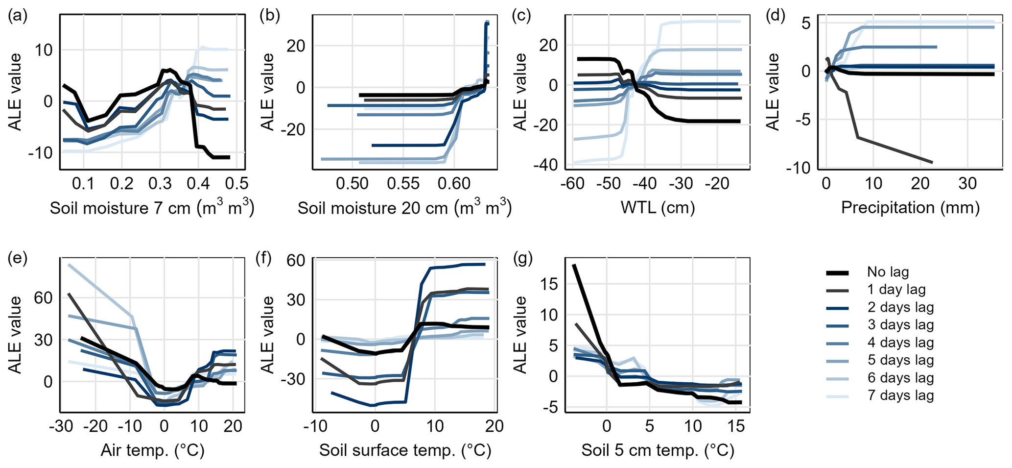
Figure 9 Response of predicted N₂O flux to different environmental conditions for Chamber 1 visualized using accumulated local effects (ALEs). Figures illustrate how the predicted N₂O flux values deviate from the mean predicted flux (ALE=0) along the gradients of (a) soil moisture at 7 cm depth, (b) soil moisture at 20 cm depth, (c) water table level (WTL), (d) precipitation, (e) air temperature, (f) soil surface temperature, and (g) soil temperature at 5 cm. ALE responses for unlagged and lagged variables (1–7 d) are included. ALE responses for Chambers 2–6 are presented in the Supplement (Figs. S8–12).

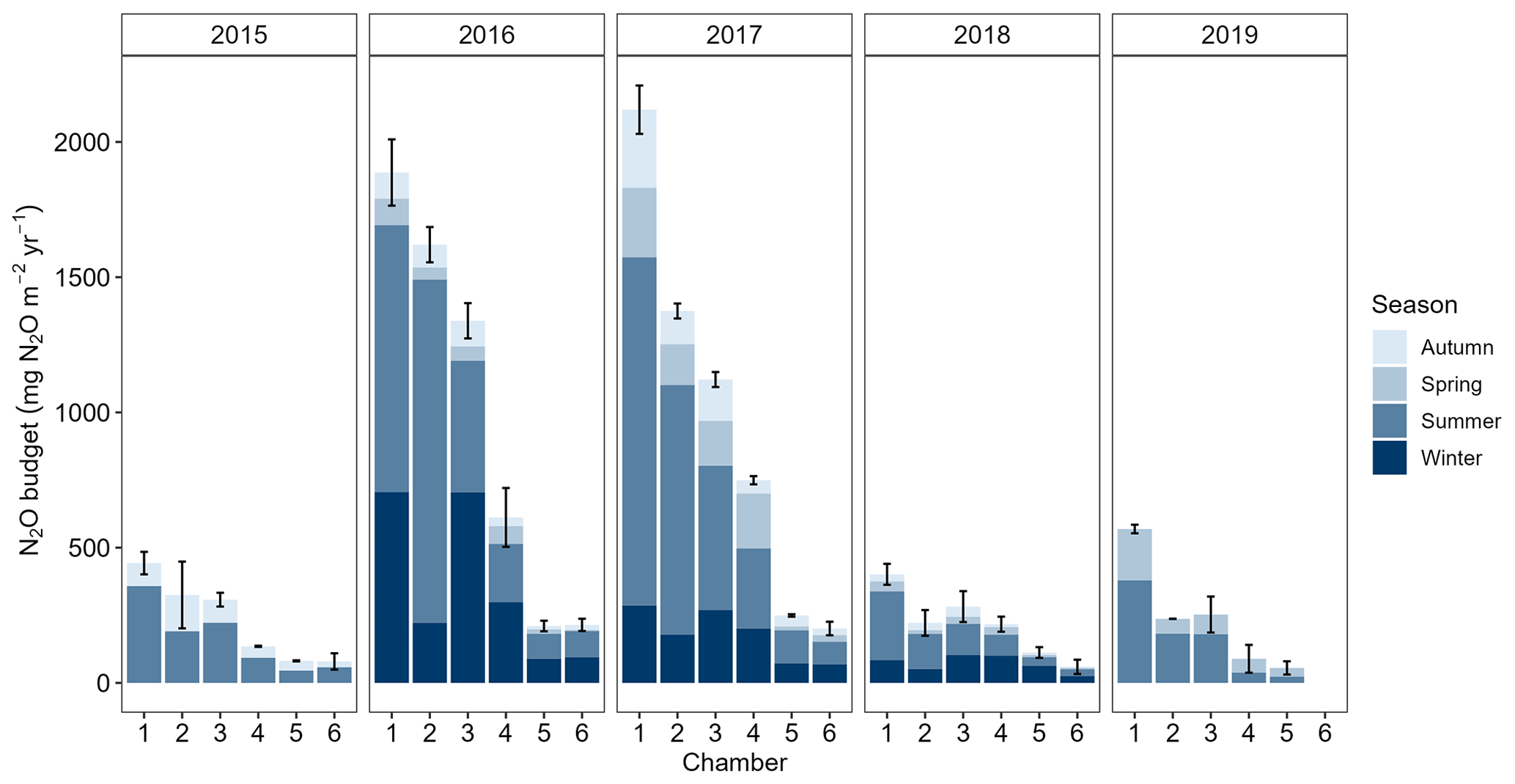
Figure 10 Annual N₂O budgets for each chamber and measurement year with seasonal contributions. The N₂O budget for 2015 only includes summer and autumn and the N₂O budget for 2019 spring and summer. Measurements in Chamber 6 ended in early 2019, and no budget is shown for that year. Thermal seasons are used. Error bars denote total uncertainty related to the total N₂O budget of the year.

4.2 Linkages to spatial variation

Lower fluxes from the three low-flux chambers (maximum flux < 400 $\mathrm{\mu }\mathrm{g}{\mathrm{N}}_{\mathrm{2}}\mathrm{O}{\mathrm{m}}^{-\mathrm{2}}{\mathrm{h}}^{-\mathrm{1}}$) compared to high N₂O fluxes (maximum flux > 1100 $\mathrm{\mu }\mathrm{g}{\mathrm{N}}_{\mathrm{2}}\mathrm{O}{\mathrm{m}}^{-\mathrm{2}}{\mathrm{h}}^{-\mathrm{1}}$) measured in the three high-flux chambers demonstrate the spatially variable nature of N₂O flux even on a small scale within a few meters (Groffman et al., 2009; Hénault et al., 2012; Jungkunst et al., 2012). What was notable was that the spatial differences in N₂O fluxes between chambers were persistent across years. The persistence of spatial variation implies that spatial variation of N₂O flux is controlled by long-term controls that persist throughout years with different weather conditions.

The long-term controls could include, for example, spatial variation in soil properties (e.g., pH, bulk density, availability of different forms of N) or placement of plant roots, both of which have been suggested to influence the spatial variation in N₂O fluxes even at very small scales within the soil (Butterbach-Bahl et al., 2002; Jungkunst et al., 2012; Kuzyakov and Blagodatskaya, 2015). In the present study, the high-flux chambers had fewer trees nearby than low-flux chambers, and the distance to nearby trees was greater (Fig. 1 and Table S1). Tree roots may have affected the availability of different forms of nitrogen through nitrogen uptake and nitrogen inputs to soil (Kaiser et al., 2011; Kuzyakov and Blagodatskaya, 2015; Hu et al., 2016), resulting in higher fluxes further away from the trees in this case. Because trees affect the forest floor microclimate, ground vegetation, and soil conditions through transpiration and by influencing the distribution of rainfall and light in the forest (Butterbach-Bahl et al., 2002; Aalto et al., 2022), variation in the tree cover may also have contributed to the spatiotemporal dynamics of N₂O fluxes. Although the distance to trees seemed to explain some of the spatial variation in N₂O flux, the spatial variation, especially within the small and high-flux chamber groups, remained unexplained. Ground vegetation was also not linked to spatial variation of N₂O. The results emphasize the importance of comprehensive soil sampling (e.g., N forms, bulk density, pH, C:N, root density) and chamber-specific measurements of environmental variables (e.g., soil moisture, soil temperature, WTL), when studying spatiotemporal variation of N₂O flux, especially in the forested study sites with variable microclimate.

Despite the large spatial variation in the N₂O flux, the high-flux periods identified for each chamber typically occurred at similar times, although the exact length and timing of the high-flux periods varied (Fig. 4 and Table S4). Similarities in the temporal variation of fluxes suggest that temporal changes in the soil environmental conditions affected N₂O fluxes relatively similarly across space. In previous studies, temporal patterns within sites were either variable or common across space (Velthof et al., 2000; Krichels and Yang, 2019), with both findings mainly attributed to the spatiotemporal variation of soil moisture. Stronger similarities in the temporal variation of N₂O flux within the low and high-flux chamber groups indicate that some differences in the response of N₂O flux to environmental conditions may be related to the overall spatial variation of the flux.

4.3 Delayed responses

The results indicate that N₂O flux has a delayed response to precipitation events with peak N₂O fluxes measured on average 4 d after soil moisture and WTL peaks and 5 d after rainfall (Figs. 9 and S8–S12). Studies mostly conducted on mineral soils in laboratories have found short time lags from the onset of anaerobiosis or water saturation to the highest measured N₂O production, with lags ranging from few hours to less than 2 d (Firestone and Tiedje, 1979; Smith and Tiedje, 1979; Russow et al., 2000; Song et al., 2019). Compared to the previous studies, the observed lag times are long, with indication for even longer lags than 7 d in some chambers.

The present data only allow us to hypothesize the causes of the long lag times after precipitation events. The ability of peat to retain moisture and thus anaerobic microsites in the soil means that anaerobic conditions for denitrification are maintained, and the possible co-occurrence of nitrification and denitrification can last for longer than in most mineral soils (Päivänen, 1973; Wrage et al., 2001; Walczak et al., 2002). The highest N₂O fluxes during the growing season were reached on intermediate soil moisture (0.3–0.4 ${\mathrm{m}}^{-\mathrm{3}}{\mathrm{m}}^{-\mathrm{3}}$) after the soil had started to drain and WTL had started to decrease after a precipitation event (Figs. 7, 9, and S8–S12). Based on this study and previous laboratory studies, we suggest that after a period of high N₂O reduction activity and therefore relatively low N₂O fluxes from denitrification in the wet soil soon after rain, N₂O production in the draining soil increased (Firestone and Tiedje, 1979; Russow et al., 2000; Congreves et al., 2018). As soil continued to drain, conditions for simultaneous nitrification and denitrification became optimal (Bateman and Baggs, 2005; Wang et al., 2021; Song et al., 2022), further increasing N₂O production and leading to the peak N₂O flux some days after rain. The ability of peat to retain moisture could extend the time for soil drainage after rainfall and thus time before optimal conditions for N₂O production are reached. Hydrophobic properties of dry peat soils can also extend the time before N₂O fluxes respond to soil wetting (Borken and Matzner, 2009) contributing to longer lag times. To determine exact lag times in response to soil moisture peaks, chamber-specific soil moisture data would be required.

Although models were not run for different seasons separately, the response of N₂O fluxes to precipitation events seemed to be slower during autumn and resulted in lower N₂O flux peaks (Figs. 6 and S2–S6). Lower temperatures in autumn likely decreased microbial activity and mineralization of N from decomposing peat, which could explain lower fluxes and slower response of N₂O fluxes to precipitation events in autumn (Holtan-Hartwig et al., 2002). Chamber differences in the lag times associated with precipitation events and differences in the variable importance of different environmental variables (Figs. 8 and S8–S12) may also indicate varying sensitivities of N₂O production to spatially varying soil conditions. These differences may be related to different microbial community, substrate availability, or soil properties that have been identified as important controls of N₂O production (Hénault et al., 2012; Butterbach-Bahl et al., 2013; Hu et al., 2015) and are likely to shape the response of N₂O production to environmental conditions.

5 Conclusions

This study shows high temporal and spatial variability in peatland forest N₂O fluxes with persistent spatial patterns across years with different environmental conditions. The temporal variation of N₂O flux was strongly influenced by seasonal weather conditions, especially precipitation, snow depth, and drought. Temporally varying soil conditions affect N₂O fluxes through complex responses that include delayed responses to soil wetting. Interactions between spatially and temporally varying soil conditions, such as temperature, further shape the spatiotemporal patterns of N₂O flux. The considerable small-scale spatial variation in N₂O fluxes is likely to be influenced by relatively long-term controls such as soil properties and positioning of trees.

The observed high N₂O fluxes from the peatland forest highlight the role of nutrient-rich drained peat soils as hotspots for N₂O emissions in the boreal region. The dependence of N₂O budgets on seasonally varying weather conditions suggests high sensitivity of peatland forest N₂O budgets to changing climate. Winter N₂O emissions will likely increase in the future due to warming winters with shallow and discontinuous snow cover. Summer N₂O emissions may decrease and possibly offset the effect of warming winters on annual N₂O budgets in dry years. Year-to-year variation in N₂O emissions will likely increase as extreme weather events are predicted to become more frequent.

Appendix A: Thermal seasons

Thermal winter was the season with daily mean air temperatures persistently below 0 °C and thermal summer season with daily mean air temperatures persistently above 10 °C (Ruosteenoja et al., 2016; Finnish Meteorological Institute, 2023). During spring and autumn, temperatures varied between 0–10 °C. Cumulative temperature sums of daily mean temperatures were then used to identify the starting days of the thermal seasons at which temperature went persistently above or below the seasonal temperature threshold (0 or 10 °C). The starting day of the thermal winter was the day after the annual cumulative temperature sum reached the maximum. The starting day of the thermal spring was the day after the minimum cumulative temperature sum was reached. Starting days of thermal summer and autumn were calculated similarly but by extracting 10 °C from the air temperatures before calculating the cumulative temperature sum (modified temperature sum). The day after the minimum modified temperature sum was reached was defined as the starting date of the summer, while the maximum modified cumulative temperature pointed to the onset of thermal autumn.

Appendix B: Evaluating the model performance

R₂ of the chamber-specific models used in the analyses varied between 0.72 and 0.85 in OOB data and between 0.60 and 0.69 in training period evaluation data (30 % of training period data) (Table B1). When predicting N₂O fluxes outside the training period (fourth measurement year), R₂ varied between 0.02 and 0.69. The performance of gap-filling models was tested only using OOB data and evaluation data within the whole study period (30 % of data). For gap-filling models, R₂ in OOB data varied between 0.71 and 0.84, while R₂ in evaluation data varied between 0.67 and 0.78 (Table B2).

Table B1 Model performance in evaluation datasets. Out-of-bag (OOB) data refer to data left outside model training in random forest with conditional inference trees. Evaluation data within the training period refer to 30 % of data randomly left aside for model evaluation. Evaluation data outside the training period refer to the fourth measurement year outside model training period.

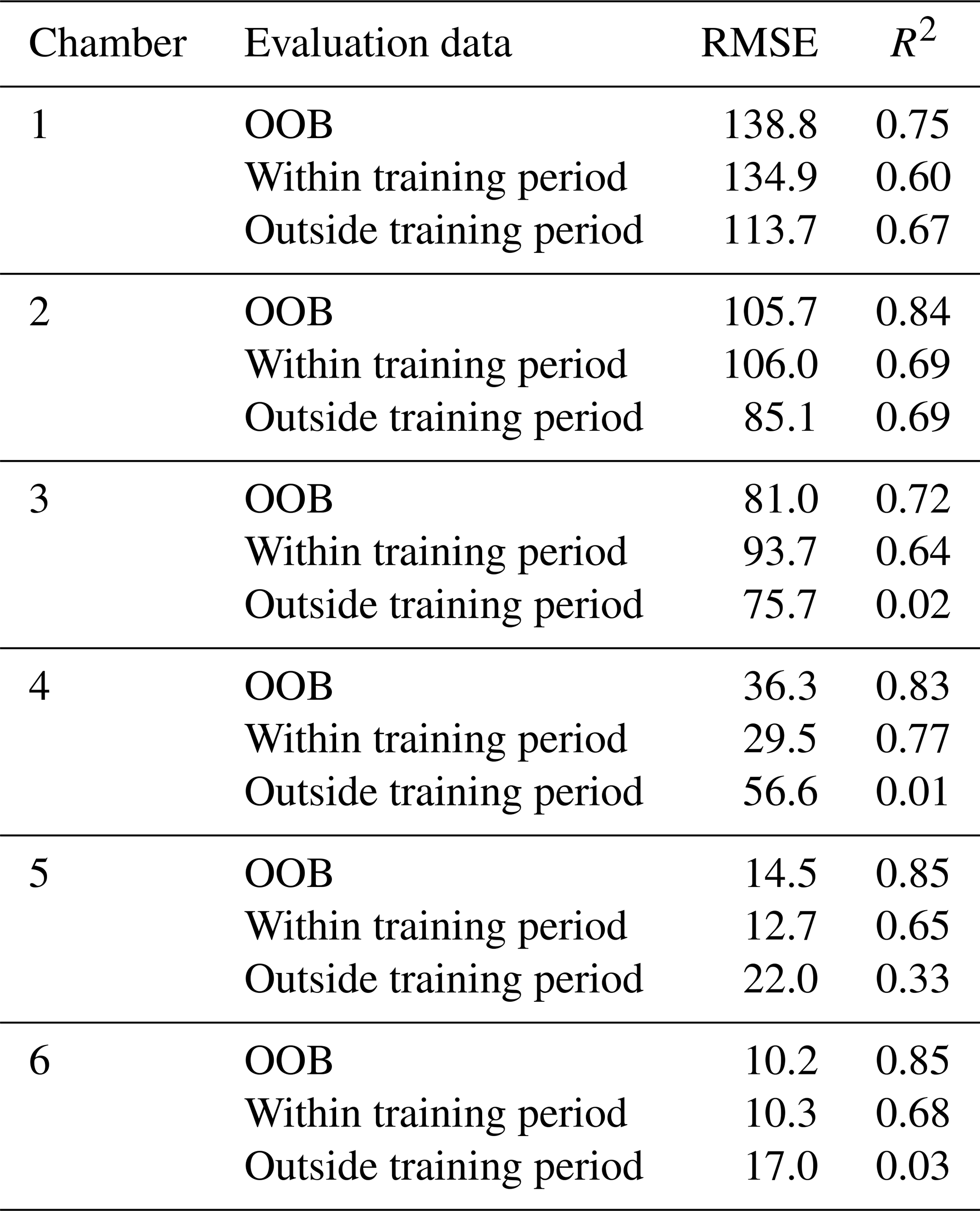
Table B2 Performance of gap-filling models on evaluation datasets. Out-of-bag (OOB) data refer to data left outside model training in random forest with conditional inference trees. Evaluation data within the training period refer to 30 % of training period data that were randomly left aside for model evaluation. The training period of gap-filling models covers the total study period (4.5 years).

For the models used in the analysis, the poor prediction accuracy outside of the training period, especially in Chambers 3, 4, and 6, was likely due to overestimation of the general flux level during the relatively dry year 2019, which was excluded from the training period (Fig. S13). The model was also unable to predict anomalous high-flux period in low-flux winter 2018–2019 in Chamber 5 likely due to a lack of chamber-specific soil temperature data deeper in the soil. The temporal patterns of the flux otherwise followed temporal patterns of measured fluxes relatively well. Poor prediction accuracy outside the training period in part of the chambers indicates that predicting N₂O fluxes to a year with distinct environmental conditions compared to the years in the training data may lead to large under or overestimation of N₂O fluxes. The used models could benefit from additional explanatory variables, such as redox potential or the availability of different forms of nitrogen (Rubol et al., 2012; Saha et al., 2021). Including additional soil variables in the model could decrease the need to have excessively large model training periods to accurately predict and gap-fill N₂O fluxes.