the Creative Commons Attribution 4.0 License.
the Creative Commons Attribution 4.0 License.
 | 25 Apr 2024
Interpretability of negative latent heat fluxes from eddy covariance measurements in dry conditions
Sinikka J. Paulus
Rene Orth
Sung-Ching Lee
Anke Hildebrandt
Martin Jung
Jacob A. Nelson
Tarek Sebastian El-Madany
Arnaud Carrara
Gerardo Moreno
Matthias Mauder
Jannis Groh
Alexander Graf
Markus Reichstein
Mirco Migliavacca
It is known from arid and semi-arid ecosystems that atmospheric water vapor can directly be adsorbed by the soil matrix. Soil water vapor adsorption was typically neglected and only recently received attention because of improvements in measurement techniques. One technique rarely explored for the measurement of soil water vapor adsorption is eddy covariance (EC). Soil water vapor adsorption may be detectable as downwardly directed (i.e., negative) EC latent heat (λE) flux measurements under dry conditions, but a systematic assessment of the use of negative λE fluxes from EC flux stations to characterize adsorption is missing. We propose a classification method to characterize soil water vapor adsorption, excluding conditions of dew and fog when λE derived from EC is not trustworthy due to stable atmospheric conditions. We compare downwardly directed λE fluxes from EC with measurements from weighing lysimeters for 4 years in a Mediterranean savanna ecosystem and 3 years in a temperate agricultural site. Our aim is to assess if overnight water inputs from soil water vapor adsorption differ between ecosystems and how well they are detectable by EC.
At the Mediterranean site, the lysimeters measured soil water vapor adsorption each summer, whereas at the temperate site, soil water vapor adsorption was much rarer and was measured predominantly under an extreme drought event in 2018. During 30 % of nights in the 4-year measurement period at the Mediterranean site, the EC technique detected downwardly directed λE fluxes of which 88.8 % were confirmed to be soil water vapor adsorption by at least one lysimeter. At the temperate site, downwardly directed λE fluxes were only recorded during 15 % of the nights, with only 36.8 % of half hours matching simultaneous lysimeter measurement of soil water vapor adsorption. This relationship slightly improved to 61 % under bare-soil conditions and extreme droughts. This underlines that soil water vapor adsorption is likely a much more relevant process in arid ecosystems compared to temperate ones and that the EC method was able to capture this difference. The comparisons of the amounts of soil water vapor adsorption between the two methods revealed a substantial underestimation of the EC compared to the lysimeters. This underestimation was, however, comparable with the underestimation in evaporation by the eddy covariance and improved in conditions of higher turbulence. Based on a random-forest-based feature selection, we found the mismatch between the methods being dominantly related to the site's inherent variability in soil conditions, namely soil water status, and soil (surface) temperature.
We further demonstrate that although the water flux is very small with mean values of 0.04 or 0.06 mm per night for EC or lysimeter, respectively, it can be a substantial fraction of the diel soil water balance under dry conditions. Although the two instruments substantially differ with regard to the measured ratio of adsorption to evaporation over 24 h with 64 % and 25 % for the lysimeter and EC methods, they are in either case substantial. Given the usefulness of EC for detecting soil water vapor adsorption as demonstrated here, there is potential for investigating adsorption in more climate regions thanks to the greater abundance of EC measurements compared to lysimeter observations.
- Article
(7359 KB) - Full-text XML
- BibTeX
- EndNote


The adsorption of atmospheric water vapor by dry soils (soil vapor adsorption – SVA) has in recent years been identified to be underrepresented in ecosystem research (Saaltink et al., 2020). When the volumetric soil water content (SWC, m3 m−3) is low, water molecules are bound more strongly in the liquid phase. As a result, the balance between the liquid and vapor phases shifts, leading to a reduction in the relative humidity (RH, %) within the air-filled pore space of the soil. Consequently, under such soil hydraulic conditions the soil can effectively act as a sink of atmospheric vapor.
Although the adsorption of water vapor on soil particles has a long history of research (e.g., Hansen, 1926; Orchiston, 1953; Philip and De Vries, 1957; Edlefsen et al., 1943; Tuller et al., 1999) and many theoretical and empirical models exist to describe it mathematically (Arthur et al., 2016), little is known about the extent and relevance of SVA in ecosystems (for the theoretical background of the process, see Sect. 2).
Measurements of SVA in natural and managed ecosystems with the perspective to quantify its role as a water input have traditionally been performed using cloth plates (Kidron, 1998), weighing lysimeters (Kidron and Starinsky, 2019; Verhoef et al., 2006; Uclés et al., 2013; Feigenwinter et al., 2020; Paulus et al., 2022), and sampling campaigns (McHugh et al., 2015). Although uncertainties can emerge due to temperature differences between the (micro)lysimeter and the surrounding soil (Kidron and Kronenfeld, 2020) when temperature control is lacking, the latest generation of large high-precision weighing lysimeters now features sensor arrays. These sensor arrays enable the measurement of soil variables both inside and outside the lysimeter column, enabling the monitoring and control of boundary conditions very similar to those in the undisturbed soil environment (Pütz et al., 2018). Model-based numerical evaluations have further confirmed the ability of this type of lysimeter to correctly quantify SVA (Saaltink et al., 2020). Based on the analysis of long time series, SVA was observed to reach significant magnitudes. For example, in one coastal dune it was estimated to be 77 (Saaltink et al., 2020). In another case study in a semi-arid region, SVA accounted for up to 40 % of diel evaporation during the crop growth period (Zhang et al., 2019). Furthermore, in a Mediterranean tree–grass ecosystem, SVA served as the sole water input for several consecutive weeks in the dry season (Paulus et al., 2022).
While these findings provide valuable insights into the importance of this flux and improve the temporal coverage, they also highlight the existing knowledge gap when it comes to spatial representation. This gap arises primarily due to limitations in measurement techniques, as current methods predominantly rely on the aforementioned large weighing lysimeters, which require substantial investment and maintenance. As a consequence, alternative approaches for measuring SVA have been developed. These include the gradient method (Lopez-Canfin et al., 2022), the utilization of soil chambers (Qubaja et al., 2020), and the application of relative humidity sensors in the soil (Kool et al., 2021). These techniques share the common goal of finding alternative means of measuring SVA, aiming to enhance data coverage and improving our understanding of this process.
Previous studies have reported simultaneous measurements of downward (negative) latent heat fluxes (λE, W m−2) using the eddy covariance (EC) method alongside independent SVA measurements (Qubaja et al., 2020; Paulus et al., 2022). Florentin and Agam (2017) compared SVA from an EC measurement system with microlysimeter measurements over a 7 d period in the Negev and found that while the EC method accurately captured the dynamics of SVA, it did not fully capture its magnitude. In theory, EC should be able to measure SVA at the ecosystem scale. However, negative λE fluxes measured by the EC are rather small and have generally been regarded as random noise and, in some cases, disregarded altogether.
Weighing lysimeters and EC are both standard techniques used to measure evaporation in situ, but the measurement principles differ substantially. In this paper, we will use the umbrella term evaporation for all vapor fluxes at the land surface, in accordance with Miralles et al. (2020), as we are mainly concentrating on periods with little or no vegetation activity. The weighing-lysimeter method is based on changes in the weight of the lysimeter, which are assumed to be caused exclusively by changes in the amount of water within the measurement volume. The EC method is based on the covariance between vertical wind speed and vapor density, from which λE is calculated. EC provides high-spatial-resolution (from a few hundred squared meters) and high-temporal-resolution measurements of water fluxes at relatively low operating costs compared to weighing lysimeters, but the method carries many uncertainties introduced by low atmospheric turbulence, sensor maintenance, and data processing (Mauder et al., 2013). In addition, EC measures the turbulent vertical transport of gases at a few meters above the soil surface, whereas lysimeters measure the phase change of water (vapor ⇌ liquid or solid) at the ground level. Another difference between lysimeters and EC is that the size, shape, and position of the surface area of influence vary for EC depending on the wind speed and direction and turbulence conditions (Amiro, 1998; Schmid, 1994, 2002), whereas lysimeters are spatially stationary and always measure the same volume of soil. Several comparisons exist between those instruments for evaporation (Gebler et al., 2015; Hirschi et al., 2017; Mauder et al., 2018), and it has been found that EC underestimates evaporation fluxes under conditions of low friction velocity. Less work has focused on comparing non-rainfall water inputs (i.e., SVA, dew, and fog), but it has been reported that EC systems suffer from inaccuracies in flux measurements under conditions of high RH (Fratini et al., 2012; Zhang et al., 2023) and stable atmospheric stratification, which limits their ability to measure dew formation (Moro et al., 2007; de Roode et al., 2010) and fog deposition (Eugster et al., 2006; El-Madany et al., 2013). However, SVA does not depend on atmospheric stability. SVA can occur at relatively low RH levels and high surface temperatures (Ts, °C). Therefore, compared to dew and fog, EC measurements should be more accurate for SVA.
Research on SVA has mainly focused on dry regions, where the movement of water vapor into the upper soil is significant due to consistently low SWC. While SVA has been observed in temperate climates during late summer in uncovered, dry soils (Blume et al., 2016a), it is likely to be much less relevant due to the overall higher SWC.
The use of EC to detect and quantify SVA would be particularly beneficial given the availability of global long-term observatory networks (e.g., FLUXNET) (Baldocchi et al., 2001). Analyzing existing EC data series could immediately significantly improve our understanding of SVA, at both spatial and temporal scales. However, the potential and limitations of the EC technique for measuring SVA need to be assessed. In this study, we investigate the potential of EC to measure SVA. We hypothesize that (i) the effect of the soil matrix to adsorb water molecules under dry conditions is higher in the Mediterranean than in the temperate climate, (ii) these differences in SVA can be detected by EC, and (iii) SVA can be quantified by EC despite the vertical distance between the EC sensors and the adsorbing soil surface and despite the measurement uncertainties resulting from low nighttime turbulence and random noise. We use co-located lysimeters and EC measurement stations to test our hypothesis, assuming that the median lysimeter signal is the ground truth, representing field heterogeneity.
“Water vapor adsorption refers to the influx of water vapor from the atmosphere into a soil followed by condensation. It involves vapor diffusion and water retention” (see Saaltink et al., 2020). Water in the soil is subject to several forces, and their combined effect is expressed as the deviation of the potential energy of the soil water relative to the reference state. The difference in chemical and mechanical potentials between soil water and pure water at the same temperature is defined as the soil water potential (Ψw, hPa) and is generally expressed in units of pressure. Although the more widely in situ-measured volumetric SWC and Ψw are linked, in contrast to SWC, Ψw describes the energy requirements to change the phase state of water or to induce water transport. Therefore, at the same SWC, Ψw can differ by an order of magnitude due to variations in soil physical properties (Or et al., 2022). The dominant force of the Ψw is the matric potential (Ψm, hPa). Ψm is a result of the combined effect of capillary and adsorptive forces (Tuller et al., 1999). One consequence of adsorptive forces under dry conditions is that fewer water molecules “escape” the liquid phase into the ambient atmosphere, resulting in lower RH (lower relative vapor pressure) in the air-filled pore space of the soil.
The vapor pressure above water at a reference state is, therefore, higher relative to the water held in soil pores by matric forces. This relationship is described by the Kelvin equation (Edlefsen et al., 1943) (given in Appendix B) and is key for the occurrence of SVA in ecosystems. Figure 1 illustrates this relationship in dry and wet soil conditions. We used the water retention curve of a typical loamy sand to derive Ψw from SWC (van Genuchten, 1980). In this example, we assume idealized conditions of an equilibrated system with a homogeneous temperature of 20 °C and constant atmospheric RH of 60 %. During wet soil hydraulic conditions (label a in panel b) the pore vapor pressure is near saturation (100 % RH) and water evaporates and diffuses into the atmosphere. During dry soil hydraulic conditions (label b in panel b) the equilibrium between the liquid and vapor phase is lower relative to the reference state: due to the low Ψw, water molecules already in the soil solution are prevented from “escaping” into the atmosphere and molecules entering the soil from the relatively wet atmosphere (60 % RH) are adsorbed onto the soil particles, maintaining a vapor concentration gradient from the atmosphere into the soil until the system equilibrates.
Due to non-equilibrated conditions and spatiotemporal temperature variations, the processes under natural conditions are much more complex than in this example. But since adsorptive forces are intrinsic soil physical properties, the adsorption of atmospheric vapor can theoretically occur in any ecosystem on condition that the soil is dry enough, the atmosphere carries enough moisture, and the boundary conditions for vapor transport (aerodynamic resistance) allow vapor flow into the soil.
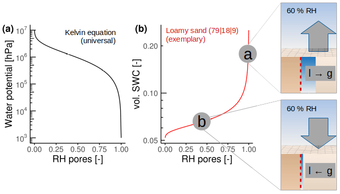
Figure 1Relationship between (a) soil water potential and relative humidity (RH) of the soil pores at 20 °C defined with the Kelvin equation. (b) Illustration of the conversion of water potential from (a) to the respective volumetric soil water content (SWC, m3 m−3) for a loamy sand consisting of 79 % sand, 18 % silt, and 9 % clay, based on the van Genuchten model (van Genuchten, 1980). The representations (labels a and b in panel b) illustrate that at constant atmospheric RH of 60 % at a temperature of 20 °C, the vapor flux direction and phase change (l and g for liquid and gas) within the soil are opposed for different soil water potentials.
3.1 Site descriptions
The study was conducted at the experimental field sites Majadas de Tiétar, Extremadura, Spain (39°56′25.12′′ N, 05°46′28.70′′ E; 260 m a.s.l., ES-LMa*), and Selhausen, Lower Rhine Valley, Germany (50°52′7′′ N, 06°26′58′′ E; about 103 m a.s.l., DE-RuS).
Majadas de Tiétar (ES-LMa*). The field site is a Mediterranean (dry summer) tree–grass ecosystem. The nearest sea is the Atlantic 272 km to the west. The site experiences an average annual temperature of 16.7 °C and receives approximately 650 mm of rain annually over 2004–2022, primarily falling between November and May, followed by extended dry summers (El-Madany et al., 2018). The vegetation at the site is characterized by a sparse tree cover of about 20 %, mainly consisting of Quercus ilex L. with an approximate density of 20 trees ha−1 (Bogdanovich et al., 2021), and pasture understory regularly grazed by cattle. During the growing season, the herbaceous layer dominates, comprising grasses, forbs, and legumes. The fractional cover of these plant forms varies seasonally based on their phenological stage, with important interannual variations influenced by the precipitation seasonal distribution (Perez-Priego et al., 2017). The herbaceous layer typically reaches its peak in late March, with a mean plant area index of up to about 2 m2 m−2; undergoes senescence by the end of May; and regains its greenness in about October (Migliavacca et al., 2017). The soil at the site is classified as an Abruptic Luvisol (Ah, Bt, Btg, C). The upper horizons are characterized according to the USDA classification system as loamy sand (75 % sand, 5 % clay, and 20 % silt) sitting on top of a clay horizon (52 % sand, 18 % clay, and 30 % silt) which starts at a depth of 30 to 100 cm (U.S. Department of Agriculture, 2017; Nair et al., 2019). The regional clay mineralogy was identified as a blend of smectite (45 %), illite (35 %), and chlorite and/or kaolinite (20 %) (NC Geological Survey of Spain (IGME), 1992).
Selhausen (DE-RuS). The agricultural research site, Selhausen, is part of the TERENO-Rur hydrological observatory (Bogena et al., 2018) and contains a lysimeter station and an EC flux tower, which are part of the TERENO-SOILCan lysimeter network in Germany (Pütz et al., 2016) and the Integrated Carbon Observation System (ICOS; Heiskanen et al., 2022). The site consists of 51 agricultural fields (with a total area of 1 km2) representing the heterogeneous rural area in the Lower Rhine Valley. It belongs to the temperate maritime climate zone, with a mean annual temperature of 10.2 °C and with 714 mm of annual precipitation uniformly distributed over the year (Bogena et al., 2018). The site is agriculturally managed with rotating crops (winter wheat, winter barley, winter rye, potato, oat, and catch crops) during the period of investigation, with a winter cereal-only rotation on the lysimeters. As a consequence of the tillage, seeding, and harvest activities, there are large interannual variations in the thickness of the vegetation layer, including prolonged periods of bare soil. The soil at the site is classified as a Cutanic Luvisol (Pütz et al., 2016) and the soil texture of the different soil horizons (Ap, Al-Bv, II-Btv) can be classified according to USDA 2017 as silt loam (U.S. Department of Agriculture, 2017; Groh et al., 2020). The clay mineralogy of the site was identified as a blend, predominantly illite with the presence of chlorite and/or vermiculite and small amounts of kaolinite (Jiang et al., 2014).
Aerial pictures of both sites with the associated footprint climatology of the eddy covariance measurements are shown in Fig. 2.
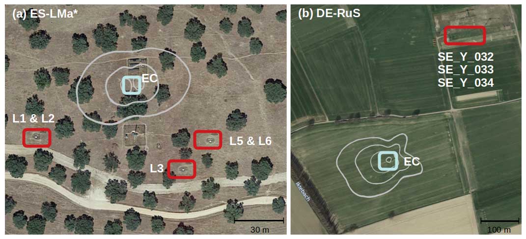
Figure 2Aerial image of (a) the Majadas de Tiétar (ES-LMa*) and (b) the Selhausen agricultural field site (DE-RuS). The squares show the location of eddy covariance (EC) instruments (light blue) and the lysimeters (red) at each site. The EC footprint climatology isolines are overlaid in grey (for 50 %, 70 %, and 80 % of the climatology, respectively; Selhausen: based on ICOS, 2021). Note that the spatial resolution differs (map data from © Google Earth; a – image from Instituto Geográfico Nacional, b – image from GeoBasis-DE / BKG).
3.2 Eddy covariance and lysimeter measurements
At ES-LMa*, the EC system consists of a sonic anemometer (Gill R3-50; Gill Instruments Limited, Lymington, UK) and an enclosed-path IR gas analyzer (LI-7200, LI-COR Biosciences Inc., Lincoln, NE, USA). It is located in an open area at a height of 1.6 m above ground to measure only the fluxes from the sub-canopy herbaceous layer. To avoid confusion with the whole-ecosystem EC system located at 15 m height, we added an asterisk to the site ID. EC raw data were collected at 20 Hz, and flux calculations were performed with EddyPro software (version 6.2.0.). Raw time series were first subjected to de-spiking, and block-average means were then subtracted (Vickers and Mahrt, 1997). Coordinate rotation was performed using the planar fit method for the two primary wind directions (Wilczak et al., 2001), followed by the double-rotation method for the remaining data. Standard integral turbulence characteristics were identified and most problematic records removed (Foken and Wichura, 1996). For more details about the setup and the processing, please refer to Perez-Priego et al. (2017) and El-Madany et al. (2018, 2020). The two dominant wind directions at ES-LMa* are east and west-southwest (Fig. 2a).
In DE-RuS the EC equipment of the DE-RuS station consists of a sonic anemometer (CSAT3, Campbell Scientific, Logan, UT, USA) and an open-path IR gas analyzer (LI-7500, LI-COR Biosciences Inc., Lincoln, NE, USA). The measurement height was 2.34 to 2.55 m above the soil surface near the center of a 9.8 ha crop field. EC raw data were collected at 20 Hz, and flux calculations were performed with TK3.11 (Mauder et al., 2013). Raw time series were first subjected to de-spiking, and block-average means were then subtracted. The planar fit method was performed uniformly across all wind directions. Data points not meeting the assumptions on stationarity and integral turbulence characteristics were removed (Foken and Wichura, 1996). More details about the site, instrumentation, and processing can be found in Ney and Graf (2018). The two software programs used to process the raw data at the two sites (EddyPro and TK3) have been shown to be in good agreement (Fratini and Mauder, 2014).
Two-dimensional footprint analysis aiming to evaluate whether half-hourly flux values are sufficiently representative of the target area was performed for both sites based on the model by Kljun et al. (2015) (illustrated as footprint climatology isolines in Fig. 2; ES-LMa*: 2015–2017; DE-RuS: 2018–2019; more details are given in ICOS, 2021). At ES-LMa* the 80 % footprint climatology is within a distance of 33 m from the tower in the two dominant wind directions. At DE-RuS, 80 % of footprint climatology is within the agricultural field in the dominantly prevailing west-southwest wind direction. λE was converted to water flux (mm) by dividing it by the latent heat of vaporization λ (). The energy imbalance for EC was calculated as the sum of half-hourly turbulent fluxes (H + LE) versus available energy (Rn − G). Note that this leads to an overestimation due to the neglect of storage terms. The full EC time series from ES-LMa* and DE-RuS comprise 8 years of data, with each data set from 1 January 2015 to 31 December 2022.
The lysimeter measurement facility in ES-LMa* consists of three stations in three locations within a distance of 104, 91, and 24 m of each other and with a distance of 66, 56, and 55 m to the EC setup, respectively (Fig. 2a). Each station contains two weighing, high-precision, high-density, polyethylene lysimeters (Umwelt-Geräte-Technik GmbH, Müncheberg, Germany) with a 1 m2 surface area and 1.2 m column height each. The weight of each lysimeter column is measured with three precision shear stress load cells (model 3510, Tedea-Huntleigh, Canoga Park, CA, USA) at a temporal resolution of 1 min. The lysimeters were installed in 2015 by excavating undisturbed soil monoliths from open grassland areas with the natural herbaceous vegetation being preserved. Each station has a lower-boundary control system, consisting of a heat exchange system and porous ceramic bars at the bottom of each column to adjust soil temperature and water content to the conditions of the surrounding soil at the same depth (Groh et al., 2016; Podlasly and Schwärzel, 2013). More details on the technical specifications are given by Paulus et al. (2022) and on the excavation method by Reth et al. (2021). Within each column, SWC and soil temperature (Tsoil, °C) (UMP-1, Umwelt-Geräte-Technik GmbH) are measured at 0.1 m soil depth at a resolution of 0.1 % SWC and 0.02 °C, according to the manufacturer. Heat dissipation sensors, also located at 0.1 m soil depth, additionally provide estimates of Ψm (Tensiomark, ecoTech Umwelt-Messsysteme GmbH, Bonn, Germany). However, it should be noted that the suitability of the heat dissipation method is under debate and this sensor in particular was reported to yield inaccurate readings under dry conditions (Degré et al., 2017; Jackisch et al., 2020). We therefore use the readings only as an indicator of the spatial heterogeneity of Ψm and do not interpret the absolute readings. We calculated RH and vapor pressure of the soil air (esoil, hPa) from Ψm and Tsoil with the Kelvin equation (Edlefsen et al., 1943) (given in Appendix B).
The lysimeter measurement facility in DE-RuS consists of four lysimeter stations, each hosting a set of six weighing lysimeters. The 24 lysimeters were filled with eight different soil types (each soil with three replications); however, for the comparison we use data from three lysimeters that contain the local soil from Selhausen (SE_Y_032, SE_Y_033, and SE_Y_034; https://www.tereno.net/, last access: 14 April 2024) and exclude other soils that are part of the translocation experiment within TERENO-SOILCan (Pütz et al., 2016). The lysimeters in Selhausen are arranged hexagonally (six lysimeters per station), with a distance of about 1.2 m between two adjacent lysimeters. This study comprises data from three weighing high-precision, stainless-steel lysimeter columns (UMS AG, Munich, Germany) (Fig. 2b). Please note that there is a distance of 357 m between lysimeters and the EC setup at DE-RuS, and the agricultural management deviates. The soil texture, however, is the same under and inside the respective measuring instrument. Each column has dimensions of 1 m2 surface area and 1.5 m depth. The weight of each column is measured with three precision shear stress load cells (model 3510, Tedea-Huntleigh, Canoga Park, CA, USA) with a measurement precision of 0.01 kg, like in ES-LMa*. The lysimeters were filled monolithically by the preparative method (Pütz and Groh, 2023), preserving the natural soil structure, and the lysimeter stations were installed in 2010. Pressure at the bottom of the lysimeter was generated by a bi-directional pumping mechanism that allowed either drainage into an external water reservoir (weighted tank) or inflow into the lysimeter from this reservoir, depending on the pressure difference between the lysimeter and the surrounding field soil at 1.4 m depth. Both the pressure head in the field and the bottom of the lysimeter were measured with a tensiometer (TS1, UMS, Munich, Germany). SWC is measured within each lysimeter at a depth of 0.1 m below the surface with time domain reflectometry probes (CS610, Campbell Scientific, North Logan, UT, USA) at a resolution of 0.1 % SWC, according to the manufacturer. More details on the technical specifications of lysimeter facilities within SOILCan are given in Pütz et al. (2016), on excavation methods in Pütz and Groh (2023), and on the Selhausen facility in Groh et al. (2022).
Lysimeter raw weights underwent manual and automatic plausibility checks, and periods with fieldwork/maintenance were removed. The lysimeter raw data were corrected for the pumping activities across the lower-boundary system. To further reduce the impact of noise on the determination of the land surface water fluxes, the adaptive window and adaptive threshold (AWAT) filter routine was applied at both sites. The AWAT filter handles non-stationary measurement errors in the lysimeter raw weight time series (Peters et al., 2014, 2016, 2017). In this three-step process, we employ adaptive techniques to smooth the time series by adjusting the width of the time window for the moving average. Moreover, adaptive threshold values are utilized, considering both the signal strength and noise levels. The evaluation of noise and signal strength is performed by analyzing a moving polynomial and subsequently examining the residuals for each data point. This enables us to accurately determine the presence of noise and the strength of the signal. In the third step, we identify local maxima and minima and incorporate them to prevent slight yet consistent underestimation during changes in the flux direction. This aspect is particularly crucial for the precise detection of minor flux events such as dew or SVA. The details of the AWAT filter are given in Peters et al. (2014, 2016, 2017) and its application to lysimeter raw data in Paulus et al. (2022) for ES-LMa* and Schneider et al. (2021) for DE-RuS.
Based on Paulus et al. (2022), the direction of the lysimeter weight change at each time step (ΔW, mm per unit of time), is used to classify them into one flux category, assuming that there is only one dominant flux during each time step (5 min at ES-LMa* and 1 min at DE-RuS), with
We calculated dew-point temperature (Tdew, °C) from air temperature (Ta, °C) measured at a height of 1 m (Sonntag, 1990). Since the average vegetation height, and hence the level where dew condensation occurs, is at 0.1 m, we estimated °C. This calculation was based on a campaign-based comparison between the Ta sensors at 1 m height and 0.1 m height above the surface (see Paulus et al., 2022, for further details) on soil or plant surfaces (Ts). For ES-LMa*, we additionally chose a last node with the category “residuals”.
The lysimeter time series from Majadas de Tiétar comprises 4 years of data from 1 January 2018 to 31 December 2021. The time series from Selhausen comprises 3 years of data from 1 January 2018 to 31 December 2020. Please note again that at both sites, none of the lysimeters are below the EC stations (see Fig. 2).
3.3 Auxiliary measurements
Additional hydro-meteorological measurements were analyzed at both sites at a temporal resolution of 30 min. At ES-LMa*, meteorological variables monitored were Ta and RH (capacitive humidity sensor CPK1-5, MELA Sensortechnik, Germany), both collected at 1 m height above surface level. Tdew and atmospheric vapor pressure (ea, hPa) were calculated based on Ta and RH (Sonntag, 1990). Precipitation was measured with a weighing rain gauge (TRwS 514 precipitation sensor, MPS systém, Slovakia), and the mole fraction of water vapor in dry air (ρ, mmol mol−1) was measured in a profile of four levels (0.1, 0.5, 1, 2 m) (LI-840 CO2 H2O Analyzer, LI-COR Biosciences Inc., Lincoln, NE, USA).
Shortwave (SW, W m−2) and longwave (LW, W m−2) downwelling (SWIN, LWIN) and upwelling (SWOUT, LWOUT) radiation of the herbaceous layer were observed with a net radiometer (CNR4, Kipp & Zonen, Delft, the Netherlands) at a measurement height of ∼3 m. Ts is calculated from LW, and all equations used for the conversion of meteorological variables are given in Appendix B. Tsoil (Pt100, JUMO, Fulda, Germany) and SWC (ML3, Delta-T Devices Ltd., Burwell, Cambridge, UK) were measured outside the lysimeters at 0.05, 0.10, and 0.2 m depth at a resolution of 0.02 °C for Tsoil and 0.1 % SWC. Phenological shifts of the grass layer in ES-LMa* were examined based on green chromatic coordinates (GCCs) from PhenoCam. For details regarding the camera setup and the computation of this specific vegetation index, we refer to the comprehensive description provided by Luo et al. (2018).
At DE-RuS, Ta and RH were measured at EC sensor height (∼2.5 m, HMP45C, Vaisala, Vantaa, Finland) and precipitation at 1 m with a weighing gauge (Pluvio2 L, OTT, Kempten, Germany). SWIN, SWOUT, LWIN, and LWOUT above the canopy were measured with a net radiometer (NR01, Kipp & Zonen, Delft, the Netherlands) at EC sensor height (∼ 2.5 m). SWC was measured at 0.025 m depth at a resolution of 0.1 % SWC, according to the manufacturer (CS616, Campbell Scientific, Logan, UT, USA). Conversions to other required variables were performed as described above for ES-LMa*.
3.4 Selection of time periods
Since we are particularly interested in the nighttime water fluxes, we compute diel aggregated values (e.g., mean or median conditions, summed flux) from noon to noon (instead of midnight to midnight). Consistent with the classification of fluxes of the lysimeters, we excluded days with rain, fog, and dew formation based on the following criteria: rain = 0, RH < 95 %, and Tdew 0.1 m < Ts. The final selection comprised 641 d in ES-LMa* and 98 d in DE-RuS. Previous observations of SVA in ecosystems occurred after the highest position of the sun, mostly at night. Therefore, we consider phases of different radiation conditions separately. We distinguish between the following periods:
-
day, when the sun is at an angle larger than 6° above the horizon;
-
twilight, from the golden hour (sun at 6° above the horizon) to the end of astronomical twilight (sun at 18° below the horizon);
-
night, between the end of astronomical dusk and the beginning of astronomical dawn;
-
diel, from noon to noon.
We used the function getSunlightTimes from the R software package suncalc (version 0.5.1; Thieurmel and Elmarhraoui, 2022) to determine the time of the day of the respective sun positions based on astronomical algorithms and the coordinates of the field site.
λE fluxes were quality-checked according to Mauder and Foken (2011) and Rebmann et al. (2005), and data with quality flags 0 and 1 were retained for further analysis. As opposed to CO2 fluxes, λE fluxes are not regularly filtered for low-friction-velocity (u*, m s−1) conditions. However, to be conservative we removed the half hours with the u* values below the critical u* threshold (, m s−1) determined using the REddyProc package. To take into account the uncertainty introduced by the u* filtering, we repeated the analysis using the 5th and 95th percentiles ( and ) of the estimate (Papale et al., 2006; Wutzler et al., 2018; given in Appendix Table F1).
For each lysimeter and half hour, the number of SVA observations was counted individually. If during the half hour at least 20 min was classified as SVA, the half hour was counted as SVA-dominated (individual column). Since days with dew, fog, and rain were filtered out, the remaining (non-SVA) 10 min can only contain evaporation measurements. Then, for each half hour, we counted the number of lysimeters that detected SVA.
3.5 Comparing downward water fluxes detected with lysimeters and eddy covariance measurements
We will use F (mm per unit of time) to represent water fluxes measured by the respective measurement method where flux direction is indicated in the subscript. Thus, FOUT,EC and FOUT,LYS indicate evaporation, whereas FIN,EC denotes negative (i.e., downwardly directed) λE fluxes and FIN,LYS denotes positive lysimeter weight changes, classified as SVA observations.
We investigated (i) the temporal consistency of the FIN between methods and (ii) the magnitude and comparability of the measured FIN totals. To assess (i) temporal consistency, we count whether and how many weighing lysimeters detect FIN,LYS at the time of the occurrence of FIN,EC. We compute precision and recall metrics (given in Appendix B). To examine the concurrence among instruments concerning the seasonal onset of SVA-dominated nights, we identified the first period each year during which 5 consecutive days exhibited more than 4 h of FIN. At the diel scale, we compared the timing of the first and the last observation of FIN for each night. To compare (ii) the magnitude of the flux totals, we compare the half-hourly mean absolute error (MAE, mm per half hour) between the lysimeter median and the EC measured value (i.e., different methods, different vertical and horizontal locations), as well as between the individual lysimeter columns (i.e., same method, different horizontal locations).
Since the measurement location of the two methods is located at a vertical separation about 2 m from each other, a temporal shift and an attenuation of the signal are possible. Therefore, in addition to half-hourly measurements, we also compare the diel sums between techniques for different subsets of the data: (a) all night (quality-filtered) fluxes F, (b) all (u* and quality-filtered) FIN,EC fluxes, and (c) all (u* and quality-filtered) FIN,EC fluxes during simultaneous FIN,LYS across all lysimeters. For the comparison, we use the Pearson correlation coefficient (R), MAE, coefficient of determination (r2), and root mean square error (RMSE, mm per unit of time). Additionally, we compare the slope and the intercept using major-axis regression () (MA), which was performed with the R package lmodel2 to take into account the fact that the uncertainties on the y and x axes are comparable (Legendre, 2018).
Heterogeneous vegetation structures create micro-meteorological differences, which in turn affect F. To assess whether the differences between the EC and lysimeters (ΔLYS,EC) in ES-LMa* can be better explained by variations in micro-meteorological factors or by variations in the soil hydraulic conditions, we used a feature selection model with ΔLYS,EC as the dependent variable (Jung and Zscheischler, 2013) and the predictors given in Appendix C. The list of given predictor variables can be grouped into four distinct categories: meteorological conditions, the uncertainty in the EC technique, soil conditions, and heterogeneity across lysimeters. Note that the structure of the underlying data causes differences in the information content between the variable categories. Heterogeneity across lysimeters incorporates spatiotemporal information, while all other categories only contain temporal information. Due to gaps in the lysimeter auxiliary measurements, the year 2018 was excluded from this part of the analysis.
The advantage of the feature selection method is that it is suitable for distinguishing the importance of individual features although there is a high correlation within the set of given features, which is the case for many soil hydro-meteorological features. Feature selection was performed using random forest (Breiman, 2001) as a first modeling step (100 trees) on a subset of predictor variables and using the out-of-bag estimate to calculate the cost function. Then, an ensemble of equally good models was selected (all models with mean squared error (MSE) > min(MSE) + 1 SD(MSE)) accounting for the performance differences based on the stochasticity of the random forest method. To explain the effects of individual predictors identified with the feature importance on ΔLYS,EC, we used Shapley additive explanations (SHAP) values (Lundberg and Lee, 2017). SHAP values were calculated on the unseen test data in a 10-fold cross-validation. We tested two model versions with model.v1, only providing spatiotemporal variables, and model.v2, additionally providing the lysimeter ID as a categorical input variable. Potential SWC-related thresholds in the diel relationship between SVA and evaporation were assessed by employing piecewise linear regression. The threshold is defined as the breaking point between two linear models fitted separately to the data obtained from the EC and the lysimeter to test if these thresholds are consistent across the two methods.
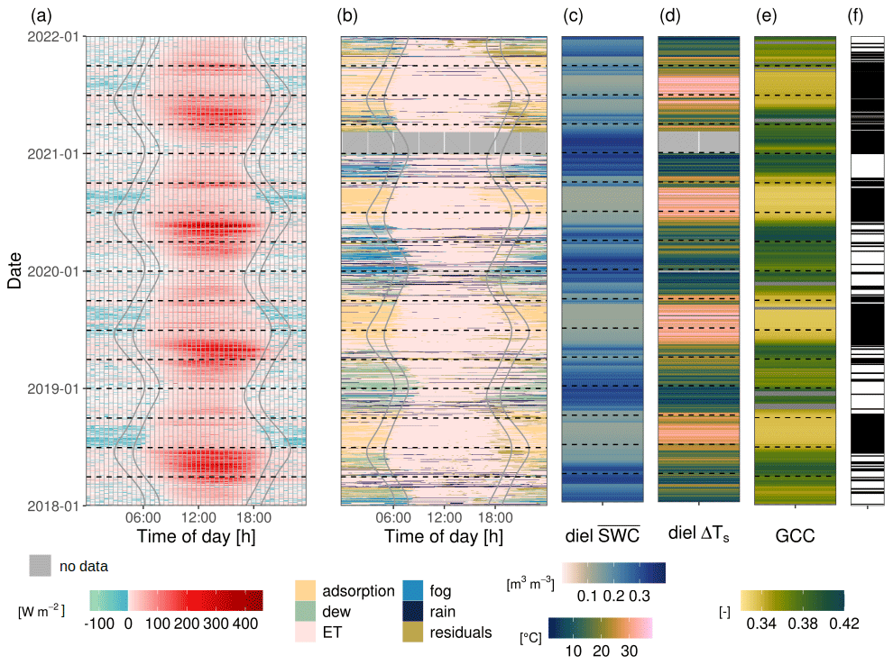
Figure 3Diel and seasonal dynamics of (a) quality-filtered latent heat fluxes from the eddy covariance method and (b) dominant lysimeter fluxes (exemplarily shown for L6) at the Majadas de Tiétar field site. Solid vertical lines mark the end of the night, sunrise, sunset, and the beginning of the night, respectively (determined with the geographic coordinates of the field site). Panel (c) shows diel means of volumetric soil water content at 0.1 m depth (diel ) and (d) maximum diel difference in surface temperature (Δ Ts). Green chromatic coordinate (GCC) values for the grasses are shown in panel (e). In panel (f) the dates selected for this comparison based on the absence of rain, fog, and dew are marked as horizontal black lines (see Sect. 3.4).
4.1 Seasonal and diel meteorology
In the semi-arid site ES-LMa*, the FEC fluxes follow a pronounced seasonal cycle (Fig. 3a; for abbreviations see Table A1). The largest FOUT,EC fluxes occur every year between March and June. During this period, (i) soil water supply is high as soil moisture is replenished after winter and (ii) soil water demand is also high as sufficient energy is available for evaporation and vegetation is active (Fig. 3c, e). Each year around the end of May, SWC declines sharply in response to reduced precipitation (Fig. 3b, c). Consequently, evaporation is reduced, leading to lower RH and consequently an increase in atmospheric demand. Within a couple of days, greenness decreases, indicating the withering of the grasses, while the diel amplitude of Ts increases (Fig. 3a, d, e).
When SWC is high, F oscillates around zero between sunset and sunrise. In contrast, when soil is dry, a nighttime FIN,EC emerges shortly after the daytime evaporation declines (Fig. 3a). This pattern is most obvious in the second half of the night. This observation was confirmed by the lysimeter records across all 4 years of observations: nighttime weight increases during this period occurred between sunset and sunrise and were classified as SVA (Fig. 3b). An illustration of the daily measurements from both instruments over 4 d of the dry season is shown in Appendix Fig. D1. It shows that RH remains below 70 % and Ts never reaches Tdew, which confirms that the FIN is not related to fog deposition or dew formation.
The seasonal cycles of FEC in the temperate site DE-RuS are different from ES-LMa*. Here, the annual period of active daytime FOUT,EC lasts longer, i.e., from February until November (Fig. 4a). Strong changes in FOUT,EC during summer are related to crop management (Fig. 4a, e), revealing substantial differences in 2019 compared to 2018 and 2020. While in 2019, FOUT,EC is consistently high over the whole summer, in 2018 and 2020 it is sharply reduced in July, associated with the harvest of the crops (Fig. 4a, e). Similarly to ES-LMa*, this reduction is followed by several weeks of increased diel Ts difference, reaching values of more than 30 °C between the day and night in bare-soil conditions with harvest residuals in the EC source area (Fig. 4d). In contrast, in the summer of 2019 such extreme Ts differences only occurred on individual days, likely because the soil was wet enough near the surface to keep bare-soil evaporation close to potential evaporation. The nighttime fluxes in DE-RuS oscillate around zero in wet conditions, but as opposed to ES-LMa* this is also the case in dry conditions. The lysimeter records confirm that in DE-RuS, less frequent FIN during the night occurs compared to ES-LMa* in all seasons. Lysimeter weight increases are only sporadic during individual days and a short number of hours classified as SVA. The only exception is a period of 2 weeks in 2018 right after the harvest.
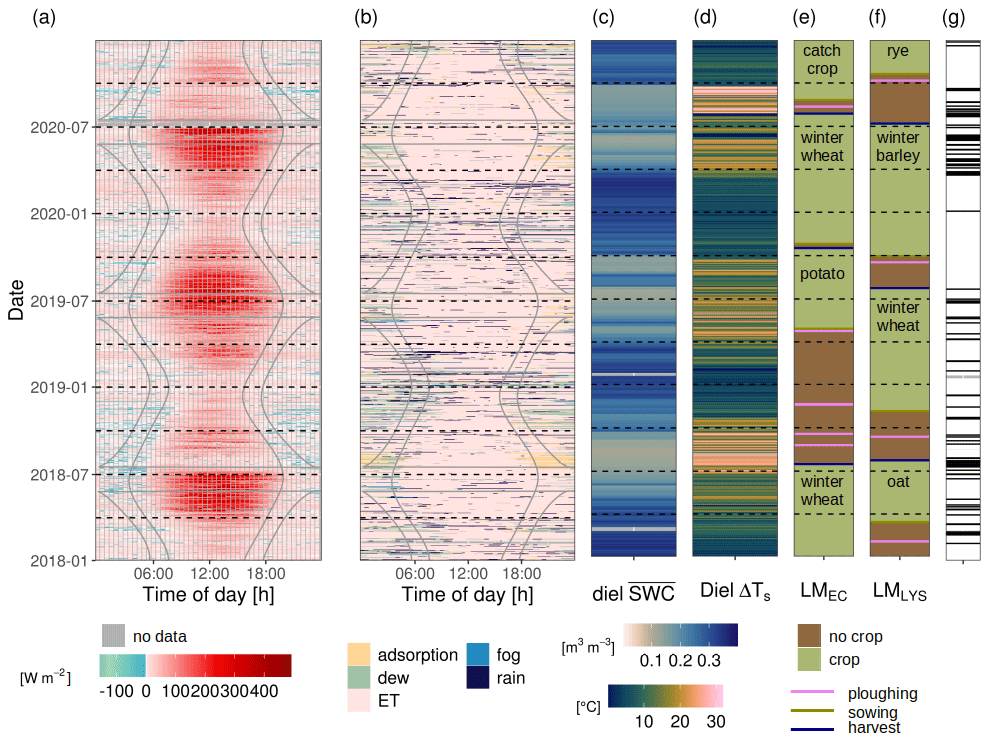
Figure 4Diel and seasonal dynamics of (a) quality-filtered latent heat fluxes from the eddy covariance (EC) technique and (b) classified dominant lysimeter (LYS) fluxes (exemplarily shown for Se_Y_032) at the Selhausen agricultural field site. Solid vertical curves mark the end of the night, sunrise, sunset, and the beginning of the night, respectively (determined by the geographic coordinates of the field site). The mean volumetric soil water content at 0.1 m depth and maximum diel difference in surface temperature (ΔTs) are displayed as diel measurements in panels (c) and (d). Land management (LM) is illustrated separately below the EC (e) and on the LYS (f). In panel (g) the dates selected for this comparison based on the absence of rain, fog, and dew are marked as horizontal black lines (see Sect. 3.4).
The different conditions in the two ecosystems and the fluxes associated with the lysimeter weight changes confirm that, while SVA is a frequent flux in ES-LMa* across the years, it occurs only occasionally in the temperate agricultural ecosystem. The patterns in the EC observations also support these findings.
These results show that SVA in DE-RuS only occurred during a few weeks in the year 2018. In this time period (20 July 2018 until 22 August 2018) the Standardized Precipitation Evaporation Index (aggregated over 30 d; SPEI_30) at DE-RuS indicates extreme drought (Appendix Fig. E1; Svoboda et al., 2002) (Pohl et al., 2023, 2022). Such dry conditions during annually more than 2 weeks have been recorded at this site only five times since 1950. However, out of these five times, three occurred after 2010 (2011, 2018, 2020) (Pohl et al., 2022). The results from the temperate ecosystem confirm statements from the classic literature that SVA is strongest in central-European climate conditions in late summer when the soil is dry and uncovered (Blume et al., 2016b). At ES-LMa*, in contrast, SVA was observed each summer, but the years of investigation contained “only” moderate and severely dry periods (Appendix Fig. E1a), suggesting SVA to be the norm in the semi-arid area. This indicates that under the current climate, SVA in temperate (agricultural) ecosystems only occurs during extremely dry conditions with no, or only little, vegetation. It underscores that while the probability of occurrence of SVA is influenced by climate (i.e., more common in semi-arid and arid regions), it can also occur in more humid regions. This is because it depends on soil-intrinsic physical properties, such as texture (clay content, clay mineralogy, and organic carbon content) (Orchiston, 1954; Arthur et al., 2019; Yukselen-Aksoy and Kaya, 2010) or soil structure that affects vapor transport characteristics (i.e., soil diffusion coefficient), and it can happen anywhere if the dynamic requirements like temperature and moisture gradients are met. Considering the current climate change and increase in aridity foreseen in models, the importance of SVA might also become more prominent in temperate ecosystems.
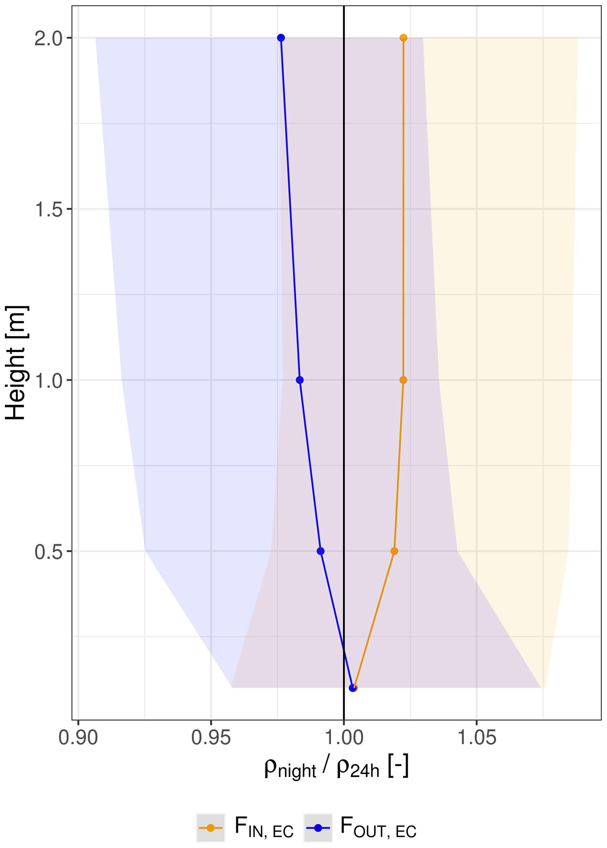
Figure 5Vertical profile of mean nighttime absolute humidity (ρnight) divided by the mean diel absolute humidity (ρ24 h) across all heights. The points and shaded areas illustrate the median and inter-quartile range during moments at night with FOUT,EC in blue and FIN,EC in yellow.
The vertical gradient of ρ between 0.1 and 2 m height above the soil during nights in ES-LMa* was investigated separately for conditions of FOUT,EC and FIN,EC, relative to the diel mean ρ (Fig. 5). During the occurrence of FOUT,EC, the air is relatively dry compared to the 24 h mean but wetter towards the soil surface. During the occurrence of FIN,EC, it is the opposite situation, with the air at 2 m height being relatively moist but dry towards the soil surface. These measurements independently indicate that under conditions of FOUT,EC, the air close to the soil is wetter than the atmosphere, whereas under conditions of FIN,EC it is drier. From a gradient perspective, the latter case creates a vapor flux towards the soil, as described in the theoretical example in Sect. 2 and Fig. 1. The measurements also indicate that FIN,EC fluxes are predominantly related to processes happening at the soil surface and to a lesser extent to the subsidence of dry air masses from the higher atmosphere because the profile between 1 and 2 m height is stable. Since the distinction between the micro-meteorological conditions shown in Fig. 5 is based only on observations of EC, this result (based on ρ as an independent observation) supports our hypothesis (ii) that EC can detect SVA.
4.2 Temporal patterns in the flux direction: consistency among instruments
We compared the flux directions measured with both instruments to investigate the consistency between measurement methods. The results are summarized in Table 2. At ES-LMa*, 4017 half hours of FIN,EC were observed on 448 d, which is 30 % of the total measurement period. During 67 % of these EC observations, three or more (> 50 %) of the lysimeters measured SVA. During 88.5 % of the measured FIN,EC fluxes, at least one of the lysimeters measured SVA simultaneously. Applying the value to filter out non-turbulent conditions removes 56 % of the half-hourly measurements. The agreement between measurement methods after u* filtering differs only marginally, which is consistent across different values (see Appendix Table F2). Excluding daytime and twilight increased the relative agreement with lysimeters by 6 %.
Between 89 % and 71 % (depending on the number of lysimeters considered) of all measured FIN,EC fluxes (before u* filtering) are in agreement with FIN,LYS as the reference ground truth (precision). Of all FIN,LYS fluxes, however, only 53 % are detected by the EC instrument (recall). The recall rate increases to 75 % when all lysimeters are in agreement on the flux direction. These results suggest that in ES-LMa*, the great majority of FIN,EC fluxes are signals of SVA and that the EC method tends to underestimate the number of half hours with FIN detected by lysimeters by at least 25 %. This could be partly related to a strong spatial heterogeneity of SVA, with EC performing best when SVA occurs across the field site and not only in a few locations.
This can be related, on the one hand, to the high spatial variability in the soil conditions and, in some cases, the conditions at a lysimeter location not being representative of the whole ecosystem and, on the other hand, to the variability in the source area of the fluxes measured by eddy covariance (eddy covariance footprint), whose shape and orientation depend on the wind direction and turbulence conditions, the first of which is highly dynamic in ES-LMa* (see El-Madany et al., 2018). Although the lysimeters were placed in an area representative of the ES-LMa* footprint, they were not placed in the immediate vicinity of the EC instruments to avoid disturbances. Therefore, we expect a better agreement between lysimeters and EC data only when all lysimeters agree in SVA detection, and thus when the process occurs in many locations on the site and is therefore more likely to be detected by the EC independently of the shape and orientation of the footprint area.
Table 1Comparison of the number of simultaneous observations of flux direction towards/into the soil between EC and lysimeters for different filter criteria for ES-LMa* and DE-RuS.
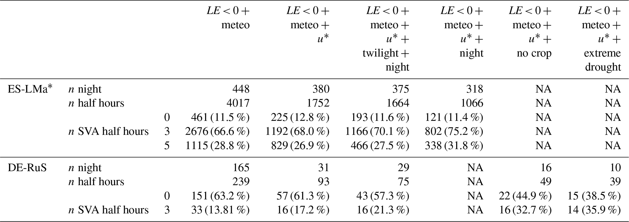
NA: not available.
In DE-RuS, 239 half hours of FIN,EC was observed on 165 d, which is 15 % of the measurement period. In contrast to ES-LMa*, for 63 % of the FIN,EC half hours, no SVA was detected by the lysimeters. Filtering with the and for phases of twilight or night slightly decreased the number of hours matching lysimeter SVA; this could however also be an effect of the reduction in the sample size, which amounts to 40 % after u* filtering. The agreement between methods increased under conditions of bare soil and extreme drought despite a strong reduction in the sample size to only 16 and 10 d, respectively. The highest agreement was found for conditions of extreme drought, but even then, 39 % of the FIN,EC fluxes were not accompanied by lysimeter SVA. Under such conditions, only 39 half hours from 10 d was available for comparison.
One potential reason for this difference between the sites is different crop and crop residue management in DE-RuS, since the height of the vegetation influences gas exchange. SVA was reported to be reduced below or in the vicinity of tall, active vegetation by 76 % (Kosmas et al., 2001). Also the larger distance between the instruments in De-RuS (357 m), as compared to ES-LMa*, could have an effect on the results. Another reason could be that the topsoil in DE-RuS remains relatively wet as compared to ES-LMa*, with a mean and standard deviation of SWC amounting to 16.8 ± 6.6 % and 7.8 ± 4.8 %, respectively. DE-RuS remained much wetter than the semi-arid site even under extreme drought (13.1 ± 2.2 %). At the same SWC under controlled conditions, the soil from DE-RuS should theoretically have a similar or higher capacity to adsorb water compared to the soil in ES-LMa* due to its high clay content (17 % compared to 5 %), which influences the water sorption behavior more strongly than the mineralogy for mixed soils with low kaolinite content (Arthur et al., 2015). Hence, these effects of the soil properties do not come into play when the overall climatic conditions are too wet.
The results support our hypothesis (i) that the EC method is able to capture the difference between the two sites in different climates, detecting far fewer half hours of FIN,EC at the temperate site. Since more data are available for the statistical comparison of FIN between methods from ES-LMa*, compared to DE-RuS, we will predominantly concentrate on the methodological comparison based on data from ES-LMa*.
The timing of the first observation of FIN,EC at the diel scale is consistent between years in ES-LMa*. Usually, F turns negative within the hour around sunset or later during the night (Figs. 3a and G1a). The last observation of FIN,EC is usually around sunrise (Fig. G1b). However, there is a stronger delay observable in the morning, indicating FIN,EC fluxes often continue in the first hour after sunrise. An explanation for this observation could be the shallow angle of the sun right after sunset, delaying surface heating until it reaches a higher position in the sky. At the seasonal scale, we compared the agreement between methods by defining the onset of prolonged FIN as more than 4 h during at least 5 consecutive days. In ES-LMa*, the lysimeters consistently detect this onset earlier during the years, compared to EC (Appendix Fig. G2). In 2018 and 2019, the time difference was less than 2 weeks (13 and 9 d, respectively). But in 2020 it amounted to 1 month, and in 2021 nearly 2 months (32 and 58 d, respectively). In 2020, the EC also had already detected prolonged FIN,EC earlier in the year, although only over the span of 3 consecutive days, highlighting that the definition of the onset of prolonged SVA strongly affects these results. Nevertheless, when considering the prospective benefits of these outcomes, we believe that a definition that ensures a more cautious assessment, as opposed to an overestimation, is preferable. A potential explanation for the mismatch between methods in these 2 years is frequent rain events during the dry-down phase in 2020 and 2021, as compared to 2018 and 2019, causing the flux amount to be below the limit of detection of the EC method but not the lysimeter, as will be demonstrated in the next section.
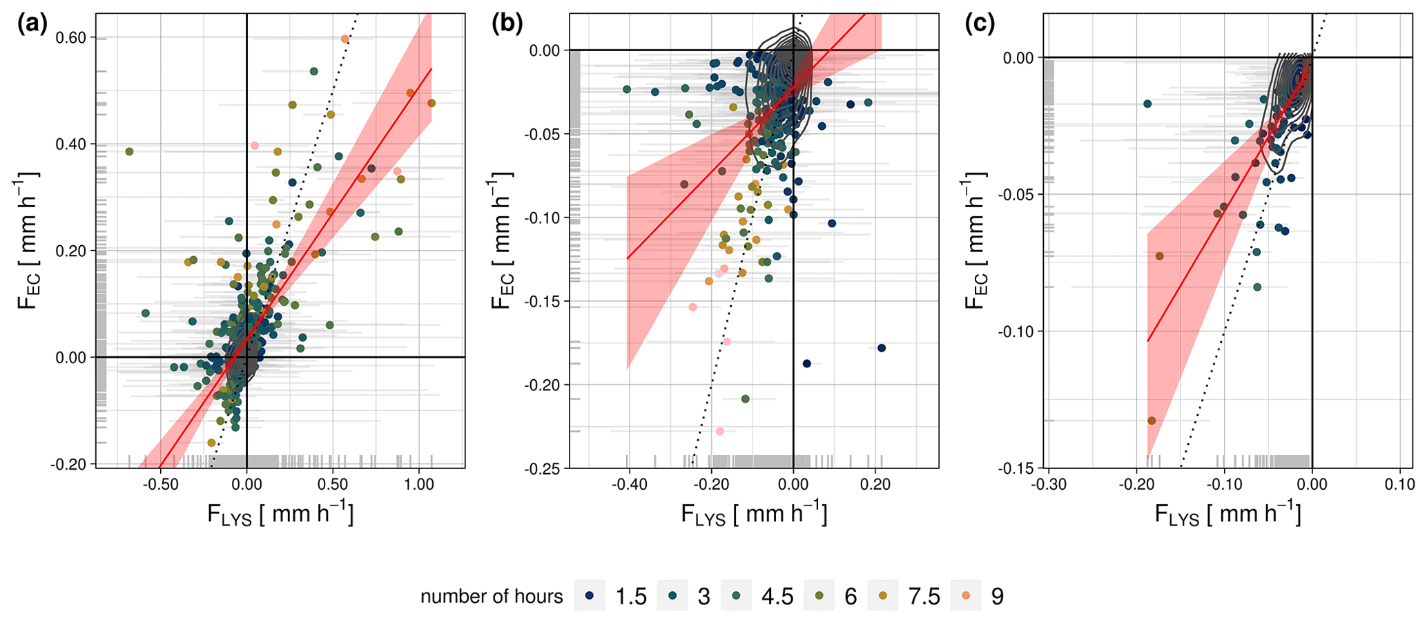
Figure 6Comparison between nighttime sums of lysimeter-measured water fluxes (FLYS) and eddy-covariance-measured fluxes (FEC) in Majadas de Tiétar (ES-LMa*) for different subsets of the data: (a) all good-quality nighttime fluxes, (b) negative EC nighttime fluxes, and (c) negative nighttime fluxes and all lysimeter fluxes classified as soil adsorption of atmospheric water vapor. The red line illustrates a major-axis-regression model and the red shading the confidence interval of the model. The dotted black line illustrates identity. Horizontal grey lines illustrate the minimum and maximum sum observed from single lysimeter columns. The color code illustrates the number of hours over which this sum was formed. This depends on how many observations were measured for the respective conditions on each night.
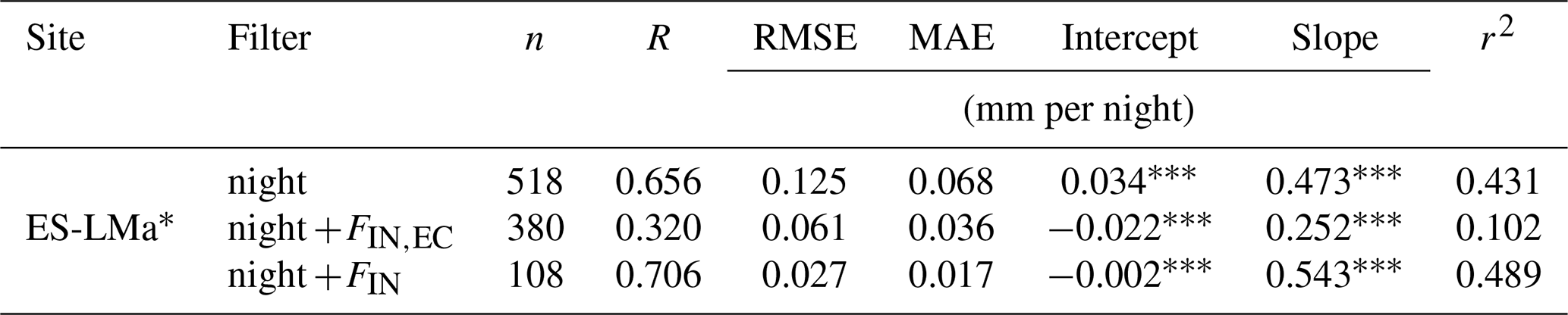
Table 2Statistics for the comparison of FIN,EC and FIN,LYS as nighttime sums in ES-LMa* with different filtering periods. See also Fig. 6.
* Asterisks represent significance level with * p≤0.05, p≤0.01, p≤0.001.
4.3 Amounts of soil water vapor adsorption quantified by eddy covariance and lysimeter measurements
The comparison between the integrated nighttime F sums is illustrated in Fig. 6, and the respective statistical summary is given in Table 2. In ES-LMa* we find that r2 and slope, which describe the relationship between the mean lysimeter-measured flux magnitudes and the EC-measured flux magnitudes, are similar for the case where all good-quality u*-filtered nighttime measurements are compared, including FOUT and FIN (Fig. 6a) or only FIN (Fig. 6c) (r2 of 0.431 and 0.495 and slopes of 0.473 and 0.543). This indicates that generally there is a strong dampening in the signal recorded by the EC method compared to the lysimeters but no systematic bias in the good-quality nighttime FIN,EC compared to the nighttime FOUT,EC.
The strong dampening of the signal is only observed in ES-LMa*. In DE-RuS, there is generally a better agreement between lysimeter and EC fluxes, expressed by a strong correlation (0.858) when all good-quality nighttime fluxes are considered (Appendix Fig. H1 and Table H1). However, the limitation in observation data (n=6) does not enable us to draw any conclusions about the consistency of the pattern in DE-RuS when considering FIN only.
The EC method consistently underestimates F at ES-LMa* compared to the lysimeters, but there is also a great variation between individual lysimeters (grey bars in Figs. 6 and I1). Lysimeter L3, L5, and L6 and the EC method seem to have a much better linear relationship compared to lysimeter L1 and lysimeter L2, indicated by the scatterplot showing a straight line close to the identity line. However, we find higher agreement between EC and the median across the lysimeters (Table 2) than between EC and individual lysimeters (Table I1). One interpretation of this result could be that each lysimeter covers a smaller spatial scale (1 m2 each) compared to the EC (illustrated in Fig. 2 as footprint climatology) but the average across lysimeters better represents the spatial mean and is therefore more in line with the EC observations.
Nevertheless, a systematic difference between the measuring instruments in the form of a bias remains. We evaluated the difference for different values (see Appendix Table F3). When considering only measurements above , the strength of the correlation increases to 0.79 and bias decreases to 0.028 compared to the median . Choosing a low of 0.01 m s−1 increases the mismatch compared to the median . This is not surprising as under stable nighttime conditions the ratio between vertical and non-vertical (drainage and advection) movement of F is expected to be smaller. As a result, a larger proportion of the total F leaves the source area undetected by the EC sensor than in daytime measurements with good atmospheric mixing (Wohlfahrt et al., 2005). Therefore, as in the case of CO2 fluxes, we can expect an underestimation of λE fluxes under low-u* conditions, leading to the observed systematic differences, which are partially relieved when a more conservative (higher quantile of the distribution) is used.
It is important to note that our results are based on negative λE observations only. Considering the low fluxes at night and the random uncertainty in the EC data (Hollinger and Richardson, 2005; Lasslop et al., 2008), we could bias the fluxes by removing values that are close to zero or slightly positive. We would like to disprove the hypothesis that the relationship between the lysimeter and EC observations is based only on the bias introduced by the random error in the EC with three details from our results: (1) all integrated flux sums (except one, on 12 August 2020) are more negative than the error propagation of the random error associated with each half-hourly EC measurement (illustrated in Fig. J1). (2) If the FIN,EC were mainly the sum of the negative fraction of the random noise, it should not be linearly related to FIN,LYS when the sum is calculated over the same length of hours. We find, however, that the linear relationship between FIN,EC and FIN,LYS is weak when considering only short time periods (i.e., 1 h, R=0.05) and strong when considering longer time periods (i.e., 4 h, R=0.6). This indicates that for continuous measurements of FIN,EC, a substantial part cannot be (solely) explained by noise. (3) We find consistent strength in the statistical measures – irrespective of comparing all nighttime fluxes F or only nighttime FIN fluxes (when we assume as a community that good-quality nighttime FOUT,EC fluxes are valid observations, as is already the base of published work, i.e., of Padrón et al., 2020, or Han et al., 2021).
Although in this study we are dominantly interested in the differences in FIN, the drivers of the fluxes and causes of the mismatch are the same as for FOUT. Generally, the flux loss of EC has been acknowledged numerous times (Massman and Lee, 2002), often expressed in a non-closure of the energy balance (Foken, 2008; Mauder et al., 2020) and in a smaller magnitude measured by EC as compared to lysimeters. In a former study in ES-LMa* FOUT,EC amounted to 35 % less compared to FOUT,LYS (Perez-Priego et al., 2017). This finding was independent of the spectral correction method for the EC (i.e., analytical – Moncrieff et al., 1997 – or in situ – Fratini et al., 2012). They suggested that the mismatch in dry periods in ES-LMa* could potentially be explained by strong radiation gradients due to the shade cast by the trees causing flux divergences. At a temperate site in the Prealps, the underestimation of lysimeter evaporation with EC was 30 % (Mauder et al., 2018). Florentin and Agam (2017) reported from an arid desert with homogeneous surface conditions that nearly 50 % of the lysimeter fluxes were detected with EC for both FOUT and FIN. Although a definitive explanation could not be reached for the arid site, at the temperate site, the dissimilarity between the instruments was primarily attributed to the absence of energy balance closure in the EC system. Since there is a large variation in agreement between individual lysimeter stations in ES-LMa*, we investigate the amount and potential drivers of the mismatch in the following section (Sect. 4.4).
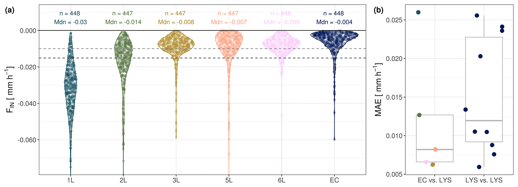
Figure 7(a) Distributions of half-hourly readings shown individually for each lysimeter and the EC in Majadas de Tiétar. Only periods during which adsorption and negative latent heat flux were measured uniformly were selected. The horizontal dashed lines show the mean (black) and median (grey). (b) Mean average error (MAE, mm) between individual lysimeter columns and EC (between techniques) and MAE between lysimeter columns (same technique).
4.4 Identification of the variables influencing the difference between lysimeters and EC SVA measurements
Figure 7a illustrates the distributions of half-hourly values of FIN for each individual lysimeter column and the EC instrument in ES-LMa*. The median of EC observations is lower than the median across all observations from individual lysimeters (−0.004 mm h−1; median-Lys). However, there is also a large range in the observations across individual lysimeters, revealing that the MAE between lysimeters is larger than between the two measurement techniques (Fig. 7b). A larger mismatch exists between EC and observations from station 1 (L1 and L2) compared to the other two stations. We investigated the potential reasons for the mismatch between the two instruments by means of a predictor variable selection procedure based on a random forest model analysis with the deviation between EC and lysimeter as the dependent variable (Jung and Zscheischler, 2013). Figure 8a shows an estimate of variable importance based on how often each predictor variable was selected in the best models for model.v1. The four most frequently chosen variables were lysimeter SWC, ea, Ts, and Ψm. Out of the 16 selected variables, 7 are related to soil temporal and 6 to soil spatiotemporal variability (soil variables measured in the lysimeter columns). These two groups of variables also have an overall stronger impact on the prediction (Fig. 8b) as compared to variables related to the temporal variability in atmospheric state or related to the uncertainty in the EC technique.
The primary factor influencing the variation between instruments is SWC within the lysimeters. The deviation between instruments decreases at lower SWC (Fig. 8c) and higher Ts (Fig. 8d). The fraction of variance explained by the random forest model is 0.449 according to the out-of-bag (OOB) score. In our analysis, this value is acceptable, since we use it in an explanatory context and not for prediction, knowing that part of the variation between the two instruments is random noise. Interestingly, the model performance also does not substantially improve when the lysimeter ID is provided as an input variable (model.v2), supporting the relevance of the SWC within columns as main explanatory variable (r2 = 0.449 and 0.438, RMSE = 0.009 and 0.009 mm h−1, MAE = 0.004 and 0.004 mm h−1). Although the lysimeter ID is selected as a static predictor variable (see Appendix Fig. K1), the dynamics of soil moisture and temperature within lysimeters are more important to explain the observed difference between lysimeter and EC. This means that the lumped effect of static properties which might deviate between lysimeters such as clay or organic matter carries less information content for the prediction of the differences between instruments. Based on these results, it can be inferred that approximately 45 % of the discrepancy in FIN between the lysimeter and EC in ES-LMa* is dominantly influenced by the spatiotemporal variability in soil moisture and temporal variability in surface temperature.
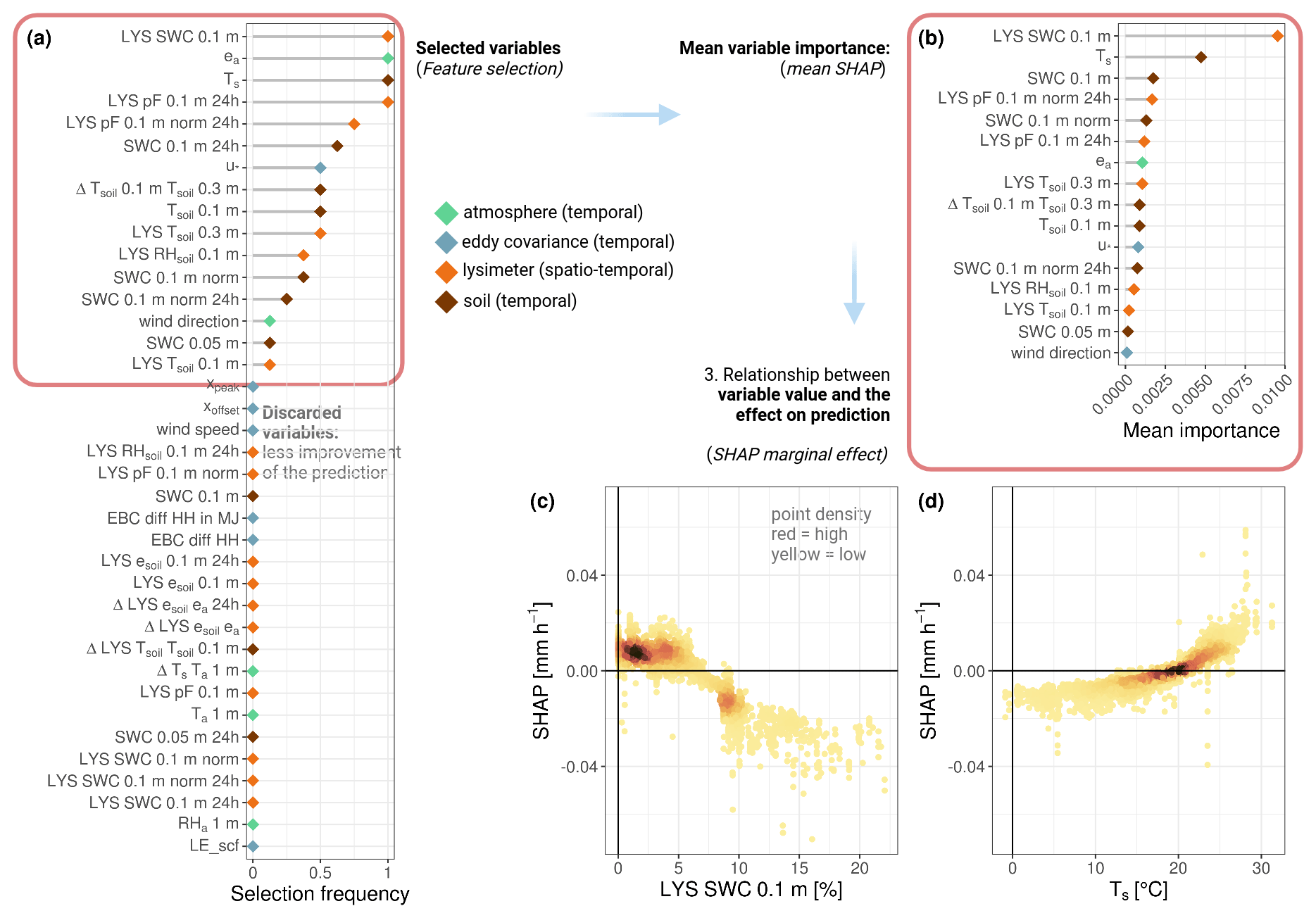
Figure 8Panel (a) depicts the selection frequency of the predictor variables of the best models from the first round of the feature selection procedure. The selected variables (indicated by the red rectangle) were subsequently incorporated in a model ensemble, and their mean importance for the prediction is presented in panel (b). Panels (c) and (d) display the marginal effects of the two most influential predictors, respectively. The full form and explanation of all variables are given in Table C1.
Our finding that SWC and Ts are ranked as the most important variables (based on their mean SHAP value) to explain the deviation between instruments is in line with SVA theory and other field observations. SWC and Ts are both drivers of SVA, controlling the strength of water retention as well as the vapor flux velocity. Several experimental studies confirmed small-scale variation in adsorption quantities of up to 100 % within a 4 m distance only due to soil exposure and the influence of the vegetation canopy (Verhoef et al., 2006; Kidron and Starinsky, 2019), and numerical models show that under dry conditions, diel temperature oscillations are substantial drivers of SVA (Saaltink et al., 2020). Here Fig. K1b and c show that the FIN amount increases with lower lysimeter SWC and higher Ts and, under these moments, the discrepancy between the instruments is reduced. One explanation for this effect could be a larger signal-to-noise ratio. Another explanation might be a higher spatial variability in SWC for medium compared to dry conditions (Vereecken et al., 2007). Since Spanish tree–grass ecosystems (dehesa systems) have a savanna-like structure, they are known to have very heterogeneous and patchy surface conditions, which propagates into the surface energy and water balance, due to the heterogeneous vegetation cover and fertility islands below and around the tree canopies that have very different conditions in terms of soil properties compared to the open grasslands. It is therefore possible that soil heterogeneity conceals the effect of variables associated with EC uncertainty in the mismatch, which should be checked in a more homogeneous ecosystem. This is supported by the detectable effect of the u* that shows that the discrepancy between instruments decreases with higher u* (see Fig. L1), but its effect on the mismatch is 1 order of magnitude smaller than the effect of lysimeter SWC and Ts.
Note that variables measured within the lysimeters carry additional spatial information content compared to the other variables, and hence their importance might be inflated. However, this is not the case for the soil-related variables, which still contribute substantially more compared to the EC uncertainty-related variables, suggesting that our conclusion that soil-related variables are more important than EC uncertainty-related variables is robust. It is further possible that the spatiotemporal differences in soil hydraulic conditions of the lysimeters are caused by small differences in soil properties such as clay or soil organic carbon content. Both variables are known to substantially increase soil sorption capacity and to generally affect soil water retention characteristics (Arthur et al., 2015, 2016). At the Majadas field site, the topsoil clay content is relatively constant between 0 % and 5 %, but an individual topsoil sample from outside the lysimeters contained 18 % clay. Such outliers in the spatial distribution of clay content have substantial non-linear effects on small-scale variations in soil water retention characteristics at the dry end of the water retention curve and thereby could cause the observed variability in SWC between lysimeters.
These results only reflect potential drivers of the differences between the two instruments during the times when SVA occurs, meaning that the model only receives input data from a very specific, filtered period of time. The drivers of the differences in FOUT are (potentially) different but are outside the scope of this analysis. Additional reasons for mismatch can be related to advection, non-closure of the energy balance, changes in the source area (extension and position of the flux footprint), or island effects of the lysimeters.
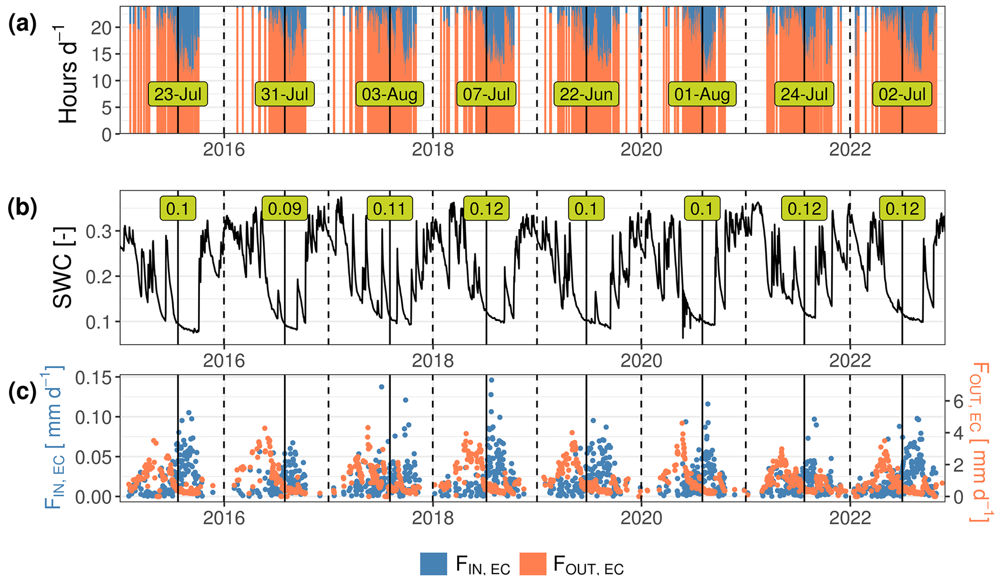
Figure 9Panel (a) illustrates the diel fraction of positive (red, FOUT,EC) and negative (blue, FIN,EC) λE fluxes measured with EC. The dashed vertical lines mark the onset of adsorption-dominated nights in ES-LMa*, defined as the first periods each year, where 5 consecutive days with more than 4 h each of FIN was observed. The annotation in (a) gives the respective day for each year, with the respective soil water content (SWC) at 0.05 m depth given in panel (b). In panel (c) the evolution of the diel FIN,EC and FOUT,EC are presented as weekly means. In all panels, the solid vertical curves illustrate the threshold and the dashed vertical lines illustrate the beginning of the next year.
4.5 Implications of soil water vapor adsorption for the soil water balance
In the previous sections, we demonstrated that FIN,EC fluxes under the selected conditions at our semi-arid site ES-LMa* carry a meaningful signal of SVA. In the last section of this paper, we would like to build on these results and use the new opportunity to (i) investigate the onset of SVA in ES-LMa* over a longer period of time with EC only and (ii) investigate the importance of SVA for the diel soil water balance.
We investigate the onset of prolonged SVA determined based on EC observations in ES-LMa* for each dry season between 2015 and 2022 based on the hours per day of FIN,EC in Fig. 9. The long-term data reveal the onset varying in time between 22 June 2019 and 1 August 2020. However, they show that there is a great interannual consistency in the SWC decreasing to 0.1 when the period of FIN,EC starts (Fig. 9b). Further they show that the onset always marks the end of the decrease in the evaporation flow (Fig. 9c).
These findings suggest that the dynamics we see in the EC observations correctly capture what is expected from the relationship between evaporation and SVA in the absence of transpiration, namely the onset of (prolonged) SVA coinciding with what Or et al. (2013) defined as the vapor diffusion-controlled Stage II evaporation. According to this concept, there is a so-called Stage I evaporation period, where the soil is wet and evaporation is dominantly limited or controlled by the atmospheric forcings (radiation, free flow, RH, and temperature). Usually, this phase is followed by a gradual decrease in evaporation (falling rate period) when the soil surface has dried, reflecting a transition to diffusion-limited vapor transport, with the dynamics of the evaporation fluxes becoming stronger defined by the hydraulic properties of the porous medium (Or et al., 2013; Vanderborght et al., 2017).
Following this concept, this means that FIN,EC could help to identify the onset of a film-flow-dominated evaporation regime in the field. This is relevant information from a soil physical perspective to correctly predict evaporation. It is also meaningful from an eco-hydrological perspective, since the disruption of the water-filled pore network in the topsoil and the decrease in RH within the soil pores affect the soil biosphere, i.e., when roots lose connection to water-filled pores (Passioura, 1988) or bacterial growth becomes limited (Or et al., 2007).
Because FOUT decreases and FIN increases over the dry period, the ratio of diel FOUT to diel FIN during Stage II increases with decreasing SWC (Fig. 9 and Appendix M1). Figure M1 indicates that under Stage II evaporation, a substantial amount of the diel evaporation in ES-LMa* might be composed of water that adsorbed during the night at the soil surface. At a SWC below 7.8 % (estimated with piecewise linear regression), the EC method suggests the mean diel ratio amounts to 0.09 with the 95th quantile amounting to 0.25. This SWC threshold is consistent with the lysimeter method (SWC, 7.0 %) but the lysimeters even record ratios of 0.27 and 0.64 (mean, 95th quantile).
However, although it is obvious that the EC method underestimates both (nighttime) evaporation and SVA, it should be mentioned that large weighing lysimeters could also overestimate both fluxes. Since the boundary conditions of the lysimeter are controlled at the bottom, the energy and water budget at the lysimeter surface might deviate from the surrounding soil (Kidron and Kronenfeld, 2017). More efficient heat loss of the lysimeter surface via nocturnal longwave radiative cooling in the dry period would result in higher SVA. The extent to which heat loss through the walls of large weighing lysimeters affects SVA measurements still needs to be investigated (Paulus et al., 2022). Additionally, lysimeter fluxes constitute only lumped information of mass changes caused by water fluxes, presumably at the upper boundary of the lysimeter, but temporal shifts in evaporation and condensation planes within the lysimeter (including the vegetation canopy) cannot be accounted for. Ultimately, lysimeter column-internal processes add to the uncertainty in what we use as “ground truth” in this study and need to be modeled, accounting for temperature and moisture gradients combined, to understand these processes. The most commonly used soil water retention curve models, relating Ψm with SWC, i.e., the van Genuchten model, however, strongly underestimate the diel oscillations of Ψm observed under natural conditions, since they assume a constant saturation in the dry end. As a consequence, the turbulent inward vapor flux into the soil and the modeled amount of SVA are heavily underestimated (Saaltink et al., 2020). Hence, soil water retention curves suitable to adequately represent the dry end are crucial when investigating how lysimeter internal evaporation–condensation processes might affect their measurements in dry conditions.
In this analysis we evaluated the possibility of detecting soil adsorption of atmospheric water vapor (SVA) using negative latent heat (λE) fluxes from the eddy covariance method (EC) and evaluated it against lysimeters. We filtered EC measurements for periods without rain, fog, and dew in a Mediterranean and a temperate ecosystem. Using observations from large weighing lysimeters we could show that negative λE fluxes in conditions of low soil water content (SWC) contain signals of SVA in a Mediterranean tree–grass ecosystem, returning annually during the dry summer months. In this ecosystem, negative λE fluxes predominantly occurred during the night until the first hour after sunrise. We observed 448 nights with 4017 half hours of negative λE fluxes, of which 88.1 % coincided with at least one lysimeter measuring SVA. Our results confirm that SVA at temperate sites is not as relevant and can only be observed under conditions of extreme droughts and that the EC method is able to reproduce the differences between the sites. However, at the temperate site, it detected negative λE fluxes without lysimeters recording SVA substantially more often, which might be related to either the larger distance and difference in management practice between the instruments at the temperate site or an overall higher SWC and smaller fluxes.
When lumped as nighttime sum, the difference in magnitudes of SVA measured with the lysimeter method and the EC method was the same as for nighttime positive evaporation fluxes. This is most likely related to the low aerodynamic turbulence during the night, where EC strongly underestimates the vertical flux. For higher-friction-velocity conditions, the strength of the correlation between methods increased and the bias decreased. At a half-hourly timescale, the spatial heterogeneity in SVA magnitude measured among lysimeters was higher than among methods. This imposes limitations on the conclusions that can be derived from our experimental measurements in assessing the comparability of flux magnitudes. Nevertheless, since at the Mediterranean site the spatial pattern (amount of evaporation and SVA) is consistent, we assume the median fluxes across lysimeters reflect the spatiotemporal heterogeneity of the site.
This finding highlights a new measurement application of the EC method, namely that (i) EC is able to capture the signal of SVA, (ii) EC tends to underestimate the occurrence frequency and the flux magnitude, and (iii) the ability of EC to capture SVA is likely limited to ecosystems where SWC decreases substantially below a threshold which in this study amounted to around 10 %. Under such dry conditions, SVA makes out a relevant part of diel evaporation, suggesting its relevance to improve the quantification of land–atmosphere exchange at a sub-daily scale. Our results open the opportunity to obtain a conservative estimate of SVA at larger timescales. More comparisons with long-term measurements and also short-term sampling campaigns near the EC footprint can provide valuable insights that are necessary to validate our findings. Lastly, incorporating fully coupled soil hydrological and land surface modeling, considering the transport of water (in liquid and vapor form) and heat, similarly to the approaches used by Sakai et al. (2009), Saaltink et al. (2020), and Garcia Gonzalez et al. (2012) will help in understanding the uncertainties related to lysimeter SVA measurements. By pursuing these avenues, we can significantly enhance our understanding of the field and pave the way for further discoveries.
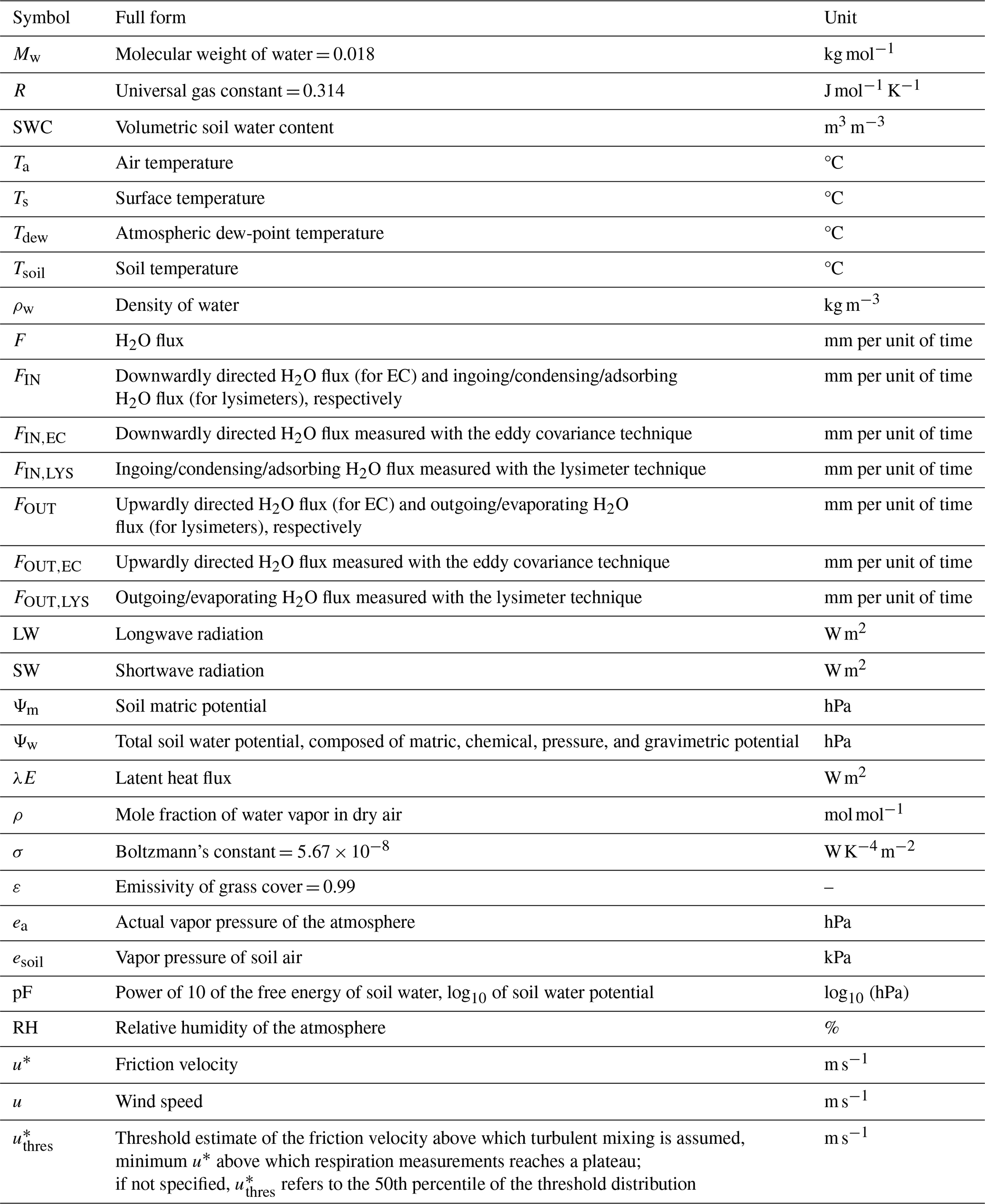
Relative humidity of the air in the soil pore space. Relative humidity (RH, %) was calculated based on Ψm measurements of the heat dissipation sensor and Tsoil at the depth of −0.1 m for each lysimeter column in ES-LMa* based on the Kelvin equation (Edlefsen et al., 1943):
where Ψm, in hPa, is the negative soil water potential; Mw is the molecular weight of water (0.018 kg mol−1); R is the universal gas constant (8.314 ; and ρw is the density of water (1000 kg m−3).
Surface temperature. Surface temperature (Ts, °C) was calculated from measurements of the radiometric tower:
where LW is downwelling (LWIN) and upwelling (LWOUT) longwave radiation (W m−2), σ is Boltzmann's constant (), and ε is emissivity of grass (–) and estimated to be 0.99. Note that this equation is less sensitive to ε compared to the equation form that does not include LWIN (Thakur et al., 2022).
Dew-point temperature. The dew-point temperature (Tdew, °C) was calculated from RH and Ta based on the Magnus equation (λ=17.62, β=243.12) (Sonntag, 1990):
where RH is relative humidity (%) and Ta is air temperature (°C).
Precision and recall. These were calculated to compare the temporal consistency of the flux direction:
where in the case of this study, tp (true positives) denotes the number of observations where the EC method detects a FIN,EC flux simultaneously with (i) at least one and (ii) more than 50 % of the lysimeters detecting FIN,LYS, fp (false positives) denotes observations of FIN,EC where lysimeters detect FOUT,LYS, and fn (false negatives) denotes observations of FOUT,EC while lysimeters detect FIN,LYS.
Table C1List of predictor variables used to model the difference between lysimeter and EC observations of FIN; some variables were given in addition to the half-hourly measurement interval in the form of a rolling average over 24 h (24 h) or normalized by the range of observations of each sensor (norm).
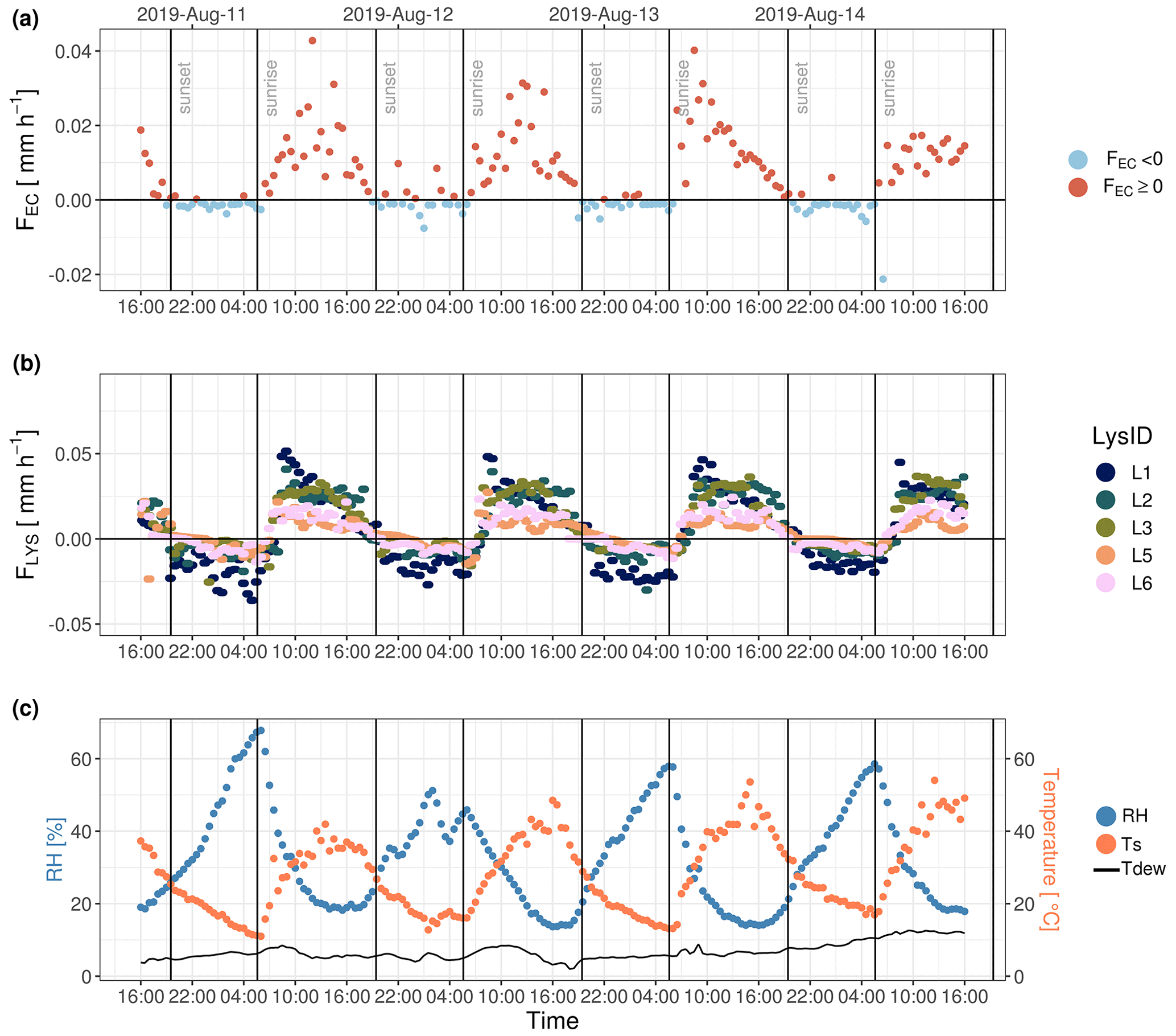
Figure D1Diurnal measurements of water fluxes from (a) eddy covariance (FEC) and (b) the five lysimeters (L1, L2, L3, L5, and L6) from 11 August 2019 at 18:00 CEST until 15 August 2019 at 18:00 CEST at ES-LMa*. Panel (c) illustrates the course of relative humidity (RH) at 2 m height above the soil surface together with surface (Ts) and dew-point temperature (Tdew). Vertical black lines illustrate sunset and sunrise (determined by the geographic coordinates of the field site).
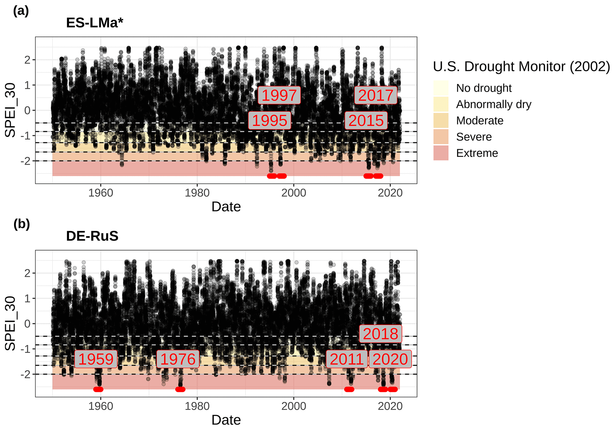
Figure E1Standardized Precipitation Evaporation Index aggregated over 30 d (SPEI_30) from 1950 until 2022 for the (a) Majadas de Tiétar (ES-LMa*) and (b) Selhausen (DE-RuS) field sites. The years with more than 2 weeks of extreme drought, as classified by the US drought monitor (Svoboda et al., 2002), are highlighted by the red points and labels for each site, respectively.
Table F1The u* threshold (m s−1) estimates in ES-LMa* and DE-RuS per year and season. At each site, periods of different surface roughness are considered with a and b representing the dry and wet season in Majadas and unplanted and planted conditions in Selhausen, respectively.
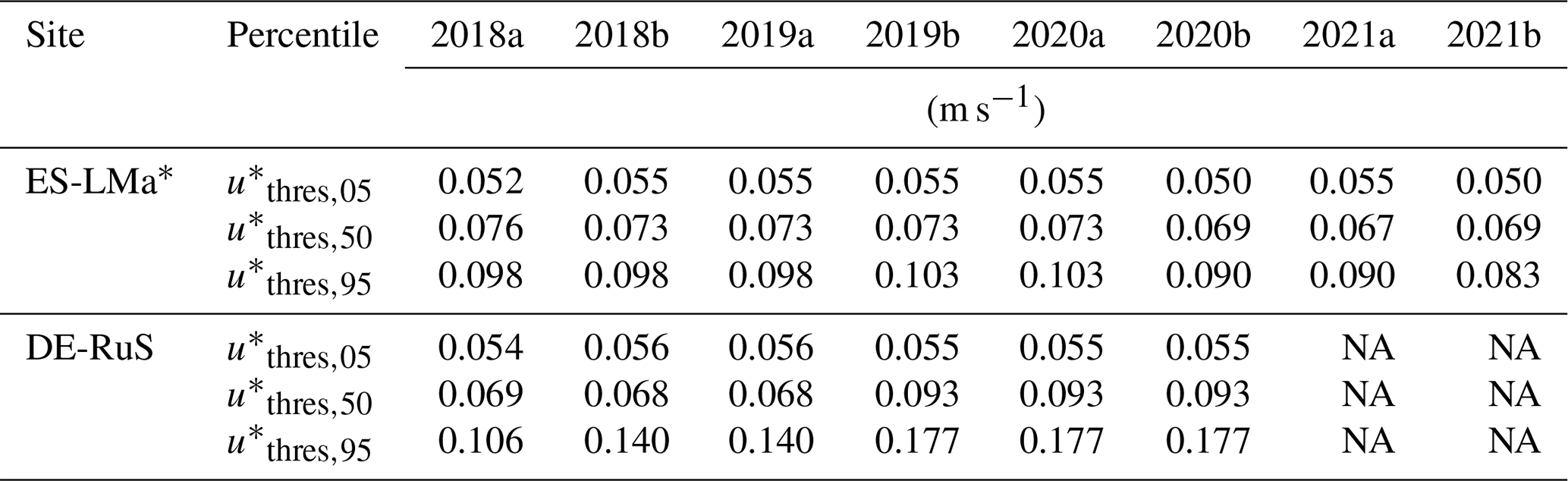
NA: not available.
Table F2Comparison of the number of simultaneous observations of flux direction towards/into the soil between EC and lysimeters for different u* thresholds for ES-LMa* and DE-RuS.
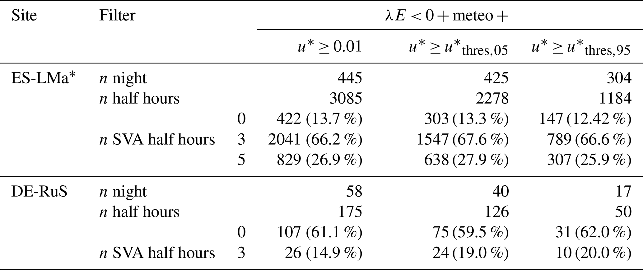
Table F3Statistics for the comparison of FIN,EC and FIN,LYS as nighttime sums in ES-LMa* with different u* filtering thresholds.
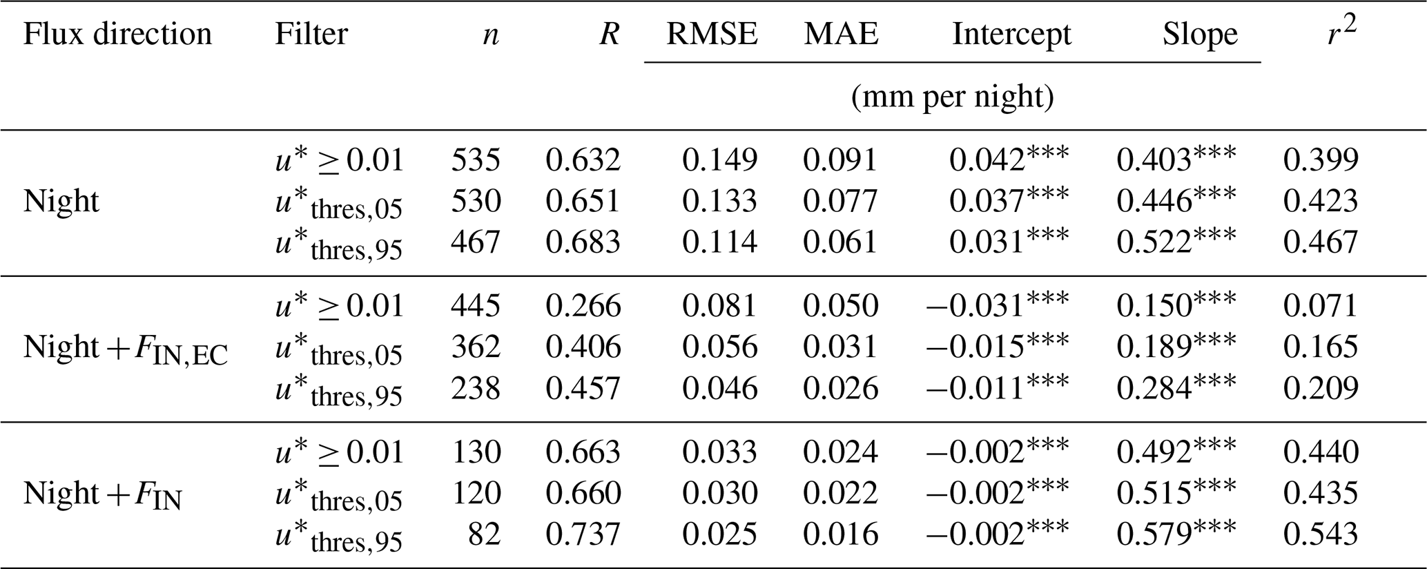
Asterisks represent significance level with * p≤0.05, p≤0.01, p≤0.001.
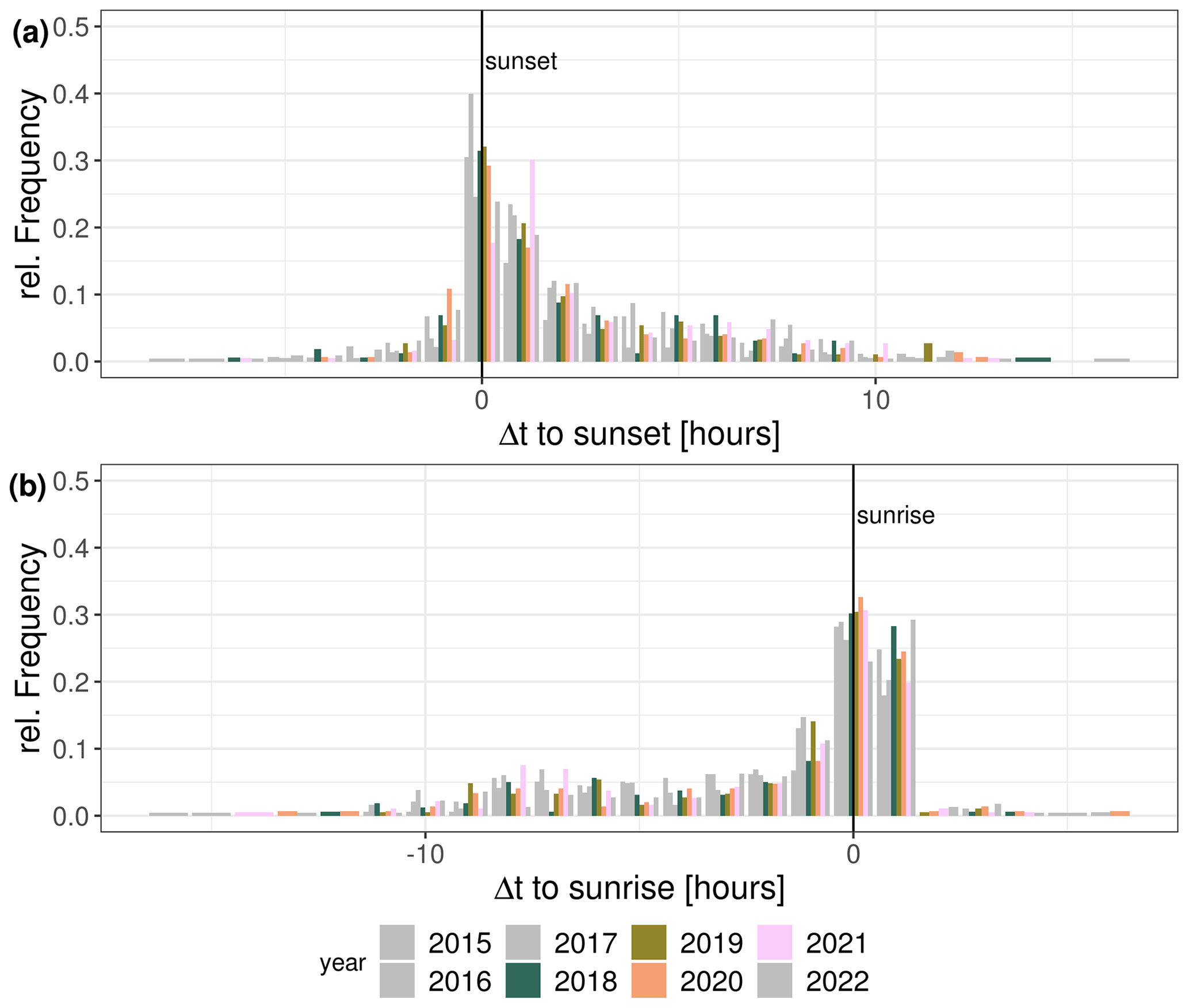
Figure G1Relative frequency of (a) the first and (b) the last negative latent heat flux relative to sunset and sunrise, respectively, for the dry periods within 2015 to 2022 at the Majadas de Tiétar experimental field site. Note that since the dry periods deviate annually, the frequency of the timing is shown relative to the total number of dry days per year.
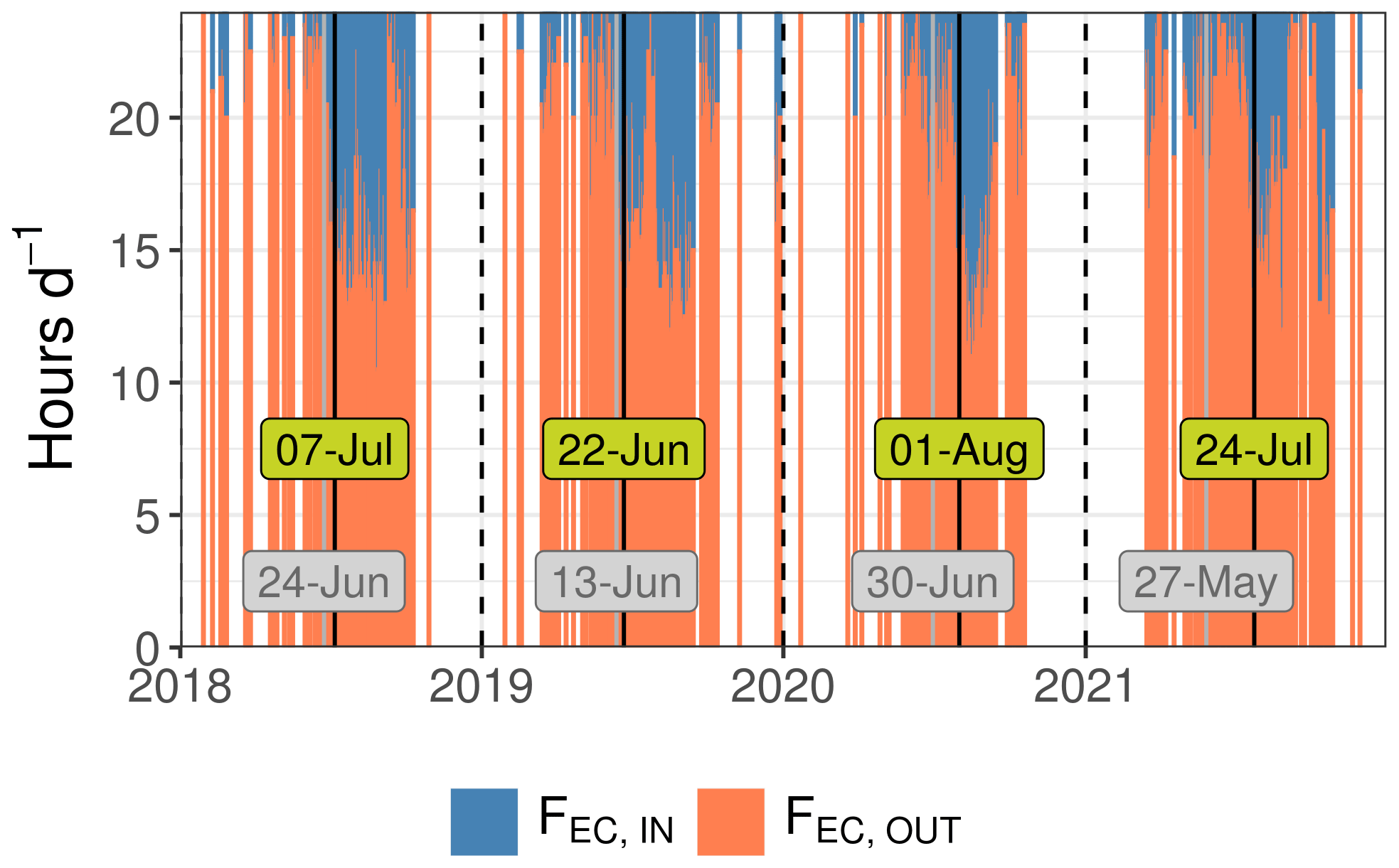
Figure G2Illustration of the diel fraction of positive (red) and negative (blue) λE fluxes measured with the EC method in ES-LMa*. The solid vertical lines mark the onset of adsorption-dominated nights, defined as the first period each year, where 5 consecutive days with more than 4 h of negative latent heat fluxes was observed. Black lines and green labels are based on the EC method, and grey lines with grey labels are based on lysimeter observations.
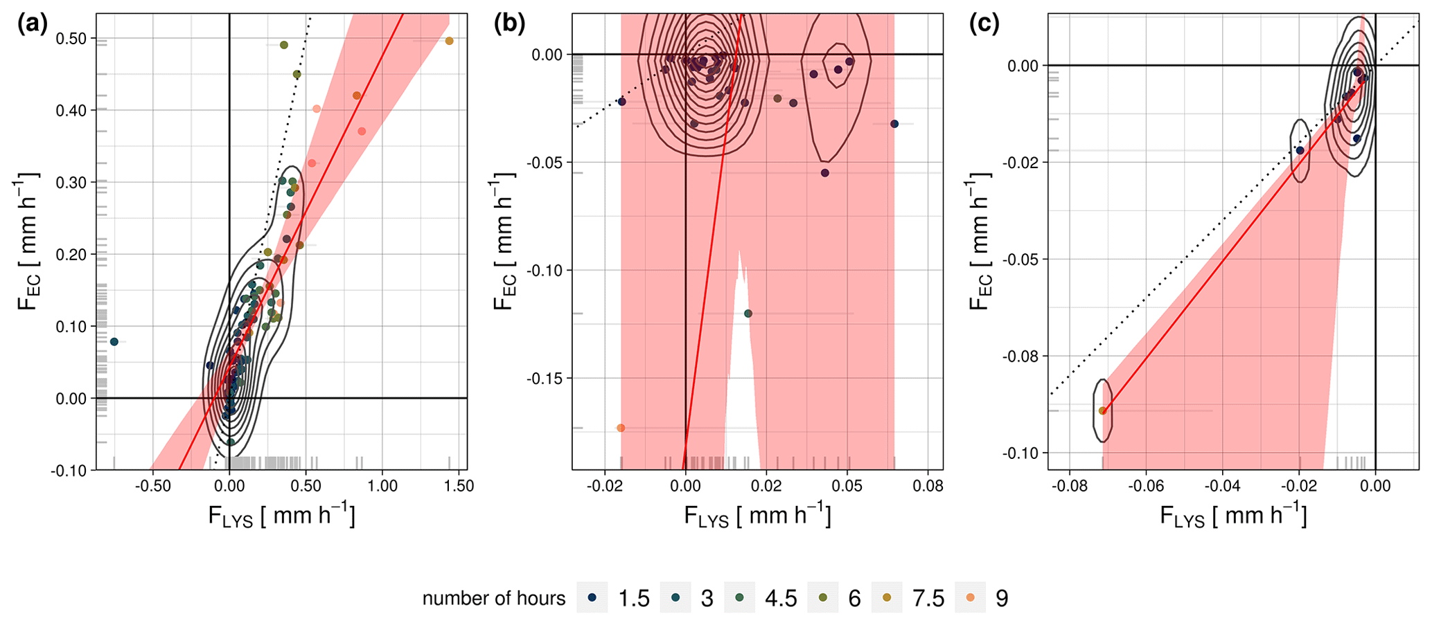
Figure H1Comparison between nighttime sums of lysimeter-measured water fluxes (FLYS) against eddy-covariance-measured fluxes (FEC) in Selhausen (DE-RuS) for different subsets of the data: (a) all good-quality nighttime fluxes, (b) negative EC nighttime fluxes, and (c) negative nighttime fluxes and all lysimeter fluxes classified as soil adsorption of atmospheric vapor. The red line illustrates a major-axis-regression model and the red shading the confidence interval of the model. The dotted black line illustrates identity. Horizontal grey lines illustrate the minimum and maximum sum observed from single lysimeter columns. The color code illustrates the number of hours over which this sum was formed. It depends on how many observations were measured for the respective conditions on each night.
Table H1Statistics for the comparison of FIN,EC and FIN,LYS as nighttime sums in DE-RuS with different filtering periods. See also Fig. H1.
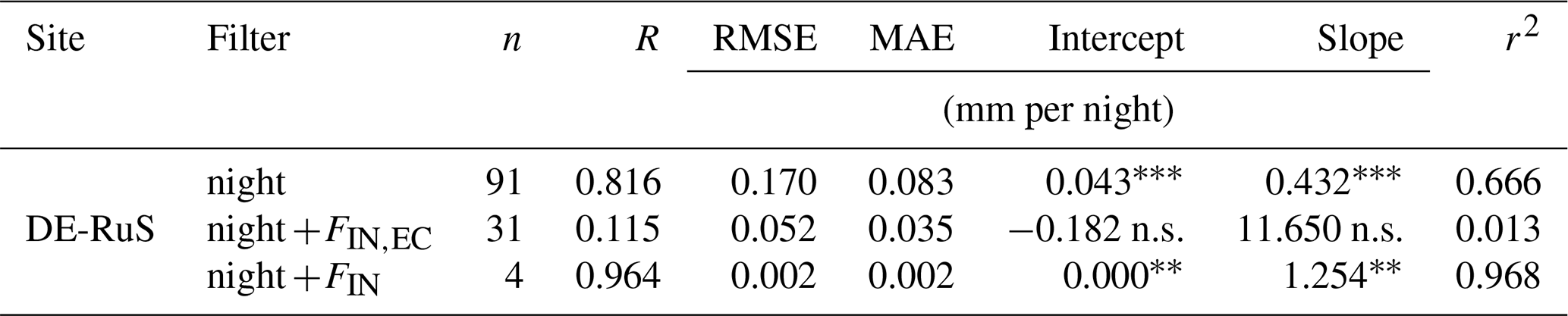
Asterisks represent significance level with * p≤0.05, p≤0.01, p≤0.001. n.s.: not significant.
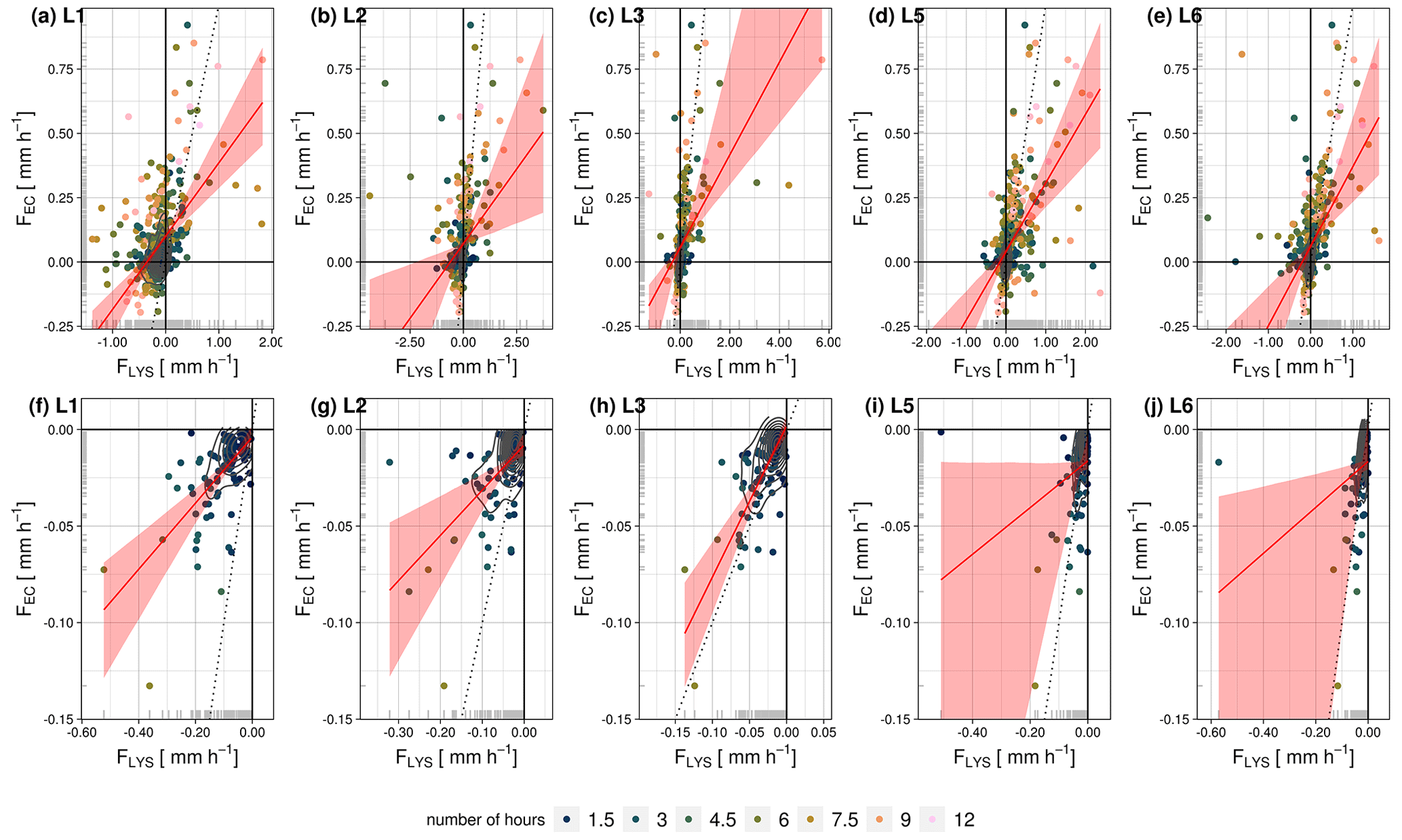
Figure I1Comparison between nighttime sums of lysimeter-measured water fluxes (FLYS) against eddy-covariance-measured fluxes (FEC) in Las Majadas de Tiétar (ES-LMa*) for the individual lysimeters (L1, L2, L3, L5, L6) and for different subsets of the data: (a–e) all good-quality u*-filtered nighttime fluxes; (f–j) good-quality u*-filtered negative nighttime fluxes and all lysimeter fluxes classified as soil adsorption of atmospheric vapor. The red line illustrates a major-axis-regression model and the red shading the confidence interval of the model. The dotted black line illustrates identity. The color code illustrates the number of hours over which this sum was formed. It depends on how many observations were measured for the respective conditions on each night.
Table I1Statistics for the comparison of FIN,EC and FIN,LYS as nighttime sums for each individual lysimeter column in ES-LMa* for different subsets of the data: (1) all good-quality u*-filtered nighttime fluxes and (2) negative nighttime fluxes and all lysimeter fluxes classified as soil adsorption of atmospheric vapor. See also Fig. I1.
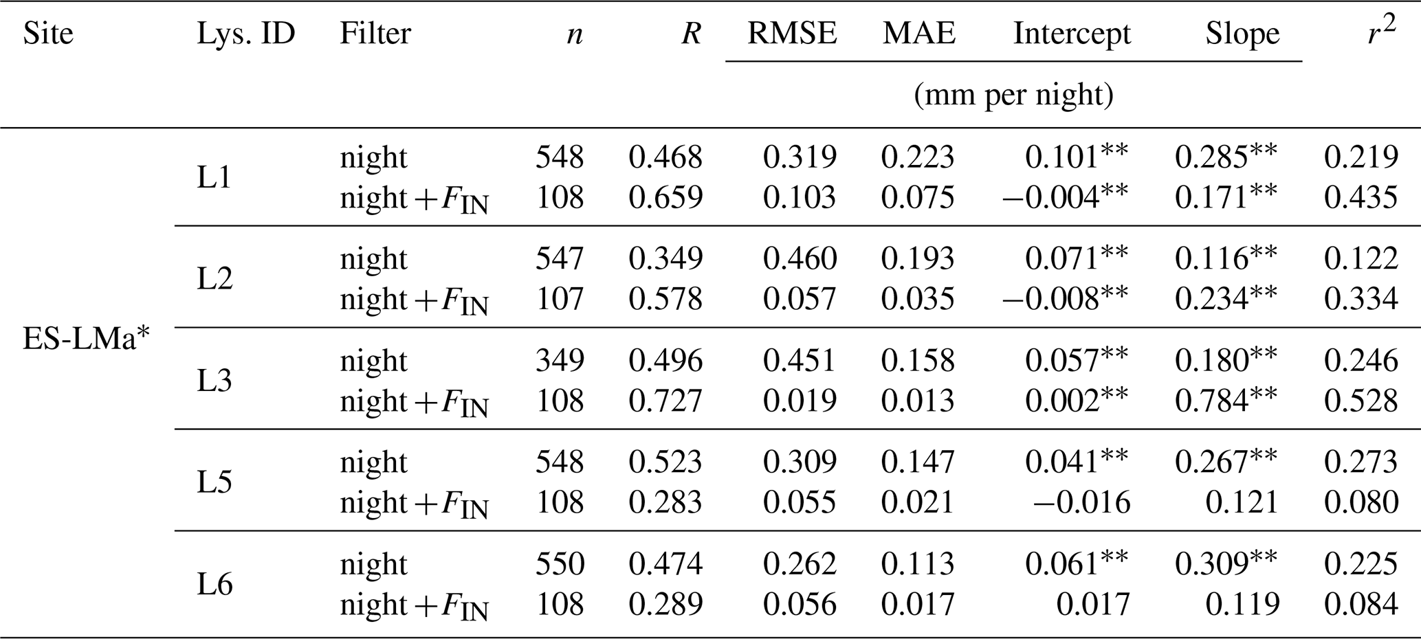
Asterisks represent significance level with * p≤0.05, p≤0.01, p≤0.001.
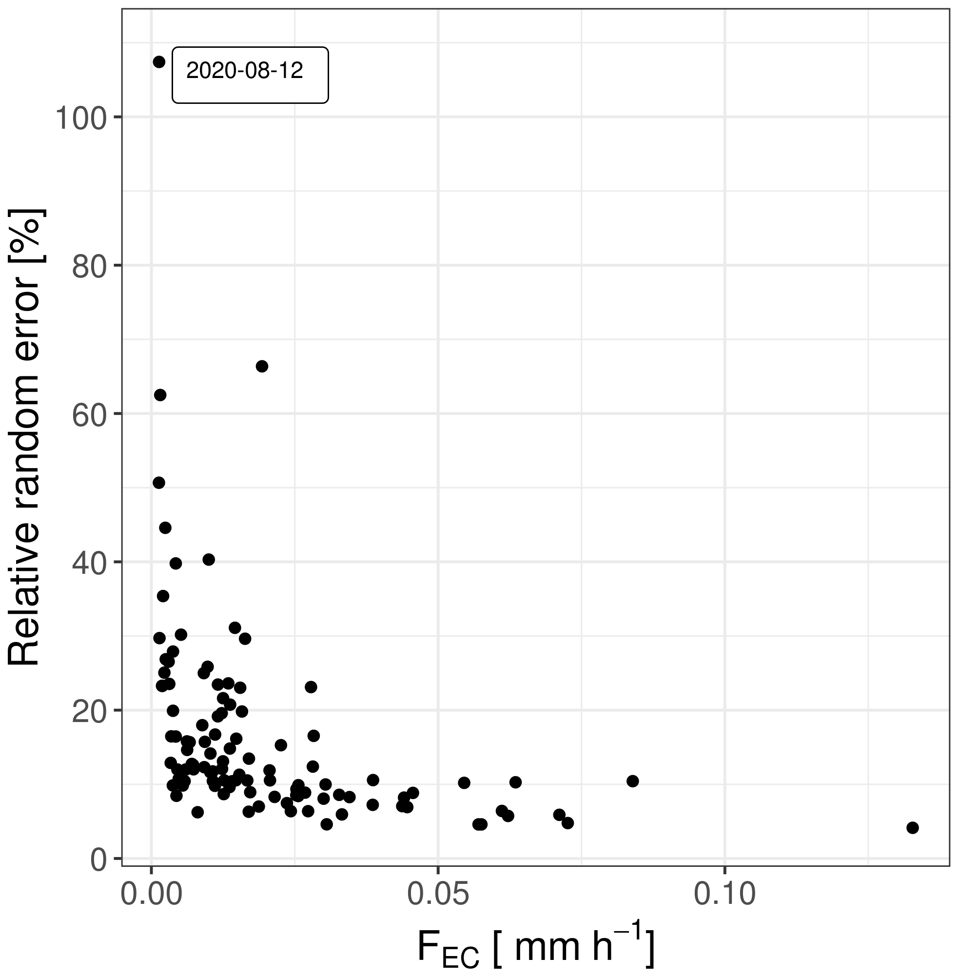
Figure J1The relative random error shown on the y axis is the proportion of the random error from the total inward flux measurements FIN,EC of the EC for each night. The half-hourly FIN,EC measurements per night were summed. The random error per night was determined by propagating the random error in the half-hourly measurements using standard deviations. The date format in the figure is year-month-day.
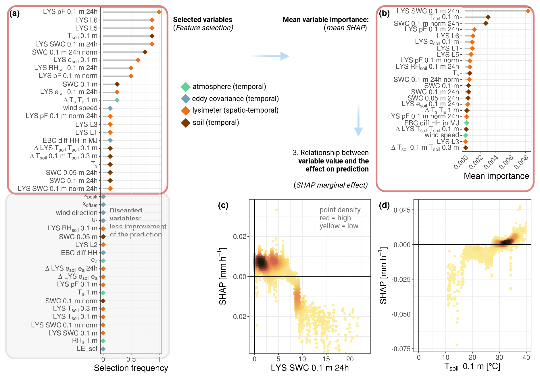
Figure K1Feature selection and variable importance with predictor variable set including lysimeter ID as additional information: (a) selection frequency of predictor variables of the best models; (b) summary graph for variable importance from high to low, based on the ensemble mean SHAP value of each predictor variable; and half-hourly SHAP influence of single observations of the two most important predictor variables – (c) 24 h smoothed SWC within lysimeters at 10 cm depth and (d) soil temperature within lysimeters at 10 cm depth. A description of all predictor variables is given in Appendix C.
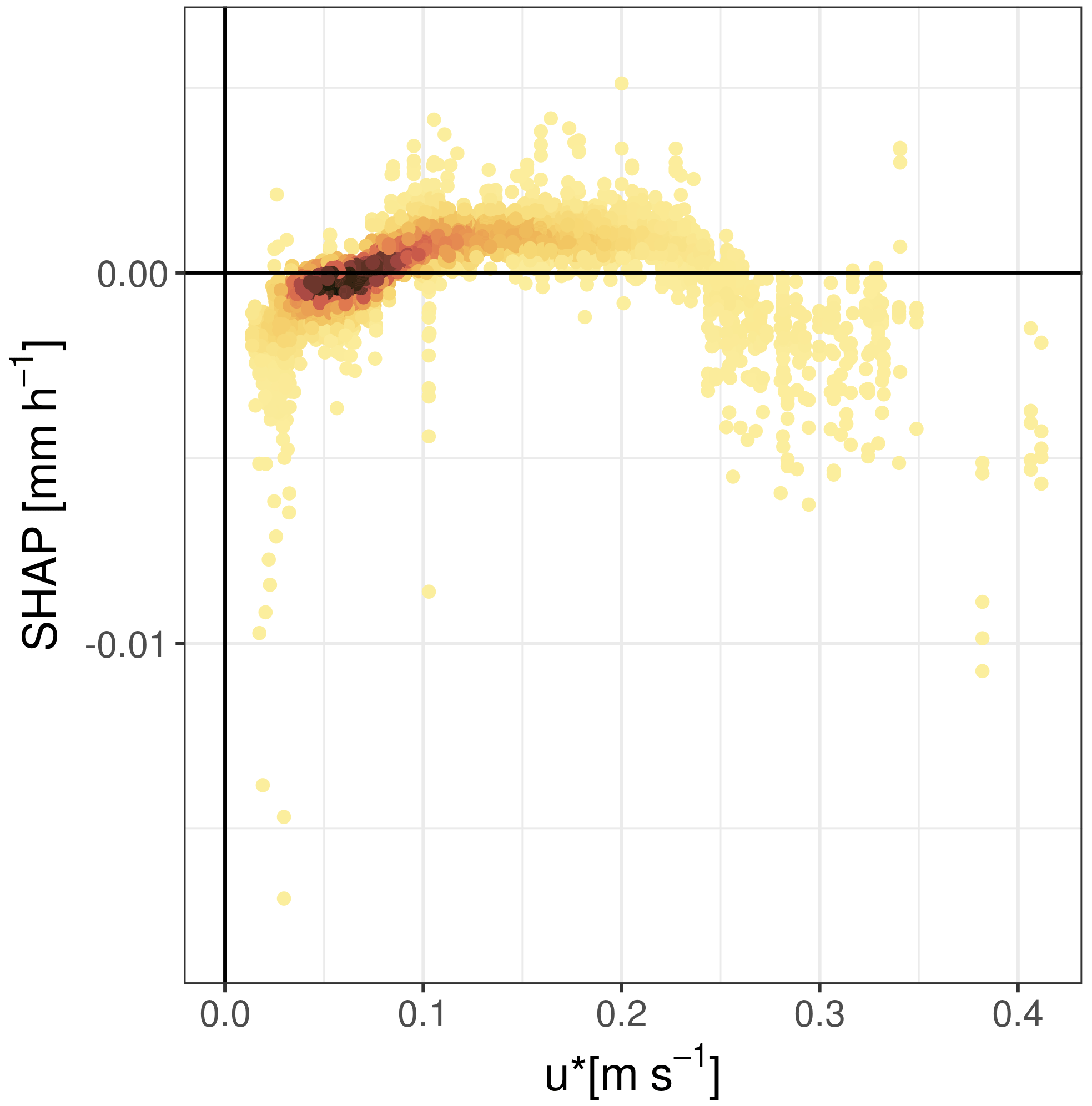
Figure L1Impact of u* on the prediction of the half-hourly differences between lysimeters and EC observations, quantified with SHAP values across the range of observed u* values.
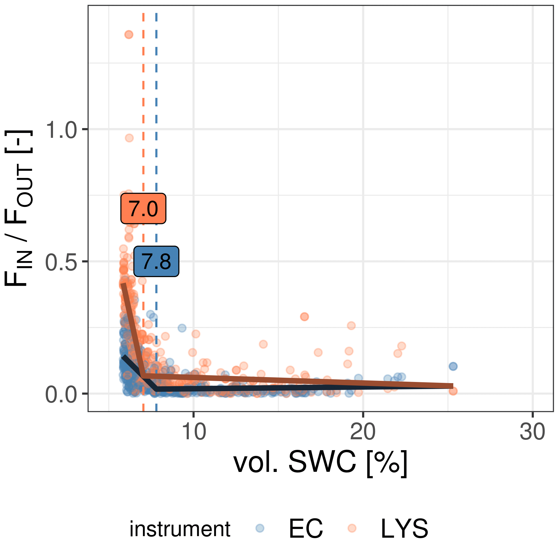
Figure M1Daily ratio of FIN over FOUT across in situ soil water content (SWC) in Majadas de Tiétar measured with lysimeters (red) and the eddy covariance (EC) method (blue). The vertical dashed lines illustrate the breakpoint identified with a segmented linear regression independently for each measurement method.
Data and the R code to reproduce the results of this analysis can be shared on request.
MM, RO, MR, and SJP designed the setup and planned the study. GM, AC, TEM, and MM maintained the ES-LMa* site and the instrumentation and conducted the measurements. SJP and TEM processed the data from ES-LMa*. SJP analyzed the data and prepared the original draft, both under the supervision of MM, RO, AH, and SCL. JG and AG, together with the acknowledged staff, performed the site setup and operation, data processing, and initial quality control for DE-RuS. All authors discussed, reviewed, and edited the paper.
The contact author has declared that none of the authors has any competing interests.
Publisher’s note: Copernicus Publications remains neutral with regard to jurisdictional claims made in the text, published maps, institutional affiliations, or any other geographical representation in this paper. While Copernicus Publications makes every effort to include appropriate place names, the final responsibility lies with the authors.
We thank the city council of Majadas de Tiétar for support. Our thanks go to Martin Strube, Ramón López-Jimenez, Martin Hertel, and the Freiland group at the MPI-BGC for great technical and scientific assistance during fieldwork. Alexander Graf and Jannis Groh thank Marius Schmidt, Daniel Dolfus, Werner Küpper, and Philipp Meulendick for instrument operation and data processing at the DE-RuS site. Sinikka Jasmin Paulus wishes to thank Emmanuel Arthur for sharing his knowledge on estimating soil mineralogy using soil sorption isotherms.
Sinikka Jasmin Paulus has been supported by funding through the International Max Planck Research School for Global Biogeochemical Cycles (IMPRS-gBGC) at the University of Jena. René Orth has been supported by funding from the German Research Foundation (Emmy Noether Grant; grant no. 391059971). The Alexander von Humboldt Foundation has supported this research through the Max Planck Research Prize 2013 to Markus Reichstein. Jannis Groh is funded by the Deutsche Forschungsgemeinschaft (DFG, German Research Foundation) – project no. 460817082. Jannis Groh acknowledges the support of TERENO and SOILCan, which were funded by the Helmholtz Association (HGF) and the Federal Ministry of Education and Research (BMBF).
The article processing charges for this open-access publication were covered by the Max Planck Society.
This paper was edited by Andrew Feldman and reviewed by two anonymous referees.
Amiro, B. D.: Footprint climatologies for evapotranspiration in a boreal catchment, Agr. Forest Meteorol., 90, 195–201, https://doi.org/10.1016/S0168-1923(97)00096-8, 1998. a
Arthur, E., Tuller, M., Moldrup, P., Jensen, D. K., and De Jonge, L. W.: Prediction of clay content from water vapour sorption isotherms considering hysteresis and soil organic matter content, Europ. J. Soil Sci., 66, 206–217, https://doi.org/10.1111/ejss.12191, 2015. a, b
Arthur, E., Tuller, M., Moldrup, P., and de Jonge, L. W.: Evaluation of theoretical and empirical water vapor sorption isotherm models for soils, Water Resour. Res., 52, 190–205, https://doi.org/10.1002/2015WR017681, number: 1, 2016. a, b
Arthur, E., Tuller, M., Norgaard, T., Moldrup, P., and de Jonge, L. W.: Improved estimation of clay content from water content for soils rich in smectite and kaolinite, Geoderma, 350, 40–45, https://doi.org/10.1016/j.geoderma.2019.05.018, 2019. a
Baldocchi, D., Falge, E., Gu, L., Olson, R., Hollinger, D., Running, S., Anthoni, P., Bernhofer, C., Davis, K., Evans, R., Fuentes, J., Goldstein, A., Katul, G., Law, B., Lee, X., Malhi, Y., Meyers, T., Munger, W., Oechel, W., Paw, K. T., Pilegaard, K., Schmid, H. P., Valentini, R., Verma, S., Vesala, T., Wilson, K., and Wofsy, S.: FLUXNET: A New Tool to Study the Temporal and Spatial Variability of Ecosystem–Scale Carbon Dioxide, Water Vapor, and Energy Flux Densities, Bull. Am. Meteorol. Soc., 82, 2415–2434, https://doi.org/10.1175/1520-0477(2001)082<2415:FANTTS>2.3.CO;2, 2001. a
Blume, H.-P., Brümmer, G. W., Fleige, H., Horn, R., Kandeler, E., Kögel-Knabner, I., Kretzschmar, R., Stahr, K., and Wilke, B.-M.: Physical Properties and Processes, 175–283, Springer Berlin Heidelberg, Berlin, Heidelberg, ISBN 978-3-642-30942-7, https://doi.org/10.1007/978-3-642-30942-7_6, 2016a. a
Blume, H.-P., Brümmer, G. W., Fleige, H., Horn, R., Kandeler, E., Kögel-Knabner, I., Kretzschmar, R., Stahr, K., and Wilke, B.-M.: Scheffer/SchachtschabelSoil Science, Springer Berlin Heidelberg, Berlin, Heidelberg, ISBN 978-3-642-30941-0, 978-3-642-30942-7, https://doi.org/10.1007/978-3-642-30942-7, 2016b. a
Bogdanovich, E., Perez-Priego, O., El-Madany, T. S., Guderle, M., Pacheco-Labrador, J., Levick, S. R., Moreno, G., Carrara, A., Pilar Martín, M., and Migliavacca, M.: Using terrestrial laser scanning for characterizing tree structural parameters and their changes under different management in a Mediterranean open woodland, Forest Ecol. Manag., 486, 118945, https://doi.org/10.1016/j.foreco.2021.118945, 2021. a
Bogena, H., Montzka, C., Huisman, J., Graf, A., Schmidt, M., Stockinger, M., von Hebel, C., Hendricks-Franssen, H., van der Kruk, J., Tappe, W., Lücke, A., Baatz, R., Bol, R., Groh, J., Pütz, T., Jakobi, J., Kunkel, R., Sorg, J., and Vereecken, H.: The TERENO-Rur Hydrological Observatory: A Multiscale Multi-Compartment Research Platform for the Advancement of Hydrological Science, Vadose Zone J., 17, 180055, https://doi.org/10.2136/vzj2018.03.0055, 2018. a, b
Breiman, L.: Random forests, Mach. Learn., 45, 5–32, 2001. a
Degré, A., van der Ploeg, M. J., Caldwell, T., and Gooren, H. P.: Comparison of Soil Water Potential Sensors: A Drying Experiment, Vadose Zone J., 16, vzj2016.08.0067, https://doi.org/10.2136/vzj2016.08.0067, 2017. a
de Roode, S. R., Bosveld, F. C., and Kroon, P. S.: Dew Formation, Eddy-Correlation Latent Heat Fluxes, and the Surface Energy Imbalance at Cabauw During Stable Conditions, Bound.-Lay. Meteorol., 135, 369–383, https://doi.org/10.1007/s10546-010-9476-1, 2010. a
Edlefsen, N. and Anderson, A.: Thermodynamics of soil moisture, Hilgardia, 15, 31–298, https://doi.org/10.3733/hilg.v15n02p031, 1943. a, b, c, d
El-Madany, T. S., Griessbaum, F., Fratini, G., Juang, J.-Y., Chang, S.-C., and Klemm, O.: Comparison of sonic anemometer performance under foggy conditions, Agr. Forest Meteorol., 173, 63–73, https://doi.org/10.1016/j.agrformet.2013.01.005, 2013. a
El-Madany, T. S., Reichstein, M., Perez-Priego, O., Carrara, A., Moreno, G., Pilar Martín, M., Pacheco-Labrador, J., Wohlfahrt, G., Nieto, H., Weber, U., Kolle, O., Luo, Y.-P., Carvalhais, N., and Migliavacca, M.: Drivers of spatio-temporal variability of carbon dioxide and energy fluxes in a Mediterranean savanna ecosystem, Agr. Forest Meteorol., 262, 258–278, https://doi.org/10.1016/j.agrformet.2018.07.010, 2018. a, b
El-Madany, T. S., Carrara, A., Martín, M. P., Moreno, G., Kolle, O., Pacheco-Labrador, J., Weber, U., Wutzler, T., Reichstein, M., and Migliavacca, M.: Drought and heatwave impacts on semi-arid ecosystems' carbon fluxes along a precipitation gradient, Philos. T. R. Soc. B, 375, 20190519, https://doi.org/10.1098/rstb.2019.0519, 2020. a
Eugster, W., Burkard, R., Holwerda, F., Scatena, F. N., and Bruijnzeel, L.: Characteristics of fog and fogwater fluxes in a Puerto Rican elfin cloud forest, Agr. Forest Meteorol., 139, 288–306, https://doi.org/10.1016/j.agrformet.2006.07.008, 2006. a
Feigenwinter, C., Franceschi, J., Larsen, J. A., Spirig, R., and Vogt, R.: On the performance of microlysimeters to measure non-rainfall water input in a hyper-arid environment with focus on fog contribution, J. Arid Environ., 182, 104260, https://doi.org/10.1016/j.jaridenv.2020.104260, 2020. a
Florentin, A. and Agam, N.: Estimating non-rainfall-water-inputs-derived latent heat flux with turbulence-based methods, Agr. Forest Meteorol., 247, 533–540, https://doi.org/10.1016/j.agrformet.2017.08.035, 2017. a, b
Foken, T.: The Energy Balance Closure Problem: An Overview, Ecol. Appl., 18, 1351–1367, https://doi.org/10.1890/06-0922.1, 2008. a
Foken, T. and Wichura, B.: Tools for quality assessment of surface-based flux measurements, Agr. Forest Meteorol., 78, 83–105, https://doi.org/10.1016/0168-1923(95)02248-1, 1996. a, b
Fratini, G. and Mauder, M.: Towards a consistent eddy-covariance processing: an intercomparison of EddyPro and TK3, Atmos. Meas. Tech., 7, 2273–2281, https://doi.org/10.5194/amt-7-2273-2014, 2014. a
Fratini, G., Ibrom, A., Arriga, N., Burba, G., and Papale, D.: Relative humidity effects on water vapour fluxes measured with closed-path eddy-covariance systems with short sampling lines, Agr. Forest Meteorol., 165, 53–63, https://doi.org/10.1016/j.agrformet.2012.05.018, 2012. a, b
Garcia Gonzalez, R., Verhoef, A., Luigi Vidale, P., and Braud, I.: Incorporation of water vapor transfer in the JULES land surface model: Implications for key soil variables and land surface fluxes, Water Resour. Res., 48, https://doi.org/10.1029/2011WR011811, 2012. a
Gebler, S., Hendricks Franssen, H.-J., Pütz, T., Post, H., Schmidt, M., and Vereecken, H.: Actual evapotranspiration and precipitation measured by lysimeters: a comparison with eddy covariance and tipping bucket, Hydrol. Earth Syst. Sci., 19, 2145–2161, https://doi.org/10.5194/hess-19-2145-2015, 2015. a
Groh, J., Vanderborght, J., Pütz, T., and Vereecken, H.: How to Control the Lysimeter Bottom Boundary to Investigate the Effect of Climate Change on Soil Processes?, Vadose Zone J., 15, vzj2015.08.0113, https://doi.org/10.2136/vzj2015.08.0113, 2016. a
Groh, J., Vanderborght, J., Pütz, T., Vogel, H.-J., Gründling, R., Rupp, H., Rahmati, M., Sommer, M., Vereecken, H., and Gerke, H. H.: Responses of soil water storage and crop water use efficiency to changing climatic conditions: a lysimeter-based space-for-time approach, Hydrol. Earth Syst. Sci., 24, 1211–1225, https://doi.org/10.5194/hess-24-1211-2020, 2020. a
Groh, J., Diamantopoulos, E., Duan, X., Ewert, F., Heinlein, F., Herbst, M., Holbak, M., Kamali, B., Kersebaum, K.-C., Kuhnert, M., Nendel, C., Priesack, E., Steidl, J., Sommer, M., Pütz, T., Vanderborght, J., Vereecken, H., Wallor, E., Weber, T. K. D., Wegehenkel, M., Weihermüller, L., and Gerke, H. H.: Same soil, different climate: Crop model intercomparison on translocated lysimeters, Vadose Zone J., 21, e20202, https://doi.org/10.1002/vzj2.20202, 2022. a
Han, Q., Wang, T., Wang, L., Smettem, K., Mai, M., and Chen, X.: Comparison of Nighttime With Daytime Evapotranspiration Responses to Environmental Controls Across Temporal Scales Along a Climate Gradient, Water Resour. Res., 57, e2021WR029638, https://doi.org/10.1029/2021WR029638, 2021. a
Hansen, H. C.: The Water-Retaining Power of the Soil, J. Ecol., 14, 111, https://doi.org/10.2307/2255784, 1926. a
Heiskanen, J., Brümmer, C., Buchmann, N., Calfapietra, C., Chen, H., Gielen, B., Gkritzalis, T., Hammer, S., Hartman, S., Herbst, M., Janssens, I. A., Jordan, A., Juurola, E., Karstens, U., Kasurinen, V., Kruijt, B., Lankreijer, H., Levin, I., Linderson, M.-L., Loustau, D., Merbold, L., Myhre, C. L., Papale, D., Pavelka, M., Pilegaard, K., Ramonet, M., Rebmann, C., Rinne, J., Rivier, L., Saltikoff, E., Sanders, R., Steinbacher, M., Steinhoff, T., Watson, A., Vermeulen, A. T., Vesala, T., Vítková, G., and Kutsch, W.: The Integrated Carbon Observation System in Europe, Bull. Am. Meteorol. Soc., 103, E855–E872, https://doi.org/10.1175/BAMS-D-19-0364.1, 2022. a
Hirschi, M., Michel, D., Lehner, I., and Seneviratne, S. I.: A site-level comparison of lysimeter and eddy covariance flux measurements of evapotranspiration, Hydrol. Earth Syst. Sci., 21, 1809–1825, https://doi.org/10.5194/hess-21-1809-2017, 2017. a
Hollinger, D. Y. and Richardson, A. D.: Uncertainty in eddy covariance measurements and its application to physiological models, Tree Physiol., 25, 873–885, https://doi.org/10.1093/treephys/25.7.873, 2005. a
ICOS: DE-RuS ICOS Ecosystem Station Labelling Report, https://hdl.handle.net/11676/HE7Nj8_yV0xTr1zYLvOchSR1 (last access: 14 April 2024), 2021. a
Jackisch, C., Germer, K., Graeff, T., Andrä, I., Schulz, K., Schiedung, M., Haller-Jans, J., Schneider, J., Jaquemotte, J., Helmer, P., Lotz, L., Bauer, A., Hahn, I., Šanda, M., Kumpan, M., Dorner, J., de Rooij, G., Wessel-Bothe, S., Kottmann, L., Schittenhelm, S., and Durner, W.: Soil moisture and matric potential – an open field comparison of sensor systems, Earth Syst. Sci. Data, 12, 683–697, https://doi.org/10.5194/essd-12-683-2020, 2020. a
Jiang, C., Séquaris, J.-M., Wacha, A., Bóta, A., Vereecken, H., and Klumpp, E.: Effect of metal oxide on surface area and pore size of water-dispersible colloids from three German silt loam topsoils, Geoderma, 235/236, 260–270, https://doi.org/10.1016/j.geoderma.2014.07.017, 2014. a
Jung, M. and Zscheischler, J.: A Guided Hybrid Genetic Algorithm for Feature Selection with Expensive Cost Functions, Procedia Comput. Sci., 18, 2337–2346, https://doi.org/10.1016/j.procs.2013.05.405, 2013. a, b
Kidron, G. J.: A simple weighing method for dew and fog measurements, Weather, 53, 428–433, https://doi.org/10.1002/j.1477-8696.1998.tb06362.x, 1998. a
Kidron, G. J. and Kronenfeld, R.: Assessing the effect of micro-lysimeters on NRWI: Do micro-lysimeters adequately represent the water input of natural soil?, J. Hydrol., 548, 382–390, https://doi.org/10.1016/j.jhydrol.2017.03.005, 2017. a
Kidron, G. J. and Kronenfeld, R.: Microlysimeters overestimate the amount of non-rainfall water – an experimental approach, CATENA, 194, 104691, https://doi.org/10.1016/j.catena.2020.104691, 2020. a
Kidron, G. J. and Starinsky, A.: Measurements and ecological implications of non‐rainfall water in desert ecosystems – A review, Ecohydrology, 12, e2121, https://doi.org/10.1002/eco.2121, 2019. a, b
Kljun, N., Calanca, P., Rotach, M. W., and Schmid, H. P.: A simple two-dimensional parameterisation for Flux Footprint Prediction (FFP), Geosci. Model Dev., 8, 3695–3713, https://doi.org/10.5194/gmd-8-3695-2015, 2015. a
Kool, D., Agra, E., Drabkin, A., Duncan, A., Fendinat, P., Leduc, S., Lupovitch, G., Nambwandja, A., Ndilenga, N., Nguyẽn Thị, T., Poodiack, B., Sagi, L., Shmuel, Y., Maggs-Kölling, G., Marais, E., Pinshow, B., Turner, J., and Agam, N.: The overlooked non-rainfall water input sibling of fog and dew: Daily water vapor adsorption on a Nara hummock in the Namib Sand Sea, J. Hydrol., 598, 126420, https://doi.org/10.1016/j.jhydrol.2021.126420, 2021. a
Kosmas, C., Marathianou, M., Gerontidis, S., Detsis, V., Tsara, M., and Poesen, J.: Parameters affecting water vapor adsorption by the soil under semi-arid climatic conditions, Agr. Water Manag., 48, 61–78, https://doi.org/10.1016/S0378-3774(00)00113-X, 2001. a
Lasslop, G., Reichstein, M., Kattge, J., and Papale, D.: Influences of observation errors in eddy flux data on inverse model parameter estimation, Biogeosciences, 5, 1311–1324, https://doi.org/10.5194/bg-5-1311-2008, 2008. a
Legendre, P.: lmodel2: Model II Regression, R package version 1.7-3 [code], https://CRAN.R-project.org/package=lmodel2 (last access: 14 April 2024), 2018. a
Lopez-Canfin, C., Lázaro, R., and Sánchez-Cañete, E. P.: Water vapor adsorption by dry soils: A potential link between the water and carbon cycles, Sci. Total Environ., 824, 153746, https://doi.org/10.1016/j.scitotenv.2022.153746, 2022. a
Lundberg, S. M. and Lee, S.-I.: A unified approach to interpreting model predictions, in: Advances in neural information processing systems 30: annual conference on neural information processing systems 2017, December 4–9, 2017, Long Beach, CA, USA, 4765–4774, 2017. a
Luo, Y., El-Madany, T. S., Filippa, G., Ma, X., Ahrens, B., Carrara, A., Gonzalez-Cascon, R., Cremonese, E., Galvagno, M., Hammer, T. W., Pacheco-Labrador, J., Martín, M. P., Moreno, G., Perez-Priego, O., Reichstein, M., Richardson, A. D., Römermann, C., and Migliavacca, M.: Using Near-Infrared-Enabled Digital Repeat Photography to Track Structural and Physiological Phenology in Mediterranean Tree – Grass Ecosystems, Remote Sens., 10, 1293, https://doi.org/10.3390/rs10081293, 2018. a
Massman, W. and Lee, X.: Eddy covariance flux corrections and uncertainties in long-term studies of carbon and energy exchanges, Agr. Forest Meteorol., 113, 121–144, https://doi.org/10.1016/S0168-1923(02)00105-3, 2002. a
Mauder, M. and Foken, T.: Documentation and instruction manual of the eddy-covariance software package TK3, https://epub.uni-bayreuth.de/id/eprint/342/1/ARBERG046.pdf (last access: 14 April 2024), 2011. a
Mauder, M., Cuntz, M., Drüe, C., Graf, A., Rebmann, C., Schmid, H. P., Schmidt, M., and Steinbrecher, R.: A strategy for quality and uncertainty assessment of long-term eddy-covariance measurements, Agr. Forest Meteorol., 169, 122–135, https://doi.org/10.1016/j.agrformet.2012.09.006, 2013. a, b
Mauder, M., Genzel, S., Fu, J., Kiese, R., Soltani, M., Steinbrecher, R., Zeeman, M., Banerjee, T., De Roo, F., and Kunstmann, H.: Evaluation of energy balance closure adjustment methods by independent evapotranspiration estimates from lysimeters and hydrological simulations, Hydrol. Process., 32, 39–50, https://doi.org/10.1002/hyp.11397, 2018. a, b
Mauder, M., Foken, T., and Cuxart, J.: Surface-Energy-Balance Closure over Land: A Review, Bound.-Lay. Meteorol., 177, 395–426, https://doi.org/10.1007/s10546-020-00529-6, 2020. a
McHugh, T. A., Morrissey, E. M., Reed, S. C., Hungate, B. A., and Schwartz, E.: Water from air: an overlooked source of moisture in arid and semiarid regions, Sci. Rep., 5, 13767, https://doi.org/10.1038/srep13767, 2015. a
Migliavacca, M., Perez-Priego, O., Rossini, M., El-Madany, T. S., Moreno, G., van der Tol, C., Rascher, U., Berninger, A., Bessenbacher, V., Burkart, A., Carrara, A., Fava, F., Guan, J.-H., Hammer, T. W., Henkel, K., Juarez-Alcalde, E., Julitta, T., Kolle, O., Martín, M. P., Musavi, T., Pacheco-Labrador, J., Pérez-Burgueño, A., Wutzler, T., Zaehle, S., and Reichstein, M.: Plant functional traits and canopy structure control the relationship between photosynthetic CO 2 uptake and far-red sun-induced fluorescence in a Mediterranean grassland under different nutrient availability, New Phytol., 214, 1078–1091, https://doi.org/10.1111/nph.14437, 2017. a
Miralles, D. G., Brutsaert, W., Dolman, A. J., and Gash, J. H.: On the Use of the Term “Evapotranspiration”, Water Resour. Res., 56, e2020WR028055, https://doi.org/10.1029/2020WR028055, 2020. a
Moncrieff, J. B., Massheder, J. M., de Bruin, H., Elbers, J., Friborg, T., Heusinkveld, B., Kabat, P., Scott, S., Soegaard, H., and Verhoef, A.: A system to measure surface fluxes of momentum, sensible heat, water vapour and carbon dioxide, J. Hydrol., 188/189, 589–611, https://doi.org/10.1016/S0022-1694(96)03194-0, 1997. a
Moro, M. J., Were, A., Villagarcıa, L., Canton, Y., and Domingo, F.: Dew measurement by Eddy covariance and wetness sensor in a semiarid ecosystem of SE Spain, J. Hydrol., 335, 295–302, https://doi.org/10.1016/j.jhydrol.2006.11.019, 2007. a
Nair, R. K. F., Morris, K. A., Hertel, M., Luo, Y., Moreno, G., Reichstein, M., Schrumpf, M., and Migliavacca, M.: N : P stoichiometry and habitat effects on Mediterranean savanna seasonal root dynamics, Biogeosciences, 16, 1883–1901, https://doi.org/10.5194/bg-16-1883-2019, 2019. a
NC Geological Survey of Spain (IGME): MAPA GEOLÓGICO DE ESPAÑA Escala 1:50 000 – NAVALMORAL DE LA MATA., https://info.igme.es/cartografiadigital/datos/magna50/memorias/MMagna0624.pdf (last access: 14 April 2024), 1992. a
Ney, P. and Graf, A.: High-Resolution Vertical Profile Measurements for Carbon Dioxide and Water Vapour Concentrations Within and Above Crop Canopies, Bound.-Lay. Meteorol., 166, 449–473, https://doi.org/10.1007/s10546-017-0316-4, 2018. a
Or, D., Smets, B. F., Wraith, J. M., Dechesne, A., and Friedman, S. P.: Physical constraints affecting bacterial habitats and activity in unsaturated porous media – a review, Adv. Water Resour., 30, 1505–1527, https://doi.org/10.1016/j.advwatres.2006.05.025, 2007. a
Or, D., Lehmann, P., Shahraeeni, E., and Shokri, N.: Advances in Soil Evaporation Physics-A Review, Vadose Zone J., 12, vzj2012.0163, https://doi.org/10.2136/vzj2012.0163, 2013. a, b
Or, D., Tuller, M., and Wraith, J. M.: Water potential, in: Reference Module in Earth Systems and Environmental Sciences, Elsevier, ISBN 978-0-12-409548-9, https://doi.org/10.1016/B978-0-12-822974-3.00114-2, 2022. a
Orchiston, H. D.: Adsorption of water vapor: I. Soils at 25 °C, Soil Sci., 76, 453–466, https://doi.org/10.1097/00010694-195312000-00005, 1953. a
Orchiston, H. D.: Adsorption of water vapor: II Clays at 25 °C, Soil Sci., 78, 463–480, 1954. a
Padrón, R. S., Gudmundsson, L., Michel, D., and Seneviratne, S. I.: Terrestrial water loss at night: global relevance from observations and climate models, Hydrol. Earth Syst. Sci., 24, 793–807, https://doi.org/10.5194/hess-24-793-2020, 2020. a
Papale, D., Reichstein, M., Aubinet, M., Canfora, E., Bernhofer, C., Kutsch, W., Longdoz, B., Rambal, S., Valentini, R., Vesala, T., and Yakir, D.: Towards a standardized processing of Net Ecosystem Exchange measured with eddy covariance technique: algorithms and uncertainty estimation, Biogeosciences, 3, 571–583, https://doi.org/10.5194/bg-3-571-2006, 2006. a
Passioura, J.: Water transport in and to roots, Ann. Rev. Plant Phys., 39, 245–265, 1988. a
Paulus, S. J., El-Madany, T. S., Orth, R., Hildebrandt, A., Wutzler, T., Carrara, A., Moreno, G., Perez-Priego, O., Kolle, O., Reichstein, M., and Migliavacca, M.: Resolving seasonal and diel dynamics of non-rainfall water inputs in a Mediterranean ecosystem using lysimeters, Hydrol. Earth Syst. Sci., 26, 6263–6287, https://doi.org/10.5194/hess-26-6263-2022, 2022. a, b, c, d, e, f, g, h
Perez-Priego, O., El-Madany, T. S., Migliavacca, M., Kowalski, A. S., Jung, M., Carrara, A., Kolle, O., Martín, M. P., Pacheco-Labrador, J., Moreno, G., and Reichstein, M.: Evaluation of eddy covariance latent heat fluxes with independent lysimeter and sapflow estimates in a Mediterranean savannah ecosystem, Agr. Forest Meteorol., 236, 87–99, https://doi.org/10.1016/j.agrformet.2017.01.009, 2017. a, b, c
Peters, A., Nehls, T., Schonsky, H., and Wessolek, G.: Separating precipitation and evapotranspiration from noise – a new filter routine for high-resolution lysimeter data, Hydrol. Earth Syst. Sci., 18, 1189–1198, https://doi.org/10.5194/hess-18-1189-2014, 2014. a, b
Peters, A., Nehls, T., and Wessolek, G.: Technical note: Improving the AWAT filter with interpolation schemes for advanced processing of high resolution data, Hydrol. Earth Syst. Sci., 20, 2309–2315, https://doi.org/10.5194/hess-20-2309-2016, 2016. a, b
Peters, A., Groh, J., Schrader, F., Durner, W., Vereecken, H., and Pütz, T.: Towards an unbiased filter routine to determine precipitation and evapotranspiration from high precision lysimeter measurements, J. Hydrol., 549, 731–740, https://doi.org/10.1016/j.jhydrol.2017.04.015, 2017. a, b
Philip, J. and De Vries, D.: Moisture movement in porous materials under temperature gradients, Eos, Transactions American Geophysical Union, 38, 222–232, 1957. a
Podlasly, C. and Schwärzel, K.: Development of a Continuous Closed Pipe System for Controlling Soil Temperature at the Lower Boundary of Weighing Field Lysimeters, Soil Sci. Soc. Am. J., 77, 2157–2163, https://doi.org/10.2136/sssaj2013.03.0113n, 2013. a
Pohl, F., Rakovec, O., Rebmann, C., Hildebrandt, A., Boeing, F., Hermanns, F., Samaniego, L., Attinger, S., and Kumar, R.: Long-term daily hydrometeorological drought indices, soil moisture, and evapotranspiration for ICOS ecosystem sites, Zenodo [data set], https://doi.org/10.5281/zenodo.7561854, 2022. a, b
Pohl, F., Rakovec, O., Rebmann, C., Hildebrandt, A., Boeing, F., Hermanns, F., Attinger, S., Samaniego, L., and Kumar, R.: Long-term daily hydrometeorological drought indices, soil moisture, and evapotranspiration for ICOS sites, Sci. Data, 10, 281, https://doi.org/10.1038/s41597-023-02192-1, 2023. a
Pütz, T. and Groh, J.: Lysimetry, in: Encyclopedia of Soils in the Environment (Second Edition), edited by: Goss, M. J. and Oliver, M., 667–679, Academic Press, Oxford, ISBN 978-0-323-95133-3, https://doi.org/10.1016/B978-0-12-822974-3.00272-X, 2023. a, b
Pütz, T., Kiese, R., Wollschläger, U., Groh, J., Rupp, H., Zacharias, S., Priesack, E., Gerke, H. H., Gasche, R., Bens, O., Borg, E., Baessler, C., Kaiser, K., Herbrich, M., Munch, J.-C., Sommer, M., Vogel, H.-J., Vanderborght, J., and Vereecken, H.: TERENO-SOILCan: a lysimeter-network in Germany observing soil processes and plant diversity influenced by climate change, Environ. Earth Sci., 75, 1242, https://doi.org/10.1007/s12665-016-6031-5, 2016. a, b, c, d
Pütz, T., Fank, J., and Flury, M.: Lysimeters in Vadose Zone Research, Vadose Zone J., 17, 180035, https://doi.org/10.2136/vzj2018.02.0035, 2018. a
Qubaja, R., Amer, M., Tatarinov, F., Rotenberg, E., Preisler, Y., Sprintsin, M., and Yakir, D.: Partitioning evapotranspiration and its long-term evolution in a dry pine forest using measurement-based estimates of soil evaporation, Agr. Forest Meteorol., 281, 107831, https://doi.org/10.1016/j.agrformet.2019.107831, 2020. a, b
Rebmann, C., Göckede, M., Foken, T., et al.: Quality analysis applied on eddy covariance measurements at complex forest sites using footprint modelling, Theor. Appl. Climatol. 80, 121–141, https://doi.org/10.1007/s00704-004-0095-y, 2005. a
Reth, S., Perez-Priego, O., Coners, H., and Nolz, R.: Lysimeter, Springer International Publishing, Cham, 1583–1593, ISBN 978-3-030-52171-4, https://doi.org/10.1007/978-3-030-52171-4_58, 2021. a
Saaltink, M. W., Kohfahl, C., and Molano‐Leno, L.: Analysis of water vapor adsorption in soils by means of a lysimeter and numerical modeling, Vadose Zone J., 19, e20012, https://doi.org/10.1002/vzj2.20012, 2020. a, b, c, d, e, f, g
Sakai, M., Toride, N., and Šimůnek, J.: Water and Vapor Movement with Condensation and Evaporation in a Sandy Column, Soil Sci. Soc. Am. J., 73, 707–717, https://doi.org/10.2136/sssaj2008.0094, 2009. a
Schmid, H. P.: Source areas for scalars and scalar fluxes, Bound.-Lay. Meteorol., 67, 293–318, https://doi.org/10.1007/BF00713146, 1994. a
Schmid, H. P.: Footprint modeling for vegetation atmosphere exchange studies: a review and perspective, Agr. Forest Meteorol., 113, 159–183, https://doi.org/10.1016/S0168-1923(02)00107-7, 2002. a
Schneider, J., Rothfuss, Y., Groh, J., Vereecken, H., Pütz, T., Helmig, R., and Vanderborght, J.: Prediction of soil evaporation measured with weighable lysimeters using the FAO Penman – Monteith method in combination with Richards' equation, Vadose Zone J., 20, e20102, https://doi.org/10.1002/vzj2.20102, 2021. a
Sonntag, D.: Important new values of the physical constants of 1986, vapour pressure formulations based on the ITS-90, and psychrometer formulae, Z. Meteorol., 40, 340–344, 1990. a, b, c
Svoboda, M., LeComte, D., Hayes, M., Heim, R., Gleason, K., Angel, J., Rippey, B., Tinker, R., Palecki, M., Stooksbury, D., Miskus, D., and Stephens, S.: The drought monitor, Bull. Am. Meteorol. Soc., 83, 1181–1190, https://doi.org/10.1175/1520-0477-83.8.1181, 2002. a, b
Thakur, G., Schymanski, S. J., Mallick, K., Trebs, I., and Sulis, M.: Downwelling longwave radiation and sensible heat flux observations are critical for surface temperature and emissivity estimation from flux tower data, Sci. Rep., 12, 8592, https://doi.org/10.1038/s41598-022-12304-3, 2022. a
Thieurmel, B. and Elmarhraoui, A.: suncalc: Compute Sun Position, Sunlight Phases, Moon Position and Lunar Phase, R package version 0.5.1 [code], https://CRAN.R-project.org/package=suncalc (last access: 14 April 2024), 2022. a
Tuller, M., Or, D., and Dudley, L. M.: Adsorption and capillary condensation in porous media: Liquid retention and interfacial configurations in angular pores, Water Resour. Res., 35, 1949–1964, https://doi.org/10.1029/1999WR900098, 1999. a, b
Uclés, O., Villagarcía, L., Cantón, Y., and Domingo, F.: Microlysimeter station for long term non-rainfall water input and evaporation studies, Agr. Forest Meteorol., 182/183, 13–20, https://doi.org/10.1016/j.agrformet.2013.07.017, 2013. a
U.S. Department of Agriculture: Soil Survey Manual, https://www.nrcs.usda.gov/sites/default/files/2022-09/The-Soil-Survey-Manual.pdf (last access: 14 April 2024), 2017. a, b
van Genuchten, M. T.: A Closed-form Equation for Predicting the Hydraulic Conductivity of Unsaturated Soils, Soil Sci. Soc. Am. J., 44, 892–898, https://doi.org/10.2136/sssaj1980.03615995004400050002x, number: 5, 1980. a, b
Vanderborght, J., Fetzer, T., Mosthaf, K., Smits, K. M., and Helmig, R.: Heat and water transport in soils and across the soil-atmosphere interface: 1. Theory and different model concepts., Water Resour. Res., 53, 1057–1079, https://doi.org/10.1002/2016WR019982, 2017. a
Vereecken, H., Kamai, T., Harter, T., Kasteel, R., Hopmans, J., and Vanderborght, J.: Explaining soil moisture variability as a function of mean soil moisture: A stochastic unsaturated flow perspective, Geophys. Res. Lett., 34, L22402, https://doi.org/10.1029/2007GL031813, 2007. a
Verhoef, A., Diaz-Espejo, A., Knight, J. R., Villagarcía, L., and Fernández, J. E.: Adsorption of Water Vapor by Bare Soil in an Olive Grove in Southern Spain, J. Hydrometeorol., 7, 1011–1027, https://doi.org/10.1175/JHM556.1, 2006. a, b
Vickers, D. and Mahrt, L.: Quality control and flux sampling problems for tower and aircraft data, J. Atmos. Ocean. Technol., 14, 512–526, 1997. a
Wilczak, J. M., Oncley, S. P., and Stage, S. A.: Sonic anemometer tilt correction algorithms, Bound.-Lay. Meteorol., 99, 127–150, 2001. a
Wohlfahrt, G., Anfang, C., Bahn, M., Haslwanter, A., Newesely, C., Schmitt, M., Drösler, M., Pfadenhauer, J., and Cernusca, A.: Quantifying nighttime ecosystem respiration of a meadow using eddy covariance, chambers and modelling, Agr. Forest Meteorol., 128, 141–162, https://doi.org/10.1016/j.agrformet.2004.11.003, 2005. a
Wutzler, T., Lucas-Moffat, A., Migliavacca, M., Knauer, J., Sickel, K., Šigut, L., Menzer, O., and Reichstein, M.: Basic and extensible post-processing of eddy covariance flux data with REddyProc, Biogeosciences, 15, 5015–5030, https://doi.org/10.5194/bg-15-5015-2018, 2018. a
Yukselen-Aksoy, Y. and Kaya, A.: Method dependency of relationships between specific surface area and soil physicochemical properties, Appl. Clay Sci., 50, 182–190, https://doi.org/10.1016/j.clay.2010.07.020, 2010. a
Zhang, Q., Wang, S., Yue, P., and Wang, S.: Variation characteristics of non-rainfall water and its contribution to crop water requirements in China's summer monsoon transition zone, J. Hydrol., 578, 124039, https://doi.org/10.1016/j.jhydrol.2019.124039, 2019. a
Zhang, W., Jung, M., Migliavacca, M., Poyatos, R., Miralles, D. G., El-Madany, T. S., Galvagno, M., Carrara, A., Arriga, N., Ibrom, A., Mammarella, I., Papale, D., Cleverly, J. R., Liddell, M., Wohlfahrt, G., Markwitz, C., Mauder, M., Paul-Limoges, E., Schmidt, M., Wolf, S., Brümmer, C., Arain, M. A., Fares, S., Kato, T., Ardö, J., Oechel, W., Hanson, C., Korkiakoski, M., Biraud, S., Steinbrecher, R., Billesbach, D., Montagnani, L., Woodgate, W., Shao, C., Carvalhais, N., Reichstein, M., and Nelson, J. A.: The effect of relative humidity on eddy covariance latent heat flux measurements and its implication for partitioning into transpiration and evaporation, Agr. Forest Meteorol., 330, 109305, https://doi.org/10.1016/j.agrformet.2022.109305, 2023. a
- Abstract
- Introduction
- Theoretical background on soil water retention
- Material and methods
- Results and discussion
- Conclusions
- Appendix A: Symbol list
- Appendix B: Equations
- Appendix C: Predictor variable list
- Appendix D: Diurnal EC and lysimeter measurements during SVA
- Appendix E: Drought indices for ES-LMa* and DE-RuS
- Appendix F: Influence of u* on flux direction
- Appendix G: Timing of adsorption
- Appendix H: Scatterplots and statistics for DE-RuS
- Appendix I: Scatterplots of individual lysimeters for ES-LMa*
- Appendix J: Proportion of random error in FIN,EC
- Appendix K: Modeling results with given lysimeter ID
- Appendix L: Influence of u* on the mismatch between lysimeters and EC
- Appendix M: Diel ratio of incoming and outgoing water fluxes at ES-LMa*
- Code and data availability
- Author contributions
- Competing interests
- Disclaimer
- Acknowledgements
- Financial support
- Review statement
- References