Influence of ocean alkalinity enhancement with olivine or steel slag on a coastal plankton community in Tasmania

Ocean alkalinity enhancement (OAE) aims to increase atmospheric CO₂ sequestration in the oceans through the acceleration of chemical rock weathering. This could be achieved by grinding rocks containing alkaline minerals and adding the rock powder to the surface ocean where it dissolves and chemically locks CO₂ in seawater as bicarbonate. However, CO₂ sequestration during dissolution coincides with the release of potentially bioactive chemicals and may induce side effects. Here, we used 53 L microcosms to test how coastal plankton communities from Tasmania respond to OAE with olivine (mainly Mg₂SiO₄) or steel slag (mainly CaO and Ca(OH)₂) as alkalinity sources. Three microcosms were left unperturbed and served as a control, three were enriched with olivine powder (1.9 g L⁻¹), and three were enriched with steel slag powder (0.038 g L⁻¹). Olivine and steel slag powders were of similar grain size. Olivine was added in a higher amount than the steel slag with the aim of compensating for the lower efficiency of olivine to deliver alkalinity over the 3-week experiment. Phytoplankton and zooplankton community responses as well as some biogeochemical parameters were monitored. Olivine and steel slag additions increased total alkalinity by 29 and 361 µmol kg⁻¹, respectively, corresponding to a respective theoretical increase of 0.9 % and 14.8 % of the seawater storage capacity for atmospheric CO₂. Olivine and steel slag released silicate nutrients into the seawater, but steel slag released considerably more and also significant amounts of phosphate. After 21 d, no significant difference was found in dissolved iron concentrations (>100 nmol L⁻¹) in the treatments and the control. The slag addition increased dissolved manganese concentrations (771 nmol L⁻¹), while olivine increased dissolved nickel concentrations (37 nmol L⁻¹). There was no significant difference in total chlorophyll-a concentrations between the treatments and the control, likely due to nitrogen limitation of the phytoplankton community. However, flow cytometry results indicated an increase in the cellular abundance of several smaller ($\sim <\mathrm{20}$ µm) phytoplankton groups in the olivine treatment. The abundance of larger phytoplankton ($\sim >\mathrm{20}$ µm) decreased much more in the control than in the treatments after day 10. Furthermore, the maximum quantum yields of photosystem II ($F_v/F_m$) were higher in slag and olivine treatments, suggesting that mineral additions increased photosynthetic performance. The zooplankton community composition was also affected, with the most notable changes being observed in the dinoflagellate Noctiluca scintillans and the appendicularian Oikopleura sp. in the olivine treatment. Overall, the steel slag used here was more efficient for CO₂ removal with OAE than the olivine over the 3-week timescale of the experiment. Furthermore, the steel slag appeared to induce less change in the plankton community than the olivine when comparing the CO₂ removal potential of both minerals with the level of environmental impact that they caused.

1 Introduction

Keeping global warming below 2 °C requires immediate emissions reduction. Additionally, between 450 and 1100 gigatonnes (Gt) of carbon dioxide (CO₂) needs to be removed from the atmosphere by 2100 (Smith et al., 2023). This could be achieved with a portfolio of terrestrial and marine carbon dioxide removal (CDR) methods. Ocean alkalinity enhancement (OAE) is a marine CDR method that could theoretically contribute significantly to the global CDR portfolio (Ilyina et al., 2013; Feng et al., 2017; Lenton et al., 2018).

Alkalinity is generated naturally when rock weathers, and it affects the ocean's chemical capacity to store CO₂ (Schuiling and Krijgsman, 2006). Natural rock weathering is currently responsible for about 0.5 Gt of atmospheric CO₂ sequestration every year (Renforth and Henderson, 2017). The idea behind OAE is to accelerate natural rock weathering by extracting calcium- or magnesium-rich rocks (such as olivine), pulverizing them, and spreading them onto the sea surface to increase chemical weathering rates (Hartmann et al., 2013). The weathering (i.e., dissolution) of these alkaline minerals will consume protons (H⁺), which shifts the carbonate chemistry equilibrium in seawater from CO₂ towards increasing bicarbonate (HCO${}_{\mathrm{3}}^{-}$) and carbonate ion (CO${}_{\mathrm{3}}^{\mathrm{2}-}$) concentrations:

$$\begin{array}{}\text{(1)}& {\mathrm{CO}}_{\mathrm{2}}+{\mathrm{H}}_{\mathrm{2}}\mathrm{O}\rightleftharpoons {\mathrm{H}}_{\mathrm{2}}{\mathrm{CO}}_{\mathrm{3}}\rightleftharpoons {\mathrm{HCO}}_{\mathrm{3}}^{-}+{\mathrm{H}}^{+}\rightleftharpoons {\mathrm{CO}}_{\mathrm{3}}^{\mathrm{2}-}+\mathrm{2}{\mathrm{H}}^{+}.\end{array}$$

This makes new space for atmospheric CO₂ to be dissolved in seawater and permanently stored. Previous model studies have shown that OAE can mitigate climate change significantly by increasing the oceanic uptake of CO₂ from the atmosphere (Kohler et al., 2010; Paquay and Zeebe, 2013; Keller et al., 2014; Lenton et al., 2018). For example, the study by Burt et al. (2021) suggested that the total global mean dissolved inorganic carbon (DIC) inventories would increase by 156 Gt C after total alkalinity is enhanced at a rate of 0.25 Pmol yr⁻¹ in 75-year simulations.

There are a variety of alkaline minerals that could be used for OAE. A widely considered naturally occurring mineral is forsterite, an Mg₂SiO₄-rich olivine. This type of olivine is abundant in ultramafic rock such as dunite, constituting at least 88 % of the rock composition (Ackerman et al., 2009; Su et al., 2016). Olivine occurs in the Earth's crust but is more abundant in the upper mantle. There are at least several billion metric tons of olivine resources on Earth (Caserini et al., 2022). However, the extraction of olivine in 2017 was only around 8.4 Mt yr⁻¹ (Reichl et al., 2018), which is about 2 orders of magnitude below the mass needed for climate-relevant OAE with olivine (Caserini et al., 2022). The net reaction for CO₂ sequestration with Mg₂SiO₄ is as follows:

$$\begin{array}{}\text{(2)}& \begin{array}{rl}{\mathrm{Mg}}_{\mathrm{2}}{\mathrm{SiO}}_{\mathrm{4}}& +{\mathrm{4}\mathrm{CO}}_{\mathrm{2}}+{\mathrm{4}\mathrm{H}}_{\mathrm{2}}\mathrm{O}\to \mathrm{2}{\mathrm{Mg}}^{\mathrm{2}+}+{\mathrm{4}\mathrm{HCO}}_{\mathrm{3}}^{-}\\ & +{\mathrm{H}}_{\mathrm{4}}{\mathrm{SiO}}_{\mathrm{4}}.\end{array}\end{array}$$

Another potential OAE source material is steel slag (Renforth, 2019), a by-product of steel manufacturing. During steel manufacturing, high-purity calcium oxide (CaO) is used to improve the quality of the steel through accumulation of unwanted materials such as sulfur and phosphorus. Steel slag mainly contains CaO, SiO₂, Al₂O₃, Fe₂O₃, MgO, and MnO (Kourounis et al., 2007), and the chemical composition can vary depending on the manufacturing process (Wang et al., 2011). Due to the presence of CaO and potentially other alkaline components, steel slag can increase alkalinity when dissolved in seawater. The chemical reaction for CO₂ sequestration with CaO is as follows:

$$\begin{array}{}\text{(3)}& \begin{array}{rl}\mathrm{CaO}& +{\mathrm{H}}_{\mathrm{2}}\mathrm{O}\to \mathrm{Ca}(\mathrm{OH}{)}_{\mathrm{2}}\text{and}{\mathrm{Ca}\left(\mathrm{OH}\right)}_{\mathrm{2}}+\mathrm{2}{\mathrm{CO}}_{\mathrm{2}}\\ & \to {\mathrm{Ca}}^{\mathrm{2}+}+\mathrm{2}{\mathrm{HCO}}^{-}.\end{array}\end{array}$$

Some of the steel slag that is produced during steel manufacturing is further used (e.g., for road construction and civil engineering); however, in some countries like China, 70.5 % of steel slag is left unused and stored in dumps (Guo et al., 2018). In 2016, more than 300×10⁶ metric tons of steel slag was not used effectively, thereby occupying the land and raising environmental concerns (Guo et al., 2018). The effective alkaline composition, availability, and relatively low cost of the raw materials make olivine and steel slag potential source materials for OAE.

To assess whether OAE is viable, an understanding is required regarding how its application may affect marine biota such as plankton and the biogeochemical fluxes that they drive. Some data on the effects of OAE with sodium hydroxide (NaOH) on plankton communities have recently been published (Ferderer et al., 2022; Subhas et al., 2022), but (to the best of our knowledge) no such data are available for olivine- and/or slag-based OAE. Chemical perturbations via olivine and slag should be like those from NaOH in that they increase seawater pH and shift the carbonate chemistry equilibrium (see Eq. 1). However, there would be additional chemical perturbations because minerals contain a variety of potentially bioactive elements that are released into the environment when they dissolve in seawater (Bach et al., 2019). One particular concern is that natural and anthropogenic minerals such as olivine and steel slag are rich in bioactive metals that are usually scarce in the ocean, such as iron (Fe), copper (Cu), nickel (Ni), manganese (Mn), zinc (Zn), cadmium (Cd), and chromium (Cr). Many of these trace metals are essential micronutrients for phytoplankton growth (Sunda, 2000, 2012), such as being co-factors for various metalloenzymes (summarized by Twining and Baines, 2013). It is possible that the addition of alkaline minerals may benefit phytoplankton by providing trace metals currently limiting phytoplankton growth (Falkowski, 1994; Basu and Mackey, 2018). For instance, the addition of Fe is well known to stimulate phytoplankton blooms in those vast ocean regions where Fe levels limit growth (Boyd et al., 2007; Moore et al., 2013). However, some trace metals can also inhibit phytoplankton growth, and different phytoplankton species have different requirements and tolerances for trace metals (Sunda, 2012); thus, the addition of trace metals via OAE may change phytoplankton community composition.

Here, we describe a microcosm experiment with coastal Tasmanian plankton communities that was used to investigate the following: (1) how effectively OAE via the application of finely ground olivine and steel slag could sequester atmospheric CO₂; (2) if/how olivine and steel slag additions affect various components of the plankton community.

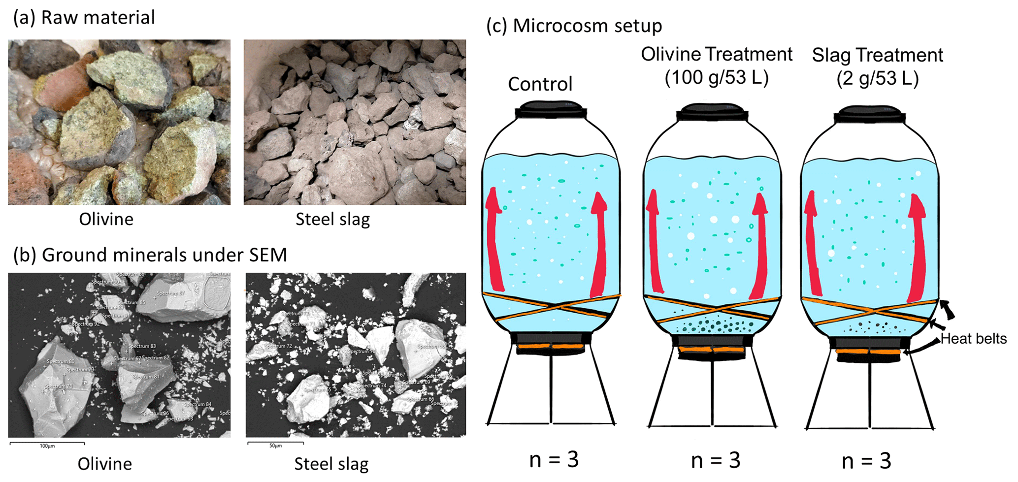
Figure 1 Experimental design and alkalinity sources. Panel (a) presents the raw materials used as alkalinity sources: olivine (left) and steel slag (right). Olivine and steel slag were originally larger than 20 mm. Panel (b) shows the ground minerals observed with a scanning electron microscope (SEM). Panel (c) outlines the microcosm setup: each microcosm enclosed ∼53 L of surface seawater with natural plankton communities. Olivine and steel slag treatments and the control were kept in a temperature-controlled room, and two heat belts were attached to the bottom of each microcosm to create convective circulation.

2 Methodology

2.1 Microcosm setup

We used nine 53 L transparent KegLand^® FermZilla conical unitank fermenters (polyethylene terephthalate) (Fig. 1) as microcosms to incubate natural plankton communities. All microcosms were prewashed with hydrochloric acid (10 % $v/v$) and rinsed five times with 18.2 MΩ Milli-Q water. Seawater with coastal plankton communities was collected at Battery Point (42.892° S, 147.337° E), Tasmania, within 2 h by lowering the microcosms into the ocean with a crane and filling them in a manner similar to a Niskin bottle, as described in detail in Ferderer et al. (2022). A sieve with a mesh size of 2 mm was attached to the top and bottom of the microcosms during filling to avoid the entrapment of large and patchily distributed organisms. The enclosed seawater weight was initially between 52.35 and 54.70 kg. After seawater collection, filled microcosms were immediately transported back to the Institute for Marine and Antarctic Studies (University of Tasmania) on a truck and transferred within 75 min into a temperature-controlled room set to 7.5–8 °C. Two heat belts were attached to the bottom of each microcosm to induce a convective mixing current (Ferderer et al., 2022). Seawater temperature inside the microcosms was about 13.5 °C due to the heating effects of the heat belts and was the same as the sampled region. Light-emitting diode (LED) light strips were used to provide an average light intensity of 236 µmol photons m⁻² s⁻¹ (ranging from 208 to 267 µmol photons m⁻² s⁻¹) with a daily light–dark cycle of 10 h (light) and 14 h (dark). The light intensity was the average light intensity in each microcosm measured with a LI-COR light meter at 0.15 m depth within the microcosm. Microcosms positioned in the temperature-controlled room were shuffled anti-clockwise every day to ensure similar light intensity for each microcosm throughout the experiment. Treatments were established 24 h after collecting the seawater. The total alkalinity released per amount of mineral powder added was much higher for the slag powder than the olivine powder in our preliminary test trials. Thus, three microcosms were enriched with 100 g of olivine powder, three microcosms were enriched with 2 g of steel slag powder, and the remaining three microcosms were left unperturbed and served as controls.

2.2 Preparation of olivine and steel slag powder

The olivine rocks were provided by Moyne Shire Council, who sourced the mineral from a quarry in Mortlake, Victoria, Australia. The basic oxygen slag (hereafter referred to as “slag”) was provided by Bradley Mansell, who sourced the material from Liberty Primary Steel Whyalla Steelworks in Whyalla, South Australia, Australia. Upon delivery, the olivine rocks were 40–80 mm in diameter, and slag aggregates were 20–50 mm in diameter. These were crushed to pieces that were smaller than 10 mm using a hydraulic crusher. The crushed material was further ground with a ring mill with a chrome milling pot. Afterwards, finely ground samples were sieved to get samples with a 150–250 µm grain size. The sieved olivine and slag grains were inspected with respect to their appearance and elemental composition using a Hitachi SU-70 analytical field emission scanning electron microscope (SEM) and energy-dispersive spectrometers (Central Science Laboratory – CSL, University of Tasmania). Grain size spectra were determined with a Sympatec QICPIC particle size analyzer LIXCELL (CSL, University of Tasmania).

2.3 Seawater sampling

Seawater was transferred with a peristaltic pump from the microcosms at a depth of about 0.15 m into 1 L acid-washed low-density polyethylene sampling bottles using an acid-washed silicon tube. Seawater in these bottles was then subsampled for dissolved trace metal samples, filtrations, fast-repetition-rate fluorometry (FRRf), and flow cytometry analysis. Samples for nutrients and total alkalinity (TA) were transferred using the same pump but through a silicone tube into 80 mL high-density polyethylene bottles. TA and macronutrient samples were filtered during this process through a 0.2 µm nylon filter attached to the silicone tube to remove all particles and organisms >0.2 µm.

2.4 Salinity, nutrients, carbonate chemistry, and trace metal analysis

Salinity was measured before and at the end of the experiment using a HACH HQ40d portable meter. The pH_T (total scale) and temperatures were measured daily (2–3 h after the onset of the light period) using a pH meter (914 pH/Conductometer Metrohm). We recorded voltages and temperature from the pH meter and calibrated the pH_T at the original temperature at the sampled time using the certified reference material (CRM) Tris buffer following the method described in SOP6a by Dickson et al. (2007). Briefly, the standard buffer's pH and voltage at different temperature gradients were recorded, and temperature vs. voltage polynomial regression data were generated for calculating calibrated pH values (pH_T) (refer to Eq. 3 in SOP6a of Dickson et al., 2007). The regression could then be used to obtain a CRM pH value for each temperature and to calibrate the pH measured in the microcosms to the total pH scale.

TA was sampled every 4 d. It was measured in duplicate using a Metrohm 862 Compact Titrosampler coupled with an Aquatrode Plus with a PT1000 temperature sensor following the SOP3b open-cell titration protocol described in Dickson et al. (2007). Filtered TA samples were stored at 8 °C for a maximum of 23 d before measurement. Titration curves were evaluated using the “calkulate” script within PyCO2SYS by Humphreys et al. (2022). The carbon chemistry equilibrium was calculated with the “seacarb” R package (Gattuso et al., 2024) from pH_T, TA, phosphate, silicate, temperature, and salinities using stoichiometric equilibrium constants from Lueker et al. (2000). Dissolved macronutrients were measured every second day using standard spectrophotometric methods developed by Hansen and Koroleff (1999) on the day the samples were taken from the microcosms.

Dissolved trace metal concentrations were measured four times during the experiment: a few hours before olivine and slag were added, a few hours after these minerals were added on day 2, near the middle of the experiment on day 13, and at the end of the experiment on day 22. A total of 60 mL of seawater was collected using an acid-washed 60 mL syringe, and the seawater was filtered through 25 mm diameter, 0.2 µm pore size polycarbonate filters. Unfortunately, we did not notice that 0.2 µm pore size nylon (acid-washed) filters were used during sampling on days 1 and 2, so we refiltered these seawater samples again using 0.2 µm pore size polycarbonate filters after 1 month. All seawater samples were diluted approximately 20-fold by weight using Milli-Q water (18.2 MΩ cm grade) and acidified using 1 % ultrapure HCl. These samples were analyzed using sector field inductively coupled plasma mass spectrometry (SF-ICP-MS) employing multiple resolution settings to overcome major spectral interferences. Due to the presence of abundant major metal ions in our samples, such as Na and Mg, natural open-ocean seawater from the Southern Ocean with very low trace metal concentrations was diluted 20 times with Milli-Q water and used as a representative blank. The same Southern Ocean seawater was enriched with different gradients of trace metal standards to calculate the samples' trace metal concentrations. A total of 5 of the 36 samples had abnormal trace metal concentrations, and 2 of them were from day 1. We considered values as outliers using the interquartile range (IQR) criterion on pre-addition data, and if values are more than 10 times higher than replicates, they are also considered to be outliers. These samples containing outliers were excluded from the data analysis (Table S1 in the Supplement). The major likely source of these metal contaminations is sampling in the temperature-controlled room, where precautions were insufficiently implemented.

2.5 Particulate matter and plankton community analysis

Chlorophyll a was sampled every second day by filtering the seawater through glass fiber filters (GF/F, 25 mm diameter, 0.7 µm pore size), and filters were stored in 15 mL polypropylene tubes wrapped with aluminum foil and stored at −80 °C for 50–70 d before measurement. Each filter was immersed in 10 mL of 100 % methanol for 18–20 h to extract chlorophyll from phytoplankton, and these samples were analyzed on a Turner fluorometer (Model 10-AU) following the method described by Evans et al. (1987).

Phytoplankton flow cytometry samples were fixed with 40 µL of a mixture of formaldehyde and hexamine (18 %:10 % $v/w$) added to 1400 µL of seawater sample. All bacteria samples (700 µL) were fixed with 14 µL of glutaraldehyde (electron-microscope grade, 25 %). After mixing samples with fixatives, samples were stored for 25 min at 10 °C, flash-frozen in liquid nitrogen, and stored at −80 °C until measurement 83–86 d later. Directly before the measurement, samples were thawed at 37 °C. Bacteria samples were stained with SYBR Green I (diluted in dimethylsulfoxide) at a final ratio of 1:10 000 (SYBR Green I : sample).

A Cytek Aurora flow cytometer (Cytek Biosciences) was used to quantify the abundance of fluorescing particles such as phytoplankton or stained bacteria. Phytoplankton groups were distinguished based on their fluorescence signal intensity of different laser excitation/emission wavelength combinations and forward scatter (FSC). The yellow–green laser (center wavelength: 577 nm), in combination with FSC signal strength, was used to separate cyanobacteria and cryptophytes from other phytoplankton. The violet laser (center wavelength: 664 nm), in combination with FSC, was used to distinguish picoeukaryotes, nanoeukaryotes, and microphytoplankton. The blue laser (center wavelength: 508 nm), in combination with FSC, was used to distinguish bacteria from other living (i.e., DNA-containing) particles (Fig. S1 in the Supplement).

The biovolume of each classified flow cytometry phytoplankton type was calculated using the following equation:

$$\begin{array}{}\text{(4)}& \mathrm{biovolume}=\text{cell\hspace{0.17em} number\hspace{0.17em} count}\times {\left({\displaystyle \frac{\mathrm{FSC}}{\mathrm{10}\mathrm{248}}}\right)}^{\mathrm{2.14}},\end{array}$$

where biovolume is the biovolume of the phytoplankton (µm³), cell number is the cell count per milliliter of sample, and FSC is the forward-scatter signal value from the flow cytometry. This equation is calculated based on the relationship between biovolume and FSC for different phytoplankton species (Selfe, 2022). The biovolume of each phytoplankton type was then divided by the total biovolume of all phytoplankton types to calculate the biovolume proportion of each phytoplankton type (biovolume prop.). This derived value was used to estimate the phytoplankton composition in each microcosm.

Phytoplankton photosynthetic performance was estimated from the rapid light curves measured with an FRRf (FastOcean sensor FRRf3, Chelsea Instruments Group) every second day following the protocol adapted from Schallenberg et al. (2020). Samples were kept in the dark for 20 min before the measurement and then added to the FRR fluorometry cuvette, which was temperature-controlled at 13.5 °C. Filtered natural seawater was used for blank correction. A channel with three light wavelengths (450, 530, and 624 nm) was used in each acquisition sequence. At least 10 acquisitions were measured for each sample. The maximum electron transport rate (ETR_max), initial slope of the rapid light curve (α), and the light-saturation parameter (E_k) were calculated using the equation described by Platt et al. (1980) without photoinhibition:

$$\begin{array}{}\text{(5)}& \mathrm{ETR}={\mathrm{ETR}}_{\max }\left[\mathrm{1}-e^{-\frac{\mathit{\alpha }E}{{\mathrm{ETR}}_{\max }}}\right].\end{array}$$

These parameters and the maximum quantum yield of photosystem II ($F_v/F_m$) were used to compare the photosynthetic performance of the phytoplankton communities in different microcosms.

Seawater was sampled before the treatment and at the end of the experiment for particulate trace metal concentrations. Samples of 100 mL were filtered through an acid-cleaned polycarbonate filter (25 mm diameter, 0.8 µm pore size) and placed in an acid-cleaned polypropylene filter holder in a trace-metal-clean laminar flow bench. The filters were washed with EDTA–oxalate reagent (1.4 mL) twice (8 min total) and rinsed with chelexed NaCl solution (0.6 mol L⁻¹ with 2.38 mmol L⁻¹ of HCO${}_{\mathrm{3}}^{-}$, pH =8.2) 10 times (1.5 mL aliquots) (Tovar-Sanchez et al., 2003; Tang and Morel, 2006). Filters were stored in acid-washed well plates at −20 °C before analysis. The digestion process followed the method reported by Bowie et al. (2010). Briefly, all samples and triplicate certified reference material plankton standards (50 mg per vial) were digested in a mixture of strong ultrapure acids (750 µL of 12 mol L⁻¹ HCl, 250 µL of 40 % HF, 250 µL of 14 mol L⁻¹ HNO₃) in 15 mL Teflon perfluoroalkoxy vials on a 95 °C hot plate for 12 h in a fume hood. They were then dry evaporated for 4 h and resuspended in 10 % $v/v$ ultrapure HNO₃. All prepared solutions had indium as the internal standard added to a final concentration of 10 µg L⁻¹. Three premixed multielement standard solutions (MISA) were prepared as external calibration standards.

Particulate organic carbon (POC) was sampled by filtering 100 mL of seawater from each microcosm. Glass fiber filters (Whatman GF/F, 13 mm diameter, 0.7 µm pore size) were pre-combusted at 400 °C for 6 h. Filters were stored at −20°C before measurement. Samples were treated via fuming with 2N HCl to remove carbonates overnight and dried in the oven for 4 h. Finally, filters were folded into silver cups and stored in a desiccator until analysis. Samples were analyzed for carbon with a Thermo Finnigan FlashEA 1112 Elemental Analyzer (CSL, University of Tasmania).

Biogenic silica (BSi) concentrations were analyzed every 4 d by filtering 100 mL of seawater from each microcosm. Mixed cellulose ester (MCE) membrane filters (25 mm diameter, 0.8 µm pore size) were used for BSi samples. BSi filters were placed in a plastic Petri dish and stored at −20 °C before measurement. Filters were processed using the hot NaOH digestion method of Nelson et al. (1989). The final solution was measured using the same process as the dissolved silicate (see Sect. 2.4).

A self-made plastic zooplankton net (20 mm height and 15 mm width) with a 210 µm mesh size was acid-washed first and then used to collect zooplankton from microcosms before mineral addition on day 2, near the middle (day 13), and at the end of the experiment (day 23). Samples were stored in 10 % formalin seawater solutions and kept at room temperature until measurements. Zooplankton were quantified and identified under a Leica M165C microscope fitted with a Canon 5D camera. The number of zooplankton from one mini-trawl in each collection was converted to the unit of individuals per liter and used for data analysis. The diversity of zooplankton communities was estimated with the Shannon diversity index (H), calculated as follows:

$$\begin{array}{}\text{(6)}& H=-\sum (\mathrm{pi}\times \ln (\mathrm{pi}\left)\right),\end{array}$$

where pi is the proportion of the entire zooplankton community made up of individual species abundance and ln is the natural logarithm.

2.6 Statistic analysis

R studio was used for data analyses. Generalized additive models (GAMs) from the “mgcv” package were fitted to the data to predict the changes over time. The GAMs all shared the same equations:

$$\begin{array}{}\text{(7)}& Y=s\left(\mathrm{Day}\right),\end{array}$$

in which Y presents the dependent variable and s(Day) is the smooth term of the day of the experiment. Another GAM was used to detect significant differences between treatments and the control:

$$\begin{array}{}\text{(8)}& Y=\mathrm{Treatment}+s\left(\mathrm{Day}\right)+s(\mathrm{Day},\mathrm{by}=\mathrm{oTreatment})\end{array}$$

In this equation, the variable “Treatment” includes three conditions – “Control”, “Slag”, and “Olivine” – while “oTreatment” is the ordered factor of the variable Treatment that allowed us to compare the GAMs' smooth terms from different treatments and the control (Simpson, 2017).

When comparing GAMs, “P-means” represents the p value obtained from comparing two GAMs, such as the control and the olivine treatment. If P-means is below 0.05, it indicates that the mean values of the two GAMs exhibit significant differences over the course of the experiment. Conversely, if P-means is equal to or greater than 0.05, it suggests that the two GAMs have similar mean values. In contrast, “P-smooths” represents the p value derived from comparing the smooth terms of two GAMs. If P-smooths is below 0.05, it indicates that the two GAMs demonstrate significantly different trends in their change over time.

For the analysis of trace metal concentrations and zooplankton abundance, generalized linear models (GLMs) from the “stats” package were fitted to the data to determine significant differences between treatments and the control. The selection of specific GLMs was based on the distribution of the raw data. One GLM equation is as follows:

$$\begin{array}{}\text{(9)}& Y=\mathrm{Treatment}+{\displaystyle \frac{\mathrm{Day}}{\mathrm{22}}}+{\left({\displaystyle \frac{\mathrm{Day}}{\mathrm{22}}}\right)}^{\mathrm{2}}.\end{array}$$

Here, Y represents the measured parameter (abundance of a zooplankton species and dissolved trace metal concentrations), treatment is the conditions (Control, Slag, and Olivine), and Day represents the day of the experiment. The other GLM equation is as follows:

$$\begin{array}{}\text{(10)}& Y=\mathrm{Treatment}+\mathrm{Day}.\end{array}$$

This expression was employed for particulate trace metal data and the Shannon diversity index. To compare the contribution of the three treatments on the measured parameters, Tukey's significant difference test was conducted on the GLMs using the “glht” function.

3 Results

3.1 Elemental composition and grain size of the finely ground minerals

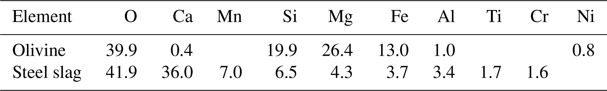
SEM analysis revealed the approximate elemental composition of olivine and slag powder (Table 1). Based on this analysis the olivine composition resembles the Mg-rich olivine mineral “forsterite” (Mg₂SiO₄). The particle size spectrum of olivine powder is shown in detail in Fig. S2. Roughly 69 % of the olivine particles, when measured by volume, fell within the diameter range of 35–300 µm. Additionally, SEM analysis revealed high levels of Ca and O in the slag, indicative of the considerable Ca(OH)₂ and CaO content of the powder (Table 1; please note that H cannot be measured with the applied method). The particle size measurement (Fig. S2) showed that 78 % of the ground slag particles were between 35 and 300 µm.

Table 1 The weight percentage of elements from two minerals (unit: wt %).

3.2 Physical and chemical conditions over the course of the experiment

On day 2 of the experiment, when olivine particles were introduced into the microcosms, the smallest fraction of the powder remained suspended, causing the seawater to become highly turbid for several days. The resulting milky appearance of the seawater eventually faded over a period of approximately 5 d, and by day 5, the turbidity had visually become like the slag treatment and the control. This effect was not anticipated, and as a result, we decided to investigate its impact on light intensity. To do so, a test was conducted after the main experiment in which olivine powder was added to a microcosm identical to those used in the experiment, and light intensity was measured daily at a depth of 0.15 m. The results showed that the addition of olivine caused an initial reduction in light intensity of 18.5 % at 15 min after addition, which declined to 7.4 %, 3.7 %, 3.7 %, and 0 % after 1, 2, 3, and 4 d, respectively. These findings indicate that olivine additions can significantly affect the light environment in the microcosms, whereas no such effect was observed in the slag treatment.

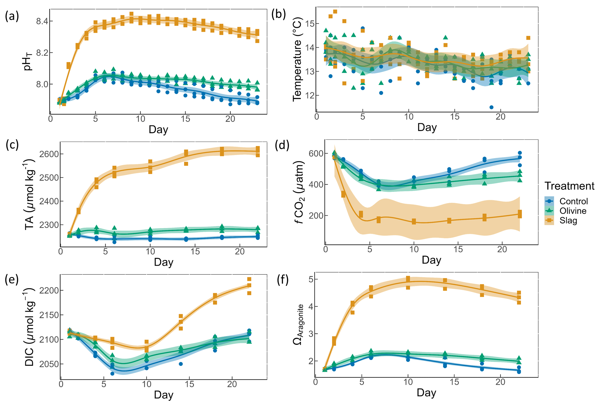
Figure 2 Carbonate chemistry conditions. The temporal development of (a) pH_T, (b) temperature, (c) total alkalinity (TA), (d) CO₂ fugacity (fCO₂) computed at in situ temperature and atmospheric pressure, (e) dissolved inorganic carbon (DIC), and (f) aragonite saturation state (Ω_aragonite). The dots represent the raw data (n=3 for each treatment per sampling time), and the fitted curve is the generalized additive model (GAM). The shading represents the 95 % confidence interval of the fitted GAM.

The pH_T of all microcosms increased from day 1 to day 5 (Fig. 2a). This was due to photosynthetic CO₂ drawdown in the control or photosynthetic CO₂ drawdown in combination with alkalinity release from minerals in the treatments. During the peak of the bloom, pH_T was 8.037±0.010 in the control (average values ± standard error), 8.054±0.014 in the olivine treatment, and 8.411±0.015 in the slag treatment. The pH_T was significantly higher in the slag than the olivine treatment and the control throughout the experiment (control and olivine pH_T were not significantly different). The pH_T on day 23 of the control, olivine, and slag treatments were 7.893±0.012, 7.978±0.015, and 8.309±0.019, respectively. The temperature inside of the microcosms varied between replicates, which may have added noise in the biological response data. However, on average, there was no statistically significant difference between the control and treatments during the experiment.

In our data analysis, all of the fitted GAMs from the treatments and the control exhibited significant differences in pH_T from each other, as evidenced by the p values of both P-means and P-smooths being smaller than 0.001. For detailed results of the GAM p values, please refer to Table S2.

TA increased marginally from 2255±2 to 2262±13 µmol kg⁻¹ within the first 6 d after olivine addition, while it increased more substantially from 2259±1 to 2522±11 µmol kg⁻¹ in the same time span in the slag treatment (Fig. 2c). The TA in the control decreased from 2261±2 to 2240±7 µmol kg⁻¹ from day 1 to day 6 but remained stable thereafter. The TA reached 2279±6 µmol kg⁻¹ in the olivine treatment and 2611±9 µmol kg⁻¹ in the slag treatment on day 22. The slag treatment reached a significantly higher TA than the olivine treatment and the control (P-smooths <0.001). The mean TA from the GAM in the olivine treatment was higher than the control (P-means <0.001).

The CO₂ fugacity (fCO₂) computed at in situ temperature and atmospheric pressure decreased continuously in the first 6 d in all microcosms (Fig. 2d). Then, it increased again in the control and olivine treatments while remaining lower in the slag treatment (P-means and P-smooths ≤0.001 between either treatment or the control). DIC (Fig. 2e) and the aragonite saturation state (Ω_aragonite; Fig. 2f) revealed a similar trend over the course of the experiment in the control and the olivine treatment. In contrast, the slag treatment had higher DIC and Ω_aragonite values throughout the experiment (P-means <0.001).

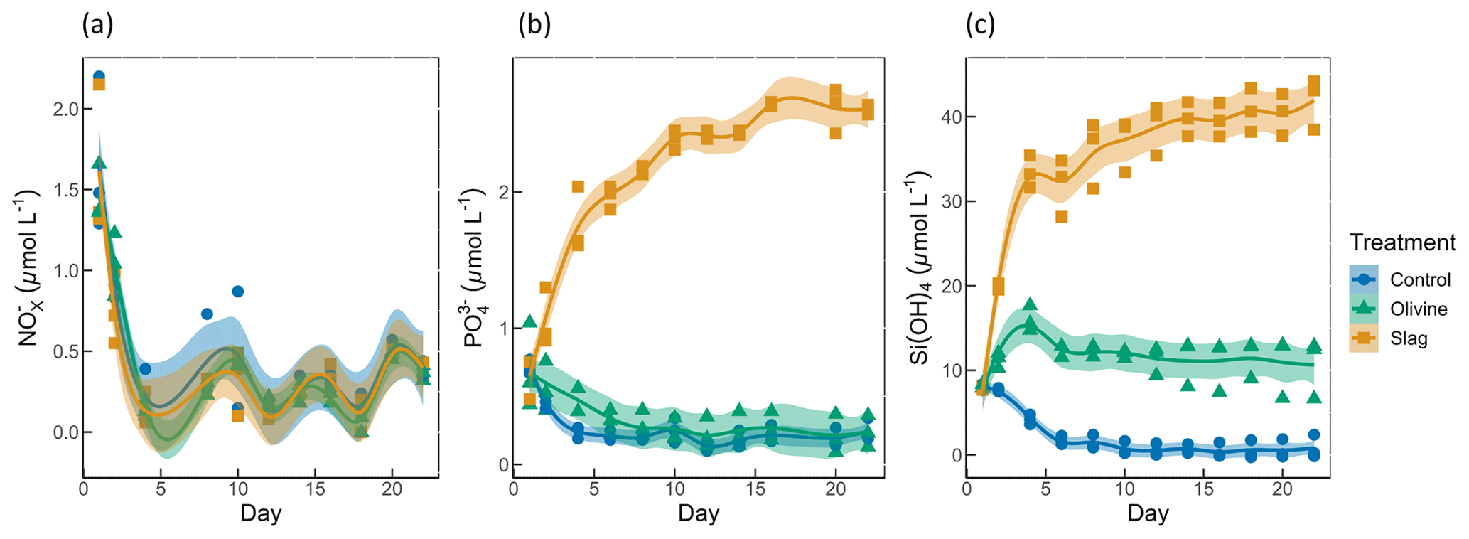
Figure 3 Macronutrient concentrations over the course of the study: (a) nitrate and nitrite concentrations; (b) phosphate concentrations; (c) silicic acid concentrations. The dots represent the raw data (n=3 for each treatment per collection), and the fitted curve is the generalized additive model.

Initial nitrate and nitrite (NO${}_x^{-}$), phosphate (PO${}_{\mathrm{4}}^{\mathrm{3}-}$), and silicic acid (Si(OH)₄) concentrations were 1.58±0.12, 0.69±0.59, and 8.04±0.10 µmol L⁻¹, respectively (Fig. 3). NO${}_x^{-}$ declined rapidly in all microcosms once the experiment had commenced (to values below 0.5 µmol L⁻¹), and no significant difference was detected between treatments and control (P-smooths >0.05; Fig. 3a). In both the olivine treatment and the control, the PO${}_{\mathrm{4}}^{\mathrm{3}-}$ concentration decreased in the first 6 d (Fig. 3b). In the slag treatment, PO${}_{\mathrm{4}}^{\mathrm{3}-}$ increased to a maximum of 2.65±0.01 µmol L⁻¹, which was significantly higher than in the olivine treatment and the control (P-means <0.001). The Si(OH)₄ concentration increased to a maximum of 15.99±0.87 µmol L⁻¹ in the olivine treatment, increased to a maximum of 41.92±1.75 µmol L⁻¹ in the slag treatment, but decreased below the detection limit in the control (Fig. 3c). Significant differences were observed in the development of Si(OH)₄ between all treatments and the control (Table S2).

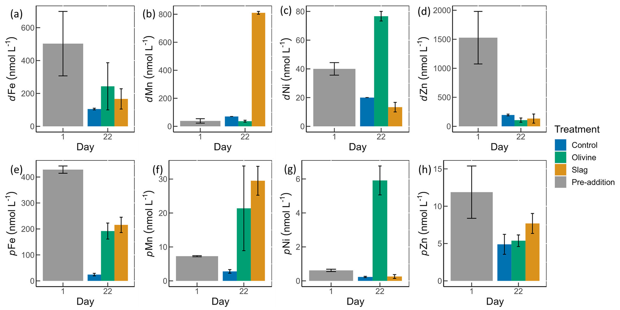
Figure 4 Dissolved and particulate trace metal concentrations in microcosm seawater. Panels (a)–(d) show dissolved trace metal concentrations, while panels (e)–(h) present total particulate trace metal concentrations. The error bars represent the standard error from measured samples. The pre-addition data shown in panels (a)–(d) represent the average of seven microcosms before the addition of slag or olivine. The data for the control on day 22 in panels (a)–(d) and for the pre-addition on day 1 in panels (e)–(h) were based on two of three microcosm replicates. The remaining data were based on all three microcosm replicates.

The dissolved trace metal concentrations measured from microcosms are presented in Fig. S3. While the mass of olivine added to the microcosms was 50-fold greater than that of steel slag (100 g vs. 2 g), it is noteworthy that the variation in dissolved trace metal concentrations between the two treatments was much smaller than 50-fold. After 21 d of experiment, the treatments showed an increase in dissolved Al concentrations from 920±286 to 970±228 nmol L⁻¹ in the olivine treatment and from 920±286 to 1093±77 nmol L⁻¹ in the slag treatment, while dissolved Al decreased to 230±10 nmol L⁻¹ in the control (Fig. S3). The fitted GLMs were compared, and the p value revealed how much influence a treatment had on the dissolved metal concentrations (Table S3). The results indicate that the slag and olivine additions led to significantly higher Al concentrations than in the control (p values <0.05), but no significant difference was found between the two treatments (p value =0.189). The Cu concentration in the olivine on day 22 was significantly higher than the slag treatment and the control (p value <0.05; Fig. S3). The addition of olivine and slag released some dissolved Fe; however, overall, the concentration of Fe did not differ significantly between treatments (Fig. 4a, Table S3). The slag released a substantial amount of dissolved Mn (maximum 810±10 nmol L⁻¹ on day 22; Fig. 4b), leading to significantly higher concentrations than in the olivine treatment and the control (p values <0.001). A significant amount of dissolved Ni (maximum 77±3 nmol L⁻¹ on day 22) was released from the olivine powder (p values <0.001; Fig. 4c). The initial concentration of dissolved Zn in seawater was much higher than on day 22 in all microcosms, and no significant difference in Zn concentrations was found between the treatments and the control.

Particulate concentrations of some trace metals also differed between treatments. The total particulate Fe decreased in all microcosms on day 22 compared with the pre-addition level, but both mineral addition treatments had higher particulate Fe concentrations than the control (Fig. 4e). The addition of slag elevated particulate Mn concentrations to a level higher than the pre-addition and the control on day 22 (Fig. 4f), while the addition of olivine increased the particulate Ni concentrations to a level higher than the slag, the control, and the pre-addition (Fig. 4g). The particulate Zn concentrations generally decreased by the end of the experiment (Fig. 4h), and no significant differences were found between the treatments and the control.

The POC concentrations on day 1 and day 22 from all microcosms were very similar, 10.99±0.58 and 11.03±0.41 µmol L⁻¹, respectively (Fig. S4); thus, the metal : POC ratio results were consistent with the particulate trace metal results (Fig. 4e–h). In general, the non-surface metal : POC ratios are positively correlated with the total metal : POC ratios (Fig. S5). The ratio of non-surface to total particulate trace metal concentrations is summarized in Table S5. Both non-surface and total Fe concentrations decreased in microcosms on day 22 compared with the pre-addition level. Fe : POC ratios were significantly higher in the treatments than in the control on day 22 (p values <0.05; Table S3), and there was no significant difference between mineral addition treatments. The non-surface to total Fe : POC ratios were >0.94 in all microcosms on both day 1 and day 22. The total and non-surface Mn : POC ratio was the highest in the slag treatment. These ratios were higher than the pre-addition level and the control at the end of the experiment. The total particulate Ni concentrations in the olivine treatment were significantly higher than before olivine addition. The olivine treatment led to a >22-fold higher Ni : POC ratio compared with the other two treatments (p value <0.001).

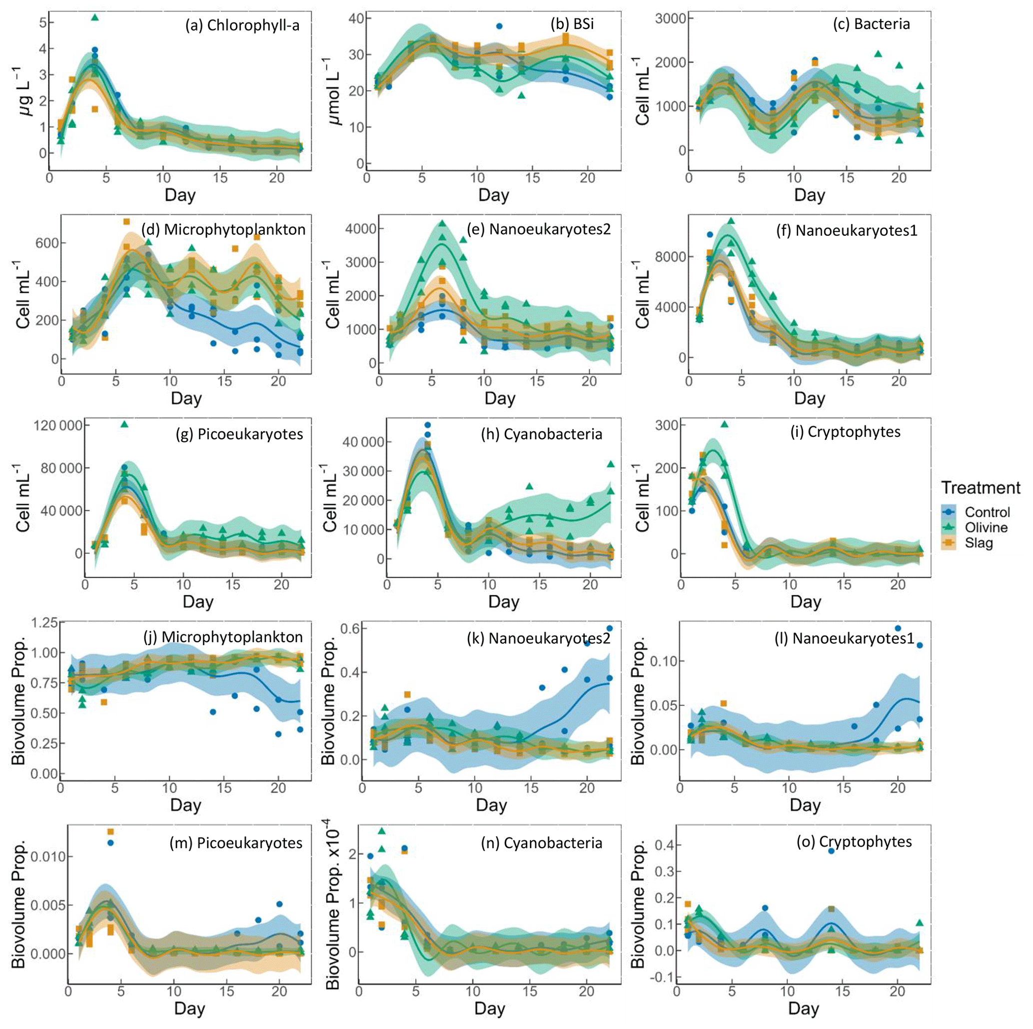
Figure 5 Temporal development of the chlorophyll-a (chl-a) concentration, BSi, and different eukaryotic and bacterial plankton groups as determined with flow cytometry. The panels show the following: (a) chlorophyll a; (b) BSi; cell concentrations of (c) heterotrophic bacteria, (d) microphytoplankton, (e) nanoeukaryotes2, (f) nanoeukaryotes1 (g) picoeukaryotes, (h) cyanobacteria, and (i) cryptophytes; and biovolume proportion of (j) microphytoplankton, (k) nanoeukaryotes2, (l) nanoeukaryotes1 (m) picoeukaryotes, (n) cyanobacteria, and (o) cryptophytes. The figure data points represent the raw data, and the fitted curve is the generalized additive model. The shaded area represents the 95 % confidence interval.

3.3 Development and physiology of the plankton community

The chl-a concentration in all microcosms increased from 1 to 3–4 µg L⁻¹ from day 1 to day 4 (Fig. 5a). The chl-a concentration then decreased rapidly from day 4 to day 8 and continued to decrease, although more slowly, to <0.3 µg L⁻¹ until the end of the experiment. The GAMs of chl a did not show any difference between treatments and the control (both P-means and P-smooths >0.05; see Table S2).

The BSi concentration increased from day 1 to day 6 in all microcosms (Fig. 5b). In the olivine treatments, BSi concentrations decreased slightly after the peak until day 12 but then increased again. In the slag treatment, BSi concentrations remained relatively stable after the initial phytoplankton bloom. In contrast, the BSi concentration decreased continuously in the control after the initial peak. Olivine particles suspended in seawater after the mineral addition (see Sect. 3.2) partially ended up on BSi filters during filtration. This led to extremely high BSi measurements on days 2 and 4 that were removed from Fig. 5b. Without these outliers, the mean of the fitted BSi GAM in the olivine treatment was lower than the control and the slag treatment (Table S2), and the slag treatment had the highest average BSi over the course of the experiment. Overall, the BSi trends in the two treatments were similar (P-smooths =0.269), and both were significantly different from the control (P-smooths <0.05).

The development of the phytoplankton community composition showed significant differences between the treatments and the control. In general, most phytoplankton groups exhibited similar patterns to chl a, with peak cell numbers occurring on day 4 (Fig. 5f, g, h, i), apart from microphytoplankton and nanoeukaryotes2, which had the peak delayed for 1–2 d (Fig. 5d, e). Please be aware that flow cytometers may not capture some large and chain-forming phytoplankton. After reaching peak values during the bloom, phytoplankton abundance generally decreased steadily. Microphytoplankton displayed similar trends to the results for BSi. Before day 10, all microcosms had similar microphytoplankton abundances (Fig. 5d). However, in the control, microphytoplankton abundance declined continuously and at a faster rate compared with the two treatments (P-smooths values <0.03). From day 2 to day 6, the abundance of nanoeukaryotes1, nanoeukaryotes2, picoeukaryotes, and cryophytes was higher in the olivine treatment compared with the slag treatment and the control. After day 8, their abundance in the olivine treatment decreased to a similar level to the slag treatment and the control. Notably, there were few significant differences observed between the slag treatment and the control in terms of the abundances of nanoeukaryotes1, nanoeukaryotes2, picoeukaryotes, cyanobacteria, and cryptophytes throughout the experiment. In the olivine treatment, cyanobacteria experienced a second bloom after day 10, which was significantly different from the other two groups (P-smooths <0.01). Heterotrophic bacteria exhibited an increase and decline pattern following the phytoplankton bloom until day 8 (Fig. 5c). Subsequently, bacterial abundance increased again, reaching a second peak during days 12–14, followed by a decline until the end of the experiment. The decline in bacterial abundance was slower in the olivine treatment, although no significant differences were detected between treatments (Table S2).

Among all of the microcosms, microphytoplankton consistently accounted for the largest proportion of biovolume. From the perspective of biovolume proportion, the mineral addition mainly influenced the microphytoplankton and nanoeukaryotes. The control had similar phytoplankton biovolume distribution as the treatments from day 1 to day 15, but the proportion of microphytoplankton biovolume subsequently decreased to a level significantly lower than that of the treatments. In the control treatment, the proportion of nanoeukaryotes' biovolume increased as the proportion of microphytoplankton decreased. The biovolume of picoeukaryotes, cyanobacteria, and cryptophytes increased during the phytoplankton bloom and then decreased drastically after the bloom. There were no significant differences in the biovolume proportion observed for picoeukaryotes, cyanobacteria, and cryptophytes between the treatments and the control.

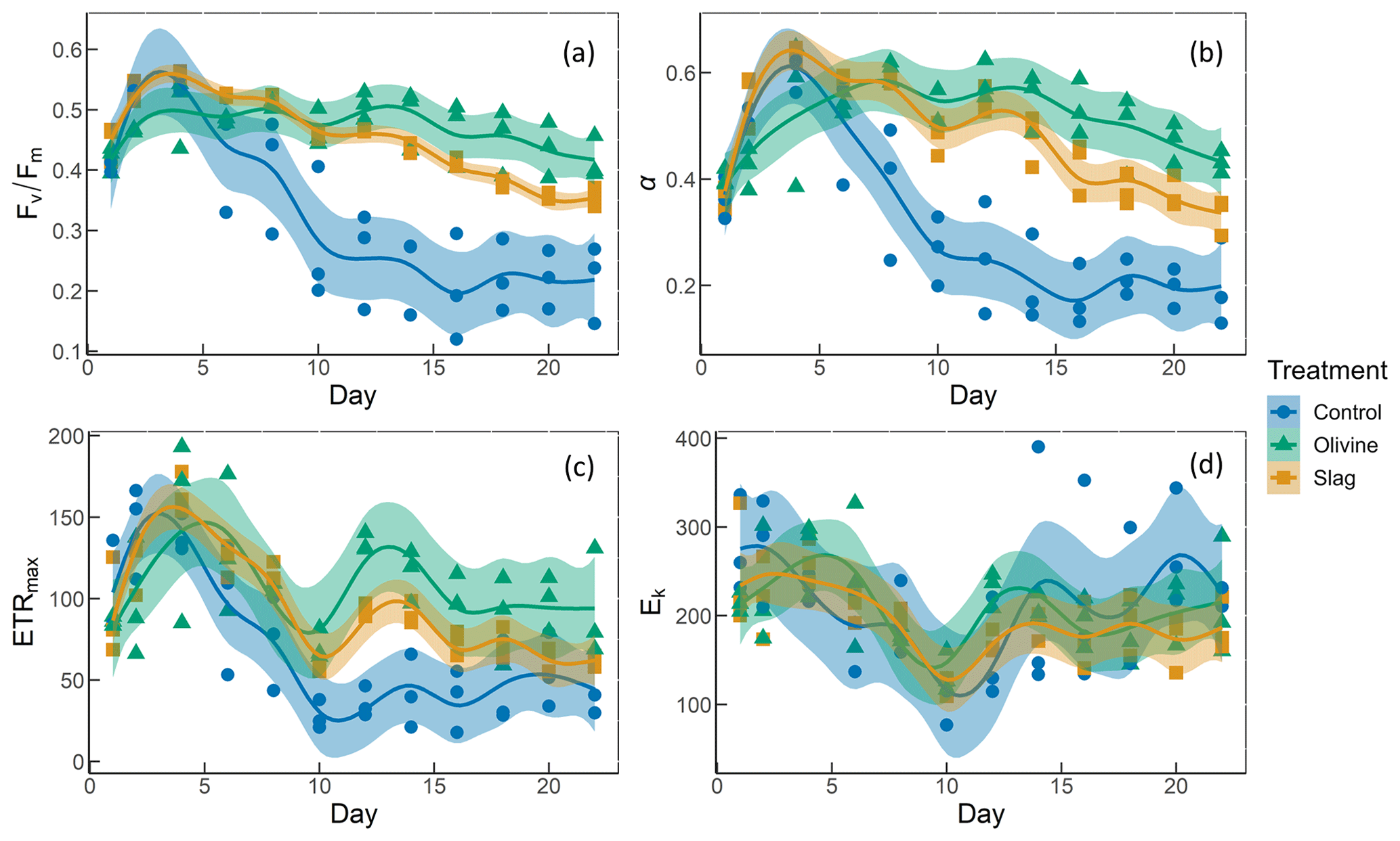
Figure 6 The photosynthetic performance of the phytoplankton community. The panels show the following: (a) $F_v/F_m$, the maximum quantum yield of photosystem II; (b) α, the initial slope of the rapid light curves; (c) ETR_max, the maximum electron transport rate; and (d) E_k, the light-saturation parameter (unit: µmol photons m⁻² s⁻¹).

The temporal development of $F_v/F_m$, α, ETR_max, and E_k is illustrated in Fig. 6. The $F_v/F_m$ values of the phytoplankton community were approximately 0.42±0.01 and increased to levels >0.5 during the peak of the phytoplankton bloom on day 4 (Fig. 6a). Following the bloom, $F_v/F_m$ values dropped below 0.3 in the control. However, the decline in $F_v/F_m$ after the bloom was less pronounced in the two mineral addition treatments, with the olivine treatment maintaining higher $F_v/F_m$ values than the slag treatment (P-smooths <0.05). At the end of the experiment, $F_v/F_m$ was 0.22±0.04 in the control, 0.35±0.01 in the slag treatment, and 0.42±0.02 in the olivine treatment. The temporal development of α aligned with the patterns observed for $F_v/F_m$ (cf. Fig. 6a and b). The maximum values of ETR_max were observed on day 4 in the control and the slag treatment, while the maximum value occurred on day 5 in the olivine treatment (Fig. 6c). Subsequently, ETR_max continuously decreased until day 10 and then stabilized until the end of the experiment. However, ETR_max exhibited a subsequent increase in the mineral treatments around day 12. The ETR_max values were higher in the mineral treatments compared with the control group (P-means <0.001; Table S2). The parameter E_k decreased from 246±17 µmol photons m⁻² s⁻¹ on day 1 to 121±7 µmol photons m⁻² s⁻¹ on day 10, and it then increased again to approximately 200 µmol photons m⁻² s⁻¹ by the end of the experiment (Fig. 6d). The change in E_k did not exhibit significant differences between the treatments and the control (both P-means and P-smooths >0.05).

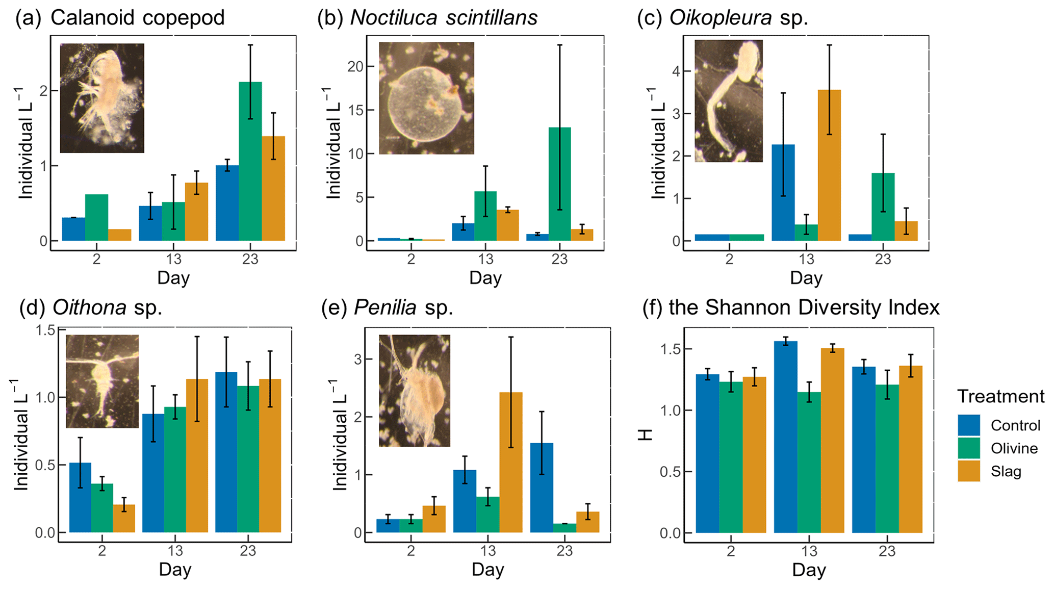
Figure 7 The dominant zooplankton abundance and community diversity from different treatments. Abundance of dominant zooplankton in microcosms for (a) calanoid copepod, (b) Noctiluca scintillans, (c) Oikopleura sp., (d) Oithona sp., and (e) Penilia sp. as well as (f) the Shannon diversity index (H) of different treatments and the control. Error bars represent the standard error calculated from three microcosm replicates. Photographs of each zooplankton group are shown on the corresponding graphs.

A total of 13 zooplankton taxonomic groups were identified in the microcosms. The dominant taxa were the appendicularian Oikopleura sp., the cyclopoid copepod Oithona sp., the cladoceran Penilia sp., the heterotrophic dinoflagellate Noctiluca scintillans, and several calanoid copepods, including Acartia sp., Paracalanus sp., and Gladioferens sp. The larvae and eggs of Oikopleura, Penilia, and the copepod were also observed under the microscope. In general, higher zooplankton numbers were observed after the bloom on day 13 (Fig. 7). The abundance of calanoid copepods and Oithona sp. increased after day 2 (Fig. 7a, d), and there was no significant difference between treatments and the control (p values >0.05; Table S4). The abundance of N. scintillans increased significantly more in the olivine treatment than in the control and the slag treatment, with the highest abundance of 13±9 individuals L⁻¹ observed in the olivine treatment on the last day (Fig. 7b). The abundance of Oikopleura in the control and the slag treatment was higher than the olivine treatment on day 13 but was higher in the olivine treatment on day 22 (Fig. 7c). A higher abundance of Penilia sp. was found in the slag treatment on day 13 and in the control on day 23 (Fig. 7e). Due to the patchy distribution of zooplankton, these data have large standard errors, and only the differences in the numbers of N. scintillans in the olivine treatment were statistically significantly different from the slag treatment and the control (p value <0.05; Table S4).

Considering the control and the slag treatment, the Shannon diversity index (H) increased from day 2 to day 13 and declined on day 23, while H was lower on day 13 than on day 2 and day 23 in the olivine treatment (Fig. 7f). The GLMs revealed that the olivine treatment had significantly lower H on day 13 than the control and the slag treatment (p values <0.001). There were no significant differences in H between the control and the slag treatment (Table S4). The addition of olivine decreased the zooplankton community's diversity. This is mainly driven by distinct trends observed in the abundance of Oikopleura sp., Penilia sp., and N. scintillans (Fig. 7).

4 Discussion

4.1 CO₂ removal potential of slag and olivine

The slag powder used here (i.e., basic oxygen slag from Whyalla, Australia) created significantly higher CO₂ removal potential than the olivine powder used here (i.e., olivine from Mortlake, Australia) over the course of the study. Ca(OH)₂ and CaO in slag and Mg₂SiO₄ in olivine are likely to be the main functional minerals driving the measured alkalinity enhancement. TA increased by 361 µmol kg⁻¹ in the slag treatment, whereas it increased by only 29 µmol kg⁻¹ in the olivine treatment, equivalent to a potential 14.7 % and 0.9 % increase in marine inorganic carbon, respectively, within 3 weeks of their application. When normalizing these alkalinity increases to the same material weight, 1 g of slag would release 9626 µmol TA, whereas 1 g of olivine would release 16 µmol TA. Thus, over 3 weeks of experimental incubation, slag is ∼600-fold more efficient at releasing alkalinity for particles of this size class (note that the particle size spectra of olivine and slag were similar but not identical; Fig. S1). We can also use these values to roughly estimate how much CO₂ these two minerals could potentially sequester. A total of 1 mol of alkalinity from olivine and slag can sequester approximately 0.85 mol of CO₂. Thus, 1 metric ton of slag and olivine powder, as used here, could sequester 360 and 0.6 kg of CO₂, respectively, within 3 weeks. Please note, however, that the amount of olivine added to the experiments (1.9 g L⁻¹) contains substantially more alkalinity in the solid phase than the slag and that this alkalinity could be released over longer timescales so that the CDR efficiency of olivine could increase more substantially than slag over time. Furthermore, it is likely that the optimization of the particle size and the application method may lead to higher efficiencies of the slag but especially of the olivine with its inherently slower dissolution rate. Last, it needs to be emphasized that other types or sources of slag and olivine may have slightly different compositions; therefore, the CDR potentials estimated here as well as the associated environmental implications discussed below may vary accordingly.

4.2 Environmental implications of slag and olivine additions

The amount of olivine and slag powder added to the treatments differed significantly (100 g of olivine powder was added, whereas only 2 g of slag powder was added to the 53 L microcosms). Our rationale for these different mass additions was to yield somewhat similar amounts of detectable alkalinity enhancement in the dissolved phase, as we already knew (from tests before the experiment) that slag elevates alkalinity faster than olivine. However, olivine was less efficient at releasing alkalinity than we had anticipated so that even a 50-fold higher addition of olivine (with respect to mass) did not compensate for this difference. As such, our experiments are associated with an “apples and oranges” issue in that our perturbation with minerals and associated OAE differs. To account for this, the following discussion mainly relates the observed environmental effects to the alkalinity enhancement achieved over the course of the study.

4.2.1 OAE effects on phytoplankton physiology and community

Previous research has hypothesized that OAE-induced changes in seawater carbonate chemistry could delay phytoplankton bloom formation due to reductions in the seawater partial pressure of CO₂ (pCO₂) in the aftermath of an OAE deployment (Bach et al., 2019). The buildup of the chlorophyll-a concentration as observed here was indistinguishable between treatments and the control, suggesting no effect of slag- or olivine-based OAE on phytoplankton bloom dynamics under these experimental settings. A lack of bloom delay due to carbonate chemistry is unsurprising for the olivine treatment, where the release of alkalinity was small (29 µmol kg⁻¹ alkalinity release), but it was somewhat more surprising in the slag treatment, where alkalinity was quite rapidly increased by 361 µmol kg⁻¹. However, the release was still lower than in a very similar study by Ferderer et al. (2022), where alkalinity was increased by 500 µmol kg⁻¹ using sodium hydroxide and even there they did not observe a bloom delay. Based on this very limited evidence, it seems that bloom delays do not occur consistently under OAE within the alkalinity ranges tested in this study.

The nutrient data show that the phytoplankton community was most likely N-limited after day 4 so that the release of Si(OH)₄ from olivine and Si(OH)₄ and PO${}_{\mathrm{4}}^{\mathrm{3}-}$ from slag did not stimulate a further increase in chlorophyll-a concentration in the treatments. The development of BSi concentrations is indicative of the prevalence of diatoms in the microcosms, but differences between treatments and the control were small. The release of Si(OH)₄ through olivine and slag will most likely benefit diatoms, but this fertilization effect did not manifest in this specific experiment because N was limiting diatom growth. However, when new N is supplied, diatoms will likely take a bigger share of the limiting N pool when olivine or slag are used for OAE, as has been shown in Si(OH)₄ manipulation experiments within and outside the context of OAE research (Egge and Jacobsen, 1997; Ferderer et al., 2023). In the case of slag, the release of PO${}_{\mathrm{4}}^{\mathrm{3}-}$ will likely be another driver that affects plankton productivity and community composition. As for Si(OH)₄, however, the effect of additional PO${}_{\mathrm{4}}^{\mathrm{3}-}$ did likely not materialize in this experiment because PO${}_{\mathrm{4}}^{\mathrm{3}-}$ was not limiting over the course of the study. However, in ecosystems where PO${}_{\mathrm{4}}^{\mathrm{3}-}$ is a limiting resource, the application of slag could enhance productivity with associated benefits for higher trophic levels. In contrast, excessive applications of slag and concomitant PO${}_{\mathrm{4}}^{\mathrm{3}-}$ release could also pose a risk of eutrophication. Future studies may need to investigate what the most sustainable dose of OAE via olivine and/or slag applications could be and the suitable regions for application.

The flow cytometry results further revealed the change in phytoplankton community composition. Both the olivine and slag treatments sustained higher microphytoplankton abundances after the peak of the phytoplankton bloom. This trend is consistent with higher $F_v/F_m$ values in the treatments than in the control so that it is tempting to assume that photophysiological fitness gain measured with the FRRf led to higher competitiveness of microphytoplankton in the community. Indeed, calculations of the contribution of different phytoplankton groups to total biovolume based on flow cytometry indicate that microphytoplankton were predominantly contributing to the phytoplankton community biovolume so that the responses measured by the FRRf were probably, to a large extent, driven by this group.

Apart from the increased microphytoplankton abundance, for the slag treatment, other phytoplankton groups distinguished with flow cytometry did not deviate considerably from the control. The olivine addition, however, triggered more pronounced shifts in the phytoplankton community. In particular, the nanoeukaryotes (roughly between 2 and 20 µm), picoeukaryotes, and the cryptophytes showed relatively higher abundance during the peak of the phytoplankton bloom, and the abundance of cyanobacteria was higher after the bloom. We speculate that this shift following olivine treatment may be attributable to a top-down effect from the decrease in zooplankton grazing effects in microcosms, which will be discussed in Sect. 4.2.2.

The measurement of photophysiological parameters revealed that the phytoplankton had generally better photosynthetic performance in the slag and olivine treatments than in the control, especially after the phytoplankton bloom. During the first 5 d, the changes in phytoplankton photosynthetic performance were indistinguishable between the control and the slag treatment, while the values of α, ETR_max, and $F_v/F_m$ were lower in the olivine treatment. At this time, all microcosms had similar health because of the relatively high NO${}_x^{-}$ concentrations and Fe supply (around 500 nmol L⁻¹), but the suspended particles in the olivine treatment may have led to artifacts in the measuring of photophysiology by FRRf. Scattering and/or absorption of light by suspended olivine particles is the most parsimonious explanation for the simultaneous depression in α, ETR_max, and $F_v/F_m$. After day 5, the $F_v/F_m$, α, and ETR_max values decreased significantly faster in the control than in the treatments (and to values lower than the initial condition). A decrease in $F_v/F_m$ is commonly associated with physiological stress, such as nutrient limitation, and high light stress (Bhagooli et al., 2021), with Fe limitation causing a more pronounced decline in $F_v/F_m$ than N limitation (Gorbunov and Falkowski, 2022). The ETR_max, which represents the maximum electron transport rate, has also been shown to be negatively affected when phytoplankton experience N or Fe limitation (Kolber et al., 1994; Gorbunov and Falkowski, 2022). Furthermore, the change in photosynthesis performance after day 10 was suspected to be driven by the microphytoplankton because the decrease in $F_v/F_m$, α, and ETR_max in the control was coupled with the decrease in microphytoplankton abundance while the other phytoplankton groups were in low abundance as in the mineral addition treatments, and the microphytoplankton contributed significantly (75 %) to community biovolume. All microcosms were similarly NO${}_x^{-}$-limited from day 5 onward (Fig. 3) so that N-limitation is unlikely to explain different trends in photophysiological parameters between the control and OAE treatments. Trace metals, especially Fe, released through slag and olivine additions, could potentially explain these differences.

Several of the trace metals released from slag and olivine are required for photosynthesis. For example, Fe is required for many proteins functioning in photosynthesis, such as cytochromes, ferredoxin, and superoxide dismutase (SOD) (Twining and Baines, 2013), and the addition of Fe can stimulate the growth of phytoplankton (Sunda and Huntsman, 1997) and increase $F_v/F_m$ (Behrenfeld et al., 2006). The dissolved and particulate Fe concentrations were higher in mineral addition treatments than in the control, indicating potentially more Fe available to sustain phytoplankton photosynthesis. While this explanation is intriguing for the observed trends in photophysiology, it remains unclear why such strong differences occurred between mineral addition and control treatments despite dissolved Fe concentrations of ∼500 nmol L⁻¹ at the end of the experiment in the control. In Fe-limited ocean regions, dissolved Fe is at least 2 orders of magnitude lower, and the enhancement of Fe to ∼1.5 nmol L⁻¹ can induce major phytoplankton blooms and relieve photophysiological stress (De Baar et al., 2005). It is possible that these coastal phytoplankton species have higher Fe requirements than those from the open ocean where Fe is limiting (Strzepek and Harrison, 2004). Our findings suggest that Fe perturbations may not only be relevant for low Fe open-ocean regions but could also be relevant for coastal ocean locations.

Alternatively, the addition of Mn, Ni, and other trace metals from mineral addition may have benefited photosynthesis. Manganese is required for the water-splitting reaction of photosystem II (Armstrong, 2008), and both Mn and Ni are common bioactive trace metals for SODs in marine phytoplankton. The noxious superoxide anion radical (O${}_{\mathrm{2}}^{-}$) generated from aerobic respiration and oxygenic photosynthesis could be harmful to phytoplankton physiology, and SOD removes O${}_{\mathrm{2}}^{-}$, thus improving photosynthesis (Wafar et al., 1995; Wolfe-Simon et al., 2005). This is consistent with our photosynthetic measurements. Interestingly, although the amounts and types of trace metals released from the slag and olivine powders were different, they led to relatively similar $F_v/F_m$ values, with only slightly higher $F_v/F_m$ in the olivine compared to the slag treatment from days 10 to 21. Over this time, these trace metal additions could have fertilized different phytoplankton species (Pausch et al., 2019; Balaguer et al., 2022; Guo et al., 2022), possibly because different phytoplankton could have different trace metal requirements, such as for SOD. For example, cyanobacteria have NiSOD, diatoms have MnSOD, and dinoflagellates have both FeSOD and MnSOD (Wolfe-Simon et al., 2005). Another explanation is that phytoplankton in the control were limited by bicarbonate, whereas the treatments had sufficient bicarbonate from added minerals. However, we were unable to determine the species-level changes in the phytoplankton community, and hence whether these trace metals, individually or combined, could account for the observed phytoplankton community photosynthetic performance.

4.2.2 OAE impacts on the zooplankton community

Slag-based OAE did not significantly influence the zooplankton community composition, whereas olivine-based OAE induced some statistically significant effects, including a lower Shannon diversity index value. The increase in N. scintillans abundance and the decrease in Penilia sp. and Oikopleura sp. in the olivine treatment indicate that the zooplankton response to OAE can vary among different zooplankton types.

The observed lower abundance of Oikopleura sp. on day 13 in the olivine treatment may indicate a temporary suppression or a slower growth rate of this zooplankton species in response to the olivine addition. This could be attributed to the potential effects of olivine on the availability of essential nutrients or changes in the physicochemical environment of the water. However, the subsequent increase in Oikopleura sp. abundance by day 22 suggests that the growth of this species may have recovered or accelerated in the olivine treatment, leading to a higher abundance compared with the slag treatment and the control on day 22. As discussed in Sect. 4.2.1, reduced Oikopleura sp. abundance was unlikely due to reduced food availability, as phytoplankton within the preferred edible size spectrum, such as cyanobacteria and nanoeukaryotes, were even more abundant in the olivine treatment. Instead, we hypothesize it to be an effect of the suspended olivine particles that occurred for approximately the first 5 d of the study that were so plentiful that they turned the enclosed seawater milky and may have clogged the mucous feeding mesh of Oikopleura sp. (Lombard et al., 2011).

The abundance of Penilia sp. and Oikopleura sp. was lower in the olivine treatment than the other two groups throughout the experiment, whereas the abundance of N. scintillans was consistently higher. The second bloom of cyanobacteria in olivine is potentially the result of a decrease in predators, like Penilia sp. and Oikopleura sp. We cannot provide a particularly convincing hypothesis about what specifically drove this in these zooplankton species, although it is tempting to speculate that suspended particles present in the olivine treatment at the beginning may have also played a role for those organisms, as this was the only apparent systematic difference compared to the control and slag treatment. The proliferation of N. scintillans can be problematic because heterotrophic dinoflagellate blooms can regulate phytoplankton communities, cause toxicity to aquatic fish, and create a hypoxic subsurface zone (Baliarsingh et al., 2016; Zhang et al., 2020; Al-Azri et al., 2007), although a bloom of N. scintillans in southeast Australia only induced ichthyotoxicity when the cell concentration reached 2×10⁶ cells L⁻¹ (Hallegraeff et al., 2019). For comparison, we observed a maximum of 32 cells L⁻¹ in one microcosm replicate of the olivine treatment.

In comparison to olivine, steel slag seemed to have less potential to affect the zooplankton community composition. The abundance of all groups of phytoplankton, apart from microphytoplankton after day 10, was similar in the slag treatment and the control throughout the experiment. This is probably because the amount of slag powder added in the treatment was much less than the olivine powder, resulting in fewer physical particle perturbations to zooplankton. In addition, the chemistry perturbations, such as enhanced alkalinity concentration and various dissolved trace metals (especially Mn), from the slag powder did not seem to have a notable direct influence on zooplankton abundance over the 3-week period. Even though we did not observe drastic changes in zooplankton abundance during the experiment, considering there was higher microphytoplankton abundance in the slag treatment after day 10, slag powder may benefit some zooplankton, especially those who feed on large phytoplankton, on a longer timescale.

4.2.3 Dissolved trace metal accumulation in seawater and its environmental implications

The addition of olivine and slag as OAE source minerals released trace metals into the seawater, predominantly Al, Fe, Ni, and Cu (olivine) as well as Al, Fe, and Mn (slag). The maximum measured concentrations for dissolved Al, Fe, Ni, Cu, and Mn were 1093, 253, 77, 27, and 810 nmol L⁻¹, respectively. The threshold values for drinking water with health or aesthetic considerations by the Australian Drinking Water Guidelines for Al, Fe, Ni, Cu, and Mn are 7400, 5360, 340, 15 600, and 1800 nmol L⁻¹, respectively (NHMRC and NRMMC, 2022). All dissolved trace metal concentrations measured herein are well below these health and aesthetic threshold values. In natural freshwater sources, the concentrations of Al, Fe, Ni, Cu, and Mn are generally less than 44 000, 71 400, 510, 156, and 25 400 nmol L⁻¹, respectively (NHMRC and NRMMC, 2022). Although these natural water data were primarily derived from rivers and streams, they serve as valuable references for evaluating trace metal release in our experiment. Thus, mineral additions to the microcosms as simulated here did not increase thresholds for any of the measured trace metals beyond those that are considered safe for drinking water quality, and they were within the trace metal concentration range in natural water. However, while these guidelines on drinking water provide a good starting point on how to quantify what OAE perturbation could be considered “safe” and “unsafe” with regard to trace metals, it must be recognized that seawater is not drinking water and that critical thresholds may be different in the latter.

The release of trace metals from OAE materials is considered to have relatively strong effects on biology, particularly in the open ocean where trace metals usually occur in lower concentrations. For example, oceanic Al, Fe, Ni, and Mn concentrations are about 2, 0.5, 8, and 0.3 nmol L⁻¹, respectively (Bruland and Lohan, 2003; Sohrin and Bruland, 2011). Previous research on OAE-associated trace metal impacts on individual phytoplankton species grown in laboratory environments has shown that concentration thresholds beyond which trace metal induces negative effects on fitness likely differ between species (Guo et al., 2022; Hutchins et al., 2023; Xin et al., 2024). Indeed, our experiment with plankton communities provides further support that several components of the planktonic food web are affected by OAE. However, our experiment does not allow for the determination of whether observed effects were primarily invoked by carbonate chemistry, macronutrient (P and Si), or trace metal perturbations. Thus, dedicated experiments isolating the impact of these factors on plankton will be required in the future.

4.2.4 Particulate trace metal accumulation in seawater and its environmental implications

The Derwent Estuary (where we collected our plankton communities) was highly polluted with respect to metals due to industrial practices (Macleod and Coughanowr, 2019). Both our dissolved and particulate trace metal data indicated high background metal concentrations, especially for Fe and Zn. Furthermore, the metal : POC ratios found here are higher than reported for open-ocean studies or lab cultures. For example, the Fe : POC ratio can vary from 2 to 136 µmol mol⁻¹ depending on the cultured phytoplankton species and the environmental dissolved Fe concentration (Kulkarni et al., 2006; Sunda and Huntsman, 1995; King et al., 2012; Boyd et al., 2015). In our results the Fe : POC ratio values ranged from 1200 to 39 000 µmol mol⁻¹, which may be due to the particulate trace metal richness of the Derwent Estuary (control) and/or the addition of lithogenic particles (slag and olivine treatment). The presence of abiotic particulate metal sources creates challenges to quantify metal quotas and then to evaluate metal accumulation effects on biological organisms.

Our study reveals that the added minerals enriched the particulate trace metal pools to various degrees. Consistent with the dissolved trace metal data, the slag treatment was enriched with particulate Fe and Mn, while the olivine treatment was enriched with particulate Fe and Ni. The enhanced particulate Ni and Mn concentrations were higher than before mineral additions and the control levels. This is in line with previous research that indicates a positive correlation between particulate and dissolved trace metal concentrations (Gaulier et al., 2019).

Based on the amounts released through OAE as simulated herein, it appears that Ni and Mn have the highest potential to cause toxicity in certain marine organisms (Jakimska et al., 2011). These trace metals have the potential to accumulate in marine organisms over time (bioaccumulation effects), and their increased concentrations in the food chain can lead to adverse effects on the health and well-being of organisms at higher trophic levels (biomagnification effects). One crucial next step will be to investigate whether the enhanced dissolved/particulate trace metal will affect higher trophic levels to estimate the environmental risks of OAE on other marine organisms.

5 Conclusions

Our study aimed to assess the environmental impacts of two ground OAE minerals, olivine and steel slag, on coastal plankton communities. Both minerals released alkalinity, leading to an elevation in pH_T. However, the addition of steel slag exhibited significantly higher efficiency in elevating alkalinity compared with olivine.

Approximately 1.9 g L⁻¹ of olivine powder was added in the olivine treatments, leading to a 29 µmol kg⁻¹ increase in alkalinity and increased concentrations of Si(OH)₄ and trace metals (Fe and Ni). Compared with this relatively modest increase in alkalinity and associated CO₂ removal potential, the impacts on the plankton community appeared to be relatively pronounced. Thus, although our experiment ran for only 3 weeks and olivine powder may slowly release more alkalinity, the short-term response monitored here suggests that the immediate climatic benefit is relatively small compared with a relatively pronounced environmental effect.

Only 0.038 g L⁻¹ of slag was added to the slag treatment, but this led to an alkalinity enhancement of 361 µmol kg⁻¹ and increased concentrations of macronutrient (P and Si) and trace metal (Mn and Fe) additions as well as changes in carbonate chemistry. Although limited environmental impacts were observed from the slag treatment in our experiment, some aspects require further study. For example, the pronounced release of P could cause eutrophication, and the relatively rapid increase in pH may be a detrimental aspect if organisms cannot acclimate fast enough. Furthermore, it is essential to consider that the composition of steel slag can vary depending on the source factory (Wang et al., 2011; Proctor et al., 2000), which may affect the efficiency of carbon removal and change the trace metal perturbation. Nevertheless, just based on our experiment, the comparison between the immediate climatic benefit and environmental effect appears to be more favorable for slag than olivine.

The results highlight the importance of carefully assessing the environmental consequences of using specific OAE minerals, particularly when considering their potential effects on plankton communities.