Killing the predator: impacts of highest-predator mortality on the global-ocean ecosystem structure

Recent meta-analyses suggest that microzooplankton biomass density scales linearly with phytoplankton biomass density, suggesting a simple, general rule may underpin trophic structure in the global ocean. Here, we use a set of highly simplified food web models, solved within a global general circulation model, to examine the core drivers of linear predator–prey scaling. We examine a parallel food chain model which assumes microzooplankton grazers feed on distinct size classes of phytoplankton and contrast this with a diamond food web model allowing shared microzooplankton predation on a range of phytoplankton size classes. Within these two contrasting model structures, we also evaluate the impact of fixed vs. density-dependent microzooplankton mortality. We find that the observed relationship between microzooplankton predators and prey can be reproduced with density-dependent mortality on the highest predator, regardless of choices made about plankton food web structure. Our findings point to the importance of parameterizing mortality of the highest predator for simple food web models to recapitulate trophic structure in the global ocean.

1 Introduction

Over the past decades, there has been considerable progress in our understanding of marine planktonic ecosystems. Both satellite and in situ observations have helped to elucidate the biogeography, phenology, and structure of these systems. Much of this knowledge has been incorporated into numerical models to make projections and perform sensitivity analyses, in particular pertaining to the impacts of global change (Dutkiewicz et al., 2013; Henson et al., 2021). As a result, marine ecosystem models have become increasingly detailed and complex, with a particular focus on improving the representation of the rich diversity of plankton. For example, the European Regional Seas Ecosystem Model (ERSEM) contains 10 different plankton functional types and 3 types of bacteria (Butenschön et al., 2016), whereas the current version of the Plankton Type Ocean Model (PlankTOM11) includes 9 plankton functional types, bacteria, and jellyfish (Wright et al., 2021). The Darwin model uses allometric scaling to model dozens of plankton size classes (Ward et al., 2012; Henson et al., 2021).

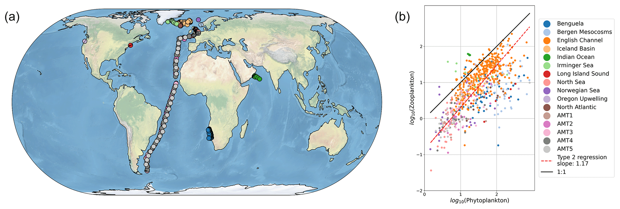
Figure 1 Recent meta-analyses suggest microzooplankton biomass density scales linearly with phytoplankton biomass density in the global ocean. Panel (a) shows the sampling locations, and panel (b) shows the relationship between microzooplankton and phytoplankton biomass in mg C m⁻³ (Rajakaruna et al., 2022; Hatton et al., 2015).

As ecosystem models become increasingly complex, it becomes increasingly challenging to understand how their structure impacts the bulk biogeochemical properties of the system. For example, assumptions about microzooplankton predation on phytoplankton determine model predictions of phytoplankton carbon in the surface ocean, which in turn influences rates of carbon fixation and, eventually, carbon sequestration from the surface layer to the deep ocean. Due to their influence on carbon cycling globally, Earth system models typically contain representations of ocean ecosystems and are incorporating expanded plankton diversity (Séférian et al., 2020), raising questions about how much model complexity is required to capture biogeochemically relevant properties (Kwiatkowski et al., 2014).

Observational datasets provide a critical resource to discriminate between models with different assumptions about modeled food web interactions (Luo et al., 2022; Petrik et al., 2022). The relationship between microbial predators and prey (for example, microzooplankton and phytoplankton, respectively) is one observed phenomenon with profound implications for global biogeochemical cycles, for example by controlling the biomass of autotrophs that fix carbon and impacting carbon export through microzooplankton excretion of fecal pellets (Buck and Newton, 1995). One recent meta-analysis suggests a relatively simple set of observational relationships between microbial predators and their prey (Rajakaruna et al., 2022). Specifically, predator biomass (say, Y) appears to scale with prey biomass (say, X) following a simple linear relationship, i.e., Y∼X (Fig. 1). These observational compilations present the opportunity to identify key features of ocean biogeochemical models that capture relationships between predator and prey biomass.

Here, we undertake this task with a highly idealized set of ecosystem models, solved in the global ocean with a general circulation model. The models we examine are highly abstracted (Fig. 2), capturing some essential features that are general to a wide class of ecosystem and biogeochemical models.

All ecosystem models with descriptions of diversity beyond the classic nutrient–phytoplankton–zooplankton–detritus (NPZD) formulation (Fasham et al., 1990; Wroblewski, 1989) must make assumptions about which predators feed on which prey. However, it is unclear whether empirically rooted contrasting assumptions (Holt et al., 1995; Armstrong, 1999) about predator preference for prey type impact the scaling between predator and prey biomass in a manner that is consistent with patterns observed by Rajakaruna et al. (2022). Our models are put forth specifically to address this question.

In addition to asking whether food web structure impacts plankton predator–prey relationships, we also consider the role of predation in the highest predator, in this case the zooplankton. By their nature, planktonic ecosystem models do not explicitly resolve the dynamics of higher trophic levels. Therefore, the effects of higher predation on the highest predator are usually parameterized (Edwards and Brindley, 1999; Steele and Henderson, 1992; Rhodes and Martin, 2010). The assumptions made here profoundly influence biogeochemical properties such as primary production and chlorophyll distribution (Aumont and Bopp, 2006; Aumont et al., 2015; Stock and Dunne, 2010; Stock et al., 2014; Yool et al., 2013). However, it is unclear if and how their effects are dependent on choices made about food web structure.

By explicitly examining the role of predation in the highest predator in the context of two contrasting food webs, we seek to identify the core, underlying drivers of linear scaling between microbial predators and prey (Fig. 1). We then “sample” the model and compare predictions to observations of trophic structure covering a large range of temperate, subtropical, and tropical ecosystems. In doing so, we evaluate how these contrasting model structures impose trophic structure globally. While our ecosystem models are relatively simple by comparison to many extant biogeochemical models (e.g., Dutkiewicz et al., 2020), they are comparable to the ocean biology component of many extant Earth system models (Rohr et al., 2023) and allow for clear insight. We discuss the implications of our findings for more complex models of ecosystem dynamics.

2 Models and methods

In the sections that follow, we explain and justify the full equations used to parameterize phytoplankton and microzooplankton growth dynamics. We then describe model implementation in a global-ocean ecosystem context and the comparison of simulations with a published compilation of relevant ocean data.

2.1 Food web models

The main ecosystem model parameterization is reported in Box 1, and a schematic representation is provided in Fig. 2. Model equations are described in detail in the Appendix, and our source code is provided in a publicly available repository (https://github.com/werdna-spatial/GUD_closure, last access: 25 March 2024). The most important model parameters are provided in Tables 1 and 2, a more complete list is provided in Table A3, and a fully exhaustive list is provided in the online GitHub repository. We compared predictions of a model with a diamond food web structure (shared predation) to a model assuming predators feed in parallel on distinct prey types in the following sections.

Parallel food chain model. Here it was assumed that microzooplankton grazers feed in parallel on microzooplankton prey (Armstrong, 1999; Ward et al., 2013, 2012), mimicking predation that is specific to different size classes or functional groups. Models with parallel feeding have led to realistic predictions of plankton community composition in the global ocean (Ward et al., 2013; Dutkiewicz et al., 2020). Furthermore, parallel feeding was a component of 5 out of 10 Earth system models that were part of the most recent Coupled Model Intercomparison Project (CMIP6) evaluated by Rohr et al. (2023), making it a useful food web structure to examine in a global-ocean context.

Diamond food web model. An alternative to parallel feeding is a model with shared predation. Here, microzooplankton predators may feed on multiple plankton types. Since this general predation resembles a diamond, models with shared predation are referred to as having a “diamond” food web structure (Holt et al., 1995). A recent study examining plankton community composition along a resource availability gradient in the North Pacific indicated a model with shared predation on Prochlorococcus, and heterotrophic bacteria may, in some circumstances, lead to improved predictions of plankton community composition (Follett et al., 2022). Furthermore, shared predation was a component of 6 out of 10 CMIP6 Earth system models evaluated by Rohr et al. (2023), making it a useful model structure to examine in a global-ocean context.

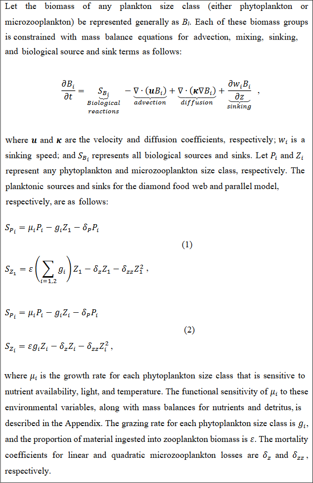
Box 1 Plankton ecosystem model equations.

The parallel food chain and diamond food web models use established allometric scaling laws to assign traits according to phytoplankton cell size (Banse, 1976; Litchman et al., 2007; Ward et al., 2012; see Appendix). In both formulations, small and large phytoplankton represent cells with a ∼0.5 and 5 µm equivalent spherical radius and are representative of picocyanobacteria and eukaryotic algae, respectively. In the parallel model, small and large microzooplankton represent protists with a ∼7 and 50 µm equivalent spherical radius and are representative of microzooplankton in the ciliate size range. The generalist predator in the diamond food web model has a 15 µm equivalent cell radius.

2.2 Parameterizing microzooplankton mortality

All lower trophic ecosystem models must make choices about the mortality of the highest predator. Here, loss processes must be mimicked without being explicitly resolved. This requirement to parameterize presents a problem for plankton ecosystem modelers wishing to motivate model form and function with mechanism. Nevertheless, one way to evaluate the strength of different assumptions about model closure is to examine the influence of contrasting assumptions on the model predictions in a holistic manner. Here, we sought to do this by applying two widely assumed microzooplankton loss processes, as can be seen in the following sections.

Linear microzooplankton losses. Here, it is assumed that the rate of microzooplankton mortality is independent of its biomass density (Box 1). As such, linear losses may equivalently be thought of as density-independent mortality. This assumption has been applied within ecological and biogeochemical models to predict the biogeography of cyanobacteria and heterotrophic bacteria in the North Pacific (Follett et al., 2022) and in the global ocean (Ward et al., 2012, 2013).

Quadratic microzooplankton losses. Here, the rate of microzooplankton mortality increases with biomass density. This increase in the mortality rate can be justified on several grounds, including intraspecific competition (Barbier and Loreau, 2019) and sinking (Schartau et al., 2007), which may both increase with microzooplankton density. Here, we invoke density-dependent mortality on the highest trophic level to mimic the effects of unresolved predation on the highest predator.

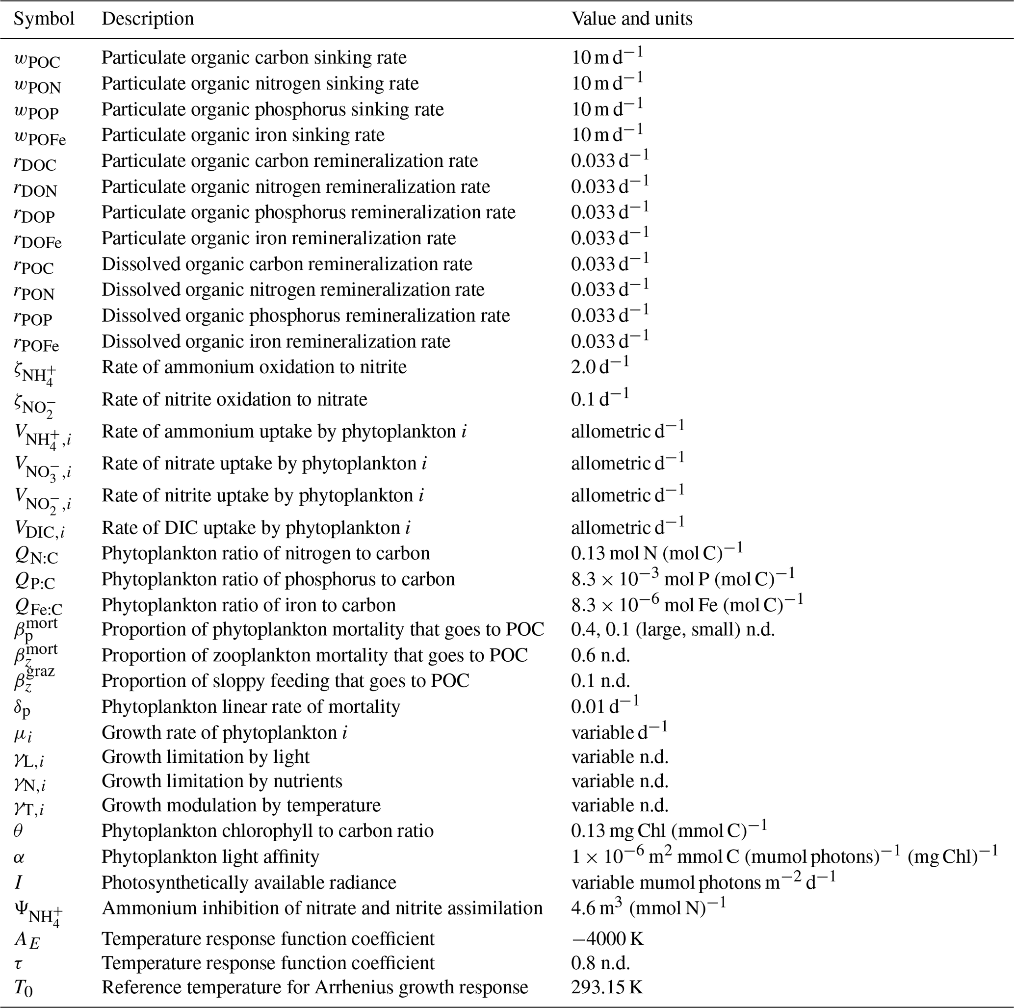
Table 1 Size-independent parameters. All parameters were held constant in all simulations, except for the linear and quadratic mortality terms, which were set to zero in simulations where these terms were not considered. Nondimensional units are represented by n.d.

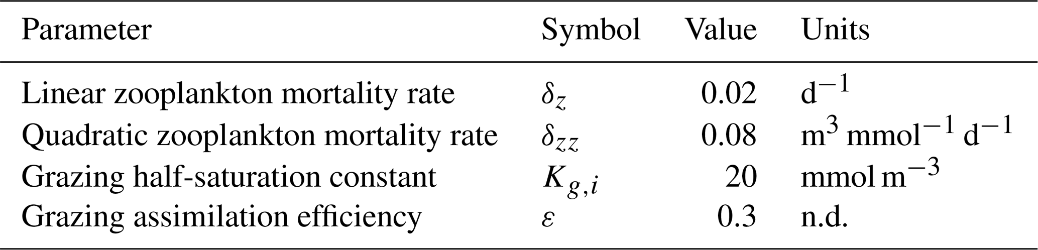
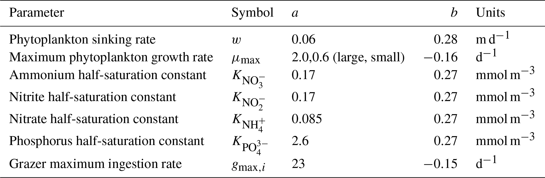
Table 2 Size-dependent parameters and scaling coefficients. Coefficients a and b constrain allometric relations of the form aV^b, where V represents cell volume (µm³). Scaling parameters and coefficients were held constant across all simulations.

2.3 Global-ocean ecosystem models

To explore the ecological and biogeochemical implications of these characteristics, we introduced these parameterizations of primary and secondary producers into a global-ocean ecosystem, biogeochemistry, and circulation model (MITgcm). The ecosystem model simulates flow of C, N, and other elements (Fig. 2) between inorganic nutrients, photo-autotrophs, microzooplankton, and detritus. It is embedded in a coarse-resolution (1°×1° horizontal, 24 vertical levels), climatologically averaged, global-ocean circulation model that has been constrained with satellite and in situ observations (Wunsch and Heimbach, 2007).

2.4 Model data comparison and statistical analyses

We sampled the model in locations where there are environmental samples in the compilation of Rajakaruna et al. (2022) (Fig. 1). After log-transforming phytoplankton and microzooplankton biomass density, we conducted an ordinary least squares type 2 (OLS II) regression and quantified a Pearson correlation coefficient. We compared the regression slope and Pearson R value between the models and the environmental datasets. To identify whether sampling locations were representative of the broader global ecosystem, we repeated the same analysis, sampling the entire global ocean. In doing so, we asked which model assumptions were necessary for the ecosystem model to internally reproduce the observed relationships between microzooplankton and phytoplankton biomass density (Fig. 1).

2.5 Sensitivity studies

Our assumed phytoplankton and zooplankton sizes are narrow by comparison to the diversity of plankton sizes that exists in nature, which in some cases is captured by other ecosystems (Dutkiewicz et al., 2020; Ward et al., 2012) and Earth system models (Kearney et al., 2021). To assess the sensitivity of our findings in relation to assumptions about plankton size, we conducted simulations for all four models in which the (i) phytoplankton volume was increased ∼3-fold, (ii) zooplankton volume was increased ∼3-fold, and (iii) phytoplankton and zooplankton volumes were both increased ∼3-fold.

Predator feeding assumptions profoundly influence modeled dynamics of phytoplankton and microzooplankton (Rohr et al., 2022). To evaluate the sensitivity of our findings to assumptions about plankton feeding, we conducted simulations in which (i) the microzooplankton in the diamond model were allowed to actively switch feeding preference to more abundant prey (see Vallina et al., 2014, and Appendix Eq. A21), and (ii) microzooplankton preyed upon phytoplankton according to a type III feeding curve (see Rohr et al., 2022, and Appendix Eq. A21).

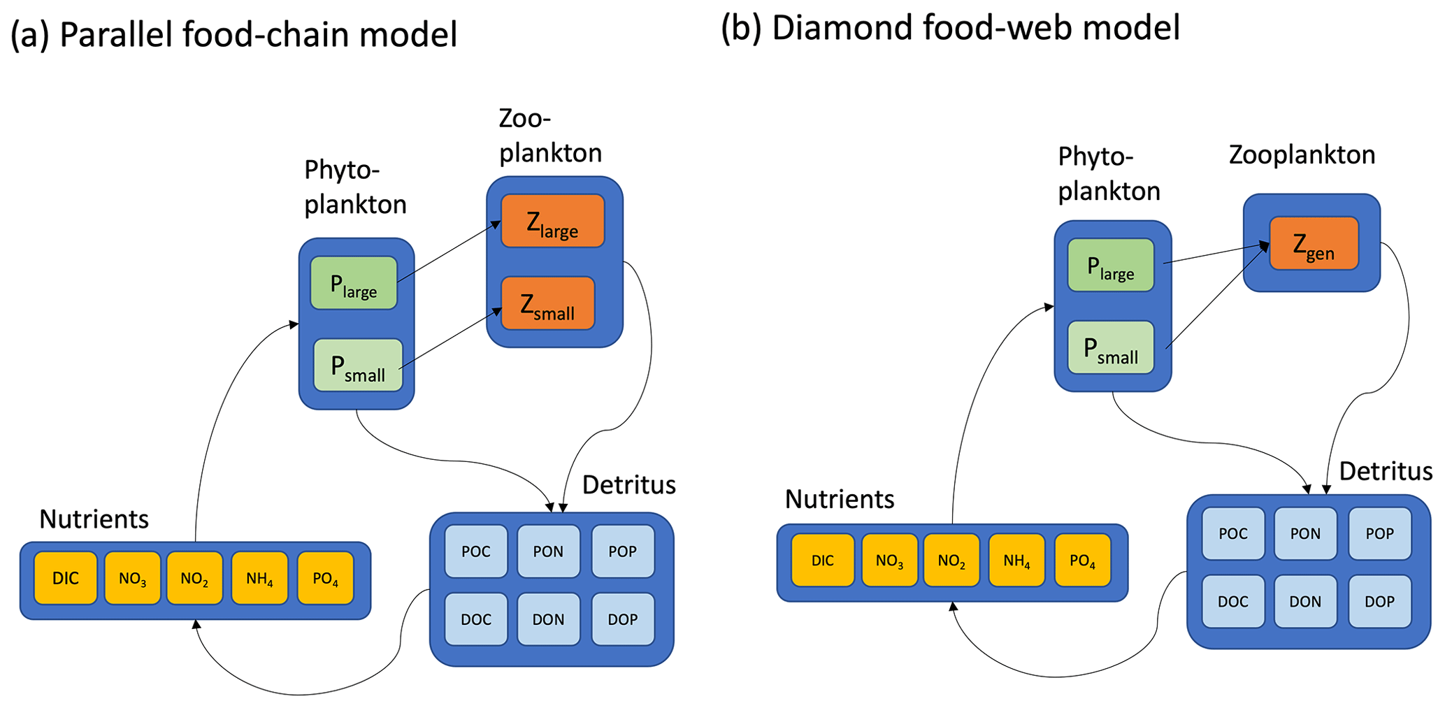
Figure 2 Two contrasting models considered here are (a) the parallel food chains and (b) the shared predation in the form of a diamond food web. Both models cycle elements (C, N, and P) through inorganic and organic forms. Iron biogeochemistry was included in the model in a manner similar to C, N, and P but is not shown for parsimony. Model equations, along with parameter definitions and units, are detailed in the Appendix.

3 Results

We first describe model predictions of ecosystem structure in the global ocean and go on to examine which of the models leads to predictions of predator and prey biomass density, consistent with the observations in Fig. 1. In all that follows, we compare the predictions for both the diamond and parallel food chain models with and without density-dependent microzooplankton losses.

3.1 Surface ocean phytoplankton carbon

All models make qualitatively similar predictions of surface ocean total planktonic carbon (Fig. 3). Plankton carbon density is lowest in the low-latitude oligotrophic gyres and highest in coastal regions, in the equatorial upwelling, and at high latitude. These predictions are all qualitatively consistent with predictions of phytoplankton biomass density indicated by satellite remote sensing of ocean color (Hu et al., 2019). Interestingly, however, there are clear differences in the total plankton carbon density predicted by the four models, with the most notable contrast between the models with parallel feeding and the diamond food web (compare columns in Fig. 3). Specifically, the model with parallel feeding tends to predict a greater total phytoplankton carbon density at high latitude and in equatorial upwelling and coastal regions. There are more subtle increases in total plankton carbon density when quadratic microzooplankton losses are assumed instead of linear microzooplankton mortality (compare bottom and top rows in Fig. 3). The quadratic closure allows for a far greater contribution of phytoplankton to total carbon (Figs. S1 and S2 in the Supplement), raising total planktonic carbon inventories globally (Fig. 3). Qualitatively similar differences in these four models are found in depth-integrated primary production (Fig. S3), carbon export (Fig. S4), and secondary production (Fig. S5). These results identify a subtle interplay between food web structure and microzooplankton mortality in predictions of plankton carbon density in the global ocean.

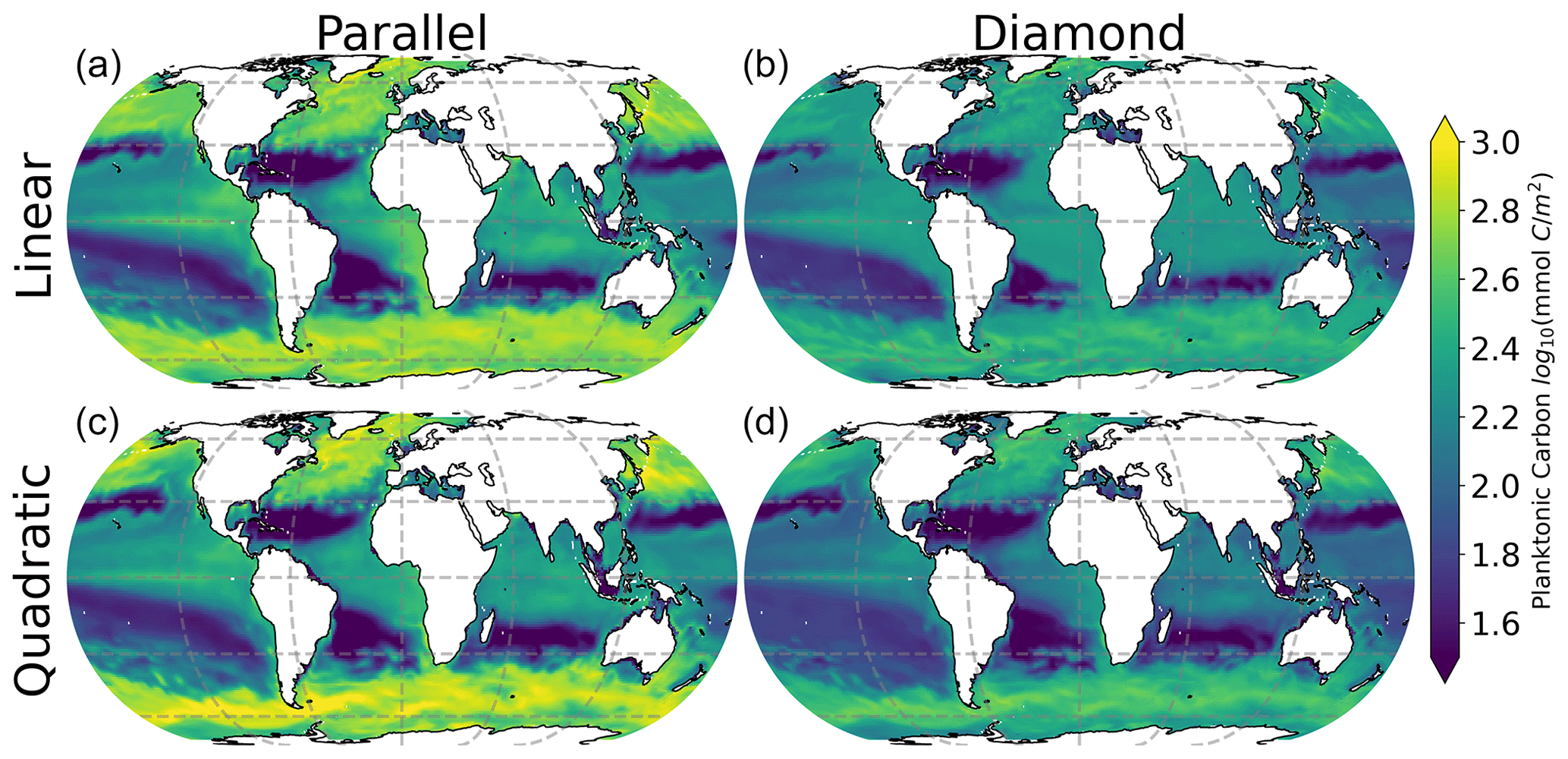
Figure 3 Depth-integrated total plankton carbon predicted by all four contrasting models. Color represents total plankton carbon density averaged over a seasonal cycle.

3.2 Surface ocean community composition

All four models predict qualitatively similar patterns in phytoplankton community composition in the surface ocean (Fig. 4). Specifically, the small phytoplankton size class dominates in the low-latitude oligotrophic gyres (deep red colors in Fig. 4), and the large phytoplankton size class dominates at high latitudes (deep blue colors in Fig. 4). Nevertheless, the model with shared predation (diamond food web) predicts far greater competitive exclusion of the small phytoplankton size class at high latitude. The parallel food web model predicts coexistence of the small and large phytoplankton throughout much of the surface ocean, regardless of which microzooplankton closure is used (left-hand column in Fig. 4).

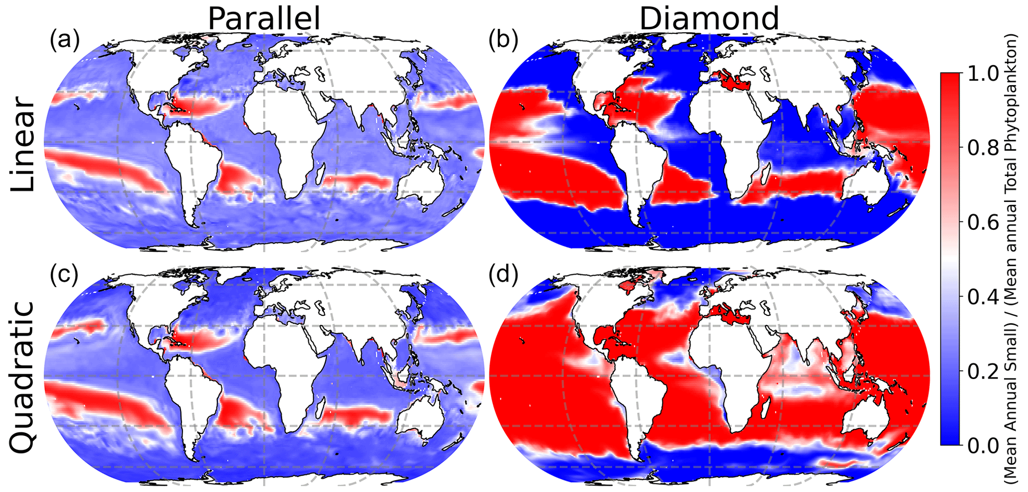
Figure 4 Phytoplankton community composition in the surface ocean. Red indicates dominance of small phytoplankton; blue indicates dominance of large phytoplankton.

3.3 Interplay between community composition and total carbon density

Interestingly, the impact of food web structure (diamond vs. parallel) and microzooplankton closure (linear vs. quadratic) appears to be mirrored in the model predictions of plankton carbon density (Fig. 3) and community composition (Fig. 4). Specifically, the greatest differences are between the diamond and parallel models (comparing columns), with more nuanced differences between closure assumption (comparing rows). This mirroring points to community composition as a driver of total plankton carbon density. Specifically, anywhere in the ocean with greater representation of the smaller size class tends to predict an elevated total plankton carbon density.

3.4 Quadratic microzooplankton closure predicts global trophic structure

The results in Figs. 3–4 point to the importance of a food web structure for predictions of planktonic ecosystem carbon in the global ocean. We now turn our attention to ask the following question: which of these models is consistent with observations that microzooplankton carbon density scales linearly with phytoplankton carbon density (Fig. 1, Rajakaruna et al., 2022)?

In Fig. 5, we show the relationship between total microzooplankton and phytoplankton carbon for the global ocean. Each colored point represents the number of 1° grid cells falling within the microzooplankton and phytoplankton carbon density marked by its position on the axes. The dashed black line represents the OLS II regression slope. Interestingly, we find here that any differences between the parallel and diamond food web are minimal (compare columns, Fig. 5), and the largest differences are between the linear and quadratic microzooplankton closure (compare rows, Fig. 5). Therefore, in predicting ecosystem trophic structure, which we think of here as the relationship between microzooplankton and phytoplankton carbon density, the impacts of food web on phytoplankton community composition that were revealed in Figs. 3–4 cease to play an important role. Moreover, only the model with quadratic microzooplankton losses predicts a relationship between microzooplankton and phytoplankton carbon density that is consistent with the linear scaling in the observation dataset in Fig. 1 (bottom row of Fig. 5). The model with linear microzooplankton mortality predicts far less correlation between microzooplankton and phytoplankton carbon density (reflected in the lower r values) and a negative slope that relates total microzooplankton carbon with phytoplankton carbon.

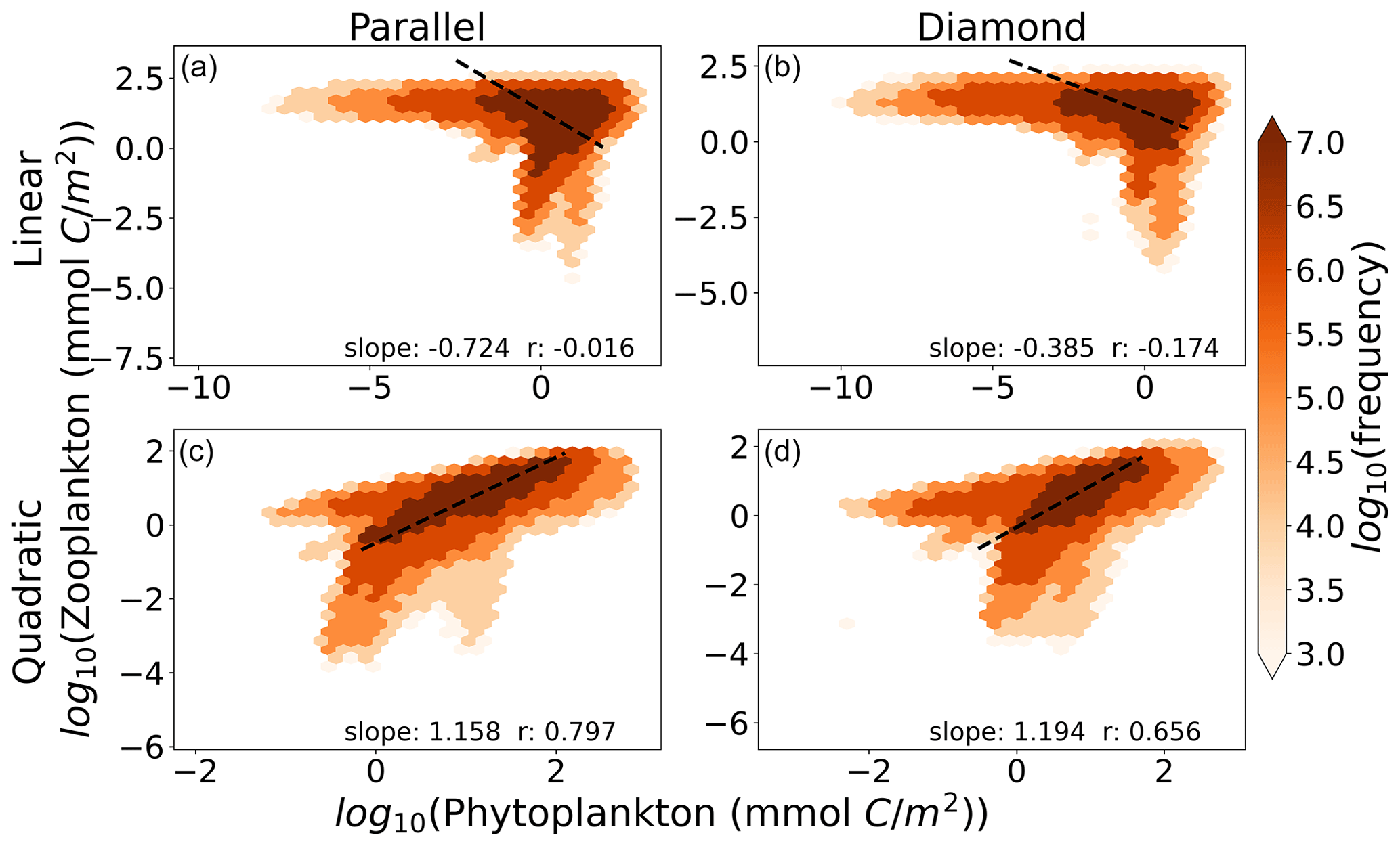
Figure 5 The relationship between phytoplankton and microzooplankton carbon density in the global ocean for the (a) parallel food chain model with linear closure, (b) diamond food web with linear closure, (c) parallel food chain model with quadratic closure, and (d) diamond food web model with quadratic closure. The color within each hexagon represents the number of 1° grid cells that fall within the biomass range marked by their position on the axes. Slopes are OLS type II regression slopes, and r values are Pearson correlation coefficients. Density-dependent microzooplankton mortality reproduces the relationship between Z and P, regardless of food web structure.

Why does the linear closure predict such a variable relationship between microzooplankton and phytoplankton carbon density? To investigate these predictions, we attempted to separate out spatial and temporal impacts on the relationship.

In Fig. 6, we show seasonal variability in the relationship between microzooplankton and phytoplankton carbon density for a single site in the English Channel. Observations of time-dependent biomass dynamics (Fig. 6a) are associated with a strikingly linear relationship between microzooplankton and phytoplankton biomass density (Fig. 6b). Consistent with prior analyses (Steele and Henderson, 1992; Fasham, 1995; Edwards and Brindley, 1999; Edwards and Yool, 2000), models with linear zooplankton losses predict oscillations in phytoplankton and microzooplankton biomass (Fig. 6c, e), irrespective of whether a parallel or diamond food web structure is assumed. The regression slopes for this single location mirror the regression slopes for the global ocean; the linear microzooplankton closure predicts a shallow regression slope with low r value (Fig. 6d, f), and the quadratic closure predicts a far higher correlation between phytoplankton and microzooplankton biomass (Fig. 6h, j), again consistent with the global collection (Fig. 5). Notably, there are many inconsistencies between the modeled time-dependent biomass dynamics and the observations (Fig. 6). For example, the quadratic closure predicts a premature spring bloom initiation and termination (Fig. 6g, i). Therefore, the correct relationship between phytoplankton and microzooplankton biomass density can be retrieved even when the bloom dynamics are incorrect, pointing to the limitation of biomass-scaling relationships as a sole indicator of model performance. Nevertheless, these results demonstrate the tendency of the linear closure to predict predator–prey oscillations as a key driver of the global relationship between phytoplankton and microzooplankton biomass density. The cyclic behavior is true, irrespective of assumptions about parallel food chains vs. a diamond food web.

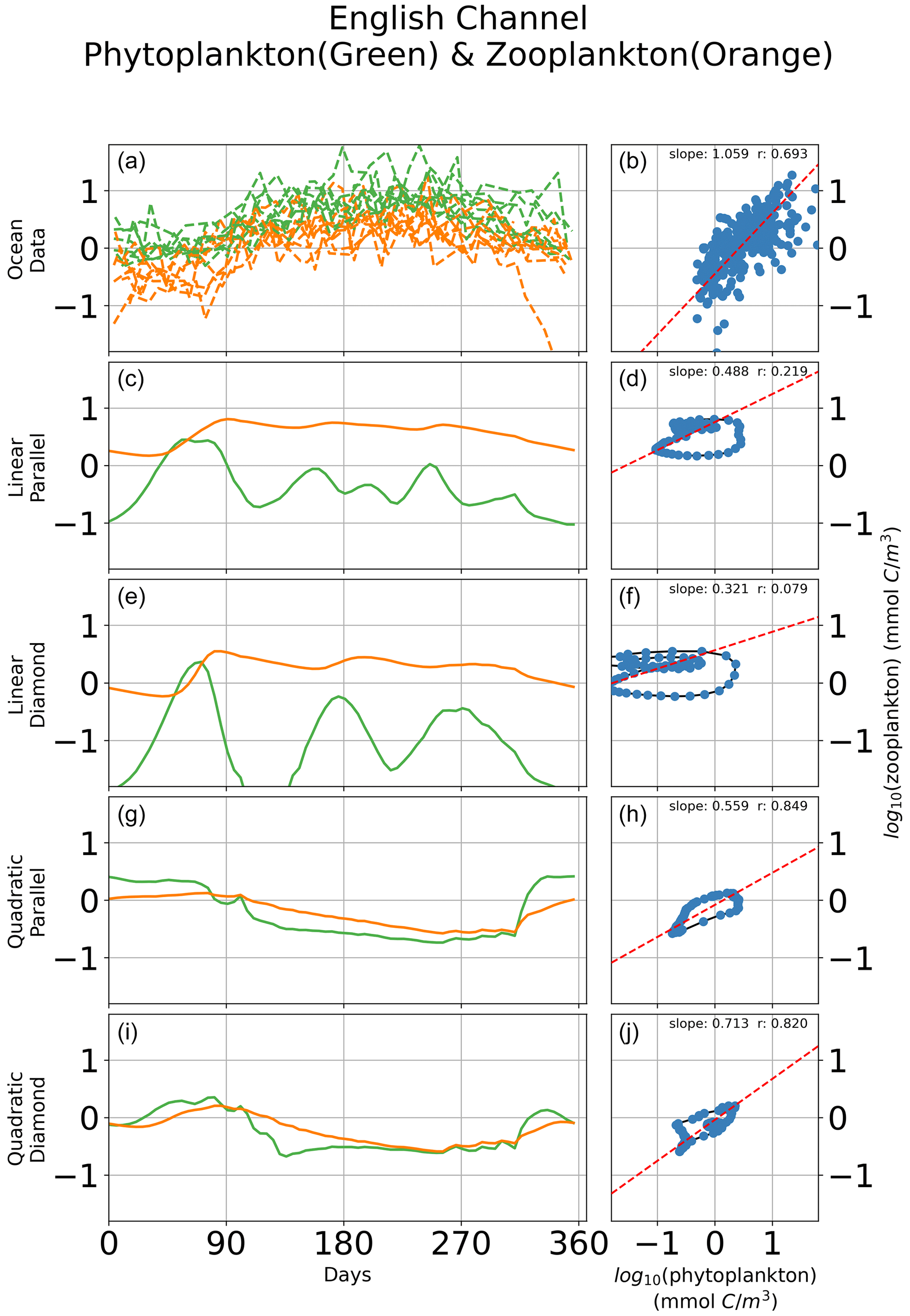
Figure 6 Time-dependent biomass dynamics in observational data (a) and across models (c, e, g, i) with corresponding relationships between total microzooplankton and phytoplankton carbon density (b, d, f, h, j) during a seasonal cycle in the English Channel. Linear losses of the microzooplankton predict cyclic behavior in the predator–prey relationship that are inconsistent with observations (Fig. 1).

In Fig. 7, we show spatial variation in the Z:P biomass ratio in the surface ocean, where the color in each location represents the seasonally averaged Z:P biomass ratio. Interestingly, there is considerable spatial variability in Z:P for either food web assuming a linear closure (top row of Fig. 7), with the Z:P biomass ratio rising at higher latitudes (top row of Fig. 7). This prediction is consistent with prior estimates of Z:P biomass variability in the global ocean that assumed linear closure and parallel feeding (Ward et al., 2012). The quadratic closure removes much of this spatial variation (note the narrower color bar range in the bottom row of Fig. 7). In a steady state, linear losses on the microzooplankton allow them to place a limit on the phytoplankton biomass, causing carbon to accumulate in the predator (Follett et al., 2022). Density-dependent mortality on the microzooplankton forces the microzooplankton to be removed at a rate that is commensurate with their biomass density, inhibiting their ability to limit the phytoplankton population size and causing both predators and prey to rise together as the system is enriched with resources.

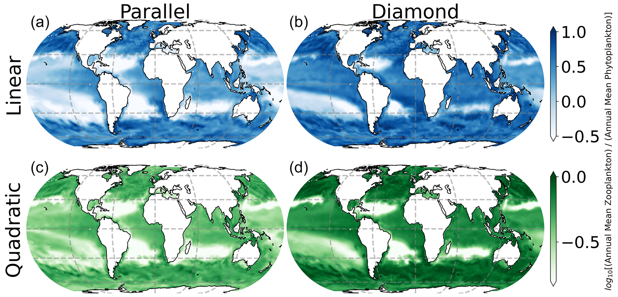
Figure 7 Seasonally averaged surface ocean Z:P biomass ratio. Spatial variability in the Z:P ratio is lessened by quadratic microzooplankton losses, irrespective of food web structure.

Our findings regarding quadratic closure as a driver of linear phytoplankton and microzooplankton biomass scaling are insensitive to different assumptions about phytoplankton and microzooplankton size (Fig. S6). Furthermore, allowing microzooplankton to actively switch to prey on more-abundant phytoplankton allows for a greater coexistence of phytoplankton in the diamond food web (Fig. S7; Vallina et al., 2014) but unsurprisingly does not qualitatively modify the scaling relationships reported in Fig. 5. Microzooplankton feeding according to type III functional response leads to a far greater correlation between predators and prey across models (Fig. S8). These results are consistent with prior studies identifying type III feeding as a stabilizing mechanism on microzooplankton–phytoplankton dynamics (Rohr et al., 2022). Nevertheless, even when a type III response is assumed, the quadratic closure still leads to a more realistic correlation between microzooplankton and phytoplankton than the linear closure (Fig. S8), pointing to the quadratic closure as an important control on trophic structure globally.

4 Discussion

Microzooplankton predation on phytoplankton determines phytoplankton carbon in the surface ocean, which in turn influences rates of carbon fixation and, eventually, carbon sequestration from the surface layer to the deep ocean. Models of plankton ecosystem structure are becoming increasingly complex, but models with relatively simple representation of plankton food webs are important components of many extant Earth system models (Rohr et al., 2023). Here, we have examined a set of models with minimal complexity, in the context of environmental data, to examine core drivers of a system structure globally. We find that the total phytoplankton carbon density, and community composition, is profoundly impacted by choices regarding food web structure and losses on the highest predator (in this case, microzooplankton grazers). The diamond food web predicts competitive exclusion of small and large phytoplankton size classes, whereas parallel feeding allows the small phytoplankton size class to persist throughout much of the surface ocean during high latitude blooms and in coastal upwelling regions.

The persistence of small phytoplankton size classes at higher latitudes is consistent with observational data showing that picoplankton (<2 µm) and nanoplankton (2–20 µm) persist through temperature and resource gradients in a wide range of ocean environments (Marañón et al., 2012). These findings, in tandem with our study and prior modeling studies (Ward et al., 2012, 2013), point to parallel feeding as a pervasive influence on planktonic system structure. Nevertheless, shared predation has been invoked to explain Prochlorococcus die-off with latitude (Follett et al., 2022) and is invoked in many extant Earth system models (Rohr et al., 2023). Therefore, both food web structures considered here (parallel feeding and the diamond food web) may exist in natural planktonic systems and are also assumed within models of the global ocean that inform climate change projections. Our findings point to the need to carefully consider assumptions about predation on the highest trophic level with application of either model structure, since these have profound implications both for phytoplankton carbon inventories and community composition.

The food web model structures assumed here are so simple that they exclude many mechanisms already considered in extant Earth system models. For example, many Earth system models contain representations of both microzooplankton and mesozooplankton. In some cases, these are explicitly represented with multiple state variables (Stock et al., 2014; Aumont et al., 2015). In others, a single “adaptive” zooplankton class mimics the effects of micro- and mesozooplankton by feeding differently on phytoplankton prey types (Moore et al., 2004; Long et al., 2021). Future studies may evaluate the impact of different closures in the context of these more sophisticated structures. Despite the simplicity of our models, we anticipate that our central conclusions will hold in a more general setting. Specifically, assumptions made about highest-predator mortality constrain biomass-scaling relationships regardless of model predictions about community composition within a trophic level.

By comparison to the models considered here, plankton communities are considerably more complex and diverse, regarding organism size (Hansen et al., 1994), metabolism (Alexander et al., 2015; Posfai et al., 2017), and resource affinities (Litchman et al., 2007). Similarly, when it comes to parameterizing microzooplankton losses, there are more complex assumptions to be made beyond our very crude contrast between linear (density-independent) and quadratic (density-dependent) mortality, again with implications for system properties (Omta et al., 2023; Rhodes and Martin, 2010). Despite these limitations, our modeling points to a simple set of principles that we anticipate will extend to more sophisticated representations of plankton ecology. In particular, the quadratic microzooplankton closure provides a realistic and important constraint on the relationship between microzooplankton and phytoplankton carbon density, irrespective of the assumed food web. This generality and consistency with observational data may also apply to other predator–prey interactions. Linear scaling between predator and prey abundance has also been observed between viruses and heterotrophic bacteria (Rajakaruna et al., 2022). Viral infection is thought to be highly host-specific (Flores et al., 2011), suggesting a parallel food web structure between predators and prey may be more appropriate. Our finding that linear scaling between predators and prey can be reproduced with the quadratic closure, regardless of food web structure, provides insight that may inform models of plankton ecosystems that include even more diverse representations of microbial life.

Appendix A: Model description

Here we provide details of the ecosystem model represented graphically in Fig. 2. The description is very similar to other implementations of the Darwin ecosystem model (Ward et al., 2012; Dutkiewicz et al., 2009, 2012; Zakem et al., 2018). All model parameter variable definitions and units are provided in Tables 1 and 2 of the main text and Tables A1–A3 of this appendix. An exhaustive list of all parameter values can be found in the online code repository (https://github.com/werdna-spatial/GUD_closure, last access: 25 March 2024).

Dissolved organic and inorganic material are all governed by a mass balance for advection, diffusion, and biological sources and sinks:

$$\begin{array}{}\text{(A1)}& {\displaystyle \frac{\partial X}{\partial t}}=\underset{\text{biological reactions}}{\underbrace{S_X}}-\underset{\text{advection}}{\underbrace{\mathrm{\nabla }\cdot \left(\mathit{u}X\right)}}+\underset{\text{diffusion}}{\underbrace{\mathrm{\nabla }\cdot \left(\mathit{\kappa }\mathrm{\nabla }X\right)}},\end{array}$$

where X represents ammonium, nitrate, nitrite, phosphorus, dissolved inorganic carbon (DIC), and iron, as well as pools of dissolved organic carbon, nitrogen, phosphorus, and iron. Pools of particulate detritus follow a similar mass balance but are also assumed to sink at rate w_Y:

$$\begin{array}{}\text{(A2)}& {\displaystyle \frac{\partial Y}{\partial t}}=S_Y-\mathrm{\nabla }\cdot \left(\mathit{u}Y\right)+\mathrm{\nabla }\cdot \left(\mathit{\kappa }Y\right)-{\displaystyle \frac{\partial w_{Y}Y}{\partial z}},\end{array}$$

where Y represents carbon, nitrogen, phosphorus, and iron, respectively.

Several of the biological source and sink terms are described in the main text (Box 1). Here, we describe additional source and sink terms for inorganic nutrients and detritus. Ammonium is produced by the remineralization of organic material and lost by nitrification and phytoplankton growth:

$$\begin{array}{}\text{(A3)}& \begin{array}{rl}{S}_{{\mathrm{NH}}_{\mathrm{4}}^{+}}& =\underset{\text{remineralization}}{\underbrace{r_{\text{DON}}\text{DON}+r_{\mathrm{PON}}\text{PON}}}-\underset{\text{nitrification}}{\underbrace{{\mathit{\zeta }}_{{\mathrm{NH}}_{\mathrm{4}}^{+}}{\mathrm{NH}}_{\mathrm{4}}^{+}}}\\ & -\underset{\text{nutrient uptake}}{\underbrace{\sum _j{V}_{{\mathrm{NH}}_{\mathrm{4}}^{+}}{P}_j}}.\end{array}\end{array}$$

Biological source and sink terms for nitrate, nitrite, phosphorus, and dissolved inorganic carbon are as follows:

$$\begin{array}{}\text{(A4)}& {\displaystyle }{S}_{{\mathrm{NO}}_{\mathrm{3}}^{-}}=\underset{\text{nitrification}}{\underbrace{{\mathit{\zeta }}_{{\mathrm{NO}}_{\mathrm{2}}^{-}}{\mathrm{NO}}_{\mathrm{2}}^{-}}}-\underset{\text{nitrate uptake}}{\underbrace{Q_{\mathrm{N}:\mathrm{C}}\sum _j{V}_{{\mathrm{NO}}_{\mathrm{3}}^{-},j}{P}_j}},\text{(A5)}& {\displaystyle }{S}_{{\mathrm{NO}}_{\mathrm{2}}^{-}}=\underset{\text{nitrification}}{\underbrace{{\mathit{\zeta }}_{{\mathrm{NH}}_{\mathrm{4}}^{+}}{\mathrm{NH}}_{\mathrm{4}}^{+}}}-\underset{\text{nitrification}}{\underbrace{{\mathit{\zeta }}_{{\mathrm{NO}}_{\mathrm{2}}^{-}}{\mathrm{NO}}_{\mathrm{2}}^{-}}}-\underset{\text{nitrate uptake}}{\underbrace{Q_{\mathrm{N}:\mathrm{C}}\sum _j{V}_{{\mathrm{NO}}_{\mathrm{2}}^{-},j}{P}_j}},\text{(A6)}& {\displaystyle }{S}_{{\mathrm{PO}}_{\mathrm{4}}^{\mathrm{3}-}}=\underset{\text{remineralization}}{\underbrace{r_{\mathrm{DOP}}\mathrm{DOP}+r_{\mathrm{POP}}\mathrm{POP}}}-\underset{\text{phosphate uptake}}{\underbrace{Q_{\mathrm{P}:\mathrm{C}}\sum _j{V}_{\mathrm{DIC},j}{P}_j}},\text{(A7)}& {\displaystyle }{S}_{\mathrm{DIC}}=\underset{\text{remineralization}}{\underbrace{r_{\mathrm{DOC}}\mathrm{DOC}+r_{\mathrm{POC}}\mathrm{POC}}}-\underset{\text{DIC uptake}}{\underbrace{\sum _j{V}_{\mathrm{DIC},j}{P}_j}},\text{(A8)}& {\displaystyle }{S}_{\mathrm{Fe}}=\underset{\text{remineralization}}{\underbrace{r_{\mathrm{DOFe}}\mathrm{DOFe}+r_{\mathrm{POFe}}\mathrm{POFe}}}-\underset{\text{iron uptake}}{\underbrace{Q_{\mathrm{Fe}:\mathrm{C}}\sum _j{V}_{\mathrm{DIC},j}{P}_j}},\end{array}$$

where fixed elemental ratios convert carbon uptake to other elements (e.g., multiplication by Q_P:C in Eq. A6 converts carbon uptake to phosphorus uptake).

Dissolved organic material, for example DOC, is produced through phytoplankton and zooplankton mortality and sloppy feeding and consumed through remineralization:

$$\begin{array}{}\text{(A9)}& \begin{array}{rl}& S_{\mathrm{DOC}}=\underset{\text{phytoplankton mortality}}{\underbrace{\sum _i(\mathrm{1}-{\mathit{\beta }}_p^{\mathrm{mort}}){\mathit{\delta }}_p{P}_i}}+\underset{\text{zooplankton mortality}}{\underbrace{\sum _j(\mathrm{1}-{\mathit{\beta }}_z^{\mathrm{mort}})({\mathit{\delta }}_z{Z}_j+{\mathit{\delta }}_{zz}{Z}_j^{\mathrm{2}})}}\\ & +\underset{\text{sloppy feeding}}{\underbrace{\sum _i\sum _j(\mathrm{1}-{\mathit{\beta }}_z^{\mathrm{graz}})(\mathrm{1}-\mathit{\epsilon })g_i{Z}_j}}-\underset{\text{remineralization}}{\underbrace{r_{\mathrm{DOC}}\mathrm{DOC}}}.\end{array}\end{array}$$

Dissolved nitrogen and phosphorus are governed by the same sources and sinks and converted from carbon with fixed stoichiometric ratios, e.g., for nitrogen Q_N:C (units mol N (mol C)⁻¹):

$$\begin{array}{}\text{(A10)}& \begin{array}{rl}{S}_{\mathrm{DON}}& =\underset{\text{phytoplankton mortality}}{\underbrace{Q_{\mathrm{N}:\mathrm{C}}\sum _i(\mathrm{1}-{\mathit{\beta }}_p^{\mathrm{mort}}){\mathit{\delta }}_p{P}_i}}\\ & +\underset{\text{zooplankton mortality}}{\underbrace{Q_{\mathrm{N}:\mathrm{C}}\sum _j(\mathrm{1}-{\mathit{\beta }}_z^{\mathrm{mort}})({\mathit{\delta }}_z{Z}_j+{\mathit{\delta }}_{\mathrm{zz}}{Z}_j^{\mathrm{2}})}}\\ & +\underset{\text{sloppy feeding}}{\underbrace{Q_{\mathrm{N}:\mathrm{C}}\sum _i\sum _j(\mathrm{1}-{\mathit{\beta }}_z^{\mathrm{graz}})(\mathrm{1}-\mathit{\epsilon })g_i{Z}_j}}\\ & -\underset{\text{remineralization}}{\underbrace{r_{\mathrm{DON}}\mathrm{DON}}}.\end{array}\end{array}$$

The same basic processes are also biological sources and sinks for particulate organic carbon:

$$\begin{array}{}\text{(A11)}& \begin{array}{rl}{S}_{\mathrm{POC}}=& \underset{\text{phytoplankton mortality}}{\underbrace{\sum _i{\mathit{\beta }}_p^{\mathrm{mort}}{\mathit{\delta }}_p{P}_i}}\\ & +\underset{\text{zooplankton mortality}}{\underbrace{\sum _j{\mathit{\beta }}_z^{\mathrm{mort}}({\mathit{\delta }}_z{Z}_j+{\mathit{\delta }}_{zz}{Z}_j^{\mathrm{2}})}}\\ & +\underset{\text{sloppy feeding}}{\underbrace{\sum _i\sum _j{\mathit{\beta }}_z^{\mathrm{graz}}(\mathrm{1}-\mathit{\epsilon })g_i{Z}_j}}-\underset{\text{remineralization}}{\underbrace{r_{\mathrm{POC}}\mathrm{POC}}},\end{array}\end{array}$$

where ${\mathit{\beta }}_p^{\mathrm{mort}}$ and ${\mathit{\beta }}_Z^{\mathrm{mort}}$ are given as partitions for phytoplankton and zooplankton losses between particulate and dissolved pools, with corresponding partitions for sloppy feeding given by ${\mathit{\beta }}_p^{\mathrm{graz}}$ and ${\mathit{\beta }}_Z^{\mathrm{graz}}$. As with DOM (Eq. A10), fixed stoichiometric conversations are applied to convert carbon POC sources to PON and POP. These equations are not shown for brevity.

The phytoplankton growth rate μ_i is modified by light, nutrients, and temperature in a multiplicative manner:

$$\begin{array}{}\text{(A12)}& {\mathit{\mu }}_i={\mathit{\mu }}_{\max ,i}{\mathit{\gamma }}_{L,i}{\mathit{\gamma }}_{\mathrm{N},i}{\mathit{\gamma }}_{\mathrm{T},i},\end{array}$$

where light limitation is based on the model of photoacclimation following Geider et al. (1997). This can be seen as follows:

$$\begin{array}{}\text{(A13)}& {\mathit{\gamma }}_{L,i}=\left(\mathrm{1}-\exp \left({\displaystyle \frac{-\mathit{\alpha }\mathit{\theta }I}{{\mathit{\mu }}_{\max ,i}{\mathit{\gamma }}_{\mathrm{N},i}{\mathit{\gamma }}_{\mathrm{T},i}}}\right)\right).\end{array}$$

Nutrient limitation follows Monod kinetics and Liebig's law of the minimum:

$$\begin{array}{}\text{(A14)}& {\mathit{\gamma }}_N=min\left\{V_{\mathrm{N},i},V_{\mathrm{P},i},V_{\mathrm{Fe},i}\right\},\end{array}$$

where nutrient limitation by nitrogen, phosphorus, and iron is governed by Monod kinetics. This can been seen as follows:

$$\begin{array}{}\text{(A15)}& {\displaystyle }\begin{array}{rl}{V}_{\mathrm{N},i}& ={\displaystyle \frac{{\mathrm{NO}}_{\mathrm{3}}^{-}}{{\mathrm{NO}}_{\mathrm{3}}^{-}+K_{{\mathrm{NO}}_{\mathrm{3}}^{-}}}}{e}^{\mathrm{\Psi }{\mathrm{NH}}_{\mathrm{4}}^{+}}+{\displaystyle \frac{{\mathrm{NO}}_{\mathrm{2}}^{-}}{{\mathrm{NO}}_{\mathrm{2}}^{-}+K_{{\mathrm{NO}}_{\mathrm{2}}^{-}}}}\\ & e^{\mathrm{\Psi }{\mathrm{NH}}_{\mathrm{4}}^{+}}+{\displaystyle \frac{{\mathrm{NH}}_{\mathrm{4}}^{+}}{{\mathrm{NH}}_{\mathrm{4}}^{+}+K_{{\mathrm{NH}}_{\mathrm{4}}^{+}}}},\end{array}\text{(A16)}& {\displaystyle }{V}_{\mathrm{P},i}={\displaystyle \frac{{\mathrm{PO}}_{\mathrm{4}}^{\mathrm{3}-}}{{\mathrm{PO}}_{\mathrm{4}}^{\mathrm{3}-}+K_{{\mathrm{PO}}_{\mathrm{4}}^{\mathrm{3}-}}}},\text{(A17)}& {\displaystyle }{V}_{\mathrm{Fe},i}={\displaystyle \frac{\mathrm{Fe}}{\mathrm{Fe}+K_{\mathrm{Fe}}}},\end{array}$$

where nitrate and nitrite assimilation are inhibited in the presence of ammonium with Ψ, following Follows et al. (2007) and others (Ward et al., 2012; Dutkiewicz et al., 2009, 2012; Zakem et al., 2018). Uptakes of ammonium, nitrite, and nitrate are found by partitioning total realized nutrient uptake by the three different nitrogen species as follows:

$$\begin{array}{}\text{(A18)}& {\displaystyle }{V}_{{\mathrm{NH}}_{\mathrm{4}}^{+},i}={\displaystyle \frac{\mathrm{1}}{V_{\mathrm{N},i}}}{\displaystyle \frac{{\mathrm{NH}}_{\mathrm{4}}^{+}}{{\mathrm{NH}}_{\mathrm{4}}^{+}+K_{{\mathrm{NH}}_{\mathrm{4}}^{+}}}}{\mathit{\gamma }}_N,\text{(A19)}& {\displaystyle }{V}_{{\mathrm{NO}}_{\mathrm{2}}^{-},i}={\displaystyle \frac{\mathrm{1}}{V_{\mathrm{N},i}}}{\displaystyle \frac{{\mathrm{NO}}_{\mathrm{2}}^{-}}{{\mathrm{NO}}_{\mathrm{2}}^{-}+K_{{\mathrm{NO}}_{\mathrm{2}}^{-}}}}{e}^{\mathrm{\Psi }{\mathrm{NH}}_{\mathrm{4}}^{+}}{\mathit{\gamma }}_N,\text{(A20)}& {\displaystyle }{V}_{{\mathrm{NO}}_{\mathrm{3}}^{-},i}={\displaystyle \frac{\mathrm{1}}{V_{\mathrm{N},i}}}{\displaystyle \frac{{\mathrm{NO}}_{\mathrm{3}}^{-}}{{\mathrm{NO}}_{\mathrm{3}}^{-}+K_{{\mathrm{NO}}_{\mathrm{3}}^{-}}}}{e}^{\mathrm{\Psi }{\mathrm{NH}}_{\mathrm{4}}^{+}}{\mathit{\gamma }}_N.\end{array}$$

Growth is modulated by temperature with the Arrhenius equation:

$$\begin{array}{}\text{(A21)}& {\mathit{\gamma }}_T=\mathit{\tau }\exp \left(A_E\left({\displaystyle \frac{\mathrm{1}}{T+\mathrm{273.15}}}-{\displaystyle \frac{\mathrm{1}}{T_{\mathrm{0}}}}\right)\right).\end{array}$$

The grazing rate of zooplankton type j follows a type II or III functional response as a function of total phytoplankton biomass (Holling, 1959), partitioned between phytoplankton size classes according to the proportion of total phytoplankton biomass in each size class:

$$\begin{array}{}\text{(A22)}& g_{i,j}=g_{\max ,j}{\displaystyle \frac{P_i^{\mathit{\beta }}}{\sum _i{P}_i^{\mathit{\beta }}}}{\displaystyle \frac{(\sum _i{P}_i{)}^{\mathit{\gamma }}}{(\sum _i{P}_i{)}^{\mathit{\gamma }}+K_{g,j}^{\mathit{\gamma }}}},\end{array}$$

where the value of β switches the grazers from passive (β=1) to active (β=2) switching and the value of γ switches from a type II (γ=2) to a type III (γ=3) functional response (Vallina et al., 2014). Our main simulations assumed passive switching and type II functional response, but we conducted sensitivities to both assumptions, separately allowing active-prey switching and type III functional response.

Table A1 Model state variables.

Table A2 Biological source and sink variables.

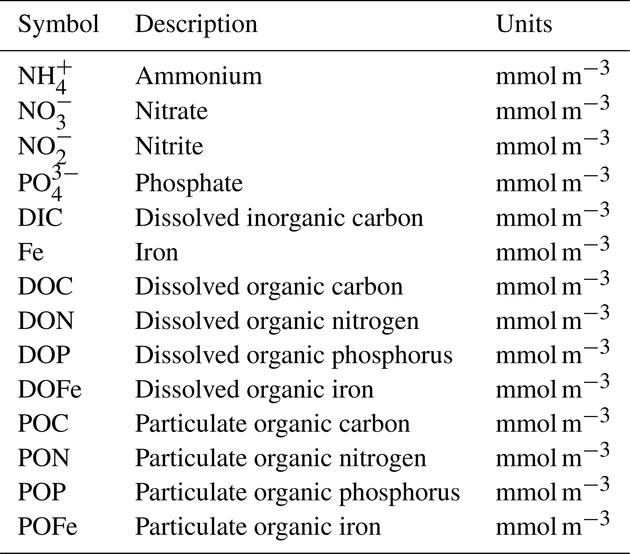
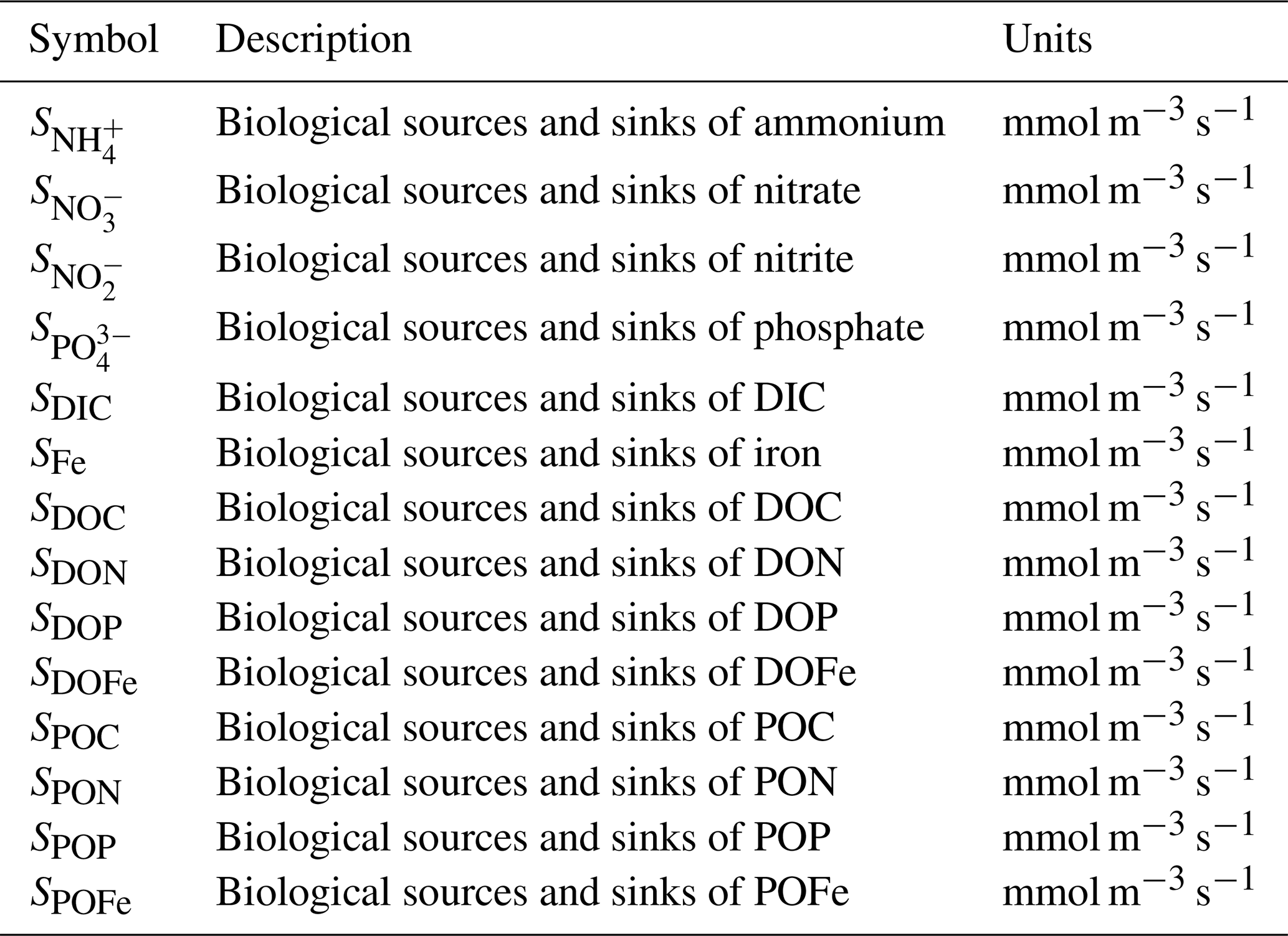
Table A3 Model parameters and variables. Specific parameter values assume default values listed in various publications (Ward et al., 2012; Dutkiewicz et al., 2020) and are available in our online repository (https://github.com/werdna-spatial/GUD_closure/tree/main/Paper_Data, last access: 25 March 2024). Plankton traits (nutrient and grazing half-saturation constants, maximal grazing, and nutrient uptake rates) were generated via allometric scaling relationships reported by Ward et al. (2012), and a subset of these is reported in Table 3. The large phytoplankton has a faster maximal growth rate and higher nutrient half-saturation constants than the small phytoplankton, representative of differences in growth rate between a eukaryotic algae and a cyanobacteria, respectively (Tables 2 and 3; Litchman et al., 2007; Ward et al., 2012).