the Creative Commons Attribution 4.0 License.
the Creative Commons Attribution 4.0 License.
 | 05 Jun 2024
A case study on topsoil removal and rewetting for paludiculture: effect on biogeochemistry and greenhouse gas emissions from Typha latifolia, Typha angustifolia, and Azolla filiculoides
Merit van den Berg
Thomas M. Gremmen
Renske J. E. Vroom
Jacobus van Huissteden
Jim Boonman
Corine J. A. van Huissteden
Ype van der Velde
Alfons J. P. Smolders
Bas P. van de Riet
Rewetting drained peatlands for paludiculture purposes is a way to reduce peat oxidation (and thus CO2 emissions) while at the same time it could generate an income for landowners, who need to convert their traditional farming into wetland farming. The side effect of rewetting drained peatlands is that it potentially induces high methane (CH4) emissions. Topsoil removal could reduce this emission due to the removal of easily degradable carbon and nutrients. Another way to limit CH4 emissions is the choice in paludiculture species. In this study we conducted a field experiment in the coastal area of the Netherlands, in which a former non-intensively used drained peat grassland is rewetted to complete inundation (water table ∼ +18 cm) after a topsoil removal of ∼ 20 cm. Two emergent macrophytes with high potential of internal gas transport (Typha latifolia and Typha angustifolia), and a free floating macrophyte (Azolla filiculoides), were introduced and intensive measurement campaigns were conducted to capture CO2 and CH4 fluxes as well as soil and surface water chemistry. Greenhouse gas fluxes were compared with a high-productive peat meadow as a reference site.
Topsoil removal reduced the amount of phosphorus and iron in the soil to a large extent. The total amount of soil carbon per volume stayed more or less the same. The salinity of the soil was in general high, defining the system as brackish. Despite the topsoil removal and salinity, we found very high CH4 emissions for T. latifolia (84.8 g CH4 m−2 yr−1) compared with the much lower emissions from T. angustifolia (36.9 g CH4 m−2 yr−1) and Azolla (22.3 g CH4 m−2 yr−1). The high emissions can be partly explained by the large input of dissolved organic carbon into the system, but it could also be caused by plant stress factors like salinity level and herbivory. For the total CO2 flux (including C-export), the rewetting was effective, with a minor uptake of CO2 for Azolla (−0.13 kg CO2 m−2 yr−1) and a larger uptake for the Typha species (−1.14 and −1.26 kg CO2 m−2 yr−1 for T. angustifolia and T. latifolia, respectively) compared with the emission of 2.06 kg CO2 m−2 yr−1 for the reference site.
T. angustifolia and Azolla, followed by T. latifolia, seem to have the highest potential for reducing greenhouse gas emissions after rewetting to flooded conditions (−1.4, 2.9, and 10.5 t CO2 eq. ha−1 yr−1, respectively) compared with reference drained peatlands (20.6 t CO2 eq. ha−1 yr−1). When considering the total greenhouse gas balance, other factors, such as biomass use and storage of topsoil after removal, should be considered. Especially the latter factor could cause substantial carbon losses if not kept in anoxic conditions. When calculating the radiative forcing over time for the different paludicrops, which includes the GHG fluxes and the carbon release from the removed topsoil, T. latifolia will start to be beneficial in reducing global warming after 93 years compared with the reference site. For both Azolla and T. angustifolia this will be after 43 years.
- Article
(6072 KB) - Full-text XML
- BibTeX
- EndNote


With the increasing demand to reduce greenhouse gas (GHG) emissions to meet the climate goals, rewetting of drained peatlands has gained attention as a promising measure. Worldwide, drained peatlands are responsible for 2 %–5 % of the total anthropogenic GHG emissions, and reducing these emissions therefore has potentially a large contribution in mitigating climate change (Bonn et al., 2016; Leifeld and Menichetti, 2018; Humpenöder et al., 2020). The Netherlands has 260 000 ha of drained peat (6 % of the total land area), mainly in use for agriculture. This area emits around 5.6 Mt CO2 eq. yr−1, which is about 3 % of the total national emissions (Arets et al., 2020). Besides the undesired effect of peat oxidation on the climate, it also leads to land subsidence of about 0.8 cm yr−1 (Hoogland et al., 2012; Van den Born et al., 2016). For a country below sea level and an increasing sea level rise in prospect, this gives an extra incentive to reduce peat oxidation. By elevating the water table and thus rewetting the drained peat, anoxic conditions could be restored. Rewetting 60 % of the drained organic soils would turn the global land system into a net C sink by 2100, as opposed to a net C source as projected (Humpenöder et al., 2020). However, rewetting and the return of anoxic conditions could lead to an increase in methane (CH4) emissions, and land would become less suitable for conventional agriculture.
The increase in CH4 emissions after rewetting depends on the type of ecosystem and weather conditions (Abdalla et al., 2016; Hemes et al., 2018) but can be very high especially for rewetted grassland fens where availability of fresh organic matter is high (Hahn-Schöfl et al., 2011; Abdalla et al., 2016; Franz et al., 2016). The amount of CH4 that is emitted also depends on the water table height. With complete inundation, no oxygen is available anymore resulting in potentially high CH4 production and low CH4 oxidation. However, with water tables below the surface, much of the produced CH4 will be oxidized again resulting in low(er) emissions (Haldan et al., 2022). If soils are completely inundated, (nutrient-rich) topsoil can be removed prior to rewetting to minimize high CH4 emissions after peat rewetting (Harpenslager et al., 2015; Huth et al., 2020; Quadra et al., 2023).
CH4 has a much stronger radiative forcing than CO2, making the trade-off between CO2 reduction and CH4 emissions complex. The short lifetime of CH4 in the atmosphere (compared with CO2) causes the effect on global warming to be time dependent. Most commonly, a global warming potential (GWP) of 27 on a timescale of 100 years is used to estimate climate impacts of CH4 (IPCC, 2021). The use of this GWP as a static number can be questioned if temporal forcing dynamics are considered (Günther et al., 2020). Despite the discussion on the effect of CH4 on different timescales, keeping CH4 emissions as low as possible always results in the lowest impact on the climate. Vegetation type plays a crucial role in the amount of CH4 that is emitted due to the species-specific influence on substrate input, oxidizing of the rhizosphere, and gas transport pathways (Hahn et al., 2015; Abdalla et al., 2016; Vroom et al., 2022; Bastviken et al., 2023). Therefore, management of rewetted peatlands can be directed towards a vegetation type or composition that results in the lowest CH4 emissions.
After rewetting, agricultural land loses its carrying capacity and conventional crops and grasses are no longer suitable to grow. A transition to (semi) natural wetland would therefore be an option, but an alternative where biomass can still be commercially used and which generates a direct income for the landowner is paludiculture – the cultivation of wetland plants on rewetted peat. Ideally, paludiculture should result in restoration of peat accumulation (Wichtmann and Joosten, 2007). There are different potentially suitable plant species for paludiculture (for a list see Abel and Kallweit, 2022). Cattail (Typha spp.) is a favorable option due to the high biomass production (Haldan et al., 2022) and diverse potential use as building material (De Jong et al., 2021), fodder (Pijlman et al., 2019), and biogas (Martens et al., 2021). Additionally, Typha has a high nutrient extraction capacity which could be helpful to improve water quality (Vroom et al., 2018). Typha is a genus of perennial emergent macrophytes of which Typha angustifolia (narrowleaf cattail) and Typha latifolia (broadleaf cattail) are native to Europe and common in shallow freshwater habitats such as wetlands and drainage ditches (Clements, 2022; Murphy, 2022). Their high aerenchyma content (> 50 % of internal leaf volume) and pressurized gas transport (Pazourek, 1977; Sebacher et al., 1985) allow them to thrive in anoxic sediments but can also lead to high CH4 emissions from the sediment to the atmosphere (Sebacher et al., 1985). Generally, vegetation increases CH4 emissions (Kankaala et al., 2003; Hendriks et al., 2010; Zhang et al., 2019; Bastviken et al., 2023; Bodmer et al., 2024) with the most important reasons being the input of carbon substrate for methanogens in the system and plant mediated CH4 transport. However, oxygen transport to the root zone also increases CH4 oxidation, which in some cases leads to lower CH4 emissions as was found for some Typha lab/mesocosms studies (Van der Nat et al., 1998; Vroom et al., 2018; Bansal et al., 2020).
A much less discussed species in the context of paludiculture is water fern (Azolla filiculoides). Since its introduction from the Americas to western Europe in the late 19th century (Pieterse et al., 1977; Sheppard et al., 2006), Azolla is widespread in eutrophic shallow waters such as drainage ditches. Azolla has several traits which potentially make it an interesting crop for cultivation on rewetted agricultural land. Because of its symbiosis with N-fixating cyanobacteria (Peters and Meeks, 1989) it has a very high potential clonal growth rate in phosphate-rich water (Wagner, 1997; Van Kempen, 2013; Li et al., 2018). Furthermore, the high protein and lipid content make it especially suitable for food and biofuel processing (Miranda et al., 2016; Brouwer et al., 2019), or as a biofertilizer (Bocchi and Malgioglio, 2010). Dense floating mats of Azolla have shown to decrease light and O2 concentrations in the underlying surface water (Pinero-Rodríguez et al., 2021) potentially resulting in increased phosphate mobilization from the sediment to the overlying water (Boström et al., 1988).
This study was developed to investigate the potential GHG emission reduction by three paludiculture species (hereafter referred to as “paludicrops”): T. latifolia, T. angustifolia, and A. filiculoides, compared with high-productive drained peat grassland (hereafter referred to as “reference”). We aim to answer the following research questions:
- 1.
Can CO2 emission reduction compensate for increased CH4 emissions after peatland rewetting and introduction of the three paludicrops?
- –
Which of the three paludiculture species has the highest potential in reducing GHG emissions?
- –
- 2.
What is the effect of topsoil removal and different paludicrop cultivation on soil and water nutrient concentrations?
In this study we looked at CO2 and CH4 dynamics in a field experiment on rewetted peat with the three different paludicrops. The experiment was conducted on a former drained and non-intensively managed fen grassland in the western Netherlands. At this site constructed wetland basins were created and the three plant species were introduced in 2018/2019 and GHG (CO2 and CH4) fluxes, soil and water chemistry were monitored in 2020. The total GHG budget was compared with that of the reference site at 4 km distance where CO2 fluxes were measured in the same year and yearly CH4 flux estimated based on data from the previous year (2019).
2.1 Site description and experimental setup
The experimental site was located on a former drained and non-intensively managed fen grassland in the western Netherlands (52°26′13′′ N, 4°43′50′′ E; Fig. 1). The study started in 2018, when first ∼ 20 cm of the topsoil was removed and used to construct embankments for the paludiculture basins. Soil properties and soil chemistry were measured before (2017) and after (2018) rewetting and topsoil removal. Our experiment was conducted in four small basins (23×43 m). In this paper we include intensive greenhouse gas measurements for one treatment basin (basin 2) (Fig. 1c) that consisted of a water table around 18 cm above the soil surface level and no slurry or fertilizer application.
The basins were split into three compartments (∼ 200 m2 for Azolla and ∼ 430 m2 for each Typha species) by vertical wooden walls. Each wall had a water inlet so water could flow passively from the inlet ditch into all three compartments (Fig. 2). The last compartment relative to the inlet ditch contained an overflow. Together with a fixed water level in the inflow ditch, this resulted in an average water level of 17.5 (2.5 SD) cm above the sediment surface. Per compartment a paludicrop was planted/introduced: Azolla filiculoides, Typha angustifolia, and Typha latifolia (Fig. 1). The Typha species were partly planted as seedlings in autumn 2018 and partly at the end of March 2019. A. filiculoides (hereafter referred to as “Azolla”) was introduced in March 2020 by placing 950 g m−2 fresh weight in the water. Azolla covered the water surface at 90 %–100 % from May to August, after which it declined due to an infestation of the water fern weevil Stenopelmus rufinasus. After infestation, Lemna spp. gradually took over until no Azolla was left in December 2020. (See coverage of both species in Fig. B1.)
A wooden boardwalk on poles ran through the centers of each compartment to minimize disturbance during the measurements and sampling. A floating polyvinyl chloride frame of 3×3 m was placed to contain Azolla and minimize plant loss by wind. To reduce disturbance as much as possible during greenhouse gas flux measurements in the Typha plots, three wooden frames were installed below the water table in each Typha compartment (Fig. 2).
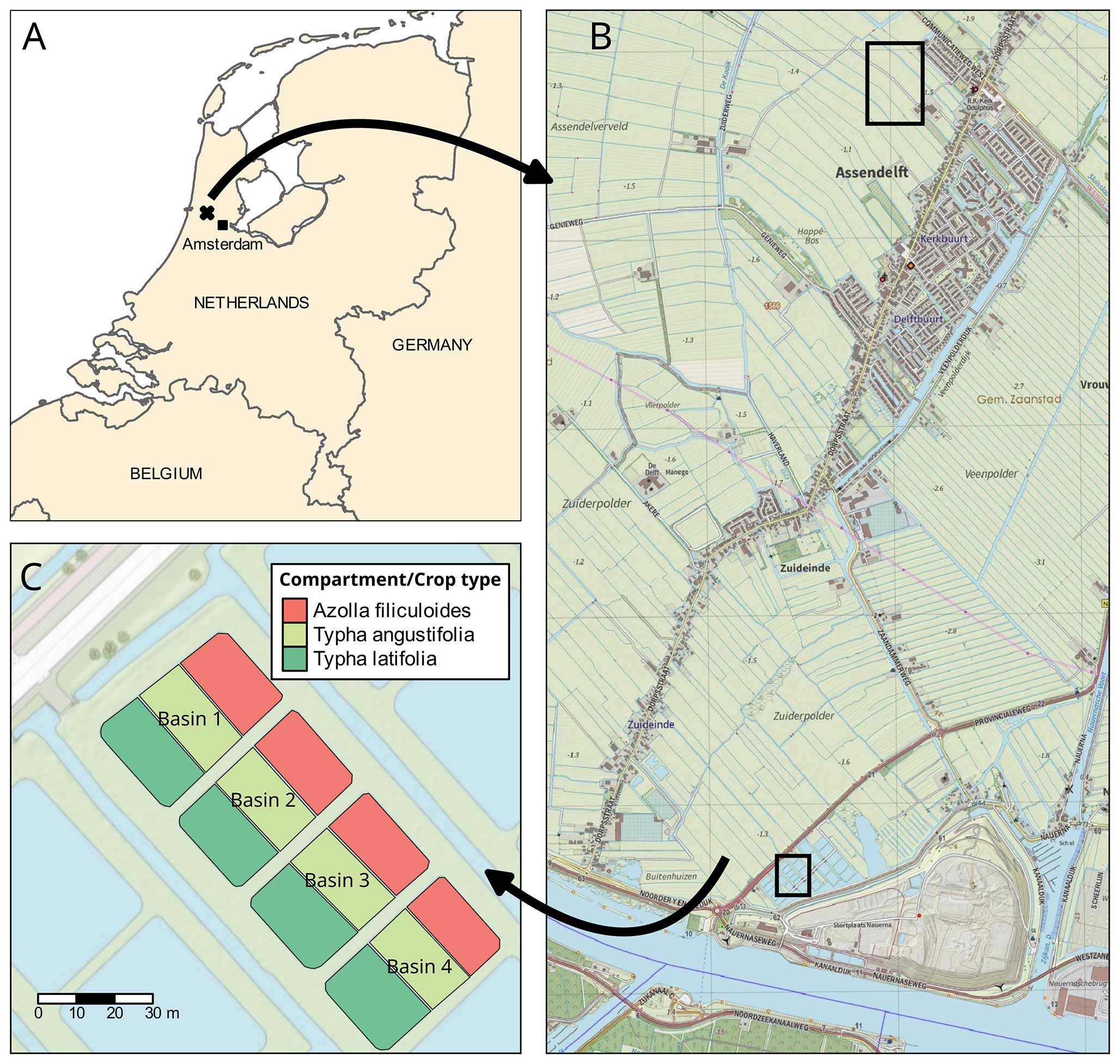
Figure 1(a) Overview of the research area located in the Netherlands (source map: SPOTinfo), with in (b) the paludiculture location in the small lower square and the reference drained fen grassland in the big upper square (source map: GADM). Panel (c) shows basin 2, in which measurements for this research were conducted. (The other basins were used to test treatments that are not discussed in this paper.)
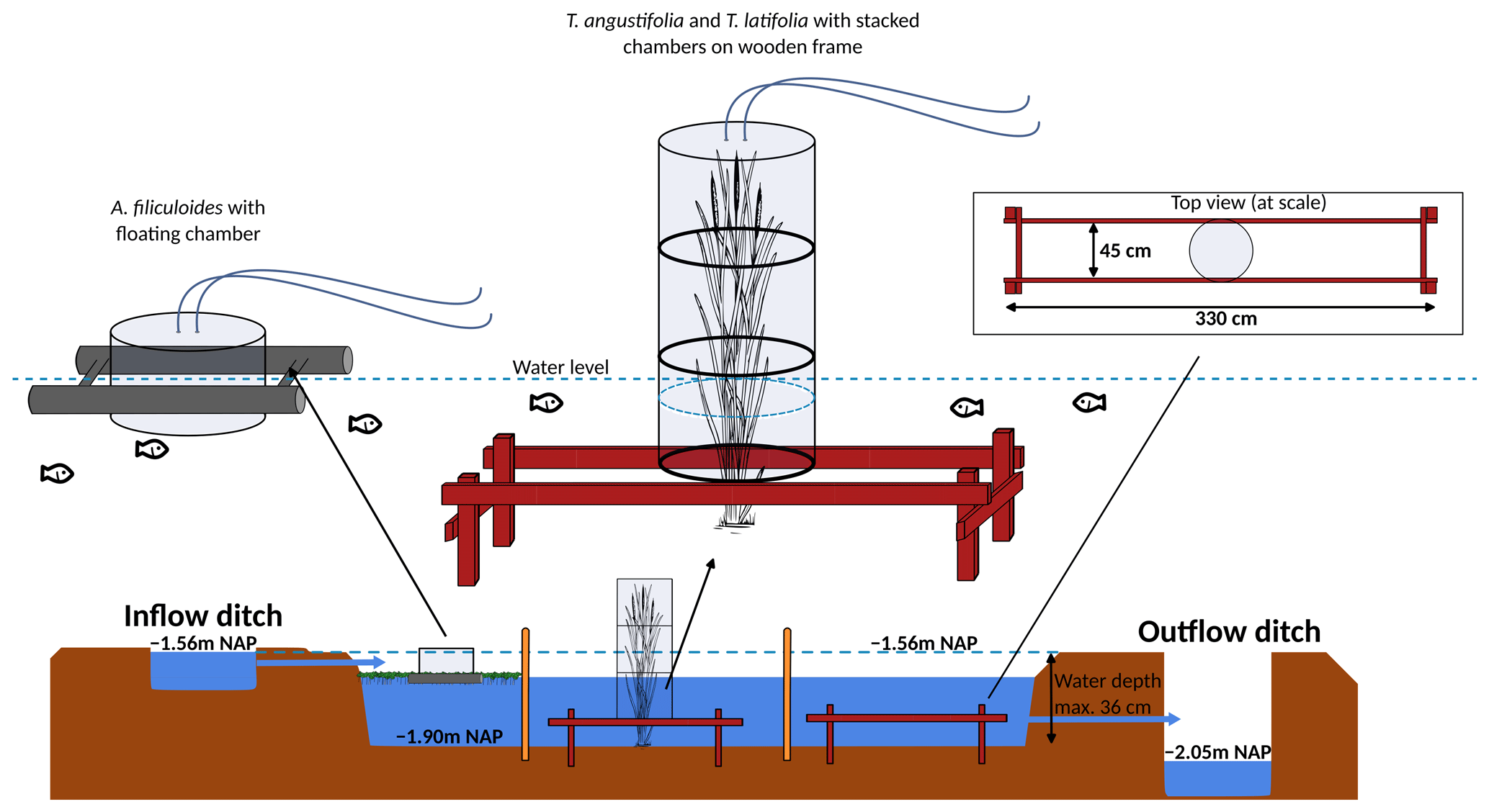
Figure 2Set-up greenhouse gas flux measurement in experimental basin, with on the left the overview for Azolla and in the middle and right for Typha angustifolia and Typha latifolia, respectively. Water tables are relative to Amsterdam Ordnance Datum (NAP).
The reference site in Assendelft (52°28′31′′ N, 4°44′23′′ E) was a managed drained peatland used for dairy farming, where perennial ryegrass (Lolium perenne) is grazed and harvested during the growing season. Although the land management differs from the initial experimental site, they were similar in soil profile with a top layer (∼ 30 cm) of clayey peat and several meters of peat below. In terms of water management, both sites were also similar, with summer groundwater levels around 50 cm below surface. A large research plot of 24×10 m was fenced off, in which CO2 flux measurements were done with automated chambers and many environmental variables (such as water table, soil- and air temperature, and radiation) were monitored from April 2020 onwards. Chamber systems were relocated every 2 weeks at four different positions to minimize the effect of the chamber on temperature and vegetation growth. In 2020, every 4 weeks from 12 May to 29 October, grass was harvested from all chamber subplots and yield was determined at the latest chamber position and from a larger reference area next to the chambers (see Boonman et al., 2022). Fertilization was done with inorganic fertilizers (250 kg N, 108 kg P2O5, and 195 kg K2O ha−1 yr−1) to prevent carbon addition to the soil. Data from the reference site were gathered in the framework of a different project, and more information about the site and measurements can be found in Boonman et al. (2022).
2.2 Flux measurements
In the experimental site, CO2 and CH4 fluxes were measured monthly from March to December 2020 with manual chambers, and five times (March, May, July, September, and October) between the manual measurements with automated chambers aiming to capture diurnal patterns (results are described in Vroom et al., 2024).
For manual chamber measurements in both Typha species, transparent Perspex chambers (diameter 50 cm) were used that could be stacked to match the height of the plants (Fig. 3). The chambers were equipped with a fan powered by a battery. The top part additionally contained a temperature logger and photosynthetically active radiation (PAR) logger (both HOBO onset; Onset Computer Corporation, Bourne, MA, USA). For Azolla, a floating transparent Perspex chamber was used (diameter 29 cm and height 26 cm) equipped with a HOBO temperature logger. PAR was measured with a handheld device outside the chamber (PAR Quantum sensor SKP 215; Skye Instruments, Llandrindod, Wales, UK). Chambers were connected in a closed loop with gas-tight tubing to either a LI-COR 7810 portable GHG analyzer (LI-COR, Lincoln, NE, USA) or a Los Gatos ultra-portable GHG analyzer (ABB; Los Gatos Research, San Jose, CA, USA) that measured CO2, H2O, and CH4 concentrations every second. Measurements were carried out during daytime and lasted 3 min each. Fluxes were alternated between light, darkened (chambers covered with opaque white plastic film), and shaded (chambers covered with plastic shading net, reducing PAR with ∼ 42 %) measurements, to cover the PAR range as much as possible. Per measurement campaign, three light, three darkened, and three shaded measurements were done per species in three replicate locations (total n = 27). The increase in CO2 and CH4 concentrations in the chamber were visually checked for linearity in the field to ensure no ebullition occurred during the measurements. Measurements were redone if high concentration peaks, caused by ebullition, were detected. Fluxes were calculated by taking the linear fit of the concentration change in the first 1–3 min after closing the chamber.
Automated chambers consisted of four Perspex chambers with a diameter of 35 cm and a height of 50 cm. The chambers can be extended up to 150 cm in height to match vegetation height (Fig. 1) and were placed in one vegetation type at a time, measuring 3 d per vegetation type. These chambers were equipped with fans and DS18b50 temperature sensors. Furthermore, they had hinged lids controlled by a connected Raspberry Pi computer (Raspberry Pi Foundation, Cambridge, UK) and were connected with gas-tight tubing in three closed loops to a Los Gatos ultra-portable GHG analyzer. The four chambers were measured in succession by closing the lid of a respective chamber for 2.5 min, followed by 1 min of flushing the chamber and gas analyzer with atmospheric air and then closing the lid of the next chamber, measuring, and flushing. This sequence continued for 3 d in each vegetation type, providing high resolution data including diurnal variations in emissions.
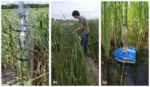
Figure 3Automated chamber (a), manual chamber (b), and bubble trap (c), used for measuring fluxes.
From March till December, ebullitive CH4 fluxes were captured with bubble traps (see Aben et al., 2017) from the three paludicrops. Three bubble traps were installed in each vegetation type (total n = 9). These traps consisted of a small floating foam raft with a funnel (diameter 20 cm) inserted on the bottom part connected to a glass tube above the raft (Fig. 3). To prevent ducks from sitting on the raft, toothpicks were inserted in the foam. A butyl stopper was fitted at the top of each glass tube to enable gas extraction. Gas volume was determined every 1.5–3 weeks by removing the captured gas with a syringe. To determine CH4 concentrations, gas was sampled once a month (in April, May, November, and December) or twice a month (in June and October). CH4 concentrations of 1 mL of diluted gas sample were measured with a Los Gatos ultra-portable GHG analyzer using an open loop of gas-tight tubing.
CO2 fluxes in the reference site (Assendelft) were measured with four automated chambers, connected in a closed loop to a LI-850 CO2 gas analyzer (LI-COR). The chambers had a height of 0.5 m and a diameter of 0.4 m. Every 15 min, each chamber measured for 3 min. (More details about this chamber setup and measurements can be found in Boonman et al., 2022.) CH4 fluxes were not measured in 2020. However, in 2019, CH4 fluxes were captured with the same method and frequency as described for the paludiculture plots. These data showed that CH4 fluxes were close to zero on a yearly basis (−0.04 t CO2 eq. ha−1 yr−1; Gremmen et al., 2022). Therefore, we assumed zero CH4 emissions in 2020.
No flux measurements were done in ditches; therefore, the data only represent fluxes from the (rewetted) land area.
2.3 Partitioning and interpolation of fluxes
Measured net ecosystem exchange (NEE) for CO2 from manual chambers and automated chambers averaged over 30 min were partitioned into gross primary production (GPP) and ecosystem respiration (Reco) by subtracting the Reco based on dark measurements from the shaded and light measurements. With this the Lloyd–Taylor function (Eq. 1; Lloyd and Taylor, 1994) for Reco and the light response curve for GPP could be fitted. The obtained parameters were used for interpolation of GPP and Reco between the measurement campaigns. The Lloyd–Taylor function was defined as
where Rref is respiration at reference temperature (Tref), E0 is the long-term ecosystem sensitivity coefficient, T0 is base temperature between 0 and T (227.13 K; Lloyd and Taylor, 1994), T is the observed temperature (K), and Tref is the reference temperature (K).
E0 was determined by fitting E0 and Rref using the entire dataset, where Tref of 283.15 K was used, T was represented by average soil temperature at 5 cm depth, and the observed Reco were averaged dark or night-time CO2 fluxes per measurement campaign or day. With the gained E0, Rref per measurement campaign or day at a Tref of 283.15 K was determined by inverse of the Lloyd–Taylor function with the average measured dark or nighttime CO2 flux as Reco and the average soil temperature at 5 cm depth as T. Rref was linearly interpolated between the measurement campaigns. Both Rref and E0 were used to calculate Reco for every 30 min with measured soil temperature when data were absent.
Daytime fluxes were partitioned based on the standard procedure as used in, for example, Falge et al. (2001), Veenendaal et al. (2007), and Tiemeyer et al. (2016). GPP was gained from the NEE by subtracting calculated Reco: GPP = NEE − Reco. The parameters α and GPPmax of a hyperbolic light response equation based on the Michaelis–Menten kinetic (Eq. 2) were fitted on the given GPP:
where α is the initial slope of the light response curve, GPPmax is the light-saturated photosynthetic rate, and PAR is the measured photosynthetically active radiation. GPPmax and α were linearly interpolated between the measurement campaigns and used to calculate GPP on a 30 min basis when no data were present.
CO2 partitioning and gap filling (interpolation) was slightly different for the automated chambers on the reference location Assendelft, since the data density was much higher and Reco was determined from nighttime data and calculated for daytime based on the temperature response of the Lloyd–Taylor relation. (For more details see Boonman et al., 2022.) The only difference is the missing data from January to March 2020, since measurements started in April 2020. Reco for this period was estimated by fitting the Lloyd–Taylor function on the winter period January to March for 2021–2023 and using the gained Rref and E0 with the measured soil temperature for the period January to March 2020. To estimate GPP in 2020, we used the monthly average of the parameter α and the GPPmax for January to March for 2021, since first harvest of 2020 and 2021 were similar, together with measured PAR for January to March 2020.
For CH4 there is no standard interpolation procedure, and therefore a part of this study aimed to find the best relation between environmental variables and diffusive fluxes. Many studies show that temperature is one of the best predictor variables for CH4 fluxes (Kroon et al., 2010; Turetsky et al., 2014; Irvin et al., 2021). Other mentioned predictors are water table (which does not fluctuate in our study and therefore is not relevant) and vegetation. We choose to only use temperature to interpolate our data and base that on the same principle as the interpolation of Reco with the Lloyd–Taylor function: we assume that influences of factors other than temperature, such as vegetation, are captured in the mean measured CH4 flux every 2–3 weeks and are linearly changing over time. We found that the best predictor variables for CH4 fluxes were soil temperature for Typha and water temperature for Azolla, with an exponential relation (see Sect. 3.3 “Methane fluxes”). We used the mean measured CH4 flux per campaign, calculated this back to a reference temperature of 10 °C with the gained temperature relation (Fig. 7), linearly interpolated these reference emissions, and calculated the actual emission with the measured temperature and the temperature relation from this reference emission.
2.4 Vegetation measurements
To estimate the biomass of Typha spp. per measurement campaign, average biomass per plant height was related to number of plants and plant height per campaign. For this, 10 living shoots were harvested for each species outside of the measurement plots in September 2020. These shoots were dried at 70 °C for 72 h, and dry weight per centimeter of biomass was calculated. This was then multiplied by the number of living shoots and the average shoot height in each subplot to estimate the biomass at each measurement campaign (Fig. A1 in the Appendix). For the C-export term, the average number of dead stems was subtracted from the number of living stems from the measurement plots, and with the above-described relation it was used to determine the extra amount of biomass produced in 2020. This was called C-export since this could have been the potential net term of carbon loss by harvest.
For Azolla, biomass was not directly estimated, only the biomass cover per measurement campaign (Fig. A1).
2.5 Sample collection
Soil samples of the experimental site, before topsoil removal and rewetting, were collected in March 2017. Samples were collected at five locations, divided over the area where the four experimental paludiculture basins were planned, at a depth of 0–10, 10–20, and 20–30 cm below surface level. After topsoil removal and rewetting, additional samples were collected in November 2018 in the four experimental basins. Here, five samples of the inundated topsoil (0–10 cm) were collected in each compartment of the four basins, after which the samples were pooled per compartment before analysis. All samples were stored in airtight plastic bags at 4 °C until further analysis.
Surface water and pore water samples were collected monthly directly after manual chamber measurements in the experimental basins as well as inflow- and outflow ditches. Surface water samples were taken by hand in the inlet water ditch and each compartment (n=1 per compartment/ditch). Pore water was collected anaerobically with a 60 mL syringe attached to a ceramic cup via gas-tight tubing, which was installed in the top 15 cm of the sediment in each respective compartment. Additional pore water samples for dissolved CH4 and sulfide (H2S) were collected by attaching a gas-tight pre-vacuumed 12 mL glass exetainer (containing 1 mL of 0.5 M HCl to stop microbial activity; Labco, Lampeter, UK) via a hypodermic needle to the gas-tight tubing. The exetainers were stored upside down to minimize the risk of gas leakage. All samples were stored at 4 °C until further analysis.
2.6 Soil analysis
Two aluminum cups (40.5 mL) were filled with fresh soil and weighed before and after drying at 60 °C for > 48 h to obtain the wet weight and bulk density, respectively. Thereafter, one cup with dried soil was incinerated (4 h at 550 °C) and weighed again to determine organic matter (as loss on ignition). Total phosphorus (P), iron (Fe), and sulfur (S) content were determined by digesting 200 mg of homogenized finely ground soil with 5 mL 65 % HNO3 and 2 mL H2O2 in a microwave (Ethos Easy; Milestone, Sorisole, Italy). Samples were then diluted to 100 mL with demineralized water and analyzed using inductively coupled spectrometry axial plasma observation, sea-spray nebulizer, 1300 W, 12 L min−1 (ICP-OES ARCOS MV; SPECTRO Analytical Instruments, Kleve, Germany). Plant-available extractable inorganic nitrogen was determined by incubating 17.5 g of fresh soil with 50 mL of 0.2 M NaCl for 2 h with 105 rpm and at room temperature. After determining the pH (PHC101 probe connected to HQ440d; Hach, Düsseldorf, Germany), the extract was collected using soil moisture samplers (Rhizon SMS; Eijkelkamp, Giesbeek, the Netherlands) and analyzed colorimetrically for nitrate (NO) and ammonium (NH) on an auto-analyzer III (Seal Analytical; Norderstedt, Germany) using hydrazine sulfate and salicylate reagent, respectively. Plant-available extractable phosphorus (Olsen P) was determined by incubating 3 g of dried homogenized finely ground soil with 60 mL of 0.5 M NaHCO3 at pH 8.5 for 30 min with 105 rpm at room temperature. The pH of the medium was adjusted before incubation by adding NaOH when necessary. The extracted medium was diluted 10 times with demineralized water and stored at 4 °C until further analysis on ICP-OES as described above.
2.7 Surface water and pore water analysis
The pH was measured using a standard electrode connected to a radiometer (model TIM840; Radiometer, Copenhagen, Denmark). The total inorganic carbon (TIC) concentration was determined by injecting a known amount of sample into an infra-red gas analyzer (ABB Advance Optima IRGA), after which the concentrations of CO2 and HCO were calculated based on the pH equilibrium. Concentrations of nitrate (NO) and ammonium (NH) were determined colorimetrically on an auto-analyzer as described above. Chloride (Cl−) and phosphate (PO) concentrations were determined colorimetrically on a Bran + Luebbe (Norderstedt, Germany) auto-analyzer III system using, respectively, mercury(II)cyanide and ammonium molybdate/ascorbic acid as the reagent. Acidified samples (0.1 mL 65 % HNO3) were analyzed for total Fe, total P, and total S on ICP-OES as described above. After equilibrating to atmospheric pressure with N2 gas, the concentrations of methane (CH4) and sulfide (S2−) were measured in the headspace of the exetainers by injecting a known volume of sample into a 7890B gas chromatograph (Agilent Technologies, Santa Clara, CA, USA) equipped with a Carbopack BHT100 (Supelco, Bellefonte, PA, USA) glass column (2 m and i.d. 2 mm), flame ionization detector (FID) and flame photometric detector (FPD). Concentrations of dissolved organic carbon (DOC) were measured on a TOC-L CPH/CPN analyzer (Shimadzu, Kyoto, Japan) after acidification with HCl to remove DIC.
2.8 Environmental variables
Surface water and groundwater levels were calculated based on hourly measurements of atmospheric pressure (Baro-Diver; Eijkelkamp, Giesbeek, the Netherlands) and water pressure at a known depth (Cera-Diver; Eijkelkamp, Giesbeek, the Netherlands). Air temperature was also measured hourly (using Baro-Diver). Soil and water temperatures were monitored at a 2 min interval (HOBO S-TMB temperature probe connected to an H21-USB station; Onset, Bourne, MA, USA). Water temperature was measured in the T. angustifolia compartment and soil temperature was measured at 5 cm depth in each compartment. PAR was monitored at a 2 min interval at 3 m above water level using a HOBO S-LIA-M003 PAR sensor connected to an H21-USB station (Onset).
3.1 Environmental conditions
The study was conducted in 2020, which was a slightly warmer (+0.9 °C) year than the 10-year average of 2001–2020 (Royal Netherlands Meteorological Institute KNMI). The yearly average precipitation was very similar to average (862 mm in 2020), but the summer period (June to September) was dryer (337 vs. 474 mm).
The seasonal dynamics are clearly visible in all variables. The groundwater table of the reference site reaches a minimum of −86 cm in August and was on average −38 cm in 2020 (Fig. 4). The water table in the paludiculture basin was kept more or less constant at +18 cm. Due to this water layer, the soil temperature fluctuations in the paludiculture basin were much more dampened than within the reference site (Fig. 4).
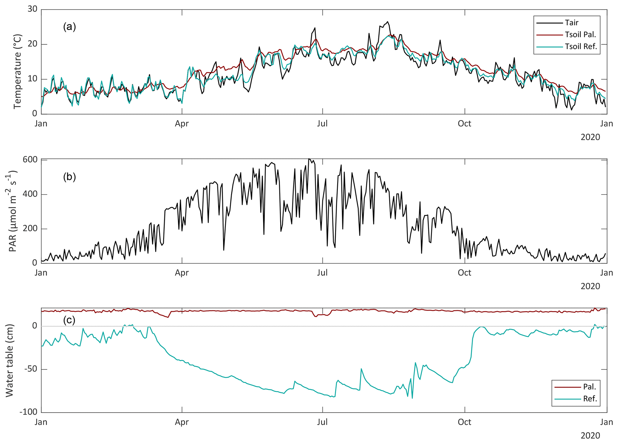
Figure 4(a) Air temperature (Tair) and site-specific soil temperature (Tsoil) for paludiculture site (Pal.) and reference site (Ref.), (b) photosynthetically active radiation (PAR), and (c) (ground)water table for the paludiculture site and reference site.
3.2 Effect of rewetting and plant growth on surface and pore water chemistry
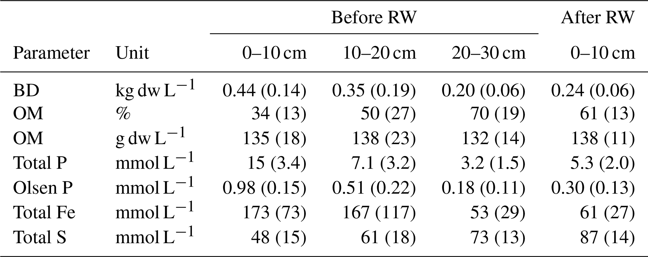
After topsoil removal, the total amount of organic matter remained the same in the upper soil layer, but bulk density in the top layer (0–10 cm) was reduced by about 50 % (Table 1). Also, total phosphorus and total iron decreased quite drastically, by about 65 %, whereas total sulfur increased by 81 %, which could lead to an increase in (toxic) free sulfide in the root zone (Table 1). Assuming 58 % of the organic matter content (OM) was carbon (C) (van Bemmelen factor), the removal of ∼ 20 cm of the topsoil resulted in the displacement of approximately 15.8 kg C m−2.
Table 1Soil properties of bulk density (BD), organic matter content (OM), total phosphorus (Total P), plant-available phosphorus (Olsen P), total iron (Total Fe), and total sulfur (Total S) before rewetting (RW) and topsoil removal in 2017 (n=5), and after rewetting and topsoil removal in 2018 (n=12). Because ∼ 20 cm of topsoil is removed, the depth 0–10 cm after RW corresponds to the soil layer 20–30 cm before RW. The numbers in parentheses denote the standard deviations.
Surface water and pore water chemistry were measured during the whole measurement period in 2020 (Figs. 5 and 6). Surface water ammonium (NH) and nitrate (NO) concentrations were relatively low throughout the growing season (< 25 and < 8 µmol L−1, respectively). The concentration of phosphate (PO) was also low throughout the growing season in both Typha compartments (< 2.5 µmol L−1) but increased in the inlet water ditch to 9.2 µmol L−1 in July. The pH varied between 7 and 8.6, with the highest values from May to September and the lowest in winter (Table A1). The chloride (Cl−) concentration also showed a clear seasonal pattern, with relatively low concentrations in winter (∼ 20 mmol L−1 in February) and high concentrations in summer (∼ 60 mmol L−1 in August 2020). Total sulfur was highly variable over time but was generally lower in both Typha compartments (221–887 µmol L−1 in T. angustifolia and 127–432 µmol L−1 in T. latifolia) compared with the Azolla compartment (387–1291 µmol L−1) and the water inlet ditch (495–1414 µmol L−1).
In the pore water, NH and total P concentrations were low throughout the year in both Typha compartments (< 30 and < 4.4 µmol L−1, respectively). In the Azolla compartment, however, NH was substantially higher with concentrations ranging from 130 µmol L−1 in July 2020 to 650 µmol L−1 in September 2020. Total P increased from 10 µmol L−1 in March to 50 µmol L−1 in October. The Cl− concentration in the pore water showed a seasonal pattern as well, with 20–40 mmol L−1 in March 2020 to 45–70 mmol L−1 in October 2020. In the Azolla compartment, pore water was very iron (total Fe)- and sulfur (total S)-rich in March and April 2020 (> 3000 and > 1000 µmol L−1, respectively; Table A2) but dropped to concentrations similar to those of both Typha compartments during summer. Sulfide (S2−) concentrations in the pore water were very low (< 0.2 µmol L−1) throughout the year in all three compartments (Table A2).
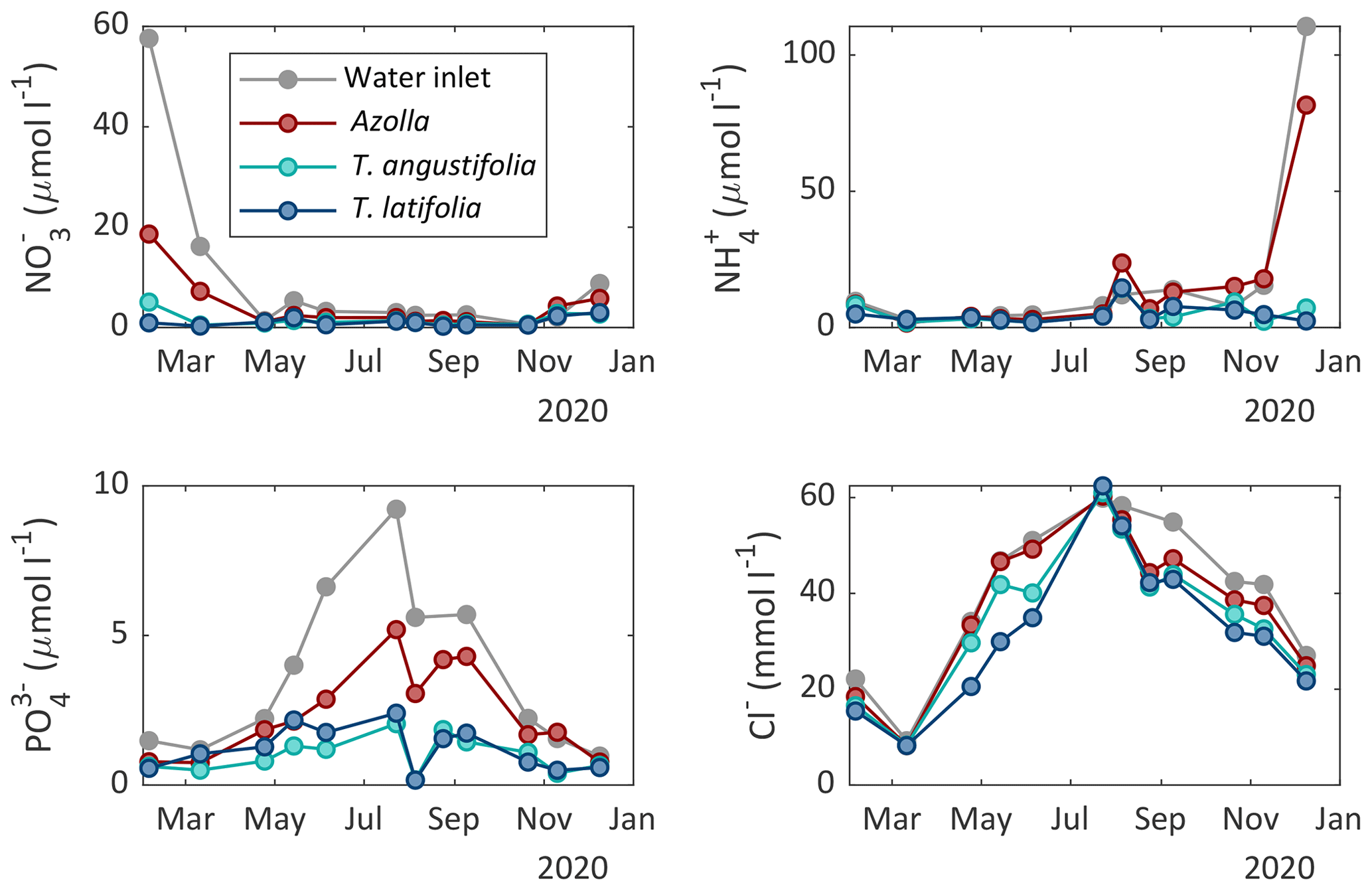
Figure 5Surface water chemistry of nitrate (NO), ammonium (NH), phosphate (PO), and chloride (Cl−) measured in the different compartments of the three paludicrops and in the water inlet ditch at different moments in time.
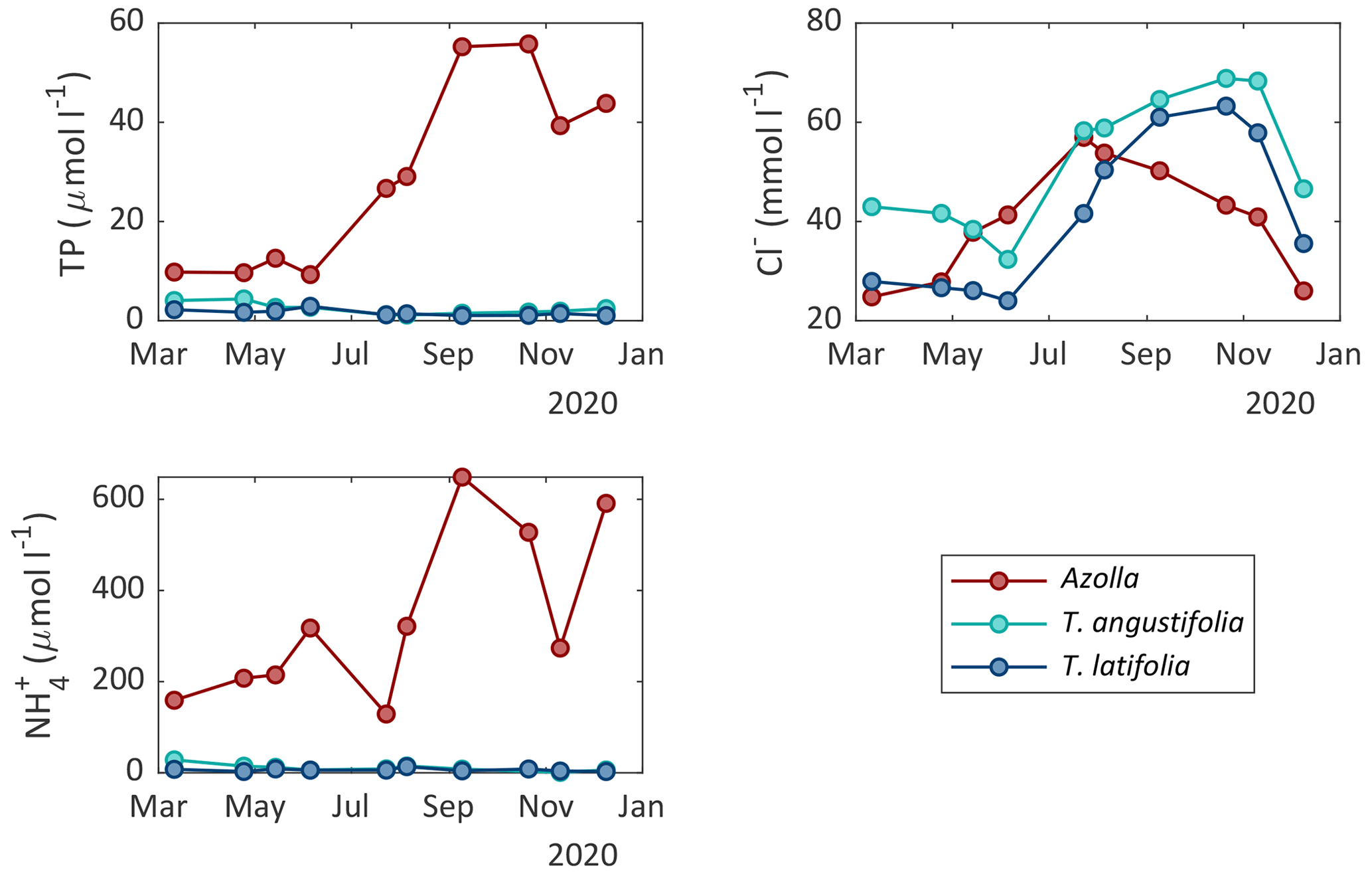
Figure 6Pore water chemistry of ammonium (NH), total phosphorus (TP), and chloride (Cl−) measured in the soil of the different compartments of the three paludicrops at different moments in time.
3.3 Methane fluxes
Diffusive CH4 fluxes were measured with chambers and ebullition with bubble traps for all three paludicrops. For interpolating CH4 fluxes to come to a yearly budget, relations with environmental variables were analyzed for the three paludicrops. Diffusive CH4 fluxes from T. latifolia and T. angustifolia showed the strongest correlation with living above-ground biomass (R2 = 0.78 and 0.63, respectively). However, this variable is not useful for interpolation, since we do not have biomass data between the measurement campaigns. Soil temperature was the second-best explanatory factor for CH4 emissions for both Typha species (R2 = 0.63 for T. latifolia; R2 = 0.58 for T. angustifolia), and had a very strong correlation with above-ground biomass (R2 = 0.94 for T. latifolia and R2 = 0.95 for T. angustifolia). For Azolla, water temperature correlated slightly better (R2 = 0.45) than soil temperature (R2 = 0.37). Therefore, for Typha we used soil temperature and for Azolla water temperature for interpolating the diffusive CH4 fluxes as showed in Fig. 7b. (For a more detailed description of the interpolation, see Sect. 2.3.)
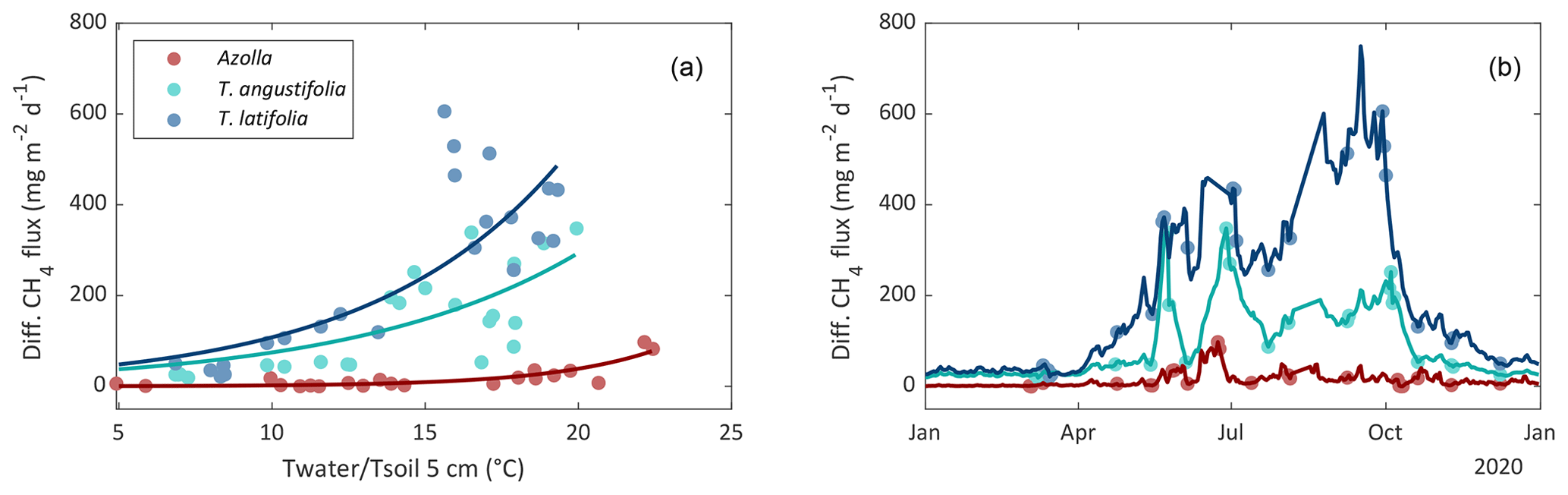
Figure 7Relation between daily mean diffusive CH4 flux with water temperature (Azolla) or soil temperature at 5 cm depth (Typha angustifolia and Typha latifolia) (a). Measured (dots) and interpolated (lines) diffusive CH4 flux by using the temperature relation (b).
Ebullition measurements were considered as the average ebullitive flux between the sampling moments. This created a continuous data series, except for January to February where there were no measurements yet. Ebullitive fluxes for January to February were assumed to be the same as for March.
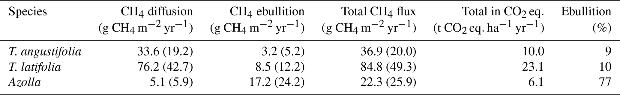
The yearly sum of CH4 flux was highest for T. latifolia and lowest for Azolla, with the highest absolute and relative contribution of ebullition for Azolla (Table 2).
Table 2Total CH4 flux for 2020 for T. angustifolia, T. latifolia, and Azolla. Total flux consists of diffusive flux and ebullition flux. The numbers in parentheses denote the standard deviations, representing the variation between the measurement replicates. For the calculation of CH4 fluxes in CO2 equivalent (CO2 eq.), a GWP100 of 27.2 is used (IPCC, 2021).
3.4 Carbon dioxide fluxes
CO2 fluxes always reflect a combination of different processes: daytime uptake of CO2 by plant photosynthesis (GPP), and ecosystem respiration (Reco) as the sum of plant respiration for maintenance and growth (autotrophic respiration) as well as soil respiration (heterotrophic respiration). Reco showed large differences between the different paludicrops and over the seasons (Fig. 8). For the three different species, the total year sum of CO2 was the highest for T. latifolia, but Reco was still around half of that from the reference site (Table 3). T. latifolia had a higher GPP compared with T. angustifolia, but this could only partly explain the difference in Reco. Azolla clearly had the lowest GPP (and thus biomass production) and the lowest Reco. However, in relation to the GPP, Reco was relatively high, resulting in the lowest net uptake of CO2 (NEE) (Table 3).
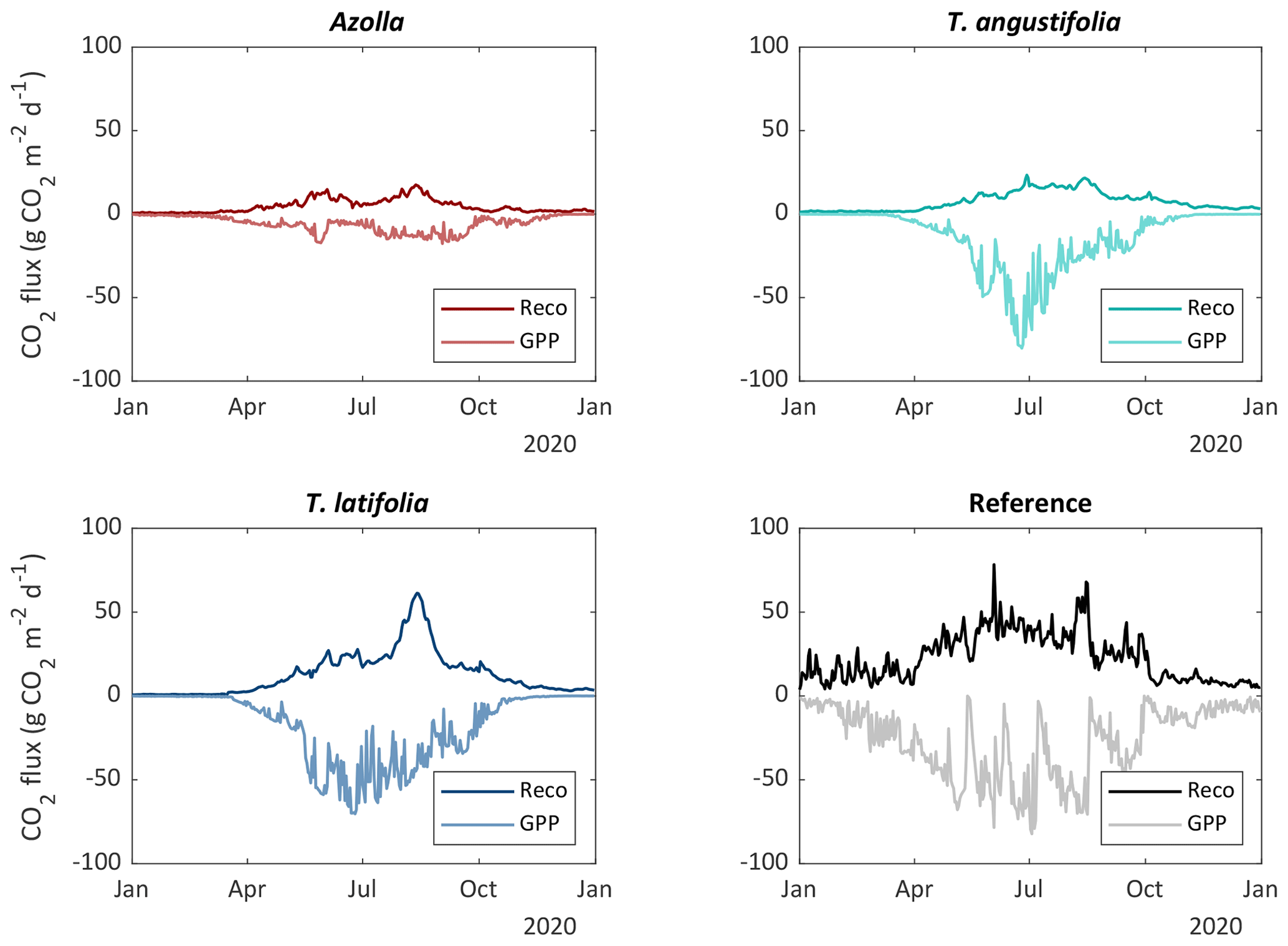
Figure 8Estimated daily average ecosystem respiration (Reco) and gross primary production (GPP) for the three paludicrops and the drained reference site.
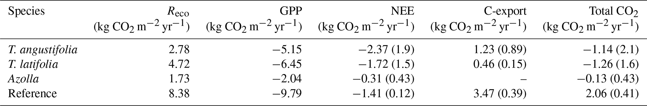
To derive an annual CO2 balance, the fluxes were interpolated (see Sect. 2.3) over the entire year (Fig. 8). To be conservative with the CO2 balance, it is assumed that all harvested biomass will be decomposed at some point, and this was therefore converted to CO2 (as C-export term) and added to the NEE to come to the complete CO2 balance. Biomass could, however, be stored sustainably in, for instance, building material, which would reduce the total CO2 flux. On the other hand, if biomass is used for fodder, carbon could be released as CH4 again, increasing the total greenhouse gas flux. This is not considered within our balances. Harvested biomass for T. latifolia and T. angustifolia at the end of 2020 was estimated to be 8 and 11 t dm ha−1 yr−1, respectively. The harvested biomass was corrected for the biomass that was left in the previous year (not harvested), to avoid double counting. In total, we observed that the net uptake of CO2 was greater than the yield, meaning that the CO2 balance results in a CO2 uptake of the system for all crops, with the highest uptake (−1.26 kg CO2 m−2 yr−1) for T. latifolia and lowest uptake for Azolla (−0.13 kg CO2 m−2 yr−1) (Table 3).
Table 3Yearly interpolated CO2 fluxes consisting of ecosystem respiration (Reco), gross primary production (GPP), net ecosystem exchange (NEE), carbon removed from harvest (C-export), and the sum of NEE and C-export (Total CO2). The numbers in parentheses denote the standard deviations, representing the variation between the measurement replicates. For Typha C-export two samples were taken, so no standard deviation could be determined.
3.5 Total greenhouse gas balance
For the greenhouse gas (GHG) balance, both CO2 and CH4 emissions in CO2 equivalents (CO2 eq.; GWP100 of 27.2; IPCC, 2021) were summed up. For the reference site, we did not measure CH4 fluxes in 2020; however, CH4 fluxes were assumed to be zero based on CH4 flux measurements on the same site in 2019 (Gremmen et al., 2022).
For the paludicrops, only T. angustifolia had a higher uptake of CO2 (also considering C-export) than the CH4 in CO2 eq. that was emitted, making it a net GHG sink (−1.4 t CO2 eq. ha−1 yr−1). With the other two species, CH4 emissions were higher than CO2 uptake, with higher emissions for T. latifolia (10.5 t CO2 eq. ha−1 yr−1) than for Azolla (2.9 t CO2 eq. ha−1 yr−1) (Fig. 9). Nevertheless, all paludicrops had a lower net GHG emission than the reference site (20.6 t CO2 eq. ha−1 yr−1). However, in this balance the potential CO2 emission from the topsoil removal from the paludiculture site (557 t CO2 ha−1) is not accounted for.
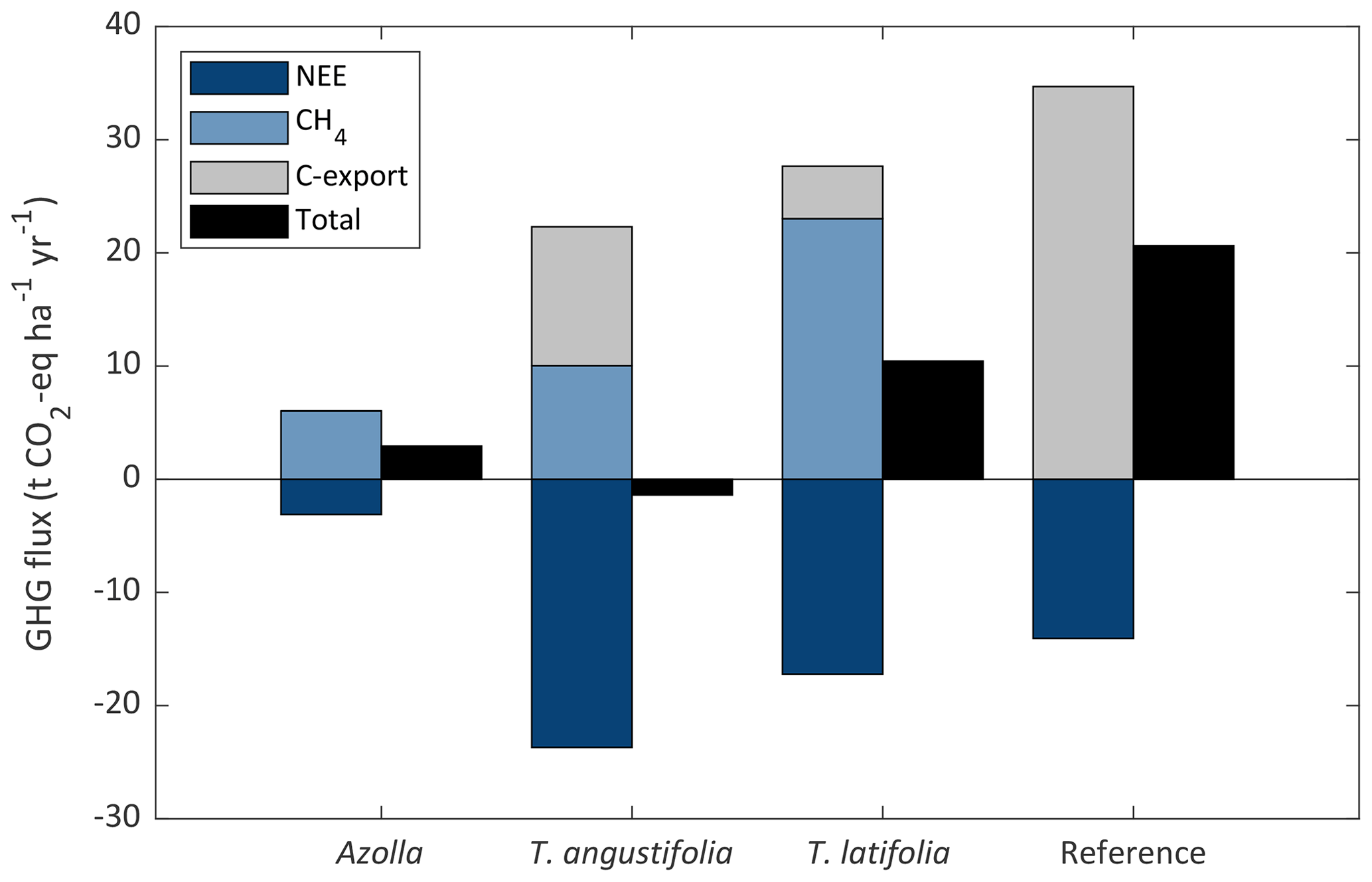
Figure 9Greenhouse gas (GHG) balance for the three paludicrops and the reference site. GHG balance consists of net ecosystem exchange of CO2 (NEE), carbon removed by harvest (C-export), and CH4 flux (consisting of ebullition and diffusive fluxes) expressed in CO2 equivalent (GWP100 of 27.2; IPCC, 2021), as well as the total net flux as the sum of the three terms. Typha yield was corrected for the biomass that was left in 2019; therefore, it does not represent the potential yield from the Typha fields.
Since CH4 has a relatively short lifetime in the atmosphere (it reacts with hydroxyl radicals to form CO2 and water vapor), the contribution of CH4 to the radiative forcing of our planet has different behavior over time than CO2. This creates a complex trade-off between reducing CO2 emissions from drained peatlands vs. rewetting and creating CH4 emissions in the long term (Günther et al., 2020). To visualize this, we used the radiative forcing model of Günther et al. to see what the long-term effect is of rewetting and topsoil removal for paludiculture compared with the reference site for CO2 and CH4. In this case we assumed that the current measured CO2 and CH4 fluxes will continue until the end of the century and that the removed carbon from the topsoil will be decomposed to CO2 within 27 years (assuming the CO2 emissions will be the same as from the reference site). We also assumed that the harvested biomass (yield) is decomposed again to CO2 within that same year. The total radiative forcing is the sum of the contribution from CH4 emissions, CO2 from topsoil removal, and net CO2 flux (NEE + yield), and it is calculated for an area of 220 000 ha (area of arable drained peatlands in the Netherlands). The results show that in the first decades the total radiative forcing for all paludicrops is higher than for the reference site, due to the combination of increasing radiative forcing from CH4 emissions and CO2 emissions from topsoil removal (Fig. 10). After 27 years, the emissions from topsoil removal stops and radiative forcing from CH4 emissions steadily flattens off. From the year 2063, radiative forcing for (coincidently) both Azolla and T. angustifolia becomes lower than for the reference site. For T. latifolia this is not going to happen until the year 2113. Eventually, with the additional flux of topsoil removal, T. latifolia has the highest impact on the radiative forcing in the year 2100: W m−2 compared with W m−2 for Azolla, W m−2 for T. angustifolia, and W m−2 for the reference site. Topsoil removal contributes to that with about W m−2 for the three paludicrops.
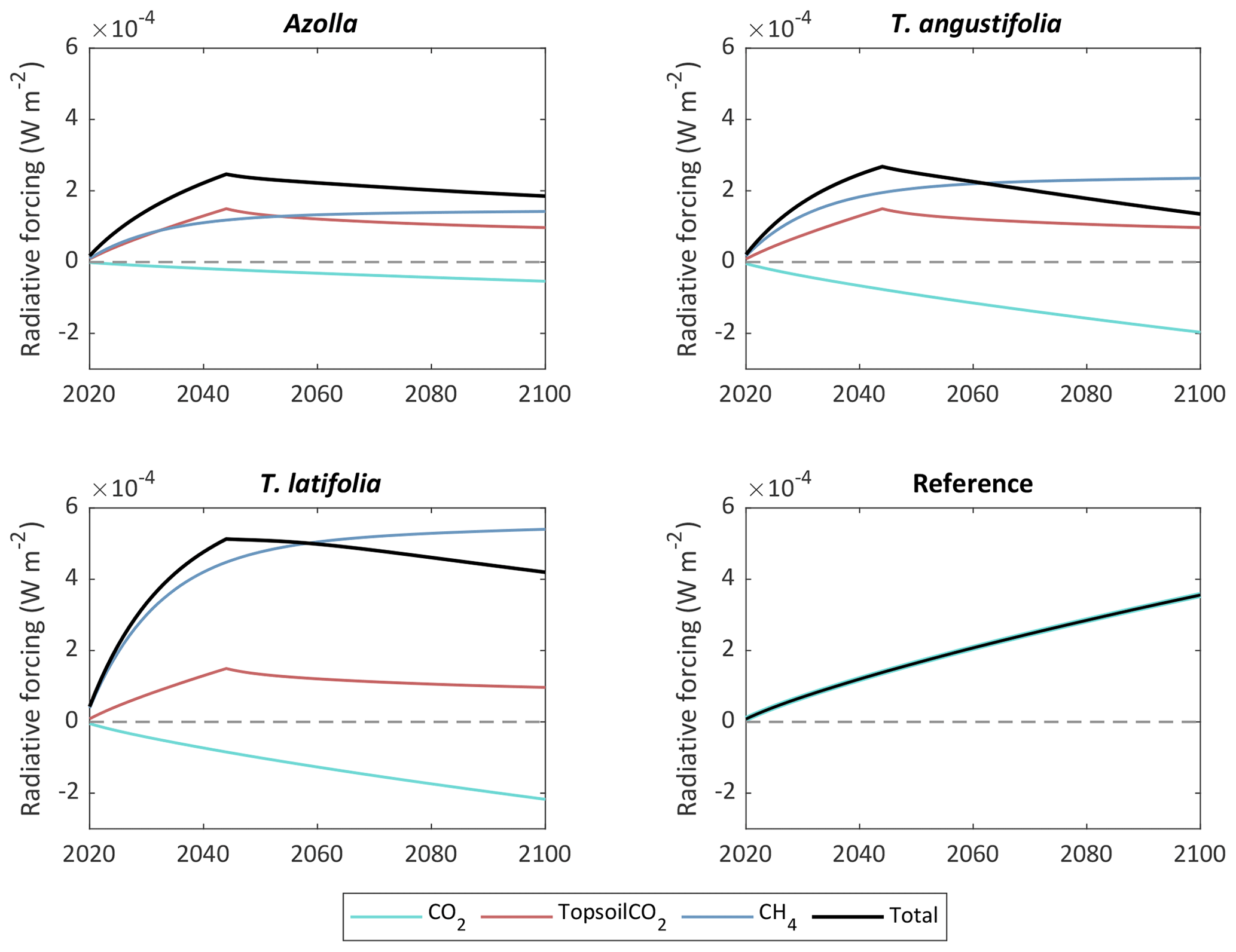
Figure 10Contribution of paludicrops and reference site to radiative forcing for CO2 flux (NEE + yield), estimated CO2 emissions from topsoil removal, and CH4 emissions. The topsoil is assumed to be completely decomposed within 27 years. The radiative forcing is calculated for a land surface area of 220 000 ha, which is the area of drained arable peatlands in the Netherlands.
4.1 Differences in CH4 flux of the three paludicrops
We found large differences in diffusive and ebullitive CH4 fluxes from the three paludicrop species. The differences in CH4 fluxes, with the lowest diffusive and highest ebullitive fluxes for Azolla, can be well explained by the differences in growth forms and species-specific characteristics. (A more thorough discussion of the effects of these plants on CH4 emissions can be found in Vroom et al., under review.) Briefly, Azolla, a free-floating plant without roots in the soil, neither releases root exudates to the sediment nor transports sediment CH4 to the atmosphere. Moreover, radial oxygen loss (ROL) from roots can lead to oxidation of up to 70 % of the produced CH4 (Kosten et al., 2016). This may explain the relatively low CH4 diffusion from Azolla, which has been found for other free-floating species before (Attermeyer et al., 2016). On the other hand, CH4 emissions by ebullition are still substantial, probably due to the release of dead roots and root exudates to the water, providing carbon for methane production. In the case of Typha, plant mediated transport is substantial (Bendix et al., 1994; Yavitt and Knapp, 1998; White and Ganf, 2000) and CH4 production in the sediment can be increased by the supply of carbon through the roots as root exudates, which are an important source for CH4 production (Bastviken et al., 2023). The plant transport of CH4 causes the CH4 concentration in the soil to decrease, which leads to a lower ebullition flux (Van der Nat et al., 1998; Grünfeld and Brix, 1999; Van den Berg et al., 2020). So, although rates of methane production may be higher due to the supply of easily degradable carbon, which will increase over the course of the season as the plants grow larger (Joabsson and Christensen, 2001), the build-up of CH4 in the sediment will remain low. Lower emissions from T. angustifolia than T. latifolia may be explained by the greater ability of T. angustifolia to build up pressure in the stem and higher ROL rates compared with T. latifolia (Bendix et al., 1994; Matsui Inoue and Tsuchiya, 2008), resulting in higher rates of methane oxidation (Bendix et al., 1994). Additionally, in 2020, 90 % of T. latifolia had been damaged by the Webb's Wainscot and/or the Bulrush Wainscot, which may have reduced pressurized flow (Armstrong et al., 1996).
The total CH4 emission in 2020 for T. latifolia was high, both relative to the other species and in absolute terms (84.8 g CH4 m−2 yr−1). Emissions were around a factor ∼ 1.7 higher than what was found in a similar experiment in the Netherlands (Buzacott et al., 2023), but the same magnitude was found in a boreal lake in Canada (Desrosiers et al., 2022). However, Rey-Sanchez et al. (2018) show even higher emissions from a natural system in the USA than what we found (292 g CH4 m−2 yr−1). They hypothesize that the high fluxes could be attributed to high DOC input. This could also be the case in our site, as high TOC values (5.3 mmol L−1; Table A1) were found in the inflow ditch water. Another reason could be plant stress factors, like salinity level and herbivory, resulting in enhanced die-off of plant material. Both factors could lead to higher substrate availability for CH4 production. T. angustifolia was less affected by herbivory and has a higher salt tolerance than T. latifolia (McMillan, 1959).
The lower CH4 emissions for T. angustifolia compared with other rooting wetland plants was also found in another study, where fluxes from Phalaris and Phragmites were a factor 1.7 and a factor 2 higher, respectively (Maltais-Landry et al., 2009). Absolute CH4 emissions from T. angustifolia vary strongly from ∼ 11 g CH4 m−2 yr−1 in a constructed wetland (Maltais-Landry et al., 2009), to ∼ 176 g CH4 m−2 yr−1 in a natural wetland in Canada (Strachan et al., 2015), compared with our 36.9 g CH4 m−2 yr−1. But not many studies were found.
For Azolla, all studies on CH4 fluxes we found were conducted in combination with rice growth. These studies show in general a decrease in CH4 emissions with the addition of Azolla to rice paddies (Bharati et al., 2000; Liu et al., 2017; Xu et al., 2017; Kimani et al., 2018). This is in line with our observations, where we found a factor 1.7–3.8 lower emissions from Azolla compared with Typha.
Overall, our measured CH4 fluxes were high despite the topsoil removal and the brackish conditions, which were expected to reduce CH4 production, due to the removal of easily degradable carbon (Harpenslager et al., 2015; Quadra et al., 2023) and the reducing effect of salinity on CH4 production (Van der Gon and Neue, 1995; Minick et al., 2019), respectively.
4.2 Greenhouse gas balance
Paludiculture reduced the net CO2 balance (including C-export) to a large extent compared with the reference site, going from a net source (+20 t CO2 ha−1 yr−1) to a net sink (−1.3 t CO2 ha−1 yr−1 Azolla, −11.4 t CO2 ha−1 yr−1 T. angustifolia, and −12.6 t CO2 ha−1 yr−1 T. latifolia). This shows that the rewetting was effective in stopping peat oxidation. Adding the CH4 emission in CO2 eq. also resulted in a lower GHG balance for the paludicrops compared with that of the reference site. It is uncertain to what extent the carbon storage measured in the Typha species will continue in the future. As the species were introduced in the years before (2018–2019), it is likely that there is still biomass build-up, like rhizomes, which will come to a steady state and reduce the net uptake. In the literature, lower uptake values for Typha were found, like the range of NEE of −4 to +5 t CO2 ha−1 yr−1 from a rewetted fen in Belarus (Minke et al., 2016), compared with our −24 and −17 t CO2 ha−1 yr−1 for T. angustifolia and T. latifolia, respectively. With Azolla the biomass completely disappeared by the end of the measurement year (die-off due to herbivory) and the net CO2 emission was close to zero. From the growth rate observed at the same field site 1 year later, the expected biomass in a growing season could potentially reach 23–35 t dm ha−1 yr−1 (Gremmen et al., 2022). For Typha, herbivory occurred more in T. latifolia, resulting in higher biomass die-off, which most likely caused more respiration than in T. angustifolia.
The C-export term in Typha contributes to the net CO2 balance with about 27 %–51 % (Table 3). This term is, however, not the C from the total produced biomass, since dead biomass from the previous year was subtracted to make the balance right. Yields of 10–25 t dm ha−1 yr−1 can be possible (Geurts and Fritz, 2018), while our site showed 8 (T. latifolia) to 11 (T. angustifolia) t dm ha−1 yr−1.
The yield term assumes that all harvested carbon is decomposed to CO2 again. This is the case if biomass is burned or used as fodder (although C-emissions can also be in the form of CH4 in this case), but if biomass is used sustainably for long-term storage, such as building material, this C-export should not be accounted for in the carbon/GHG balance. However, to know the exact GHG effect of biomass storage, a life cycle assessment is needed to account for all other emission terms. De Jong et al. (2021) estimated that using Typha as insulation material, emissions from cultivating and processing Typha would be 9.7 t CO2 ha−1 yr−1, which almost compensates for the biomass harvest in T. latifolia. They also concluded that the largest GHG gain is in reducing the peat oxidation, and not in the biomass use.
When taking into account the impact of topsoil removal on the carbon balance, the perspective changes substantially. If all the carbon that is removed from the top 20 cm (15.8 kg m−2) is not stored under anoxic conditions, an amount of 557 t CO2 ha−1 will be released over the period needed to decompose that carbon. That is the same amount the reference site is emitting in 27 years. With the radiative forcing calculation for the different paludicrops (Fig. 10), topsoil removal is the largest contributor for T. angustifolia and around half of the contribution for Azolla by 2100. Therefore, if topsoil removal is applied, one should consider the potentially large CO2 emissions associated with topsoil decomposition. Additionally, Quadra et al. (2023) show that only 5 cm of topsoil removal might be sufficient to significantly reduce CH4 emissions, suggesting that careful consideration of the amount of topsoil removal is warranted.
The impacts of CO2 and CH4 terms on radiative forcing (global warming) do not behave the same over time. With continuous emission, CH4 in the atmosphere will reach equilibrium such that the contribution to radiative forcing stabilizes, while continuous CO2 emissions causes always increasing radiative forcing. The CO2 emissions from topsoil removal will only last until all the organic carbon is decomposed. We illustrate this in Fig. 10 by pointing out the differences among the paludicrops and reference site. In the first ∼ 40 years, the reference site has a lower impact on climate warming than the paludicrops Azolla and T. angustifolia, and for T. latifolia this will take 50 years longer. In the long term, however, it is better to rewet to prevent CO2 emissions, since the impact of CH4 emissions will decrease over time. This only applies if the GHG emissions will not change over time. This is, however, a very uncertain assumption, since we only measured 1 year just after rewetting. As discussed before, it is likely that the net CO2 uptake by the Typha species decreases if above- and below-ground biomass production is stabilized. Other factors that influence CH4 emissions (water table and DOC inflow) could also change over time.
A missing term in the GHG balance is N2O emissions, which can be a significant term in drained peatlands. IPCC's emission factor for drained peatlands with an N fertilizer application of 250 kg N ha−1 yr−1 is 19 kg N2O ha−1 yr−1 (Liang and Noble, 2019), which is equal to 5.2 t CO2 eq. ha−1 yr−1 (GWP100 of 273; IPCC, 2021). Production of N2O increases with increasing water table, but in complete anaerobic conditions N2O is reduced to N2 (Weier et al., 1993). Therefore, the N2O emissions from the paludicrops are expected to be close to zero, but the GHG balance from the reference site is expected to increase from 20.6 to around 25 t CO2 eq. ha−1 yr−1.
4.3 Biochemical interactions with paludicrops
Our results indicate that both Typha spp. effectively reduced nutrients (N + P) in the surface water and pore water, which is consistent with the results of Vroom et al. (2018). In the Azolla compartment N (as ammonium) and P accumulated in the pore water, but concentrations in the surface water were also low. The removal of ∼ 20 cm of the topsoil, and with that a reduction of approximately 65 % of soil total P, probably resulted in strong P-limiting conditions for Azolla (Temmink et al., 2018) and possibly also for both Typha spp. (Lorenzen et al., 2001).
Rewetting without topsoil removal probably has a positive effect on biomass production, especially for Azolla. Recent studies have shown, however, that this could lead to high CH4 emissions (Harpenslager et al., 2015; Quadra et al., 2023). Our results indicate that smart crop choices can, to a certain extent, mitigate these effects. The high phosphate mobilization often associated with rewetting of former agricultural drained peatland without topsoil removal could create the right conditions for Azolla cultivation while also reducing CH4 emissions compared with Typha cultivation. Azolla can be used as a temporary crop while the phosphorus mobilization rates after rewetting are high (Forni et al., 2001; Temmink et al., 2018) and the system adjusts to continuously waterlogged conditions. Once the phosphorus flux to the overlying water is reduced, other (rooting) paludicrops could be introduced.
In coastal areas salinity plays an important role in crop choice. T. angustifolia is more salt tolerant than T. latifolia. The upper limit for T. latifolia lies between 1.6 and 2.7 g L−1 (Anderson, 1977), which is similar to concentrations we observed (2.2 g L−1) and may partly explain the inhibited growth. For T. angustifolia our measured concentrations were lower than the upper limit of 7.2–8.8 g L−1 (Sinicrope et al., 1990).
Even though T. latifolia showed higher CH4 emissions and lower salt tolerance compared with T. angustifolia, there are also advantages to using this species as a paludicrop. T. latifolia is considered to be more suitable for building materials due to the higher yield and more optimal diameter (Haldan et al., 2022). Furthermore, T. latifolia can also grow better at lower water tables, and CH4 emissions could be significantly reduced if the water table drops below the soil surface (Haldan et al., 2022). The effect of water table on CH4 emissions was also studied within this experimental setup and results can be found in Vroom et al. (2024).
Our results show that all paludiculture crops reduce GHG emissions compared with an intensively used drained fen grassland, with highest reduction for Typha angustifolia and lowest for Typha latifolia. CH4 emissions in CO2 eq. is very variable per species, although it can be as high or higher than the CO2 emissions from drained peatland but is (partly) compensated by net CO2 uptake.
Typha is a rooting plant, resulting in plant mediated gas transport from the sediment to the atmosphere and easily degradable carbon input into the sediment. This leads to higher total CH4 emissions compared with Azolla, but also to a lower contribution of ebullition to the total CH4 flux.
Topsoil removal did not lead to low CH4 emissions, especially not for Typha latifolia. What did change was nutrient availability with topsoil removal, probably leading to limiting growth of all species, in particular for Azolla. An undesired effect of topsoil removal is the potentially high CO2 emissions from the removed soil carbon. This term can contribute significantly to the total radiative forcing caused by the paludicrops.
In our case study Azolla and T. angustifolia seem to have a high potential for peatland rewetting to reduce the impact on climate change. A follow-up study without, for example, topsoil removal would be interesting to see if Azolla would be more productive while keeping CH4 emissions low. Also a longer measurement period and a study without herbivory would be useful to come to more robust GHG balances.
Table A1Surface water chemistry of pH, alkalinity (Alk), electric conductivity (EC), total inorganic carbon (TIC), nitrate (NO), ammonium (NH), phosphate (PO), chloride (Cl), total iron (TFe), potassium (K), magnesium (Mg), sodium (Na), total phosphorus (TP), total sulfur (TS), total organic carbon (TOC), and total organic nitrogen (TON) measured in the plots of the three different paludicrops. Between 9 and 12 measurements were taken over the whole season and averaged. The numbers in brackets denote the minimum and maximum measured.
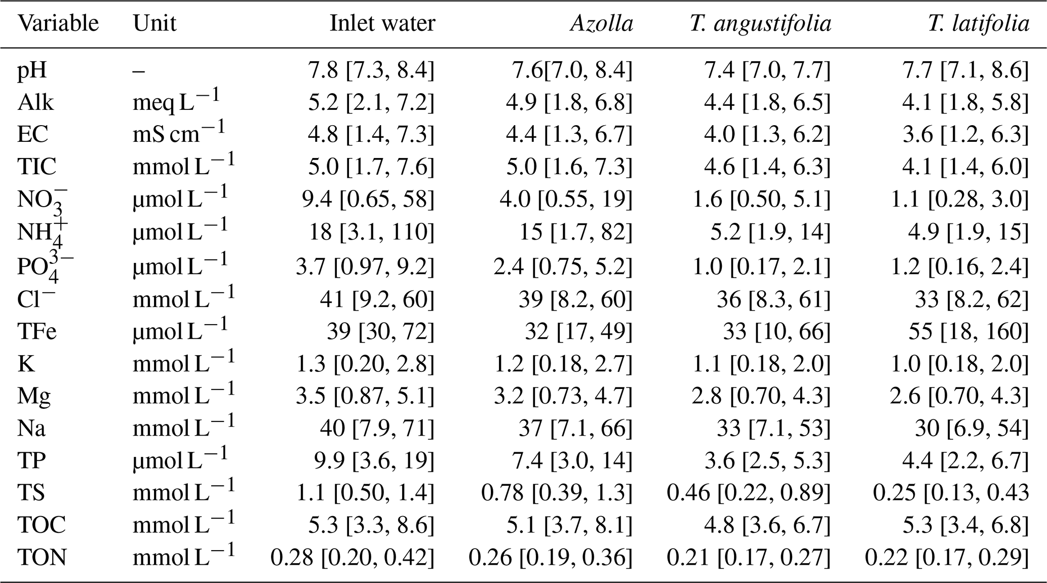
Table A2Pore water chemistry of pH, electrical conductivity (EC), total inorganic carbon (TIC), nitrate (NO), ammonium (NH), chloride (Cl), total iron (TFe), potassium (K), magnesium (Mg), sodium (Na), total phosphorus (TP), total sulfur (TS) , hydrogen sulfide (H2S), dissolved organic carbon (DOC), and dissolved organic nitrogen (DON) measured in the plots of the three different paludicrops. Between 8 and 10 measurements were taken over the whole season and averaged. The numbers in brackets denote the minimum and maximum measured.
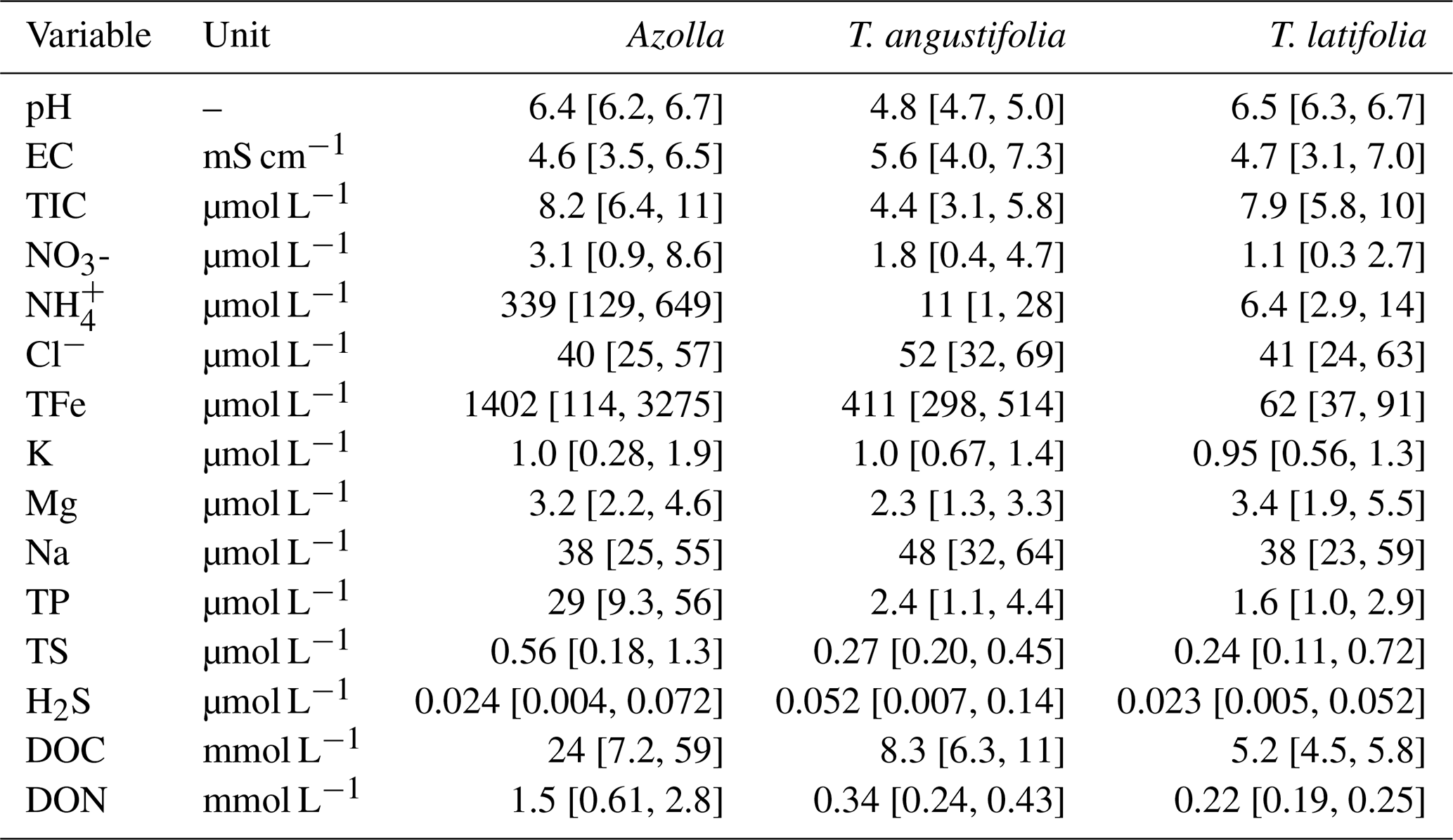
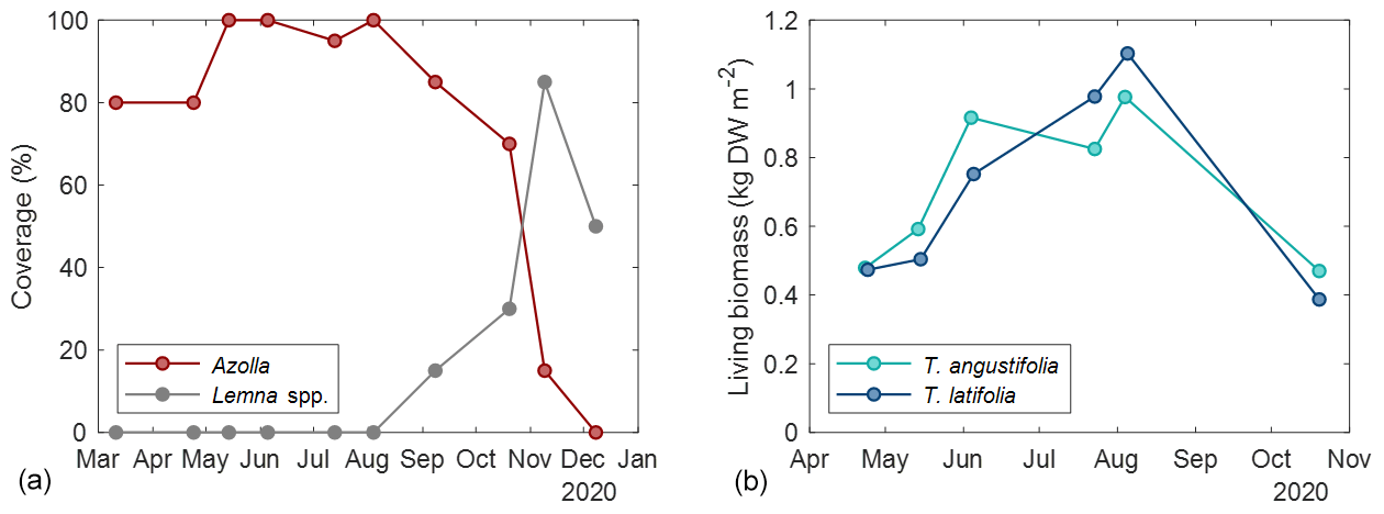
Figure B1Coverage of Azolla and Lemna spp. (a) and estimated living biomass based on stem count and stem height in the chamber plots for Typha (b) for the measuring year 2020.
All raw data can be provided by the corresponding author upon reasonable request.
BPvdR, MvdB, and AJPS designed the experiment. YvdV was responsible for the research setup at the reference site. TMG, RJEV, JvH, JB, and CJAvH carried out the experiment. TMG and RJEV did most of the data preparation. MvdB and TMG prepared the manuscript. MvdB did most of the writing, followed by TMG and RJEV. All other authors contributed to editing the manuscript.
The contact author has declared that none of the authors has any competing interests.
Publisher’s note: Copernicus Publications remains neutral with regard to jurisdictional claims made in the text, published maps, institutional affiliations, or any other geographical representation in this paper. While Copernicus Publications makes every effort to include appropriate place names, the final responsibility lies with the authors.
The measurements at the paludiculture site were part of the Peat Innovation Program initiated by the Association for Agricultural Nature and Landscape Management; Water, Land and Dijken (WLD); and the landscape conservation organization Landschap Noord-Holland (LNH). The measurements on the reference site were part of the Dutch national research program NOBV funded by the Dutch Ministry of Agriculture, Nature and Food Quality.
This research has been supported by the Peat Innovation Program initiated by the Association for Agricultural Nature and Landscape Management; Water, Land and Dijken (WLD); and the landscape conservation organization Landschap Noord-Holland (LNH), as well as the Dutch national research program NOBV funded by the Dutch Ministry of Agriculture, Nature and Food Quality. Renske J. E. Vroom and Bas P. van de Riet were supported by the NWO-TTW project AZOPRO (project no. 16294).
This paper was edited by Tyler Cyronak and reviewed by two anonymous referees.
Abdalla, M., Hastings, A., Truu, J., Espenberg, M., Mander, Ü., and Smith, P.: Emissions of methane from northern peatlands: a review of management impacts and implications for future management options, Ecol. Evol., 6, 7080–7102, https://doi.org/10.1002/ece3.2469, 2016.
Abel, S. and Kallweit, T.: Potential Paludiculture Plants of the Holarctic, Proceedings of the Greifswald Mire Centre 04/2022, ISSN 2627‐910X, 440 pp., 2022.
Aben, R. C. H., Barros, N., Van Donk, E., Frenken, T., Hilt, S., Kazanjian, G., Lamers, L. P. M., Peeters, E. T. H. M., Roelofs, J. G. M., De Senerpont Domis, L. N., Stephan, S., Velthuis, M., Van De Waal, D. B., Wik, M., Thornton, B. F., Wilkinson, J., DelSontro, T., and Kosten, S.: Cross continental increase in methane ebullition under climate change, Nat. Commun., 8, 1682, https://doi.org/10.1038/s41467-017-01535-y, 2017.
Anderson, C. M.: Cattail decline at Farmington Bay waterfowl management area, The Great Basin Naturalist, 24–34, 1977.
Arets, E. J. M. M., Lesschen, J. P., Lerink, B. J. W., Schelhaas, M., and Hendriks, C. M. J.: Information on LULUCF actions, The Netherlands Reporting in accordance to Article 10 of Decision No 529/2013/EU, Ministerie van LNV, https://edepot.wur.nl/538892 (last access: 21 July 2023), 2020.
Armstrong, J., Armstrong, W., Armstrong, I. B., and Pittaway, G. R.: Senescence, and phytotoxin, insect, fungal and mechanical damage: factors reducing convective gas-flows in Phragmites australis, Aquat. Bot., 54, 211–226, https://doi.org/10.1016/0304-3770(96)82384-9, 1996.
Attermeyer, K., Flury, S., Jayakumar, R., Fiener, P., Steger, K., Arya, V., Wilken, F., Van Geldern, R., and Premke, K.: Invasive floating macrophytes reduce greenhouse gas emissions from a small tropical lake, Sci. Rep., 6, 20424, https://doi.org/10.1038/srep20424, 2016.
Bansal, S., Johnson, O. F., Meier, J., and Zhu, X.: Vegetation Affects Timing and Location of Wetland Methane Emissions, J. Geophys. Res.-Biogeo., 125, e2020JG005777, https://doi.org/10.1029/2020JG005777, 2020.
Bastviken, D., Treat, C. C., Pangala, S. R., Gauci, V., Enrich-Prast, A., Karlson, M., Gålfalk, M., Romano, M. B., and Sawakuchi, H. O.: The importance of plants for methane emission at the ecosystem scale, Aquat. Bot., 184, 103596, https://doi.org/10.1016/j.aquabot.2022.103596, 2023.
Bendix, M., Tornbjerg, T., and Brix, H.: Internal gas transport in Typha latifolia L. and Typha angustifolia L., 1. Humidity-induced pressurization and convective throughflow, Aquat. Bot., 49, 75–89, https://doi.org/10.1016/0304-3770(94)90030-2, 1994.
Bharati, K., Mohanty, S. R., Singh, D. P., Rao, V. R., and Adhya, T. K.: Influence of incorporation or dual cropping of Azolla on methane emission from a flooded alluvial soil planted to rice in eastern India, Agr. Ecosyst. Environ., 79, 73–83, https://doi.org/10.1016/S0167-8809(99)00148-6, 2000.
Bocchi, S. and Malgioglio, A.: Azolla-Anabaena as a Biofertilizer for Rice Paddy Fields in the Po Valley, a Temperate Rice Area in Northern Italy, Int. J. Agron., 2010, 1–5, https://doi.org/10.1155/2010/152158, 2010.
Bodmer, P., Vroom, R. J. E., Stepina, T., Del Giorgio, P. A., and Kosten, S.: Methane dynamics in vegetated habitats in inland waters: quantification, regulation, and global significance, Front. Water, 5, 1332968, https://doi.org/10.3389/frwa.2023.1332968, 2024.
Bonn, A., Allott, T., Evans, M., Joosten, H., and Stoneman, R. (Eds.): Peatland Restoration and Ecosystem Services: Science, Policy and Practice, 1st Edn., Cambridge University Press, https://doi.org/10.1017/CBO9781139177788, 2016.
Boonman, J., Hefting, M. M., van Huissteden, C. J. A., van den Berg, M., Van Huissteden, J. (Ko), Erkens, G., Melman, R., and van der Velde, Y.: Cutting peatland CO2 emissions with water management practices, Biogeosciences, 19, 5707–5727, https://doi.org/10.5194/bg-19-5707-2022, 2022.
Boström, B., Andersen, J. M., Fleischer, S., and Jansson, M.: Exchange of Phosphorus Across the Sediment-Water Interface, in: Phosphorus in Freshwater Ecosystems, edited by: Persson, G. and Jansson, M., Springer Netherlands, Dordrecht, 229–244, https://doi.org/10.1007/978-94-009-3109-1_14, 1988.
Brouwer, P., Nierop, K. G. J., Huijgen, W. J. J., and Schluepmann, H.: Aquatic weeds as novel protein sources: Alkaline extraction of tannin-rich Azolla, Biotechnol. Rep., 24, e00368, https://doi.org/10.1016/j.btre.2019.e00368, 2019.
Buzacott, A. J. V., van den Berg, M., Kruijt, B., Pijlman, J., Fritz, C., Wintjen, P., and van der Velde, Y.: A Bayesian Inference Approach to Determine Experimental Typha Latifolia Paludiculture Greenhouse Gas Exchange Measured with Eddy Covariance, https://doi.org/10.2139/ssrn.4676190, 2023.
Clements, D.: Typha latifolia (broadleaf cattail), CABI Compend., CABI Compendium, 54297, https://doi.org/10.1079/cabicompendium.54297, 2022.
De Jong, M., Van Hal, O., Pijlman, J., Van Eekeren, N., and Junginger, M.: Paludiculture as paludifuture on Dutch peatlands: An environmental and economic analysis of Typha cultivation and insulation production, Sci. Total Environ., 792, 148161, https://doi.org/10.1016/j.scitotenv.2021.148161, 2021.
Desrosiers, K., DelSontro, T., and Del Giorgio, P. A.: Disproportionate Contribution of Vegetated Habitats to the CH4 and CO2 Budgets of a Boreal Lake, Ecosystems, 25, 1522–1541, https://doi.org/10.1007/s10021-021-00730-9, 2022.
Falge, E., Baldocchi, D., Olson, R., Anthoni, P., Aubinet, M., Bernhofer, C., Burba, G., Ceulemans, R., Clement, R., Dolman, H., Granier, A., Gross, P., Grünwald, T., Hollinger, D., Jensen, N.-O., Katul, G., Keronen, P., Kowalski, A., Lai, C. T., Law, B. E., Meyers, T., Moncrieff, J., Moors, E., Munger, J. W., Pilegaard, K., Rannik, Ü., Rebmann, C., Suyker, A., Tenhunen, J., Tu, K., Verma, S., Vesala, T., Wilson, K., and Wofsy, S.: Gap filling strategies for defensible annual sums of net ecosystem exchange, Agr. Forest Meteorol., 107, 43–69, https://doi.org/10.1016/S0168-1923(00)00225-2, 2001.
Forni, C., Chen, J., Tancioni, L., and Grilli Caiola, M.: Evaluation of the fern Azolla for growth, nitrogen and phosphorus removal from wastewater, Water Res., 35, 1592–1598, https://doi.org/10.1016/S0043-1354(00)00396-1, 2001.
Franz, D., Koebsch, F., Larmanou, E., Augustin, J., and Sachs, T.: High net CO2 and CH4 release at a eutrophic shallow lake on a formerly drained fen, Biogeosciences, 13, 3051–3070, https://doi.org/10.5194/bg-13-3051-2016, 2016.
Geurts, J. and Fritz, C.: Paludiculture pilots and experiments with focus on cattail and reed in the Netherlands, Radboud University, Nijmegen, the Netherlands, 2018.
Gremmen, T., van de Riet, B., van den Berg, M., Vroom, R. J. E., Weideveld, S. T. J., Van Huissteden, J., Westendorp, P.-J., and Smolders, A. J. P.: Natte teelten en veeteelt bij een verhoogd (grond)waterpeil in de veenweiden: de effecten van vernattingsmaatregelen op biogeochemie and broeikasgasemissies, B-WARE, Nijmegen, the Netherlands, 2022.
Grünfeld, S. and Brix, H.: Methanogenesis and methane emissions: effects of water table, substrate type and presence of Phragmites australis, Aquat. Bot., 64, 63–75, https://doi.org/10.1016/S0304-3770(99)00010-8, 1999.
Günther, A., Barthelmes, A., Huth, V., Joosten, H., Jurasinski, G., Koebsch, F., and Couwenberg, J.: Prompt rewetting of drained peatlands reduces climate warming despite methane emissions, Nat. Commun., 11, 1644, https://doi.org/10.1038/s41467-020-15499-z, 2020.
Hahn, J., Köhler, S., Glatzel, S., and Jurasinski, G.: Methane Exchange in a Coastal Fen in the First Year after Flooding – A Systems Shift, PLOS ONE, 10, e0140657, https://doi.org/10.1371/journal.pone.0140657, 2015.
Hahn-Schöfl, M., Zak, D., Minke, M., Gelbrecht, J., Augustin, J., and Freibauer, A.: Organic sediment formed during inundation of a degraded fen grassland emits large fluxes of CH4 and CO2, Biogeosciences, 8, 1539–1550, https://doi.org/10.5194/bg-8-1539-2011, 2011.
Haldan, K., Köhn, N., Hornig, A., Wichmann, S., and Kreyling, J.: Typha for paludiculture – Suitable water table and nutrient conditions for potential biomass utilization explored in mesocosm gradient experiments, Ecol. Evol., 12, e9191, https://doi.org/10.1002/ece3.9191, 2022.
Harpenslager, S. F., Van Den Elzen, E., Kox, M. A. R., Smolders, A. J. P., Ettwig, K. F., and Lamers, L. P. M.: Rewetting former agricultural peatlands: Topsoil removal as a prerequisite to avoid strong nutrient and greenhouse gas emissions, Ecol. Eng., 84, 159–168, https://doi.org/10.1016/j.ecoleng.2015.08.002, 2015.
Hemes, K. S., Chamberlain, S. D., Eichelmann, E., Knox, S. H., and Baldocchi, D. D.: A Biogeochemical Compromise: The High Methane Cost of Sequestering Carbon in Restored Wetlands, Geophys. Res. Lett., 45, 6081–6091, https://doi.org/10.1029/2018GL077747, 2018.
Hendriks, D. M. D., Van Huissteden, J., and Dolman, A. J.: Multi-technique assessment of spatial and temporal variability of methane fluxes in a peat meadow, Agr. Forest Meteorol., 150, 757–774, https://doi.org/10.1016/j.agrformet.2009.06.017, 2010.
Hoogland, T., Van Den Akker, J. J. H., and Brus, D. J.: Modeling the subsidence of peat soils in the Dutch coastal area, Geoderma, 171–172, 92–97, https://doi.org/10.1016/j.geoderma.2011.02.013, 2012.
Humpenöder, F., Karstens, K., Lotze-Campen, H., Leifeld, J., Menichetti, L., Barthelmes, A., and Popp, A.: Peatland protection and restoration are key for climate change mitigation, Environ. Res. Lett., 15, 104093, https://doi.org/10.1088/1748-9326/abae2a, 2020.
Huth, V., Günther, A., Bartel, A., Hofer, B., Jacobs, O., Jantz, N., Meister, M., Rosinski, E., Urich, T., Weil, M., Zak, D., and Jurasinski, G.: Topsoil removal reduced in-situ methane emissions in a temperate rewetted bog grassland by a hundredfold, Sci. Total Environ., 721, 137763, https://doi.org/10.1016/j.scitotenv.2020.137763, 2020.
IPCC (Intergovernmental Panel On Climate Change): Climate Change 2021 – The Physical Science Basis: Working Group I Contribution to the Sixth Assessment Report of the Intergovernmental Panel on Climate Change, 1st Edn., Cambridge University Press, https://doi.org/10.1017/9781009157896, 2021.
Irvin, J., Zhou, S., McNicol, G., Lu, F., Liu, V., Fluet-Chouinard, E., Ouyang, Z., Knox, S. H., Lucas-Moffat, A., Trotta, C., Papale, D., Vitale, D., Mammarella, I., Alekseychik, P., Aurela, M., Avati, A., Baldocchi, D., Bansal, S., Bohrer, G., Campbell, D. I., Chen, J., Chu, H., Dalmagro, H. J., Delwiche, K. B., Desai, A. R., Euskirchen, E., Feron, S., Goeckede, M., Heimann, M., Helbig, M., Helfter, C., Hemes, K. S., Hirano, T., Iwata, H., Jurasinski, G., Kalhori, A., Kondrich, A., Lai, D. Y., Lohila, A., Malhotra, A., Merbold, L., Mitra, B., Ng, A., Nilsson, M. B., Noormets, A., Peichl, M., Rey-Sanchez, A. C., Richardson, A. D., Runkle, B. R., Schäfer, K. V., Sonnentag, O., Stuart-Haëntjens, E., Sturtevant, C., Ueyama, M., Valach, A. C., Vargas, R., Vourlitis, G. L., Ward, E. J., Wong, G. X., Zona, D., Alberto, Ma. C. R., Billesbach, D. P., Celis, G., Dolman, H., Friborg, T., Fuchs, K., Gogo, S., Gondwe, M. J., Goodrich, J. P., Gottschalk, P., Hörtnagl, L., Jacotot, A., Koebsch, F., Kasak, K., Maier, R., Morin, T. H., Nemitz, E., Oechel, W. C., Oikawa, P. Y., Ono, K., Sachs, T., Sakabe, A., Schuur, E. A., Shortt, R., Sullivan, R. C., Szutu, D. J., Tuittila, E.-S., Varlagin, A., Verfaillie, J. G., Wille, C., Windham-Myers, L., Poulter, B., and Jackson, R. B.: Gap-filling eddy covariance methane fluxes: Comparison of machine learning model predictions and uncertainties at FLUXNET-CH4 wetlands, Agr. Forest Meteorol., 308/309, 108528, https://doi.org/10.1016/j.agrformet.2021.108528, 2021.
Joabsson, A. and Christensen, T. R.: Methane emissions from wetlands and their relationship with vascular plants: an Arctic example: METHANE EMISSION and VASCULAR PLANTS, Glob. Change Biol., 7, 919–932, https://doi.org/10.1046/j.1354-1013.2001.00044.x, 2001.
Kankaala, P., Mäkelä, S., Bergström, I., Huitu, E., Käki, T., Ojala, A., Rantakari, M., Kortelainen, P., and Arvola, L.: Midsummer spatial variation in methane efflux from stands of littoral vegetation in a boreal meso-eutrophic lake, Freshw. Biol., 48, 1617–1629, https://doi.org/10.1046/j.1365-2427.2003.01113.x, 2003.
Kimani, S. M., Cheng, W., Kanno, T., Nguyen-Sy, T., Abe, R., Oo, A. Z., Tawaraya, K., and Sudo, S.: Azolla cover significantly decreased CH4 but not N2O emissions from flooding rice paddy to atmosphere, Soil Sci. Plant Nutr., 64, 68–76, https://doi.org/10.1080/00380768.2017.1399775, 2018.
Kosten, S., Piñeiro, M., De Goede, E., De Klein, J., Lamers, L. P. M., and Ettwig, K.: Fate of methane in aquatic systems dominated by free-floating plants, Water Res., 104, 200–207, https://doi.org/10.1016/j.watres.2016.07.054, 2016.
Kroon, P. S., Schrier-Uijl, A. P., Hensen, A., Veenendaal, E. M., and Jonker, H. J. J.: Annual balances of CH4 and N2O from a managed fen meadow using eddy covariance flux measurements, Eur. J. Soil Sci., 61, 773–784, https://doi.org/10.1111/j.1365-2389.2010.01273.x, 2010.
Leifeld, J. and Menichetti, L.: The underappreciated potential of peatlands in global climate change mitigation strategies, Nat. Commun., 9, 1071, https://doi.org/10.1038/s41467-018-03406-6, 2018.
Li, F.-W., Brouwer, P., Carretero-Paulet, L., Cheng, S., de Vries, J., Delaux, P.-M., Eily, A., Koppers, N., Kuo, L.-Y., Li, Z., Simenc, M., Small, I., Wafula, E., Angarita, S., Barker, M. S., Bräutigam, A., dePamphilis, C., Gould, S., Hosmani, P. S., Huang, Y.-M., Huettel, B., Kato, Y., Liu, X., Maere, S., McDowell, R., Mueller, L. A., Nierop, K. G. J., Rensing, S. A., Robison, T., Rothfels, C. J., Sigel, E. M., Song, Y., Timilsena, P. R., Van de Peer, Y., Wang, H., Wilhelmsson, P. K. I., Wolf, P. G., Xu, X., Der, J. P., Schluepmann, H., Wong, G. K.-S., and Pryer, K. M.: Fern genomes elucidate land plant evolution and cyanobacterial symbioses, Nat. Plants, 4, 460–472, https://doi.org/10.1038/s41477-018-0188-8, 2018.
Liang, C. and Noble, A.: Chap. 11: N2O Emissions from Managed Soils, and CO2 Emissions from Lime and Urea Application, in: 2019 Refinement to the 2006 IPCC Guidelines for National Greenhouse Gas Inventories, 2019.
Liu, J., Xu, H., Jiang, Y., Zhang, K., Hu, Y., and Zeng, Z.: Methane Emissions and Microbial Communities as Influenced by Dual Cropping of Azolla along with Early Rice, Sci. Rep., 7, 40635, https://doi.org/10.1038/srep40635, 2017.
Lloyd, J. and Taylor, J. A.: On the Temperature Dependence of Soil Respiration, Funct. Ecol., 8, 315–323, https://doi.org/10.2307/2389824, 1994.
Lorenzen, B., Brix, H., Mendelssohn, I. A., McKee, K. L., and Miao, S. L.: Growth, biomass allocation and nutrient use efficiency in Cladium jamaicense and Typha domingensis as affected by phosphorus and oxygen availability, Aquat. Bot., 70, 117–133, https://doi.org/10.1016/S0304-3770(01)00155-3, 2001.
Maltais-Landry, G., Maranger, R., Brisson, J., and Chazarenc, F.: Greenhouse gas production and efficiency of planted and artificially aerated constructed wetlands, Environ. Pollut., 157, 748–754, https://doi.org/10.1016/j.envpol.2008.11.019, 2009.
Martens, M., Karlsson, N. P. E., Ehde, P. M., Mattsson, M., and Weisner, S. E. B.: The greenhouse gas emission effects of rewetting drained peatlands and growing wetland plants for biogas fuel production, J. Environ. Manag., 277, 111391, https://doi.org/10.1016/j.jenvman.2020.111391, 2021.
Matsui Inoue, T. and Tsuchiya, T.: Interspecific differences in radial oxygen loss from the roots of three Typha species, Limnology, 9, 207–211, https://doi.org/10.1007/s10201-008-0253-5, 2008.
McMillan, C.: Salt tolerance within a Typha population, Am. J. Bot., 46, 521–526, https://doi.org/10.1002/j.1537-2197.1959.tb07044.x, 1959.
Minick, K. J., Mitra, B., Noormets, A., and King, J. S.: Saltwater reduces potential CO2 and CH4 production in peat soils from a coastal freshwater forested wetland, Biogeosciences, 16, 4671–4686, https://doi.org/10.5194/bg-16-4671-2019, 2019.
Minke, M., Augustin, J., Burlo, A., Yarmashuk, T., Chuvashova, H., Thiele, A., Freibauer, A., Tikhonov, V., and Hoffmann, M.: Water level, vegetation composition, and plant productivity explain greenhouse gas fluxes in temperate cutover fens after inundation, Biogeosciences, 13, 3945–3970, https://doi.org/10.5194/bg-13-3945-2016, 2016.
Miranda, A. F., Biswas, B., Ramkumar, N., Singh, R., Kumar, J., James, A., Roddick, F., Lal, B., Subudhi, S., Bhaskar, T., and Mouradov, A.: Aquatic plant Azolla as the universal feedstock for biofuel production, Biotechnol. Biofuels, 9, 221, https://doi.org/10.1186/s13068-016-0628-5, 2016.
Murphy, K.: Typha angustifolia (lesser bulrush), CABI Compendium, https://doi.org/10.1079/cabicompendium.54294, 2022.
Pazourek, J.: The volumes of anatomical components in leaves of Typha angustifolia L. and Typha latifolia L., Biol. Plant., 19, 129–135, 1977.
Peters, G. A. and Meeks, J. C.: The Azolla-Anabaena symbiosis: Basic biology, Annu. Rev. Plant Physiol. Plant Mol. BioI., 40, 193–210, 1989.
Pieterse, A. H., De Lange, L., and Van Vliet, J. P.: A comparative study of azolla in the Netherlands, Acta Bot. Neerl., 26, 433–449, https://doi.org/10.1111/j.1438-8677.1977.tb01137.x, 1977.
Pijlman, J., Guerts, J., Vroom, R., Bestman, M., Fritz, C., and van Eekeren, N.: The effects of harvest date and frequency on the yield, nutritional value and mineral content of the paludiculture crop cattail (Typha latifolia L.) in the first year after planting, Mires Peat, 25, 1–19, https://doi.org/10.19189/MaP.2017.OMB.325, 2019.
Pinero-Rodríguez, M. J., Fernández-Zamudio, R., Arribas, R., Gomez-Mestre, I., and Díaz-Paniagua, C.: The invasive aquatic fern Azolla filiculoides negatively impacts water quality, aquatic vegetation and amphibian larvae in Mediterranean environments, Biol. Invasions, 23, 755–769, https://doi.org/10.1007/s10530-020-02402-6, 2021.
Quadra, G. R., Boonman, C. C. F., Vroom, R. J. E., Temmink, R. J. M., Smolders, A. J. P., Geurts, J. J. M., Aben, R. C. H., Weideveld, S. T. J., and Fritz, C.: Removing 10 cm of degraded peat mitigates unwanted effects of peatland rewetting: a mesocosm study, Biogeochemistry, 163, 65–84, https://doi.org/10.1007/s10533-022-01007-6, 2023.
Rey-Sanchez, A. C., Morin, T. H., Stefanik, K. C., Wrighton, K., and Bohrer, G.: Determining total emissions and environmental drivers of methane flux in a Lake Erie estuarine marsh, Ecol. Eng., 114, 7–15, https://doi.org/10.1016/j.ecoleng.2017.06.042, 2018.
Sebacher, D. I., Harriss, R. C., and Bartlett, K. B.: Methane Emissions to the Atmosphere Through Aquatic Plants, J. Environ. Qual., 14, 40–46, https://doi.org/10.2134/jeq1985.00472425001400010008x, 1985.
Sheppard, A., Shaw, R., and Sforza, R.: Top 20 environmental weeds for classical biological control in Europe: a review of opportunities, regulations and other barriers to adoption, Weed Res, 46, 93–117, https://doi.org/10.1111/j.1365-3180.2006.00497.x, 2006.
Sinicrope, T. L., Hine, P. G., Warren, R. S., and Niering, W. A.: Restoration of an Impounded Salt Marsh in New England, Estuaries, 13, 25–30, https://doi.org/10.2307/1351429, 1990.
Strachan, I. B., Nugent, K. A., Crombie, S., and Bonneville, M.-C.: Carbon dioxide and methane exchange at a cool-temperate freshwater marsh, Environ. Res. Lett., 10, 065006, https://doi.org/10.1088/1748-9326/10/6/065006, 2015.
Temmink, R. J. M., Harpenslager, S. F., Smolders, A. J. P., Van Dijk, G., Peters, R. C. J. H., Lamers, L. P. M., and Van Kempen, M. M. L.: Azolla along a phosphorus gradient: biphasic growth response linked to diazotroph traits and phosphorus-induced iron chlorosis, Sci. Rep., 8, 4451, https://doi.org/10.1038/s41598-018-22760-5, 2018.
Tiemeyer, B., Albiac Borraz, E., Augustin, J., Bechtold, M., Beetz, S., Beyer, C., Drösler, M., Ebli, M., Eickenscheidt, T., Fiedler, S., Förster, C., Freibauer, A., Giebels, M., Glatzel, S., Heinichen, J., Hoffmann, M., Höper, H., Jurasinski, G., Leiber-Sauheitl, K., Peichl-Brak, M., Roßkopf, N., Sommer, M., and Zeitz, J.: High emissions of greenhouse gases from grasslands on peat and other organic soils, Glob. Change Biol., 22, 4134–4149, https://doi.org/10.1111/gcb.13303, 2016.
Turetsky, M. R., Kotowska, A., Bubier, J., Dise, N. B., Crill, P., Hornibrook, E. R. C., Minkkinen, K., Moore, T. R., Myers-Smith, I. H., Nykänen, H., Olefeldt, D., Rinne, J., Saarnio, S., Shurpali, N., Tuittila, E., Waddington, J. M., White, J. R., Wickland, K. P., and Wilmking, M.: A synthesis of methane emissions from 71 northern, temperate, and subtropical wetlands, Glob. Change Biol., 20, 2183–2197, https://doi.org/10.1111/gcb.12580, 2014.
Van den Berg, M., van den Elzen, E., Ingwersen, J., Kosten, S., Lamers, L. P. M., and Streck, T.: Contribution of plant-induced pressurized flow to CH4 emission from a Phragmites fen, Sci. Rep., 10, 12304, https://doi.org/10.1038/s41598-020-69034-7, 2020.
Van den Born, G. J., Kragt, F., Henkens, D., Rijken, van Bemmel, B., and van der Sluis, S.: Dalende bodems, stijgende kosten, Intergovernmental Panel on Climate Change, Den Haag, 2016.
Van der Gon, H. A. C. D. and Neue, H.-U.: Methane emission from a wetland rice field as affected by salinity, Plant Soil, 170, 307–313, https://doi.org/10.1007/BF00010483, 1995.
Van der Nat, F. W. A., Middelburg, J. J., van Meteren, D., and Wielemakers, A.: Diel methane emission patterns from Scirpus lacustris and Phragmites australis, Biogeochemistry, 41, 1–22, 1998.
Van Kempen, M. M.: Azolla on top of the world: an ecophysiological study of floating fairy moss and its potential role in ecosystem services related to climate change, PhD Thesis, SI : [Sn], ISBN: 9789090279374, 2013.
Veenendaal, E. M., Kolle, O., Leffelaar, P. A., Schrier-Uijl, A. P., Van Huissteden, J., Van Walsem, J., Möller, F., and Berendse, F.: CO2 exchange and carbon balance in two grassland sites on eutrophic drained peat soils, Biogeosciences, 4, 1027–1040, https://doi.org/10.5194/bg-4-1027-2007, 2007.
Vroom, R. J. E., Xie, F., Geurts, J. J. M., Chojnowska, A., Smolders, A. J. P., Lamers, L. P. M., and Fritz, C.: Typha latifolia paludiculture effectively improves water quality and reduces greenhouse gas emissions in rewetted peatlands, Ecol. Eng., 124, 88–98, https://doi.org/10.1016/j.ecoleng.2018.09.008, 2018.
Vroom, R. J. E., van den Berg, M., Pangala, S. R., van der Scheer, O. E., and Sorrell, B. K.: Physiological processes affecting methane transport by wetland vegetation – A review, Aquat. Bot., 182, 103547, https://doi.org/10.1016/j.aquabot.2022.103547, 2022.
Vroom, R. J. E., Gremmen, T., van Huissteden, J., Smolders, A. J. P., van de Riet, B., Kosten, S., Fritz, C., and van den Berg, M.: Chimneys and blankets: species-dependent methane emissions in a rewetted Dutch peatland, Mires Peat, in review, 2024.
Wagner, G. M.: Azolla: A review of its biology and utilization, Bot. Rev., 63, 1–26, https://doi.org/10.1007/BF02857915, 1997.
Weier, K. L., Doran, J. W., Power, J. F., and Walters, D. T.: Denitrification and the Dinitrogen/Nitrous Oxide Ratio as Affected by Soil Water, Available Carbon, and Nitrate, Soil Sci. Soc. Am. J., 57, 66–72, https://doi.org/10.2136/sssaj1993.03615995005700010013x, 1993.
White, S. D. and Ganf, G. G.: Flow characteristics and internal pressure profiles in leaves of the Typha domingensis, Aquat. Bot., 67, 263–273, https://doi.org/10.1016/S0304-3770(00)00100-5, 2000.
Wichtmann, W. and Joosten, H.: Paludiculture: Peat formation and renewable resources from rewetted peatlands, IMCG Newsletter, 3, 24–28, 2007.
Xu, H., Zhu, B., Liu, J., Li, D., Yang, Y., Zhang, K., Jiang, Y., Hu, Y., and Zeng, Z.: Azolla planting reduces methane emission and nitrogen fertilizer application in double rice cropping system in southern China, Agron. Sustain. Dev., 37, 29, https://doi.org/10.1007/s13593-017-0440-z, 2017.
Yavitt, J. B. and Knapp, A. K.: Aspects of methane flow from sediment through emergent cattail (Typha latifolia) plants, New Phytol., 139, 495–503, https://doi.org/10.1046/j.1469-8137.1998.00210.x, 1998.
Zhang, M., Xiao, Q., Zhang, Z., Gao, Y., Zhao, J., Pu, Y., Wang, W., Xiao, W., Liu, S., and Lee, X.: Methane flux dynamics in a submerged aquatic vegetation zone in a subtropical lake, Sci. Total Environ., 672, 400–409, https://doi.org/10.1016/j.scitotenv.2019.03.466, 2019.