the Creative Commons Attribution 4.0 License.
the Creative Commons Attribution 4.0 License.
 | 22 Aug 2024
High-frequency continuous measurements reveal strong diel and seasonal cycling of pCO2 and CO2 flux in a mesohaline reach of the Chesapeake Bay
Jim R. Muirhead
Amanda C. Reynolds
Mark S. Minton
Karl J. Klug
We estimated hourly air–water gas transfer velocities (k600) for carbon dioxide in the Rhode River, a mesohaline sub-estuary of the Chesapeake Bay. Gas transfer velocities were calculated from estuary-specific parameterizations developed explicitly for shallow microtidal estuaries in the mid-Atlantic region of the United States, using standardized wind speed measurements. Combining the gas transfer velocity with continuous measurements of pCO2 in the water and in the overlying atmosphere, we determined the direction and magnitude of CO2 flux at hourly intervals across a 3-year record (1 July 2018 to 1 July 2021). Continuous year-round measurements enabled us to document strong seasonal cycling, whereby the Rhode River is primarily autotrophic during cold-water months (December–May) and largely net heterotrophic in warm-water months (June–November). Although there is inter-annual variability in CO2 flux in the Rhode River, the annual mean condition is near carbon neutral. Measurement at high temporal resolution across multiple years revealed that CO2 flux and apparent trophic status can reverse during a single 24 h period. pCO2 and CO2 flux are mediated by temperature effects on biological activity and are inverse to temperature-dependent physical solubility of CO2 in water. Biological/biogeochemical carbon fixation and mineralization are rapid and extensive, so sufficient sampling frequency is crucial to capture unbiased extremes and central tendencies of these estuarine ecosystems.
- Article
(2600 KB) - Full-text XML
-
Supplement
(2961 KB) - BibTeX
- EndNote


Understanding the air–sea exchange of gases and establishing methodologies for accurate measurements has been a decades-long focus of atmospheric scientists, oceanographers, and biogeochemists seeking to understand interactions between oceans and the atmosphere and how these interactions contribute to the global carbon cycle (Broecker et al., 1979; Wanninkhof, 1992; Wanninkhof et al., 2013). Coastal oceans and estuaries are ecosystems of interest for understanding the complex nature and contribution of the land–sea interface to lateral mass transport of carbon (Abril and Borges, 2005; Cai and Wang, 1998; Frankignoulle et al., 1998; Song et al., 2023) but also with respect to the role these ecosystems play as both atmospheric CO2 sources and sinks (Abril and Borges, 2005; Chen et al., 2020; Dai et al., 2022; Jiang et al., 2008). The exchange of carbon dioxide, methane, and other greenhouse gases (GHGs) between Earth's atmosphere and inland waters, estuaries, and coastal oceans are well-documented but not fully quantified (Abril and Borges, 2005; Cai, 2011; Laruelle et al., 2017; Raymond and Cole, 2001; Raymond et al., 2013; Van Dam et al., 2019). CO2 evasion from estuaries alone has been estimated at 15 %–17 % of the total CO2 input from oceans to the atmosphere (Chen et al., 2020; Laruelle et al., 2017), indicating the regional and global significance of estuaries (Bauer et al., 2013; Frankignoulle et al., 1998; Jiang et al., 2008). Yet, there is still great uncertainty surrounding the true net contributions of coastal oceans, estuaries, and inland water bodies to the atmospheric loading of GHGs (Borges, 2005; Chen et al., 2020; Herrmann et al., 2020; Joesoef et al., 2015; Laruelle et al., 2017; Raymond et al., 2013; Van Dam et al., 2019).
To better understand the effects of estuaries on atmospheric GHG exchange and accumulation, it is imperative that we understand their capacity and function as carbon sources and sinks and ultimately how estuaries factor into the planet's overall global carbon budget (Herrmann et al., 2020; Laruelle et al., 2017; Van Dam et al., 2019). Many attempts to characterize CO2 flux in estuaries and nearshore oceans (Chen et al., 2013; Herrmann et al., 2020; Rosentreter et al., 2021) have relied on direct measurements using floating domes, tracer gases or, more recently, eddy covariance methods (Laruelle et al., 2017; Van Dam et al., 2019). Because flux measurements are time intensive, they tend to be temporally and spatially limited (Herrmann et al., 2020; Klaus and Vachon, 2020). Using direct flux measurements to derive accurate gas transfer velocity constants (k, the velocity of gas crossing the air–water boundary) enables models to be parameterized to estimate k and compute gas flux. Thus, correlative models that incorporate simultaneous environmental measurements such as wind and/or water velocity, factors that affect turbulence at the air–water interface and promote gas exchange, have aided in the widespread accumulation of gas flux estimates (Raymond and Cole, 2001; Van Dam et al., 2019; Wanninkhof, 2014). Gas transfer velocity constant models vary according to the habitat/system being observed and chemical, physical, and biological factors present in each (e.g., lakes, rivers/streams, estuaries, and oceans; Herrmann et al., 2020; Ho et al., 2016; Raymond and Cole, 2001; Van Dam et al., 2019; Wanninkhof, 1992). To reduce uncertainty in computed gas fluxes, it is critical that the appropriate k models are matched to a targeted ecosystem.
Coastal oceans and estuaries are exceptionally complex, frequently characterized by their relative shallowness and by how their freshwater inputs (riverine, surface, and groundwater) mix with saltwater (Chen et al., 2020). High nutrient and pollutant loading due to urbanization and eutrophication by humans also have important effects on estuaries and coastal oceans (Freeman et al., 2019). High spatial and temporal variability are hallmarks of estuaries.
Here we present a 3-year data set that combines high-frequency (1 min interval) measurements of dissolved and atmospheric CO2 with co-located and continuous measurements of salinity, water temperature, tidal cycling, and wind velocity, recorded at the Smithsonian Environmental Research Center (SERC) dock in the Rhode River, Maryland. To estimate hourly, daily, seasonal, and annual CO2 flux rates, we applied a CO2 gas velocity constant model developed by Van Dam et al. (2019) for the New River, North Carolina. This model is expressly designed for application to shallow well-mixed microtidal estuaries located on the mid-Atlantic coast of the United States.
2.1 Study location
The Rhode River is a tributary and sub-estuary of the Chesapeake Bay, a drowned river valley coastal-plain estuary (Fig. 1). The Rhode River has been studied extensively by SERC staff and colleagues for over 4 decades: nutrient chemistry (Jordan and Correll, 1991; Jordan et al., 1991), phytoplankton ecology (Gallegos et al., 2010), color dissolved organic matter distribution (Tzortziou et al., 2008, 2011), and more recently, modeling of dissolved organic carbon (DOC) input from freshwater and tidal marsh sources have all been researched (Clark et al., 2020). Located on the bay's northwestern shore (38°52′ N, 76°32′ W), the Rhode River is bounded at its head by Muddy Creek and at its mouth by the mainstem of the Chesapeake Bay. The Rhode River is a shallow (mean depth = 2 m, max depth = 4.1 m) mesohaline (0 to 18 ppt) well-mixed eutrophic tributary with a length of approximately 5 km; its surface area is approximately 5 km2, with a shoreline perimeter of 39 km (Breitburg et al., 2008; Clark et al., 2018). A 0.21 km2 tidal marsh (Kirkpatrick Marsh) fringes the estuary at the mouth of Muddy Creek (Fig. 1). Tides are semi-diurnal with a mean amplitude of approximately 30 cm, but water height can be strongly affected by wind and weather events. Muddy Creek is the main freshwater source of the Rhode River and has a maximum flow rate of 10.42 m3 s−1 and mean flow rate 0.18 m3 s−1 (mean flow = 15 552 m3 d−1; Clark et al., 2020, 2018; Jordan et al., 1986). The mean daily volume of freshwater inflow from Muddy Creek is approximately 0.5 % of the mean daily tidal exchange volume based on the Rhode River's area and mean tidal amplitude. In the absence of measurements of the pH or pCO2 of the freshwater entering the Rhode River from Muddy Creek or other lesser freshwater inputs to the estuary, we are unable to report these pCO2 or pH values. However, given the exceedingly small overall volume of freshwater input to the Rhode River from its surrounding watershed, it is not considered a river-dominated estuary so is not expected to be substantially influenced by the chemical characteristics of this input. This is not to say that there is no freshwater influence, only that such influences are likely quite local when mixing with far larger volumes of water from the Chesapeake Bay and therefore beyond the resolution of this study.
Although the Rhode River is a model ecosystem that has been studied intensively for several decades across many dimensions (Clark et al., 2018; Correll et al., 1992; Gallegos et al., 1992; Jordan et al., 1991; Rose et al., 2019), no work to date has expressly characterized the nature and dynamics of CO2 flux between the river and the atmosphere.
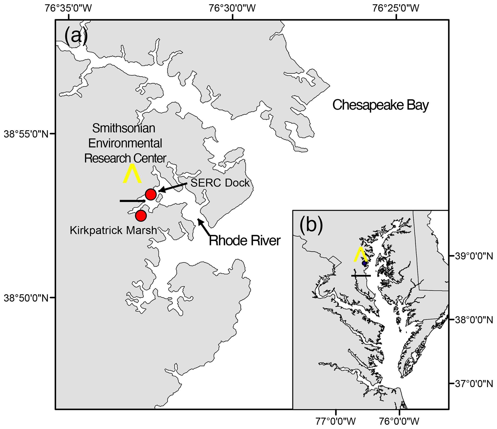
Figure 1Location of study site on the Rhode River, Edgewater, MD (a), as situated in the Chesapeake Bay (b). All pCO2 and related water quality values reported were measured from the SERC dock, which extends approximately 75 m from the shore into the Rhode River. Red circles indicate locations of the dock and a tidal creek that drains the Kirkpatrick salt marsh (marsh area is equal to 0.21 km2, 1 km up estuary from the dock).
2.2 In situ measurements, calculated parameters, and quantities
Continuous, automated environmental measurements were made in and above the Rhode River during a 3-year period between 1 July 2018 and 1 July 2021. The purpose of these measurements was to document fluctuations in aqueous pCO2 on a fine timescale, from which CO2 flux between the water and atmosphere could be calculated.
2.2.1 Aqueous CO2 (pCO2 water)
To measure the CO2 gradient () across the Rhode River surface waters and its overlying atmosphere, measurements of pCO2 were made with a nondispersive infrared (NDIR) detector. In the case of dissolved gas measurements, water was equilibrated continuously with a spherical falling film equilibrator (Miller et al., 2019). Water from 1 m below the water's surface was pumped and dispersed continuously over a 25.4 cm diameter sphere. The falling film created on the sphere generates a gas exchange surface, which forces CO2 in the equilibrator headspace into equilibrium with the water's CO2 content, i.e., mole fraction = xCO2 (µmol mol−1). Water exits the equilibrator via an airtight drain that prevents headspace contamination from surrounding atmospheric air. Headspace gas circulates continuously in a closed loop through the equilibrator, water trap, and gas dehumidifier; past the NDIR; and back into the equilibrator. Experimental observations concluded that spherical falling film equilibrators achieve 99 % equilibration of CO2 within 10–15 min, depending on whether step changes are from low to high or high to low; details of the operation and performance of the falling film equilibrator are described in Miller et al. (2019). Measurements were made at 1 min intervals at a pressure equal to the ambient barometric pressure.
Measured raw CO2 mole fractions (µmol mol−1) were converted to partial pressures (µatm) using Eq. (1). Minute-over-minute values were rounded down to the nearest hour and averaged to provide hourly means. The mole fractions were then evaluated with corresponding water temperature and salinity measurements following the methodology of Zeebe and Wolf-Gladrow (2001), where the saturation vapor pressure of water is calculated according to Weiss and Price (1980) to determine pCO2 water.
where pCO2 is the partial pressure of CO2 of water (µatm); xCO2 is the mole fraction of CO2 in water (µmol mol−1); p is total pressure, which is equal to 1 atm; and pH2O is the saturation vapor pressure of water (µatm).
2.2.2 Atmospheric CO2
Every 6 h, the sample gas stream was automatically diverted with programmed solenoid control valves from the equilibrator to an atmospheric port located approximately 5 m above the pier deck. During atmospheric sampling, 15 1 min interval measurements were made. To account for inaccuracies during the transition period from equilibrator to atmospheric sampling, the final eight measurements were averaged and the first seven were discarded. Similarly, the first 30 measurements following switchover from atmospheric port to equilibrator were discarded, to ensure that measurements were fully equilibrated with water. For these atmospheric measurements, the contribution of the vapor pressure of water to the total atmospheric pressure of the open-air environment was considered negligible (i.e., pH2O=0 and p=1), such that pCO2 atm=xCO2 atm. As such, any potential differences are expected to fall well within the measurement accuracy of the instrument (see below).
One advantage to using a shared NDIR sensor for aquatic and atmospheric samples is that any minor effects of instrument drift will be reflected in both data streams, as opposed to two sensors that drift independently of one another. Likewise, significant and sustained deviation from typical local atmospheric variability will be captured during atmospheric sampling and can signal the need for recalibration and assist with the quality assurance or quality control of corresponding data from both streams. A disadvantage of using a common sensor for both dissolved and atmospheric CO2 measurements is that it results in a mismatch in sampling frequency of the two. With this limitation in mind, we chose a higher sampling frequency for aquatic measurements to better describe the inherently higher variability in dissolved CO2 in water vs. that in the atmosphere (Fig. 2).
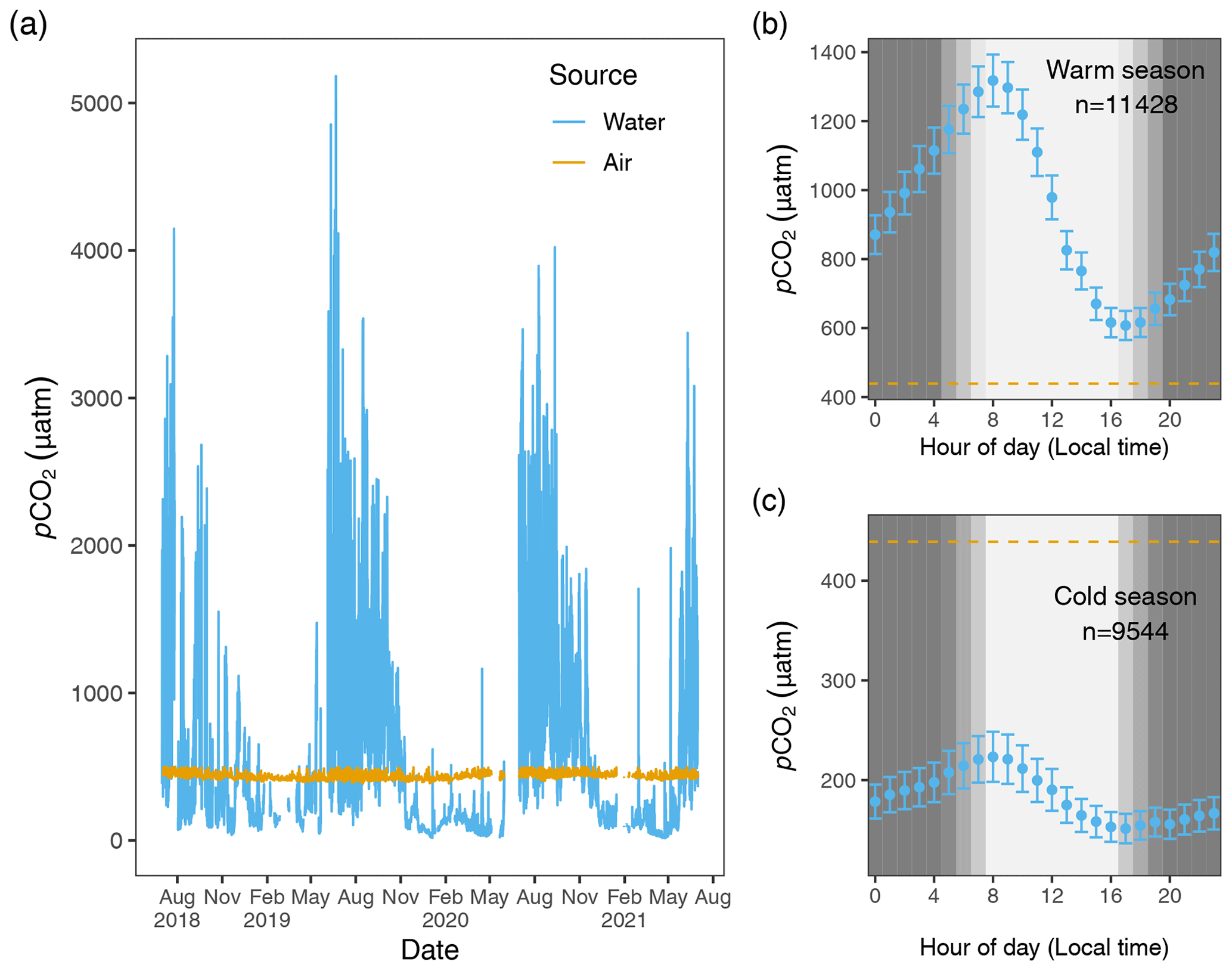
Figure 2Hourly pCO2 water (blue) and pCO2 air (goldenrod) values from 1 July 2018 to 1 July 2021 (a). The air–water CO2 gradient, , describes the directionality of gas diffusion. Negative ΔC values (pCO2 water values falling below the goldenrod demarcation) represent gas movement from air to water and vice versa. Panels (b) and (c) depict mean pCO2 water values (95 % CI) for each hour of the day for warm and cold seasons, with the dashed lines equal to the mean 3-year value of pCO2 air.
Given the 3-year time series and strong diel cycling of pCO2 water (and dissolved oxygen, DO; see Figs. S1 and S2 in the Supplement) in the Rhode River, we chose to aggregate aqueous minute-over-minute measurements to mean hourly averages. Owing to the relative lack of short-term variability in local atmospheric CO2 concentrations (Fig. 2), we used linear interpolation to impute atmospheric CO2 concentrations during the hours in between actual readings (6 h gaps between atmospheric measurements), which we assumed to be more realistic and reliable than last observation carried forward (LOCF) methods, where the last observation is repeated for all gaps until the next measurement is encountered, a method that has fallen out of favor, especially for environmental time series data (Lachin, 2016). To determine if any inadvertent bias was introduced by the linear interpolation procedure, summary statistics of actual atmospheric readings and actual readings plus imputed CO2 values were compared statistically. This approach enabled us to take advantage of >25 000 time points throughout the 3-year period of observation, providing hourly resolution. Mean pCO2 air=437 ± 20.0 µatm (Table 1), variability that falls well within manufacturer's specifications (see Sect. 2.2.4).
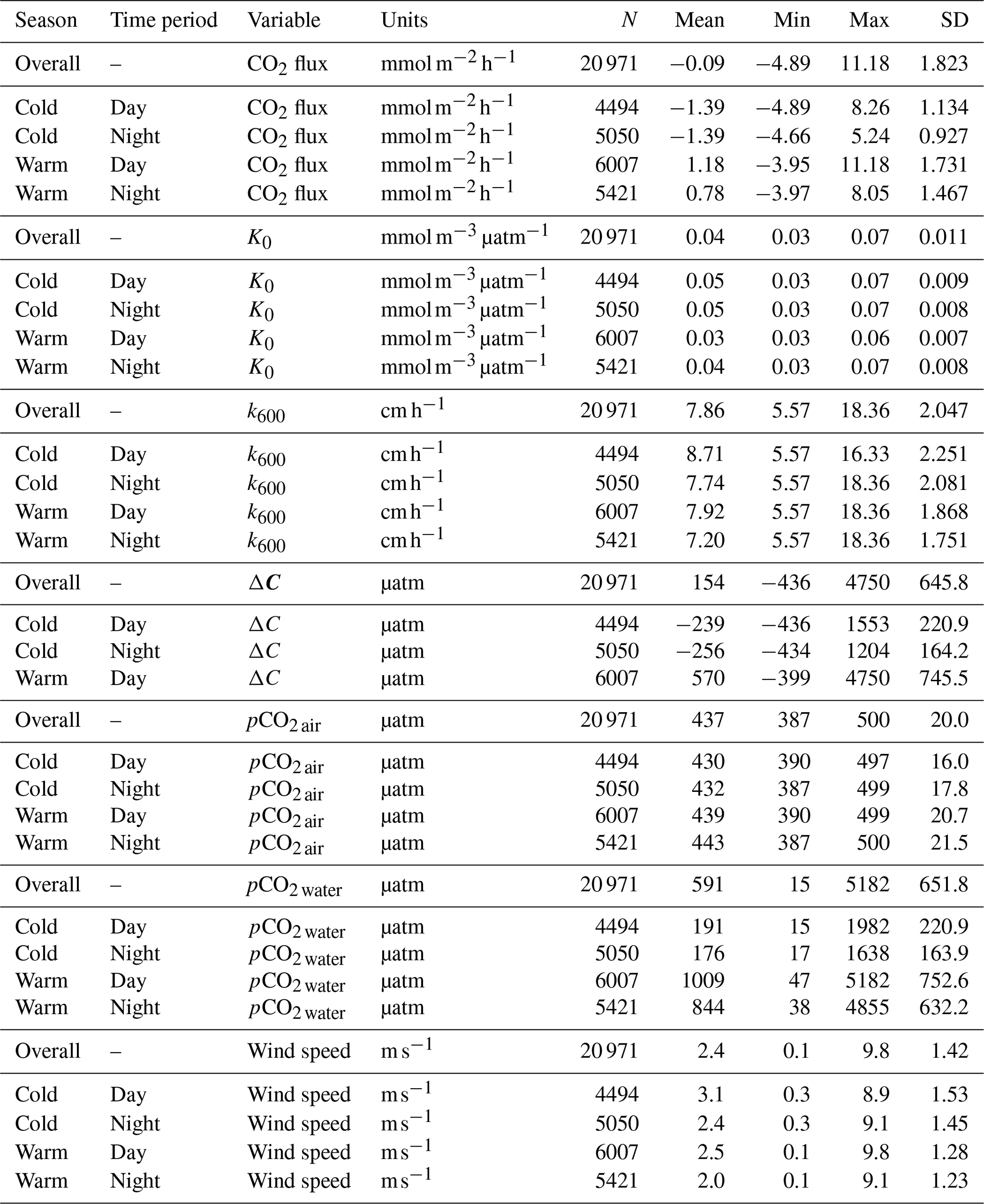
Table 1Descriptive statistics comparing the seasonality of pCO2, CO2 flux, and associated parameters in cold-water (December–May) and warm-water seasons (June–November).
2.2.3 CO2 gradient (ΔC)
ΔC was determined by subtraction, pCO2 water−pCO2 air, where positive ΔC values correspond to higher CO2 concentrations in the water, tending toward movement from water to air (outgassing or evasion, where Rhode River is a CO2 source), and negative values signal CO2 transport from air to water (dissolution, where Rhode River is a CO2 sink). Figure 2 shows pCO2 water and pCO2 air plotted on an hourly basis for the 3-year period beginning 1 July 2018 and ending 1 July 2021. Across this period, ΔC was predominantly negative during cold months and predominantly positive during warm months when pCO2 water tended to reach the highest values of the year, but ΔC sometimes reversed sign due to occasional extreme daytime photosynthetic drawdown of CO2 (Fig. 2).
2.2.4 Accuracy of CO2 measurements
Estimated accuracy of the spherical falling film equilibrator and NDIR sensor (Senseair K30, https://senseair.com/, last access: 15 December 2023) combination was experimentally determined in the lab and found to measure water equilibrated with known gas concentrations to within the ±1 % uncertainty limits of the of certified standard gas mixtures used, well within the published accuracy specification of the Senseair K30 (i.e., ±30 ppmv ± 3 % of instrument reading). Experimental analysis by Martin et al. (2017) report even higher accuracy when relative humidity and atmospheric pressure are controlled for. Details on performance of the spherical falling film equilibrator, such as accuracy, precision, and time constants, can be found in Miller et al. (2019). Although Senseair offers automated calibration via long-term comparisons to atmospheric readings, this feature was deactivated. The K30 NDIR was periodically validated using standard zero CO2 (nitrogen) and standard certified span gases at intervals of 1–2 months during the study period. Although the K30 was never observed to drift beyond its factory specifications, the sensor was occasionally re-calibrated in the lab, and measured values were accepted without adjustment.
CO2 measurements were downloaded to a database at approximately 2-week intervals during the observation period. Data were graphed and reviewed visually in combination with twice-weekly observations of equilibrator function recorded in an accompanying notebook. Anomalous data were flagged and excluded from data analysis (e.g., flooding or clogging events that interrupted proper equilibration.)
2.3 Co-located water quality and atmospheric measurements
This water quality station at the SERC dock is a long-term node of the Maryland Department of Natural Resources (DNR) “Eyes on the Bay” Chesapeake Bay tidal water monitoring program and has been operated by the SERC since 1986. Water quality and atmospheric data are maintained by the MarineGEO Upper Chesapeake Bay Observatory and can be accessed online (Benson et al., 2023). A YSI EXO2 sonde was positioned 1 m below the water's surface and in proximity (∼2.5 m distance) to the submerged water pump that fed the pCO2 equilibrator. Sonde measurements were made at 6 min intervals and aggregated to 1 h averages. The published accuracy specifications for the YSI sonde are as follows: temperature – ±0.01 °C (−5 to 35 °C), salinity – ±1 % of reading or 0.1 ppt (0–70 ppt), and dissolved oxygen – ±0.1 mg L−1 or 1 % of reading (0 to 20 mg L−1). Discrete measurements of temperature and salinity were made using a handheld YSI Professional Plus 2030 with Quattro Cable instrument with the following specifications: temperature – ±0.02 °C (−5 to 70 °C), salinity – ±1 % of reading or 0.1 ppt (0–70 ppt), and dissolved oxygen – ±0.2 mg L−1 or 2 % of reading (0 to 20 mg L−1). Equilibrator temperature was measured with a probe (EDS model OW-TEMP-B3-12xA) accurate to ±0.5 °C (−10 to 85 °C). Discrete measurements were routinely compared to the sonde to corroborate measurement agreement. Wind speed measurements were made using a sonic anemometer (Vaisala WXT-520 weather transmitter) mounted 7 m above the mean low-tide height of the water and located directly above the pCO2 equilibrator.
2.4 Data processing
Data included in this study span 1 July 2018 to 1 July 2021.
2.4.1 Gas-specific solubility
To determine the purely physical effects of temperature and salinity on CO2 solubility, gas-specific solubility values K0 () were calculated across the 3-year observation period using water temperature and salinity measurements in combination with pCO2 water values, according to Weiss and Price (1980), at 1 h intervals.
2.4.2 Gas transfer velocity estimation (k)
Given the similarities between the Rhode River and New River estuaries (e.g., shallow microtidal estuaries with slow water velocity and strong diel cycles in pCO2 and DO), we chose to parameterize gas transfer velocity k (cm h−1) standardized to the unitless Schmidt number 600 (k600) according to the estuary-specific k parameterization model developed by Van Dam et al. (2019). Van Dam et al. (2019) determined that k correlated with wind speed differently during daytime vs. nighttime hours (linear vs. parabolic relationships). Wind speed data were collected during the 3-year period from a sonic anemometer located on the SERC dock directly above the equilibration system and approximately 7 m above the water's surface at mean low-tide height. For the analysis, wind speeds were standardized for a height of 10 m following a power-law relationship, (Saucier, 2003). Following Van Dam et al., wind speed data were binned to 1.5 m s−1 intervals for day and night readings and raw values replaced by the mean wind speed for each bin. The median binned wind speed over the Rhode River was 2.2 m s−1 regardless of time of day or season. Recorded wind speeds never exceeded 10 m s−1 and were dominated by much lower values (Fig. S1). Unlike the New River Estuary, the Rhode River's wind speed profile does not differ much between day and night, nor across seasons. For this reason, we chose to use the most conservative k600 formulation from Van Dam et al. (2019) that combines day and night winds to estimate k600.
Wind speed was used to parameterize k600 as follows:
where U10 is the mean of binned wind speed at 10 m above the water's surface (m s−1).
2.4.3 CO2 flux
Using continuous, parallel 3-year records (1 July 2018 to 1 July 2021) of dissolved and atmospheric pCO2, water temperature, salinity, and wind speed (at standard 10 m height; U10), CO2 flux was derived according to the equation
where CO2 flux is the rate and direction of the CO2 mass moving between water and gas phases (), k600 is the gas transfer velocity (cm h−1) normalized to a common Schmidt number (Sc=600), K0 is gas-specific solubility for CO2 (), ΔC is the air–water concentration gradient (µatm), and Sc is the Schmidt number.
Note: CO2 flux calculations require conversion from traditional k600 units (cm h−1) to m h−1 and from ΔC units (µatm) to atm prior to calculation.
2.4.4 Day–night designation
To differentiate daytime from nighttime hours, we used the position of the measurements (latitude) in the Rhode River combined with the local date and time. This approach enabled us to uniformly designate various environmental measurements as happening during the day or night (R package LakeMetabolizer; Winslow et al., 2016).
2.4.5 Seasonality
We chose to break the year into two 6-month periods based on seasonal water temperature shifts, designating June–November as “warm-water months” when water temperatures averaged 23.2 ± 6.90 °C (mean ± 1 SD) and December–May as “cold-water months”, 10.9 ± 5.66 °C (Figs. S1 and S2).
2.4.6 Effect size
Owing to the large number of observations available for comparison in this study, the likelihood of finding statistically significant results is quite high. Whether such statistical results by themselves connote practical and informative differences can be difficult to discern. Effect sizes (omega-squared, ω2) were calculated according to two-factor analyses of variance (ANOVAs) where independent variables were investigated by season (cold-water vs. warm-water season) and day–night period and the interaction of season and day–night. The independent variables compared were K0, CO2 flux, ΔpCO2, k600, pCO2 air, pCO2 water, and wind speed. To account for temporal autocorrelation and lack of independence of observations that are typical of environmental time series data, we corrected for overinflation in the residual mean square used in the effect size calculations by removing the autocorrelation present within residuals, leaving the white-noise component as the unbiased estimate of residual variability (Cochrane–Orcutt procedure, R package orcutt; Spada et al., 2018).
3.1 Daily and seasonal cycling of pCO2
Hourly averaged measurements of pCO2 water in the Rhode River across 3 years revealed strong diel and seasonal cycling (Fig. 2). Mean and maximum pCO2 water were significantly higher in warm-water vs. cold-water months (Table 1). During warm-water months (June–November), daily oscillations of pCO2 frequently transit from far above to below ambient atmospheric conditions over the course of the day, only to reverse direction (from low to high) during the nighttime hours (Fig. 2). During the summer, pCO2 water levels sometimes shifted by as much as 4500 µatm in both directions during a single 24 h period (Fig. 2). This pattern is consistent with biologically driven cycling whereby very high early morning pCO2 water conditions are depleted by net photosynthetic activity (inorganic carbon fixation) over the course of the day, but high pCO2 water is restored by respiration in the benthos and water column at night (Song et al., 2023). Comparing dissolved oxygen (DO) over the same period, similar harmonic cycling is observed, but maxima and minima of pCO2 and DO were inversely related (Fig. S1), hallmarks of a production/respiration-driven system (Herrmann et al., 2020; Van Dam et al., 2019).
On the seasonal timescale, pCO2 was consistently lowest and DO highest during cold-water months of the year (December–May; Fig. S1). Importantly, for both gases the temporal variability (diel cycling; Fig. S2) was most constrained during cold-water months across years, strongly suggesting that carbon fixation exceeds respiration for prolonged periods (weeks to months). In contrast, during warm-water months (June–November), photosynthesis/carbon fixation and respiration are more evenly balanced, compensating for one another over 24 h periods (i.e., respiration > productivity at night and productivity > respiration during daylight hours; Fig. 2).
3.2 Air–water concentration gradient = ΔC (µatm)
When hourly pCO2 water and pCO2 air values (composed of 4 hourly measurements and 20 interpolated values per day) were plotted across the 3 years of observation, the diel and seasonal cycles of pCO2 water are evident. As expected, atmospheric concentrations of CO2 remained relatively constant compared with aqueous loads. When the mean raw pCO2 air measurements (mean=435.1, 95 % CI [434.4,435.7]) were compared with raw pCO2 air measurements plus imputed estimates (mean=435.4, 95 % CI [435.2,435.7]) no statistical difference was observed, indicating that no substantial bias was introduced by linear interpolation of atmospheric measurements.
Although nearshore atmospheric CO2 concentrations are expected to vary more than those in an isolated well-mixed atmosphere (e.g., at the Mauna Loa Observatory), annual mean values were consistent and within the published uncertainty of the K30 NDIR sensor when compared with global measurements conducted at Mauna Loa (Thoning et al., 2023). Local perturbations (e.g., effects of terrestrial photosynthetic drawdown when wind is absent) were apparent in measurements (Fig. 2), but there were no instances when the measured local atmospheric values were suspiciously high or low for days on end, as compared to expected global mean atmospheric values for the time period (i.e., 408–416 ppmv; https://www.co2.earth/annual-co2, last access: 15 December 2023, Thoning et al., 2023). This lack of sustained anomalous deviation served as additional confirmation that the K30 was functioning properly and had not drifted outside its calibration range. Importantly, given the extreme diel cycling and seasonal variability in the Rhode River's pCO2 water, the absolute accuracy necessary for determining year-over-year changes in atmospheric or ocean pCO2 is not a requirement for these CO2 flux calculations that rely on relative differences between water and atmospheric measurements.
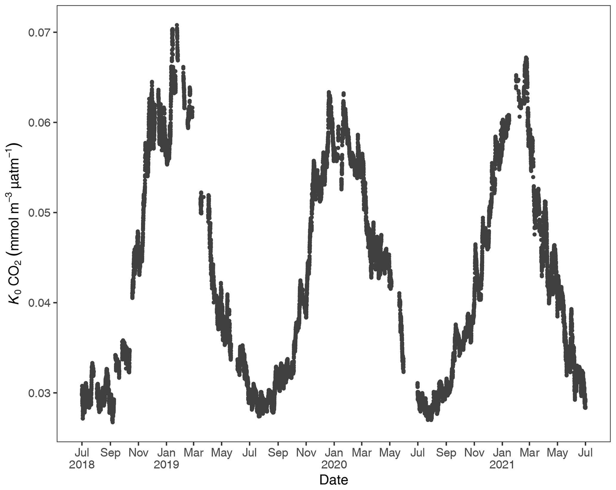
Figure 3Gas-specific solubility (K0) for CO2 based on water temperature and salinity. Units are in the Rhode River (1 July 2018 to 1 July 2021).
Hourly air–water concentration gradient values (ΔC = pCO2 water−pCO2 air) can be inferred by comparison of the measured concentration values across the 3 years of this study (Fig. 2). During warm months, pCO2 water routinely shifts from supersaturated to sub-atmospheric and back again over the course of 24 h (e.g., between >2000 and <410 µatm on a single day). These large daily swings in pCO2 water produced concomitant directional reversals of ΔC (pCO2 water−pCO2 air), which result in longer-term averaged gradients (e.g., multi-day or multi-week averages) near zero (Fig. 2). In contrast, most of the time during cold-water months is spent in a state of sub-atmospheric pCO2 water (under-saturation with respect to the overlying atmosphere), resulting in ΔC values that are negative and that promote movement of CO2 from the atmosphere into the water.
3.3 Gas-specific solubility (K0)
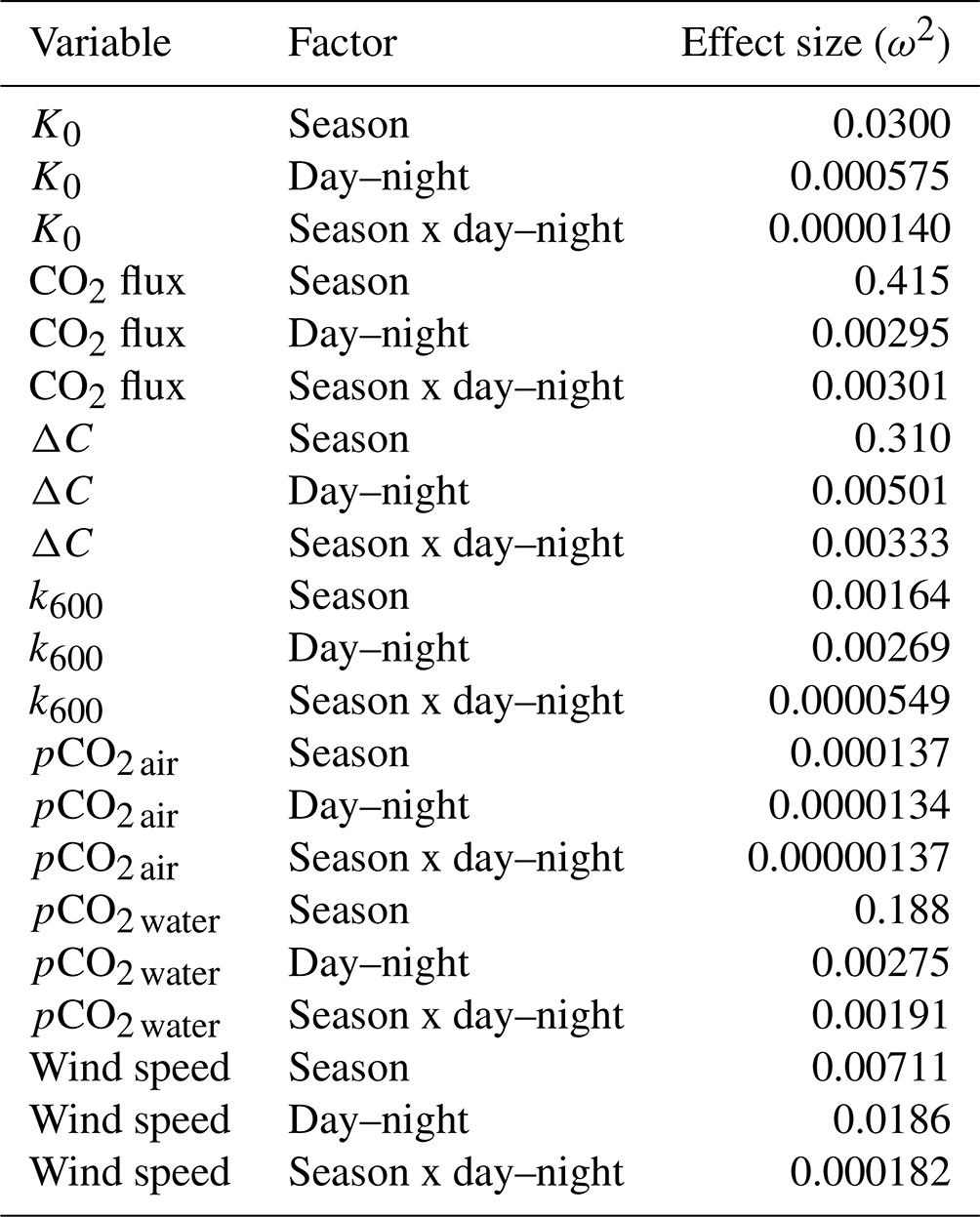
To account for the physical effects of temperature and salinity on the solubility of CO2 in estuarine water, K0 was calculated using the methods of Weiss and Price (1980). K0 varied strongly across seasons over the 3-year observation period. The maximum annual range was 0.027 to 0.071 , mean cold-water months were 0.051, and mean warm-water months were 0.035 , confirming that CO2 was most soluble during winter and least soluble in summer (Fig. 3). This is inverse to observed dissolved CO2 values: pCO2 water was lowest and least variable during winter and highest and most variable during summer (Fig. 2, Table 1), suggesting that solubility in and of itself plays only a minor and non-limiting role in pCO2 water in the Rhode River. Effect size (ω2) estimates indicated that the greatest proportion of variability in K0 was associated with season vs. day–night or the interaction of the two (Table 2).
Table 2Contrast effect sizes based on two-factor ANOVA where independent variables were compared by season (cold-water season, December–May, vs. warm-water season, June–November), day–night period, and the interaction of the two. ω2 is a measure of effect size, estimating the proportion of total variance explained by each parameter. Effect sizes were corrected for inherent temporal autocorrelation using the Cochrane–Orcutt procedure (Spada et al., 2018).
3.4 Temperature–biology ratio
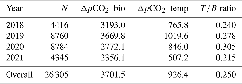
To independently parse the magnitude of the physical vs. biological forcing of pCO2 water, we normalized values to mean water temperature and estimated the Takahashi temperature–biology ratio (Takahashi et al., 2002) to compare the influence of temperature and biological activities on pCO2 water. Across the 3-year period, we found that the predominant driver of pCO2 water in the Rhode River was biological activity, accounting for nearly 4 times more forcing than the physical effects of water temperature on CO2 solubility (Table 3). These patterns demonstrate the outsized role that biological processes play in shaping pCO2 water in nearshore marine and estuarine ecosystems (Dai et al., 2022; Van Dam et al., 2019).
Table 3Takahashi temperature–biology ratio (Eq. 5a from Takahashi et al., 2002).
3.5 Gas transfer velocity (k600)
Gas transfer velocity is affected by both mass transfer from molecular diffusion driven by ΔC (i.e., CO2 gradient between water and the atmosphere) and momentum transfer linked to external environmental forces that enhance turbulence at the air–water boundary layer (Ho et al., 2016; Raymond and Cole, 2001; Van Dam et al., 2019). Van Dam et al. (2019) validated the use of wind speed at 10 m above the water's surface (U10) to estimate gas transfer velocities of CO2 that were standardized to a Schmidt number of 600 (k600) by comparing estimated values to k600 values derived directly from eddy covariance CO2 flux measurements. Given the relative uniformity of wind speed over the Rhode River, where median binned U10 wind speed (converted from U7 measurements) was 2.2 m s−1 regardless of time of day or season and maximum values that rarely exceeded 10 m s−1 (Table 1, Fig. S1), we chose to use the most conservative estuarine-specific parameterization of k600 (Van Dam et al., 2019; Eq. 2). The mean overall Rhode River k600 value for CO2 (mean ± SD, 7.86 ± 2.05 cm h−1) was of comparable magnitude to that of the New River Estuary, NC (9.37 ± 9.47 cm h−1). However, wind speed varied far less on the Rhode River than the New River Estuary and day–night explained more variability in wind speed than season. Because wind speed directly influenced the formulation of k600 (Eq. 2), the effect size of day–night is similarly greater than the seasonal effect on gas transfer velocity (Table 2). Nevertheless, effect sizes (ω2) indicate that season explained at least 10 times more of the observed variance of pCO2 water, pCO2 air, air–water concentration gradient, CO2 flux, and gas-specific solubility than day–night or their interaction (Table 2). Given the minor freshwater input and microtidal nature of the Rhode River, we do not believe that lateral water velocity and bottom turbulence appreciably affect the gas transfer velocity of CO2 here, although we did not investigate possible influences explicitly.
Importantly, in coastal marine and estuarine habitats, ΔC can shift as much as several thousand micro-atmospheres during a single day due to diel cycling associated with CO2 production and depletion (Figs. 2 and S2). The uncertainty surrounding gas transfer velocity parameterization can represent a major source of error in CO2 flux calculations (Frankignoulle et al., 1998; Upstill-Goddard, 2006; Wanninkhof and McGillis, 1999); however, small errors in k600 have far less effect on CO2 flux calculations in estuaries, which experience pCO2 swings of several thousand micro-atmospheres during a single day, compared with more stable conditions of the open ocean where interannual ranges of pCO2 are typically far less (Van Dam et al., 2019).
3.6 CO2 flux–seasonality and interannual variation
CO2 flux was determined according to Eq. (3) using hourly ΔC measurements, CO2 solubility values (K0) calculated according to temperature and salinity, and the estuary-specific standardized gas transfer velocities (k600) of Van Dam et al. (2019). CO2 flux was plotted across the 3 years of observations at hourly and monthly intervals (Fig. 4a and b). As observed with pCO2, CO2 flux in the Rhode River was shown to be strongly seasonal. Given the similarity in wind speed across seasons (Fig. S1), the effect of differential mean ΔC and variation between warm- and cold-water seasons (Fig. 2, Table 1) almost certainly drive the observed seasonal differences in CO2 flux (Fig. 4). Again, the specific solubility of CO2 is greatest at low temperatures, yet this is contrary to the observed mean pCO2 water patterns, pointing toward a biological mechanism for pCO2, ΔC, and ultimately, CO2 flux. The effect size of season on CO2 flux was 2 orders of magnitude greater than either the individual factor of day–night or the interaction of factors, season x day–night (Table 2).
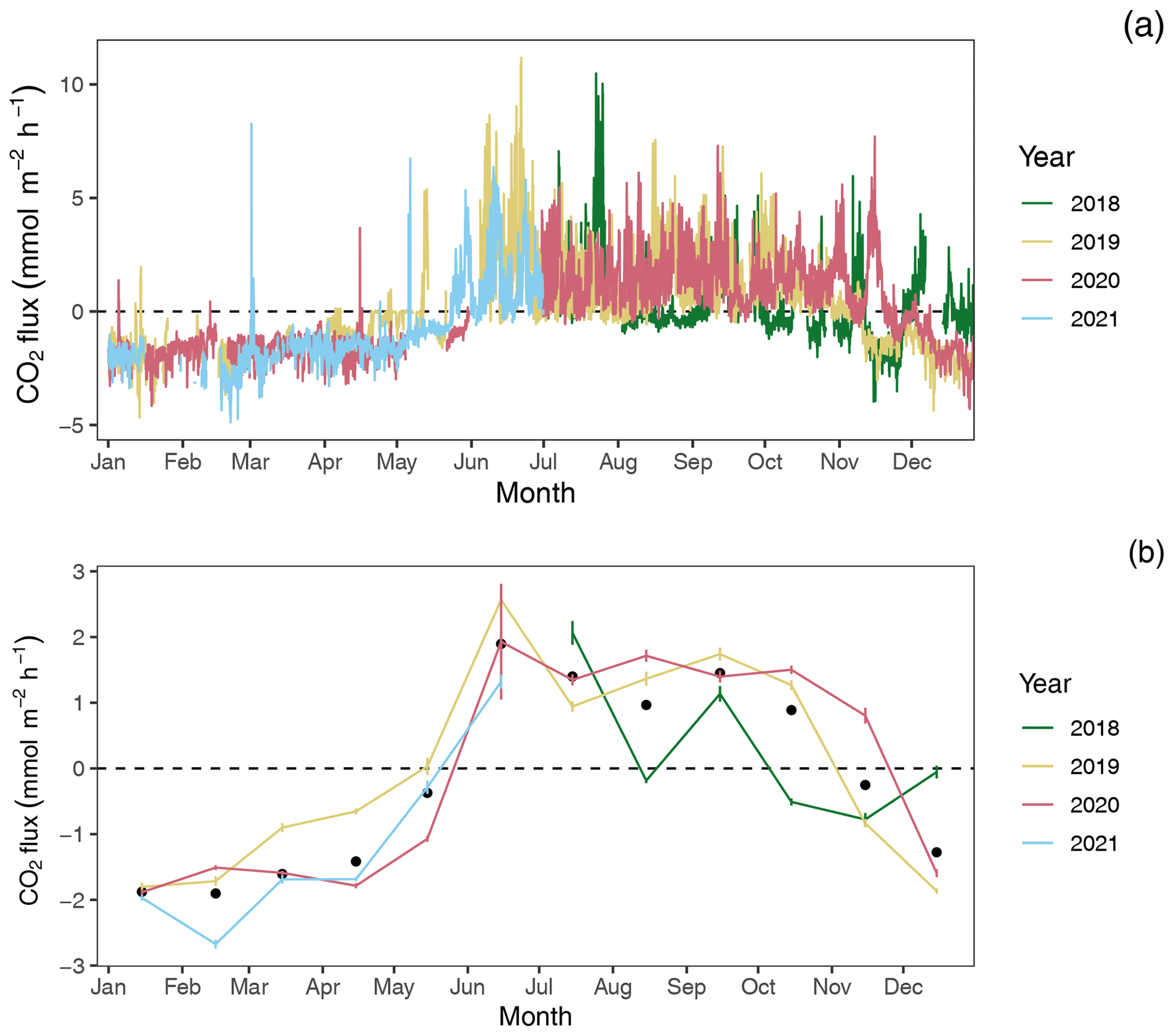
Figure 4CO2 flux estimates by year: (a) hourly and (b) monthly average CO2 flux estimates with 95 % confidence limits. Black dots in panel (b) indicate mean monthly fluxes across years.
Among years, pCO2 water and CO2 flux largely repeat themselves, with dissolved CO2 becoming consistently sub-atmospheric and CO2 flux going negative (gas exchange from atmosphere to water) between December and May and abruptly transitioning to much higher maximum, yet variable, pCO2 water values with net positive CO2 fluxes from June through November (Figs. 2 and 4). Monthly averaged CO2 fluxes are consistent among years (Fig. 4b), with net positive CO2 fluxes (heterotrophic conditions) between June and November and negative (autotrophic) fluxes dominating when water temperatures are cold, between December and May. Despite the overall similarities in seasonal CO2 flux, inter-annual patterns can vary considerably. When hourly CO2 flux values were averaged for the year, the Rhode River in 2019 was shown to have a net positive flux, but it had a net negative flux in 2020. When scaled for the year, 2019 outgassed CO2 from the water to the atmosphere at a rate of 2215.08 (95 % CI = 1816.88, 2613.29). The annual net flux rate in 2020 was negative (i.e., CO2 moved from the atmosphere into the river) at a rate of −1361.31 (95 % CI = −1723.60, −999.01).
At shorter timescales, such as comparing the same week of the year among years, we sometimes observed vast differences in the magnitude and direction of CO2 flux (Fig. S3 in the Supplement), signaling differences in seasonal conditions between years. Transient events can also result in deviations from otherwise typical CO2 flux conditions. For example, the period from July 2018 to January 2019 deviated from other years as CO2 flux was more erratic, with intermittent periods of negative and positive CO2 flux extending later into the winter season than in other years. When water temperatures are compared among years, 2018 was shown to be more inconsistent, with more pronounced temperature shifts and reversals than in 2019 or 2020 (Fig. S1). Salinities remained relatively low for the latter half of 2018 into early 2019, reflecting wetter conditions (Fig. S1). There were also two rapid salinity declines (>4 ppt reductions) in July and October 2018, likely associated with strong precipitation events. These events were both followed by immediate spikes in chlorophyll-a concentration to levels exceeding 200 µg L−1, indicative of phytoplankton bloom conditions. From 2018 to 2021, chlorophyll-a levels of this magnitude and greater were generally confined to cold-water months (December–May; Fig. S1). Erratic water temperature and salinity are also reflected in more variable gas-specific solubility (K0) for CO2 in 2018 than in later years (Fig. 3).
Gallegos et al. (1992) documented predictable phytoplankton blooms associated with freshets in the Rhode River, when nutrient-rich freshwater inundates the estuary not from point and non-point sources within the local Rhode River watershed but instead from the enormous watershed that feeds the Susquehanna River, the primary source of freshwater input into the Chesapeake Bay above the Potomac as well as >50 % of the entire bay's freshwater (US Geological Survey, 2023). Unlike river-dominated estuaries, in the Rhode River estuary, volumetric influxes from the Chesapeake Bay end member far exceed freshwater input from the Muddy Creek and secondary tributaries. In the Rhode River, phytoplankton blooms result in the temporary depletion of pCO2 water, followed by a spike as phytoplankton senesce and organic carbon is decomposed/re-mineralized back into inorganic carbon. Episodic, short-lived occurrences like these demonstrate how immediate small-scale biological forcing can be coupled with and catalyzed by distant large-scale weather and hydrological events. These in turn can influence pCO2 flux variations within seasons and among years (Figs. 3 and S3 and Chen et al., 2020).
Overall, except for wind speed, the effect sizes for the other six measured or calculated variables were shown to be greatest for season vs. day–night or season vs. the interaction of season x day–night, and in all cases the season effect was greater by at least 1 order of magnitude (Table 2). Seasonality has 10 to 1000 times more explanatory power than other variables investigated, as estimated by ω2 (Table 2).
3.7 Shifting net ecosystem production
To better understand how the net ecosystem production (NEP) of the Rhode River shifts throughout the year, where positive NEP indicates that the river is storing carbon (autotrophic state) and negative NEP indicates that it is releasing carbon to the atmosphere (heterotrophic state), we calculated hourly CO2 flux values, averaged them by day (i.e., 24 h period), and plotted each in relation to the ΔC=0 reference. Each day of the 3-year study was categorized as either net heterotrophic (CO2 flux from water to atmosphere) or net autotrophic (CO2 flux from atmosphere to water). Each day was then further identified as purely heterotrophic (all hours of the day were heterotrophic), purely autotrophic, or mixed (some hours were heterotrophic and some were autotrophic, resulting in a net autotrophic or net heterotrophic state for the day; Fig. 5). From July 2018 to July 2021, most 24 h periods were categorized as pure autotrophic ( %), while 25 % () were purely heterotrophic and the remainder of mixed trophic status (17 % net heterotrophic and 10 % net autotrophic; Fig. 5).
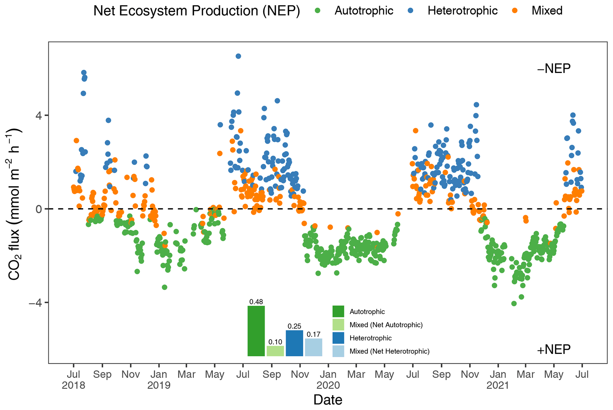
Figure 5Daily mean CO2 flux estimates (the CO2 gradient is CO2 water−CO2 air). Green dots indicate days when all 24 hourly flux measurements were negative (autotrophic with +NEP); blue dots indicate days on which all 24 hourly flux measurements were positive (heterotrophic with −NEP). Orange dots indicate that hourly fluxes were both negative and positive, and the position of the orange dot below or above the zero line indicates whether the day was net autotrophic or net heterotrophic. The insert describes the proportion of days in each category, indicating that during 58 % (0.48+0.10) of days across 3 years of observation, the Rhode River was a CO2 sink.
Altogether, the Rhode River was net autotrophic for 535 of 920 d (58 %) and net heterotrophic for 42 % of the time (385 d) across 3 years. When CO2 flux is integrated over all 3 years, the Rhode River is shown to have near-neutral NEP (Fig. 6). The effect size of season is 2 orders of magnitude greater than either that of day–night or of the season x day–night interaction (Table 2). Mean CO2 flux values highlight the obvious correlation between season and NEP; error bars (±1 SD) reveal the importance of diel cycling where the magnitude and directionality of day–night flux variability is approximately equal to the overall variability accrued across all 3 years (Fig. 6). Although CO2 flux is less variable and more autotrophic during cold-water months than warm-water months in the Rhode River, the range of possible values that occur across night and day, regardless of season, must be taken into consideration to minimize incidental sampling bias (Figs. 2 and 6).
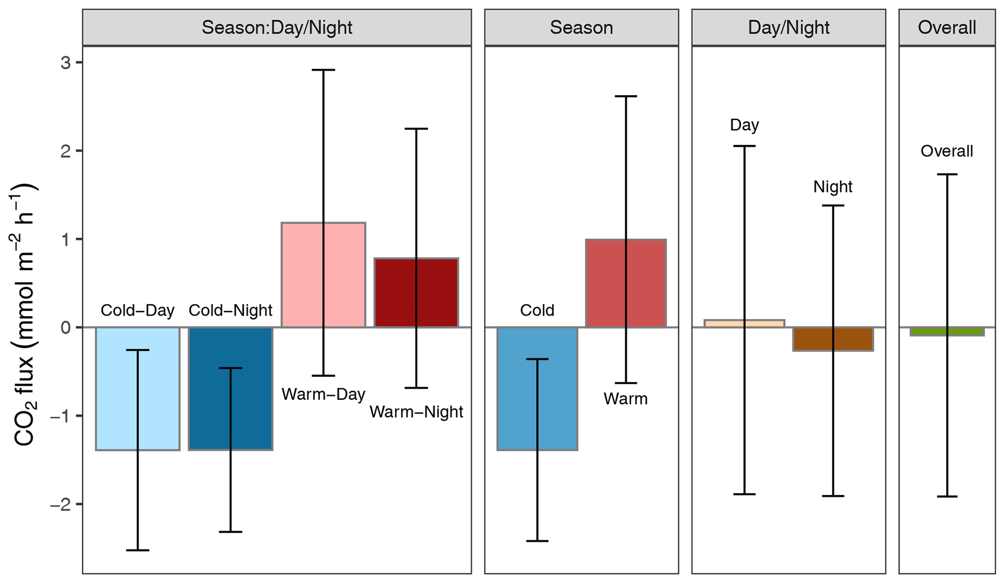
Figure 6Mean CO2 flux ± 1 SD () plotted by day–night cycling, cold-water/warm-water season, season vs. day–night interaction, and overall CO2 flux across 3 years of observation.
A multi-year investigation of CO2 flux in the mainstem of the Chesapeake Bay by Chen et al. (2020) combined several bay-wide cruises that were distributed across seasons to collect discrete and underway pCO2 data for CO2 flux calculations. They concluded that the low-salinity upper bay, which receives large volumes of freshwater from the Susquehanna River, was net heterotrophic; the mesohaline middle bay was net autotrophic, and the polyhaline lower bay was near carbon neutral. Chen et al. (2020) characterized Chesapeake Bay on the whole as a weak source of CO2 to the atmosphere (net flux = 0.73 ) but suggested that during wet years, it may function as weak sink of CO2. Herrmann et al. (2020) also concluded that the Chesapeake Bay was a weak source of CO2 to the atmosphere based on calculated pCO2 values from long-term pH and alkalinity measurements (net flux = 1.2 ). Brodeur et al. (2019) examined dissolved inorganic carbon (DIC) and total alkalinity along the mainstem of the Chesapeake Bay across the year in 2016 and concluded that DIC increases from north to south and from surface waters to depth but that seasonal riverine input and biological cycling were significantly important, concluding that the bay as a whole was a sink for CO2.
When our annual mean pCO2 values were compared with the Chen et al. (2020) survey, the Rhode River was shown to be higher on average and more variable than the mesohaline mainstem of the bay (591 ± 652 vs. 416 ± 167 µatm), including a substantially greater measured range (min=15, max=5182 µatm vs. 103 and 1033 µatm). These results suggest that water in the shallow and well-mixed Rhode River, and DIC in particular, undergo more acute biological transformation than in the mesohaline mainstem of Chesapeake Bay. Chen et al. (2020) point to a variety of factors that affect pCO2 and CO2 flux in the mainstem bay, including temperature, depth, stratification, and freshwater input volume, some of which may attenuate biological forcing. Interannual variability was demonstrated in both the Rhode River (some years were net autotrophic and others heterotrophic; Figs. 4 and 5) and in the mesohaline mainstem of the bay; however, we attribute interannual variability in pCO2 and CO2 flux primarily to variation in water temperature that in turn drives biological activity. We conclude that seasonal variations in the Rhode River (and likely similar rivers in the mesohaline portion of the Chesapeake) are significant and predictable, closely associated with water temperature, and that temperature mediates NEP biologically rather than by changes to the solubility of CO2.
In the Rhode River, we find that CO2 flux reverses itself daily for part of the year (June–November) yielding some days that are characterized as a net sink (net autotrophic) and others that are a net source (net heterotrophic). From December to May, diel cycling is minimal and the river is almost exclusively a net sink, autotrophic both day and night. Finally, although CO2 flux is pronounced but variable across seasons, the net CO2 flux of the Rhode River on an annual basis is near neutral.
3.8 Lateral transport
Tidal cycling has been shown to liberate and laterally transport DOC from brackish marshes to adjacent estuaries (Cai, 2011; Herrmann et al., 2015) and therefore is of great importance to carbon cycling and budgets of wetlands and estuaries (Najjar et al., 2020). DOC outwelling from the Kirkpatrick Marsh (hereafter KPM), a 0.21 km2 tidal marsh located approximately 1 km up estuary from our primary study site at the SERC Dock (Fig. 1), into the Rhode River has been measured and modeled extensively in recent years (Clark et al., 2020; Menendez et al., 2022; Tzortziou et al., 2011, 2008). These studies indicate that the KPM is responsible for a large portion of overall DOC input to the Rhode River, as well as significant export from the river to the mainstem of Chesapeake Bay. Model generation and validation by Clark et al. (2020) indicate that up to 13.1 % of the total DOC input to the Rhode River originates in the KPM. Another important source (53 % of total) is DOC derived from phytoplankton, which is therefore labile and readily biodegraded and remineralized into DIC. Furthermore, large quantities of other semi-labile forms of DOC are exported from the KPM, which are themselves subject to photochemical processes and biodegradation and remineralization (Clark et al., 2020). Importantly, each of these DOC streams provides a potential source of DIC, including pCO2, to the Rhode River.
Dissolved inorganic carbon generated in brackish tidal wetlands is also outwelled directly into estuaries (e.g., Cai et al., 2000; Chu et al., 2018; Song et al., 2023). Recent work by Song et al. (2023) demonstrates that pCO2 in a salt marsh tidal creek in Waquoit Bay, MA, was regulated by both tide height (inversely) and the day–night cycle, with nighttime low tides resulting in the highest pCO2 values, signaling a strong local effect from respiration and photosynthesis in combination with tidal outwelling.
In the Rhode River watershed, pCO2 was measured continuously in the single tidal creek that drains the KPM using the same methods as at our primary study location. We observed that the KPM tidal creek pCO2 follows the tidal cycle exclusively, yet outside the mouth of the tidal creek in the estuary proper, day–night cycling overwhelms this marsh tidal signal. Simultaneous pCO2 measurements from the SERC dock follow a strict day–night cycle (Fig. S4 in the Supplement). However, while peak levels of dissolved CO2 in the Kirkpatrick Marsh creek occur at low tide and can reach values nearly 20 times greater than highs at the SERC dock (Fig. S4), there is no obvious evidence of this tidal DIC input at the dock site. Remineralization of DOC exported from the KPM, as well as DOC originating in other locations within the watershed, are important sources of DIC in the river; however, given the relative volumes of these sources to that of the much larger estuary as well as the physical distance (∼1 km) from SERC dock, these input signals should be expected to lag and be damped inside the estuary and not tightly coupled with tidal cycles. Instead, pCO2 exported from the KPM is expected to undergo significant dilution effects, be partially off-gassed to the atmosphere, and be metabolized via photosynthesis, reducing its influence on downstream sites. These findings suggest that despite periodic extreme pCO2 in KPM tidal creek (>30 000 ppmv), the overall mass of CO2 export is not sufficient to have measurable effects on the deeper, well-mixed portions of the Rhode River.
Thus, although land–sea interfaces and the outwelling of DOC and DIC are important in estuaries and coastal ecosystems, the relative sizes of wetlands and adjacent water bodies and the overall volume of water moving between the two are also important factors. In eutrophic estuaries like the Rhode River, biological forcing can rapidly assimilate DIC and degrade and mineralize labile forms of DOC, as evidenced by extensive diel cycling in these systems (e.g., Brodeur et al., 2019; Song et al., 2023, and the present study.) The much larger and more complex Chesapeake Bay generally follows seasonal changes in pCO2 and CO2 flux, but these appear to be most predictable in the upper oligohaline portion and in the polyhaline region of the bay near the mouth, where freshwater and oceanic end-member effects are most pronounced (Brodeur et al., 2019; Chen et al., 2020). The central mesohaline part of Chesapeake Bay comprises numerous discrete and unique watersheds and sub-estuaries/rivers, each of which exchanges water with the bay. Elucidating spatial and temporal patterns of pCO2 and CO2 flux are vital for understanding each one's role as an atmospheric source or sink but could also provide better insight into how each may be influenced by global increases in atmospheric CO2 (i.e., acidification and its influences on estuarine metabolism and the local biota, fisheries, and habitats each support.) Collectively, these and other sub-estuaries will have cumulative effects on the overall water quality of Chesapeake Bay, including cycling of DOC and DIC, which in turn affect pCO2 and CO2 flux.
The notion that estuaries are predominantly heterotrophic systems that invariably outgas more CO2 to the atmosphere than they absorb has been a long-held view (Abril et al., 2000; Borges et al., 2004; Cai, 2011; Cai et al., 2000; Chen et al., 2013; Frankignoulle et al., 1998; Gattuso et al., 1998). However, more recently investigators have realized that physical and hydrological characteristics, geographical location, size, and biological and biogeochemical activities may individually, or together, influence CO2 flux in estuaries and therefore contributions to atmospheric chemistry (Brodeur et al., 2019; Caffrey, 2004; Chen et al., 2013, 2020; Herrmann et al., 2020). As indicated in this study and others, the role that biological processes play in estuaries to either fix CO2 (autotrophy) or liberate CO2 (heterotrophy) are extensive, complex, and can be quite variable over space and time (Brodeur et al., 2019; Chen et al., 2020; Herrmann et al., 2020; Rosentreter et al., 2021). High-frequency automated measurements revealed strong seasonal contrasts in dissolved CO2 content and CO2 flux between water and the atmosphere of the Rhode River, a shallow mesohaline reach of the Chesapeake Bay. Importantly, only through high-frequency multi-year measurements could diel and seasonal cycling be fully discerned. Indeed, inadequate sampling can induce bias (e.g., upscaling from a small number of daytime samples taken during warm-water months can skew apparent patterns; Laruelle et al., 2017; Van Dam et al., 2019). The timing and frequency of measurements are critical and have potential for strong and misleading biases if sampling is insufficient. In contrast, cold-water months coincide with long periods (weeks to months) of continuous sub-atmospheric sink conditions for CO2. Using these measurements, we estimated the direction and magnitude of CO2 flux in hourly, daily, and annual terms. In the Rhode River, CO2 flux reverses itself daily for part of the year (June through November), yielding some days that are characterized as net sink (net autotrophic and NEP>0) and others that are net source (net heterotrophic and NEP<0). From December to May, diel cycling is minimal, and the river is almost exclusively a CO2 sink with +NEP both day and night. Although CO2 flux is pronounced but variable across seasons, the net CO2 flux of the Rhode River on an annual basis is near carbon neutral, although some years are net heterotrophic and others net autotrophic.
High-frequency sampling of pCO2, although typically confined spatially, is one approach to understanding fundamental aspects of estuarine metabolic states and CO2 flux that may otherwise go undetected (Song et al., 2023). To address the spatial complexity of estuarine, nearshore, and inland waters, more observation locations are required. As with any environmental or ecological question, careful sampling design is critical to balance efficiency and statistical power.
As the largest and arguably most complex estuary in the United States, the Chesapeake Bay is the subject of extensive ecosystem management efforts and ranks among the most studied and monitored estuaries in the world (Boesch and Goldman 2009). Yet, information on CO2 and GHG fluxes continues to be limited (Brodeur et al., 2019; Chen et al., 2020; Herrmann et al., 2020). Given the extensive coordinated monitoring programs that either make real-time water quality measurements and/or maintain routine water sampling schedules (e.g., the Maryland DNR Eyes on the Bay program) in this region, existing water quality observation assets and sampling programs could be leveraged to more fully characterize and quantify CO2 and other GHG dynamics and flux in the bay and elsewhere (see Saba et al., 2019). For example, coordinated deployment of additional automated sampling devices (e.g., robust air–water equilibrators and traditional atmospheric gas sensors) in key locations would enable estimates of CO2 flux, and if combined with pH, DIC, or total alkalinity measurements, carbonate chemistry calculations as well. Importantly, such installations need not be permanent. Instead, a small group of instruments could be systematically deployed across an existing observation network, co-located with other water quality instruments using a stratified sampling approach to capture spatial variability. For example, a set of shifting 2–4-week deployments during summer and winter months could yield sufficient data to advance our understanding of Chesapeake-Bay-wide CO2 flux significantly in a single year. Such information would complement underway transects that are vital but that tend to underestimate temporal variability in any given location. In the case of dissolved GHGs, liquid–air equilibration techniques are being used to measure multiple GHGs (Call et al., 2015; Hartmann et al., 2018; Gülzow et al., 2011; Miller et al., 2019; Xiao et al., 2020).
Understanding the GHG dynamics in estuaries is a vital component to generating accurate global budgets (Maher and Eyre, 2012) as well as informing where emerging carbon capture technologies, including nature-based solutions, might be best located (Bradshaw and Dance, 2005; Sun et al., 2021). In the case of estuaries, there have been extensive global losses of seagrasses due to habitat degradation, pollution, and disease (Waycott et al., 2009). In addition to many other ecosystem service benefits, restoration of seagrass and submerged aquatic vegetation has the potential to restore and enhance natural carbon sequestration (i.e., blue carbon; Kennedy et al., 2022; Macreadie et al., 2022; Unsworth et al., 2022). In Virginia, USA, Oreska et al. (2020) demonstrated how the functional benefits of a restored seagrass meadow habitat can be quantified ecologically in terms of its ability to sequester carbon and affect GHG fluxes between the estuary and atmosphere. Uniquely, these investigators then monetized the costs and benefits of habitat restoration and function as CO2 offset credits as part of a GHG budget and demonstrated how such approaches can be used to incentivize habitat restoration (Oreska et al., 2020).
Increasing the completeness and utility of global GHG budgets as they relate to human activities and ecosystem functions are necessary steps toward combating global climate change. Measurement of GHGs at high spatial and temporal resolution using economical automated measurement solutions can increase our understanding of GHG dynamics at small, ecologically significant scales as well as at the larger ecosystem level of an estuary.
Hourly means of pCO2 and associated environmental data used in the analyses are available at Miller et al. (2023) under Creative Commons license CC BY-NC 4.0.
The supplement related to this article is available online at: https://doi.org/10.5194/bg-21-3717-2024-supplement.
AWM contributed to project conceptualization, funding acquisition, investigation, methodology, project administration, resources, supervision, and writing – original draft. JRM contributed to data curation, formal analysis, software, and visualization. ACR contributed to data curation, investigation, methodology, and project administration. MSM contributed to conceptualization, supervision, and visualization. KJK contributed to conceptualization, data curation, software, and validation. All authors contributed to writing – review and editing.
The contact author has declared that none of the authors has any competing interests.
Publisher's note: Copernicus Publications remains neutral with regard to jurisdictional claims made in the text, published maps, institutional affiliations, or any other geographical representation in this paper. While Copernicus Publications makes every effort to include appropriate place names, the final responsibility lies with the authors.
We thank Patrick Neale and Stephanie Wilson for their early review and critical feedback on this paper, as well as J. Patrick Megonigal for discussions on methodology and the two anonymous reviewers, who contributed beneficial suggestions.
This research has been supported by the Smithsonian Institution (Smithsonian Marine Sciences Network, Johnson Fund).
This paper was edited by Frédéric Gazeau and reviewed by two anonymous referees.
Abril, G. and Borges, A. V.: Carbon Dioxide and Methane Emissions from Estuaries, in: Greenhouse Gas Emissions – Fluxes and Processes: Hydroelectric Reservoirs and Natural Environments, edited by: Tremblay, A., Varfalvy, L., Roehm, C., and Garneau, M., Springer, Berlin, Heidelberg, 187–207, https://doi.org/10.1007/978-3-540-26643-3_8, 2005.
Abril, G., Etcheber, H., Borges, A. V., and Frankignoulle, M.: Excess atmospheric carbon dioxide transported by rivers into the Scheldt estuary, CR Acad. Sci. II A, 330, 761–768, https://doi.org/10.1016/S1251-8050(00)00231-7, 2000.
Bauer, J. E., Cai, W.-J., Raymond, P. A., Bianchi, T. S., Hopkinson, C. S., and Regnier, P. A. G.: The changing carbon cycle of the coastal ocean, Nature, 504, 61–70, https://doi.org/10.1038/nature12857, 2013.
Benson, S., Rich, R., Tashjian, A., Lonneman, M., and Neale, P.: MarineGEO Upper Chesapeake Bay Observatory CPOP Data, https://doi.org/10.25573/SERC.C.6100368.V10, 2023.
Boesch, D. F. and Goldman, E. B.: Chesapeake Bay, USA, in: Ecosystem-Based Management for the Oceans, edited by: McLeod, K. and Leslie, H., Island Press, Washington, D. C., 268–293, ISBN 978-1-59726-155-5, 2009.
Borges, A. V.: Do we have enough pieces of the jigsaw to integrate CO2 fluxes in the coastal ocean?, Estuaries, 28, 3–27, https://doi.org/10.1007/BF02732750, 2005.
Borges, A. V., Delille, B., Schiettecatte, L.-S., Gazeau, F., Abril, G., and Frankignoulle, M.: Gas transfer velocities of CO2 in three European estuaries (Randers Fjord, Scheldt, and Thames), Limnol. Oceanogr., 49, 1630–1641, 2004.
Bradshaw, J. and Dance, T.: Mapping geological storage prospectivity of CO2 for the world's sedimentary basins and regional source to sink matching, in: Greenhouse Gas Control Technologies 7, vol. I, Elsevier, 583–591, https://doi.org/10.1016/B978-008044704-9/50059-8, 2005.
Breitburg, D. L., Hines, A. H., Jordan, T. E., McCormick, M. K., Weller, D. E., and Whigham, D. F.: Landscape patterns, nutrient discharges, and biota of the Rhode River estuary and its watershed: Contribution of the Smithsonian Environmental Research Center to the Pilot Integrated Ecosystem Assessment, https://repository.si.edu/bitstream/handle/10088/18018/serc_BreiteburgEtAl2008RhodeRiverIEA.pdf (last access: 15 December 2023), 2008.
Brodeur, J. R., Chen, B., Su, J., Xu, Y.-Y., Hussain, N., Scaboo, K. M., Zhang, Y., Testa, J. M., and Cai, W.-J.: Chesapeake Bay Inorganic Carbon: Spatial Distribution and Seasonal Variability, Front. Mar. Sci., 6, 99, https://doi.org/10.3389/fmars.2019.00099, 2019.
Broecker, W. S., Takahashi, T., Simpson, H. J., and Peng, T.-H.: Fate of Fossil Fuel Carbon Dioxide and the Global Carbon Budget, Science, 206, 409–418, 1979.
Caffrey, J. M.: Factors controlling net ecosystem metabolism in US estuaries, Estuaries, 27, 90–101, 2004.
Cai, W.-J.: Estuarine and Coastal Ocean Carbon Paradox: CO2 Sinks or Sites of Terrestrial Carbon Incineration?, Annu. Rev. Mar. Sci., 3, 123–145, https://doi.org/10.1146/annurev-marine-120709-142723, 2011.
Cai, W.-J. and Wang, Y.: The chemistry, fluxes, and sources of carbon dioxide in the estuarine waters of the Satilla and Altamaha Rivers, Georgia, Limnol. Oceanogr., 43, 657–668, https://doi.org/10.4319/lo.1998.43.4.0657, 1998.
Cai, W.-J., Wiebe, W. J., Wang, Y., and Sheldon, J. E.: Intertidal marsh as a source of dissolved inorganic carbon and a sink of nitrate in the Satilla River-estuarine complex in the southeastern U. S., Limnol. Oceanogr., 45, 1743–1752, https://doi.org/10.4319/lo.2000.45.8.1743, 2000.
Call, M., Maher, D. T., Santos, I. R., Ruiz-Halpern, S., Mangion, P., Sanders, C. J., Erler, D. V., Oakes, J. M., Rosentreter, J., Murray, R., and Eyre, B. D.: Spatial and temporal variability of carbon dioxide and methane fluxes over semi-diurnal and spring–neap–spring timescales in a mangrove creek, Geochim. Cosmochim. Ac., 150, 211–225, https://doi.org/10.1016/j.gca.2014.11.023, 2015.
Chen, B., Cai, W.-J., Brodeur, J. R., Hussain, N., Testa, J. M., Ni, W., and Li, Q.: Seasonal and spatial variability in surface pCO2 and air–water CO2 flux in the Chesapeake Bay, Limnol. Oceanogr., 65, 3046–3065, https://doi.org/10.1002/lno.11573, 2020.
Chen, C.-T. A., Huang, T.-H., Chen, Y.-C., Bai, Y., He, X., and Kang, Y.: Air–sea exchanges of CO2 in the world's coastal seas, Biogeosciences, 10, 6509–6544, https://doi.org/10.5194/bg-10-6509-2013, 2013.
Chu, S. N., Wang, Z. A., Gonneea, M. E., Kroeger, K. D., and Ganju, N. K.: Deciphering the dynamics of inorganic carbon export from intertidal salt marshes using high-frequency measurements, Mar. Chem., 206, 7–18, https://doi.org/10.1016/j.marchem.2018.08.005, 2018.
Clark, J. B., Long, W., Tzortziou, M., Neale, P. J., and Hood, R. R.: Wind-Driven Dissolved Organic Matter Dynamics in a Chesapeake Bay Tidal Marsh-Estuary System, Estuar. Coast., 41, 708–723, https://doi.org/10.1007/s12237-017-0295-1, 2018.
Clark, J. B., Long, W., and Hood, R. R.: A Comprehensive Estuarine Dissolved Organic Carbon Budget Using an Enhanced Biogeochemical Model, J. Geophys. Res.-Biogeo., 125, e2019JG005442, https://doi.org/10.1029/2019JG005442, 2020.
Correll, D. L., Jordan, T. E., and Weller, D. E.: Nutrient flux in a landscape: Effects of coastal land use and terrestrial community mosaic on nutrient transport to coastal waters, Estuaries, 15, 431–442, https://doi.org/10.2307/1352388, 1992.
Dai, M., Su, J., Zhao, Y., Hofmann, E. E., Cao, Z., Cai, W.-J., Gan, J., Lacroix, F., Laruelle, G. G., Meng, F., Müller, J. D., Regnier, P. A. G., Wang, G., and Wang, Z.: Carbon Fluxes in the Coastal Ocean: Synthesis, Boundary Processes, and Future Trends, Annu. Rev. Earth Pl. Sc., 50, 593–626, https://doi.org/10.1146/annurev-earth-032320-090746, 2022.
Frankignoulle, M., Abril, G., Borges, A., Bourge, I., Canon, C., Delille, B., Libert, E., and Théate, J.-M.: Carbon Dioxide Emission from European Estuaries, Science, 282, 434–436, https://doi.org/10.1126/science.282.5388.434, 1998.
Freeman, L. A., Corbett, D. R., Fitzgerald, A. M., Lemley, D. A., Quigg, A., and Steppe, C. N.: Impacts of urbanization and development on estuarine ecosystems and water quality, Estuar. Coast., 42, 1821–1838, https://doi.org/10.1007/s12237-019-00597-z, 2019.
Gallegos, C. L., Jordan, T. E., and Correll, D. L.: Event-scale response of phytoplankton to watershed inputs in a subestuary: Timing, magnitude, and location of blooms, Limnol. Oceanogr., 37, 813–828, https://doi.org/10.4319/lo.1992.37.4.0813, 1992.
Gallegos, C. L., Jordan, T. E., and Hedrick, S. S.: Long-term Dynamics of Phytoplankton in the Rhode River, Maryland (USA), Estuar. Coast., 33, 471–484, https://doi.org/10.1007/s12237-009-9172-x, 2010.
Gattuso, J.-P., Frankignoulle, M., and Wollast, R.: Carbon and Carbonate Metabolism in Coastal Aquatic Ecosystems, Annu. Rev. Ecol. Syst., 29, 405–434, https://doi.org/10.1146/annurev.ecolsys.29.1.405, 1998.
Gülzow, W., Rehder, G., Schneider, B., Schneider v. Deimling, J., and Sadkowiak, B.: A new method for continuous measurement of methane and carbon dioxide in surface waters using off-axis integrated cavity output spectroscopy (ICOS): An example from the Baltic Sea, Limnol. Oceanogr.-Meth., 9, 176–184, https://doi.org/10.4319/lom.2011.9.176, 2011.
Hartmann, J. F., Gentz, T., Schiller, A., Greule, M., Grossart, H.-P., Ionescu, D., Keppler, F., Martinez-Cruz, K., Sepulveda-Jauregui, A., and Isenbeck-Schröter, M.: A fast and sensitive method for the continuous in situ determination of dissolved methane and its δ13C-isotope ratio in surface waters, Limnol. Oceanogr.-Meth., 16, 273–285, https://doi.org/10.1002/lom3.10244, 2018.
Herrmann, M., Najjar, R. G., Kemp, W. M., Alexander, R. B., Boyer, E. W., Cai, W.-J., Griffith, P. C., Kroeger, K. D., McCallister, S. L., and Smith, R. A.: Net ecosystem production and organic carbon balance of U. S. East Coast estuaries: A synthesis approach, Global Biogeochem. Cy., 29, 96–111, https://doi.org/10.1002/2013GB004736, 2015.
Herrmann, M., Najjar, R. G., Da, F., Friedman, J. R., Friedrichs, M. A. M., Goldberger, S., Menendez, A., Shadwick, E. H., Stets, E. G., and St-Laurent, P.: Challenges in Quantifying Air-Water Carbon Dioxide Flux Using Estuarine Water Quality Data: Case Study for Chesapeake Bay, J. Geophys. Res.-Oceans, 125, e2019JC015610, https://doi.org/10.1029/2019JC015610, 2020.
Ho, D. T., Coffineau, N., Hickman, B., Chow, N., Koffman, T., and Schlosser, P.: Influence of current velocity and wind speed on air-water gas exchange in a mangrove estuary, Geophys. Res. Lett., 43, 3813–3821, https://doi.org/10.1002/2016GL068727, 2016.
Jiang, L.-Q., Cai, W.-J., and Wang, Y.: A comparative study of carbon dioxide degassing in river-and marine-dominated estuaries, Limnol. Oceanogr., 53, 2603–2615, 2008.
Joesoef, A., Huang, W.-J., Gao, Y., and Cai, W.-J.: Air–water fluxes and sources of carbon dioxide in the Delaware Estuary: spatial and seasonal variability, Biogeosciences, 12, 6085–6101, https://doi.org/10.5194/bg-12-6085-2015, 2015.
Jordan, T. E. and Correll, D. L.: Continuous automated sampling of tidal exchanges of nutrients by brackish marshes, Estuar. Coast. Shelf S., 32, 527–545, https://doi.org/10.1016/0272-7714(91)90073-K, 1991.
Jordan, T. E., Correll, D. L., Peterjohn, W. T., and Weller, D. E.: Nutrient flux in a landscape: The Rhode River watershed and receiving waters, in: Watershed Research Perspectives, edited by: Correll, D. L., Smithsonian Institution Press, Washington, DC, https://repository.si.edu/bitstream/handle/10088/17890/serc_Jordan_EtAl1986WtsdPerspectives.pdf (last access: 15 December 2023), 1986.
Jordan, T. E., Correll, D. L., Miklas, J., and Weller, D. E.: Nutrients and chlorophyll at the interface of a watershed and an estuary, Limnol. Oceanogr., 36, 251–267, https://doi.org/10.4319/lo.1991.36.2.0251, 1991.
Kennedy, H., Pagès, J. F., Lagomasino, D., Arias-Ortiz, A., Colarusso, P., Fourqurean, J. W., Githaiga, M. N., Howard, J. L., Krause-Jensen, D., Kuwae, T., Lavery, P. S., Macreadie, P. I., Marbà, N., Masqué, P., Mazarrasa, I., Miyajima, T., Serrano, O., and Duarte, C. M.: Species Traits and Geomorphic Setting as Drivers of Global Soil Carbon Stocks in Seagrass Meadows, Global Biogeochem. Cy., 36, e2022GB007481, https://doi.org/10.1029/2022GB007481, 2022.
Klaus, M. and Vachon, D.: Challenges of predicting gas transfer velocity from wind measurements over global lakes, Aquat. Sci., 82, 53, https://doi.org/10.1007/s00027-020-00729-9, 2020.
Lachin, J. M.: Fallacies of last observation carried forward analyses, Clin. Trials, 13, 161–168, https://doi.org/10.1177/1740774515602688, 2016.
Laruelle, G. G., Goossens, N., Arndt, S., Cai, W.-J., and Regnier, P.: Air–water CO2 evasion from US East Coast estuaries, Biogeosciences, 14, 2441–2468, https://doi.org/10.5194/bg-14-2441-2017, 2017.
Macreadie, P. I., Robertson, A. I., Spinks, B., Adams, M. P., Atchison, J. M., Bell-James, J., Bryan, B. A., Chu, L., Filbee-Dexter, K., Drake, L., Duarte, C. M., Friess, D. A., Gonzalez, F., Grafton, R. Q., Helmstedt, K. J., Kaebernick, M., Kelleway, J., Kendrick, G. A., Kennedy, H., Lovelock, C. E., Megonigal, J. P., Maher, D. T., Pidgeon, E., Rogers, A. A., Sturgiss, R., Trevathan-Tackett, S. M., Wartman, M., Wilson, K. A., and Rogers, K.: Operationalizing marketable blue carbon, One Earth, 5, 485–492, https://doi.org/10.1016/j.oneear.2022.04.005, 2022.
Maher, D. T. and Eyre, B. D.: Carbon budgets for three autotrophic Australian estuaries: Implications for global estimates of the coastal air-water CO2 flux, Global Biogeochem. Cy., 26, GB1032, https://doi.org/10.1029/2011GB004075, 2012.
Martin, C. R., Zeng, N., Karion, A., Dickerson, R. R., Ren, X., Turpie, B. N., and Weber, K. J.: Evaluation and environmental correction of ambient CO2 measurements from a low-cost NDIR sensor, Atmos. Meas. Tech., 10, 2383–2395, https://doi.org/10.5194/amt-10-2383-2017, 2017.
Menendez, A., Tzortziou, M., Neale, P., Megonigal, P., Powers, L., Schmitt-Kopplin, P., and Gonsior, M.: Strong Dynamics in Tidal Marsh DOC Export in Response to Natural Cycles and Episodic Events From Continuous Monitoring, J. Geophys. Res.-Biogeo., 127, e2022JG006863, https://doi.org/10.1029/2022JG006863, 2022.
Miller, A. W., Reynolds, A. C., and Minton, M. S.: A spherical falling film gas-liquid equilibrator for rapid and continuous measurements of CO2 and other trace gases, PLOS ONE, 14, e0222303, https://doi.org/10.1371/journal.pone.0222303, 2019.
Miller, A. W., Muirhead, J. R., Minton, M. S., Reynolds, A. C., and Klug, K. J: Dataset: High frequency, continuous measurements reveal strong diel and seasonal cycling of pCO2 and CO2 flux in a mesohaline reach of the Chesapeake Bay, Smithsonian Environmental Research Center [data set], https://doi.org/10.25573/serc.22491655.v4, 2023.
Najjar, R. G., Herrmann, M., Cintrón Del Valle, S. M., Friedman, J. R., Friedrichs, M. A. M., Harris, L. A., Shadwick, E. H., Stets, E. G., and Woodland, R. J.: Alkalinity in Tidal Tributaries of the Chesapeake Bay, J. Geophys. Res.-Oceans, 125, e2019JC015597, https://doi.org/10.1029/2019JC015597, 2020.
Oreska, M. P. J., McGlathery, K. J., Aoki, L. R., Berger, A. C., Berg, P., and Mullins, L.: The greenhouse gas offset potential from seagrass restoration, Sci. Rep.-UK, 10, 7325, https://doi.org/10.1038/s41598-020-64094-1, 2020.
Raymond, P. A. and Cole, J. J.: Gas Exchange in Rivers and Estuaries: Choosing a Gas Transfer Velocity, Estuaries, 24, 312–317, https://doi.org/10.2307/1352954, 2001.
Raymond, P. A., Hartmann, J., Lauerwald, R., Sobek, S., McDonald, C., Hoover, M., Butman, D., Striegl, R., Mayorga, E., Humborg, C., Kortelainen, P., Dürr, H., Meybeck, M., Ciais, P., and Guth, P.: Global carbon dioxide emissions from inland waters, Nature, 503, 355–359, https://doi.org/10.1038/nature12760, 2013.
Rose, K. C., Neale, P. J., Tzortziou, M., Gallegos, C. L., and Jordan, T. E.: Patterns of spectral, spatial, and long-term variability in light attenuation in an optically complex sub-estuary, Limnol. Oceanogr., 64, S257–S272, https://doi.org/10.1002/lno.11005, 2019.
Rosentreter, J. A., Wells, N. S., Ulseth, A. J., and Eyre, B. D.: Divergent Gas Transfer Velocities of CO2, CH4, and N2O Over Spatial and Temporal Gradients in a Subtropical Estuary, J. Geophys. Res.-Biogeo., 126, e2021JG006270, https://doi.org/10.1029/2021JG006270, 2021.
Saba, G. K., Goldsmith, K. A., Cooley, S. R., Grosse, D., Meseck, S. L., Miller, A. W., Phelan, B., Poach, M., Rheault, R., St.Laurent, K., Testa, J. M., Weis, J. S., and Zimmerman, R.: Recommended priorities for research on ecological impacts of ocean and coastal acidification in the U. S. Mid-Atlantic, Estuar. Coast. Shelf S., 225, 106188, https://doi.org/10.1016/j.ecss.2019.04.022, 2019.
Saucier, W. J.: Principles of Meteorological Analysis, Dover Publications, 468 pp., ISBN 978-0-486-49541-5, 2003.
Song, S., Wang, Z. A., Kroeger, K. D., Eagle, M., Chu, S. N., and Ge, J.: High-frequency variability of carbon dioxide fluxes in tidal water over a temperate salt marsh, Limnol. Oceanogr., 68, 2108–2125, https://doi.org/10.1002/lno.12409, 2023.
Spada, S., Quartagno, M., Tamburini, M., and Robinson, D.: orcutt: Estimate Procedure in Case of First Order Autocorrelation, https://doi.org/10.32614/CRAN.package.orcutt, 2018.
Sun, X., Alcalde, J., Bakhtbidar, M., Elío, J., Vilarrasa, V., Canal, J., Ballesteros, J., Heinemann, N., Haszeldine, S., Cavanagh, A., Vega-Maza, D., Rubiera, F., Martínez-Orio, R., Johnson, G., Carbonell, R., Marzan, I., Travé, A., and Gomez-Rivas, E.: Hubs and clusters approach to unlock the development of carbon capture and storage – Case study in Spain, Appl. Energ., 300, 117418, https://doi.org/10.1016/j.apenergy.2021.117418, 2021.
Takahashi, T., Sutherland, S. C., Sweeney, C., Poisson, A., Metzl, N., Tilbrook, B., Bates, N., Wanninkhof, R., Feely, R. A., Sabine, C., Olafsson, J., and Nojiri, Y.: Global sea–air CO2 flux based on climatological surface ocean pCO2, and seasonal biological and temperature effects, Deep-Sea Res. Pt. II, 49, 1601–1622, https://doi.org/10.1016/S0967-0645(02)00003-6, 2002.
Thoning, K. W., Crotwell, A. M., and Mund, J. W.: NOAA Global Monitoring Laboratory Carbon Cycle and Greenhouse Gases Group Continuous Insitu Measurements of CO2 at Global Background Sites, 1973–Present, https://doi.org/10.15138/YAF1-BK21, 2023.
Tzortziou, M., Neale, P. J., Osburn, C. L., Megonigal, J. P., Maie, N., and JaffÉ, R.: Tidal marshes as a source of optically and chemically distinctive colored dissolved organic matter in the Chesapeake Bay, Limnol. Oceanogr., 53, 148–159, https://doi.org/10.4319/lo.2008.53.1.0148, 2008.
Tzortziou, M., Neale, P. J., Megonigal, J. P., Pow, C. L., and Butterworth, M.: Spatial gradients in dissolved carbon due to tidal marsh outwelling into a Chesapeake Bay estuary, Mar. Ecol. Prog. Ser., 426, 41–56, https://doi.org/10.3354/meps09017, 2011.
Unsworth, R. K. F., Cullen-Unsworth, L. C., Jones, B. L. H., and Lilley, R. J.: The planetary role of seagrass conservation, Science, 377, 609–613, https://doi.org/10.1126/science.abq6923, 2022.
Upstill-Goddard, R. C.: Air–sea gas exchange in the coastal zone, Estuar. Coast. Shelf S., 70, 388–404, https://doi.org/10.1016/j.ecss.2006.05.043, 2006.
U. S. Geological Survey: Freshwater Flow into Chesapeake Bay, https://www.usgs.gov/centers/chesapeake-bay-activities/science/freshwater-flow-chesapeake-bay, last access: 21 September 2023.
Van Dam, B. R., Edson, J. B., and Tobias, C.: Parameterizing Air-Water Gas Exchange in the Shallow, Microtidal New River Estuary, J. Geophys. Res.-Biogeo., 124, 2351–2363, https://doi.org/10.1029/2018JG004908, 2019.
Wanninkhof, R.: Relationship between wind speed and gas exchange over the ocean, J. Geophys. Res.-Oceans, 97, 7373–7382, 1992.
Wanninkhof, R.: Relationship between wind speed and gas exchange over the ocean revisited, Limnol. Oceanogr.-Meth., 12, 351–362, https://doi.org/10.4319/lom.2014.12.351, 2014.
Wanninkhof, R. and McGillis, W. R.: A cubic relationship between air-sea CO2 exchange and wind speed, Geophys. Res. Lett., 26, 1889–1892, https://doi.org/10.1029/1999GL900363, 1999.
Wanninkhof, R., Park, G.-H., Takahashi, T., Sweeney, C., Feely, R., Nojiri, Y., Gruber, N., Doney, S. C., McKinley, G. A., Lenton, A., Le Quéré, C., Heinze, C., Schwinger, J., Graven, H., and Khatiwala, S.: Global ocean carbon uptake: magnitude, variability and trends, Biogeosciences, 10, 1983–2000, https://doi.org/10.5194/bg-10-1983-2013, 2013.
Waycott, M., Duarte, C. M., Carruthers, T. J. B., Orth, R. J., Dennison, W. C., Olyarnik, S., Calladine, A., Fourqurean, J. W., Heck, K. L., Hughes, A. R., Kendrick, G. A., Kenworthy, W. J., Short, F. T., and Williams, S. L.: Accelerating loss of seagrasses across the globe threatens coastal ecosystems, P. Natl. Acad. Sci. USA, 106, 12377–12381, https://doi.org/10.1073/pnas.0905620106, 2009.
Weiss, R. and Price, B.: Nitrous oxide solubility in water and seawater, Mar. Chem., 8, 347–359, https://doi.org/10.1016/0304-4203(80)90024-9, 1980.
Winslow, L. A., Zwart, J. A., Batt, R. D., Dugan, H. A., Woolway, R. I., Corman, J. R., and Read, J. S.: LakeMetabolizer: An R package for estimating lake metabolism from free-water oxygen using diverse statistical models, Inland Waters, 6, 622–636, https://doi.org/10.1080/IW-6.4.883, 2016.
Xiao, S., Liu, L., Wang, W., Lorke, A., Woodhouse, J., and Grossart, H.-P.: A Fast-Response Automated Gas Equilibrator (FaRAGE) for continuous in situ measurement of CH4 and CO2 dissolved in water, Hydrol. Earth Syst. Sci., 24, 3871–3880, https://doi.org/10.5194/hess-24-3871-2020, 2020.
Zeebe, R. E. and Wolf-Gladrow, D.: CO2 in Seawater: Equilibrium, Kinetics, Isotopes, Gulf Professional Publishing, 382 pp., ISBN 978-0-444-50946-8, 2001.
High frequency pCO2 measurements reveal net neutral CO2 flux in a mesohaline reach of the Chesapeake Bay. Net off-gassing to the atmosphere begins in June when water temperatures rise above ~26ºC, continuing through November when temperatures fall below ~10ºC. Dissolved CO2 concentrations follow day–night cycles and are especially pronounced in warm waters. From December through May, the river is largely an uninterrupted sink for CO2 (i.e. CO2 is drawn out of the atmosphere into the river).
High frequency pCO2 measurements reveal net neutral CO2 flux in a mesohaline reach of the...