Evolution of oxygen and stratification and their relationship in the North Pacific Ocean in CMIP6 Earth system models

This study examines the linkages between the upper-ocean (0–200 m) oxygen (O₂) content and stratification in the North Pacific Ocean using four Earth system models (ESMs), an ocean hindcast simulation, and an ocean reanalysis. The trends and variability in oceanic O₂ content are driven by the imbalance between physical supply and biological demand. Physical supply is primarily controlled by ocean ventilation, which is responsible for the transport of O₂-rich surface waters to the subsurface. Isopycnic potential vorticity (IPV), a quasi-conservative tracer proportional to density stratification that can be evaluated from temperature and salinity measurements, is used herein as a dynamical proxy for ocean ventilation. The predictability potential of the IPV field is evaluated through its information entropy. The results highlight a strong O₂–IPV connection and somewhat higher (as compared to the rest of the basin) predictability potential for IPV across the tropical Pacific, where the El Niño–Southern Oscillation occurs. This pattern of higher predictability and strong anticorrelation between O₂ and stratification is robust across multiple models and datasets. In contrast, IPV at mid-latitudes has low predictability potential and its center of action differs from that of O₂. In addition, the locations of extreme events or hotspots may or may not differ between the two fields, with a strong model dependency, which persists in future projections. On the one hand, these results suggest that it may be possible to monitor ocean O₂ in the tropical Pacific based on a few observational sites co-located with the more abundant IPV measurements; on the other, they lead us to question the robustness of the IPV–O₂ relationship in the extratropics. The proposed framework helps to characterize and interpret O₂ variability in relation to physical variability and may be especially useful in the analysis of new observation-based data products derived from the BGC-Argo float array in combination with the traditional but far more abundant Argo data.

1 Introduction

Dissolved oxygen (O₂) in the oceans is crucial for biogeochemical cycling, marine ecosystems, and the redox chemistry of seawater. O₂ is a key element for the survival and functioning of marine organisms, as fish, shellfish, marine mammals, and other aquatic life rely on O₂ to breathe and carry out essential metabolic processes. Growth, reproduction, and the overall health of marine organisms depend on the balance between metabolic demands and O₂ supply (Deutsch et al., 2015).

Ocean deoxygenation refers to the long-term decrease in the concentration of O₂ in the Earth's oceans. At the global scale, according to historical observations, the O₂ inventory has been declining significantly during the past decades (Ito et al., 2017; Schmidtko et al., 2017). Changes in O₂ concentrations can reflect the impacts of climate change, nutrient pollution, eutrophication, and other human-induced stressors (e.g., Breitburg et al., 2018). Predicting O₂ levels in the oceans is especially important around and within oxygen minimum zones (OMZs), which are characterized by layers in the water column with very low O₂ concentration due to biological, chemical, and physical processes. As oceans warm, OMZs are posed to increase in number and size across the globe, thereby threatening marine ecosystems. In the North Pacific, a large OMZ exists on the eastern side of the tropical Pacific, and its variability and trends are important for nitrogen cycling and the production of N₂O, a potent greenhouse gas (Nevison et al., 2003; Yang et al., 2017). However, O₂ measurements are temporally and spatially sparse, and trends remain uncertain: the decline in O₂ between 1970 and 2010 is estimated to be around −0.48 ± 0.35 % per decade in the upper 1000 m (Bindoff et al., 2019). The uncertainty in ocean deoxygenation estimates is due to different interpolation methods, data quality control standards, and data sources, the latter varying from shipboard measurements (ship-based bottle measurements and CTD–O₂ profiles) to biogeochemical Argo floats (Roemmich et al., 2019).

Interpreting changes in O₂ concentrations requires an understanding of how ocean circulation, mixing, air–sea gas exchange, biological productivity, and respiration operate. The air–sea gas exchange for O₂ is relatively efficient, and it maintains the surface water close to saturation with the overlying atmosphere for ice-free regions. Ocean circulation is the primary pathway through which O₂ is supplied (or ventilated) into the thermocline and deep ocean. At the subsurface, O₂ is gradually consumed by respiration due to the decomposition of dissolved and particulate organic matter. The O₂ concentration progressively decreases as water masses age. At the climatological timescale, the rates of O₂ supply and consumption are balanced to sustain a steady state. In another words, changes in O₂ concentration are caused by an imbalance between O₂ supply and O₂ consumption. On the supply side, the ventilation of O₂ is essentially controlled by ocean circulation and mixing processes. Broadly, ventilation refers to the exchange of water between the surface layer and the ocean's interior (Talley et al., 2011) and involves a wide range of physical processes such as the wind-driven shallow overturning associated with subtropical cells (Brandt et al., 2015; Duteil et al., 2014; Eddebbar et al., 2019), the formation of mode and intermediate waters (Claret et al., 2018; Sallée et al., 2010, 2012; Gnanadesikan et al., 2012), and lateral (isopycnal) eddy stirring (Rudnickas et al., 2019; Gnanadesikan et al., 2013, 2015). These circulation systems are ultimately driven by atmospheric winds and air–sea buoyancy fluxes, which exhibit significant interannual, decadal, and multi-decadal variability. Fluctuations in ventilation rates as well as in ocean stratification are known to impact both O₂ levels (Ridder and England, 2014; Duteil et al., 2014; McKinley et al., 2004) and the distribution of isopycnal potential vorticity (IPV), a dynamical tracer which is proportional to the local stratification and the Coriolis parameter. Use of the absolute value of the Coriolis parameter in the formula, as indicated by ∗, guarantees that the relationship with stratification holds with the same sign in both hemispheres, so a higher IPV^* indicates stronger stratification and vice versa. A strong wintertime convective mixing will produce weakly stratified O₂-rich water masses (low IPV^* and high O₂) and vice versa. These properties are then brought together into the ocean's interior following the pathway of large-scale ocean currents.

In this study, we build upon this relationship and explore the overarching hypothesis that IPV^* may be used as a proxy for O₂ with a focus on the North Pacific basin. If this is the case, then IPV^* may provide a means to monitor and predict the evolution of O₂. In the North Pacific, the Pacific Decadal Oscillation (PDO) is the mode of climate variability that exerts the greatest control on stratification and O₂, as shown by Ito et al. (2019). Indeed, the dominant mode of oxygen variability in the North Pacific Ocean is correlated with the PDO index such that the PDO explains about 25 % of its variance. In the tropics, the PDO modulates the depths of isopycnal surfaces and biological productivity and respiration together with the El Niño–Southern Oscillation (ENSO), while at mid-latitudes it is the dominant mode influencing the depth of winter-mixed-layer ventilation and ventilation processes. Here we analyze outputs from the Coupled Model Intercomparison Project Phase 6 (CMIP6; Eyring et al., 2016), a major international effort with the primary objective of providing a standardized framework for simulating past, present, and future climate conditions. The participating modeling groups run their climate models under prescribed forcing fields and following a common protocol, thereby generating a comprehensive set of output datasets which are freely available to the scientific community through data portals and archives provided by the Earth System Grid Federation (ESGF). Using a suite of Earth system models (ESMs) run with prescribed carbon dioxide concentrations, we address the following questions:

• How robust is the relationship between O₂ and IPV^* in the North Pacific across several ESMs and how may it evolve by the end of the 21st century (related to HYP 1; see below)?

• What are the linkages between O₂ and IPV^* and large-scale modes of climate variability such as PDO and ENSO (related to HYP 2)?

• Where are the hotspots of changes in IPV^* and O₂ in the historical period and in the projections, and are they co-located or do they differ in space and time (related to HYP 3)?

Our specific objectives are to evaluate the hypotheses that ocean ventilation (IPV^*) regulates O₂ variability in the North Pacific (HYP 1); that the PDO/ENSO–ventilation–O₂ linkage provides the basis for the predictability of O₂ whenever IPV^* is predictable (HYP 2); and that the linkage can be exploited to identify hotspots of changes in O₂ variability, means, and extremes (HYP 3; see “Materials and methods”). While testing these hypotheses, we also aim to introduce recently developed approaches for model intercomparison and data analysis to the ocean biogeochemistry community. Specifically, in this work we adopt the information entropy (IE; Prado et al., 2020) concept for evaluating predictability, a data-mining tool for dimensionality reduction and network analysis (δ-MAPS; Fountalis et al., 2018), and the standard Euclidean distance (SED) index (Diffenbaugh and Giorgi, 2012) to evaluate changes in the fields we analyze. In short, IE is a metric that measures the amount of randomness and therefore unpredictability in a dataset. For example, if a time series is a random sequence, its entropy will be high, while if a time series follows a sinusoidal curve, its IE will be low. On the other hand, δ-MAPS combines feature extraction and network analysis into a single framework. Its goal is to identify key features and to visualize how those features relate to one another. Finally, the SED index is a simple and flexible method used to detect total changes in one or more variables in a given dataset (in other words, to identify regions that stand out for changes in means, extremes, and variability) through measuring the distance in multi-variate space between a baseline period and any other. After introducing these tools in more detail in Sect. 2, a description of the data analyzed in this work follows in Sect. 3. Results are then presented in Sect. 4, with a general discussion and conclusions to close.

2 Materials and methods

In this section, we describe the three tools recently developed for climate science applications and adopted in our analysis as well as how we calculate IPV^*. The information entropy (IE) is used to evaluate predictability. IE is defined following Prado et al. (2020) and is based on the recurrence of microstates in a recurrence plot (RP). An RP (Eckmann et al., 1987) is a visualization technique for trajectory recurrence of a given dynamical system described in phase space by a matrix R_ij such that

$$\begin{array}{}\text{(1)}& {\mathbf{R}}_{ij}\left(\mathit{ϵ}\right)=\mathrm{\Theta }\left(\mathit{ϵ}-\left|{\mathit{x}}_i-{\mathit{x}}_j\right|\right),{\mathit{x}}_i\in R^d,ij=\mathrm{1},\mathrm{2},\mathrm{\dots },K,\end{array}$$

where Θ is the Heaviside function; $\left|\right|$ is an Euclidean distance; x_i and x_j are, in our work, states at time steps i and j; ε is a threshold distance (the maximum distance between two states to be considered mutually recurrent); d is the x_i space dimension; and K is the number of states considered (the length of each analyzed time series). R_ij is a matrix that represents non-recurrent (as zeros) and recurrent (as ones) states in phase space, and it is explicitly dependent on ε. Corso et al. (2018) introduced the recurrence entropy quantifier, for which for a given time series, the probability of occurrence of microstates in its RP is quantified without the need for a space-state reconstruction. A microstate of dimension N is an N by N matrix sampled inside the RP, with a probability of occurrence $P_k=n_k/N_{\mathrm{tot}}$, where n_k is the number of occurrences of the microstate and N_tot is the total number of possible configurations of 0 and 1 of the microstate (see Ikuyajolu et al., 2021, and Prado et al., 2020, for more details). The IE is then defined as

$$\begin{array}{}\text{(2)}& \mathrm{IE}\left(N_{\mathrm{tot}}\right)=-{\sum }_{k=\mathrm{1}}^{N_{\mathrm{tot}}}{P}_k\ln P_k,\end{array}$$

where k refers to the kth microstate. When IE is normalized by the maximum entropy (corresponding to when all microstates show the same probability), then IE = 0 corresponds to perfect predictability and IE = 1 represents chaos. Furthermore, the explicit dependence of the entropy quantifier on ε is removed using the maximum entropy formulation. Prado et al. (2020) have shown that a value for which IE is maximum exists, does not vary much with varying ε, and is strongly correlated with the Lyapunov coefficient of the system. We refer the reader to Ikuyajolu et al. (2021) for details of the heuristic used to estimate the maximum entropy. In essence, Prado et al. (2020) suggest a technique to eliminate the dependence of the entropy computation on the selection of a distance threshold ε by finding a clearly defined maximum (S_max) in the relationship between ε and the entropy (see Fig. 4 in Prado et al., 2020). This maximum is robust and relatively stable within a range of ε values. Furthermore, there is a strong correlation between the maximum entropy and the Lyapunov exponent. In our work, the code used to compute the entropy (see the “Code and data availability” section) uses the heuristic explained in Ikuyajolu et al. (2021) for the calculation of S_max through an iterative procedure that calculates the recurrence entropy for varying ε until a maximum is found and retained. This algorithm requires three input parameters: the microstate dimension (set at 4 in this work, but we explored other values as shown in the Results section), the number of random samples to compute the microstate distribution in the RP (here 10 000), and a random sub-sample used to determine the ε value for which the entropy is maximum (here 1000). We compute the entropy field of the deseasonalized and detrended IPV^* (full signal) using monthly data over all historical and future periods. At each point, the entropy of the IPV^* field is associated with recurring microstates in its time series (which defines the system and thereby impacts its predictability). The higher the predictability of a time series is, the more recurrent its temporal dynamics are, i.e., the easier it will be to predict its future evolution.

δ-MAPS (Fountalis et al., 2018) is used to identify climate modes of variability. It is an unsupervised network analysis method that identifies spatially contiguous and possibly overlapping regions referred to as domains and the lagged functional relationships between them. This dimensionality-reduction method is simpler and easier to interpret than empirical orthogonal functions (EOFs), which suffer from orthogonality constraints (Dommenget and Latif, 2002). Its benefits relative to conventional EOF-based approaches include interpretability and prevention of overfitting when extracting climate patterns from high-dimensional datasets (Falasca et al., 2019). In short, δ-MAPS domains are spatially contiguous regions that share a highly correlated temporal activity between grid cells. In this work, we apply δ-MAPS to the sea surface temperature (SST) anomaly field (see the “Code and data availability” section) to identify major modes of climate variability in the North Pacific in a reanalysis and in the ESMs. Given any spatiotemporal field, its local homogeneity is hypothesized to be highest at “epicenters” or “cores”. For each grid point, a local homogeneity is defined as the average pairwise cross-correlation between that grid cell and a set of K nearest neighbors (see Fountalis et al., 2018, for details). Cores are then determined as neighbors of points where the local homogeneity is a local maximum and above a threshold δ. Each core is iteratively expanded and merged using a greedy algorithm to iteratively find domains as large as possible that are (i) spatially contiguous, (ii) include at least one core, and (iii) have homogeneity higher than δ. Using a significance test, δ is computed for the unlagged cross-correlations. Given any random pair of grid points, the significance of the Pearson correlation of their time series is assessed through Bartlett's formula (Box et al., 2011), with the null hypothesis of no coupling. The significance of each correlation is tested for a user-specified significance level α, and δ is computed as the average of the significant correlations. Here, we applied δ-MAPS with K=8 and α=0.01.

Lastly, we adopt the approach introduced by Diffenbaugh and Giorgi (2012) (which builds on Williams et al., 2007; Diffenbaugh et al., 2008; and references therein) to identify hotspots of change. The SED is a non-parametric method, meaning that it does not assume a specific probability distribution for the data. This flexibility makes it applicable to a wide range of datasets, regardless of their underlying distribution. The reader is referred to Turco et al. (2015) for its application to global atmospheric data. Here we apply the procedure described in Turco et al. (2015) to O₂ and IPV^* as follows: hotspots are quantified through a standard Euclidean distance (SED) index that aggregates the changes in means, variability, and extremes of the given spatiotemporal field according to

$$\begin{array}{}\text{(3)}& \mathrm{SED}=\sqrt{{\sum }_{i=\mathrm{1}}^{N\mathrm{\Delta }}{\sum }_{j=\mathrm{1}}^{\mathrm{4}}{\left({\displaystyle \frac{{\mathrm{\Delta }}_{ij}}{p_{\mathrm{95}}\left(\left|{\mathrm{\Delta }}_{ij}\right|\right)}}\right)}^{\mathrm{2}}}.\end{array}$$

We compute two SED indices in each grid point, separately for O₂ and IPV^*. N_Δ is the total number of indicators per variable and i is the index identifying each indicator; j spans the seasons, so Δ_ij is the ith indicator in the jth season; and p₉₅ is the 95th percentile. The indicators and SEDs are computed point by point; i.e., each grid point has one value. Therefore, the percentile is computed spatially over all the grid points. Here we consider December–January–February (the boreal) winter, March–April–May spring, and so on. We consider three indicators for each variable, evaluating changes in means, variability, and extremes between two periods of equal length. Period 1 covers 1950 to 1981 (1960 to 1986 for the reanalysis and the E3SM-2G ocean hindcast). Period 2 covers 1983 to 2014 (1988 to 2014 for the reanalysis and the hindcast) over the historical time frame and 2036 to 2067 and 2069 to 2100 for the projected future. In Eq. (3), indicators of both periods are normalized to the 95th percentile calculated over period 1 to fairly compare changes in the intensity of hotspots over time. We chose not to compare the period from 2069 to 2100 with the period from 1950 to 1981 but rather to compare it to 2036 to 2067 instead because we wish to track changes in each period compared to the preceding time slot to quantify how rapidly they occur in the future projections compared to the historical time frame. For each variable, we compute three indicators at each grid point and for each season using the Climate Data Operators (CDO; Schulzweida, 2022) as follows.

Changes in means are estimated in each season separately by ${\mathrm{\Delta }}_{\mathrm{means}}={\mathrm{yseasm}}_{\mathrm{2}}-{\mathrm{yseasm}}_{\mathrm{1}}$, where yseasm₁ and yseasm₂ are the multi-year seasonal means in periods 1 and 2, respectively. Therefore, taking for example the O₂ historical simulations over the period from 1950 to 2014 (although similar expressions also hold for IPV^* and the other periods), ${\mathrm{\Delta }}_{\mathrm{means}\mathrm{DJF}}=\langle {\mathrm{O}}_{\mathrm{2}\mathrm{DJF}}{\rangle }_{\mathrm{1983}\text{–}\mathrm{2014}}-\langle {\mathrm{O}}_{\mathrm{2}\mathrm{DJF}}{\rangle }_{\mathrm{1950}\text{–}\mathrm{1981}}$, ${\mathrm{\Delta }}_{\mathrm{means}\mathrm{MAM}}=\langle {\mathrm{O}}_{\mathrm{2}\mathrm{MAM}}{\rangle }_{\mathrm{1983}\text{–}\mathrm{2014}}-\langle {\mathrm{O}}_{\mathrm{2}\mathrm{MAM}}{\rangle }_{\mathrm{1950}\text{–}\mathrm{1981}}$, ${\mathrm{\Delta }}_{\mathrm{means}\mathrm{JJA}}=\langle {\mathrm{O}}_{\mathrm{2}\mathrm{JJA}}{\rangle }_{\mathrm{1983}\text{–}\mathrm{2014}}-\langle {\mathrm{O}}_{\mathrm{2}\mathrm{JJA}}{\rangle }_{\mathrm{1950}\text{–}\mathrm{1981}}$, and ${\mathrm{\Delta }}_{\mathrm{means}\mathrm{SON}}=\langle {\mathrm{O}}_{\mathrm{2}\mathrm{SON}}{\rangle }_{\mathrm{1983}\text{–}\mathrm{2014}}-\langle {\mathrm{O}}_{\mathrm{2}\mathrm{SON}}{\rangle }_{\mathrm{1950}\text{–}\mathrm{1981}}$, where 〈…〉 is a time mean (seasonal climatology).

Changes in multi-year seasonal variability Δ_variability are evaluated by (i) detrending each variable point by point in the two periods separately; (ii) computing the multi-year seasonal standard deviation of these detrended fields, yseasσ, for each period for each season; and (iii) computing as the percent changes such that ${\mathrm{\Delta }}_{\mathrm{variability}}=\mathrm{100}\cdot \left(\frac{\mathrm{yseas}{\mathit{\sigma }}_{\mathrm{2}}-\mathrm{yseas}{\mathit{\sigma }}_{\mathrm{1}}}{\mathrm{yseas}{\mathit{\sigma }}_{\mathrm{1}}}\right)$. Therefore, with the example of O₂ historical simulations over the period from 1950 to 2014, ${\mathrm{\Delta }}_{\mathrm{variability}\mathrm{DJF}}=\mathrm{100}\left(\mathrm{std}\right({\mathrm{O}}_{\mathrm{2}\mathrm{DJF}}{)}_{\mathrm{1983}\text{–}\mathrm{2014}}-\mathrm{std}\left({\mathrm{O}}_{\mathrm{2}\mathrm{DJF}}{)}_{\mathrm{1950}\text{–}\mathrm{1981}}\right)/\mathrm{std}({\mathrm{O}}_{\mathrm{2}\mathrm{DJF}}{)}_{\mathrm{1950}\text{–}\mathrm{1981}}$, where std(…) is the multi-year seasonal (winter) standard deviation over the specified period (equivalent formulations also hold for the other seasons).

Finally, changes in extremes (in our case overshoots of IPV^* and undershoots of O₂) are computed through the following steps: (i) for each season, we compute at each grid point the multi-year O₂ minimum or IPV^* maximum over period 1 using monthly data (e.g., the O₂ minimum given all December, January, and February values for the boreal winter), and we build a threshold map for each season; (ii) we count how many times O₂ < threshold${}_{{\mathrm{O}}_{\mathrm{2}}}$ (or IPV^* > threshold${}_{{\mathrm{IPV}}^{\ast }}$) is verified in each corresponding season of period 2, again using monthly data; and (iii) the percentage of occurrences computed in point (ii) is finally taken as an indicator of percent changes in extremes and estimated by ${\mathrm{\Delta }}_{\mathrm{extremes}}=\mathrm{100}\times \left(\frac{N_{\mathrm{occ}}}{N_{\mathrm{T}}}\right)$, where N_occ is the number of extreme occurrences (in each season) and N_T is the total number of months in the corresponding seasons (96 for the models and 81 for reanalysis and hindcast).

Building on previous works (Falasca et al., 2019; Falasca and Bracco, 2022), we expect the statistics of a given model to remain relatively stable across ensemble members; i.e., we do not expect the member choice to significantly influence the calculation of extremes and hotspots or their relationships in particular. We verified that this is indeed the case in one of the models by testing four additional randomly chosen ensemble members of CanESM5 (see the “Code and data availability” section). A major advantage of this hotspot definition is that it accounts for changes in the mean, variability, and extremes at the same time. In other words, it accounts for the intrinsic characteristics of the simulated climate fields, which can be characterized by considering all three aspects together. In particular, the definition of extremes aims at including information on months exceeding corresponding seasonal baseline extremes, without choosing a threshold on the current distribution a priori, which is especially relevant for comparing changes with respect to a reference baseline. The three indicators, grouped into four seasons for each variable, are then used to compute the SED indices.

Finally, IPV^* (m⁻¹ s⁻¹) is used as a proxy for stratification and is defined as the isopycnic potential vorticity (Talley et al., 2011) with the absolute value of the Coriolis parameter in its formula:

$$\begin{array}{}\text{(4)}& {\mathrm{IPV}}^{\ast }={\displaystyle \frac{\left|f\right|}{g}}{N}^{\mathrm{2}}.\end{array}$$

Here, N² is the Brunt–Väisälä frequency ($-\frac{g}{\mathit{\rho }}\frac{\partial \mathit{\rho }}{\partial z})$, which measures the fluid stability to vertical displacements; g is the gravitational acceleration; f is the Coriolis parameter; and ρ is the density, calculated in this work using salinity and temperature fields and the TEOS-10 equation of state for seawater (http://www.teos-10.org/, last access: 17 April 2024). IPV is a conservative tracer in frictionless and adiabatic circulation. IPV^* is calculated over the three-dimensional ocean volume using Eq. (4) considering the 0–200 m vertical weighted average. This procedure allows us to compare datasets with different vertical discretization.

3 Data

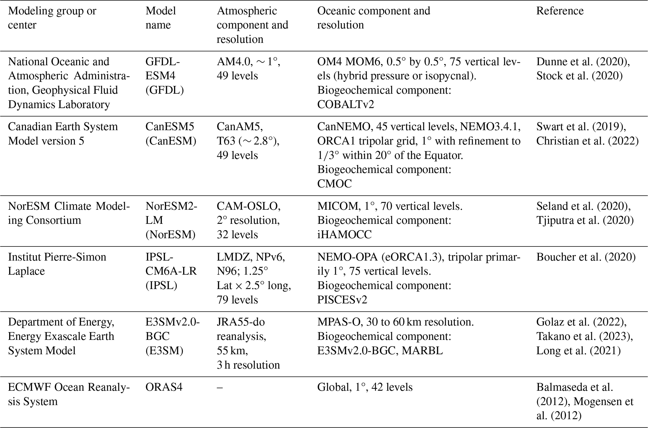
We consider four ESMs from the CMIP6 historical catalogue (with prescribed CO₂ concentrations), a hindcast, and reanalysis data, as summarized in Table 1. Whenever multiple ensemble members were available, we selected the first (r1i1p1f1). We randomly selected four additional ensemble members for CanESM5 (r5i1p1f1, r10i1p1f1, r15i1p1f1, and r20i1p1f1) to further verify the robustness of the hotspot calculation to the member choice. All ESMs are forced with prescribed CO₂ concentrations from 1850 to 2014, and we analyze the monthly outputs from 1950 to 2014. We further discuss future SSP5-8.5 scenarios and focus on the 2036 to 2100 period, indicated as future.

The hindcast is a new ocean–ice biogeochemistry simulation (referred to as the G-Case) E3SMv2.0-BGC (hereafter E3SM-2G; Takano et al., 2023) based on the Model for Prediction Across Scales – Ocean (MPAS-O), an ocean component of the Energy Exascale Earth System Model (E3SM) version 2 (Golaz et al., 2022). Details on ocean physics updates can be found in Golaz et al. (2022). One of the major updates is the introduction of Redi isopycnal mixing (Redi, 1982). Along with ocean physics updates, this version also incorporated a uniform background vertical diffusion specifically developed for simulations of the ocean biogeochemistry to enhance ocean carbon uptake and thermocline ventilation of dissolved inorganic carbon (DIC). Incorporating this mixing parameterization results in improved representation of climatological O₂ distributions in the v2.0 version compared to its predecessor (Burrows et al., 2020). The Marine Biogeochemistry Library (MARBL; Long et al., 2021) is used to simulate ecosystem dynamics and the cycling of biogeochemical elements. After the spin-up period, the model is forced by a meteorological reanalysis dataset, JRA55-do version 1.4 (Tsujino et al., 2020), from 1958 onward. As an ocean reanalysis, we use the ORAS4 product (Balmaseda et al., 2012; Mogensen et al., 2012) available from 1959 onward, which includes a direct surface flux implementation from ERA-40 and ERA-Interim and multi-scale bias correction. When analyzing the E3SM-2G hindcast and the ORAS4 reanalysis, we focus on the 1960 to 2014 interval to avoid the spurious presence of an anticyclonic tropical cyclone in the northeastern Pacific in 1959 in JRA55-do v1.4.

All the data, models, and reanalysis are remapped at 1° by 1° horizontal resolution and to a common vertical grid with a linear interpolator.

Table 1 The CMIP6 Earth system models, global ocean hindcast, and reanalysis used in this work. Under each model name, a short form used in the following figures is indicated in parentheses.

We begin our analysis with a brief evaluation of the ESM biases in the two main fields of interest, IPV^* and O₂. For IPV^*, the ocean reanalysis dataset is used for validating the model outputs for the maximum possible time overlap in the historical configuration (1959 to 2014). For O₂, we can only contrast the annual mean O₂ climatology data between the World Ocean Atlas (Garcia et al., 2019) and the ESMs (Fig. 1). We additionally compared the ORAS4 IPV^* climatology data over the period from 1988 to 2014 (i.e., period 2 for this reanalysis) with the corresponding climatology data computed using SODA3.4.2, which uses a different ocean component to ORAS4. The differences across reanalyses that use different models but assimilate the same observations are much smaller (about 1 order of magnitude) than the signal (Fig. S1 in the Supplement) and smaller than any model bias.

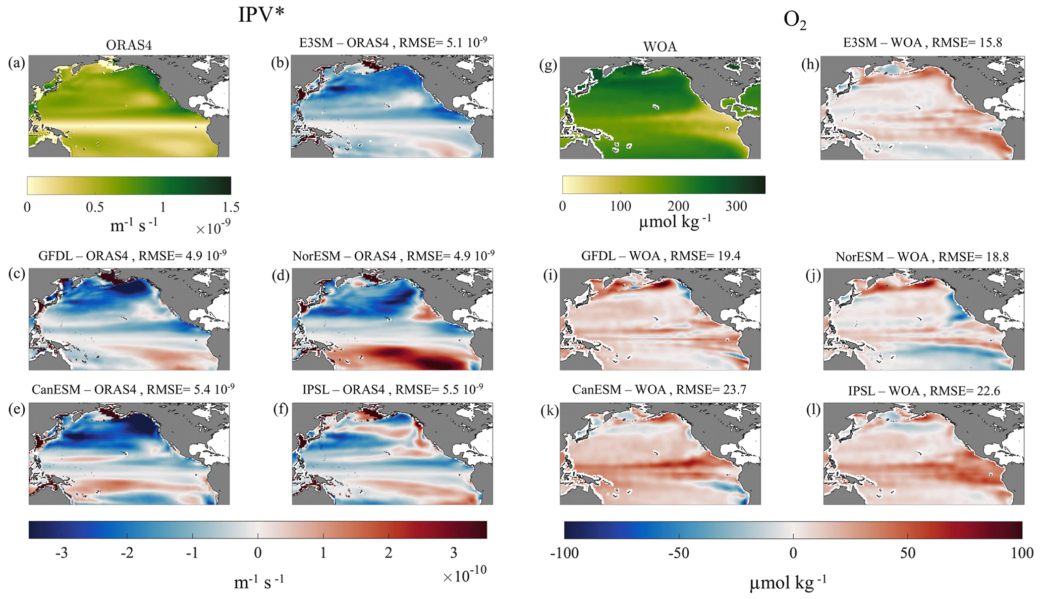
Figure 1 (Left) IPV^* annual climatology means (1959 to 2014) weighted-averaged over 0–200 m depth in the North Pacific basin. (a) ORAS4. (b–f) Model bias (model − ORAS4) differences. (Right) O₂ annual climatology means (1950 to 2014) weighted-averaged over 0–200 m depth. (g) World Ocean Atlas (WOA) climatology means. (h–l) Model biases (model − WOA) difference. The root mean square error (RMSE) values of the modeled IPV^* (m⁻¹ s⁻¹) and O₂ (µmol kg⁻¹) are shown for each panel.

The E3SM-2G hindcast is forced by observed atmospheric fields and displays the smallest bias and, for O₂, also the smallest root mean square error (RMSE), which is shown atop the panels in Fig. 1. Overall, the IPV^* and O₂ biases have broadly anticorrelated patterns, with the models being generally less stratified and more oxygen rich than observed in the extratropical North Pacific and often too stratified and with a larger O₂ deficit compared to observations south of the Equator. However, maximum and minimum biases in the two fields seldom coincide. Regionally, E3SM-2G is generally less stratified than observed, with a relatively low O₂ bias and an overestimation of approximately 10 µmol kg⁻¹ in the subtropical thermocline of the North Pacific basin. The hindcast performs especially well in the tropical thermocline. Among the CMIP6 models, CanESM5 shows a slightly higher IPV^* underestimation in the subpolar gyre and an O₂ overestimation in the subtropics compared to the other ESMs, while NorESM2-LM emerges as the most stratified south of the Equator. For O₂, larger biases (positive or negative) are generally found in the tropical thermocline and the tropical and subtropical boundaries. The sign and magnitude of the biases are model dependent. Interestingly, models generally overestimate O₂ at subpolar latitudes.

4 Results

4.1 Predictability potential (HYP 1)

We begin our analysis by considering the predictability potential of IPV^* as quantified through the information entropy (IE; see “Materials and methods”). The goal is to verify if and where IPV^* has an elevated predictability owing to the presence of quasi-recurrent behaviors in its time series. We also aim to examine whether O₂ is correlated with IPV^* in regions where the latter has a high predictability potential. As a reminder, IE values close to 1 indicate high complexity and unpredictability, and values close to 0 indicate perfect predictability (the signal is recurrent, e.g., constant or periodic). We preliminarily tested the sensitivity of the entropy field to the microstate dimension within a range that is meaningful according to previous literature (Ikuyajolu et al., 2021) using microstates of dimensions 2, 3, 4, and 5 for GFDL over the period from 1950 to 2014 (Fig. S2). We found that the IE pattern, i.e., areas more (or less) predictable relative to the surroundings, is substantially unchanged and that the geographical patterns are robust to changes in the microstate dimension, in agreement with Ikuyajolu et al. (2021). Both microstate dimension 4 and microstate dimension 5 show reasonable entropy values, and we chose to use a microstate dimension of 4 to conduct our analysis because it spans the widest range of possible values.

4.1.1 O₂–IPV^* relationship across ESMs and its future evolution

IE maps for IPV^* are shown in Fig. 2 for both historical and future time frames, with superposed contours of the areas where the (lagged) anticorrelation between IPV^* and O₂ is at least −0.5 (see Figs. S3–S4 for the anticorrelation and lag maps). Higher predictability in the historical period is found in the tropical Pacific areas close to the geographical location of ENSO (i.e., the area most impacted by the domain identified as ENSO-related by δ-MAPS, which maps well the region identified by an EOF analysis over the SST field for having the greatest variance explained by the first principal component, pc1). The predictability potential is generally highest along two stripes enclosing the ENSO pattern north and south of the Equator and excluding the upwelling cold tongue. The distribution of IE follows broadly that found in a much longer simulation of the IPSL model covering the past 6000 years and analyzed by Falasca et al. (2020), and it appears to be robust across models. The western boundary current region and the Kuroshio–Oyashio Extension have low predictability across all datasets considered. In NorESM2-LM and CanESM5, and to a lesser degree in ORAS4 and IPSL-CM6A-LR, the higher predictability of the ENSO area extends to the northeastern portion of the basin. In general, in both the hindcast and the models, strong anticorrelations between IPV^* and O₂ (correlation coefficient (c.c.) ≤ −0.5) coincide with regions of low IE and are linked to ENSO affecting stratification and O₂ concurrently in the tropics and south of the upwelling area. Very limited IPV^* predictability is found in the central and western North Pacific, where the variability is dominated by the PDO signal. The PDO does not emerge as easily predictable in the interval considered, in agreement with, e.g., Gordon et al. (2021) and Falasca et al. (2020), who analyzed the predictability of sea surface temperatures in the IPSL model across the whole second half of the Holocene. In those areas, anticorrelations between O₂ and IPV^* are relatively weak (generally > −0.4 except for NorESM). The entropy and the regions where the evolution of IPV^* and O₂ are strongly anticorrelated do not change significantly in the future projections of the four models. We further explored whether oxygen solubility (O_2sol), which is modulated by ocean warming and cooling, and the apparent oxygen utilization (AOU), which is controlled mostly by the biogeochemical processes affecting oxygen demand, may be independently linked to IPV^* predictability. The areas in which IPV^* and AOU time series are positively correlated, with correlation coefficients ≥ 0.5, are very similar to the ones obtained by analyzing the O₂–IPV^* relationship. For O_2sol, which approximates preformed O₂ at the depths considered well, the anticorrelation areas (i.e., where c.c. ≤ −0.5) are quite extensive, especially in the hindcast, but mostly superimposed onto high-entropy and low-predictability IPV^* areas (Fig. S5).

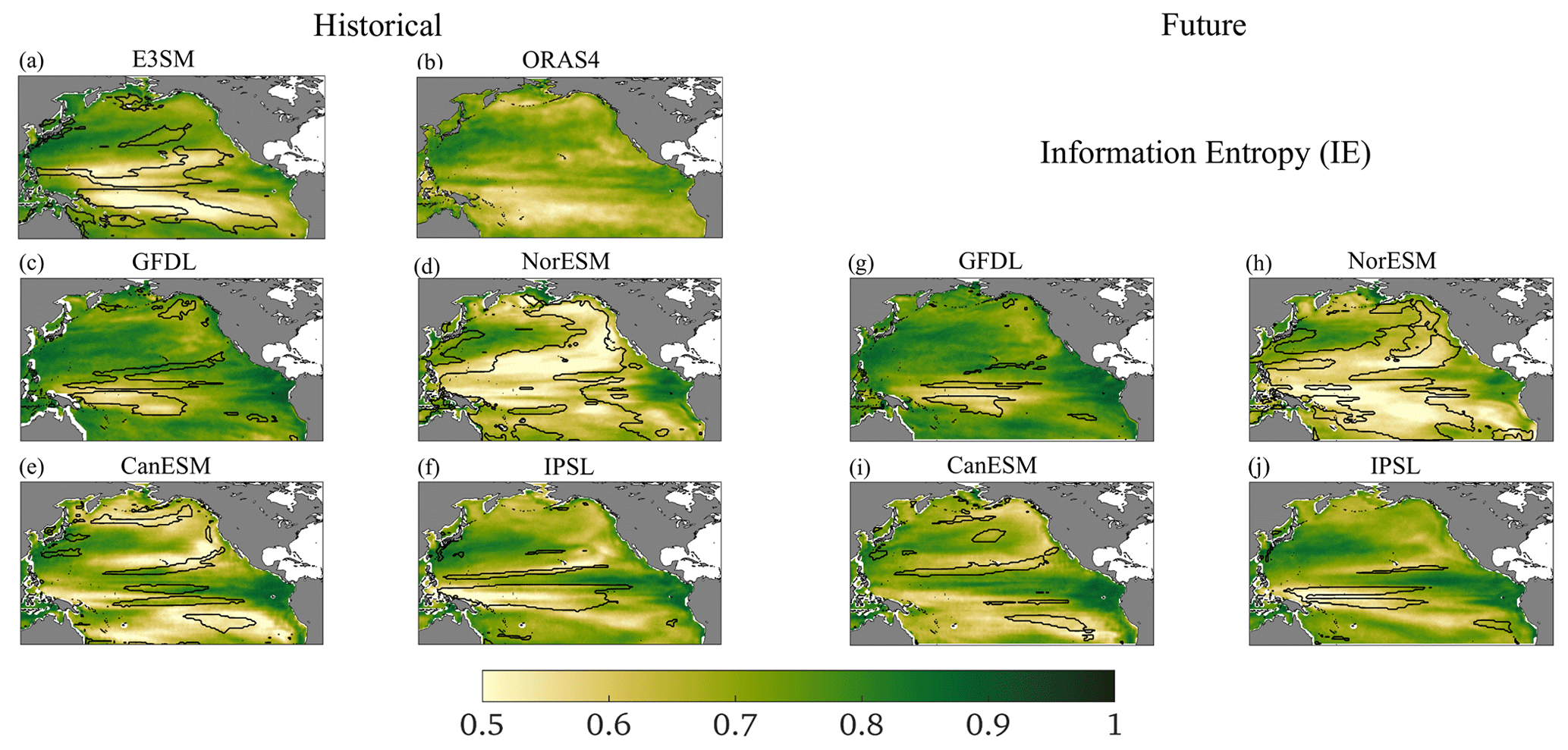
Figure 2 IPV^* information entropy in the historical interval (left) and in the future (right) for the ESMs and in the historical period from 1960 to 2014 for the hindcast and ORAS4, with superposed contours of the areas where in which the IPV^* and O₂ time series are anticorrelated, including correlation coefficients $\le -\mathrm{0.5}$.

In Fig. S6 we show the IE maps for O₂. Predictability is generally higher outside the equatorial upwelling region and the Kuroshio–Oyashio Extension. In E3SM, the areas in which the predictability potential of IPV^* is high and the correlation with O₂ is ≤ 0.5 coincide and also have low IE in O₂. This is verified to some extent in IPSL and NorESM but not in the other two models.

In the next section we isolate the PDO signal to explore whether the low predictability in the North Pacific (north of ENSO region) is related to the superposition of different timescales, i.e., whether there is low-frequency PDO modulation with high-frequency “noise” due to both atmospheric and oceanic variability. The PDO is indeed a lower-frequency mode compared to ENSO and has most loading at extratropical latitudes in which the atmospheric “noise” is greater.

4.2 Trends and PDO impact on O₂ and IPV^* (HYP 2)

The limited predictability found in the North Pacific does not exclude the possibility of the PDO modulating both IPV^* and O₂ inventories simultaneously. As explored in previous work (e.g., Ito et al., 2019), the dominant mode of observed O₂ variability in the northern Pacific Ocean is indeed correlated with the PDO index, which explains about 25 % of the variance. Observations, however, offer only sparse coverage in both time and space. To further verify the PDO modulation, we computed the first EOF for the E3SM-2G hindcast 0–200 m O₂ and IPV^* anomalies for the period from 1960 to 2014 over the northern Pacific (20.5–69.5° N  115.5° E–60.5° W) and the corresponding time series for pc1. The first EOF explains 25 % of the oxygen variance and about 12 % of the IPV^* variance. The computed pc1 shows a significant and strong correlation (Pearson's R coefficient) with the PDO time series computed using SST anomalies, with $\left|R\right|=\mathrm{0.83}$ (p<0.01) for O₂ and $\left|R\right|=\mathrm{0.44}$ (p<0.01) for IPV^* after applying 5-year moving means. The correlation with the PDO is higher than with the ENSO, which is at most $\left|R\right|=\mathrm{0.34}$ (p<0.01) for O₂ after applying a 3-month moving mean, consistent with the analysis by Ito et al. (2019). We hereby quantify the (linear) impact of the PDO on the two fields of interest and then evaluate their residuals. If the PDO is the main predictor of IPV^* and O₂ distributions, its impact on the two fields should be strongly anticorrelated and larger than the residual. As mentioned above, the objective is to verify whether IPV^* could be used to extrapolate information about O₂ and its evolution in time, bypassing – at least to some degree – the need to run full biogeochemical models or measure O₂ directly.

4.2.1 Estimation of climate indices and their relationship with IPV^* and O₂

We use δ-MAPS (see “Materials and methods”) applied to the SST field to evaluate the main modes of Pacific climate variability, i.e., ENSO and PDO, and their time evolution in the models, in the ocean hindcast, and in the reanalysis. While the evolution of ENSO using δ-MAPS is straightforwardly described by the time series of the cumulative anomalies in the ENSO-related domain (e.g., Falasca et al., 2019), for the PDO we must consider the difference between the SST cumulative anomalies of two domains. The domains are identified by the complex network algorithm, and we applied a 5-year running mean to produce the PDO time series shown in Fig. 3. The shape and size of the domains are indicated in Fig. 4. For ORAS4 and E3SM-2G over the period from 1960 to 2014, we computed the 0-lag Pearson's correlation coefficients between these time series and the commonly defined indices of PDO (following Mantua et al., 1997) and Niño 3.4 (average SST anomalies over the box 5° N–5° S, 170–120° W) retrieved from NOAA (https://psl.noaa.gov/data/climateindices/list/, last access: 17 April 2024). After applying a 3-month moving average to the ENSO time series (signals and indices) and a 5-year moving average to the PDO time series (signals and indices), the correlation coefficients are 0.88 for PDO and 0.93 for ENSO in ORAS4 and 0.89 for PDO and 0.91 for ENSO in E3SM-2G.

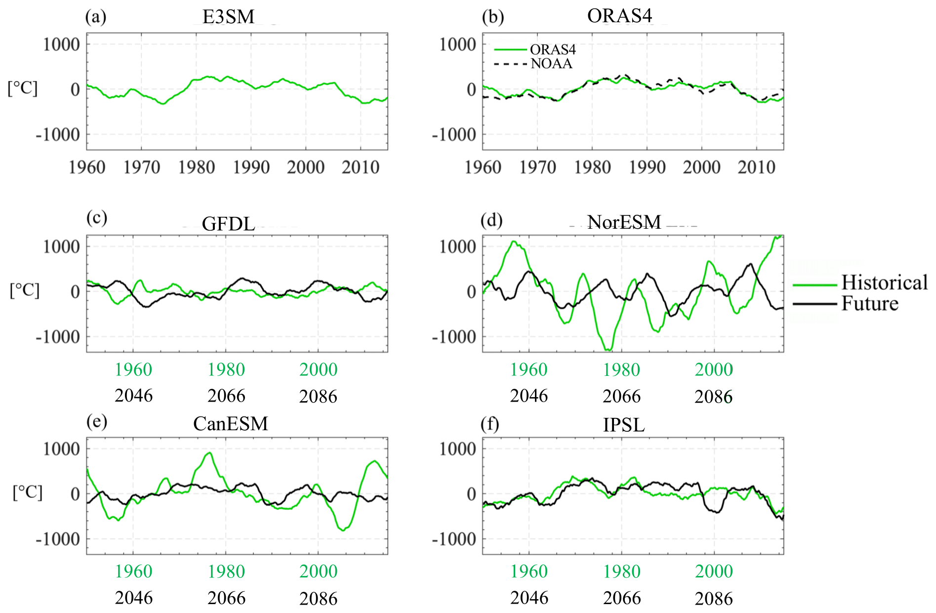
Figure 3 PDO indices (SST cumulative anomalies) calculated using δ-MAPS (see text) in the historical and future time frames. The dashed line in panel (b) is the PDO index time series from NOAA (available at https://psl.noaa.gov/data/climateindices/list/, last access: 17 April 2024) multiplied by the standard deviation of the ORAS4 time series in panel (b) after applying a 5-year moving mean.

Among the models (Fig. 3), GFDL slightly underestimates the PDO strength during the historical period, while the opposite is true of CanESM and NorESM. In the latter, the frequency of the signal is also higher than observed. By the end of the 21st century, the strength of the PDO remains unaltered in GFDL and IPSL, while it decreases in NorESM2 and especially in CanESM following a decrease in the size of the eastern domain. A decrease in amplitude and an increase in frequency of the PDO were also found in several models in the CMIP5 ensemble (Li et al., 2020).

Given the PDO(t) indices, the residual component of the fields of interest that is not linearly forced by the PDO can be separated as a function of time (see, e.g., Kucharski et al., 2008) so that for O₂ (but the same procedure was applied to IPV^*)

$$\begin{array}{}\text{(5)}& {\mathrm{O}}_{\mathrm{2}\mathrm{res}}(x,y,t)={\mathrm{O}}_{\mathrm{2}}(x,y,t)-{\mathrm{O}}_{\mathrm{2}\mathrm{PDO}}(x,y,t),\end{array}$$

where

$$\begin{array}{}\text{(6)}& {\mathrm{O}}_{\mathrm{2}\mathrm{PDO}}(x,y,t)=b_{{\mathrm{O}}_{\mathrm{2}}}(x,y)\cdot \mathrm{PDO}\left(t\right).\end{array}$$

The parameter $b_{{\mathrm{O}}_{\mathrm{2}}}(x,y)$ is constant over time and determined by least-squares fitting through a linear regression for each dataset separately. Figure 4 shows $b_{{\mathrm{IPV}}^{\ast }}$ and $b_{{\mathrm{O}}_{\mathrm{2}}}$ for all datasets with the boundaries of the domains corresponding to the ENSO mode and those contributing to the PDO in the historical period superposed. In most cases there is an overall anticorrelation between the maps of the two fields, but there are also several important differences. First, the regions in which $b_{{\mathrm{O}}_{\mathrm{2}}}$ is strongest (both positive and negative values) do not correspond to minima and maxima in $b_{{\mathrm{IPV}}^{\ast }}$. Second, the equatorial upwelling tends to have a strong positive signal in $b_{{\mathrm{O}}_{\mathrm{2}}}$ and only a weak one, albeit of the same sign, in $b_{{\mathrm{IPV}}^{\ast }}$. Third, the impacts of PDO on the fields vary substantially among models, as quantified by the correlations among the respective fields indicated atop the $b_{{\mathrm{O}}_{\mathrm{2}}}$ plots, with GFDL being the closest to the hindcast and, for the IPV^* case, also to the reanalysis. In NorESM2 the anticorrelation between the regression fields is too strong and the PDO has both a shape and a loading different to those observed in the Pacific interior. CanESM and IPSL display positive spatial correlations, with important biases with respect to the hindcast at the Equator and along the eastern boundary.

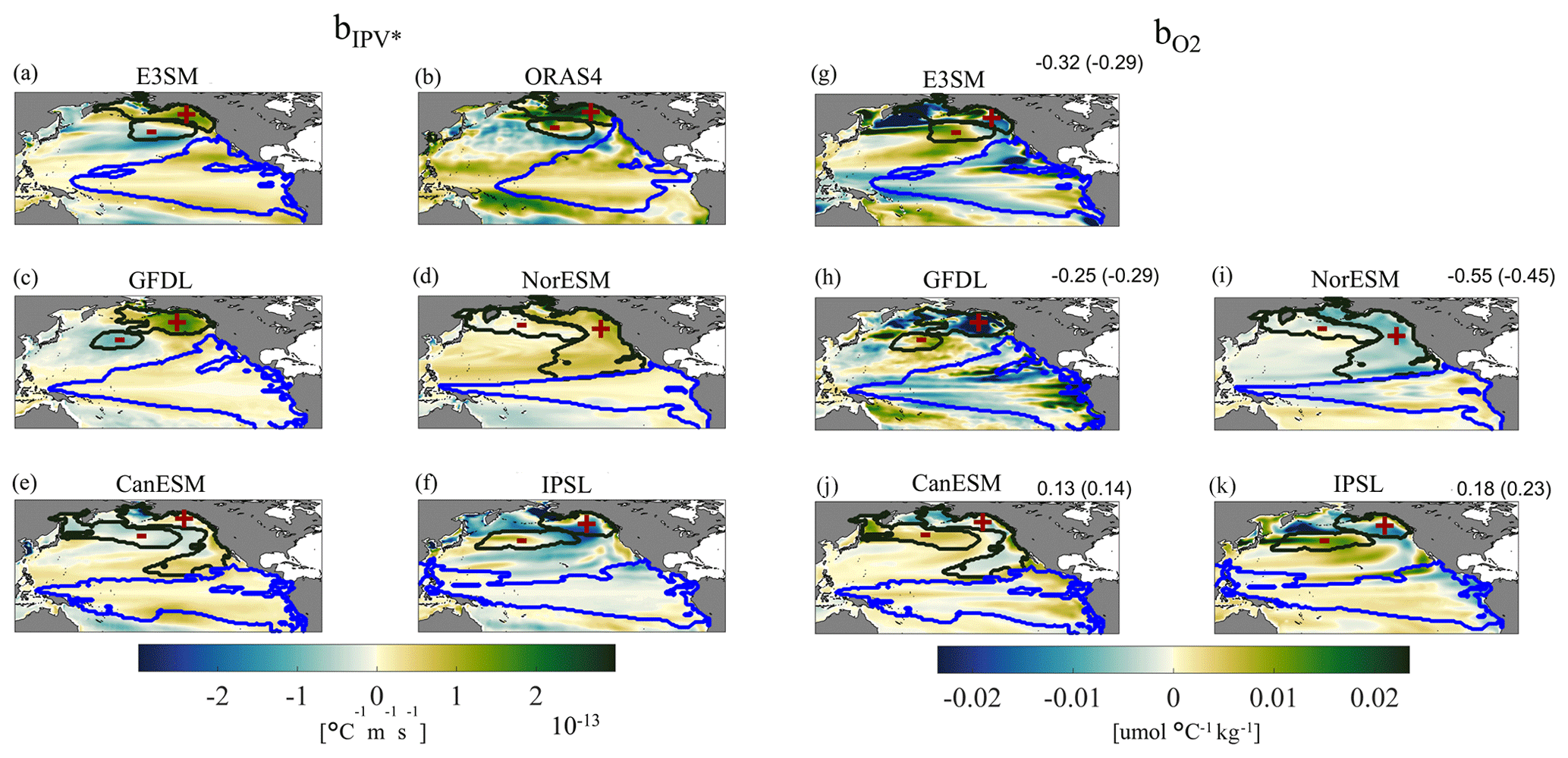
Figure 4 $b_{{\mathrm{IPV}}^{\ast }}$ (left) and $b_{{\mathrm{O}}_{\mathrm{2}}}$ (right) regression coefficient maps with superposed contours of the ENSO (blue line) and of the PDO+ and PDO− domains. $b_{{\mathrm{IPV}}^{\ast }}$ represents the change in IPV^* per unit change in SST, and $b_{{{\mathrm{O}}_{\mathrm{2}}}^{\ast }}$ represents the change in O₂ per unit change in SST. The correlation coefficients (c.c.'s) among the corresponding maps for the same model or hindcast are also indicated. Color limits are fixed as ±3 standard deviations of the ensemble for each variable over the whole area ($\pm \mathrm{2.99}\times {\mathrm{10}}^{-\mathrm{13}}$ for IPV^* and ±0.023 for O₂). Values in parentheses are c.c.'s computed north of 20° N. All c.c.'s passed a shuffling significance test at the 5 % level (see Supplement).

We performed a comparable linear regression analysis using the ENSO index instead of the PDO and, as expected, obtained similar shapes of the b coefficients but much lower absolute values (Fig. S8). This further confirms that in the North Pacific, the PDO is the dominant mode of climate variability.

Moving on to the projections, the maps of the regression coefficients do not change considerably in three of the models considered (Fig. 5). In CanESM, on the other hand, $b_{{\mathrm{IPV}}^{\ast }}$ changes sign over most of the domain. The residual trends, when compared to the regression coefficients, are stronger and dominate the evolution of both fields, especially in the subtropical and subpolar gyres of the North Pacific (Fig. S9), thereby superseding the PDO signal.

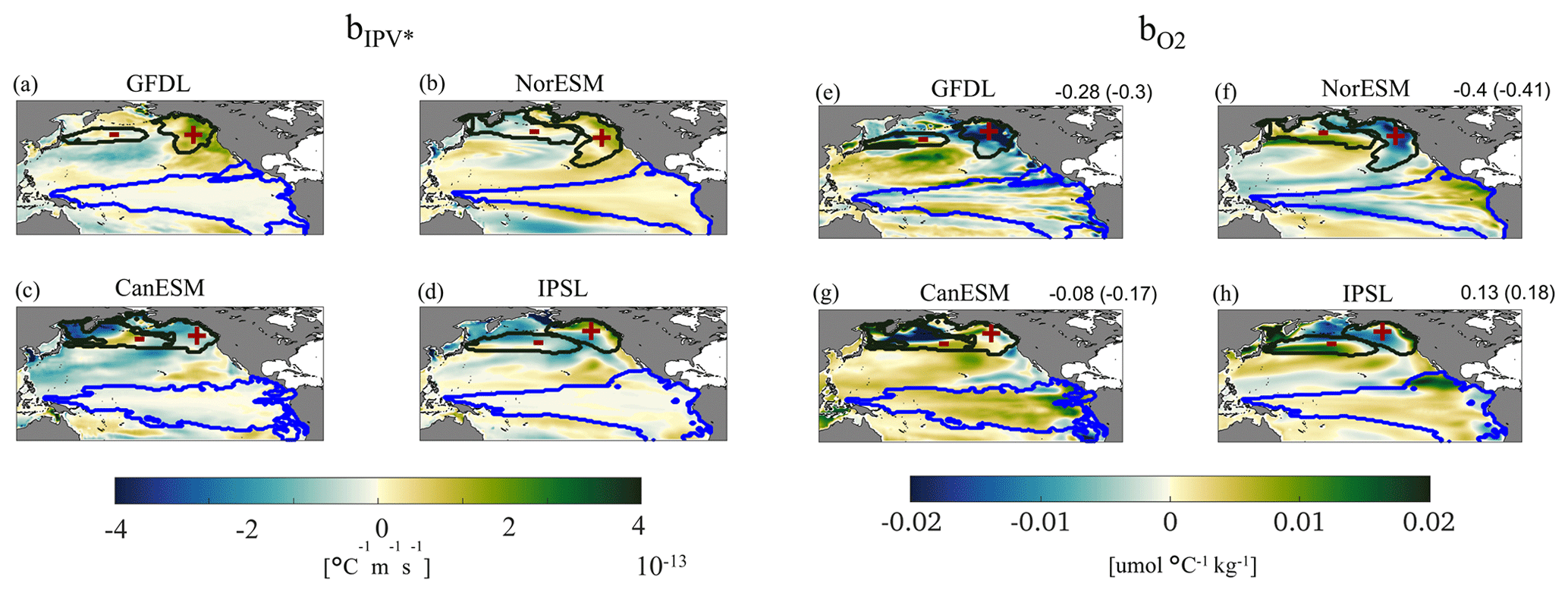
Figure 5 As in Fig. 4 but for the future projections. Color limits are fixed as ±3 standard deviations of the ensemble for each variable over the whole area ($\pm \mathrm{4.1}\times {\mathrm{10}}^{-\mathrm{13}}$ for IPV^* and ±0.02 for O₂). Values in parentheses are correlation coefficients (c.c.'s) computed north of 20° N. All c.c.'s passed a significance test at the 5 % level (see Supplement).

Overall, during the historical period, the residuals have an amplitude comparable to the PDO-forced signal (see Fig. S7), and the linear trends have similar patterns to but lower amplitude than the whole-field trends (see further discussion of trend shape when presenting Δ_means). In the future, on the other hand, linear trends of residuals and whole fields have similar patterns and intensities.

4.3 Hotspots of change (HYP 3)

As a last step, we evaluate changes in means, variability, and extremes for both variables (considering whole signals, i.e., not just the residuals) using the indicators introduced in “Materials and methods”. For the historical time frame, we divide the interval from 1950 to 2014 into two periods of equal length covering 1950 to 1981 and 1983 to 2014 (1960 to 1986 and 1988 to 2014 for E3SM-2G and ORAS4). We evaluated the indicators in each season separately or averaged together and found that differences across seasons were small, as measured by the standard deviation of the indicators (Figs. S10–S12). In the following we discuss only the indicators averaged across the four seasons without loss of information.

The representations of Δ_means in Fig. 6 show the changes in the mean fields, which have very similar patterns to the linear trend in both IPV^* and O₂ (see Fig. S7). By 2015, stratification has increased nearly everywhere in the ESMs, except for the equatorial upwelling region and the Kuroshio–Oyashio Extension. In ORAS4 there is also a prominent band in which stratification decreases between 10 and 20° N from the coast of the American continent to 150° W in the second period and in the overall trend. O₂ decreases in most of the North Pacific, especially in the subpolar gyre around the Kamchatka Peninsula, and increases in the upwelling areas along the coasts of Peru and Central America as well as in the California Current System. Regions of increasing O₂ are also found corresponding to the North Equatorial Current in the E3SM-2G hindcast and in the GFDL and CanESM models, in the equatorial upwelling band in NorEMS2, and in portions of the subpolar gyre around Alaska in E3SM-2G and IPSL.

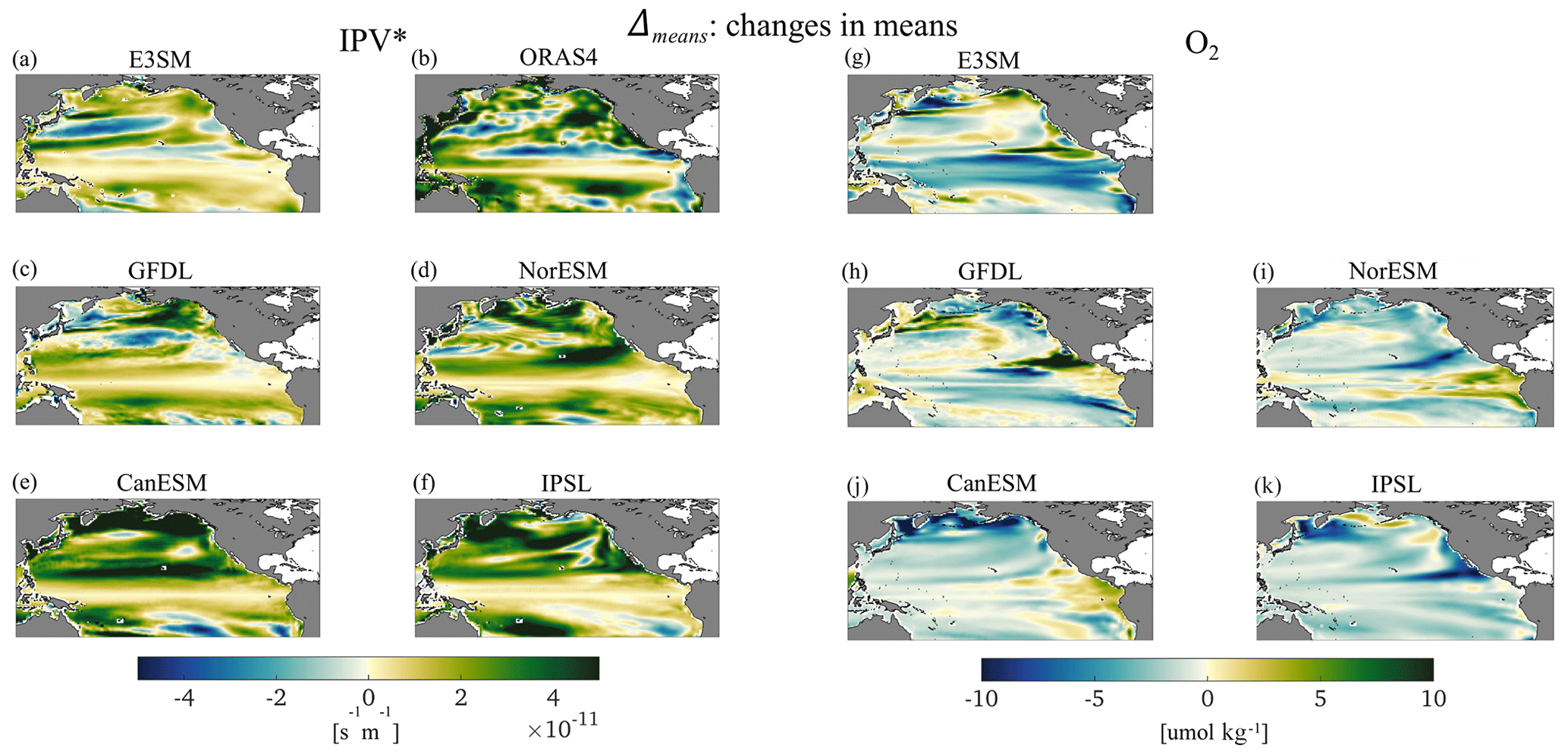
Figure 6 For the period from 1950 to 2014, Δ_means for IPV^* (left) and O₂ (right). All indicator maps are obtained by averaging the respective seasonal maps.

Indicators of change in (seasonal) variability (Δ_variability; Fig. 7) show strong differences across models in terms of patterns and, at least for O₂, intensity. Whenever corresponding maps of O₂ and stratification have the same sign and comparable amplitude at corresponding locations, they indicate that increments or decreases in IPV^* variability at seasonal scales are associated with corresponding increments in 0–200 m O₂ variability. In the hindcast, changes are greater for residual O₂ than for stratification. This is verified in three of the models in the northeastern extratropics. Among the models, GFDL and NorESM2 show patchy changes, both positive and negative, across the domain, with the smallest amplitudes among the datasets considered. CanESM undergoes predominately positive changes north of the Equator in IPV^* and negative changes to the south of it, while the variability in the O₂ field also decreases in the central portion of the subtropical gyre. In IPSL the variability increases nearly everywhere in both fields but especially at the Equator and to the south of it in IPV^* and more uniformly at all latitudes in O₂.

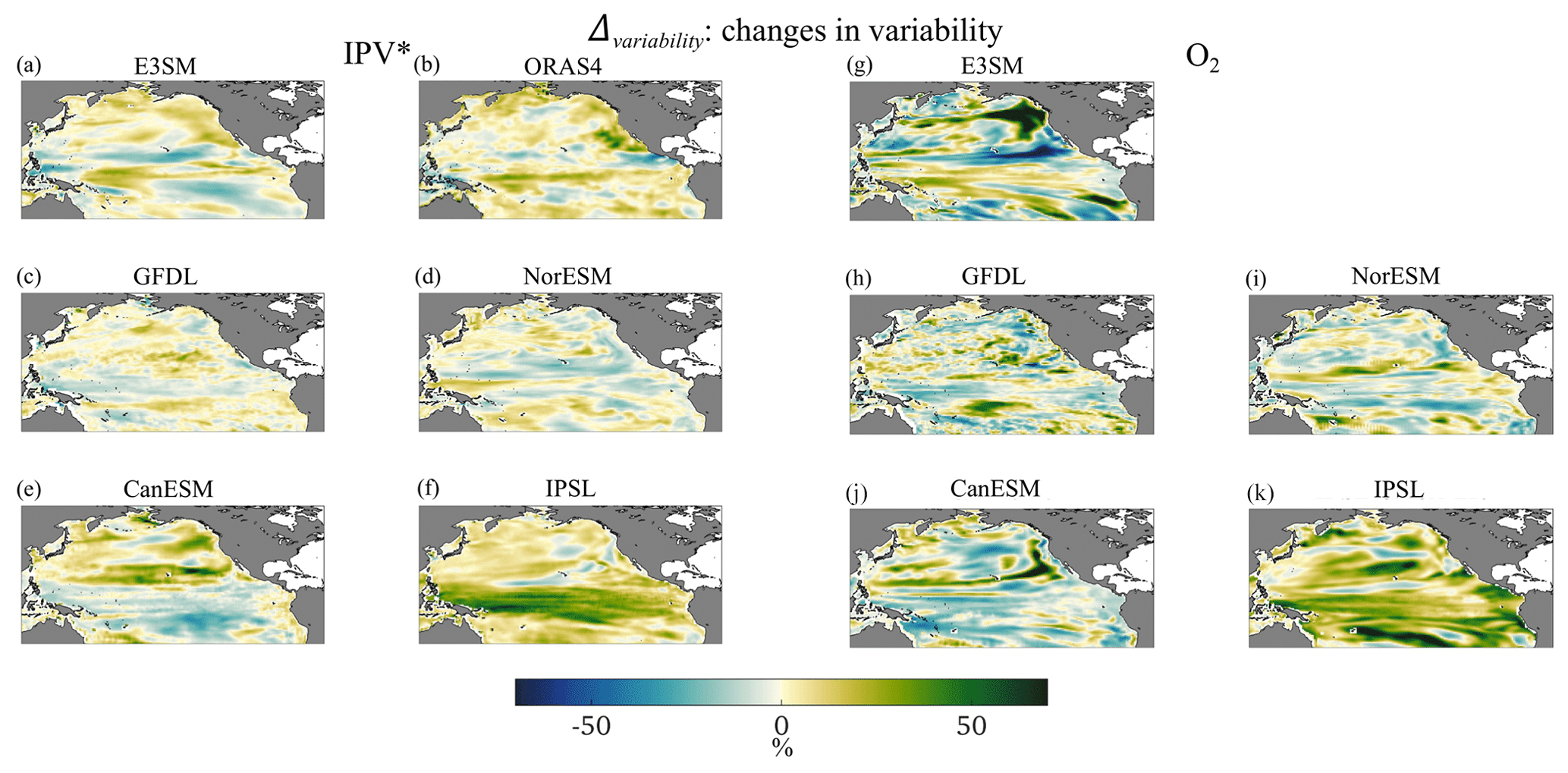
Figure 7 For the period from 1950 to 2014, Δ_variability for IPV^* (left) and O₂ (right).

Changes in extremes (Δ_extremes) for the O₂ field are stronger than for stratification (Fig. 8). Episodes of strong O₂ decrease and stratification increase are more frequent in period 2. For O₂ the regions to the north and south of the equatorial upwelling band emerge as most impacted in the E3SM-2G hindcast and GFDL, while the subtropical gyre displays an increase in extreme events nearly everywhere in CanESM and IPSL, at its boundary in E3SM-2G, and in its eastern portion in GFDL and NorESM. The subpolar gyre is affected especially in CanESM and IPSL. Changes in IPV^* extremes have less clear latitudinal differences and do not display a robust intensification at extratropical latitudes across the models. In ORAS4, maxima are found near the California Current System and in the warm-pool area.

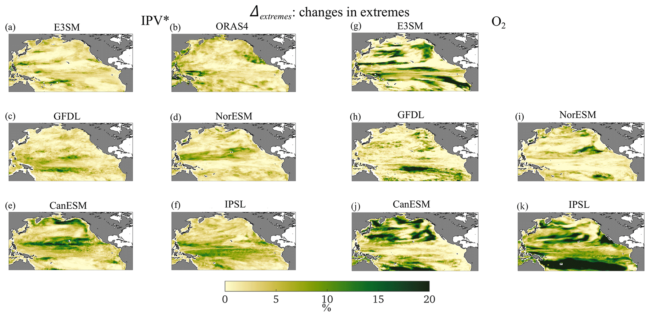
Figure 8 For the period from 1950 to 2014, Δ_extremes for IPV^* (left) and O₂ (right).

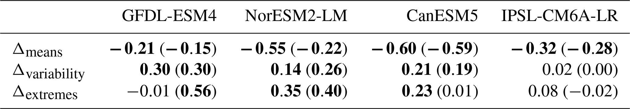
Table 2 Correlation coefficients (c.c.'s) for the period from 1950 to 2014 between the corresponding indicator maps for IPV^* and O₂. Bold values indicate a c.c. ≥ 0.1 that passed the shuffling significance test at the 5 % level (see Supplement). Numbers in parentheses reflect c.c.'s computed north of 20° N.

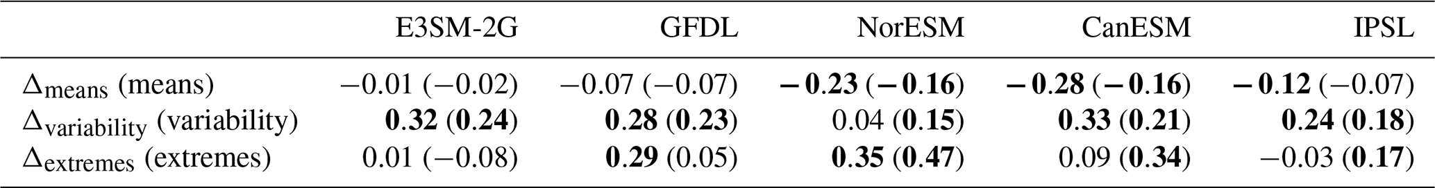
Table 2 summarizes the correlation coefficients between the maps of the three indicators for the two fields considered. Coefficients are negative for all models but small for Δ_means; slightly larger in amplitude and positive for the variability indicator (Δ_variability); and very small for Δ_extremes in the hindcast, CanESM, and IPSL analyses, while they are larger in amplitude and positive for GFDL, with a strong contribution from the equatorial region, especially in NorESM, where positive values are also found north of 20° N.

The resulting hotspot indices (SED), computed separately for the IPV^* and the O₂ indicators (see “Materials and methods”), are reported in Fig. 9. Except for IPSL, the hotspots are found outside the equatorial band. Those for O₂ are generally stronger along the eastern part of the subtropical gyres, in the eastern part of the PDO region, and along the California upwelling system, and the IPV^* hotspots are more commonly found over the western parts of the basin and along the southern boundary of the subtropical gyre. This result suggests a longitudinal decoupling between hotspots in O₂ and stratification in at least three of the models and in the hindcast, with NorESM being the exception due to the simulated superposition of the changes in extremes in the two fields. We also computed the SED for the residual fields, obtaining similar results (Fig. S13).

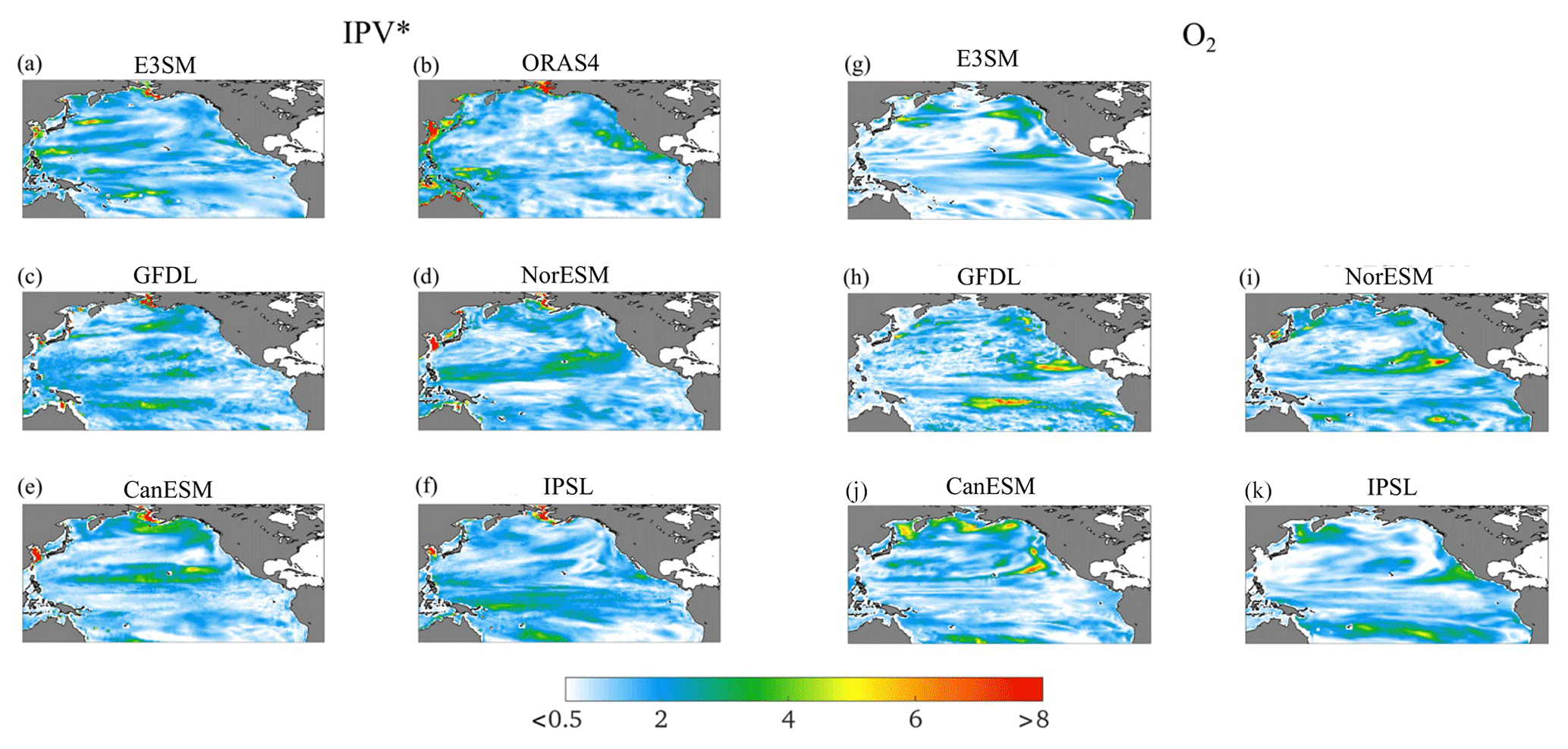
Figure 9 For the period from 1950 to 2014 (1960 to 2014 for E3SM-2G and ORAS4), SED index for IPV^* (left) and O₂ (right). The color scale is realized with rgbmap (Greene, 2023).

The maps of the indicators for the future projections follow in Figs. 10–12, again averaged over seasons, and the associated standard deviations are reported in Figs. S14–S16. In the projections, the seasonal differences are slightly greater compared to the historical period for Δ_means (IPV^*) in the northern subpolar gyres, especially for CanESM, NorESM, and IPSL (Fig. 10), and along the subtropical and the northern subpolar gyres for Δ_extremes(IPV^*) (Fig. 12). Standard deviations for Δ_extremes(O₂) are stronger along the extratropical gyres and weaker in the tropical upwelling region (Fig. S16). Areas of higher standard deviations in the projections are, however, associated with much stronger values of Δ_means and Δ_extremes compared to the historical period. In the projections, Δ_means strengthens significantly and is stronger than the actual trend shown in Fig. S9, indicating an acceleration of the changes in the last portion of the 21st century. This is especially relevant for IPV^* north of the Equator. Stratification increases everywhere except for regions in the Southern Hemisphere with different extension in the four models and mostly located in the central and eastern portions of the basin. O₂ decreases everywhere except for small areas around the equatorial upwelling band. The decrease is very strong along the northern boundary of the Pacific Ocean and, depending on the model, at the subtropical gyre boundary (NorESM and, to a lesser extent, CanESM) and south of the Equator along the coast of Central and South America (IPSL).

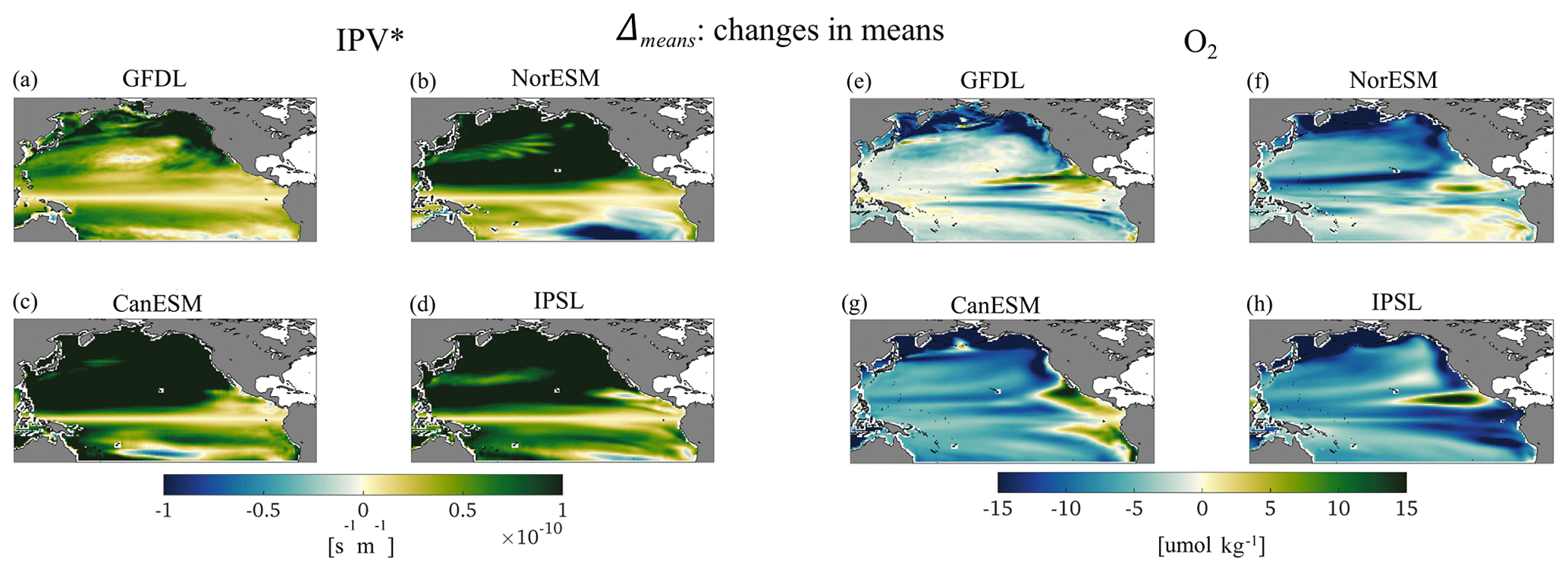
Figure 10 For the period from 2036 to 2100, Δ_means for IPV^* (left) and O₂ (right).

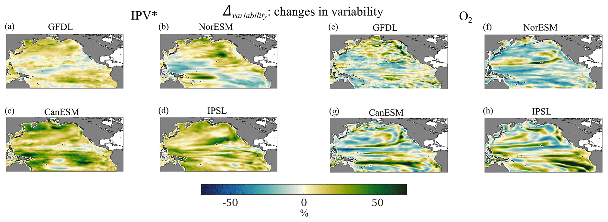
Figure 11 For the period from 2036 to 2100, Δ_variability for IPV^* (left) and O₂ (right).

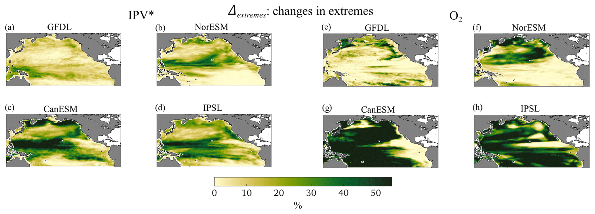
Figure 12 For the period from 2036 to 2100, Δ_extremes for IPV${}_{\mathrm{res}}^{*}$ (left) and residual O_2res (right). The percentage shown reaches 60 % (3 times higher than during the historical period; Fig. 8).

In terms of variability, when comparing the two variables, very few areas in Fig. 11 have a comparable sign and amplitude (which would indicate comparable increases or decreases). IPV^* variability increases in the warm pool and to the south of the Equator in the eastern portion of the basin in all models except for NorESM. O₂ variability increases in patchy areas mostly in the eastern half of the basin in GFDL, only along the southern boundary of the subtropical gyre in NorESM, roughly along the boundaries of the gyres in CanESM, and along the northern gyre boundary and south of the Equator in IPSL. Lastly, the extremes (Δ_extremes; Fig. 12) increase in CanESM and IPSL nearly everywhere except for the equatorial upwelling area for both variables, in NorESM in the Northern Hemisphere for O₂ and in the ENSO region for IPV^*, and in GFDL along the northern boundary of the basin for IPV^* and in the northern and southern portions of the domain for O₂. Correlations among maps of the two variables are generally very small for all indicators in the projections (Table 3), with $|\mathrm{c}.\mathrm{c}.|<\mathrm{0.4}$, except for Δ_means in NorESM and CanESM. Finally, we verified the robustness of our results to the choice of the ensemble member, computing the extreme indicators of four randomly chosen ensemble members of the CanESM model for the entire IPV^* and O₂ signals during the historical periods. We found no significant changes in extremes and SED (Figs. S17–S18).

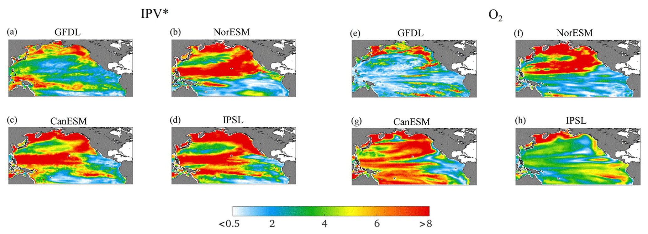
Figure 13 For the period from 2036 to 2100, SED index for IPV^* (left) and O₂ (right). The color scale was produced with rgbmap (Greene, 2023).

Table 3 The 2036–2100 correlation coefficients (c.c.'s) between the corresponding indicator maps for IPV^* and O₂. Bold values indicate c.c.'s ≥ 0.1 that passed the shuffling significance test at the 5 % level (see Supplement). Numbers in parentheses reflect c.c.'s computed north of 20° N.

5 Discussion and conclusions

State-of-the-art Earth system models (ESMs) can simulate many aspects of the Earth's observed climate and biogeochemical processes, thereby offering valuable insights into the future. Challenges persist, however, in reliably representing ocean biogeochemical dynamics (Schartau et al., 2017; Fennel et al., 2022). Biogeochemical processes can involve intricate interactions between multiple components of the Earth system (Pascal et al., 2024). These processes are often nonlinear, and couplings with physical climate processes are complex and challenging to interpret (e.g., Béal et al., 2010), thus requiring advances in diagnostic methods and interpretation. To assess model performance, continued efforts to develop metrics for model evaluation are needed. In this study we present new tools stemming from data-mining techniques that may contribute to this end. These quantitative approaches, together with advances in observation-based gridded products, can better characterize and extract information about linkages between physical and biogeochemical variables. In particular, biogeochemical data, including dissolved oxygen measurements, remain sparsely available compared to physical data. This limited availability of observational data hinders model validation. Exploiting linkages between the physical climate and oceanic O₂ can enhance the understanding and predictive skills of biogeochemical tracers. Examples of recently developed tools that take advantage of these linkages can be found in Giglio et al. (2018) and Sharp et al. (2023), who applied machine learning tools to the Argo-O₂ dataset to generate time-evolving maps of dissolved O₂ concentrations from seasonal to interannual timescales.

The overarching hypothesis in this work was that in the North Pacific, the spatiotemporal variability in O₂ reflects that of ocean ventilation (Talley et al., 2011), which can be measured by the magnitude of the isopycnic potential vorticity (IPV). A recent study (Ito et al., 2019) found that at subtropical latitudes, the variability in wintertime mixed-layer depths and the subduction of O₂ are linked to the PDO. Elevated O₂ levels emerge downstream of the deepened winter mixed layer during the positive phase of the PDO. According to the same study, in the equatorial Pacific, the variability in upper-ocean O₂ is linked to the stratification and the depth of the thermocline, which in turn are modulated by the PDO. A wide range of mechanisms have been suggested for the connection between upper-ocean O₂ and ventilation, many of which can be represented in ESMs. We should note, however, that Ito et al. (2019) also showed that extratropical O₂ variability involves multiple types of physical–biogeochemical coupling that may compensate one another. For example, ventilation variability (Ridder and England, 2014; Duteil et al., 2014; McKinley et al., 2004) can have the opposite imprint on O₂ than on water mass shifts, depending on the vertical stratification of temperature and O₂. In the subtropical thermocline, both temperature and O₂ decrease with depth, and vertical shifts of water masses generate positive correlations between them (Brandt et al., 2015; Duteil et al., 2014; Eddebbar et al., 2019). However, a negative relationship is expected between temperature and O₂ under ventilation-driven variability, as colder conditions are typically associated with stronger ventilation (and thus higher O₂). The superposition of these two processes may cause partial compensations and could amplify inter-model differences, especially in O₂ concentrations.

In this work, we tested the overarching hypothesis that the O₂ variability in the North Pacific is linked to that of ocean ventilation as measured by the magnitude of the isopycnic potential vorticity using four ESMs, a hindcast, and reanalysis data. We verified the simplistic view that the spatiotemporal variability in O₂ reflects that of ocean ventilation through the analysis of potential predictability, of the linkages between ventilation and O₂ with the dominant climate modes of the North Pacific, and of the patterns of extreme events in ventilation and O₂. As a tracer of physical ventilation, we chose isopycnic potential vorticity or IPV^*. Strong ventilation is assumed to generate a negative anomaly in IPV^*, which is then advected and mixed by physical circulation and mixing processes. Ventilation supplies O₂-rich surface waters into the interior ocean, implying a negative correlation between O₂ and IPV^*, as weak stratification (low IPV) may be linked to high oxygen. First, the information entropy (IE) was adopted to identify the areas in which IPV^* has a high predictability potential. Predictability was generally high along two stripes enclosing the ENSO pattern and excluding the upwelling cold tongue regions, which were found to correspond to areas in which O₂ and IPV^* are strongly anticorrelated. The underlying mechanisms are relatively well understood (Ito et al., 2019), and this behavior is robust across all the analyzed datasets and does not change significantly in the future projections of the four ESMs. Therefore, around the Pacific Equator, IPV^*, which is easily retrievable from temperature and salinity data, has a good predictability potential (higher than in the rest of the basin) and can be used as a proxy for O₂. The greater availability of temperature and salinity (and therefore stratification) observations from Argo floats, reanalyses, and modeled fields could be used in conjunction with the fewer co-located observations of O₂ to validate our findings and further extrapolate information about O₂ and its time evolution in these tropical areas.

Secondly, the variability in O₂ and IPV^* was examined in relation to large-scale modes of climate variability in the extratropical North Pacific. At mid-latitudes, the regional climate variability is PDO-dominated and our analysis shows very low predictability of IPV^*, unlike in the ENSO-dominated equatorial regions. The low predictability extends to the western boundary current and the Kuroshio–Oyashio Extension region. In the extratropical North Pacific, the (linear) contribution of the PDO to O₂ and IPV^* and the trends of their residuals have comparable amplitude over the historical period. This is not verified in the future projections, where the trends become increasingly dominant. Pattern correlations in the PDO regression maps (b coefficients) are generally quite small across the models.

Thirdly, we evaluated the hotspots of change in IPV^* and O₂ in the historical period and in the future projections. Overall, the historical hotspot indices or SED, computed separately for IPV^* and O₂, suggest a longitudinal decoupling across the two variables for all datasets except for one model, i.e., NorESM. In addition, most of the hotspots are in the extratropics. O₂ SEDs tend to be higher along the eastern portion of the basin, while IPV^* hotspots are mostly found over the western side of the basin and along the southern boundary of the subtropical gyre. The intensity of the SED increases over time from the historical period to the end of the 21st century. Larger changes and hotspots are found at the gyre boundaries and in the northern portion of the basin, from the Kamchatka Peninsula to the Gulf of Alaska. While O₂ loss is broadly linked to the strong increase in stratification, there are significant differences across model patterns, pointing to the need for further investigation.

The existing uncertainty in the CMIP6 models' representations of oxygen changes limits the information that can be extracted from the projections. We carried out our analysis on a sub-sample of the CMIP6 catalog only, but adding more models will not challenge this important conclusion. For a detailed model intercomparison of ocean deoxygenation in CMIP6 models, the reader is referred to Abe and Minobe (2023). Major sources of uncertainty in the future projections reside, for example, in their representation of the ENSO amplitude, as detailed in Beobide-Arsuaga et al. (2021), and in uncertainties regarding the amount of future warming (Tokarska et al., 2020) and, consequently, regarding the changes in upper-ocean stratification. Compared to the CMIP5 catalog, CMIP6 models tend to warm more and show a decline in subsurface oxygen ventilation with no consistent decrease in inter-model uncertainties (Kwiatkowski et al., 2020). Here we found that while in some models the relationship between IPV^* and O₂ becomes stronger, that is not the case for all models, and it is not verified in GFDL, which has the highest horizontal resolution and best compares to the reanalyses in the historical period.

A note of caution should be spent on the representation of regional changes and hotspots. The currently available spatial resolution for CMIP6 models does not resolve the fine-scale (mesoscale and finer) physical and biogeochemical processes occurring near the coast. This is especially true in regions of elevated nutrient supply such as along the California Current System and, more generally, in the eastern boundary upwelling systems (EBUS). Consequently, projected oxygen trends may exhibit variability even within subregions under the same scenario, as shown for EBUS by Bograd et al. (2023). However, analysis at the scales required to capture coastal dynamics would require higher-resolution models that would need – if projected into the future – boundary conditions from CMIP6 simulations. CMIP6 models indeed remain the primary tool for evaluating changes in large-scale modes of climate variability at interannual to decadal timescales. While resolution is an important limitation for coastal areas, our main findings remain relevant to the interpretation of the large-scale forcing. In particular the outcome of the hotspot analysis, i.e., that there is a large-scale longitudinal decoupling between the areas of most prominent changes in IPV^* and O₂ despite the PDO imprinting, is unlikely to be influenced by the models' resolution.

We found that the linkages between extratropical O₂ and PDO are model dependent and that the relationship is not as strong as hypothesized on the basis of the sparse available observations. In summary, the variability across the current generation of CMIP models is, for some of our hypotheses, too large to reach any definite conclusion regarding a signal which is weaker than expected. To alleviate this problem, we suggest using the new BGC-Argo array to validate the performance of each model by testing relationships between temperature, IPV, and O₂.

Models and reanalyses or hindcasts such as E3SM-2G allow for testing of whether there may be predictability, notwithstanding their biases and, for the case of the North Pacific, of whether there is a robust relationship across models between large-scale climate modes of variability, stratification, and O₂. The predictability potential extrapolated by global ESMs represents an upper bound of the actual one, but it is useful for identifying when further exploration may be warranted or where such an exercise may simply be futile. For example, the information entropy could be evaluated using opportunely interpolated Argo data (e.g., Smith and Murphy, 2007; Cheng and Zhu, 2016; and for BGC-Argo, Turner et al., 2023; Keppler et al., 2023; Sharp et al., 2023). In regions where the predictability potential is high, such an exercise is warranted; wherever the potential predictability is low, it would be futile. In reference to our second hypothesis, we found that the PDO modulates IPV^* and O₂ but that the signal is not robust across models, thus limiting the possibility of reconstructing the large-scale evolution of O₂ from temperature and salinity data alone. On the other hand, in the equatorial regions generally undersampled in historical O₂ datasets, the relatively high predictability of IPV^* and its strong link to O₂ could be exploited.

In summary, in this work we examined the relationship between the upper-ocean (0–200 m) oxygen (O₂) content and stratification in the North Pacific Ocean in four CMIP6 ESMs, an ocean hindcast simulation, and an ocean reanalysis. As far as the robustness of the relation between O₂ and IPV^* in the North Pacific is concerned (our first question), we found significant inter-model differences in the representation of climate variability in the North Pacific in CMIP6 models.

In relation to the linkages between O₂ and IPV^* compared to large-scale modes of climate variability such as PDO and ENSO (second question), we highlighted the potential of monitoring IPV^* to infer O₂ evolution in the ENSO area. However, we did not find a robust signal in terms of patterns and time evolution in the extratropics, where the PDO is the dominant mode of climate variability. The caveat is that the relationship, while weak, was nonetheless statistically significant under several metrics in the hindcast and in some models, of which GFDL-ESM4 is the best example.

Lastly, we found that the hotspots of changes in IPV^* and O₂ are not co-located (third and final question), which is especially true in the historical period.

In conclusion, the evolution trajectory of both stratification and oxygen in the North Pacific remains uncertain. Reducing this uncertainty would require monitoring IPV and O₂ simultaneously, for example through the accumulation of Argo floats equipped with CTD and O₂ sensors, to better quantify the large-scale co-variability in physical and biogeochemical parameters as a first step towards model improvement.