Global impact of benthic denitrification on marine N₂ fixation and primary production simulated by a variable-stoichiometry Earth system model

Nitrogen (N) is a crucial limiting nutrient for phytoplankton growth in the ocean. The main source of bioavailable N in the ocean is delivered by N₂-fixing diazotrophs in the surface layer. Since field observations of N₂ fixation are spatially and temporally sparse, the fundamental processes and mechanisms controlling N₂ fixation are not well understood and constrained. Here, we implement benthic denitrification in an Earth system model (ESM) of intermediate complexity (UVic ESCM 2.9) coupled to an optimality-based plankton–ecosystem model (OPEM v1.1). Benthic denitrification occurs mostly in coastal upwelling regions and on shallow continental shelves, and it is the largest N loss process in the global ocean. We calibrate our model against three different combinations of observed Chl, ${{\mathrm{NO}}_{\mathrm{3}}}^{-}$, ${{\mathrm{PO}}_{\mathrm{4}}}^{\mathrm{3}-}$, O₂, and $\mathrm{N}\text{*}={{\mathrm{NO}}_{\mathrm{3}}}^{-}-\mathrm{16}{{\mathrm{PO}}_{\mathrm{4}}}^{\mathrm{3}-}+\mathrm{2.9}$. The inclusion of N* provides a powerful constraint on biogeochemical model behavior. Our new model version including benthic denitrification simulates higher global rates of N₂ fixation with a more realistic distribution extending to higher latitudes that are supported by independent estimates based on geochemical data. The volume and water-column denitrification rates of the oxygen-deficient zone (ODZ) are reduced in the new version, indicating that including benthic denitrification may improve global biogeochemical models that commonly overestimate anoxic zones. With the improved representation of the ocean N cycle, our new model configuration also yields better global net primary production (NPP) when compared to the independent datasets not included in the calibration. Benthic denitrification plays an important role shaping N₂ fixation and NPP throughout the global ocean in our model, and it should be considered when evaluating and predicting their response to environmental change.

1 Introduction

Nitrogen (N) is a major limiting nutrient for phytoplankton growth throughout the majority of the tropical and subtropical oceans. N₂ fixation by photoautotrophic cyanobacteria supplies the ocean with most of its bioavailable N (Fig. 1). The main loss processes of fixed N are denitrification and anammox, which occur under low-oxygen conditions in the water column and sediment pore waters. In recent decades, numerous studies have been conducted to investigate water-column denitrification and anammox inside oxygen-deficient zones (ODZs). These studies have explored various aspects, including genomes, metabolism pathways and their rates, and microbial community structure, utilizing a range of modeling approaches (Hutchins and Capone, 2022). Research on benthic denitrification has been more limited, in spite of the greater part of global ocean denitrification (≈60 %–75 %) occurring in the sediments (Somes et al., 2013; DeVries et al., 2013; Eugster and Gruber, 2012; Brandes and Devol, 2002). Benthic denitrification is involved in N cycle stabilizing feedbacks over centennial timescales (Landolfi et al., 2017) and occurs primarily on continental shelves (Middelburg et al., 1996), where a high flux of particulate organic matter fuels the depletion of oxygen in sediment pore waters. Hence, this process is particularly susceptible to the impacts of human activities. Nevertheless, benthic denitrification is often not evaluated in the analysis of N₂ fixation (e.g., Bopp et al., 2022; Hamilton et al., 2020; Paulsen et al., 2017) or not included in current global biogeochemical models (e.g., Pahlow et al., 2020; Hajima et al., 2020; Dutkiewicz et al., 2015; Landolfi et al., 2013).

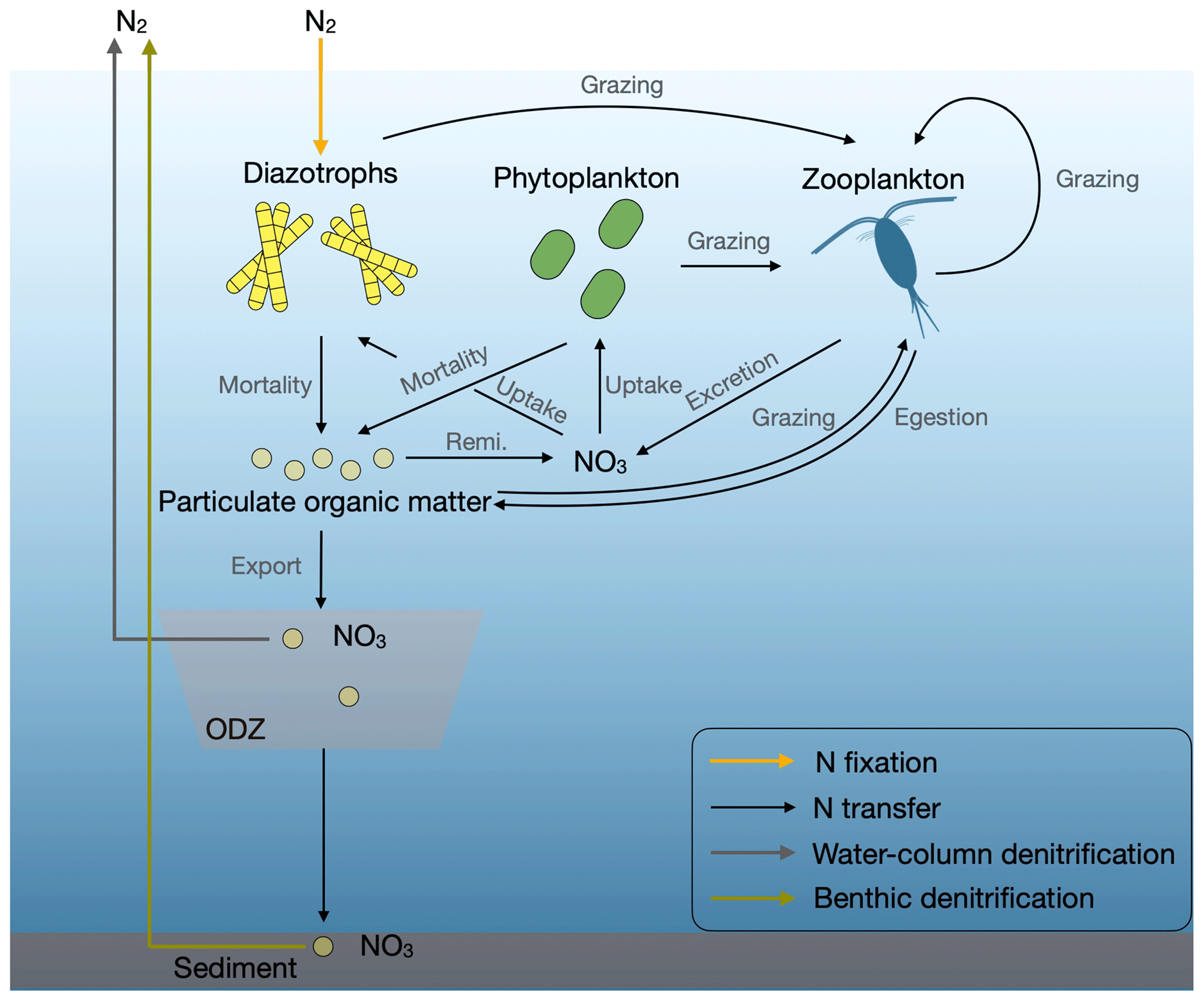
Figure 1 Marine N flows in our model. Remi. is remineralization, and ODZ is the oxygen-deficient zone.

In the marine nitrogen cycle, N loss processes convert bioavailable N to dinitrogen gas that creates an N deficiency compared to phosphate. With their activity, N₂ fixers replenish the nitrogen deficit in the surface ocean (Somes et al., 2013). Reproducing realistic patterns and rates of denitrification will thus be an important aspect for simulating N₂ fixation. In the ocean, a measure of the N deficit is generally expressed by the geochemical tracer N* (Gruber and Sarmiento, 1997), the deviation of nitrate relative to phosphate with respect to the Redfield N:P ratio (Redfield, 1934). Therefore, the distribution of N* has been used to infer rates of N₂ fixation and denitrification (e.g., Gruber and Sarmiento, 1997; Deutsch et al., 2007; Landolfi et al., 2008; Wang et al., 2019). We compare the ability of N* with that of ${{\mathrm{NO}}_{\mathrm{3}}}^{-}$ and ${{\mathrm{PO}}_{\mathrm{4}}}^{\mathrm{3}-}$ to constrain parameters of our prognostic model, which includes the representation of large-scale stoichiometric diversity of phytoplankton and diazotrophs (Pahlow et al., 2020).

Projections of how N₂ fixation evolves under global warming in current Earth system models (ESMs) are highly uncertain (Wrightson and Tagliabue, 2020). Since N₂ fixation can supply the N-limited surface waters with bioavailable nitrogen, it can have a strong impact on how net primary production (NPP) responds to climate change (Bopp et al., 2022; Landolfi et al., 2017). This suggests that a robust understanding of N₂ fixation and how it may respond to climate change is essential to predicting future changes in ocean NPP. The global impact of benthic denitrification on N₂ fixation and NPP is thus a major focus of this paper.

In this study, we implement an empirical parameterization for benthic denitrification (Bohlen et al., 2012) into a global ocean biogeochemical model with an explicit phytoplankton and diazotroph physiology (OPEM; Pahlow et al., 2020). We calibrate the model by conducting a large ensemble of simulations, whose parameter sets have been constructed via Latin hypercube sampling, and select the three best simulations according to an objective cost function based on different combinations of global observational datasets including N*. These simulations significantly improve not only the global N cycle, but also other important aspects of global marine biogeochemistry compared to the original OPEM without benthic denitrification. We explore model uncertainty by contrasting the behavior of our three optimized solutions. Finally, we discuss limitations and possible future developments.

2 Model description

We use the optimality-based plankton–ecosystem model (OPEM; Pahlow et al., 2020), which is incorporated into the UVic model version 2.9 (Weaver et al., 2001; Eby et al., 2009, 2013). Below we provide a brief description of the original OPEM implementation in UVic 2.9 (Pahlow et al., 2020), followed by the newly implemented benthic denitrification.

2.1 Physical configuration

The physical circulation configuration remains identical to previous UVic 2.9 Kiel versions (Pahlow et al., 2020; Nickelsen et al., 2015). The model has a horizontal resolution of 1.8° latitude × 3.6° longitude, and the ocean component has 19 levels in the vertical with thicknesses ranging from 50 m near the surface to 500 m in the deep ocean. The physical circulation model contains the zonally anisotropic isopycnal viscosity and diffusivity schemes to better reproduce equatorial undercurrents (Getzlaff and Dietze, 2013; Somes et al., 2010b). The atmospheric component consists of a simple 2D energy–moisture balance scheme with prescribed wind fields. The physical ocean model is forced by an observation-based monthly wind stress reconstruction (Kalnay et al., 1996). Atmospheric pCO₂ is prescribed and kept fixed at 284 ppm.

2.2 Optimality-based plankton–ecosystem model

The OPEM contains an optimality-based model (Pahlow et al., 2013) for non-N₂-fixing phytoplankton and diazotrophs with variable stoichiometry and an optimal current-feeding model (Pahlow and Prowe, 2010) with homeostatic stoichiometry and variable assimilation efficiency for the only zooplankton group. Phytoplankton and facultative diazotrophs allocate their resources optimally to maximize their net growth rates under different ambient environmental conditions. In contrast to the fixed-stoichiometry plankton–ecosystem implementation in UVic 2.9 (Keller et al., 2012), OPEM does not impose a priori a lower potential growth rate on diazotrophs than non-N₂-fixing phytoplankton, although the high cost of N₂ fixation (Pahlow et al., 2013) has a similar effect. OPEM also accounts for the variable stoichiometry of detritus and the associated remineralization. O₂ consumption for particulate organic matter decomposition is linked to contributions of C and N remineralization with respiratory quotients of $r_{-{\mathrm{O}}_{\mathrm{2}}:\mathrm{C}}=\mathrm{1.15}$ and $r_{-{\mathrm{O}}_{\mathrm{2}}:\mathrm{N}}=\mathrm{2}$, respectively.

The temperature dependence is from the OPEM-H configuration of Pahlow et al. (2020), which applies the Houlton et al. (2008) unimodal temperature function to N₂ fixation by diazotrophs. The growth and nutrient uptake of phytoplankton and diazotrophs follow the same exponential temperature function (Eppley, 1972). The temperature dependence in the OPEM configuration is the same as in the original UVic ESCM, where diazotrophs grow only when temperature is above 15 °C. Thus, the only difference between the OPEM and OPEM-H configurations is the temperature dependence of diazotrophs. Half-saturation iron concentrations of phytoplankton and diazotrophs are global constants and are calibrated as described in Sect. 2.4.

2.3 Benthic denitrification implementation

We include benthic denitrification as a transfer function, which has been empirically derived from benthic flux measurements (Bohlen et al., 2012). Denitrification scales linearly with the rain rate of particulate organic carbon (RRPOC) deposited on the seafloor and is amplified in environments with low oxygen and high nitrate levels. We apply the transfer function with the parameters obtained by Bohlen et al. (2012), which are the same as those implemented in Somes and Oschlies (2015) but differ slightly from the preliminary implementation in Somes et al. (2013). Anammox is implicitly accounted for in the denitrification estimate, since this parameterization is designed to capture total fixed-N loss (Bohlen et al., 2012; Koeve and Kähler, 2010) and our model does not differentiate between different species of dissolved inorganic nitrogen. We apply a sub-grid-scale bathymetry scheme where the effect of the unresolved high-resolution bathymetry is parameterized by multiplying by the area fraction of the seafloor in each grid cell (Somes et al., 2013; Somes and Oschlies, 2015). This is crucial for resolving high benthic denitrification rates over continental shelves smaller than the coarse-resolution model bathymetry.

2.4 Model calibration

2.4.1 Ensemble simulation setup

Our parameter settings are based on the OPEM-H configuration of Pahlow et al. (2020) and Chien et al. (2020). In order to allow a wider range of physiological differences between phytoplankton and diazotrophs, we increase the number of parameters to be calibrated by 5 from the pilot work. Thus, we vary 18 parameters in total (Table 1).

Table 1 Parameter names, ranges, units, and descriptions.

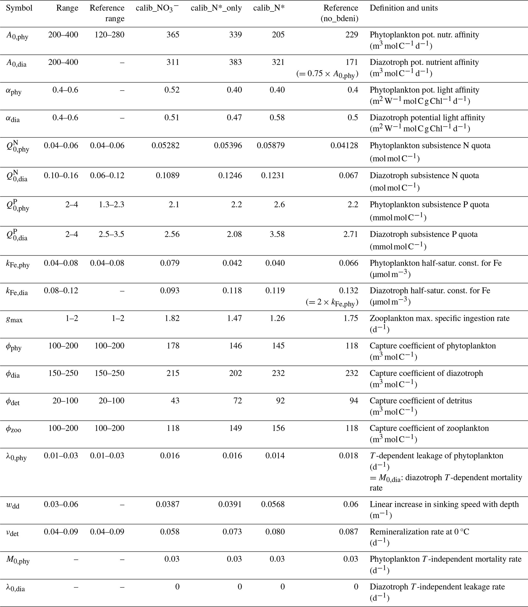
The reference range refers to the calibration range in Pahlow et al. (2020) and Chien et al. (2020). no_bdeni refers to OPEM_H in the previous studies (Pahlow et al., 2020; Chien et al., 2020).

The additional parameters are potential light affinity of phytoplankton (α_phy) and diazotrophs (α_dia), diazotroph half-saturation constant for Fe (k_Fe,dia), diazotroph potential nutrient affinity (A_0,dia), and linear increase in sinking speed with depth (w_dd). We allow diazotroph and phytoplankton parameters to vary independently, using the same ranges for phytoplankton and diazotrophs, and only impose the restriction $\mathrm{1}\le k_{\text{Fe,dia}}/k_{\text{Fe,phy}}\le \mathrm{3}$. This allows further decoupling of phytoplankton and diazotroph physiology compared to Chien et al. (2020) and Pahlow et al. (2020), who assumed that k_Fe,dia and A_0,dia co-vary with their phytoplankton equivalents. Additionally, we allow a 50 % overlap between the ranges of zooplankton grazing preference for diazotrophs and phytoplankton (Table 1) to enable a certain degree of freedom for these highly uncertain parameters.

The subsistence nutrient quotas ($Q_{\text{0, phy}}^{\mathrm{N}}$, $Q_{\text{0, phy}}^{\mathrm{P}}$, $Q_{\text{0, dia}}^{\mathrm{N}}$, and $Q_{\text{0, dia}}^{\mathrm{P}}$) are the minimum quotas for maintaining cellular integrity. The subsistence P quota range is the same for diazotrophs and phytoplankton, while the diazotrophs' subsistence N quota range is much higher than that of phytoplankton and also than the range used by Pahlow et al. (2020). This setting is more consistent with the earlier estimates (Pahlow et al., 2013) obtained by calibration with lab culture data for Trichodesmium (Holl and Montoya, 2008; Mulholland and Bernhardt, 2005).

We use the ranges of these parameters to generate a Latin hypercube ensemble of 600 different combinations of the 18 parameters selected for calibration. While the Latin hypercube method is efficient for evenly sampling a large-dimensional space, our 600 parameter sets provide only a very sparse coverage of this 18-dimensional parameter space, but we use this as a pragmatic choice to obtain information about suitable parameter regions.

Every ensemble member is spun up with pre-industrial (1850 CE) boundary conditions with fixed atmospheric pCO₂ of 284 ppm for 10 000 years. After the spin-up, we integrate for another year and use annual and monthly means of year 10 001 for model evaluation and analysis. Due to the simple atmospheric model that is driven by prescribed winds, the model has virtually no internal interannual variability, making this short analysis period a pragmatic choice.

2.4.2 Cost functions

To assess the model performance with respect to the spatial distributions of dissolved tracers and surface chlorophyll a, we apply global misfit metrics J based on a maximum-likelihood (ML) estimation method for parameters, assuming that the errors for the residuals of log-transformed variables between model simulations and observations follow normal distributions (Chien et al., 2020). Minimizing J ensures the best parameter estimates for the given model configuration.

Instead of calculating residuals between model simulations and observations for each model grid cell, we categorize model simulations and observations into 17 biomes (Fay and McKinley, 2014). Ocean biomes are geographical regions characterized by coherent large-scale patterns in physical and biogeochemical functions (Fay and McKinley, 2014), providing a representation of global ocean biogeography. We represent each variable by two statistical measures per biome: spatial average and variance. Therefore, the residuals comprise the discrepancies in spatial averages and variances for all biomes. In the vertical spatial dimension, we do not make any simplifications and residuals are calculated at each depth layer (k). We calculate the residuals of variables between monthly averaged simulations and observations to resolve seasonal variations in the upper ocean (0–550 m) and between annually averaged simulations and observations below 550 m.

Thus, the calculation of our cost function comprises two components for every depth level in our model:

$$\begin{array}{}\text{(1)}& J_k={\mathit{A}}_k^T{\mathbf{\Sigma }}_k^{-\mathrm{1}}{\mathit{A}}_k+{\mathit{V}}_k^T{\mathbf{Q}}_k^{-\mathrm{1}}{\mathit{V}}_k,k\in \mathit{\{}\mathrm{1},\mathrm{2},\mathrm{\dots },\mathrm{19}\mathit{\}},\end{array}$$

where A is the residual between the spatial means of observations (o) and the model (m), defined as $\mathit{A}=\text{mean}\left(\mathit{o}\right)-\text{mean}\left(\mathit{m}\right)$, and V is the residual in the spatial variance (var), defined as $\mathit{V}=\text{var}\left(\mathit{o}\right)-\text{var}\left(\mathit{m}\right)$. The covariance matrices of A and V are denoted by Σ and Q, respectively.

We apply the cost function to calibrate model solutions against three different combinations of types of observations. The first is identical to that employed by Chien et al. (2020), who chose four types of observations, i.e., nitrate, phosphate, and oxygen measurements from the World Ocean Atlas 2013 (WOA13) (Garcia et al., 2013a, b) and remote-sensing-derived surface chlorophyll concentration (NASA Goddard Space Flight Center et al., 2014). For the second, we use only $\text{N*}={{\mathrm{NO}}_{\mathrm{3}}}^{-}-\mathrm{16}\times {{\mathrm{PO}}_{\mathrm{4}}}^{\mathrm{3}-}+\mathrm{2.9}$ (Gruber and Sarmiento, 1997), which relates to several processes, including N₂ fixation and denitrification (e.g., Landolfi et al., 2008), to test the efficacy of N* for assessing model solutions. The third is the same as the first, except that we replace nitrate with N*. With these three calibrated solutions, we are able to characterize model uncertainty with respect to which observations are used for calibration.

3 Results and discussion

3.1 Ranges of global tracers and fluxes of the ensemble simulations

Within the 600 ensemble simulations, many tracer concentrations and fluxes span wide ranges (Fig. 2), except phosphate, because phosphorus is conserved in the model. Globally averaged ${{\mathrm{NO}}_{\mathrm{3}}}^{-}$ varies by a factor of 5 and N* varies from −23 to 12.5 mmol m⁻³ for the different parameter combinations. O₂ varies by a factor of 2, NPP varies by a factor of 4, globally integrated N₂ fixation rates vary by a factor of 10, benthic denitrification varies by a factor of 4, and water-column denitrification varies from 0 to 276 Tg N yr⁻¹. The differences between N₂ fixation and denitrification among all simulations range from −11.8 to 5 Tg N yr⁻¹, which indicates a slight imbalance at the end of the spin-up. The net fixed-N fluxes relative to N₂ fixation rates (N imbalance / N₂ fixation) range from −10 % to 4 % with a median of 0.3 %, in line with our steady-state assumption.

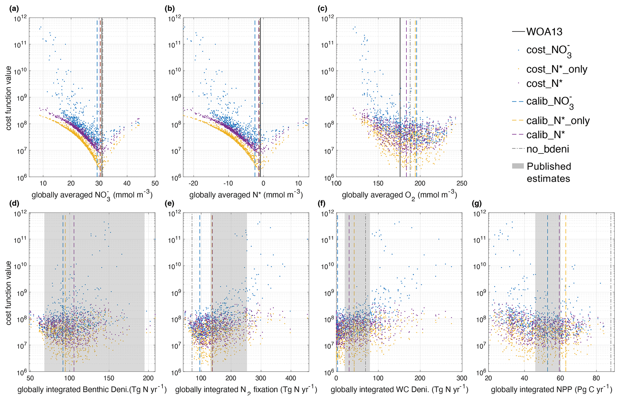
Figure 2 Relations between global averages of tracers, integral of fluxes, and cost function values. The x axis of each panel displays the ranges of (a) ${{\mathrm{NO}}_{\mathrm{3}}}^{-}$, (b) N*, (c) O₂, and (d) benthic denitrification; (e) N₂ fixation; (f) water-column denitrification; and (g) NPP of our ensemble simulations. The calibrated solutions are displayed as dashed lines with colors that correspond to their respective cost functions (cost_${{\mathrm{NO}}_{\mathrm{3}}}^{-}$, cost_N*_only, and cost_N*). In order to compare, we also depict the values of tracers from WOA13 data (Garcia et al., 2013a, b) with solid black lines and depict the tracers and fluxes from the simulation no_bdeni with dash-dotted gray lines. Deni. is short for denitrification, and WC is short for water column. Published estimates of global benthic denitrification, N₂ fixation, water-column denitrification, and NPP range from 68 to 195 Tg N yr⁻¹ (DeVries et al., 2013; Bohlen et al., 2012; Eugster and Gruber, 2012; Wang et al., 2019), from 131 to 253 Tg N yr⁻¹ (Großkopf et al., 2012; Luo et al., 2012; Landolfi et al., 2018; Shao et al., 2023), from 20 to 80 Tg N yr⁻¹ (Wang et al., 2019; DeVries et al., 2013; Somes et al., 2013; Bianchi et al., 2012; Eugster and Gruber, 2012), and from 46 to 60 Pg C yr⁻¹ (Johnson and Bif, 2021; Silsbe et al., 2016), respectively.

The different cost metrics yield similar optimal solutions (lowest cost function) for globally averaged ${{\mathrm{NO}}_{\mathrm{3}}}^{-}$, ${{\mathrm{PO}}_{\mathrm{4}}}^{\mathrm{3}-}$, N*, and O₂ (Fig. 2 and Table 1). The sharp gradients around the optimal solutions of global ${{\mathrm{NO}}_{\mathrm{3}}}^{-}$ and N* illustrate the strong constraints the cost function provides for these two tracers. In contrast to the original OPEM-H configuration (Fig. 4 in Chien et al., 2020), the majority of the globally averaged ${{\mathrm{NO}}_{\mathrm{3}}}^{-}$ simulations underestimate the observational average. Thus, our new model configuration with benthic denitrification has a stronger tendency to lose fixed N relative to original OPEM-H configuration without benthic denitrification, which one might expect from the incorporation of the additional N loss process.

3.2 Best model choice

We identify three optimal model solutions, calib_${\mathrm{NO}}_{\mathrm{3}}^{-}$, calib_N*_only, and calib_N*, based on the three cost functions that include different sets of observations and compare these with the OPEM-H configuration without benthic denitrification (no_bdeni) (Table 2 and Fig. 2) and observations (Fig. 2).

Table 2 Tracers, fluxes, and costs of OPEM simulations.

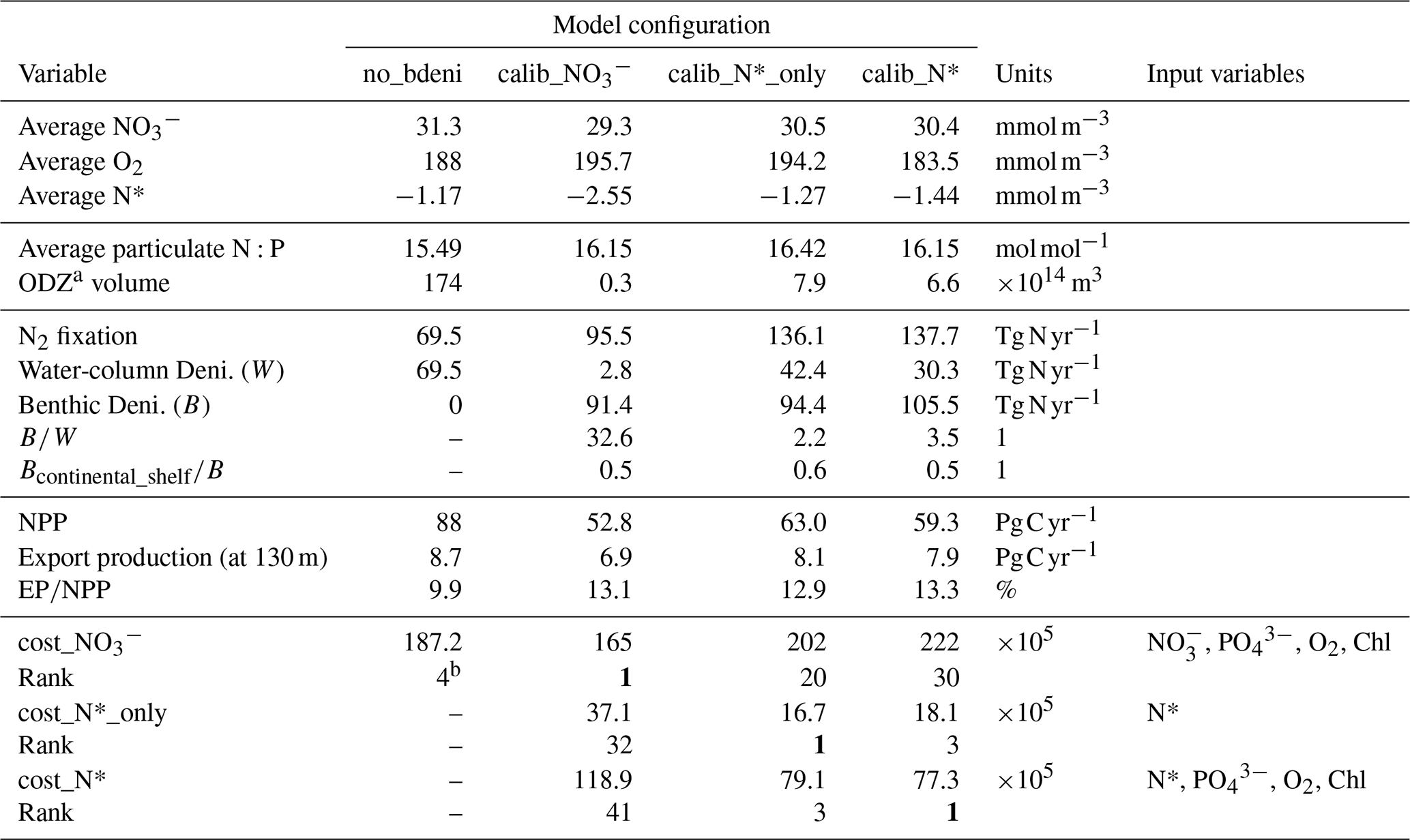
^a We define ODZ as the region with O₂ concentration <5 mmol m⁻³, and here we present the annual average of ODZ volume for each solution. ^b no_bdeni is the fourth-best solution among the 400 simulations conducted without benthic denitrification in the previous studies (Pahlow et al., 2020; Chien et al., 2020). All other rank numbers refer to the positions among the newly generated 600 simulations that incorporate benthic denitrification. cost_${{\mathrm{NO}}_{\mathrm{3}}}^{-}$ in this study is the same as the cost function in the previous studies.

Our solutions calib_N*_only and calib_N* appear better constrained than calib_${{\mathrm{NO}}_{\mathrm{3}}}^{-}$ (Fig. 2a–c). Globally averaged nitrate concentrations of calib_N*_only and calib_N* are closer to the WOA13 average of 31.0 mmol m⁻³ than calib_${\mathrm{NO}}_{\mathrm{3}}^{-}$, although calib_${{\mathrm{NO}}_{\mathrm{3}}}^{-}$ is calibrated directly against observed nitrate, whereas calib_N*_only and calib_N* consider nitrate only indirectly via N*. Globally averaged oxygen concentrations range from 183.5 to 195.7 mmol m⁻³, slightly above the observed WOA13 value of 176 mmol m⁻³. Interestingly, O₂ is also quite well constrained in calib_N*_only (Fig. 2c and Table 2), although it is calibrated only against N*.

While the inventory of nitrogen is essentially identical among the three optimal model solutions, the nitrogen fluxes vary widely. The calibrated estimates for water-column denitrification are more variable (2.8–69.5 Tg N yr⁻¹) than for benthic denitrification (91.4–105.5 Tg N yr⁻¹). This relatively weak constraint on water-column denitrification was also reported by Chien et al. (2020), who used an additional objective to constrain water-column denitrification to values above 60 Tg N yr⁻¹ (no_bdeni in Table 2). Correspondingly, the addition of benthic denitrification allows much higher estimates of global N₂ fixation than no_bdeni.

The high variability in water-column denitrification is much reduced in calib_N*_only and calib_N*, ranging from 30.3 to 42.4 Tg N yr⁻¹, hence varying similarly to our benthic denitrification estimates of 94.4–105.5 Tg N yr⁻¹. Thus, incorporating N* into the calibration objective helps reduce the uncertainty of ocean nitrogen fluxes, particularly water-column denitrification. Moreover, using N* also yields more reasonable rates of water-column denitrification and global N₂ fixation. Globally integrated water-column denitrification has been estimated between 39–77 Tg N yr⁻¹ (Eugster and Gruber, 2012; DeVries et al., 2012, 2013; Somes et al., 2013; Wang et al., 2019). This suggests that N* provides a better, more independent constraint on water-column denitrification rates, and hence on N₂ fixation, than simply combining ${{\mathrm{NO}}_{\mathrm{3}}}^{-}$ and ${{\mathrm{PO}}_{\mathrm{4}}}^{\mathrm{3}-}$. ${{\mathrm{NO}}_{\mathrm{3}}}^{-}$ and ${{\mathrm{PO}}_{\mathrm{4}}}^{\mathrm{3}-}$ are highly correlated, largely following the Redfield N:P ratio. The correlations between different data (Chl, ${{\mathrm{NO}}_{\mathrm{3}}}^{-}$, ${{\mathrm{PO}}_{\mathrm{4}}}^{\mathrm{3}-}$, and O₂) are already accounted for by our misfit metric (Krishna et al., 2019). However, N* not only accounts for the correlation between ${{\mathrm{NO}}_{\mathrm{3}}}^{-}$ and ${{\mathrm{PO}}_{\mathrm{4}}}^{\mathrm{3}-}$, but it can be related directly to non-Redfield processes, such as N₂ fixation, denitrification, and variations in particulate $\mathrm{C}:\mathrm{N}:\mathrm{P}$ stoichiometry.

With the representation of benthic denitrification in our model and the inclusion of N* into our cost function, global N₂ fixation rates are between 136.1–137.7 Tg N yr⁻¹, which is close to previous estimates of 137 Tg N yr⁻¹ (Deutsch et al., 2007) and 163 Tg N yr⁻¹ (Wang et al., 2019). Our estimates also fall within the range of extrapolations of direct measurements, which yield marine N₂ fixation rates between 131 and 253 Tg N yr⁻¹ (Großkopf et al., 2012; Luo et al., 2012; Landolfi et al., 2018; Shao et al., 2023).

Globally integrated net primary production (NPP) rates among our three calibrated simulations are consistently lower than those of no_bdeni (88 Pg C yr⁻¹), from 52.8 to 63.0 Pg C yr⁻¹. This is much closer to observation-based estimates of 52 (satellite-based; Silsbe et al., 2016) and 53 Pg C yr⁻¹ (derived from Argo oxygen measurements; Johnson and Bif, 2021). Export production (EP) at 130 m (model euphotic depth) ranges from 6.9 to 8.1 Pg C yr⁻¹, slightly lower than that of no_bdeni (8.7 Pg C yr⁻¹; Table 2), yielding higher export efficiencies (export production$/$NPP) than no_bdeni. Approximately 13 % of NPP is exported as sinking particles to the deep ocean in our new solutions (Table 2). Simulated export production at 100 m in the Coupled Model Intercomparison Project Phase 5 (CMIP5) and newer CMIP6 models ranges from about 4.5 to 7.5 Pg C yr⁻¹ (Bopp et al., 2013; Laufkötter et al., 2016; Fu et al., 2016) and 5 to 12 Pg C yr⁻¹ (Séférian et al., 2020; Henson et al., 2022), respectively. Thus, our estimates fall within the CMIP6 spread. Other data-assimilated global ecosystem and biogeochemistry models yield particulate organic carbon export across the 100 m depth horizon of 10.64 (Wang et al., 2023), 6.4 (Nowicki et al., 2022), and 6.7 Pg C yr⁻¹ (DeVries and Weber, 2017), yielding export ratios between 12 % and 20 %.

Considering the constraints of oxygen, NPP (Fig. 2c and g), and particulate N:P (Table 2), our best solution is calib_N*, which is calibrated by the cost function cost_N*.

3.3 Global patterns of N fluxes

3.3.1 Overview of benthic denitrification

Due to the similarity of global benthic denitrification patterns and rates in our calibrated solutions, we show the mean of benthic denitrification from three calibrated solutions (Figs. 3 and 4j–l). Benthic denitrification rates are highest in highly productive regions over shallow continental shelves (e.g., South and East China Seas, Bering Sea) (Fig. 3a). These areas experience benthic denitrification rates over 100 times greater than deep-ocean sediments.

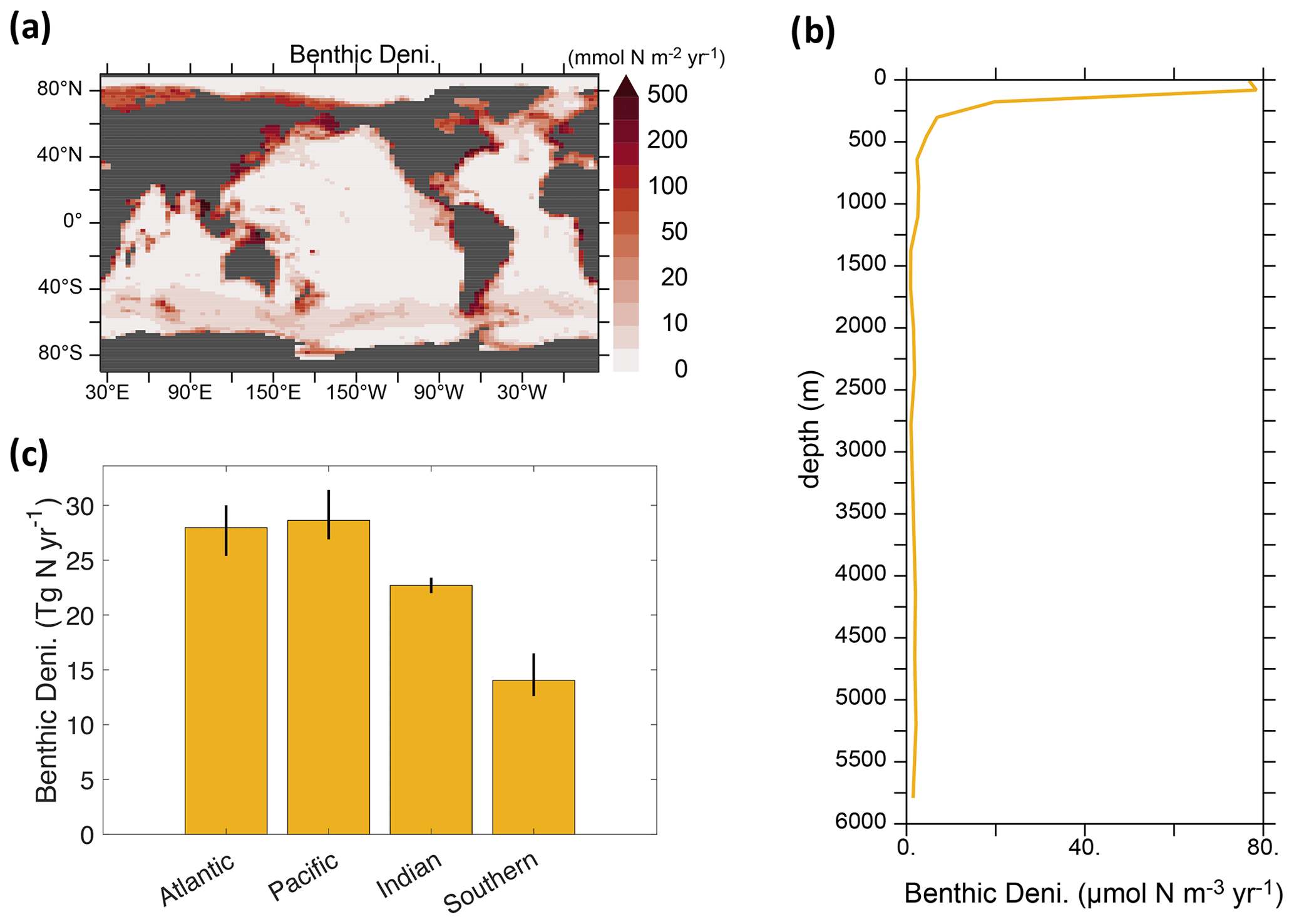
Figure 3 Spatial distributions of benthic denitrification, based on the mean values obtained from our calibrated solutions. (a) Geographic distribution of the vertical integrals. (b) Vertical profile of the global averages. (c) Four ocean basin integrals. The Southern Ocean is defined as the body of water located south of 40° S. The error bar in panel (c) indicates the uncertainty window among the calibrated solutions (i.e., calib_${{\mathrm{NO}}_{\mathrm{3}}}^{-}$, calib_N*_only, and calib_N*).

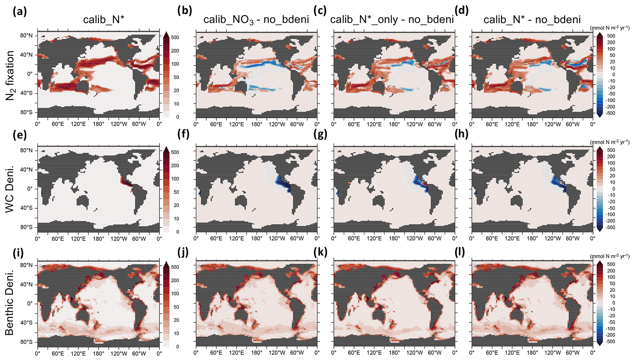
Figure 4 N₂ fixation, water-column denitrification, and benthic denitrification distributions of calib_N* and the changes in three new solutions relative to no_bdeni.

The vertical profile of globally integrated benthic denitrification experiences a sharp increase in the upper ocean, with the highest rates on shallow continental shelves (<160 m depth) (Fig. 3b), accounting for approximately 50 % of the total benthic denitrification (Table 2). It should be noted that benthic denitrification is not confined to the upper ocean but occurs at all depths. This is in contrast to water-column denitrification, which typically occurs in the upper 900 m where oxygen-deficient zones develop, and to N₂ fixation, which is confined to the euphotic upper 130 m in our model (Fig. A1). The average of the calibrated solutions predicts the largest contributions from sediments in the Pacific and Atlantic oceans (Fig. 3c).

3.3.2 Influence of benthic denitrification on other N fluxes

The global oceanic fixed-N inventory is maintained by a balanced supply of N by N₂ fixation at the surface ocean and removal by water-column and benthic denitrification. Figure 4 depicts the global N fluxes of our best model solution calib_N* and the flux changes relative to no_bdeni for each of the three solutions. With the implementation of benthic denitrification, global N₂ fixation increases, shifting polewards in the Pacific and intensifying in the Atlantic and southern Indian oceans relative to no_bdeni. The increased N₂ fixation thereby compensates for the extra N loss due to benthic denitrification in our newly calibrated simulations. With the outward extension of N₂ fixation, however, mild decreases relative to no_bdeni occur in the centers of the subtropical gyres of the Atlantic and Pacific oceans.

Water-column denitrification declines relative to no_bdeni (Table 2). The two new simulations calib_N*_only and calib_N* show very similar changes, with generally strong decreases in the volume of the eastern tropical North Pacific oxygen-deficient zone (ODZ) (Fig. 4g and h). Our model does not reproduce the ODZ in the Indian Ocean, hence the absence of water-column denitrification there. This is also the main reason for the very low rates of N₂ fixation predicted for the northern Indian Ocean, which could be unrealistic. However, there is considerable uncertainty about the regional pattern of N₂ fixation in the northern Indian Ocean due to the sparsity of available observations. For example, Shao et al. (2023) found strong N₂ fixation rates in only a few places along the southwestern coast of India in the eastern Arabian Sea, Löscher et al. (2020) could find no evidence for N₂ fixation in the Bay of Bengal, and vast areas in the northern and western Indian Ocean remain unsampled. Aligned with the lowest global integrated flux of water-column denitrification of calib_${\mathrm{NO}}_{\mathrm{3}}^{-}$, water-column denitrification rates are reduced almost everywhere.

We calculate the basin-scale N fluxes shown in Fig. 5 and Table A1. The net fixed-N flux is negative in the Pacific Ocean and positive in the Atlantic Ocean. The Atlantic remains the primary N source for the global ocean, as does no_bdeni. This is mainly caused by the relatively strong iron limitation on diazotrophs in the Pacific Ocean that prevents them balancing the high denitrification rates there, which is alleviated in the North Atlantic Ocean, where there is high atmospheric iron input from Saharan dust (Somes et al., 2010a; Landolfi et al., 2013; Weber and Deutsch, 2014). The very low N₂ fixation rates in the South Pacific (Fig. 4a) can be attributed to the underestimated surface dissolved iron concentration in this region. Since our solutions lack water-column denitrification in the Indian Ocean, this area supplies extra nitrogen to the global ocean, even when benthic denitrification is taken into account. In contrast, the Southern Ocean (SO) becomes a nitrogen sink when benthic denitrification is included, as N₂ fixation does not occur in this area.

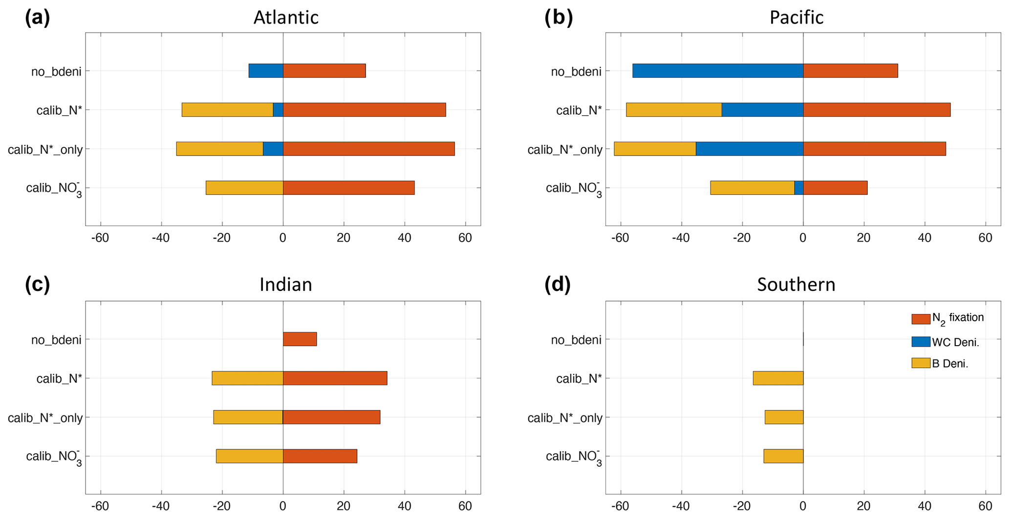
Figure 5 Basin-scale bioavailable N fluxes in the Atlantic (a), Pacific (b), Indian (c), and Southern (d) oceans, including N₂ fixation, water-column denitrification, and benthic denitrification.

3.4 Spatial distributions of biogeochemical tracers

3.4.1 Vertical nutrient distributions

We now compare the vertical distributions of nutrients and oxygen in our newly calibrated simulations to those in the WOA13 (Garcia et al., 2013a, b) and no_bdeni, as global averages and for individual ocean basins (Fig. 6). All simulations reproduce the major patterns of the observed climatological vertical distributions of ${{\mathrm{NO}}_{\mathrm{3}}}^{-}$ and ${{\mathrm{PO}}_{\mathrm{4}}}^{\mathrm{3}-}$, although N* profiles deviate the most from the WOA13 average. This is due to the smaller range of N* (−4.5–2.5 mmol m⁻³; Fig. 6c) compared to that of ${{\mathrm{NO}}_{\mathrm{3}}}^{-}$ (0–40 mmol m⁻³; Fig. 6a) and $\mathrm{16}\times {{\mathrm{PO}}_{\mathrm{4}}}^{\mathrm{3}-}$ (0–48 mmol m⁻³; Fig. 6b). The simulation no_bdeni underestimates N* in the upper 1000 m, whereas the simulations the include benthic denitrification and are calibrated to N* (i.e., calib_N*_only and calib_N*) better reproduce upper-ocean N* where N cycle fluxes are strongest. In the deep ocean (below 1000 m), due to the addition of benthic denitrification, both calib_N*_only and calib_N* depart more from the observation than no_bdeni, especially in the Pacific and Southern oceans, suggesting that benthic denitrification is overestimated there. The greatest deviation in the N* profiles, particularly in the deep ocean, occurs in calib_${\mathrm{NO}}_{\mathrm{3}}^{-}$.

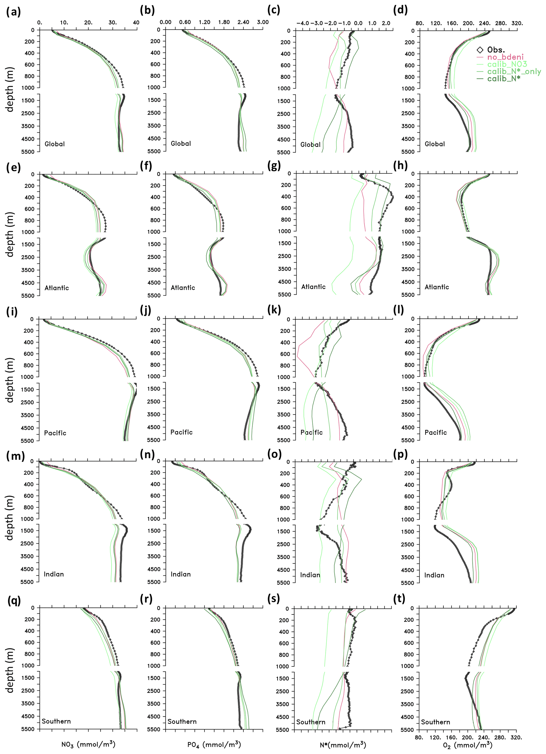
Figure 6 Vertical distributions of tracers (${{\mathrm{NO}}_{\mathrm{3}}}^{-}$, ${{\mathrm{PO}}_{\mathrm{4}}}^{\mathrm{3}-}$, N*, and O₂) in the global ocean and in the Atlantic, Pacific, Indian, and Southern oceans.

Profiles of N* result from the vertical distributions of the processes affecting N* and from the impact of ocean circulation. Denitrification occurs both in the water column and in the sediments and imparts a negative signature to N*, whereas N₂ fixation imparts a positive signature to N* in the upper ocean. Our calibrated solutions with benthic denitrification yield higher N₂ fixation in the euphotic zone and lower water-column denitrification in oxygen-deficient zones (ODZs) compared to no_bdeni, both of which contribute to increasing upper-ocean N* compared to no_bdeni, thereby better reproducing observed N* profiles. However, benthic denitrification also occurs at high rates in the upper ocean on the continental shelves, which can compensate the N* effects of N₂ fixation and lead to reduced N* relative to no_bdeni in the shallow subsurface ocean (e.g., calib_N*_only in the Atlantic and Indian oceans). The low vertical N* variability in the Indian Ocean from 200 to 1000 m is due to the lack of an ODZ and subsequent water-column denitrification. This is partially counteracted by high benthic denitrification in the upper 200 m, causing an upper-ocean N* gradient inconsistent with observations. In order to disentangle the individual effects, we also show the horizontal distribution of N*, which will be addressed in Sect. 3.4.2.

For O₂, all model simulations slightly overestimate global-averaged deep-ocean O₂, although the vertical patterns are generally consistent with observations. The positive bias in the Southern Ocean (SO) occurs in intermediate layers (300–2500 m). Indian Ocean Deep Water (IODW; 1400–3500 m) deviations relative to observations have been partly attributed to the overestimation of O₂ in the SO (Schmidt et al., 2021), as Circumpolar Deep Water (CDW) is the origin of IODW.

Global O₂ profiles of our new simulations show increased concentrations relative to no_bdeni in the mesopelagic zone (200–1000 m), where the distribution of O₂ is largely dominated by the remineralization of particulate organic matter (POM). This is likely caused by the slightly decreased global export production described above (Table 2). O₂ concentrations in the upper 1000 m are lower in calib_N* and calib_N*_only than in calib_${\mathrm{NO}}_{\mathrm{3}}^{-}$. This may be explained by the higher calibrated remineralization rates (ν_det) when the model is constrained with N* (either calib_N* or calib_N*_only) compared to when it is constrained with ${{\mathrm{NO}}_{\mathrm{3}}}^{-}$ (Table 1). Notably, the vertical O₂ profiles of calib_N*_only are in close proximity to the observations, implying that N* alone sufficiently constrains the distribution of O₂ in our model. As both water-column and benthic denitrification are tightly linked to oxygen, a proper representation of the N* distribution requires a realistic reproduction of the oxygen distribution in the model that resolves major marine biogeochemical processes properly.

3.4.2 Lateral distribution of N*

Examining the horizontal distribution of N* at the surface allows us to disentangle the local and regional responses of N* to N₂ fixation and benthic denitrification. The inclusion of benthic denitrification considerably improves the reproduction of observed near-surface (50 m) N* in the North Pacific subpolar gyre (Fig. 7c), which is largely occupied by shallow continental shelves extending into the Okhotsk and Bering Seas (Fig. 3a). Likewise, near-surface N* in the Arctic Ocean is lower than in no_bdeni, more in line with the observations (Fig. 7a–c). Here, however, this improvement is limited, likely due to the coarse resolution. Our model lacks the representation of narrow continental shelves (e.g., among the Canadian Arctic Archipelago) and the circulation around them.

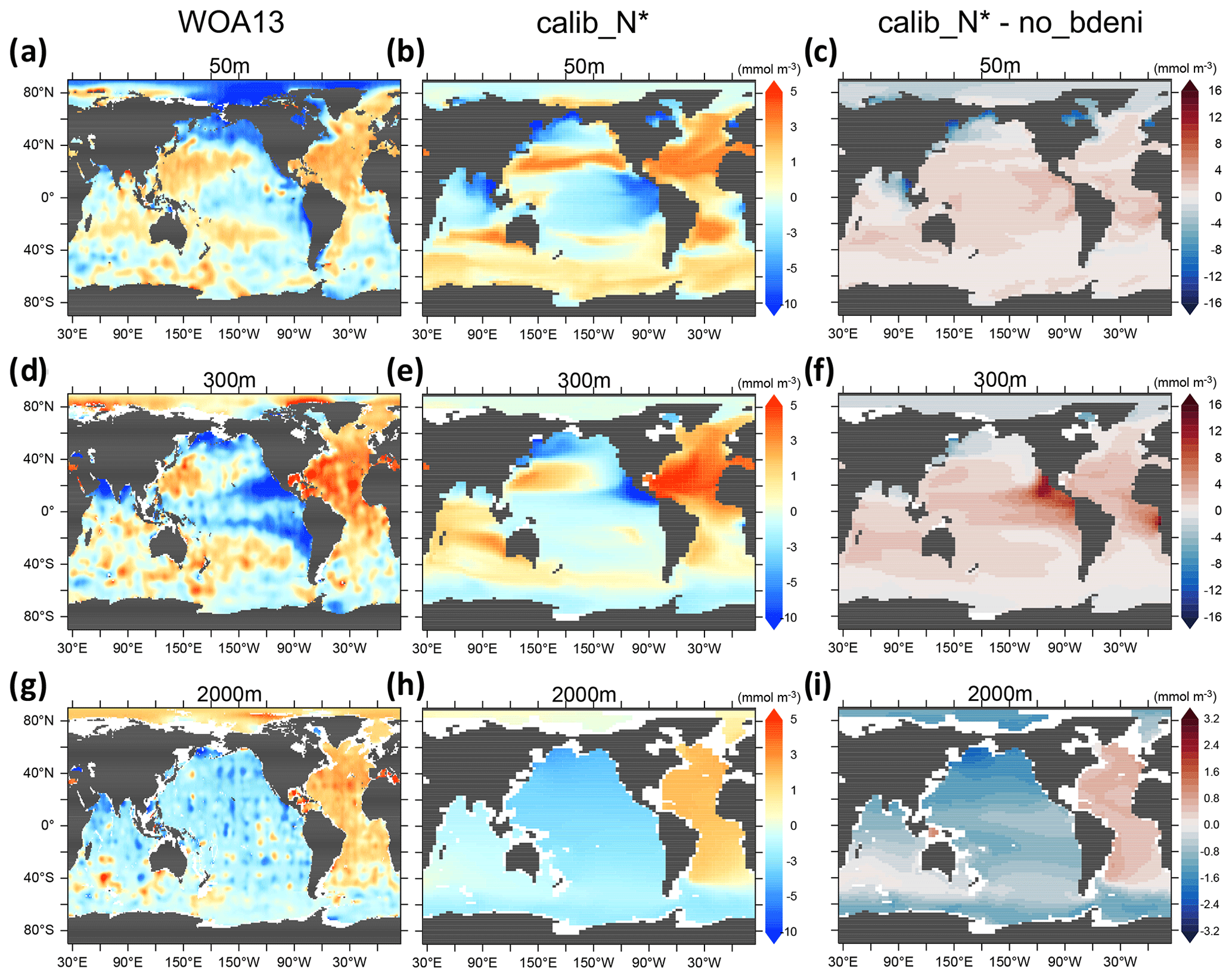
Figure 7 Spatial distribution of N* (50, 300, and 2000 m) for WOA13 and one of our calibrated solutions, calib_N*, along with changes in this calibrated solution compared to no_bdeni.

The twilight zone collects euphotic zone signals through the sinking and remineralization of organic matter. Thus, the non-Redfield stoichiometry of the exported organic matter, local denitrification in both the water column and the sediments, and N₂ fixation all contribute to the horizontal pattern of N* at 300 m. The low N* signal originating from excessive water-column denitrification at 300 m in no_bdeni is mitigated in the eastern tropical North Pacific ODZ and is nearly gone in the eastern tropical South Pacific ODZ in the new simulations (Fig. 4). The optimal model solutions better simulate elevated N* in the Atlantic Ocean, Indian Ocean, and western North Pacific (e.g., see calib_N* in Fig. 7f). This is due to the higher contribution of N₂ fixation in these regions (Fig. 4) relative to no_bdeni, but it is also due to the elevated euphotic phytoplankton and associated detritus N:P (not shown) with the assumption of identical remineralization rates of detrital N and P. Compared to the observations, our model underestimates N* in the western and central parts of the South Pacific subtropical gyre. This signal is driven both by underestimated N₂ fixation rates (Fig. 4a) and by low N:P ratios of phytoplankton and corresponding detritus N:P (<13.5) compared to the Redfield ratio (molar $\mathrm{N}:\mathrm{P}=\mathrm{16}$) that is applied in the calculation of N*.

The influence of local biogeochemical processes on N*, such as benthic denitrification, is scarcely discernible at 2000 m. The distribution of N* in the deep ocean reflects global biogeochemical signals accumulating over decades to millennia along the thermohaline circulation (Fripiat et al., 2021; DeVries and Primeau, 2011), thus diluting the local flux signals. Our simulations constrained by N* (calib_N*_only and calib_N*) best reproduce the basin gradient visible in the WOA13 data (see calib_N* in Fig. 7h).

3.4.3 Patterns of O₂

In the core of the ODZs (≈300 m), the O₂ distribution varies similarly across all calibrated new simulations compared to no_bdeni (not shown). Low- and mid-latitude oceans have higher subsurface oxygen concentrations (Fig. 8), resulting in less intense ODZs and water-column denitrification (Fig. 4). The simulated and observed spatial patterns are broadly comparable, with the exception of the Arabian Sea, where the observations reveal the presence of a perennial ODZ (Fig. 8a). The lower ODZ volume when including benthic denitrification (Table 2) implies that including benthic denitrification may improve the representation of ODZs in global ocean biogeochemical models that typically overestimate their volume (Cabré et al., 2015).

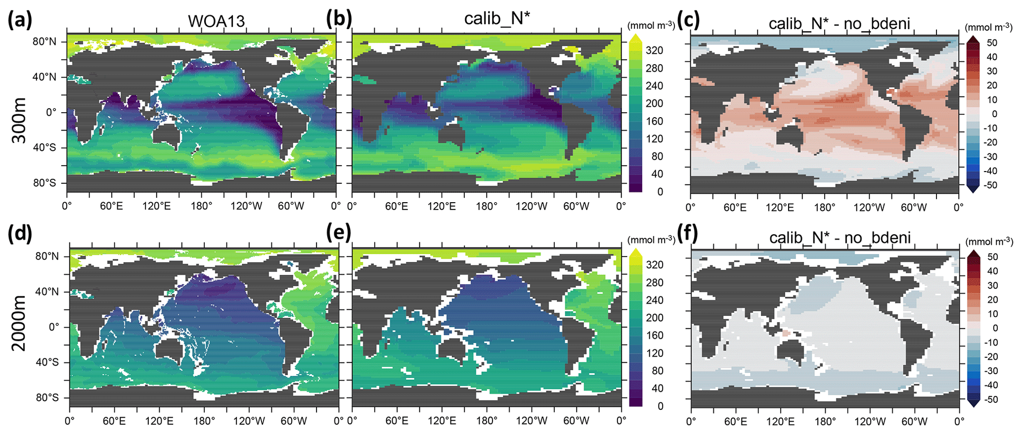
Figure 8 Spatial distribution of oxygen concentration at 300 and 2000 m for calib_N* and the changes in this new solution relative to no_bdeni.

The overestimation of O₂ in calib_N* compared to WOA13 at 2000 m occurs mainly in the Pacific Ocean, and the change relative to no_bdeni at this depth is spatially homogeneous. While our model solutions show consistent changes in O₂ concentration relative to no_bdeni that broadly point towards better agreement with observations at 300 m, changes are often in a direction diverging from observations at 2000 m (not shown). This finding is also reflected in the vertical profiles of globally averaged O₂ shown above (Fig. 6).

3.5 Global patterns of C fluxes

Our definition of global NPP includes the sum of phytoplankton NPP and diazotroph NPP. Export production (EP) is calculated as the product of the biomass of sinking particles and their sinking speed at 130 m depth. These sinking particles consist of detritus derived from phytoplankton, diazotrophs, and zooplankton. High production occurs in equatorial and subpolar regions (Fig. 9a and e), with the highest NPP found in the equatorial oceans. In contrast, EP in equatorial and subpolar oceans is comparable. The global distribution of export efficiency (EP$/$NPP, hereafter e-ratio) exhibits a negative relationship between NPP and the e-ratio. Low e-ratios (<0.2) occur in low latitudes, and high e-ratios (>0.2) occur in high latitudes, with a few exceptions in the Atlantic and Pacific subtropical gyres (Fig. 9i). Its general pattern is similar to the observational estimate of Dunne et al. (2005) and the model estimate of Henson et al. (2015). The low e-ratios of equatorial oceans result from elevated particle decomposition rates in high-temperature environments, owing to both increasing zooplankton respiration and detritus remineralization with temperature in our model.

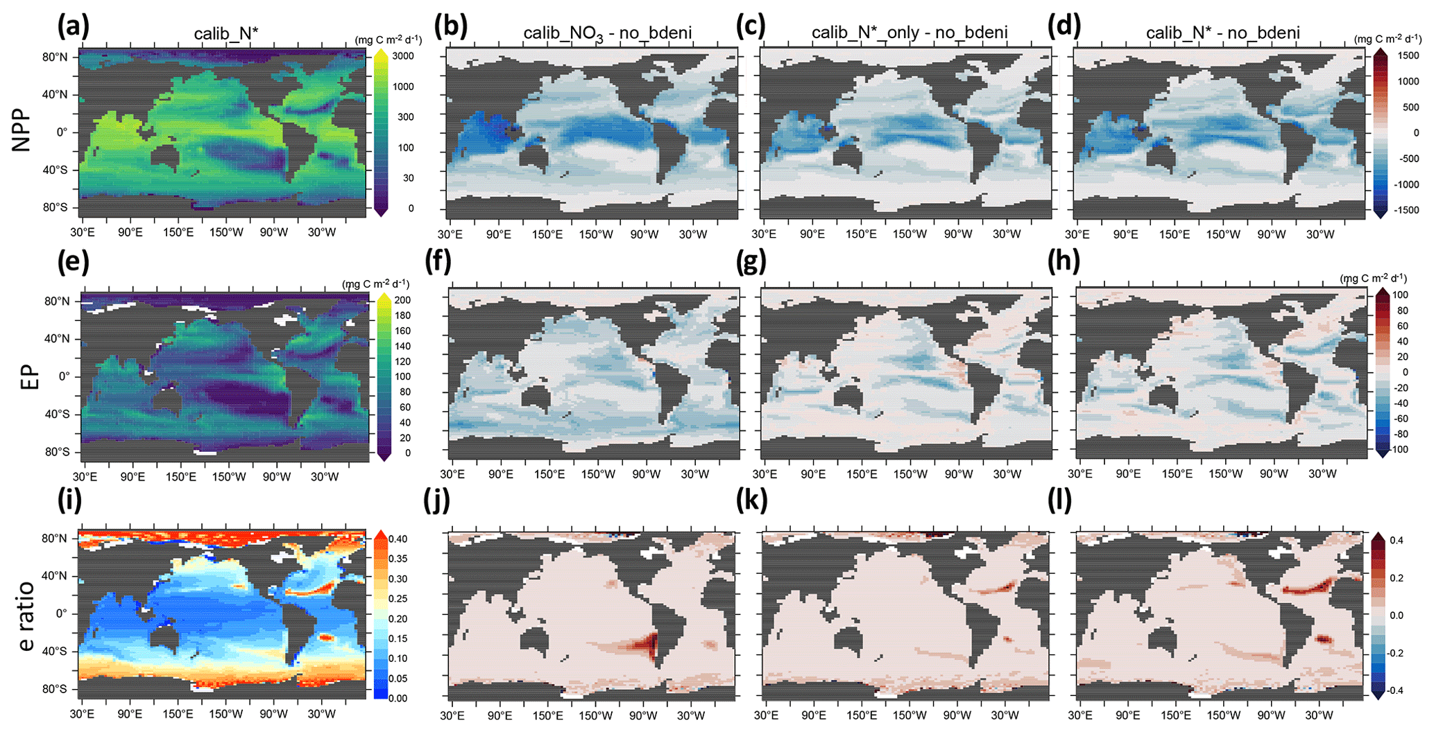
Figure 9 Vertically integrated net primary production (NPP), export production (EP) at 130 m, and e-ratio distributions for calib_N* and for the changes in three new solutions relative to no_bdeni.

Compared to no_bdeni, the new simulations exhibit notable decreases in NPP, mainly located in and adjacent to these high-production regions (Fig. 9b–d). While the primary pattern observed in the distribution of EP is a decline in most areas, there are some small areas that contain an increase (Fig. 9f–h). The decline in EP results in elevated concentrations of oxygen in the underlying subsurface ocean (Fig. 8c). Among the three solutions, calib_N* and calib_N*_only exhibit more similar patterns with each other than with calib_${\mathrm{NO}}_{\mathrm{3}}^{-}$.

4 Model and calibration limitations

In the northern Indian Ocean, our model shows an N* signal that is too low due to benthic denitrification at the Bay of Bengal, whereas the WOA13 data indicate an intense ODZ and a robust water-column denitrification in the Arabian Sea (Fig. 7d). This is likely due to underestimated coastal upwelling by the coarse model resolution in the Arabian Sea. An examination of CMIP5 models also reveals the presence of systematic deficiencies in the oceanic physics of these Earth system models (ESMs), resulting in an inaccurate representation of the east–west O₂ gradient in the northern Indian Ocean (Schmidt et al., 2021). The absence of a persistent ODZ in the Arabian Sea in our model is likely a reason why our global water-column denitrification and N₂ fixation rates are on the low end of observational estimates, between 131 and 253 Tg N yr⁻¹ (Großkopf et al., 2012; Luo et al., 2012; Landolfi et al., 2018; Shao et al., 2023).

The absence of an Arabian Sea ODZ may also be affected by the biome resolution of our calibration method, which has only one biome for the entire Indian Ocean, filtering out sub-basin variability. Sub-dividing the Indian Ocean biome might have the potential to improve the ability of the cost function to constrain O₂ and water-column denitrification. Future research building on high-resolution Earth system models may be amenable to choosing a spatially finer calibration in terms of 56 biogeochemical provinces (Longhurst, 2007). Concerning the unique characteristic of O₂ among tracers, an additional improvement would be to assume a normal distribution of O₂ concentration in the global ocean, which represents the data in WOA13 better than the log-normal distribution used here. However, since calib_N*_only chosen by cost_N* without calibrating against O₂ fails to reproduce the intense water-column denitrification in the northern Indian Ocean as well, further investigation is required.

The vertical distribution of N* shows that simulated N* tends to underestimate the observed N* at depth, particularly below 1000 m (Fig. 6c). There are some promising developments that could be implemented to improve the deep-ocean N* distribution. Our cost function metrics tend to focus on the upper ocean by including seasonal-scale variability only for the upper 550 m. This artificial emphasis on the upper ocean would be balanced by a refined volume-weighted cost function. In the current model configuration, the sinking velocity increases linearly with depth all the way to the ocean floor, which may lead to an overestimation of benthic denitrification in the deep ocean. A linear increase only up to 1000 m (Lam and Marchal, 2015) could give us a better representation of global carbon fluxes and corresponding benthic denitrification rates, which is the only plausible nitrogen loss flux that could occur below 1000 m (Fig. A1). Likewise, incorporating dissolved organic matter dynamics or preferential remineralization of phosphorus could assist in the reproduction of vertical gradients of N* (Somes and Oschlies, 2015). Improvements to the upper ocean may also have the potential to improve the deep-ocean performance, such as including the sinking speed of particles at the ocean surface (w_d0) in addition to its increase with depth (w_dd) in the calibrated parameters. By taking both w_d0 and w_dd into account for the calibration, the particle flux profile in our model could possibly be represented more accurately.

The influence of particle fluxes on N* via the effect on benthic denitrification leads to further discussion of the model uncertainties in the representation of benthic denitrification. A first uncertainty in the model estimate of benthic denitrification via the parameterization employed results from the uncertainties in the simulated bottom-water O₂ and ${{\mathrm{NO}}_{\mathrm{3}}}^{-}$ concentrations and the organic carbon rain rate. The accurate simulation of the rain rate is one of the most critical issues in ocean biogeochemistry and is associated with a high uncertainty (Clements et al., 2022; Kiko et al., 2017). A promising option could be to resolve the dependency of the remineralization rate on O₂, which could contribute to an accurate representation of the unique vertical profiles observed in ODZs (Pavia et al., 2019; Engel et al., 2022). Such efforts are necessary for a proper investigation of the relation between benthic denitrification and water-column denitrification. Moreover, the empirically derived parameterization of benthic denitrification itself is subject to a certain uncertainty, albeit to a lesser extent (Bohlen et al., 2012). Ocean physics introduces additional uncertainty. For example, the low physical resolution of the existing UVic model framework imposes relatively little computational demand, but the representation of N and C fluxes could benefit from a higher spatial resolution.

5 Conclusions

In order to explore the sensitivity to prior assumptions about which data are used for calibration, we applied our cost function to calibrate model solutions against three different combinations of observations. The best model solution calib_N* reaches the lowest cost function with the input of Chl, ${{\mathrm{PO}}_{\mathrm{4}}}^{\mathrm{3}-}$, O₂, and $\mathrm{N}\text{*}={{\mathrm{NO}}_{\mathrm{3}}}^{-}-\mathrm{16}{{\mathrm{PO}}_{\mathrm{4}}}^{\mathrm{3}-}+\mathrm{2.9}$. The model solution calib_N*_only shows significant parallels with calib_N* in various biogeochemical fluxes and tracers. Compared with the canonical cost function cost_${\mathrm{NO}}_{\mathrm{3}}^{-}$, which calibrates the model against Chl, ${{\mathrm{PO}}_{\mathrm{4}}}^{\mathrm{3}-}$, O₂, and ${{\mathrm{NO}}_{\mathrm{3}}}^{-}$, as was done previously (Pahlow et al., 2020; Chien et al., 2020), including N* provides better constraints on globally averaged N* and nitrate and also on globally integrated water-column denitrification and thus N₂ fixation. The greater constraining capacity of N* in comparison to considering nitrate and phosphate separately highlights the importance of accounting for correlations among variables within the cost function (Krishna et al., 2019) and demonstrates the power of diagnostic tracers such as N* for diagnostic studies of the ocean nitrogen cycle (DeVries et al., 2013; Eugster and Gruber, 2012; Deutsch et al., 2007).

UVic OPEM achieves a better representation of N₂ fixation and N* by incorporating benthic denitrification. Our model configurations demonstrate higher estimates of global N₂ fixation and an extension of N₂ fixation to higher latitudes in the Pacific, Atlantic, and Indian oceans compared to the simulation excluding benthic denitrification (no_bdeni). The calibrated model solutions calib_N* and calib_N*_only yield a global N₂ fixation of 137.7 and 136.1 Tg N yr⁻¹, respectively. The most apparent improvements in modeled N* distribution compared to WOA13 (Garcia et al., 2013a) are located in the surface layers of the North Pacific subpolar gyre, where consistently low N* signals result from the newly added benthic denitrification in the absence of local changes from other N fluxes and transfers. The improved representation of the global nitrogen cycle enables a more precise reproduction of net primary productivity. The estimated global integrated NPP, ranging from 52.8 to 63.0 Pg C yr⁻¹, is consistent with the estimates derived from satellite and Argo float observations (Silsbe et al., 2016; Johnson and Bif, 2021). The most significant decrease in NPP occurs in the tropical oceans, with a concomitant contraction of oxygen-deficient zones (ODZs). Benthic denitrification plays a globally important role shaping N₂ fixation and NPP throughout the global ocean and should be considered in marine biogeochemical models when trying to understand and predict changes in N₂ fixation and marine C fluxes.

Appendix A

Figure A1 Vertical profiles of the global averages of major N fluxes in the upper 1000 m.

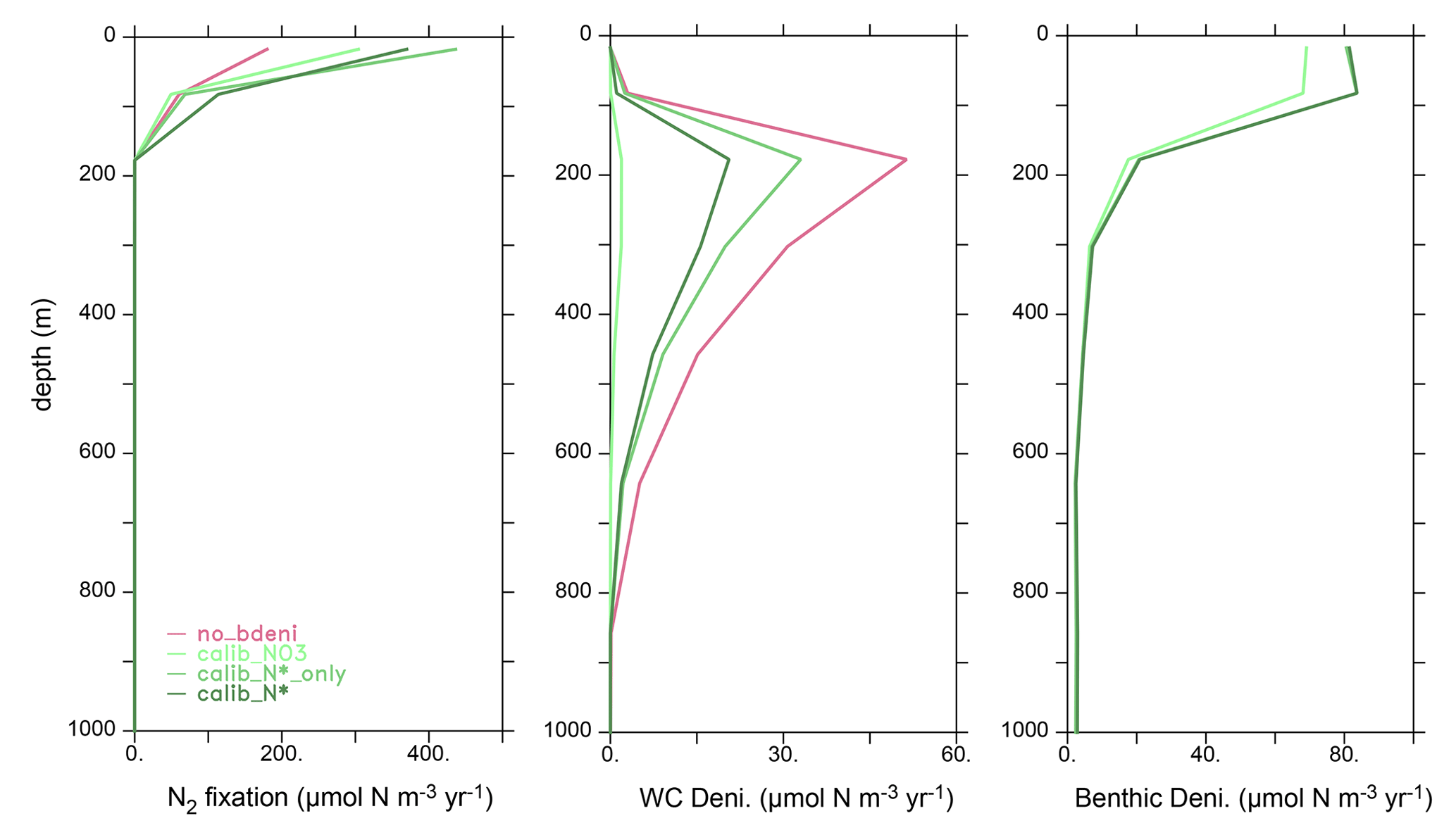
Table A1 Vertically integrated N fluxes; excess N relative to P in the organic matter (PON*); and average total excess N relative to P, including organic and inorganic forms ($\stackrel{\mathrm{‾}}{\text{TN*}}$) for ocean basins.

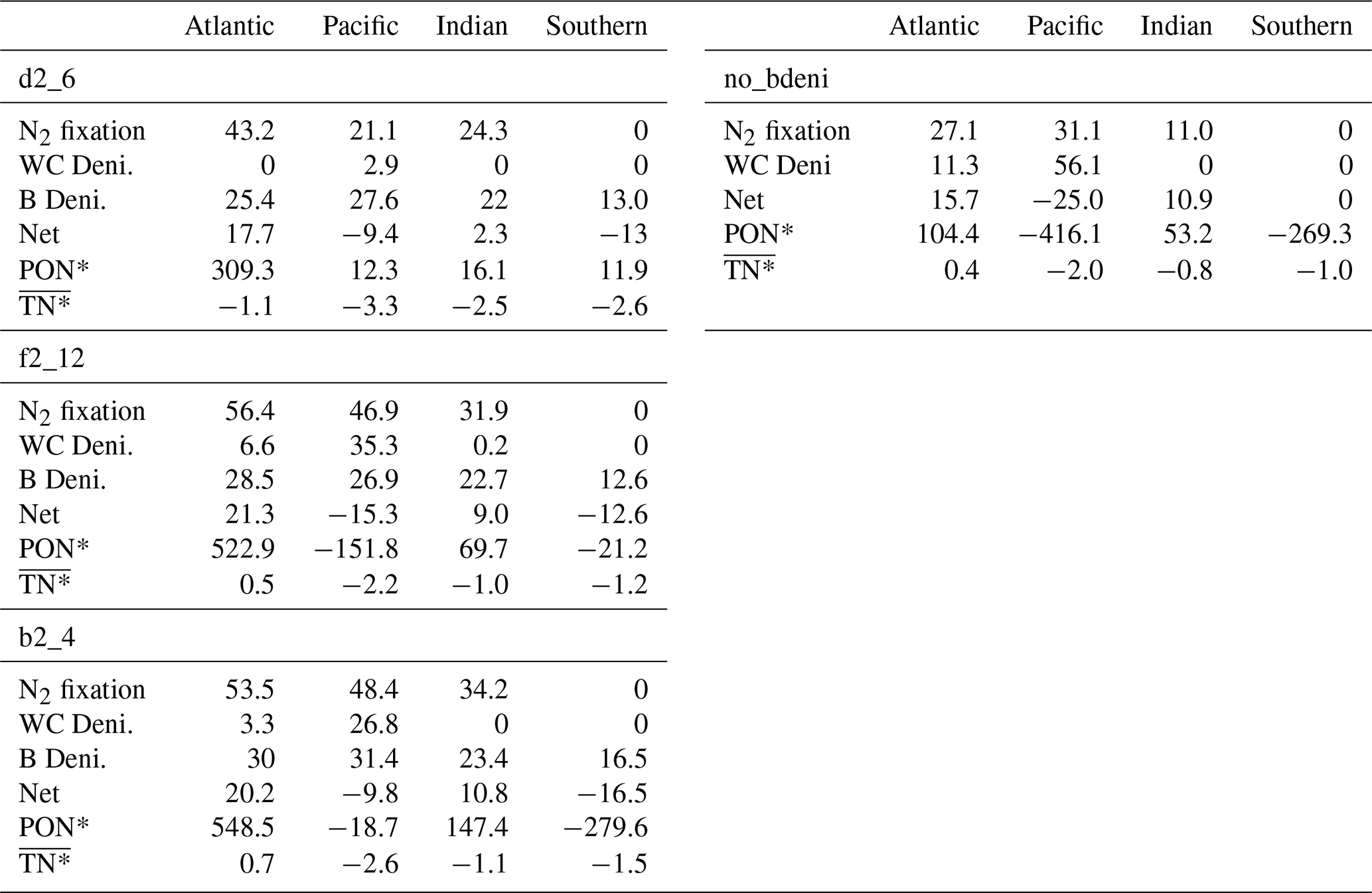
$\text{PON*}=\text{PON}-\mathrm{16}\times \text{POP}$, and $\text{TN*}=(\text{PON}+{{\mathrm{NO}}_{\mathrm{3}}}^{-})-\mathrm{16}\times (\text{POP}+{{\mathrm{PO}}_{\mathrm{4}}}^{\mathrm{3}-})+\mathrm{2.9}=\mathrm{N}\text{*}+\text{PON*}$. The unit for fluxes is Tg N yr⁻¹, and that of the vertically integrated PON* is 10¹² mmol m⁻³.