Dimethyl sulfide (DMS) climatologies, fluxes, and trends – Part 2: Sea–air fluxes

Dimethyl sulfide (DMS) contributes to cloud condensation nuclei (CCN) formation in the marine environment. DMS is ventilated from the ocean to the atmosphere, and, in most models, this flux is calculated using seawater DMS concentrations and a sea–air flux parameterization. Here, climatological seawater DMS concentrations from interpolation and parameterization techniques are passed through seven flux parameterizations to estimate the DMS flux. The seasonal means of calculated fluxes are compared to identify differences in absolute values and spatial distributions, which show large differences depending on the flux parameterization used. In situ flux observations were used to validate the estimated fluxes from all seven parameterizations. Even though we see a correlation between the estimated and observation values, all methods underestimate the fluxes in the higher range (>20 µmol m⁻² d⁻¹) and overestimate the fluxes in the lower range (<20 µmol m⁻² d⁻¹). The estimated uncertainty in DMS fluxes is driven by the uncertainty in seawater DMS concentrations in some regions but by the choice of flux parameterization in others. We show that the resultant flux is, hence, highly sensitive to both and suggest that there needs to be an improvement in the estimation methods of global seawater DMS concentration and sea–air fluxes for accurately modeling the effect of DMS on the atmosphere.

1 Introduction

Dimethyl sulfide (DMS) is a volatile organic compound obtained from its precursor, dimethylsulfoniopropionate (DMSP), through enzymatic cleavage (Andreae and Crutzen, 1997; Charlson et al., 1987; Simó, 2001; Yang et al., 2014; Abbatt et al., 2019; Galí and Simó, 2015). In seawater, DMS further undergoes biotic and abiotic processes. It is consumed by three major processes: (1) bacterial decomposition, (2) photolysis, and (3) ventilation to the atmosphere (Del Valle et al., 2009; Xu et al., 2019; Zhai et al., 2020). The last process is important as DMS in the atmosphere contributes to the formation of cloud condensation nuclei (CCN). Once DMS is released into the atmosphere from the sea surface, it is oxidized by hydroxyl radicals (OH), nitrate radical (NO₃), and halogen radicals (Br and Cl) to form sulfur dioxide (SO₂), methane sulfonic acid, and gas-phase sulfuric acid, which contribute to the formation of CCN (Andreae and Barnard, 1984; Woodhouse et al., 2010; Pazmiño et al., 2005). Hence, DMS is of importance in cloud formation and affects the climate due to its direct and indirect effect on radiative forcing (Yoch, 2002), although some uncertainties remain about its overall impacts and climate feedback (Quinn and Bates, 2011; Quinn et al., 2017).

Although the oceans are the major source of global DMS emissions, minor amounts of DMS have also been found to be emitted from vegetation on land (Vettikkat et al., 2020; Jardine et al., 2015; Yi et al., 2008). However, DMS emitted from the surface ocean is responsible for up to 70 % of the natural sulfur emissions into the global atmosphere (Andreae and Raemdonck, 1983; Carpenter et al., 2012; Hulswar et al., 2022). Considering this, it is important to develop a precise emission inventory for the assessment of climate impacts due to DMS emissions (Mahajan et al., 2015; Yang et al., 2015, 2017; Jin et al., 2018).

The emission of DMS occurs due to differences in the concentrations of DMS in the seawater and the atmosphere. The sea–air gas transfer is a complex process, with the wind having been proven to be one of the most influencing factors (Jahne et al., 1979; Frew et al., 2004; D'Asaro and McNeil, 2008; Blomquist et al., 2017). For example, DMS flux measurements have revealed a decrease in gas transfer at medium to high wind speeds (>10 m s⁻¹), attributed to wave–wind interactions and surfactant effects (Zavarsky et al., 2018), factors typically overlooked in traditional approaches (Bell et al., 2017). Hence, the sea–air gas transfer is parameterized as a function of wind speed. In an earlier comparison, Kettle and Andreae (2000) compared three parameterizations, viz. Liss and Merlivat (1986), Wanninkhof (1992), and Erickson (1993). They concluded that uncertainty in the flux parameterizations leads to uncertainties in estimating the global DMS flux. Furthermore, different datasets for wind speed, sea surface temperature (SST), and sea surface DMS concentration resulted in relatively small variations in these calculated fluxes (≤25 %) (Kettle and Andreae, 2000).

Here, we compare global sea–air DMS fluxes derived using seven different gas transfer velocity parameterizations using wind speed and SST. The comparison is conducted using different seawater DMS estimations to identify whether the uncertainty in the emissions is larger because of the uncertainty in seawater DMS concentrations or the flux parameterization. We use one interpolation-based seawater DMS concentration climatology (Hulswar et al., 2022, hereafter referred to as H22) and two parameterization-based seawater DMS climatologies (Galí et al., 2018, hereafter referred to as G18, and Wang et al., 2020, hereafter referred to as W20). A comparison between the three seawater DMS climatologies is presented in our companion paper (Joge et al., 2024). The comparison shows that there is a large difference between the interpolation- and proxy-based parameterization methods of estimating seawater DMS concentrations, with the interpolation-based method predicting higher values. Interestingly, both methods show an increase in DMS emissions over the last 2 decades. Here, we intercompared the DMS fluxes estimated using seven sea–air flux parameterizations and in situ DMS fluxes and identified the drivers of their uncertainties.

2 Data and methodology

For DMS flux calculation, seven parameterization schemes (LM86, Liss and Merlivat, 1986; E93, Erickson, 1993; N00a, N00b, Nightingale et al., 2000; Ho06, Ho et al., 2006; GM12, Goddijn-Murphy et al., 2012; W14, Wanninkhof, 2014) are used with the seawater DMS climatological data of H22, G18, and W20 (please check Joge et al., 2024). Each flux parameterization scheme uses wind speed, and some also use SST, to estimate the DMS sea–air flux. Wind speed and SST were obtained from the National Centers for Environmental Prediction (NCEP; https://psl.noaa.gov/data/gridded/index.html, last access: 9 January 2024) (Kalnay et al., 1996) and Centennial in situ Observation-Based Estimates (COBE; https://psl.noaa.gov/data/gridded/data.cobe.html, last access: 9 January 2024) (Ishii et al., 2005), respectively, for the years from 1948 to 2022, and then these were monthly averaged to calculate the fluxes. The in situ DMS flux observations measured by eddy covariance or gradient flux techniques were obtained from various studies carried out over the global oceans (Table S1 in the Supplement). The corresponding locations of flux observation data are shown in Fig. S5.

In general, all the parameterizations we compare in this study depend on wind speed (u) and the Schmidt number (Sc), which depends on temperature (T). The Schmidt number (Sc) is a dimensionless number defined as the ratio of kinematic viscosity (v) and molecular diffusivity (D), i.e., Sc $=v/D$ (Liss and Merlivat, 1986). The DMS sea–air flux is determined by using a bulk flux equation of F=k (C_w- C_a/H), where F is the calculated DMS flux; k is the gas transfer velocity; and C_w and C_a are the concentrations of the DMS in the seawater and the atmosphere adjacent to the seawater, respectively (Wanninkhof, 2014). H is Henry's law solubility for DMS in seawater, which varies with temperature, which is given as ln$H=-\mathrm{3547}/T+\mathrm{12.64}$ (Dacey and Wakeham, 1984). Here, C_a and C_w are measured in situ, while k depends on wind speed. C_w is several orders of magnitude higher than C_a; hence $C_{\mathrm{a}}/H$ is often ignored (Yan et al., 2023). It should be noted that previous studies have shown that C_a becomes important when the atmospheric boundary layer is shallow and the surface concentration is high (Steiner et al., 2006; Steiner and Denman, 2008). The flux parameterization methods give estimates of the k and Sc values, and we follow F=kC_w for DMS flux estimation with all seven flux parameterizations.

As wind is one of the most influential factors affecting gas transfer, most parameterizations have established different wind speed regimes for which different equations estimate the k values (Liss and Merlivat, 1986; Erickson, 1993). The gas transfer velocity k results from the waterside transfer velocity (k_w) and air-side transfer velocity (k_a). For the rarely soluble gas, air-side resistance is usually small and neglected, but DMS solubility increases with a decrease in temperature, and, hence, air resistance becomes important (Lana et al., 2011; Marandino et al., 2009; Omori et al., 2017). Most parameterizations agree that, at wind speeds less than 3.6 m s⁻¹, the surface is generally smooth with few waves, known as the “smooth-surface regime”. When the wind speed is above 3.6 m s⁻¹ but less than 13 m s⁻¹, it is known as the “rough-surface regime”, and more waves can be seen, enhancing the gas transfer. Above 13 m s⁻¹, this is known as the “breaking-wave regime”, where bubbles are formed along with the waves, dominantly increasing the flux, as evident from the Heidelberg circular-wind-tunnel experiments (Jähne et al., 1984; Jahne et al., 1979; Liss and Merlivat, 1986). The different flux parameterizations estimate the k value in those different wind regimes (u≤3.6: smooth-surface regime, $\mathrm{3.6}<u\le \mathrm{13}$: rough-surface regime, u>13: breaking-wave regime), and these wind regimes are also dependent on the Schmidt number (Sc) for each parameterization, where the Schmidt number depends on temperature (T).

2.1 Flux parameterization methods

2.1.1 LM86 flux parameterization

LM86 formulated the following equations for the three wind regimes, which are defined below following the results of the Heidelberg experiments (Jahne et al., 1979; Jähne et al., 1984).

$$\begin{array}{}\text{(1)}& {\displaystyle }{k}_{\mathrm{lm}\mathrm{86}}=\mathrm{0.17}\times \left(\mathrm{600}/S{c}_{\mathrm{lm}\mathrm{86}}\right)\mathrm{2}/\times u(u\le \mathrm{3.6})\text{(2)}& {\displaystyle }\begin{array}{rl}{k}_{\mathrm{lm}\mathrm{86}}& =\left(\mathrm{600}/S{c}_{\mathrm{lm}\mathrm{86}}\right)\mathrm{1}/\mathrm{3}\left(\mathrm{2.85}\times u-\mathrm{10.26}\right)+\mathrm{0.61}\\ & \times {\left(\mathrm{600}/S{c}_{\mathrm{lm}\mathrm{86}}\right)}^{\mathrm{2}/\mathrm{3}}(\mathrm{3.6}<u\le \mathrm{13})\end{array}\text{(3)}& {\displaystyle }\begin{array}{rl}{k}_{\mathrm{lm}\mathrm{86}}& ={\left(\mathrm{600}/S{c}_{\mathrm{lm}\mathrm{86}}\right)}^{\mathrm{1}/\mathrm{3}}\times (\mathrm{5.9}\times u-\mathrm{49.91})+\mathrm{0.61}\\ & \times {\left(\mathrm{600}/S{c}_{\mathrm{lm}\mathrm{86}}\right)}^{\mathrm{2}/\mathrm{3}}(u>\mathrm{13})\end{array}\end{array}$$

Here, u is the wind speed (in m s⁻¹) at 10 m above the sea surface. The Sc is based on the work carried out by Saltzman et al. (1993) and the references therein for the temperature range from 5 to 30 °C using

$$\begin{array}{}\text{(4)}& \begin{array}{rl}S{c}_{\mathrm{lm}\mathrm{86}}& =\mathrm{2674}-\left(\mathrm{147.12}\times \mathrm{SST}\right)+\left(\mathrm{3.726}\times {\mathrm{SST}}^{\mathrm{2}}\right)\\ & -(\mathrm{0.038}\times {\mathrm{SST}}^{\mathrm{3}}).\end{array}\end{array}$$

2.1.2 E93 flux parameterization

Erickson (1993) assumed that the sea surface is a mixture of a low-turbulence area (non-whitecap) and a high-turbulence area (whitecap). The gas transfer velocities are obtained from the radon outgassing data obtained during the expedition of Transient Tracers in the Ocean (TTO) and Geochemical Ocean Sections Study (GEOSECS) (Monahan and Spillane, 1984; Kettle and Andreae, 2000). The gas transfer velocities for other species are calculated using the following conversion formula based on wind speed ranges:

$$\begin{array}{}\text{(5)}& {\displaystyle }{k}_{e\mathrm{93}}=k_{R_n}\times {\left(S{c}_{e\mathrm{93}}/S{c}_{R_n}\right)}^{-\mathrm{2}/\mathrm{3}}(u<\mathrm{3.6}),\text{(6)}& {\displaystyle }{k}_{e\mathrm{93}}=k_{R_n}\times {\left(S{c}_{e\mathrm{93}}/S{c}_{R_n}\right)}^{-\mathrm{1}/\mathrm{3}}(u\ge \mathrm{3.6}).\end{array}$$

Here, $k_{R_n}$ (Monahan and Spillane, 1984) and Sc${}_{R_n}$ are the gas transfer velocity and Schmidt number for radon, respectively, which are given as follows:

$$\begin{array}{}\text{(7)}& {\displaystyle }{k}_{R_n}=\mathrm{2.3}+\mathrm{1.25}\times {\mathrm{10}}^{-\mathrm{3}}\times u^{\mathrm{3}}\left(u\text{in}{\mathrm{m}\mathrm{d}}^{-\mathrm{1}}\right),\text{(8)}& {\displaystyle }\begin{array}{rl}S{c}_{e\mathrm{93}}& =\mathrm{1911.3}-\mathrm{113.7}\times \mathrm{SST}+\mathrm{2.9}\times {\mathrm{SST}}^{\mathrm{2}}\\ & -\mathrm{0.029}\times {\mathrm{SST}}^{\mathrm{3}},\end{array}\text{(9)}& {\displaystyle }\begin{array}{rl}S{c}_{R_n}& =\mathrm{3147.3}-\mathrm{201.9}\times \mathrm{SST}+\mathrm{5.5}\times {\mathrm{SST}}^{\mathrm{2}}\\ & -\mathrm{0.055}\times {\mathrm{SST}}^{\mathrm{3}}.\end{array}\end{array}$$

2.1.3 N00a and N00b flux parameterization

Dual-tracer methods involving the measurements of sulfur hexafluoride SF₆ and 3-helium (³He) were also used to estimate k (Watson et al., 1991). Nightingale et al. (2000) describe the ideal dual-tracer combination as the one with one of the tracers being non-volatile, allowing dilution and dispersion corrections to be applied to the volatile tracer to minimize errors while estimating k. Due to the absence of such an ideal marine tracer, Nightingale et al. (2000) introduced a novel method of adding metabolically inactive bacterial spores of Bacillus globigii var. Niger as a conservative tracer to study the gas exchange in the North Sea (Watson et al., 1991; Nightingale et al., 2000), along with a SF₆ and ³He dual tracer for comparison. Combining data from other studies in George's Bank (Wanninkhof et al., 1993) and the West Florida shelf (Wanninkhof et al., 1997) with the North Sea data, the N00a parameterization coefficient was given as

$$\begin{array}{}\text{(10)}& k_{n\mathrm{00}a}=(\mathrm{0.222}\times u^{\mathrm{2}}+\mathrm{0.333}\times u)\times {\left(S{c}_{n\mathrm{00}a}/\mathrm{600}\right)}^{-\mathrm{0.5}}.\end{array}$$

However, this study exclusively had data from the northern Atlantic region. Coale et al. (1996) reported k values by using the dual tracer (SF₆/³He) in the equatorial Pacific Ocean, which was then used to upgrade the N00a parameterization to N00b; the upgraded parameterization is given as

$$\begin{array}{}\text{(11)}& \begin{array}{rl}{k}_{n\mathrm{00}b}& =(\mathrm{0.222}\times u^{\mathrm{2}}\times \text{shape\hspace{0.17em} parameter}+\mathrm{0.333}\times u)\\ & \times {\left(S{c}_{n\mathrm{00}b}/\mathrm{600}\right)}^{-\mathrm{0.5}}.\end{array}\end{array}$$

Here, the shape parameter is used to describe variations in wind speed using the Weibull distribution (Waewsak et al., 2011).

2.1.4 Ho06 flux parameterization

Ho et al. (2006) applied the dual-tracer technique to measure the gas transfer velocity with the wind speed ranging from 7 to 16 m s⁻¹. This was done during the Surface Ocean Lower Atmosphere Study (SOLAS) air–sea gas exchange (SAGE) campaign. The estimation of Ho06 was derived from the SAGE data, and the gas transfer coefficient is given as

$$\begin{array}{}\text{(12)}& k_{ho\mathrm{06}}=(\mathrm{0.266}\pm \mathrm{0.019})\times u^{\mathrm{2}}.\end{array}$$

2.1.5 GM12 flux parameterization

Goddijn-Murphy et al. (2012) argued that, since the wind does not directly affect the gas transfer, it is the turbulence caused as a result of wind that helps to form bubbles, which increases gas transfer. Hence, the sea surface roughness is a better parameter to quantify gas transfer. This study used satellite altimetry data to understand the sea surface roughness and measured the DMS gas transfer velocity using the eddy covariance flux determination from eight cruises. This resulted in the new GM12 parameterization, which gives the gas transfer velocity given as

$$\begin{array}{}\text{(13)}& k_{\mathrm{gm}\mathrm{12}}=\left(\mathrm{2.1}\times u-\mathrm{2.8}\right)\times {\left(S{c}_{\mathrm{gm}\mathrm{12}}/\mathrm{660}\right)}^{-\mathrm{0.5}}.\end{array}$$

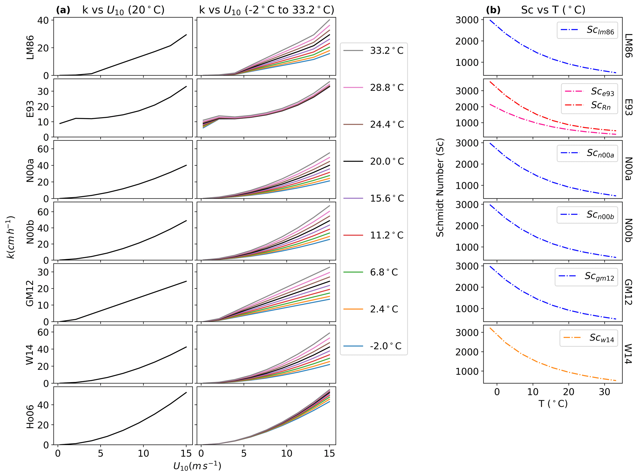
Figure 1 (a) Coefficient of gas transfer velocity (k) vs. wind speed at 10 m from sea surface (U₁₀) at constant temperature (20 °C) and at different temperature values (−2 to 33.2 °C). (b) Schmidt number (Sc) vs. temperature (T) for each flux parameterization method. Sc${}_{n{\mathrm{00}}_a}$, Sc_n00b, and Sc_gm12 have the same equation as Sc_lm86. Sc${}_{R_n}$ is the Schmidt number for radon used in the E93 parameterization. Schmidt number (Sc) decreases with an increase in temperature, and, hence, the gas transfer coefficient (k) increases.

2.1.6 W14 flux parameterization

Wanninkhof (1992) used the radiocarbon ¹⁴C data from the Red Sea (Cember, 1989) to understand the CO₂ gas exchange rates. Based on this, the parameterization was developed using the Sc number related to the work carried out by Saltzman et al. (1993), with the temperature range set between 18 to 25 °C. Further, with the help of better quantification of global wind fields and using data with a broader temperature range (−2 to 40 °C), the parameterization developed in 1992 is being upgraded using revised global ocean ¹⁴C inventories and an improved wind speed product (Wanninkhof, 2014). This new parameterization technique is known as W14, which gives a gas transfer velocity equation of

$$\begin{array}{}\text{(14)}& k_{w\mathrm{14}}=\mathrm{0.251}\times u^{\mathrm{2}}\times {\left(S{c}_{w\mathrm{14}}/\mathrm{660}\right)}^{-\mathrm{0.5}}.\end{array}$$

Here,

$$\begin{array}{}\text{(15)}& \begin{array}{rl}S{c}_{w\mathrm{14}}& =\mathrm{2855.7}-\mathrm{177.63}\times \mathrm{SST}+\mathrm{6.0438}\times {\mathrm{SST}}^{\mathrm{2}}\\ & -\mathrm{0.11645}\times {\mathrm{SST}}^{\mathrm{3}}+\mathrm{0.00094743}\times {\mathrm{SST}}^{\mathrm{4}}.\end{array}\end{array}$$

Sc_n00a, Sc_n00b, and Sc_gm12 have the same equation as Sc_lm86. LM86 shows three linear regions in the k vs. u plot, as defined by Eqs. (1)–(3). GM12 shows a linear dependency on the wind speed, while other equations show a nonlinear dependency (Fig. 1a). When temperature is changed from −2 to 33.2 °C, there is an increase and a spread between the k values. This is due to the temperature dependence of Sc, which nonlinearly decreases with temperature (Fig. 1b). Sc is the ratio of kinematic viscosity (v) and molecular diffusivity (D), i.e., Sc $=v/D$ (Liss and Merlivat, 1986). Thus, as Sc decreases with temperature, the molecular diffusion rate increases from higher concentrations (seawater) to lower concentrations (atmosphere), and, hence, the value of k increases with wind speed (Fig. 1). Note that, even though Ho06 is independent of Sc, there is a small spread in the values of k with temperature. This is due to the Ostwald solubility coefficient for DMS, defined according to McGillis et al. (2000), used in Ho06, and this coefficient depends on temperature.

Table 1 Area-weighted global mean flux standard deviation for each month and annually due to σ_DMS, σ_k, and σ_wind. Also, DMS_sulfur emissions for each month and annually from the areas with σ_DMS>σ_k and the area with σ_DMS<σ_k and the total emissions across the globe are computed using the N00b flux parameterization and the DMS climatology.

2.2 Estimation of uncertainties

The total uncertainty in DMS fluxes (σ_total) is calculated using the standard deviations in seawater DMS concentration (σ_DMS), the coefficient of parameterization (σ_k), and the wind speed (σ_wind):

$$\begin{array}{}\text{(16)}& {\mathit{\sigma }}_{\mathrm{total}}=\sqrt{{\mathit{\sigma }}_{\mathrm{DMS}}^{\mathrm{2}}+{\mathit{\sigma }}_k^{\mathrm{2}}+{\mathit{\sigma }}_{\mathrm{wind}}^{\mathrm{2}}}.\end{array}$$

Here, σ_DMS is calculated by calculating the standard deviation between H22, W20, and G18. This σ_DMS is used along with the N00b parameterization, wind speed, and SST data to estimate the standard deviation in the flux, which is shown in monthly and annual σ_DMS plots (Fig. S3). Next, σ_k is calculated by calculating the standard deviation between k from all seven flux parameterization equations, and this σ_k is further used, along with H22 seawater DMS climatology data, wind speed, and SST data, to get the standard deviation of the flux, which is shown in the monthly and annual σ_k plot (Fig. S4). Similarly, σ_wind is calculated by calculating the standard deviation between monthly global wind data from the different sources (NCEP Reanalysis 1, NCEP/DOE Reanalysis 2, ECMWF Reanalysis v5 (ERA5)), and it is used, along with the N00b parameterization, H22 seawater DMS climatology data, and SST, to calculate the standard deviation of the flux (plot is not shown; however, the area-weighted global mean is shown in Table 1). In this analysis, N00b is chosen as it has been used for previous DMS studies (Simó and Dachs, 2002; McNabb and Tortell, 2022; Zhang et al., 2021; Zhao et al., 2003, 2024; Lana et al., 2011; Hulswar et al., 2022) for the calculation of fluxes. Finally, σ_total is obtained using Eq. (16).

Figure 2 DMS fluxes estimated using the seven parameterizations for different seasons using the H22 climatology. The geographical pattern is similar in all the estimates, although the absolute values differ according to the parameterization chosen. In June–July–August (JJA), a maximum flux of 33.75 µmol m⁻² d⁻¹ is calculated in the Indian Ocean near Somalia with N00b. In December–January–February (DJF), a maximum flux of 45.82 µmol m⁻² d⁻¹ is calculated in the Weddell Sea region with E93.

3 Results

3.1 Salient features and seasonal variations

We estimated the seasonal DMS flux using seven different parameterizations and the global seawater DMS data of the H22 (Fig. 2), G18 (Fig. S1 in the Supplement), and W20 (Fig. S2) climatologies to study the geographical and seasonal variations and the differences between the parameterizations.

Overall, the fluxes estimated using all seven parameterizations follow the seawater DMS concentration distribution, with higher values in the Southern Hemisphere and the Northern Hemisphere in their respective summers (Fig. 2). Elevated levels are also seen in the Indian, Atlantic, and Pacific oceans in the extra-tropical regions, where elevated wind speed causes higher sea–air fluxes. While the geographical patterns are similar, there is a large difference in the absolute values among the different parameterizations. When using the G18 or W20 seawater DMS concentrations, the emissions show a similar difference among the different parameterizations, although the absolute values are lower (Figs. S1 and S2).

In December–January–February (DJF), E93 shows a maximum DMS flux of 45.82 µmol m⁻² d⁻¹ in the Weddell Sea region, where the maximum DMS concentration of 18.67 nM is also calculated in H22 (Joge et al., 2024). For E93, the flux is more uniformly distributed across the Southern Ocean as compared to the other parameterizations (Fig. 2). The other parameterizations also show elevated values in the Southern Ocean, although the range depends on the parameterization used. For example, the E93 parameterization results in the highest values, exceeding 20 µmol m⁻² d⁻¹ throughout the Southern Ocean, while the LM86 parameterization results in peak values of less than 10 µmol m⁻² d⁻¹. Further north, in other ocean basins such as the Indian Ocean, Ho06 and N00b predict relatively higher fluxes than E93.

During March–April–May (MAM), most parameterizations lead to elevated fluxes in the North Atlantic Ocean, Caribbean Sea, Baltic Sea, and North Sea, with the DMS flux ranging from 8.71 to 18.73 µmol m⁻² d⁻¹ using the H22 seawater DMS concentrations. Higher fluxes are also calculated on the western coast of the American continent and in the coastal regions of Africa. The gyres in the equatorial Pacific and Indian oceans also show higher fluxes, although the North Atlantic Ocean has higher fluxes than the other ocean basins. Although all the parameterizations show higher values in the Northern Hemisphere, E93 shows the highest fluxes, and the LM86 parameterization shows the lowest fluxes. In a similar manner, N00b shows high flux values (13.8 µmol m⁻² d⁻¹) compared to N00a (11.33 µmol m⁻² d⁻¹) in the Caribbean Sea, probably due to the wind correction factor in the N00b parameterization.

The June–July–August (JJA) period shows high values in the upwelling regions off the continental coasts and in the equatorial Indian Ocean and the Pacific Ocean. During this period, the geographical variation strongly depends on the parameterization chosen. For example, the E93 parameterization mainly shows peaks in the Arctic Ocean and the northern boundaries of the other ocean basins. However, other parameterizations show peaks in the equatorial oceans in addition to at the northern latitudes. This difference in variation is driven by the different responses of the parameterizations to winds.

Flux values start increasing in the Southern Ocean during September–October–November (SON). The flux value estimated by Ho06 was the highest during this period (18.40 µmol m⁻² d⁻¹) in the South Atlantic Ocean along coastal areas of South Africa, although the other parameterizations also show an increase in the Southern Ocean, except for LM86. A distinct hotspot is also seen in the Indian Ocean region in all estimations, specifically in Ho06, followed by N00a (13.77 µmol m⁻² d⁻¹), N00b (16.75 µmol m⁻² d⁻¹), GM12 (11.97 µmol m⁻² d⁻¹), and W14 (13.84 µmol m⁻² d⁻¹), while LM86 estimated the lowest flux value (10.66 µmol m⁻² d⁻¹) in the Indian Ocean region.

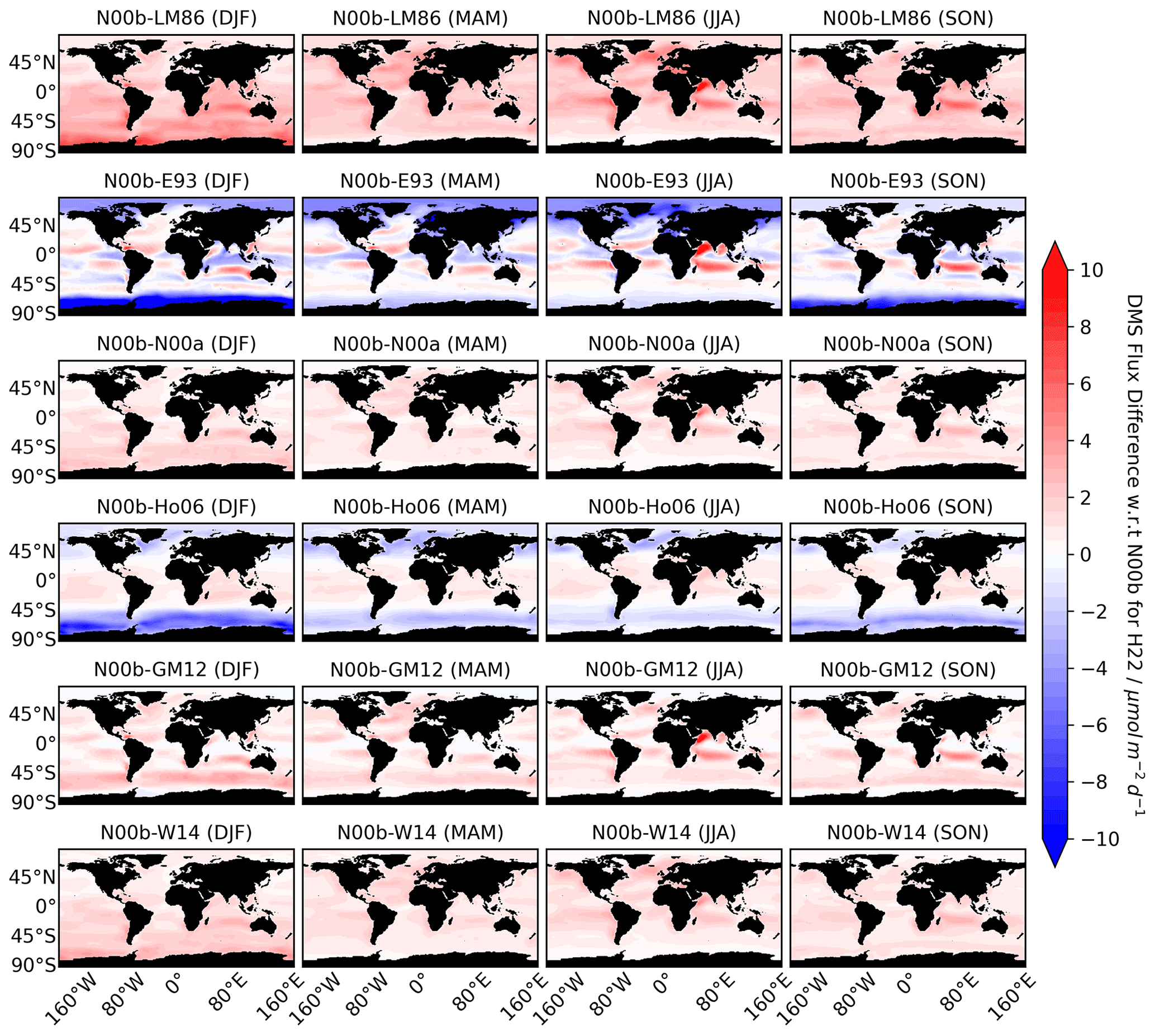
Figure 3 Differences between the DMS fluxes estimated using N00b parameterization and the remaining six parameterizations. For all the seasons (December–January–February (DJF), March–April–May (MAM), June–July–August (JJA), September–October–November (SON)), N00b–LM86 shows a positive difference, while the other parameterizations (E93, Ho06) show negative differences in the Southern Ocean and the Arctic region, although some positive differences are also present in E93 and Ho06 in mid-latitude regions. GM12, W14, and N00a show small positive differences when subtracted from N00b, while N00b–LM86 shows a notable large positive difference. The summary of the differences in different oceanic regions is listed in Table S2.

3.2 Differences

We calculated the seasonal differences between all the flux parameterizations with respect to the N00b (Fig. 3); however, the DMS–CO₂ flux usually uses the W14 flux parameterization, but we choose N00b as it is used in the recent DMS climatology papers (Zhao et al., 2024; Wang et al., 2020; Hulswar et al., 2022; Lana et al., 2011). Annually, the largest positive difference is seen in the LM86 parameterization, which consistently displays lower values than the N00b parameterization due to the linear dependence of wind speed in LM86 and the quadratic wind speed in N00b (Eqs. 1–3 and 11). The largest negative differences in the polar regions are present in the E93 parameterization, which shows that higher values are calculated for those regions than in the N00b parameterization. Although Ho06 also shows large negative differences in the polar regions, large positive differences are present in the mid-latitude and coastal regions. These differences can be as much as 100 % in certain regions, showing that the choice of parameterization plays a crucial role in the DMS flux estimates. The largest positive differences are present in N00b–LM86 in all the seasons, while the largest negative differences can be seen with N00b–E93 (Fig. 2). This large negative difference is driven by the differences in the high-latitude regions where N00b does not show peaks, for example, in the Southern Ocean (Fig. 2). In the mid-latitude and the equatorial regions, peaks are present in N00b estimations, and, hence, N00b–E93 shows the largest positive differences, as listed in Table S2. Although N00b is upgraded from the N00a parameterization, there is no negative difference between the two parameterizations (Fig. 3), which indicates that N00b estimates higher flux values than N00a (Fig .2). The maximum positive differences between the two are listed in Table S2 for all seasons. The differences between N00b and Ho06 are primarily negative (Table S2), but the positive differences are also present in the range from 1.5 to 2.37 µmol m⁻² d⁻¹ but are lower than for N00b–N00a. The difference between N00b and GM12 is positive. Similarly, in the case of N00b–W14, positive differences are present, which can be clearly seen from Fig. 3. The summary of the maximum positive and negative values of differences in different oceanic regions is given in Table S2.

3.3 Drivers in flux uncertainties

As explained in the “Data and methodology” section, the total uncertainty in DMS fluxes is derived from the uncertainty in the seawater DMS concentrations, parameterization, and wind speed.

Figure S3 shows the standard deviation in the DMS flux calculated using the standard deviation between climatological seawater DMS concentrations (σ_DMS) of G18, W20, and H22. Here, the sea–air parameterization is kept constant to isolate the effect of the change due to seawater DMS concentrations. The monthly climatological wind speed data (NCEP Reanalysis 1) are used for the flux estimation. From Table S3, the maximum σ_DMS can be seen in December, January, and February in the South Atlantic Ocean compared to being seen in the June, July, and August months in the North Atlantic Ocean and the Arabian Sea. Overall, the largest standard deviation in σ_DMS can be seen in the Southern Ocean (Fig. S3), where the DMS concentrations are the largest. Figure S4 shows the standard deviation in the DMS flux due to the standard deviation among seven gas transfer velocity coefficients (σ_k). Here, we keep the seawater DMS concentrations constant (H22), and the monthly climatological wind speed data of the NCEP Reanalysis 1 are used. The maximum σ_k can be seen in December, January, and February in the Weddell Sea region compared to being seen in the June, July, and August months in the Indian Ocean region (Table S3). From Figs. S3 and S4, it can be seen from comparison that σ_k is dominant over σ_DMS in the Weddell Sea region, as well as across the coast of the Antarctic region. Apart from this coastal region in Antarctica, other coastal regions are dominated by σ_DMS.

Figure 4 An estimate of the total variation (σ_total) in the flux emission, which is shown as a background map and is obtained from the standard deviations in the seawater DMS concentrations (σ_DMS), the standard deviations in the coefficients of parameterizations (σ_k), and the variation due to wind speed (σ_wind). σ_wind has a small contribution compared to σ_DMS and σ_k (Table 1). The regions where seawater DMS concentrations drive the uncertainty are indicated by red dots (σ_DMS>σ_k), while, in the other areas (no red dots), it is driven by the variation due to the choice of the flux parameterization (σ_DMS<σ_k). The maximum values of σ_total are listed in Table S3.

Further, the standard deviation in the DMS flux is estimated by calculating the standard deviation of the wind speed (σ_wind) obtained from different sources. The area-weighted global mean flux standard deviation due to σ_wind is much lower than the area-weighted global mean flux standard deviation due to σ_DMS and σ_k on monthly and annual scales (Table 1). Also, from Table S3, it can be seen that the maximum σ_wind is less in all the months and on the annual scale compared to σ_DMS and σ_k even though these values are from different oceanic regions. This shows that the total standard deviation of the sea–air DMS flux (σ_total) is dominated by σ_DMS and σ_k, with σ_wind playing a minor role in the total flux uncertainty (Tables S3 and 1).

The climatological monthly and annual σ_total values are shown in Fig. 4. The maximum σ_total values in different oceanic regions are shown in Table S3. In most of the months, it can be seen that, for the oceanic regions where σ_total is at maximum, σ_DMS is also at maximum, while, for some of the months, σ_k is at maximum. Thus, there is a big contribution to σ_total by both σ_DMS and σ_k, but, for most of the regions, σ_DMS shows the primary contribution, while σ_wind makes a minor contribution. In Fig. 4, the regions where the σ_total is dominated by the variation in seawater DMS concentrations, i.e., σ_DMS>σ_k, are indicated by red dots. The regions where the red dots are absent are the ones where the dominant contribution to σ_total is due to σ_k. Also, σ_total values in oligotrophic oceans and most of the coastal areas are dominated by σ_DMS. Annually, the σ_total in the Southern Ocean is dominated by σ_DMS, but that in the coastal area of Antarctica is dominated by σ_k. Table 1 also shows the total DMS_sulfur flux to the atmosphere according to each month and annually averaged. For most of the year, the total flux from regions where σ_DMS is greater than σ_k is larger. Indeed, the total annual flux of DMS_sulfur to the atmosphere is estimated to be 22.08 Tg, of which 17.16 Tg is contributed by areas where σ_k<σ_DMS. This indicates that, on an annual scale, the uncertainty in DMS_sulfur emissions is dominated by seawater DMS concentration. However, from Fig. 4, the choice of the flux parameterization also contributes a considerable amount of uncertainty in the coastal areas of Antarctica, which can be seen in November, December, January, and February. Overall, the choice of the seawater DMS estimation method has a larger influence on sea–air DMS flux than the choice of flux parameterization, which is also corroborated by analyses presented by Bhatti et al. (2023) and Tesdal et al. (2016).

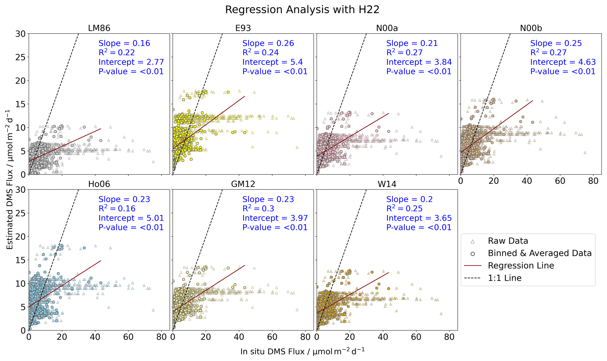
Figure 5 Comparison of in situ and estimated DMS fluxes (using H22) with the different parameterizations. Here, the regression analysis is done with binned and averaged in situ data at 1°×1° resolution as the flux climatologies are also at the same resolution. The analysis shows that flux calculations result in higher fluxes than observations at low levels (<20 µmol m⁻²,d⁻¹) and lower fluxes than observations at higher levels (>20 µmol m⁻² d⁻¹), which indicates that flux parameterization methods fail to represent the range accurately. The dashed black line is the 1:1 representation between the in situ and the estimated DMS flux points, and the dark-red line is the regression line. A list of the in situ observations used for the comparison is given in Table S1.

3.4 Comparison with in situ observations

In situ DMS flux data were compared with the co-located DMS flux data estimated from different parameterizations using the H22 (Fig. 5), G18 (Fig. S6), and W20 (Fig. S7). The raw in situ data points are localized and inconsistent in terms of temporal and spatial resolution, while models provide the average. Thus, raw in situ flux data points are not comparable with the model flux values calculated with parameterizations. Hence, for the analysis, raw in situ DMS flux data are binned to a 1°×1° resolution grid box for each month, and then, flux data points within that box are averaged. Due to binning and averaging, localized in situ information may be lost, but for the comparison with DMS flux calculated with parameterization models, this is the nearest traditional method. After this, ordinary least-square regression is applied. For reference, raw in situ DMS flux points are shown in the background (Figs. 5, S6, and S7). All flux estimates using either of the DMS seawater climatologies, with any of the flux parameterizations, struggle to match the observations.

In most cases, the flux estimations in the lower range (<20 µmol m⁻² d⁻¹) are overestimated, while the values are underestimated in the higher range (>20 µmol m⁻² d⁻¹). Indeed, in all the cases, a positive intercept in the linear regressions shows that the emissions are overestimated at lower flux values. This would indicate a constant background flux in the estimated emissions, which would overestimate the total DMS_sulfur flux to the atmosphere. In contrast, the fact that the flux estimates do not reproduce the higher DMS fluxes indicates that high-emission scenarios, which would contribute strongly to new particle formation and growth, are underestimated by the emission estimations. It should be noted that we use monthly seawater DMS concentration fields as input. Hence, a difference between the observations and estimations is expected, but there is consistent overestimation of model flux for the lower-range (0.1 to <20 µmol m⁻² d⁻¹) in situ flux points and underestimation for the higher-range (>20 to 43.4 µmol m⁻² d⁻¹) in situ flux points. The best match in the lower range is found when using the W20 seawater DMS estimations (Fig. S7), although the slope is consistently lower than 0.33, and the intercept is higher than 2.17 µmol m⁻² d⁻¹ for all the flux parameterizations (R²<0.32 for all the parameterizations). Both H22 and W20 perform better than G18, but none of the correlation coefficients are found to be important, and all the flux parameterization methods fail to reproduce the in situ DMS flux values, particularly the high values of fluxes (Figs. 5, S6, and S7).

4 Discussion

This study has been conducted to quantify the factors that contribute to the total uncertainty in DMS fluxes to the atmosphere. From our analysis, it was found that the total uncertainty in the DMS fluxes is dominated by the uncertainty in the seawater DMS concentrations, followed by the coefficient of the gas transfer velocity used in flux parameterization equations. The uncertainty due to wind speed is negligible in comparison.

The seawater DMS concentrations estimated by G18, W20, and H22 have large differences between themselves (please check Joge et al., 2024). This is a major source of uncertainty and shows the need for more detailed long-term observations across different ocean basins. The present available observations are not consistent in terms of temporal and spatial resolution, and some regions like the Southern Ocean are highly under-sampled but very important due to high DMS emissions. Hence, models do not fully capture the seawater DMS variations, which translate into uncertainty in the emissions.

In addition to seawater DMS observations, which we hope will be undertaken in the future, there are some regions where uncertainty in the total DMS flux is mostly due to the k values. From k vs. u plots (Fig. 1a) of the seven flux parameterization methods, it is seen that there are large differences among these seven methods. In LM86, N00a, N00b, GM12, and W14, there is a spread in the values of k due to the Schmidt number (Sc). This spread arises from the SST. Even though E93 uses this Sc number, the spread is smaller compared to other parameterizations, while there is negligible spread in Ho06. To calculate the DMS flux, at present, we do not use the C_a values as we assume that DMS is supersaturated in seawater. However, past studies have shown that, in some special cases, such as when the atmospheric boundary layer is shallow on cold nights or in winter, it is important to consider the air-side DMS concentration. In one of the model studies, it was found that the difference in the emissions in considering C_a can be as high as 50 % (Steiner and Denman, 2008; Steiner et al., 2006), which adds to the uncertainty. The k vs. u plots (Fig. 1a) are comparable between the seven parameterizations, and the total uncertainty due to wind speed from different sources is negligible. Like in situ DMS observations, in situ flux observations are important in order to develop more accurate flux parameterizations. Observations collected from the different flux techniques, such as eddy covariance and gradient flux, can add to the uncertainty in flux observation data, and cross-comparison between the methods across a range of fluxes needs to be undertaken.

The gas transfer velocity equation of W14 uses the square of the average neutral-stability winds at 10 m height or the second moment, i.e., average of the quadratic wind speed. In this study, we used monthly average wind speed, i.e., quadratic of the average wind speed for W14. The first method of calculation will estimate higher k values than the second one due to the averaging of the winds. We checked the differences between the two and found that the maximum difference is not more than 4.3 cm h⁻¹ for the June, July, and August months, and it is less than 2 cm h⁻¹ for the rest of the year, which does not contribute pointedly to the large uncertainty.

From 1998 to 2010, both G18 and W20 show an increasing trend in seawater DMS (Joge et al., 2024). Using the calculated seawater DMS concentrations, G18 and W20 DMS flux trends are also calculated for each parameterization method using the bootstrap resampling method (explained in Joge et al., 2024). The DMS flux trend also shows an increase for all the parameterizations (Figs. S8 and S9). DMS flux values are between 3 and 6 µmol m⁻² d⁻¹ for E93 and Ho06, but they are lower in LM86. GM12 and W14 show a similar range, while N00b shows a larger range compared to N00a.

The DMS flux derived from both empirical and prognostic models shows the poor agreement with fluxes from the point observations (Tesdal et al., 2016), which can also be seen with the flux parameterization methods used in this study when compared with the in situ DMS flux observations (Fig. 5). Tesdal et al. (2016) also concluded that there is large uncertainty in the temporal and spatial distribution of DMS concentrations and fluxes. The total sea–air DMS flux depends primarily on the global mean surface ocean DMS concentrations, and the spatial distribution of the DMS concentration and the magnitude of the gas exchange coefficient are of secondary importance. In our study, it is primarily seawater DMS concentrations that need to be estimated accurately as σ_DMS dominates over σ_k in most of the regions of global ocean, but, for some regions, it is important to consider σ_k over σ_DMS, which agrees with the study of Tesdal et al. (2016).

5 Conclusions

The sea–air DMS flux was estimated using different seawater DMS climatologies (see Joge et al., 2024), wind, and SST values as inputs into seven different flux parameterizations. All the flux estimations show a similar seasonal variation, with peaks in the summers of each hemisphere. However, there were large geographical and absolute flux differences among the different estimations, showing that the DMS_sulfur flux to the atmosphere is sensitive to the chosen seawater DMS fields and the chosen flux parameterization. The total uncertainty in flux estimation is dominated by the uncertainty in seawater DMS concentrations and the choice of flux parameterization, while the effect on the total uncertainty due to the different sources of wind speed is less important; however, this might not be true when comparing to in situ fluxes as the gustiness of wind might play an important role. In certain parts of the globe, such as the Peru upwelling region, the South Pacific Ocean, the Indian Ocean, the Arabian Sea, the Bay of Bengal, continental coastal regions, the North Atlantic Ocean, the Gulf of Alaska, and the Southern Ocean, the differences between the climatological estimated seawater DMS of G18, W20, and H22 can be seen in the figures (Joge et al., 2024). Hence, the uncertainty in the total flux emission is dominated by the uncertainty due to the seawater DMS concentration in these areas, where the differences are important (Fig. 4). In other regions, uncertainty is dominated by the choice of the coefficient of the flux parameterization, such as in the coastal area of Antarctica and the Arctic Ocean. A comparison of in situ and co-located estimated fluxes showed that all the parameterizations overestimate the DMS flux below 20 µmol m⁻² d⁻¹ but underestimate fluxes larger than 20 µmol m⁻² d⁻¹. This suggests that emissions in current models overestimate the total sea–air DMS flux but underestimate that in the higher range (>20 to 43.4 µmol m⁻² d⁻¹) when this can impact new particle formation and growth.