Seasonal dynamics and regional distribution patterns of CO₂ and CH₄ in the north-eastern Baltic Sea

Significant research has been carried out in the last decade to describe the CO₂ system dynamics in the Baltic Sea. However, there is a lack of knowledge in this field in the NE Baltic Sea, which is the main focus of the present study. We analysed the physical forcing and hydrographic background in the study year (2018) and tried to elucidate the observed patterns of surface water CO₂ partial pressure (pCO₂) and methane concentrations (cCH₄). Surface water pCO₂ and cCH₄ were continuously measured during six monitoring cruises onboard R/V Salme, covering the Northern Baltic Proper (NBP), the Gulf of Finland (GoF), and the Gulf of Riga (GoR) and all seasons in 2018. The general seasonal pCO₂ pattern showed oversaturation in autumn–winter (average relative CO₂ saturation 1.2) and undersaturation in spring–summer (average relative CO₂ saturation 0.5), but it locally reached the saturation level during the cruises in April, May, and August in the GoR and in August in the GoF. The cCH₄ was oversaturated during the entire study period, and the seasonal course was not well exposed on the background of high variability. Surface water pCO₂ and cCH₄ distributions showed larger spatial variability in the GoR and GoF than in the NBP for all six cruises. We linked the observed local maxima to river bulges, coastal upwelling events, fronts, and occasions when vertical mixing reached the seabed in shallow areas. Seasonal averaging over the CO₂ flux suggests a weak sink for atmospheric CO₂ for all basins, but high variability and the long periods between cruises (temporal gaps in observation) preclude a clear statement.

1 Introduction

Carbon dioxide (CO₂) and methane (CH₄) are important atmospheric greenhouse gases influencing the global climate. Changes in the levels of these trace gases are monitored in comparison with the pre-industrial era; however, precise and systematic atmospheric CO₂ and CH₄ measurements were not started before the late 1950s and early 1980s, respectively (Keeling et al., 2009; Dlugokencky et al., 1994). In the recent decade (2012–2021), the atmospheric CO₂ growth rate was 5.2 ± 0.02 GtC yr⁻¹ (Friedlingstein et al., 2022). Atmospheric concentration of CH₄ remained nearly constant from the late 1990s through 2006 but resumed increasing since then at an average rate of 7.6 ± 2.7 ppb yr⁻¹ estimated for 2010–2019 (Canadell et al., 2023). Methane has large emissions from both natural (e.g. wetlands) and anthropogenic (e.g. enteric fermentation, manure treatment, fossil fuel exploitation) sources, but a clear demarcation of their nature is difficult (Canadell et al., 2023).

The global ocean is estimated to be a net sink of CO₂ (26 % of total CO₂ emissions during the decade 2012–2021; Friedlingstein et al., 2022). However, these global estimates are only beginning to resolve the net CO₂ source–sink characteristics of the coastal ocean. The complexity of processes in the coastal ocean and the limited data availability make it difficult to quantify regional carbon budgets and the coastal ocean's role in the global carbon budget. Although oceanic methane emissions play a modest role in the global methane budget (Reeburgh, 2007), estuaries and other coastal areas contribute up to 75 % of all oceanic CH₄ emissions (Bange et al., 1994), with an important but not well-quantified contribution of very shallow waters (Borges et al., 2016).

The exchange at the air–sea interface is controlled by the air–sea difference in gas concentrations (CO₂ or CH₄) and by the efficiency of the transfer processes. In the Baltic Proper, the seasonal cycle of CO₂ is characterized by changing saturation levels between different seasons: oversaturation during autumn and winter and considerable undersaturation during spring and summer (Thomas and Schneider, 1999). Spring and summer periods are characterized by two distinct minima attributed to the spring phytoplankton bloom and the cyanobacteria bloom in midsummer, respectively (Schneider et al., 2014; Schneider and Müller, 2018). Understanding the surface water CO₂ dynamics in the Baltic Sea is becoming increasingly important since it is tightly linked to the biogeochemical processes, including primary production and nutrient (nitrogen and phosphorus) dynamics. In addition to the exchange at the air–sea interface and biological processes, the CO₂ system of surface waters in the Baltic Sea is influenced by the changes in hydrological and hydrographic conditions, e.g. river discharges, waves, currents, salinity and temperature, vertical stratification and mixing, upwelling and downwelling, and fronts (e.g. Müller et al., 2016; Jacobs et al., 2021).

Methane is formed by microbial methanogenesis during the decomposition of organic material. CH₄ generated in the sediments that is not consumed at the sediment–water interface can diffuse into the water column and be transported over large areas of the Baltic Sea (e.g. Gülzow et al., 2014). CH₄ is consumed while approaching the surface water due to methane oxidation at the redoxcline and in the oxygenated water column above (Schmale et al., 2010; Jakobs et al., 2013, 2014). This leads to strong vertical stratification with elevated concentrations in the sub-redoxcline layer and concentrations near atmospheric equilibrium at the sea surface (e.g. Schmale et al., 2010). Methanogenesis is generally more prevalent in shallower coastal regions due to the higher organic matter content (Valentine, 2002). In coastal areas, the dominant controlling factors for the seasonal variations in methane emission are the sediment organic matter content (Heyer and Berger, 2000), which might be modulated by seasonal deposition of fresh organic material from primary production, and temperature (Borges et al., 2018). In areas where the water column is relatively shallow and constantly mixed, CH₄ may escape into the atmosphere more readily. In general, the Baltic Sea is a source of atmospheric CH₄ (Bange et al., 1994; Gülzow et al., 2013), with the majority of methane emissions coming from shallow coastal areas (e.g. Roth et al., 2022). Outgassing can be intensified as a consequence of high water temperatures (Humborg et al., 2019) and processes driving vertical transport and mixing, e.g. upwelling events (Jacobs et al., 2021). Production in the upper, oxygenated water column might also contribute to or even govern methane sea–air fluxes (Schmale et al., 2018; Stawiarski et al., 2019), but it is of minor importance in the coastal ocean (Weber et al., 2019) and negligible in shallow coastal areas of high methane concentrations and emissions.

This work is the first extensive trace gas (CH₄ and CO₂) study in the north-eastern Baltic Sea area, with the main focus being on the southern Gulf of Finland (GoF) and the Gulf of Riga (GoR), allowing the assessment of surface layer trace gas and carbon system dynamics in the region. The main aim of our work is to describe the spatial variability and seasonal dynamics of CO₂ and CH₄ and compare these patterns with the better-studied Northern Baltic Proper (NBP) (Schneider et al., 2014; Schneider and Müller, 2018; Jakobs et al., 2014; Gülzow et al., 2013). We analysed the physical forcing and hydrographic and biological background in the study year (2018) and made an effort to link the observed patterns of CO₂ and CH₄ to these drivers.

The questions we try to answer are as follows. Is the seasonal cycle of CO₂ and CH₄ in the southern GoF and GoR similar to that in the NBP? Can we elucidate regional differences in CO₂ and CH₄ dynamics due to river discharges, water depth and mixing, fronts and upwelling events, or other hydrographic features? Do the regional variations in CO₂ and CH₄ dynamics result in differences in yearly fluxes of these gases between the sub-basins? Our analysis is based on measurements during six reoccurring cruises of the Estonian monitoring programme in the north-eastern Baltic Sea (Fig. 1).

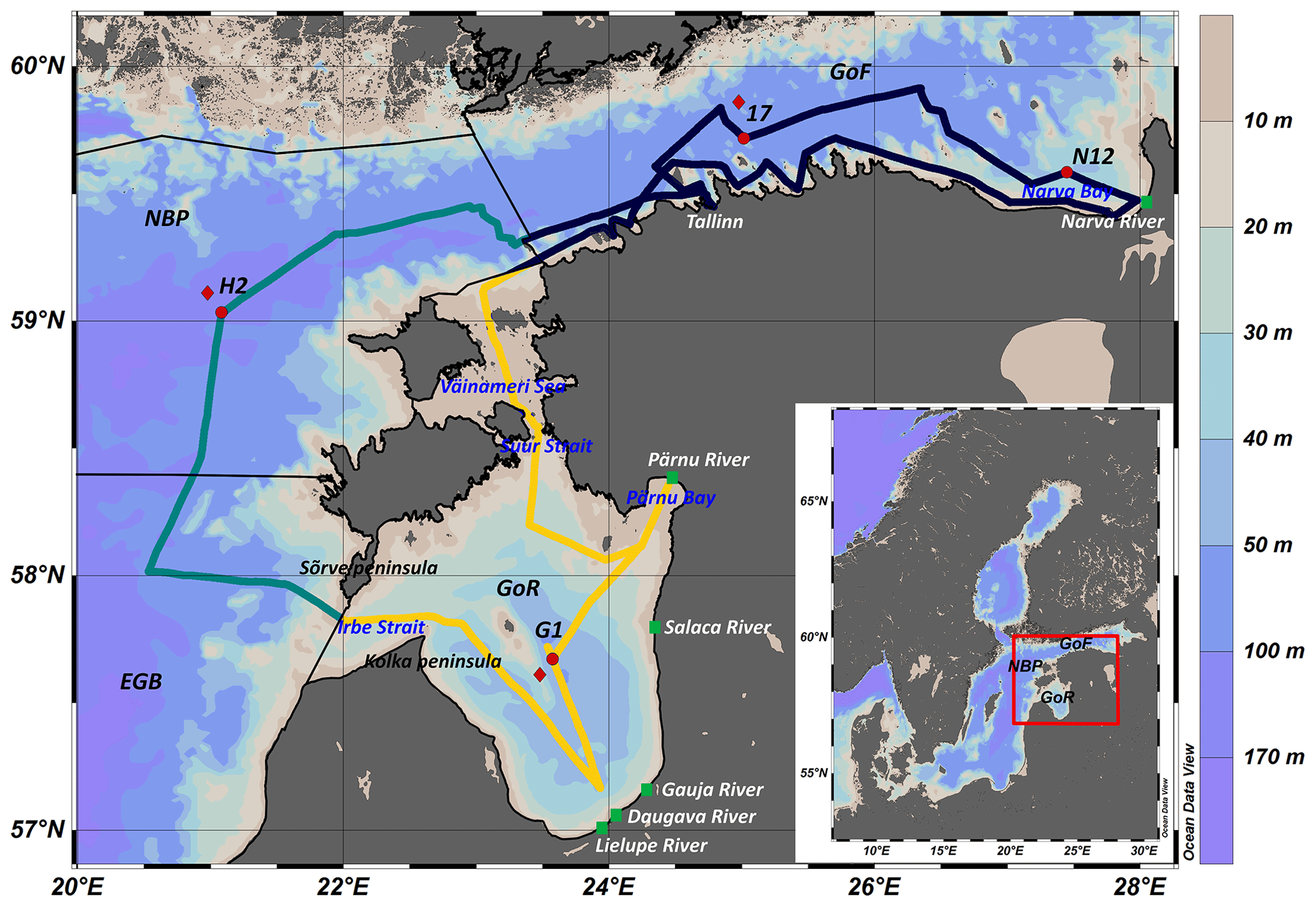
Figure 1 Map of the study area with bottom topography. GoF stands for Gulf of Finland (blue cruise track), NBP stands for Northern Baltic Proper (green), and GoR stands for Gulf of Riga (yellow) (according to HELCOM sub-basin division, marked with black lines). Green-filled squares denote river runoffs. Red-filled circles represent the locations of the most characteristic stations of the sub-basins. Red-filled diamonds denote the closest meteorological ERA5 data grid points to the most characteristic stations of each sub-basin. This map was generated using Ocean Data View (Reiner Schlitzer, Ocean Data View, https://odv.awi.de/, last access: 28 June 2023, 2022).

2 Study area

The Baltic Sea is a brackish, semi-enclosed sea in northern Europe. High freshwater runoff from the catchment area and sporadic saline water inflows from the North Sea maintain horizontal gradients and vertical stratification (e.g. Leppäranta and Myrberg, 2009). A quasi-permanent halocline exists at depths of 60–70 m in the deeper basins, and a seasonal thermocline develops at depths of 10–20 m from spring to autumn. The present study covers the following Baltic Sea sub-basins (Fig. 1): the NBP (we also include within this a small fraction of the eastern Gotland Basin), the GoF, and the GoR.

The Northern Baltic Proper is the deepest sub-basin, with a maximum depth of about 200 m and very variable topography and coastline. The quasi-permanent halocline separates oxygenated waters in the upper layers and hypoxic and anoxic waters below the halocline. However, no quasi-stationary horizontal gradients of environmental parameters exist in the surface layer. The general circulation pattern in the surface layer is considered mostly cyclonic (e.g. Placke et al., 2018). However, the presence of the northward boundary current along the eastern coasts depends on local wind patterns, and as a consequence downwelling and (less often) upwelling events and associated mesoscale currents may occur (Liblik et al., 2022).

The Gulf of Finland is an elongated basin (length about 400 km, width varies between 48 and 135 km) with a mean depth of 37 m (depths > 100 m in the western gulf). Due to the direct connection to the NBP in the west and the largest freshwater discharge in the eastern end (Neva River), surface layer salinity decreases from about 6–7 g kg⁻¹ at the entrance area to < 2 g kg⁻¹ in the easternmost area (e.g. Alenius et al., 1998). During winter, the waterbody is mixed fully in the shallower areas and down to the depth of the quasi-permanent halocline in deeper areas (Alenius et al., 2003). Hypoxic conditions are often observed below the halocline in the deeper areas (e.g. Stoicescu et al., 2019). General circulation in the surface layer is classically considered to be cyclonic (Andrejev et al., 2004) but could be seasonally variable (Maljutenko and Raudsepp, 2019). Energetic mesoscale features, i.e. eddies, fronts, upwelling events, etc. (Pavelson, 2005; Lips et al., 2016a; Kikas and Lips, 2016), may frequently occur. The largest freshwater source along the research vessel (R/V) track analysed in the present study is the Narva River in the south-eastern GoF. Depending on the seasonally varying runoff and local wind conditions, the river water spreads towards the open sea or along the coast and mixes with the gulf water masses (Laanearu and Lips, 2003).

The Gulf of Riga is a semi-enclosed shallow basin with a mean depth of 26 m (Ojaveer, 1995), and the maximum depth of the central basin of 56 m (Stiebrins and Väling, 1996). Freshwater discharge originates mostly from five larger rivers (Daugava, Lielupe, Gauja, Pärnu, and Salaca) in the southern and eastern parts of the gulf (Yurkovskis et al., 1993). Saltier waters from the Baltic Proper enter the gulf via the Irbe Strait in the west (about 70 %–80 % of water exchange) and the Suur Strait in the north (Astok et al., 1999). The whole-basin circulation in the surface layer depends on the prevailing wind pattern, which is mostly cyclonic but anti-cyclonic in summer (Lips et al., 2016b). Anti-cyclonic circulation could also prevail in the southern gulf, connected to the discharges from the Daugava and Lielupe rivers (Soosaar et al., 2016). Due to the shallowness of the basin, the water column is fully mixed in autumn–winter. Thermal stratification starts to develop in April and decays in October–December, depending on the water depth and yearly variable meteorological conditions (Skudra and Lips, 2017; Stoicescu et al., 2022). Near-bottom seasonal hypoxia can be observed in the deeper areas of the central gulf (Stoicescu et al., 2022).

The research vessel track reached the southern gulf close to the largest river discharges (Daugava and Lielupe) and Pärnu Bay, which is shallow and under the influence of the Pärnu River discharge. The measurements were also conducted in the Väinameri Sea, which is the shallow and sheltered sea area (average depth of 5–10 m) between the mainland and the western Estonian islands.

3 Material and methods

The spatial variability and seasonal dynamics of CO₂ and CH₄ in three sub-basins of the north-eastern Baltic Sea in the study year are characterized here. The results are analysed considering the background meteorological and hydrographic conditions, e.g. upper mixed layer (UML) temperature and depth, bottom depth vs. UML depth, fronts and upwelling events, and seasonal and spatial patterns of Chl a distribution in the surface layer. CO₂ and CH₄ fluxes are also estimated for all studied areas. Measurement approaches, additional data sources, and calculation methods are described below.

3.1 Meteorological information

Meteorological conditions were evaluated by ERA5 comprehensive reanalysis data (from Copernicus Climate Data Store; Hersbach et al., 2019). Surface net solar radiation, air temperature at 2 m above the sea surface, and winds at 10 m above the sea surface were extracted for the positions closest to the monitoring stations 17, G1, and H2 in the GoF, GoR, and NBP, respectively (see Fig. 1). For the comparison of the study year (2018) and the long-term (1979–2018) meteorological conditions, ERA5 data at station NBP were used. Monthly average reanalysis values in 2018 are presented against the long-term monthly averages and variability, characterized by standard deviations and minimum and maximum values. Average wind vectors and wind roses were calculated for the selected stations in the GoF, GoR, and NBP (Fig. 1) for the cruise periods using 2018 hourly reanalysis data. The presented wind characteristics during the cruises represent 7 d periods ending at the cruise termination date, i.e. periods containing 1–2 d before the cruise up to its end.

3.2 Continuous surface water measurements aboard R/V Salme

The measurements were conducted using a flow-through system (Ferrybox) onboard R/V Salme during six monitoring cruises in 2018: on 8–12 January, 16–20 April, 28 May–2 June, 9–13 July, 22–27 August, and 22–28 October. The Ferrybox by Go-systemelektronik was equipped with an SBE38 sensor for temperature, an SBE45 MicroTSG sensor for temperature and conductivity, WetLabs ECO FL and Turner Design Cyclops-7 sensors for chlorophyll a fluorescence, and a digital optode by PONSEL for dissolved oxygen measurements. The Ferrybox water intake was located at a depth of 2 m. The sampling interval was 1 min, corresponding to a nominal spatial resolution of about 250 m while the vessel was moving with its normal cruising speed of 8–9 kn.

The Ferrybox was supplemented with the equipment for trace gas (CO₂ and CH₄) measurements using an equilibrator setup. During the first cruise in January, a LI-COR 6262 ${\mathrm{CO}}_{\mathrm{2}}/{\mathrm{H}}_{\mathrm{2}}\mathrm{O}$ instrument coupled to the headspace of a glass equilibrator (similar to Gülzow et al., 2011) was used. During the other cruises, the setup was similar to the MESS presented in Sabbaghzadeh et al. (2021) using a Los Gatos Research ${\mathrm{CH}}_{\mathrm{4}}/{\mathrm{CO}}_{\mathrm{2}}$ analyser but with a lower water flow of around 2.5–4.5 L min⁻¹. In July and October, the e-folding response times of the setup were exemplarily determined to be 720 and 790 s for CH₄ and 35 and 52 s for CO₂; the lower values in July illustrate the influence of higher water temperature (ca. 18 °C vs. 12.5 °C) and higher water flow (ca. 3.6 L min⁻¹ vs. 3.1 L min⁻¹). Apart from January, an additional Microx 4 oxygen meter PSt7 optode measured dissolved oxygen in the water supply line of the equilibrator.

Atmospheric pressure was measured during the entire cruise, and measurements of atmospheric CO₂ and CH₄ (as mole fractions in ppm or ppb) were performed one to two times per cruise. For this, the gas supply of the trace gas analyser was switched from the equilibrator to a long tubing used to sample air on the windward side of the upper deck.

The data series contain surface layer temperature, salinity, chlorophyll a concentration (Chl a), partial pressure of CO₂ (pCO₂), dissolved oxygen concentration, and concentration of CH₄ (cCH₄) with a spatial resolution of about 250 m along the cruise tracks with a length of about 1500 km each, covering three Baltic Sea sub-basins.

3.3 Quality assurance and processing of continuous flow-through data

A two-step calibration procedure was followed for the Ferrybox Chl a fluorescence data. First, a linear regression was found between Chl a fluorescence data from the conductivity–temperature–depth (CTD) (Ocean Seven 320plus, Idronaut s.r.l., with Seapoint fluorometer) and Chl a concentrations determined in the laboratory from the water samples collected at respective stations and depths. Chl a concentration in the laboratory was determined optically by spectrophotometry (HELCOM, 2017). Afterwards, a linear regression between the calibrated Chl a data from CTD at 2 m depth and Ferrybox Chl a fluorescence data was found. This calibration procedure was performed separately for each cruise.

The same two-step calibration procedure was used for dissolved oxygen measurements during the cruises in January and April. Dissolved oxygen concentrations from water samples were determined electrochemically using a dissolved oxygen meter (OX 400 1 DO analyser; WWR International, LCC) and also taking into account a salinity correction. For other cruises, the Microx 4 oxygen meter PSt7 optode data were used. Oxygen partial pressures (pO₂) from the PSt7 optode were post-calibrated using discrete sample measurements conducted at 1 m depth at monitoring stations. The procedure was followed separately for each cruise, assuming that the first and last discrete measurements were representative of the start and end of each cruise.

Measured CO₂ and CH₄ mole fractions (xCO${}_{\mathrm{2}}/x$CH₄) were post-calibrated using a near-atmospheric standard gas (398.49 ppm CO₂, 1.91 ppm CH₄, matrix: ambient air). These target measurements were performed at the beginning and end of each cruise and almost every day at sea to achieve a drift correction if necessary. Measured xCO₂ and xCH₄ were converted into dry-air values based on water mole fractions measured by the same instrument. From these, the partial pressures (pCO${}_{\mathrm{2}}/p$CH₄) were calculated assuming 100 % humidity in the equilibrator headspace (water vapour pressure by Weiss and Price, 1980). The pCO₂ was temperature-corrected to account for water warming from the inlet to the equilibrator (Takahashi et al., 1993). CH₄ partial pressure data were converted to concentration (cCH₄) using the solubility constants given in Wiesenburg and Guinasso (1979). All equilibrator data were averaged using a 1 min rolling mean to match the temporal resolution of other Ferrybox parameters.

Despite the fact that we actually recorded mole fractions (xCO₂ and xCH₄), we report our CO₂ data as pCO₂ and CH₄ data as cCH₄, considering that these units are usually reported in studies addressing the respective gases. Accordingly, the atmospheric data were displayed as atmospheric partial pressure for CO₂ or saturation concentration calculated from temperature and salinity for CH₄.

Surface flow-through pCO₂ and cCH₄ data recorded at the monitoring stations were excluded using a speed of the vessel of less than 0.6 kn as the criterion. This was necessary because during profiling and water sampling the sampling device or ship propulsion could bring up sub-surface water, which caused artificial spikes in pCO₂ and cCH₄ signals.

3.4 CTD profiles and upper mixed layer depth

Vertical profiles of temperature, salinity, Chl a fluorescence, and dissolved oxygen were recorded at the monitoring stations using the CTD probe (Ocean Seven 320plus; Idronaut s.r.l). Salinity and the density anomaly are shown as absolute salinity (g kg⁻¹) and sigma-0 (kg m⁻³), respectively, and were calculated using the TEOS-10 equation of state (IOC et al., 2010). The depth of the UML was determined from the CTD profiles at the monitoring stations to evaluate whether vertical mixing reached all the way down to the seabed. It was done by comparing the UML depth with the water depth along the ship track adjacent to each station. The UML depth was defined according to Liblik and Lips (2012) as the minimum depth, where ${\mathit{\rho }}_z-{\mathit{\rho }}_{\mathrm{3}}>\mathrm{0.25}$ kg m⁻³, where ρ_z is the density anomaly at depth z and ρ₃ at a depth of 3 m.

3.5 Air–sea CO₂ and CH₄ flux calculations

Air–sea gas exchange calculations were performed using the FluxEngine toolbox. The FluxEngine toolbox is an open-source software package described in more detail by Shutler et al. (2016) and Holding et al. (2019).

The CO₂ fluxes were calculated using a rapid model approach (Woolf et al., 2016) implemented into the FluxEngine toolbox:

$$\begin{array}{}\text{(1)}& F=k\left({\mathit{\alpha }}_{\mathrm{W}}p{\mathrm{CO}}_{{\mathrm{2}}_{\mathrm{W}}}-{\mathit{\alpha }}_{\mathrm{A}}p{\mathrm{CO}}_{{\mathrm{2}}_{\mathrm{A}}}\right),\end{array}$$

where F (g C m⁻² d⁻¹) denotes the flux across the interface, k the gas transfer velocity, α the solubility of gas in the subsurface water and the water surface (subscripts W and A, respectively) and pCO₂ partial pressure of CO₂ in the sea surface water and atmosphere (subscripts W and A, respectively).

Methane fluxes were calculated using the same approach as for CO₂ fluxes:

$$\begin{array}{}\text{(2)}& F=k\left(c{\mathrm{CH}}_{{\mathrm{4}}_{\mathrm{W}}}-c{\mathrm{CH}}_{{\mathrm{4}}_{\mathrm{A}}}\right),\end{array}$$

where cCH₄ is concentration of CH₄ in the surface seawater and atmosphere (subscripts W and A, respectively).

In order to accurately describe the fluxes and the carbon budget, it is essential to include relevant processes to the air–sea CO₂ and CH₄ flux parameterization. Nightingale et al. (2000) was used for the gas transfer velocity parameterization for both CO₂ and CH₄ in our study. The sensitivity analysis of the gas transfer velocity in the Baltic Sea (Gutiérrez-Loza et al., 2021) used different parameterizations of the gas transfer velocity to evaluate the effect of other relevant processes in addition to wind speed on the net CO₂ flux at regional and sub-regional scales. In the Estonian sea area, they observed negligible differences in the average net CO₂ flux when using the different gas transfer parameterizations relative to the wind-based parameterization:

$$\begin{array}{}\text{(3)}& k=\left(\mathrm{0.222}{U}_{\mathrm{10}}^{\mathrm{2}}+\mathrm{0.333}{U}_{\mathrm{10}}\right)\sqrt{\mathrm{600}/\mathit{Sc}},\end{array}$$

where U₁₀ is the wind speed at 10 m above the sea surface and Sc is the Schmidt number. The Schmidt number parameterization was based on Wanninkhof (2014).

4 Results

4.1 Meteorological conditions

Meteorological conditions in the Baltic Sea area in 2018 were characterized by warmer than long-term average air and sea surface temperatures (Hoy et al., 2020; Humborg et al., 2019). Net solar radiation was above the average seasonal curve from February to September, with the maximum positive deviation in May (Fig. 2). In accordance with the latter, the monthly mean air temperature exceeded the long-term average from April until the end of the year. Except for June, the monthly mean wind speed in the spring and summer of 2018 was lower than the long-term average. All these meteorological parameters predict that the sea surface temperature should have been higher and seasonal vertical stratification stronger than on average due to the increased positive buoyancy flux and weak wind-induced mixing.

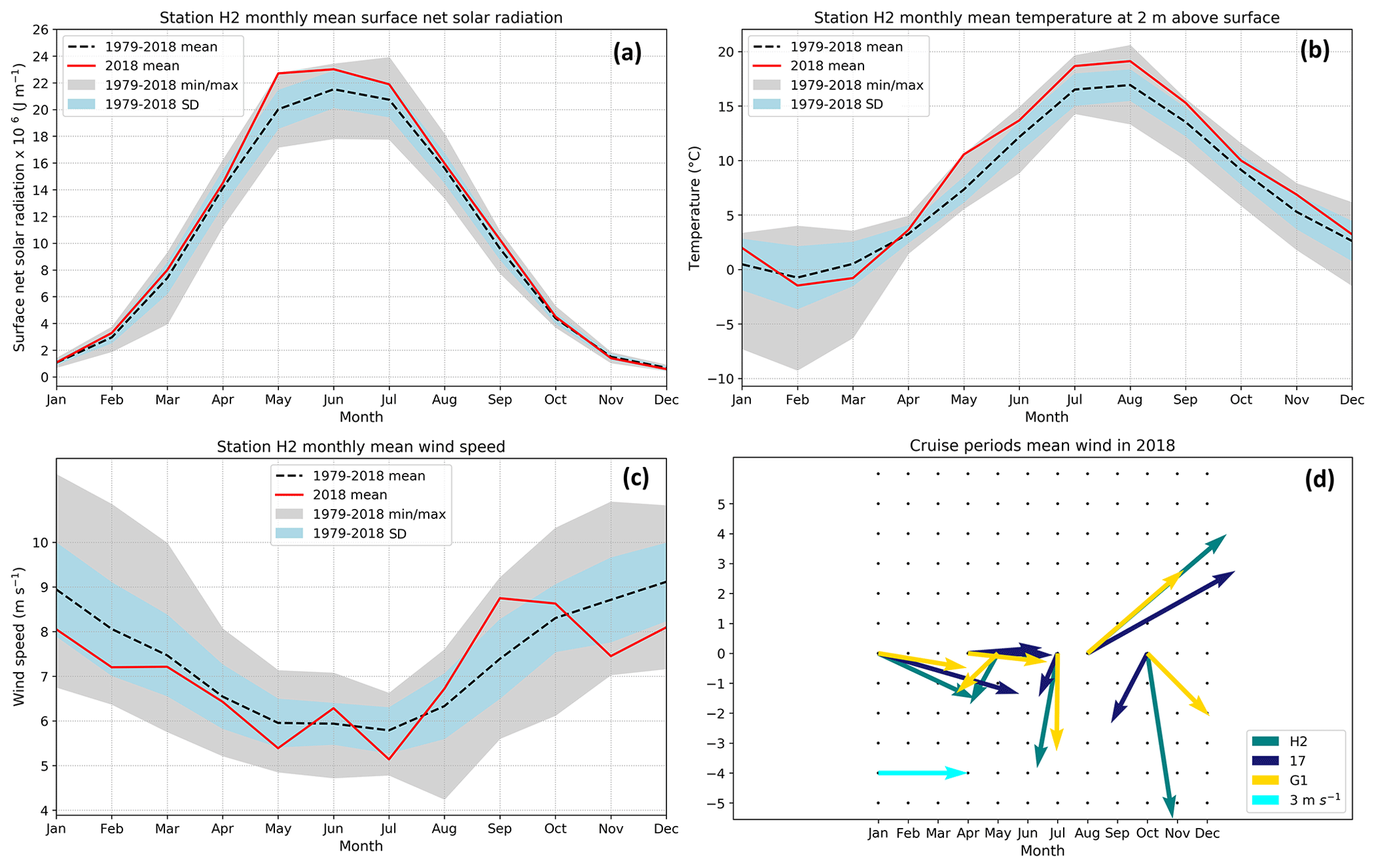
Figure 2 Monthly average (a) surface net solar radiation, (b) air temperature, and (c) wind speed in 2018 (red line) compared with the long-term averages (dashed black line), standard deviations (blue area), and minimum–maximum values (grey area) in the NBP (station H2) for the period 1979–2018. (d) Cruise period average wind vectors in the NBP (H2, green), GoF (17, blue), and GoR (G1, yellow). See Fig. 1 for the locations of stations and model grid points for data extraction.

The winds from west and south-west prevailed during and before the cruises in January, April, and August (Fig. 2), which is in accordance with the general airflow in the study area. During the cruises in July and October, the wind direction was generally from the north or north-east, while weak winds from the same direction prevailed in May–June. Note that the northerly and north-easterly winds in July and October were favourable for the upwelling development along the south-western coast of the Gulf of Finland and the eastern coasts in the Northern Baltic Proper.

The variability in wind speed and direction between the three basins and within the cruise periods is presented by the wind roses (see Fig. 3, where wind roses for three cruise periods with larger wind forcing and spatial variability are presented). The winds were mostly from one direction during the cruise in August, and a wider spread was characteristic for the cruise periods in July and October. In July, mostly two directions prevailed: easterly winds, which could cause upwelling events along the entire southern coast of the Gulf of Finland, and north-westerly winds, which are upwelling favourable for the eastern coasts of the NBP. In October, the spread of directions was the largest, but the strongest winds with speeds exceeding 15 m s⁻¹ in the GoF and NBP were from the north-east. In the GoR, wind speeds were generally lower than in the other two basins.

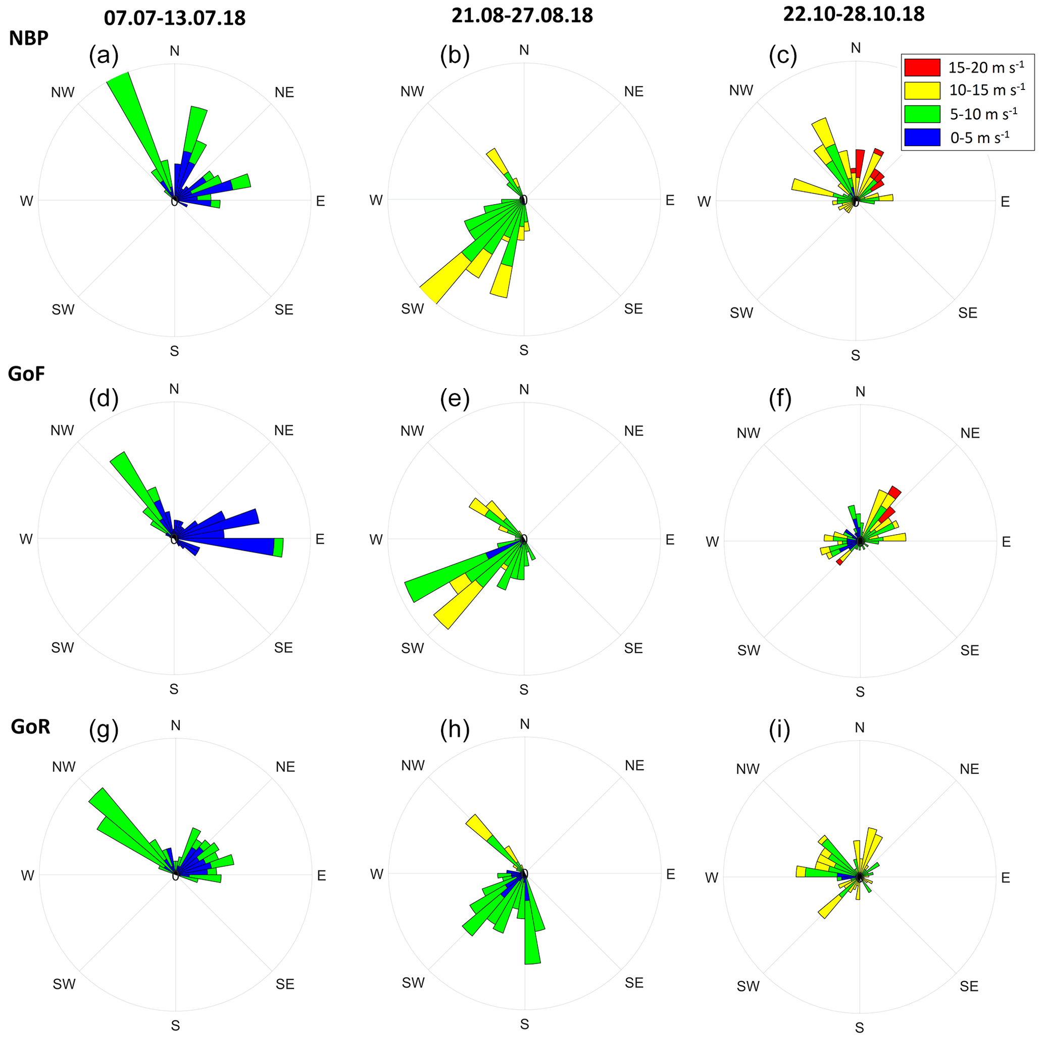
Figure 3 Cruise period wind roses in July (a, d, g), August (b, e, h), and October (c, f, i) 2018 in the NBP (a, b, c), GoF (d, e, f), and GoR (g, h, i) based on the hourly ERA5 data extracted from a grid point close to the monitoring stations H2, 17, and G1, respectively (see locations in Fig. 1). The radial axis maximum is 30 (out of 168).

4.2 Spatial variability

Surface water pCO₂ and cCH₄ distributions along the R/V track show larger spatial variability in the GoR and GoF than in the NBP for all six cruises (Figs. 4–9). Although the general seasonal pCO₂ course is evident, pCO₂ locally exceeded the atmospheric equilibrium level also during the cruises in April, May, and August. The latter is mostly valid for the GoR, but it is also valid for the GoF in August. cCH₄ was oversaturated in the surface layer during the whole study period, with prominent local peaks of cCH₄ in the GoR and GoF.

In January (Fig. 4), surface water pCO₂ along the cruise track (Fig. 4c) did not show remarkable regional differences. Values fluctuated within the range of 425–550 µatm and were oversaturated in all monitored areas. In almost all areas, the water column was well mixed down to the seabed or permanent halocline. Note that, in contrast to the other cruises, the vessel did not visit mouth areas of the rivers (neither in the GoR nor in the GoF), and cCH₄ was not measured in January.

Figure 4 January monitoring cruise (8–12 January). The trajectory is shown on the map, and in panel (a) the UML depth (light blue bars) and the water column extent below the UML (dark blue bars) are shown; vertical dashed grey lines indicate the locations of monitoring stations, while the locations of the most characteristic stations of the sub-basins are denoted with red dots. (b) Spatial variability of temperature (left y axis) and salinity (right y axis); (c) CO₂ partial pressure (left y axis) and relative saturation (right y axis); and (d) Chl a (left y axis), dissolved oxygen concentration (left y axis), and saturation (right y axis) are also shown. The x axis denotes the distance (in km) from the start of the monitoring cruise (Tallinn). The map was generated using Ocean Data View (Reiner Schlitzer, Ocean Data View, https://odv.awi.de/, last access: 14 February 2023, 2022).

The cruise in April (Fig. 5) mapped pCO₂ and cCH₄ distributions in the period of the onset of seasonal stratification and spring bloom in different development phases. The surface water pCO₂ (Fig. 5c) was mostly below the atmospheric partial pressure but reached equilibrium with the atmosphere in the western and central GoR. Low Chl a and oxygen concentrations indicate that the spring bloom was still in its initial phase in this area (Fig. 5d). In addition, the water column was mixed almost down to the seabed in this sea area. The pCO₂ values were clearly lower in the eastern part of the open GoR, the shallow Pärnu Bay, and the Väinameri Sea. These pCO₂ minima (down to 60 µatm) were associated with increased temperature and the highest Chl a and oxygen concentrations in these areas, while the influence of the Pärnu River was visible via a local peak in the pCO₂ (up to 397 µatm).

Figure 5 April monitoring cruise (16–20 April). The trajectory is shown on the map, and in panel (a) the UML depth (light blue bars) and the water column extent below the UML (dark blue bars) are shown; vertical dashed grey lines indicate the locations of monitoring stations, while the locations of the most characteristic stations of the sub-basins are denoted with red dots. (b) Spatial variability of temperature (left y axis) and salinity (right y axis); (c) CO₂ partial pressure (left y axis) and relative saturation (right y axis); (d) Chl a (left y axis), dissolved oxygen concentration (left y axis), and saturation (right y axis); and (e) CH₄ concentration (left y axis) and relative saturation (right y axis) are also shown. The x axis denotes the distance (in km) from the start of the monitoring cruise (Tallinn). The map was generated using Ocean Data View (Reiner Schlitzer, Ocean Data View, https://odv.awi.de/, last access: 14 February 2023, 2022).

From the western GoF towards the central GoF, a Chl a increase from < 9 to 15 mg m⁻³ was accompanied by slightly higher oxygen and lower pCO₂ values (about 130 µatm). Although high Chl a concentrations up to 16 mg m⁻³ were mapped along the south-eastern coast of the GoF, pCO₂ values in this area remained on a higher level (around 250 µatm) than in other regions with a similar surface layer Chl a content. Note that the water column along the coast was well mixed down to the seabed, except close to the Narva River mouth. Elevated cCH₄ was measured, similar to the pCO₂ distribution, in the western and central GoR (27–37 nmol L⁻¹) and in Pärnu Bay close to the mouth of the Pärnu River (40 nmol L⁻¹). Elevated cCH₄ was also measured along the south-western coast of the GoF (26 nmol L⁻¹; marked as SW GoF in Fig. 5e), where the water column was mixed down to the seabed, and close to the mouth of the Narva River (up to 30 nmol L⁻¹). The direct influence of the Pärnu and Narva rivers was expressed by the cCH₄ peaks.

The cruise at the end of May and beginning of June (Fig. 6) coincided with the phytoplankton summer minimum, while the water column was characterized by unusually high sea surface temperatures (13–18 °C; Fig. 6b) and a shallow upper mixed layer (Fig. 6a, on average < 6 m in the GoR and 8 m in the central GoF). The pCO₂ values had decreased to the minimum along most of the ship track, varying mostly between 50 and 100 µatm, while moderately higher (reaching 200 µatm) than background pCO₂ values were registered in the NBP–GoR transition area, the Irbe Strait. CO₂ oversaturation was locally recorded in the shallowest areas of the GoR – Pärnu Bay and the Väinameri Sea. In Narva Bay, no distinct Narva River impact was registered. Local cCH₄ maxima were observed in the shallow bays of the southern and south-western GoF (> 80 nmol L⁻¹) and in the Irbe Strait close to the Kolka Peninsula (> 35 nmol L⁻¹). Only slightly higher than background cCH₄ values were measured in the southern GoR close to the mouths of the largest rivers – the Daugava and Lielupe. In contrast, an extensive peak in cCH₄ was registered in the shallow Pärnu Bay close to the Pärnu River (maximum measured concentration was 232 nmol L⁻¹). Local maxima in the shallow Väinameri Sea increased to notable peaks along the south-western coast of the GoF. Local maxima of 33 nmol L⁻¹ in Narva Bay were likely due to the influence of the Narva River.

Figure 6 End of May monitoring cruise (28 May–2 June). The trajectory is shown on the map, and in panel (a) the UML depth (light blue bars) and the water column extent below the UML (dark blue bars) are shown; vertical dashed grey lines indicate the locations of monitoring stations, while the locations of the most characteristic stations of the sub-basins are denoted with red dots. (b) Spatial variability of temperature (left y axis) and salinity (right y axis); (c) CO₂ partial pressure (left y axis) and relative saturation (right y axis); (d) Chl a (left y axis), dissolved oxygen concentration (left y axis), and saturation (right y axis); and (e) CH₄ concentration (left y axis) and relative saturation (right y axis) are also shown. The x axis denotes the distance (in km) from the start of the monitoring cruise (Tallinn). In May, the cCH₄ signal in the river estuaries was extreme in comparison with the rest of the data, and this signal was cut here to 100 nmol L⁻¹ to properly display the structure within low-concentration areas. Note the different scale for temperature in comparison with January and April (Fig. 4 and 5, respectively). The map was generated using Ocean Data View (Reiner Schlitzer, Ocean Data View, https://odv.awi.de/, last access: 14 February 2023, 2022).

In mid-July (Fig. 7), the surface waters were undersaturated in CO₂ along the entire ship track (Fig. 7c; note that the vessel did not visit the mouth areas of the Pärnu and Narva rivers). The UML has slightly deepened in the GoR (8 m) but was the shallowest in the offshore GoF (< 7 m). Higher than 5 mg m⁻³ Chl a concentrations were observed in the offshore areas of NBP, the north-eastern GoR, and the central GoF, probably due to the development of the summer bloom. Elevated pCO₂ values were recorded in parts of the NBP offshore areas (330 µatm) and the coastal sea area in the Irbe Strait (310 µatm) and the Väinameri Sea (355 µatm). Local maxima of cCH₄ up to 43 nmol L⁻¹ were observed in the shallow bays of the southern and south-western GoF, including the transition area into the GoF. In comparison with the cruise at the end of May, in July a relatively low cCH₄ peak (14 nmol L⁻¹) was observed in the Irbe Strait, and the influence of large rivers in the southern GoR was almost not detectable.

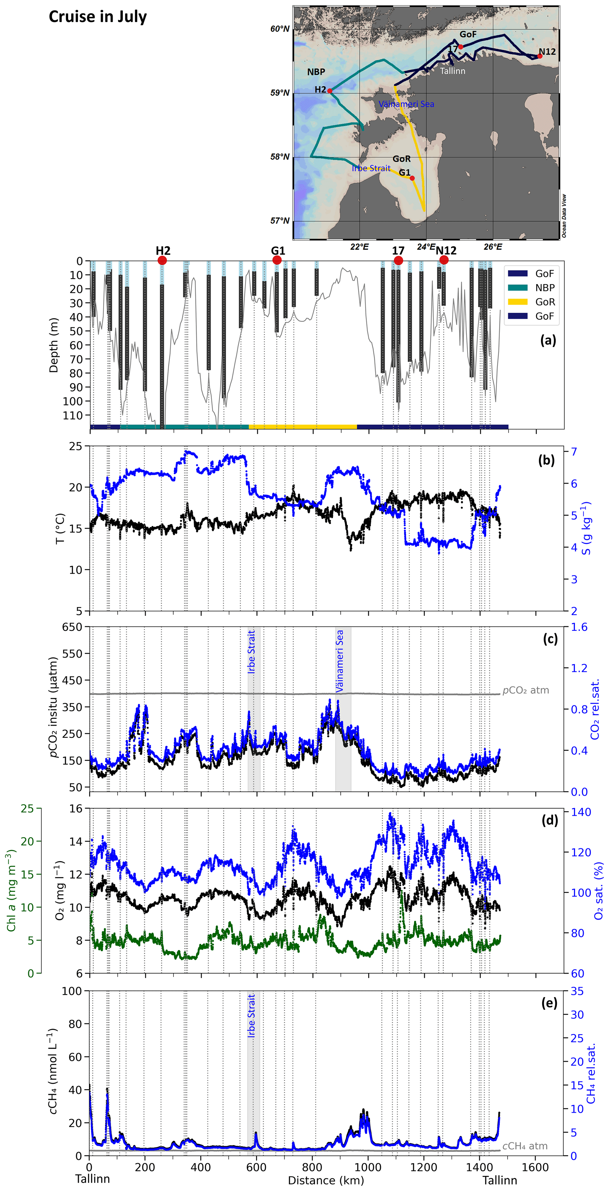
Figure 7 July monitoring cruise (9–13 July). The trajectory is shown on the map, and in panel (a) the UML depth (light blue bars) and the water column extent below the UML (dark blue bars) are shown; vertical dashed grey lines indicate the locations of monitoring stations, while the locations of the most characteristic stations of the sub-basins are denoted with red dots. (b) Spatial variability of temperature (left y axis) and salinity (right y axis); (c) CO₂ partial pressure (left y axis) and relative saturation (right y axis); (d) Chl a (left y axis), dissolved oxygen concentration (left y axis), and saturation (right y axis); and (e) CH₄ concentration (left y axis) and relative saturation (right y axis) are also shown. The x axis denotes the distance (in km) from the start of the monitoring cruise (Tallinn). The map was generated using Ocean Data View (Reiner Schlitzer, Ocean Data View, https://odv.awi.de/, last access: 14 February 2023, 2022).

In August (Fig. 8), CO₂ varied around the saturation level. The surface waters were undersaturated in CO₂ in most areas of the GoF except Narva Bay, where the water column was well-mixed down to the seabed; oversaturated in the Väinameri Sea and Pärnu Bay; and undersaturated in the NBP (Fig. 8c). These higher pCO₂ values were characteristic for the shallow areas and could be only partly related to the river discharge (as in Narva Bay and Pärnu Bay). A distinct local maximum in pCO₂ of 460 µatm was related to the salinity front in the Irbe Strait, as also observed earlier. Local cCH₄ maxima were observed in the shallow bays of the southern and south-western GoF and along the south-eastern coast of Narva Bay. Locally, well-pronounced cCH₄ peaks with a maximum concentration of 177 nmol L⁻¹ were also observed in the Väinameri Sea and Pärnu Bay. The increase in cCH₄ in the Irbe Strait (38 nmol L⁻¹) was comparable with the cCH₄ peak at the end of May cruise.

Figure 8 August monitoring cruise (22–27 August). The trajectory is shown on the map, and in panel (a) the UML depth (light blue bars) and the water column extent below the UML (dark blue bars) are shown; vertical dashed grey lines indicate the locations of monitoring stations, while the locations of the most characteristic stations of the sub-basins are denoted with red dots. (b) Spatial variability of temperature (left y axis) and salinity (right y axis); (c) CO₂ partial pressure (left y axis) and relative saturation (right y axis); (d) Chl a (left y axis), dissolved oxygen concentration (left y axis), and saturation (right y axis); and (e) CH₄ concentration (left y axis) and relative saturation (right y axis) are also shown. The x axis denotes the distance (in km) from the start of the monitoring cruise (Tallinn). In August, cCH₄ signals in the river estuaries and coastal areas were extreme in comparison with the rest of the data, and these signals were cut here to 100 nmol L⁻¹ to properly display the structure within low-concentration areas. The map was generated using Ocean Data View (Reiner Schlitzer, Ocean Data View, https://odv.awi.de/, last access: 14 February 2023, 2022).

In October (Fig. 9), surface waters were oversaturated in CO₂ almost along the entire ship track (Fig. 9c). Like during the August cruise, pCO₂ values were lower in the NBP (varying between 400 and 480 µatm) than in the GoF and GoR (varying up to 600 µatm). In contrast to the summer cruises, higher pCO₂ values were characteristic for the offshore areas in the GoR, and lower values were present in the shallow coastal sea areas – Pärnu Bay and the Väinameri Sea. The pCO₂ values exceeding 1200 µatm were registered in connection to an upwelling event in the SW GoF caused by the strong north-westerly winds before and during the cruise. Peaks in cCH₄ up to 80 nmol L⁻¹ were registered in the shallow bays along the southern coast of the GoF. In the Irbe Strait, cCH₄ increased up to 15 nmol L⁻¹ in October. A clear cCH₄ peak of 62 nmol L⁻¹ was detected in Pärnu Bay, probably influenced by the Pärnu River discharge. Local maxima in the Väinameri Sea increased to an extensive broad peak (69 nmol L⁻¹) in the upwelling waters in the SW GoF.

Figure 9 October monitoring cruise (22–28 October). The trajectory is shown on the map, and in panel (a) the UML depth (light blue bars) and the water column extent below the UML (dark blue bars) are shown; vertical dashed grey lines indicate the locations of monitoring stations, while the locations of the most characteristic stations of the sub-basins are denoted with red dots. (b) Spatial variability of temperature (left y axis) and salinity (right y axis); (c) CO₂ partial pressure (left y axis) and relative saturation (right y axis); (d) Chl a (left y axis), dissolved oxygen concentration (left y axis), and saturation (right y axis); and (e) CH₄ concentration (left y axis) and relative saturation (right y axis) are also shown. The x axis denotes the distance (in km) from the start of the monitoring cruise (Tallinn). In October, cCH₄ signal in the coastal areas was extreme in comparison with the rest of the data, and this signal was cut here to 100 nmol L⁻¹ to properly display the structure within low-concentration areas. Note the different scales for CO₂ partial pressure and relative saturation in comparison with the rest of the cruises. The map was generated using Ocean Data View (Reiner Schlitzer, Ocean Data View, https://odv.awi.de/, last access: 14 February 2023, 2022).

4.3 Seasonal variability

Seasonal variability of pCO₂ in 2018 (Fig. 10d) follows the general seasonal course in all analysed sub-basins (Table 1), with oversaturation in autumn–winter (average relative CO₂ saturation 1.2) and undersaturation in spring–summer (average relative CO₂ saturation 0.5). The pCO₂ decrease in spring coincides with the highest Chl a and dissolved oxygen concentrations in April. Based on decreased Chl a concentrations from mid-April to the end of May (Fig. 10e; Table 1), the early summer minimum of phytoplankton biomass was evident. It is also at the end of May to early June when the pCO₂ seasonal minimum in all sub-basins appeared (Table 1). During midsummer, relatively high Chl a concentrations were recorded (Fig. 10e; Table 1), while dissolved oxygen concentrations stayed moderately oversaturated. The pCO₂ values increased from July on, reaching oversaturation almost everywhere along the cruise track by the October cruise. No second pCO₂ minimum during summer or relative maximum between the two usually expected minima in spring and late summer was detected.

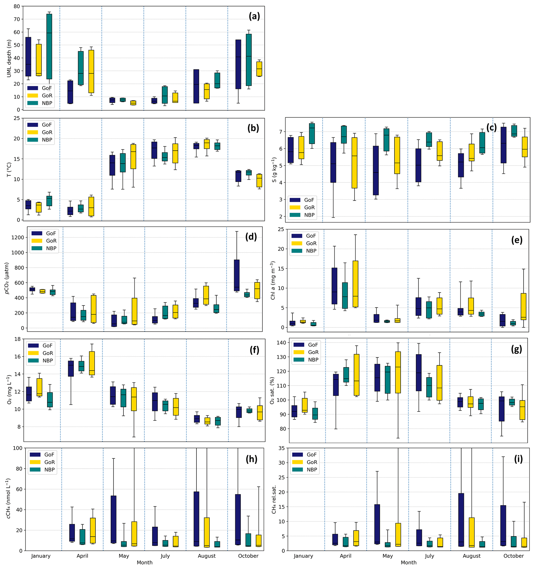
Figure 10 Median and 5th and 95th percentile values of (a) UML depth, (b) temperature, (c) salinity, (d) CO₂ partial pressure, (e) Chl a, (f) dissolved oxygen, (g) oxygen saturation, (h) CH₄ concentration, and (i) CH₄ relative saturation. Whiskers denote minimum and maximum values. In the May, August, and October cruises, cCH₄ signals in the river estuaries and coastal areas were extreme in comparison with the rest of the data, and these signals are not seen on the plot (y-axis maximum is 100 nmol L⁻¹ to properly display the pattern in low-concentration areas).

Table 1 Median and mean (value before and after the slash, respectively) values of UML depth, temperature (T), salinity (S), CO₂ partial pressure (pCO₂), Chl a, dissolved oxygen (O₂), oxygen saturation (O₂ sat.), CH₄ concentration (cCH₄), and CH₄ relative saturation (CH₄ rel.) for the Estonian sea area sub-basins in 2018.

For the evaluation of the seasonal course of surface water methane concentrations, cCH₄ median values were analysed (Fig. 10h and Table 1). In all three sub-basins, the highest median concentrations of 13.7 nmol L⁻¹ in the GoR, 11.5 nmol L⁻¹ in the GoF, and 7.6 nmol L⁻¹ in the NBP were determined in April (note we do not have winter data), after which the concentrations started to decrease. The minimum level was reached in the GoF and GoR in July (median concentrations were 7.9 and 4.5 nmol L⁻¹, respectively) and in the NBP in August (3.9 nmol L⁻¹). It was followed by an increase in concentrations by October, but the values did not yet reach the levels observed in April.

Although high cCH₄ values represent only a small part of acquired data, it is worthwhile to mark some seasonal changes in variability. The highest cCH₄ variations were observed in May, August, and October in the GoF and in April, May, and August in the GoR. It shows that although the average seasonal course in the GoF and GoR was similar to the NBP, regions existed in the GoF and GoR with locally high methane concentrations (extremes exceeding 100 nmol L⁻¹).

4.4 Estimates of the air–sea CO₂ and CH₄ fluxes

The air–sea CO₂ and CH₄ fluxes calculated for every research cruise were seasonally averaged so that winter is characterized by the cruise in January, spring by the cruises in April and May, summer by the cruises in July and August, and autumn by the cruise in October (Tables 2 and 3; Fig. 11).

Table 2 Seasonal and annual CO₂ flux estimates with standard deviations for the Estonian sub-basins and sea area in 2018.

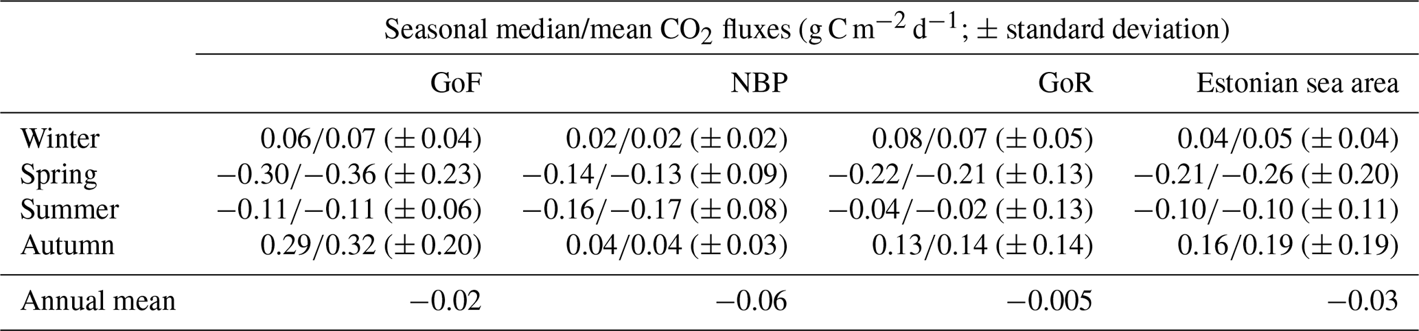
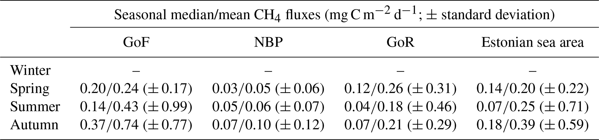
Table 3 Seasonal CH₄ flux estimates with standard deviations for the Estonian sub-basins and sea area in 2018.

The CO₂ flux estimates (Table 2) show that the Estonian sea area was a source of atmospheric CO₂ (positive flux) during winter and autumn and a sink (negative flux) during spring and summer 2018. What stands out is that the standard deviations are of the same order of magnitude as the estimated average fluxes. The observed spatial variability was larger in the GoR and GoF than in the NBP (Figs. 4–9). The annual mean flux (estimated as an arithmetic average of the four seasonal flux estimates) was −0.06 g C m⁻² d⁻¹ in the NBP, −0.02 g C m⁻² d⁻¹ in the GoF, and −0.005 g C m⁻² d⁻¹ in the GoR.

The CH₄ flux estimates (Table 3) show that the Estonian sea area was a source of atmospheric CH₄ during spring, summer, and autumn (no data for winter). Note that the standard deviations of flux estimates exceeded the resulting average fluxes during summer and autumn. As with CO₂ fluxes, the spatial variability of observed CH₄ fluxes was larger in the GoR and GoF than in the NBP (Fig. 11).

Figure 11 Seasonal median air–sea (a) CO₂ and (b) CH₄ flux estimates in the three analysed sub-basins of the north-eastern Baltic Sea in 2018. The flux is positive for the transport from the sea to the atmosphere, while negative values refer to the transport from the atmosphere to the sea.

5 Discussion

The first extensive trace gases study was conducted to describe spatial patterns and seasonal dynamics of CO₂ and CH₄ in the north-eastern Baltic Sea area. The main focus was on the southern Gulf of Finland and the Gulf of Riga, as earlier studies addressed measurements from the Baltic Proper and the western Gulf of Finland (e.g. Schneider et al., 2014; Schneider and Müller, 2018; Gülzow et al., 2013).

5.1 Patterns of variability in the southern GoF and GoR

5.1.1 pCO₂ distribution patterns

Cruises of R/V Salme covered both the offshore and the coastal areas in the GoF and GoR, with the most prominent local pCO₂ peaks in the shallow coastal sea areas. These local maxima were mostly linked to river bulges, coastal upwelling events, fronts, and vertical mixing reaching the seabed but also to phytoplankton distribution patterns influenced by meteorological and hydrographic conditions.

Rivers are the major carbon source, including dissolved inorganic carbon for the coastal ocean (Dai et al., 2022) and the Baltic Sea (Kuliński and Pempkowiak, 2011). In the GoF, the largest freshwater source along the R/V track was the Narva River (Stålnacke et al., 1999). Its influence, identified by a simultaneous local decrease in salinity and increase in pCO₂, was largest in August (Fig. 8c), when CO₂ concentrations locally exceeded saturation level, while in April and May–June, only a slight increase in pCO₂ relative to the surrounding waters was observed. In the GoR, river discharge is concentrated in the southern and eastern parts of the gulf (Yurkovskis et al., 1993). The influence of large rivers of the southern GoR was detected by a slight decrease in salinity in May–June and July, but a simultaneous increase in pCO₂ was observed only in May–June. The largest peaks, which could be linked to the river discharges, were associated with the Pärnu River, especially in April and May–June, when the background levels of pCO₂ in the adjacent regions were already low. Thus, the river waters influenced the observed pCO₂ patterns remarkably in the shallow and semi-enclosed Pärnu Bay and less in other areas.

Upwelling is the most prominent mesoscale process in the elongated GoF (Myrberg and Andrejev, 2003), where upwelling events along the southern coast are associated with north-easterly and easterly winds (Lips et al., 2009; Kikas and Lips, 2016). Winds supporting upwelling along the GoF southern coast dominated in October and also in July and late May, albeit with lower wind speed. In October, based on a comparison of salinity and temperature in the surface layer in the upwelling area and vertical profiles registered at the monitoring stations 2 d earlier, the upwelled waters mostly originated from the water layer of 65–75 m, i.e. the halocline. Most likely, the observed extreme pCO₂ values were caused by the relatively deep origin and the impact of the seabed when these waters were brought to the surface along the GoF slope.

In a case of upwelling in the Gotland Basin in July–August 2016, a very sharp increase in pCO₂ was measured, although the absolute values were lower than in our study (Jacobs et al., 2021). The authors evaluated the air–sea fluxes of CO₂ due to this upwelling event and showed that the CO₂ flux, expected to be directed from air into the sea in August, was reduced and even reversed due to upwelling. Kuss et al. (2006) have suggested that roughly 20 % of the annual CO₂ uptake in the central Arkona Sea could be balanced by CO₂ release during occasional upwelling events in the coastal areas, also considering seasonal differences in their impact. Similarly, Norman et al. (2013) estimated that upwelling events could possibly decrease the Baltic Sea's annual average CO₂ uptake by up to 25 %. In 2018, winds favouring upwelling along the northern coast of the GoF prevailed. However, we detected the upwelling events in the western GoF along the southern coast during cruises in late May and October. The highest pCO₂ values were recorded in upwelled waters in October when autumn mixing likely contributed to the vertical exchange, but it did not trigger production.

The seasonal course in pCO₂ in the surface layer is mainly controlled by the primary production in spring and summer and entrainment of waters with high pCO₂ due to remineralization processes during mixed-layer deepening in autumn (e.g. Schneider and Müller, 2018). The seasonal succession of phytoplankton, however, could be at different stages of development due to varying meteorological and hydrographic background along the 1500 km long measurement track (e.g. Seppälä and Balode, 1999; Lips et al., 2014). In April, the highest pCO₂ values, corresponding to the saturation level, observed in the parts of the GoR and GoF coincided with lower than the background Chl a and oxygen concentrations (Fig. 5c and d). The lowest pCO₂ values were recorded in shallow areas with a warm surface layer with high Chl a concentrations. It is remarkable that in areas of high pCO₂, the sea surface temperature was 1–2 °C, meaning below the temperature of the maximum density of approximately 2.5 °C, and the water column was almost fully mixed, e.g. in the western and central GoR.

Like the stratification and bloom development in spring, the upper mixed layer deepening and stratification decay could shape the pCO₂ distribution patterns in the surface layer in late summer and autumn. By the August cruise, the upper mixed layer has been deepened to almost 30 m from the values of around 10 m in July. This resulted in high pCO₂ values in shallow areas (Fig. 8c), where the mixing has reached the bottom layer. However, the areas with higher pCO₂ values during summer cruises had CO₂ levels in October lower than in the deeper areas, where the mixing reached the near-bottom layer later, leaving less time for equilibration with the atmosphere in these deeper areas.

We suggest the following processes are responsible for the observed seasonal pattern in the Väinameri Sea (northern GoR) with an average depth of 5–10 m and relatively strong gradients of oceanographic variables (Suursaar et al., 2001). In April, pCO₂ levels were lower than in the adjacent deeper areas due to a warm surface layer and an earlier start of the spring bloom since the phytoplankton mixing depth in shallow areas is determined by the bottom depth and not vertical stratification (Townsend et al., 1994). In late May and July, the highest pCO₂ values were measured at the saltier side of the salinity front in the Väinameri Sea, likely favoured by weaker vertical stratification and, consequently, stronger vertical fluxes at the denser side of the fronts (e.g. Kahru et al., 1984). In August, the higher pCO₂ values in the shallow Väinameri Sea were likely related to the vertical mixing, and in October, when oversaturation was observed almost along the entire R/V track, pCO₂ was higher in other, deeper areas where the vertical flux (due to continuing upward mixing of deep, CO₂-rich waters) was still at a higher level, while a larger fraction of the CO₂ from the near-bottom layer had already been transported away from the Väinameri Sea.

Another area where saltier Baltic Proper and fresher GoR waters meet and the front develops is the Irbe Strait, conveying most of the GoR water exchange with the NBP (Lilover et al., 1998). Locally, the lowest pCO₂ was measured in connection to the Irbe front in April, probably due to the development of vertical stratification supporting the spring bloom, while in the GoR stratification was weak, and the bloom had not started yet. Contrarily, a slight local peak of pCO₂ in July could be caused by more intense vertical transport of sub-surface waters at the front.

5.1.2 cCH₄ distribution patterns

cCH₄ was oversaturated in the surface layer during the whole study period, which is typical for the Baltic Sea (Gülzow et al., 2013), with prominent local peaks in the GoF and GoR. These peaks can be related to the same physical processes as the local maxima in pCO₂ spatial distribution. However, two major peculiarities of cCH₄ distribution can be noticed – the local maximum values were more than an order of magnitude larger than the background cCH₄ level, and these prominent maxima were confined to the shallow areas. Although these peaks were not always observed in all shallow areas, this pattern agrees with the earlier results that methane concentrations and variability are high in shallow coastal areas (Roth et al., 2022; Borges et al., 2016).

Rivers have been identified as potentially strong sources of CH₄ in the Baltic Sea (Myllykangas et al., 2020), receiving CH₄ from soils, groundwater, wetlands, and floodplains in the watershed (De Angelis and Lilley, 1987; Richey et al., 1988). In April and May, elevated cCH₄ was measured near the Narva River mouth. However, the enhanced cCH₄ was also measured along the shallow coastal sea towards the west from the Narva River mouth. Similar distribution in August, with the maximum not at the mouth area but in the west, suggests that the river discharge was transported along the coast, as it could occur during summer months (Laanearu and Lips, 2003) or the shallowness and influence of sediments was the main factor creating this cCH₄ maximum. The latter suggestion or a combination of both would be the most likely explanation, since the water column was fully mixed along the ship track in this area.

Notable cCH₄ spatial variability emerged in the shallow Pärnu Bay, while cCH₄ values only slightly higher than the background were measured in the southern GoR. The research vessel track probably did not reach the river bulges properly in the southern GoR, or their influence was not seen offshore since the riverine waters were mostly transported along the coast (e.g. Lips et al., 2016b) and an anticyclonic river bulge was not formed as suggested by a modelling study (Soosaar et al., 2016). The highest cCH₄ peaks in the Pärnu Bay were observed in May and August (approximately 200 nmol L⁻¹), while in October, the peak was not so prominent, although the river discharge was larger than in summer months. In shallow coastal areas, high methane emissions have been linked to the amount of organic matter in the sediment and water temperature (e.g. Heyer and Berger, 2000). In addition, local maxima of cCH₄ were more pronounced in Pärnu Bay in comparison with the areas close to the Narva River mouth. We suggest that this pattern is related to the shallowness and semi-enclosed shape of Pärnu Bay and not directly to the changes in the river runoff.

The seafloor in most of the shallow bays is characterized by clay and mud or mixed sediments (mud and sand; EMODnet Geology, 2023), which are potential internal sources of methane (e.g. Humborg et al., 2019). This explains why cCH₄ peaks were recorded in these shallow areas where the water column was usually mixed down to the seabed. In October, when high cCH₄ values were also measured along the relatively deep south-western GoF (Fig. 9e), these findings can be related to autumn vertical mixing and an intense upwelling event. A similar impact of upwelling has also been shown by earlier measurements in the Baltic Sea (Gülzow et al., 2013; Jacobs et al., 2021) and other coastal sea areas (e.g. Kock et al., 2008). It is noteworthy that our data show the impact of upwelling on surface CO₂ and CH₄ concentrations in fall, when upwelling was identified by salinity rather than temperature. Previous studies (Gülzow et al., 2013; Schneider et al., 2014; Jacobs et al., 2021) use the drop in sea surface temperature as an indicator for upwelling and upwelling-induced greenhouse gas fluxes, which bears the risk of underestimating the importance of upwelling for locally enhanced CO₂ and CH₄ fluxes in the Baltic in fall.

Elevated cCH₄ was almost always measured in the Väinameri Sea and can be explained by vertical mixing and resuspension of bottom sediments. Resuspension events occur due to wind mixing and waves but also due to frequently appearing strong currents in the straits (Suursaar et al., 2001; Otsmann et al., 2001). However, the detected cCH₄ peaks in the Väinameri Sea were not as strong as in Pärnu Bay, and in October a much higher cCH₄ peak was measured just outside of the Väinameri Sea in the upwelled waters in the south-western GoF (concentrations reached up to 70 nmol L⁻¹; Fig. 9e). In the Irbe Strait, local cCH₄ maxima were also frequently observed. However, their locations were different from the observed pCO₂ extrema. We suggest that the cCH₄ maxima here were also related to the shallowest spots along the vessel track (either close to the Kolka or Sõrve peninsulas) and not to the Irbe front, as was observed for the observed pCO₂ peaks.

In summary, physically disturbed organic-rich sediments, river plumes, and upwelling were identified as processes causing hot spots of methane emission. While methane from undisturbed organic-rich sediments usually does not surpass effective anaerobic and aerobic methane oxidation in the upper sediment (e.g. Knittel and Boetius, 2009), physical shear stress can lead to the release of methane from the upper sediment layer. Borges et al. (2016) suggested water depth as a proxy for methane flux over organic-rich sediments in the North Sea. Similarly, our data support the importance of processes in shallow areas for assessing the CH₄ fluxes from the Baltic (and other marginal seas) to the atmosphere.

5.2 Comparison of seasonal variability between the basins

The temporal variations in pCO₂ in the surface layer of the NBP, GoF, and GoR in 2018 generally followed the known seasonal course (Thomas and Schneider, 1999; Schneider and Müller, 2018). In the Gotland Basin, the pCO₂ seasonal amplitude between 100 and 550 µatm has been registered (Schneider and Müller, 2018). In our study, the seasonal amplitude of pCO₂ was similar in all basins, with a slightly larger range in the GoF (50–1200 µatm). This higher amplitude is likely, at least in part, a result of the lower alkalinities in the GoF, which result in a higher pCO₂ change per amount of fixed carbon (e.g. Kuliński et al., 2017). The seasonal pCO₂ minimum in all basins appeared at the end of May when surface layer Chl a concentrations were already relatively low, as a result of the cumulative nature of the imprint of primary production on the inorganic carbon system. Our data did not reveal an increase in pCO₂ between the spring bloom and the cyanobacteria bloom in midsummer, which has been reported based on measurements with a higher temporal resolution (e.g. Schneider et al., 2014).

In the GoF and the GoR, Chl a concentrations in spring (Fig. 10e, Table 1) were higher than in the NBP, which is in accordance with the elevated nutrient concentrations in the GoF and GoR (HELCOM, 2018). However, a slightly higher average pCO₂ in the GoR during spring and summer could be related to the shallowness of this basin. Higher pCO₂ in the GoF in October and January can be explained by high biomass production in spring–summer and the specific hydrographic conditions supporting vertical transport and mixing of CO₂ from the deep layers in autumn–winter and during the upwelling events, in combination with the reduced buffering due to lower alkalinity in the GoF. High concentrations of inorganic carbon in the deep layers of the GoF result from the organic matter degradation in the presence of stratification in spring and summer and the advection of deep waters from the Baltic Proper (Lehtoranta et al., 2017). In late autumn and winter, collapses of vertical stratification could occur in the GoF (Liblik et al., 2013), resulting in the vertical transport of nutrients (and inorganic carbon) from the near-bottom layer to the surface layer (Lips et al., 2017). The high pCO₂ values attributed to upwelling in October in the GoF, also characterized by the lowest surface O₂ saturation of the entire survey, confirm active transport mechanisms of deep waters with strong biogeochemical indicators of mineralization of organic matter (Fig. 9c).

Since the GoR is shallower than the GoF and without a permanent halocline, CO₂ accumulation and subsequent CO₂ flux from the GoR deep layer do not have a similar high potential in autumn–winter to that in the GoF. However, the seasonal thermocline was stronger in spring–summer 2018 than on average due to high heat flux and calm wind conditions (Stoicescu et al., 2022). A near-bottom hypoxic layer developed, and the autumn–winter mixing had not reached the seabed in the deeper central GoR yet by the cruise in October (Stoicescu et al., 2022, also Fig. 9a). This could be a reason that relatively low pCO₂ was measured in the GoR while upwelling-related high values were recorded in the south-western GoF.

In our study, the second pCO₂ minimum in summer (or an increase between two minima) was not revealed, probably due to the long interval between cruises: 5 weeks between the cruises in late May–early June and mid-July and 5 weeks between the cruises in mid-July and the end of August. Summer cyanobacterial bloom in the GoF usually starts at the end of June or early July (Lips and Lips, 2008). Based on our data from mid-July, calm wind conditions and high sea surface temperatures (median 17.7 °C, Table 1) favoured the bloom, which is also observable in an increase in Chl a concentration. Müller et al. (2021) showed that in 2018 in the eastern Gotland Basin, the production was intense from the beginning of their study period, 6 July (surface water pCO₂ was already as low as around 100 µatm), and Nodularia sp. peaked on 24 July, which is also the date of lowest pCO₂ values around 70 µatm. However, in the GoR, cyanobacteria biomass was 3 times lower in 2018 than in 2017 and a factor of 2 lower than the long-term mean (Kownacka et al., 2022).

cCH₄ dynamics in 2018 in the NBP, GoF and GoR followed the general seasonal cycle with the lowest methane concentrations in summer when thermal stratification hampers the methane transport from the deeper layers and the surface water gets depleted due to loss to the atmosphere by sea-air exchange, in part driven by the temperature-induced decreasing solubility. Gülzow et al. (2013) showed that the GoF surface water is characterized by elevated methane concentrations throughout the year (up to 22 nM in February) compared to offshore Baltic Sea regions. In our study, the NBP summer minimum remained within the comparable range with Gülzow et al. (2013), but the GoF summer minimum was twice as high. Note that we also covered the shallow southern coastal sea areas of the GoF with remarkable local peaks, while the GoF sub-transect by Gülzow et al. (2013) was almost fully located in the central Gulf of Finland.

Schmale et al. (2010) suggested that during summer elevated methane concentrations are observable in the GoF water column up to a depth of 20–30 m. Aerobic methane production has also been demonstrated to contribute to the slight oversaturation of surface waters in the central Baltic Sea (Schmale et al., 2018; Stawiarski et al., 2019), but the clear link between methane peaks in shallow areas and episodes of mixing reaching the seafloor suggests that these processes are of minor importance in our study area. Furthermore, the highest CH₄ concentrations observed in October 2018 in the south-western GoF could be a consequence of the specific hydrographic conditions – a combined effect of strong upwelling and autumn mixing.

In the GoR, sediments have a high organic matter content, and the area undergoes intermittent seasonal hypoxia (Stoicescu et al., 2022). In the shallow areas, likely wind-induced mixing remains relevant for the transport of methane from the sediment, including the potential for sediment resuspension and mobilization of methane-enriched pore waters. In April, the highest median cCH₄ was detected in the western and central parts of the GoR, where the water column was fully mixed down to the seabed. The seasonal stratification in the GoR during spring–summer 2018 was stronger than on average. It restricted vertical mixing and led to pronounced near-bottom oxygen depletion (Stoicescu et al., 2022) and probably to relatively low cCH₄ in the surface layer of the deeper GoR areas (where the seasonal thermocline existed).

5.3 Air–sea gas exchange

Several approaches have been used to assess whether the Baltic Sea is a sink or source of atmospheric CO₂, but no uniform consensus has been reached regarding the results (Dai et al., 2022). The estimation of fluxes on regional or global scales depends on the applied approaches, including whether pCO₂ data are calculated from other parameters (i.e. pH and total alkalinity) or direct pCO₂ measurements are conducted and whether model-based or remote sensing approaches are used (e.g. Wesslander et al., 2010; Schneider et al., 2014; Kuliński and Pempkowiak, 2011; Parard et al., 2017). In addition, most of the evaluations have been performed based on the data in the Baltic Proper (Gotland Basin; e.g. Thomas and Schneider, 1999; Schneider et al., 2014), and only a few studies have included data from the north-eastern sea areas (e.g. Honkanen et al., 2021). The results of our study generally show no major differences in the behaviour between the three analysed basins, except the high variability in the GoR and GoF that was likely observed since more shallow coastal areas were covered in these regions. It was also pointed out by Gutiérrez-Loza et al. (2021) that the fluxes in the Baltic Sea coastal regions were larger than in the offshore areas.

The CO₂ flux estimates (Table 2) show that the Estonian sea area was a source of atmospheric CO₂ during the winter and autumn and a sink during the spring and summer of 2018. In addition, the estimates suggest that all studied sub-basins were CO₂ sinks on an annual basis. However, due to the high temporal and spatial variability and the fact that the six cruises were distributed unevenly across the year, with bi-monthly gaps between the measurements in autumn and winter, it cannot be conclusively defined whether the area is a source or a sink over the course of the year.

In our study, the estimated annual mean flux in the NBP was −0.06 g C m⁻² d⁻¹ (−1.8 mol m⁻² yr⁻¹). Flux estimates for 2005, 2008, and 2009 by Schneider et al. (2014) showed that the central and northern Gotland Basin areas act as a net sink for atmospheric CO₂, with uptake rates ranging between −0.60 and −0.89 mol m⁻² yr⁻¹. Several factors may account for these differences in flux estimates. The summer of 2018 could have been more productive due to warm weather conditions. On the other hand, our measurements covered the transition areas NBP–GoF and NBP–GoR, where the fluctuations in fluxes are greater than in offshore areas analysed in the study by Schneider et al. (2014). Müller et al. (2021) concluded that their observations in the eastern Gotland Basin in July–August 2018 were representative of Baltic Sea cyanobacteria blooms in general, although the pCO₂ levels in 2018 varied between the upper and lower ends of the conditions observed in previous years (Schneider and Müller, 2018). Additionally, the difference in flux estimates might be caused by different parameterizations used (Wesslander et al., 2011).

The calculated annual mean fluxes in the GoF and GoR were smaller than in the NBP. An analysis of these values in more detail (Table 2) reveals that CO₂ uptake during spring–summer was the greatest in the GoF (Fig. 11a). As a counterbalance to summer absorption, the CO₂ release in October had a large impact on the estimates of the annual mean fluxes. In the NBP, the impact of the autumn release was smaller (Table 2), but it was significant for the GoF and GoR annual mean flux estimates due to the upwelling event along the southern coast of the GoF and the shallower basin with mixing reaching the seabed in most of the GoR.

The Baltic Sea is a source of atmospheric CH₄ and shows strong spatial and seasonal variations (Bange et al., 1994; Gülzow et al., 2013). In addition, the present dataset shows that the Estonian sea area is a source of atmospheric CH₄ during spring, summer, and autumn (Table 3; Fig. 11b). A considerable increase in the calculated methane flux was observed in August, as detected by Gülzow et al. (2013), who explained such an increase as a consequence of the transition to the regime of high wind velocities. Due to the upwelling event in October, methane outgassing in our study was probably intensified in autumn (Jacobs et al., 2021). The calculated CH₄ fluxes in the NBP (Table 3; Fig. 11b) were much lower and much less variable than in the GoF and GoR. The reason is similar to that discussed regarding the CO₂ fluxes: more shallow coastal areas were covered in the GoF and GoR than in the NBP.

For a robust flux estimate in the entire (north-eastern) Baltic Sea, understanding and monitoring of coastal processes seem to be mandatory in addition to measurements in the central Baltic – even when integrating over the surface area. On the other hand, even a few data from the NBP would likely be representative of a very large area, given the error ranges.

6 Conclusions

Spatial patterns and seasonal dynamics of CO₂ and CH₄ were studied in the north-eastern Baltic Sea area. We observed that the southern GoF and GoR have considerably higher spatial variability and seasonal amplitude of surface layer pCO₂ and cCH₄ than what has been measured in the offshore areas of the Baltic Sea (pCO₂ 50–1200 µatm vs. 100–550 µatm, respectively; cCH₄ 80 vs. 22 nmol L⁻¹, respectively). The main processes behind this high variability are coastal upwelling events, hydrographic fronts (e.g. Irbe front), mixing reaching the seabed, and possible shifts in the timing of bloom events influenced by hydrography. On average, the CO₂ air–sea fluxes in the north-eastern Baltic Sea are similar between the sub-basins but with larger amplitudes in the coastal areas. However, regional variations in CO₂ dynamics also result in differences in annual flux estimates between the sub-basins.

Due to the observed high variability, it is recommended to continue similar high-resolution measurements in the coastal and offshore areas at least every season during the regular environmental monitoring cruises. It is essential for accurately evaluating the role of this region in the Baltic Sea carbon budget and to predict potential future changes due to anthropogenic or climatic pressures. Additionally, high-resolution pCO₂ measurements have a strong potential to contribute to eutrophication monitoring, enabling quantitative assessment of organic matter production and mineralization (Schneider and Müller, 2018), and they can be used as a pivotal parameter to trace acidification (Gustafsson et al., 2023).