Seafloor sediment characterization improves estimates of organic carbon standing stocks: an example from the Eastern Shore Islands, Nova Scotia, Canada

Continental shelf sediments contain some of the largest stocks of organic carbon (OC) on Earth and play a vital role in influencing the global carbon cycle. Quantifying how much OC is stored in shelf sediments and determining its residence time is key to assessing how the ocean carbon cycle will be altered by climate change and possibly human activities. Spatial variations in terrestrial carbon stocks are well studied and mapped at high resolutions, but our knowledge of the distribution of marine OC in different seafloor settings is still very limited, particularly in dynamic and spatially variable shelf environments. This lack of knowledge reduces our ability to understand and predict how much and for how long the ocean sequesters CO₂. In this study, we use high-resolution multibeam echosounder (MBES) data from the Eastern Shore Islands offshore Nova Scotia (Canada), combined with OC measurements from discrete samples, to assess the distribution of OC content in seafloor sediments. We derive four different spatial estimates of organic carbon stock: (i) OC density estimates scaled to the entire study region assuming a homogenous seafloor, (ii) interpolation of OC density estimates using empirical Bayesian kriging, (iii) OC density estimates scaled to areas of soft substrate estimated using a high-resolution classified substrate map, and (iv) empirical Bayesian regression kriging of OC density within areas of estimated soft sediment only. These four distinct spatial models yielded dramatically different estimates of standing stock of OC in our study area of 223 km²: 80 901, 58 406, 16 437 and 6475 t of OC, respectively. Our study demonstrates that high-resolution mapping is critically important for improved estimates of OC stocks on continental shelves and for the identification of carbon hotspots that need to be considered in seabed management and climate mitigation strategies.

1 Introduction

1.1 Blue carbon

Blue carbon has received tremendous interest as a natural option for climate change mitigation due to the fact that some marine habitats can store disproportionate amounts of organic carbon (OC) on an area-by-area basis compared to terrestrial habitats (Hilmi et al., 2021). The Intergovernmental Panel on Climate Change (IPCC) defines blue carbon as “all biologically driven carbon fluxes and storage in marine systems that are amenable to management” (2019). By this definition, blue carbon is therefore associated with vegetation in coastal zones, such as tidal marshes, mangroves, and seagrasses (McLeod et al., 2011). OC in marine sediments is often not included in blue carbon calculations and definitions, since these environments do not sequester carbon via photosynthesis (Lovelock and Duarte, 2019). However, marine sediments are essential carbon reservoirs and regulate climate change by effectively burying OC over thousands to millions of years if left undisturbed (Berner, 2003; Burdige, 2007). Studies are therefore beginning to acknowledge marine sediments as an emerging blue carbon ecosystem (Howard et al., 2023).

The fate and flux of OC in benthic systems is influenced by a range of factors acting over different timescales (Middelburg, 2018), including natural and anthropogenic processes (Bianchi et al., 2021, 2023). Recent studies have concluded that, on a global scale, all bottom trawling and dredging disturbs the seafloor with an estimated 1.47 Pg of aqueous CO₂ emissions (Sala et al., 2021). However, these estimates have substantial errors (Epstein et al., 2022) and often ignore that the mineralization of benthic carbon stores comes from natural processes (Hilborn et al., 2023). Combined, these studies emphasize that further understanding of sediment ocean carbon processes is urgently required to determine if bottom trawling and dredging could cause the semi-permanent OC stocks in surficial marine sediments to remineralize back to CO₂ (Bianchi et al., 2023). Also, future studies into new approaches to determining the distribution of OC are essential to locate areas of carbon-rich seabed. Furthermore, this research could expand the definition of marine protected areas (MPAs) to include areas of high OC stock (Oceans North, 2024).

1.2 Seafloor substrate

Sediment characteristics, such as mud content, are known to influence the distribution of OC in marine ecosystems (Burdige, 2007; Serrano et al., 2016), with recent studies highlighting the importance of sediment properties as predictors of organic carbon storage in blue carbon ecosystems (Dahl et al., 2016; Krause et al., 2022). In shelf environments, where sediment heterogeneity can be high, sediment classification maps may therefore offer a mechanism to determine areas of low and high OC content (Bianchi et al., 2021). Multibeam echosounder (MBES) systems provide information about the environmental characteristics of the seafloor, such as depth, substrate hardness, and sediment characteristics, by collecting bathymetry and backscatter information, which can be used to determine seafloor morphology and as a proxy for seafloor substrate type (Brown et al., 2011). Advancements in MBES systems have allowed us to create spatially continuous high-resolution maps of the ocean floor (Brown et al., 2011; Buhl-Mortensen et al., 2021; Misiuk and Brown, 2024) at horizontal resolutions down to sub-meter scales (depending on water depth and sonar specifications; Mayer et al., 2018). Seafloor sediment mapping describes the use of geophysical and physical sampling systems to determine the character of the surface sediments, and includes mapping quantities of clay/silt, sand, gravel, cobble, and boulders using the Wentworth scale (e.g., Misiuk et al., 2019). Recent methods for producing seabed sediment maps combine high-resolution MBES measurements with ground-truth sampling data using machine learning algorithms (Misiuk et al., 2019). Statistical techniques include k-nearest neighbors (Lucieer et al., 2013; Stephens and Diesing, 2014), artificial neural networks (ANNs; Huang et al., 2012; Stephens and Diesing, 2014), and the Bayes decision rule (Simons and Snellen, 2009; Stephens and Diesing, 2014). The most widely used statistical model for substrate classification and regression maps is random forests, due to its ease of implementation and its robust capacity for handling complex, non-linear relationships between environmental variables and ground truthing while avoiding overfitting (Stephens and Diesing, 2015; Misiuk and Brown, 2024).

1.3 Benthic carbon mapping

Early marine carbon mapping studies have applied interpolation methods comprising semi-variogram analyses and kriging to spatially predict OC in surficial sediments (Mollenhauer et al., 2004; Acharya and Panigrahi, 2016). More recently, soil OC has been modeled using multiple methods in terrestrial ecosystems. Mallik et al. (2022) compared artificial neural networks (ANNs); empirical Bayesian regression kriging (EBRK); and hybrid approaches combining the two, including ANN-OK (ordinary kriging) and ANN-CK (co-kriging). They found that the EBRK method outperformed all other models, yielding the highest values of R² (0.936) (Mallik et al., 2022). The EBRK method has been widely used in terrestrial soil carbon models but has still not been explored for marine sediment carbon models. More recent studies have utilized machine learning algorithms to model and map OC at broad spatial scales at the seafloor (Atwood et al., 2020; Diesing et al., 2017; Smeaton and Austin, 2019). Diesing et al. (2017) used random forests to model particulate OC (POC) at the seafloor using measurements from physical seafloor samples and spatially continuous seafloor environmental variables (500 m grid resolution) covering the northwest European continental shelf. Similarly, Smeaton and Austin (2019) generated a map of seafloor substrate using the Folk classification and calculated the OC stock per substrate class (100 m grid resolution). This latter study was the only one amongst those listed to utilize MBES data to predict OC stock. Epstein et al. (2024) also applied random forests to model OC stocks and accumulation rates in surficial sediments of the Canadian continental margin at a coarse resolution (200 m grid resolution) and emphasize that ignoring the geographic extent of hard substrate (i.e., bedrock) at such broad spatial scales could inflate carbon stock estimates. These studies have been critical to understanding the carbon hotspots at broad spatial scales, as the traditional lower-resolution maps often lead to oversimplification and inconsistency in carbon averaging. However, understanding distributions of sedimentary OC at higher spatial resolutions may be required for effective seabed management strategies (Legge et al., 2020).

High-resolution maps of OC have been produced at a local scale using 48 m resolution backscatter from MBES surveys as a predictor (Hunt et al., 2020, 2021). Backscatter can be predictive of seabed sediment properties and was hypothesized to be a proxy for OC based on observed empirical relationships between grain size and OC and also potentially other additional sedimentary properties that influence backscatter reflectance (Hunt et al., 2020). Backscatter data may thus be valuable where sediment data are scarce. Hunt et al. (2020) indicated that backscatter reliably captured information regarding the spatial heterogeneity of the seabed and that OC correlated strongly with the MBES backscatter signal as a function of sediment composition. However, a more recent study suggested that backscatter distinguishes between coarse and fine sediments (low and high OC) but struggled to differentiate fine-scale variability within finer-grained sediments (Hunt et al., 2021). Differences in results between these studies could be due to the different geographical setting of the studies, limited and asynchronous data, sediment mobility over time, or complex environmental processing of OC in shelf sediments (Hunt et al., 2021).

The studies on the northwest European continental margin (Diesing et al., 2017, 2021; Wilson et al., 2018; Hunt et al., 2020, 2021; Legge et al., 2020; Smeaton et al., 2021) have shown promising early results. Other studies of carbon stocks have been conducted in the North American coastal region but, with the exception of Epstein et al. (2024), took place without spatially explicit estimates (Fennel et al., 2019; Najjar et al., 2018). Overall, spatially mapping OC at the seabed has only been attempted at a few locations globally, and there is an urgent need to establish robust approaches to obtaining spatial estimates of OC at the seafloor. High-resolution OC mapping may additionally help to improve current estimates of seafloor OC stocks and provide insight on marine sediments as an emerging blue carbon ecosystem. As a conservation area of interest (AOI) for the Canadian government, the Eastern Shore Islands (ESI) is an ideal location to test emergent OC mapping methods; it comprises a heterogenous seabed that may provide insight on the effectiveness of various baseline sediment OC estimation and mapping methodologies.

This study addresses three key questions:

1. What is the spatial distribution of seafloor sediment types in the ESI area?

2. Are seafloor sediments a good high-resolution proxy that enable accurate estimation of OC stock?

3. Does the spatial heterogeneity of substrate type and carbon content influence estimates of OC stock?

2 Study area

The study region is located within the ESI, approximately 60 km northeast of Halifax (Nova Scotia, Canada; Fig. 1). The site stretches from Lower West Jeddore to Fern Hill and extends approximately 25 km from the mainland with an area of approximately 223 km² (Fisheries and Oceans Canada, 2019) (Fig. 1). The ESI is a conservation AOI for the Canadian government due to its unique coastal habitat and significant quantities of kelp beds and eelgrass. The estuaries and rivers that drain into the site are regarded as important habitats for endangered species such as Atlantic salmon and juvenile Atlantic cod. Furthermore, the hundreds of islands have been identified as an Ecologically and Biologically Significant Area (EBSA), which provides essential nesting and foraging ground for many colonial seabirds and shorebirds, including purple sandpiper and roseate tern, which are endangered according to the Species at Risk Act (Fisheries and Oceans Canada, 2019).

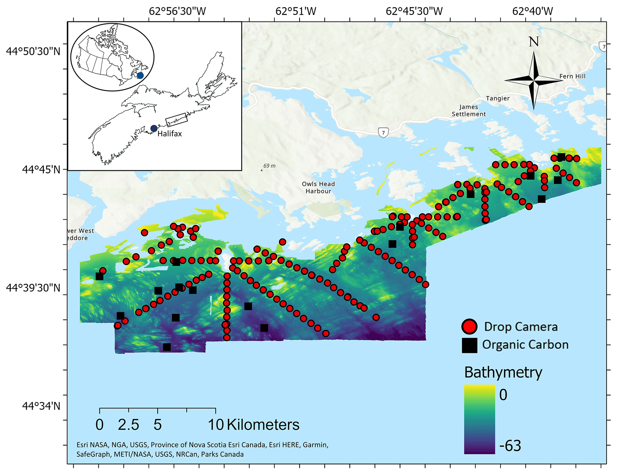
Figure 1 Seafloor MBES bathymetry and sample locations for the survey area at the Eastern Shore Islands, Nova Scotia, Canada (inset).

The study area has a water depth between 31 and 63 m. The surficial geology of the ESI is spatially heterogeneous, with bedrock overlaid by mud, sand, gravel, cobble, and boulder substrates (King, 2018). The bedrock topography is an extension of the terrestrial geomorphology and heavily influences the type and distribution of the surficial deposits. The glacial imprint is substantial in the area, having deposited a sequence of till and glaciomarine mud, which lie directly on the bedrock (King, 2018). There is also a thin layer of wave-modified sand and gravel and of more recent deposits of estuarine mud derived from coastal erosion (Fisheries and Oceans Canada, 2019). Ocean surface temperatures in the ESI are around 1 °C in winter for the 0–100 m depth range and increase in the summer with some stratification leading to surface temperatures exceeding 15 °C (Fisheries and Oceans Canada, 2019). By the fall, mixing deepens this warm layer. Ocean currents run predominantly southwestwards, with some fluctuation around the coast (Feng et al., 2022). The combination of upwelling, currents, and wind allows the mixing of nutrients, acting as an essential component of the marine food web in the region (Fisheries and Oceans Canada, 2019). Nutrients are derived from the river, coastal runoff, and mixing. They are depleted in the spring due to phytoplankton blooms and replenished in the fall when upwelling is predominant (Fisheries and Oceans Canada, 2019). Major human activities in this area include lobster fishing, recreational fishing, and boating, but the human impact is low due to low population density and reduced coastal development compared to Halifax and St. Margarets Bay nearby (Fisheries and Oceans Canada, 2019).

3 Materials and methods

To quantify OC stock in the ESI, sediment samples were collected and OC content and sediment grain size were measured. OC density was calculated for each sample, and four OC stock estimations were generated. The first assumed a homogenous seafloor by scaling up the average OC density to the entire study area. The second also assumed a homogeneous seafloor but used empirical Bayesian kriging (EBK) to derive the spatial variability in OC density for the study area. Both scenarios 1 and 2 were conducted to evaluate OC estimates when no high-resolution mapping data are available. To further refine the OC stock estimates, a substrate classification map was developed by combining high-resolution seafloor predictor variables (derived from multibeam sonar data; see below) and subsea camera imagery of the seabed. The substrate classification map partitioned the study area into hard and soft substrates. The third OC stock estimate utilized the sediment classification and scaled the average OC density to the area of the soft substrate. The final OC stock estimate also utilized the sediment classification map but used empirical Bayesian regression kriging (EBRK) prediction to incorporate the spatial variability in the OC density within the soft substrate only. Scenarios 3 and 4 determine OC estimates when sediment information and high-resolution mapping data are available. An overview of the analysis workflow is shown in Fig. 2.

Figure 2 General analysis steps used to estimate organic carbon in four scenarios.

3.1 Hydrographic datasets

MBES data were collected by the Canadian Hydrographic Service over two separate surveys (20 June–29 July 2019 and 17 August–5 September 2020) (Bondt, 2019, 2020). Three launches were used to complete this survey: the CSL Kestrel, CSL Tern, and CSL Pelican. The survey launch CSL Kestrel was equipped with an R2Sonic 2022 multibeam echosounder. The survey launches CSL Tern and CSL Pelican were outfitted with Kongsberg EM2040C and EM2040C dual head echosounders, respectively. All surveys were conducted at MBES operating frequencies of 200–400 kHz. Vessel position and orientation were corrected in real time by Trimble/Applanix POS MV V5 motion compensation systems. Echosounder data were corrected for sound velocity in real time using Applied Microsystems Limited sound velocity sensors. The vessel position was recorded in real-time using the Can-Net RTK NTRIP connected directly through the POS MV. Raw position and orientation data from the POS MV were logged throughout the survey for further post-processing where required. Bathymetry and backscatter data were processed using the QPS software suite. Bathymetry data were processed in Qimera 2.5.3 to generate a bathymetric digital elevation model (DEM) for the survey area. Backscatter data were processed in FMGT 7.10.2 to generate backscatter mosaics for each of the data sets. Backscatter data were not calibrated; the different survey data sets were harmonized using bulk shift methods (Misiuk et al., 2020, 2021; Haar et al., 2023) from areas of overlap between the survey data sets to generate a corrected backscatter mosaic for the entire study area.

Seafloor morphology features were derived from the primary bathymetric datasets to provide additional predictor variables for sediment classification modeling. These were selected based on literature reviews, expert suggestions, and access to data and were calculated using the Benthic Terrain Modeler (BTM) 3.0 Toolbox in ArcGIS Pro 3.1.2. The terrain features included slope, bathymetric position index (BPI), and vector ruggedness measure (VRM), which are regarded as useful predictors for seabed substrate classification (Stephens and Diesing, 2015; Misiuk et al., 2019) (Table 1) (Fig. 3). The Focal Statistics tool was used to obtain the mean value for each predictor variable over a 20-by-20-pixel neighborhood to reduce noise. The variables were then used in both the substrate map and the OC model.

Table 1 Description of predictor variables used to model sediment type.

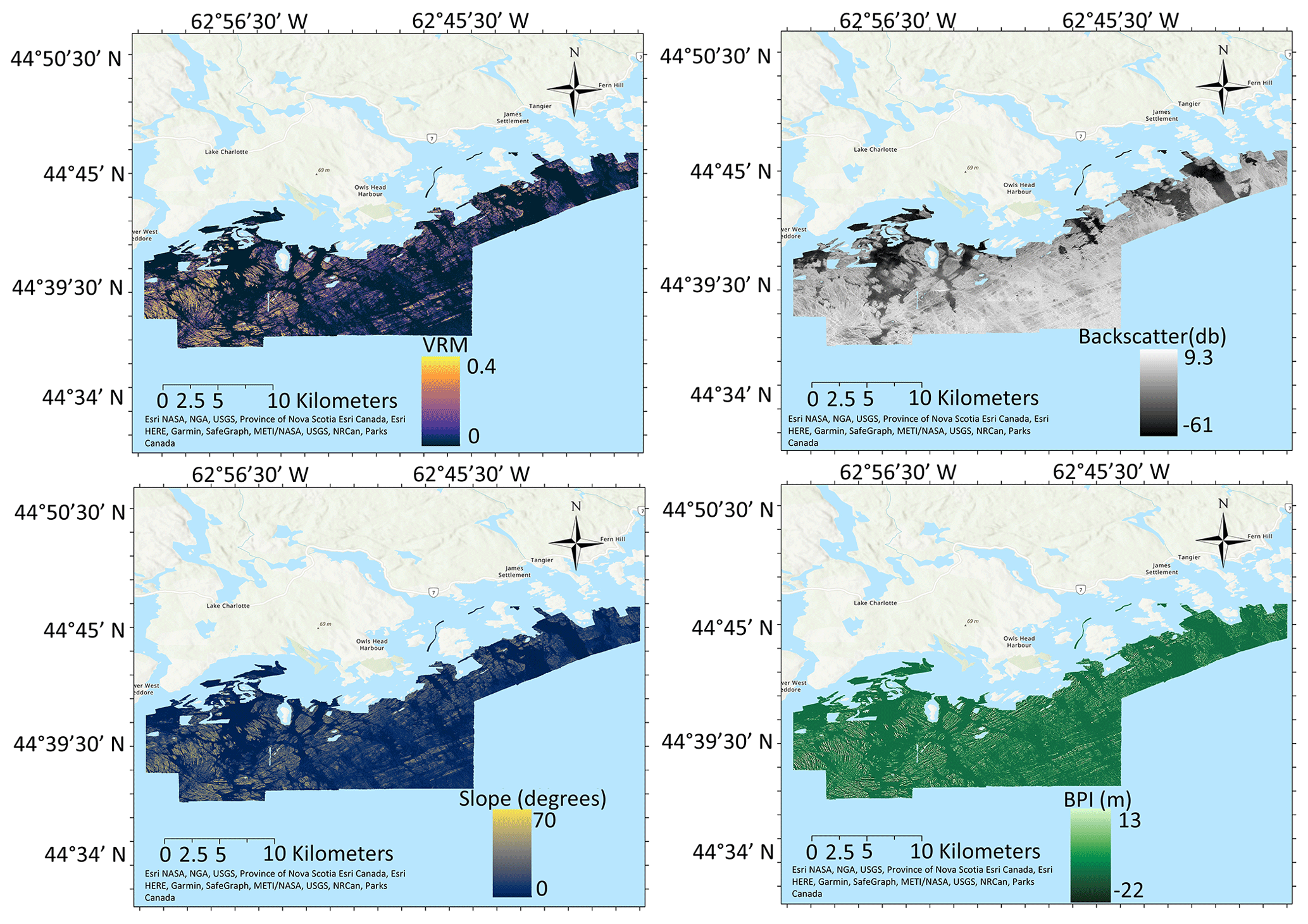
Figure 3 Backscatter, slope, VRM, and BPI data mapped in the Eastern Shore Islands study area.

3.2 Seabed sediment sampling

Sampling surveys for OC and grain size were conducted between 9–27 May 2022 from the MV Island Venture. Sampling locations were randomly placed in regions of low MBES backscatter, which indicate softer, unconsolidated sediments where grab sampling should be successful (Fig. 3). Acoustic backscatter was used as a proxy for sediment grain size to determine areas of soft sediment, and grab sampling locations were randomly selected within this area (Goff et al., 2000; Sutherland et al., 2007; Collier and Brown, 2005; Hunt et al., 2020). A 0.1 m² Van Veen grab fitted with a GoPro camera was operated to collect sediment samples and drop camera imagery at each sample location, with the grab penetrating up to ∼10 cm depth into the substrate. The GPS position of the research vessel was recorded at the point of contact at the seabed at each grab station. A total of 17 grabs were successful in areas of soft substrate. Generally, it is difficult to sample a coarser sediment matrix successfully, and these sediment types are often under-represented in sedimentary carbon studies (Hunt et al., 2020). After thoroughly mixing the sediment in the Van Veen grab, 0.907 kg subsamples of sediment were taken from the grabs and each placed in a plastic container for OC analysis. Following collection, these samples were stored in a cooler during the day and put into a freezer in the evening.

3.3 Processing of sediment grab samples

Prior to sediment grain size and OC analysis, the samples were dried from frozen in the oven at 60 °C overnight and kept in a dark dry cabinet. Sedimentary OC from the grab samples was quantified using an elemental analyzer (EA; Elementar MICRO cube) with a detection limit of 0.03 mg. Based on the method of Verardo et al. (1990), a section of the grab samples (5 g) was ground using a mortar and pestle to form a homogenous powder. Two samples (ES-31 and ES-35) contained significant concentrations of sediment grains coarser than 2 mm (around 30 % of sample). These sand grains were removed using mesh sieves prior to grinding and EA analysis, but final sedimentary OC concentrations were adjusted to total sample weight following EA analysis. Silver capsules were used to weigh the initial mass (0.5–0.7 mg), and acid fumigation was performed by exposing the samples to 37 % hydrochloric acid (HCl) to remove any inorganic carbon. These capsules were then placed in an oven overnight at 60 °C before analysis.

The remaining section of the grab samples was used for sediment grain size analysis, following the protocol of Mason (2011). The sediment was first split into pebble/cobble (>4000 µm), gravel (>2000 µm), and fine-sediment (<2000 µm) material using mesh sieves. The fraction <2000 µm was evaluated using a Beckman Coulter LS 13 320 particle size analyzer at the Bedford Institute of Oceanography. Following the guidance of Mason (2011), the samples were not treated with acid or hydrogen peroxide because the samples had relatively low organic content. The results from the coarse- and fine-scale fractions were combined into a full particle size distribution to determine the percentage of mass of the total for each sample (Supplement). It should be noted that dry bulk density was not measured directly in this study but was instead calculated (see Sect. 3.6).

3.4 Subsea video surveys

A total of 174 drop camera videos were collected by Fisheries and Oceans Canada (DFO) over 13 d during September and October 2017 on board RV Sigma-T (Fisheries and Oceans Canada et al., 2019) (Fig. 1). An HD subsea video camera (SV-HD SDI) was used with camera time and position recorded using a video overlay streamed from the chart plotter (Vandermeulen, 2018). The video feed with overlay outputted to a direct-to-disk HD recorder and a standard low-power LED TV. The GPS antenna for the navigation system was mounted on the roof of the wheelhouse approximately 10 m from the drop camera when deployed off the stern gallows. In this manner, all positional information in the video overlay was offset by ∼10 m and was adjusted during post-processing. Approximately 3 min of moving video was recorded at each drop camera location. The center of each video drift was recorded as the station location. All drop camera sites occurred at depths >10 m. The GoPro camera imagery collected with the grab sampler during OC sampling in 2022 (see section on sediment sampling above) was additionally incorporated with the drop camera imagery for subsequent analysis (Fig. 1).

From each video station, a presence (1) and absence (0) of different sediment types were recorded in post-processing. The data were classified into two sediment types: hard substrate (rock, boulder, cobbles, pebbles, and gravel), and soft substrate (mud and sand) (Fig. 4) (Supplement).

Figure 4 Example of seafloor imagery from each of the two substrate classes: hard substrate (a) and soft substrate (b). Photos from a GoPro camera mounted on the Van Veen grab. Image width is approximately 0.5 m, with the frame of the grab providing scale for classification of substrata.

3.5 Sediment classification model

Random forests has been used in previous carbon mapping studies due to its high predictive accuracy, capacity to manage many predictor variables, and unbiased internal validation (Diesing et al., 2017). In our study, random forests was used to model the sediment grain size class to inform OC content estimation using the randomForest package in R version 4.3.1 (Liaw and Wiener, 2002). The model was initially trained with default hyperparameters (ntree =500, mtry =2, and nodesize =1) using the substrate classification observations and all predictor variables (bathymetry, backscatter, BPI, VRM, and slope). Random forests is an ensemble modeling approach comprising many individual classification trees, each grown on a bootstrapped version of the data set. The observations not selected for a given tree are termed the “out-of-bag” (OOB) observations. Given enough trees, each response observation will be represented in the OOB sample multiple times. By predicting the OOB values for each individual tree during model training, the results can be aggregated over all trees to provide a useful set of validation predictions that were not used to inform training. The OOB observations were used here to estimate predictor variable importance by permuting the predictor values and measuring the resulting increase in OOB error (Liaw and Wiener, 2002). Random forests is generally regarded as robust when using correlated predictors, and estimates of importance additionally suggested contribution to the model by all variables, which were thus retained. Informal trials suggested that a model of 100 trees (i.e., ntree =100) provided sufficient predictive capacity but improved computational speed. After training the final model with these parameters, a confusion matrix was generated using the OOB observations and predictions to evaluate the map accuracy, and the model was then predicted across the full map extent using the predictor variable rasters. The true skill statistic (TSS) was used to evaluate the model predictions, indicating how well predictions agree with observations beyond the level of agreement that could be expected by chance:

$$\begin{array}{}\text{(1)}& \mathrm{TSS}=\mathrm{sensitivity}+\mathrm{specificity}-\mathrm{1},\end{array}$$

where sensitivity is the proportion of observed presences that are predicted as such, and therefore quantifies omission errors, and specificity is the proportion of observed absences that are predicted as such and therefore quantifies commission errors (see Allouche et al., 2006, for an evaluation of this statistic).

3.6 Estimation of standing stock of organic carbon

The elemental analyzer reports OC value as a proportion (weight %). Dry bulk density was not measured directly in this study but was calculated from estimated porosity and grain density. Porosity (ϕ) was calculated from predicted mud content (dimensionless fraction), which is a combination of clay and silt from the grain size distribution measurements using Eq. (2) derived from Jenkins (2005).

$$\begin{array}{}\text{(2)}& \mathit{\varphi }=\mathrm{0.3805}\times C_{\mathrm{mud}}+\mathrm{0.42071},\end{array}$$

where ϕ and C_mud (mud content) are dimensionless fractions. The equation was derived based on data from the Mississippi–Alabama–Florida shelf, and it is assumed that the equation is not site-specific (Diesing et al., 2017).

Dry bulk density (ρ_d) of the sediment was estimated using the porosity and grain density (ϕ_s=2650 kg m⁻³) (Diesing et al., 2017; Hunt et al., 2020):

$$\begin{array}{}\text{(3)}& {\mathit{\rho }}_{\mathrm{d}}=(\mathrm{1}-\mathit{\varphi }){\mathit{\rho }}_{\mathrm{s}}.\end{array}$$

The organic carbon density (kg m⁻³) was calculated by multiplying the %OC (Y) (expressed as a decimal proportion) by the sediment dry bulk density (ρ_d). Following prior studies that quantified marine sedimentary OC (e.g., Diesing et al., 2017; Hunt et al., 2021), the standing stock of organic carbon per grid cell (m_oc) was estimated by multiplying the average OC density by the sampling depth of the Van Veen grab (d=0.1 m) and the area of mapped grid cell (A=4 m²) and was converted to metric tonnes (divided by 1000) using Eq. (4) below:

$$\begin{array}{}\text{(4)}& m_{\mathrm{oc}}=(Y\times {\mathit{\rho }}_{\mathrm{d}}\times d\times A)/\mathrm{1000}.\end{array}$$

Finally, the total standing stock was the m_oc multiplied by the total pixels in the study site (scenarios 1 and 2) or the total pixels in the soft substrate (scenarios 3 and 4).

3.7 Spatial interpolation of organic carbon – no substrate

After the m_oc was calculated for each sample, EBK was used to spatially interpolate m_oc within the entire study site. EBK is a geostatistical interpolation method that builds a kriging model by subsetting the study area, coupled with multiple simulations to obtain the best fit (Krivoruchko and Gribov, 2019). This process finally creates several simulated semi-variograms, each of which is an estimate of the true semi-variogram for the subset (Pellicone et al., 2018). EBK differs from other kriging methods, since it considers the uncertainty in the semi-variogram estimation step, providing an estimate of the prediction standard errors. An exponential semi-variogram and an empirical transformation were selected, and EBK was executed in the geostatistical wizard in Esri ArcGIS Pro 3.1.

3.8 Spatial interpolation of organic carbon density – soft substrate

EBRK was used for the spatial interpolation of OC density and estimation of values at unknown locations within the extent of the soft substrate. EBRK is a geostatistical interpolation method that combines ordinary least-squares regression and kriging to provide accurate predictions of non-stationary data at a local scale (Giustini et al., 2019). An exponential semi-variogram model and an empirical transformation were selected for the EBRK model, which was evaluated using leave-one-out cross-validation (Mallik et al., 2022). The EBRK method is different to EBK in that predictor variable information is accommodated by including the principal components as regression variables prior to the kriging step. Thus, all the predictor variables from the substrate classification map (bathymetry, backscatter, BPI, VRM, and slope) were masked to the soft-substrate area in Esri ArcGIS Pro 3.1 and included in the EBRK model to improve estimation of OC density.

3.9 Cross-validation methods

To estimate the accuracy of the EBK and EBRK predictions, the mean error (ME) and the root-mean-square error (RMSE) were calculated. The ME is the average of the cross-validation errors, measures model bias, and should have a value close to zero (Acharya and Panigrahi, 2016).

$$\begin{array}{}\text{(5)}& \mathrm{ME}={\displaystyle \frac{\mathrm{1}}{n}}{\sum }_{i=\mathrm{1}}^n\mathit{\{}z\left(xi\right)-\widehat{z}\left(xi\right)\mathit{\}}\end{array}$$

The RMSE measures the difference between the predicted and the observed values and estimates the standard deviation of the residuals (Boumpoulis et al., 2023). A small RMSE indicates that the model has performed well and can predict the data accurately.

$$\begin{array}{}\text{(6)}& \mathrm{RMSE}={\left[{\displaystyle \frac{\mathrm{1}}{n}}{\sum }_{i=\mathrm{1}}^n\mathit{\left\{}z\right(xi)-\widehat{z}(xi){\mathit{\}}}^{\mathrm{2}}\right]}^{\mathrm{1}/\mathrm{2}}\end{array}$$

z(xi) is the observed OC, $\widehat{z}$ (xi) is the prediction of OC at location xi, and n is the number of observations. These cross-validation error parameters were calculated within the Geostatistical Wizard Tool in Esri ArcGIS Pro 3.1.

4 Results

4.1 Grain size distributions, sediment properties, and organic carbon content

Van Veen grab samples provided grain size and OC measurements at each station (Table 2). It is important to note that silt and clay were merged into a single mud class to estimate the OC stock (Burdige, 2007; Hedges and Keil, 1995).

Table 2 Raw data from grab samples, including grain size and OC measurements.

4.2 Relationship between grain size and organic carbon

A linear regression was performed to examine the relationship between OC content (%) and the percentage grain size composition of mud. There was a significant positive relationship between OC content and percent mud (p<0.001; R²=0.81) (Fig. 5), suggesting that percent mud content may be useful as a proxy for OC content, as also observed at many other sites (Burdige, 2007; Hedges and Keil, 1995; Hunt et al., 2021).

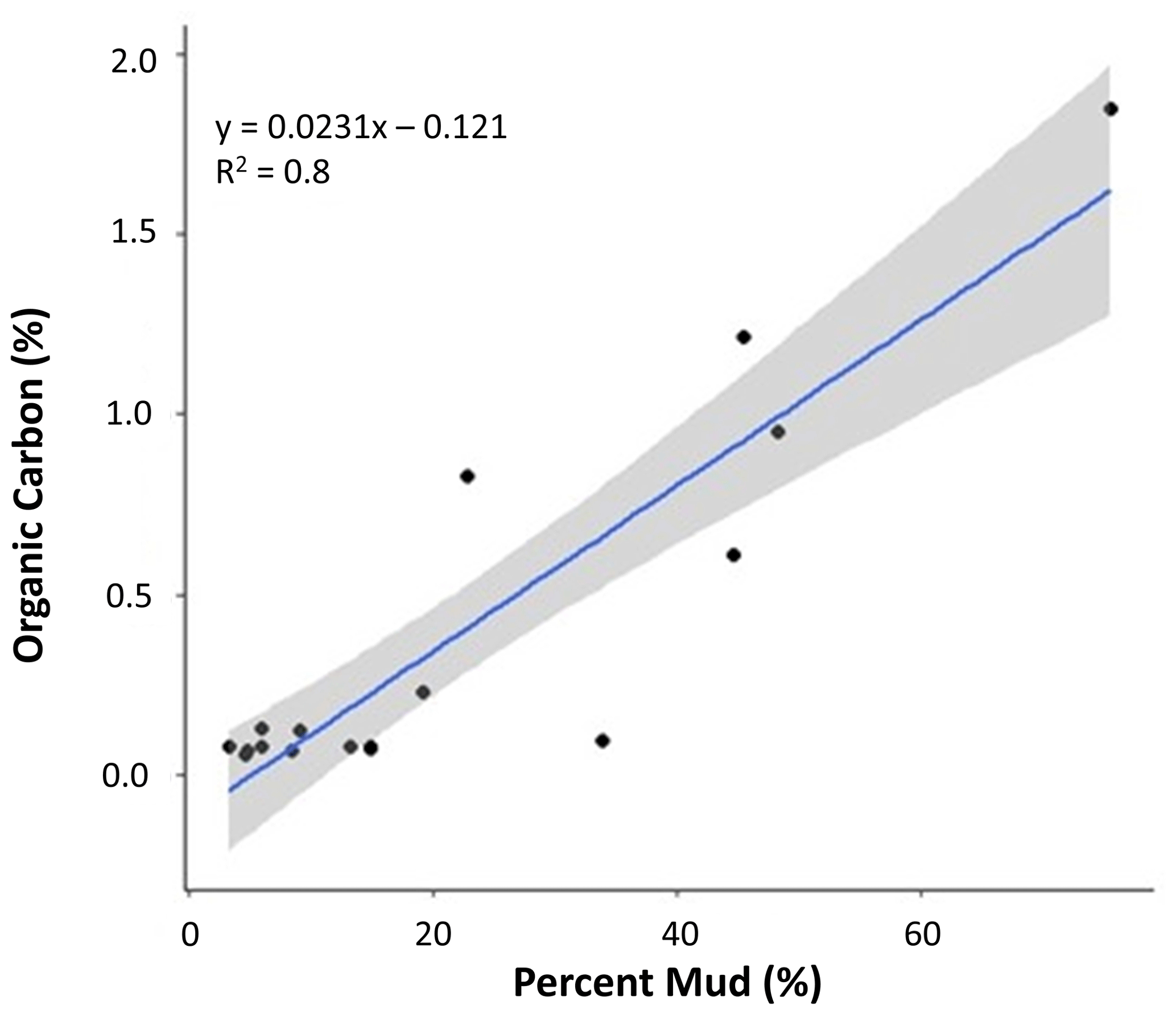
Figure 5 Linear regression indicating the relationship between OC and percent mud. The gray area represents a 95 % confidence interval for the slope of the regression line.

4.3 Substrate classification map

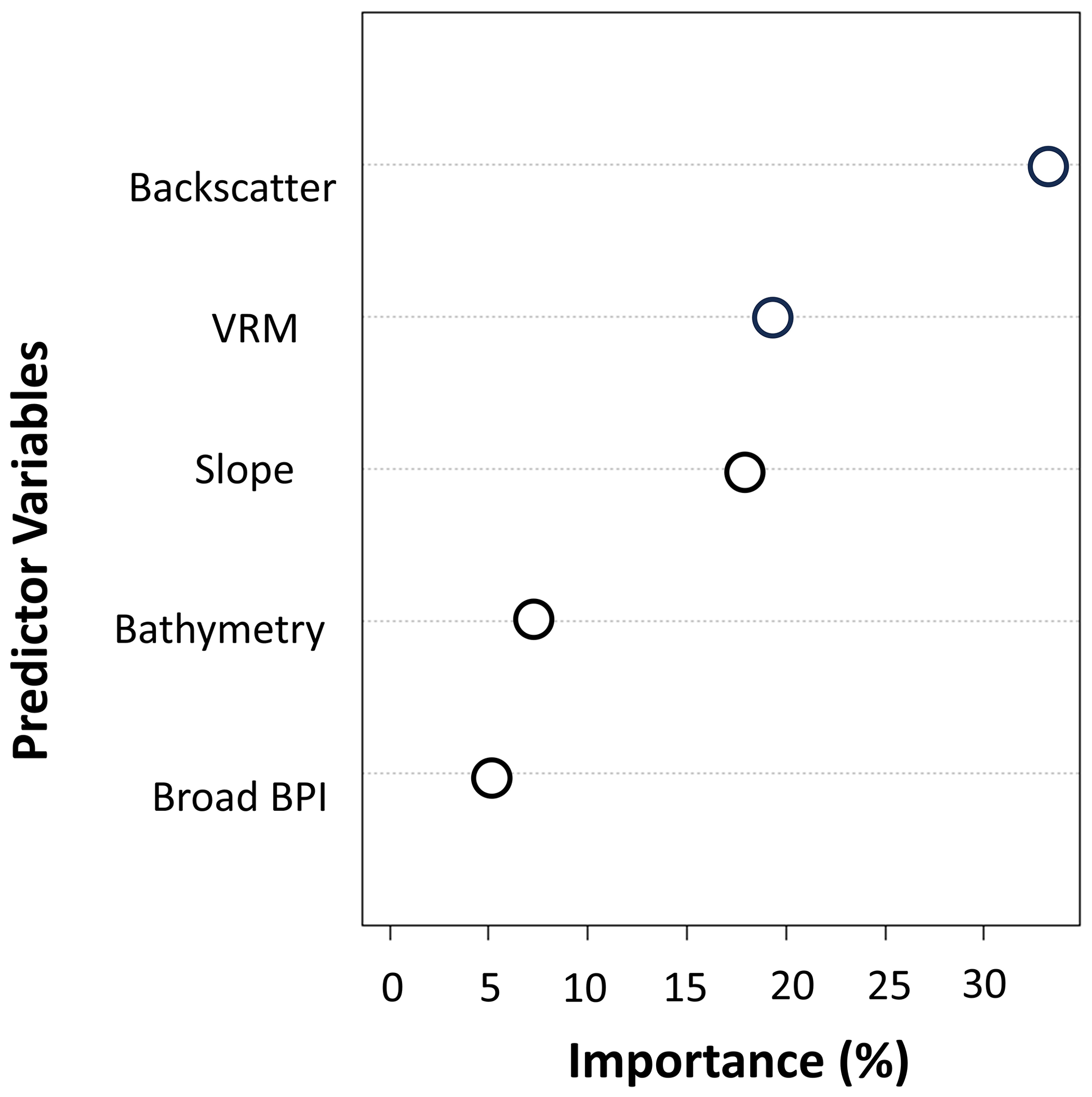
Outputs from random forests indicated that bathymetry, backscatter, vector ruggedness measure (VRM), and slope were all important for the sediment classification. Figure 6 shows the relative importance of the five variables in the model. Backscatter was the most important variable for predicting sediment type, followed by VRM, slope, bathymetry, and BPI.

Figure 6 The importance of predictor variables as estimated using random forests.

The confusion matrix calculated using the OOB observations is presented in Table 3. A TSS score of 0.67 indicates substantial agreement between observations and predictions of each class, suggesting that the model was able to successfully differentiate soft and hard substrates within the study area.

Table 3 Confusion matrix of substrate type predictions.

The sediment classification map revealed that the hard substrate was the most spatially extensive (178 km²), whereas the soft-substrate class was smaller, covering approximately 45 km² of the study area, corresponding with contiguous patches of relatively low-relief seafloor (Fig. 8). Sediment grain size from the grab samples from the soft-sediment areas revealed grain size percentiles d₁₀=17, d₅₀=147, and d₉₀=1822 µm. This suggests predominantly sandy sediments, with varying smaller proportions of silt and clay (Fig. 7). Two samples comprised around 30 % coarse substrate (>2000 µm) (Fig. 7).

Figure 7 Sediment classification map indicating predicted soft (orange) and hard (blue) substrates. Pie charts depict ratios of sand (yellow), silt (orange red), clay (purple), and coarse (green) for each sediment sample collected.

Figure 8 Sediment classification map indicating areas of soft (orange) and hard (blue) substrate. Proportional symbols of OC indicate the sampled percentage (yellow).

4.4 Organic carbon density maps

Cross-validation of the EBK model indicated the accuracy of the OC density predictions was ME $=-\mathrm{0.27}$ and RMSE =4.21 kg m⁻³, suggesting low bias but also that the magnitude of prediction error was substantial compared to the range of the observed data (e.g., Fig. 9). Predicted OC density was high on the western part of the study site near Lower West Jeddore and in the middle of the study area near Owls Head Harbour (Fig. 9).

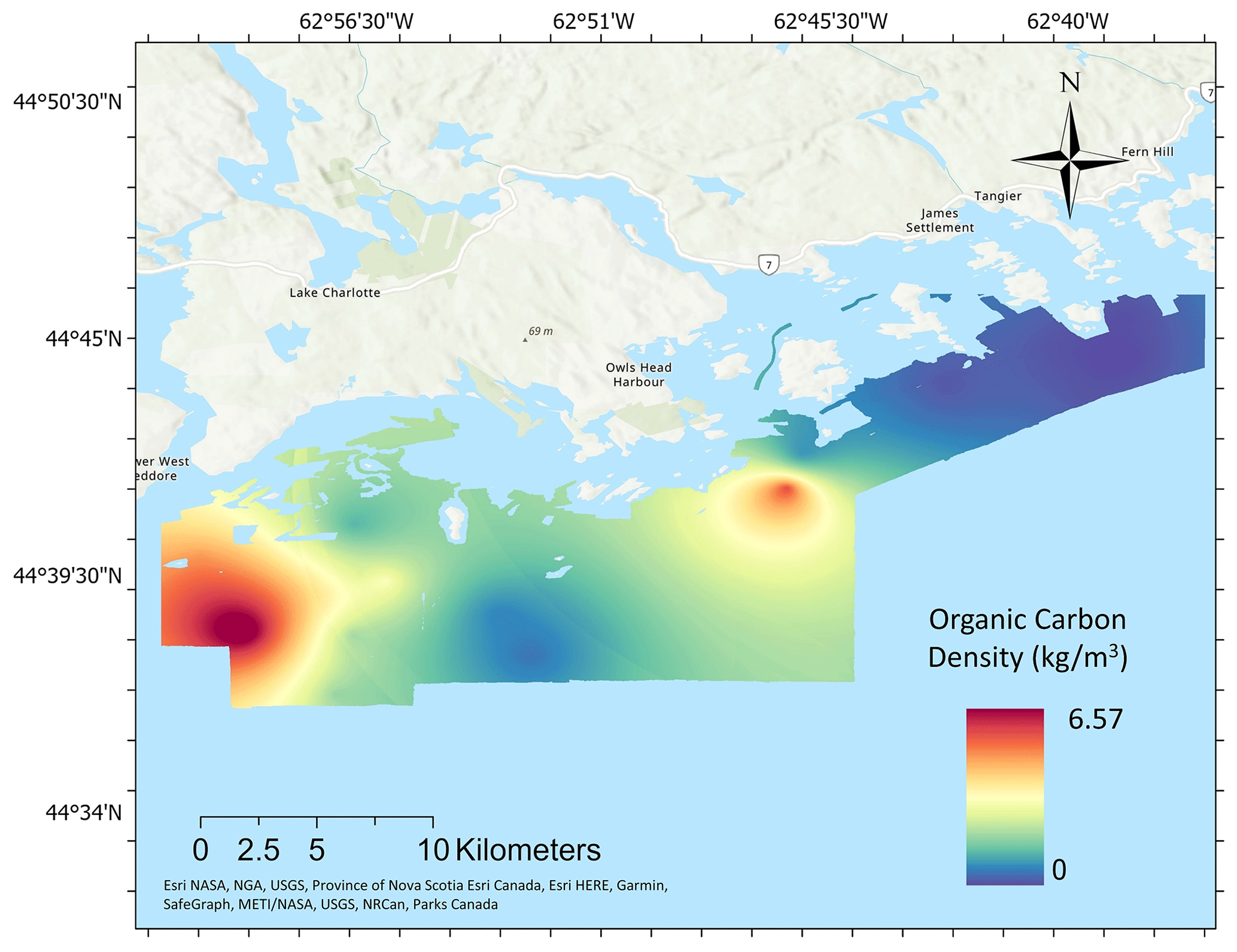
Figure 9 Spatial interpolation of OC using EBK.

Cross-validation of the EBRK model indicated ME $=-\mathrm{0.31}$ and RMSE =3.52 kg m⁻³, suggesting slightly higher bias than the EBK model yet more accurate predictions. The EBRK model prediction suggested high OC density in the west and southwest of the study area. A significant quantity of OC density was predicted eastward near Owls Head Harbour (Fig. 10). The lowest OC density was predicted in the eastern part of the study area with quantities close to zero.

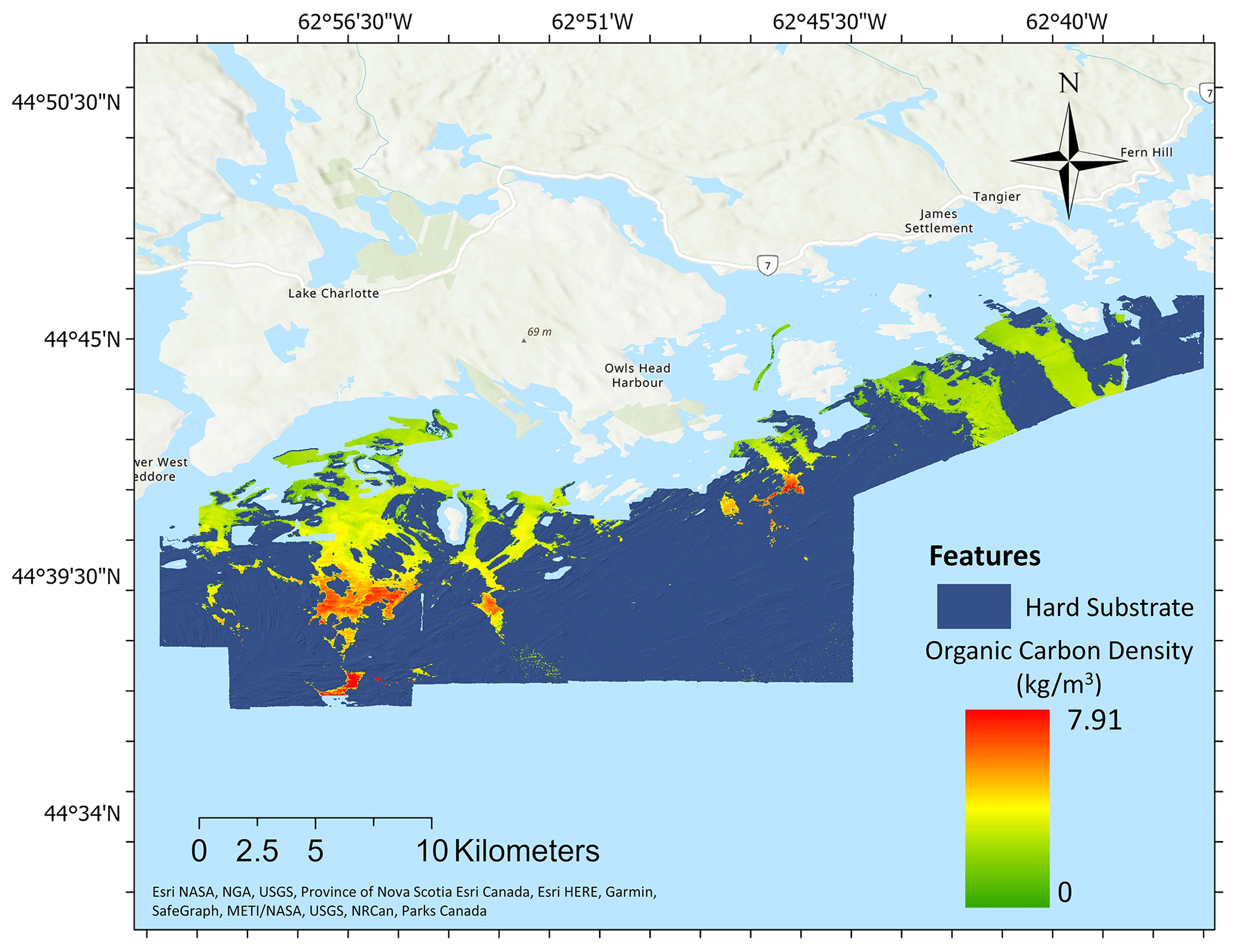
Figure 10 Spatial interpolation of OC using EBRK.

4.5 Organic carbon estimates

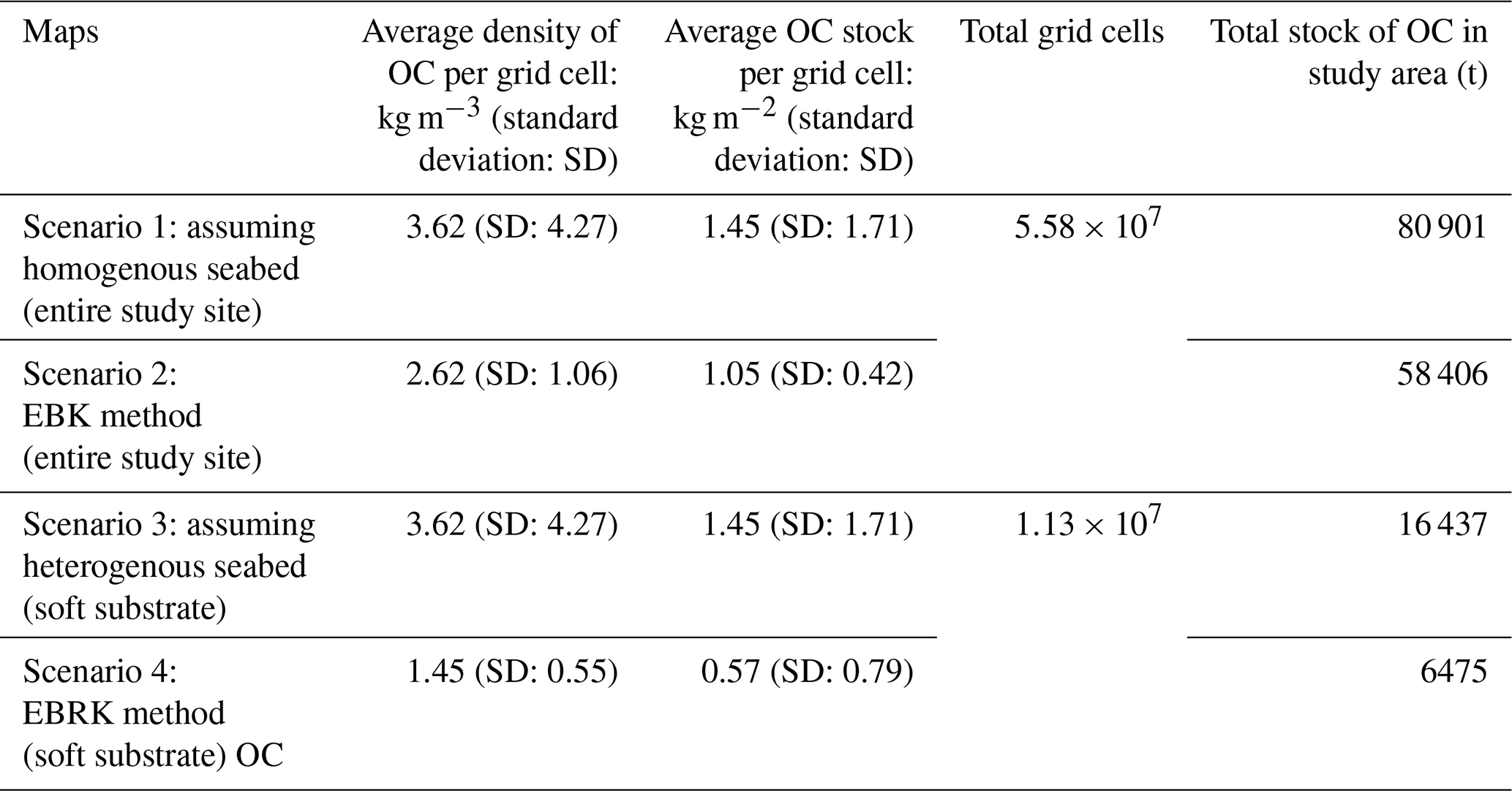
Estimates of average OC density, OC stock per pixel, and total OC stock were calculated for all four scenarios (Table 4). For scenario 1, the average OC stock per grid cell was used to scale up to the full spatial extent of the study site. For scenario 3, the average OC stock per grid cell was used to scale up to the full spatial extent of only the soft-sediment area. For scenarios 2 and 4, total standing stocks were calculated by summing the predicted pixel values for either the full study extent (scenario 2) or the soft-sediment area (scenario 4).

Table 4 Calculations used to determine the total stock of OC in the mud/sand sediment type and the total stock of OC in the entire study area.

5 Discussion

Our study explores how high-resolution spatial models can improve carbon budget estimates. We have described a quantitative spatial model of hard and soft substrate in a continental shelf environment and determined four estimates of OC stock in the surficial sediments (top 10 cm): scaling to the entire study area (scenario 1), interpolating OC density using an EBK model (scenario 2), scaling to only the soft substrate (scenario 3), and refining m_oc within the soft substrate estimated from an EBRK model (scenario 4). The results demonstrate that, as spatial models become more detailed, the OC stock estimation increases in accuracy but decreases the overall predicted OC stock.

5.1 Evaluation of sediment map

The sediment map effectively classified the hard and soft substrate (TSS =0.67) and significantly refined our understanding of the detailed distribution of the OC. Previous studies applied similar machine learning modeling approaches with success (Stephens and Diesing et al., 2015; Misiuk et al., 2019; Mitchell et al., 2019; Epstein et al., 2024). Our results further demonstrate that this approach is suitable for mapping benthic substrates where high-resolution MBES data sets and suitable sediment ground truthing are available. Other studies found that the highest POC concentrations are associated with gravelly mud, mud, and sandy mud (Diesing et al., 2017). This agrees with our linear regression that areas of increased OC have a high mud content (Fig. 5). The empirical relationship observed between mud content and OC strongly suggests the importance of using substrate maps to precisely estimate the stock of OC.

5.2 Variability in organic carbon stocks

Differences in estimated OC stock suggest that the substrate map was an essential component to this study. Smeaton et al. (2021) note that the seafloor is commonly assumed homogenous in benthic OC studies. Shelf environments are inherently heterogeneous, and scaling up OC measurements where high-resolution mapping data are available offers an effective way of obtaining accurate estimates of OC in these areas (Snelgrove et al., 2018). To improve estimates and better identify how the ocean carbon cycle will be altered by climate change and possibly human activities, carbon studies should embrace the full complexity of the seafloor (Snelgrove et al., 2018; Epstein et al., 2024). Our study emphasizes the benefits of high-resolution MBES data for such applications and the need for additional coverage and collection of seafloor mapping data sets in coastal waters where coverage is currently limited (Mayer et al., 2018).

The difference in the total m_OC calculated based on the substrate map (16 437 and 6475 t of OC) versus estimates in the absence of a map (80 901 and 58 406 t of OC) emphasizes that a spatial component to OC estimations is essential for carbon system models. This difference demonstrates the need to understand the presence of hard substrate at the seabed when calculating carbon stocks as suggested in recent broad-scale carbon modeling studies (Epstein et al., 2024). Currently, global carbon models oversimplify carbon processes due to a lack of information and data on the complexity of the marine carbon cycle. For instance, previous studies examined carbon quantity at the surface of the ocean by analyzing phytoplankton activity using satellite imagery, since there is an assumption that carbon at the surface of the ocean correlates with areas of high carbon storage at the seafloor (Chase et al., 2022). This assumption ignores the complexity of carbon moving through the pelagic and benthic regions. Spatially continuous seafloor mapping data are a step towards improving accuracy in our estimation, which will enhance the ongoing investigations into the marine carbon cycle.

Additionally, the resolution of the seafloor mapping data is important when modeling OC. For instance, by using a 2 m by 2 m grid resolution, we can interpolate the carbon within the soft substrate using EBRK models. Through the EBRK interpolation of carbon, the carbon stock (6475 Mt of OC) was less than the estimates that assume a homogenous soft substrate. The EBRK method indicates that high-resolution interpolated models of OC can help to further refine standing stock estimates and provide insight into where the carbon hotspots are within the study area.

The estimates from our study were compared to the paper by Epstein et al. (2024), since they evaluated organic carbon stock in the entire Canadian continental margin, which included our study area. To compare these estimates, we clipped their OC density map to our study site and found that the mean OC density was 7.12 kg m⁻³ (SD: 1.93). This mean OC density is higher than but falls within the standard deviation of values for scenarios 1 and 3 presented here (Table 4). To compare the total OC stock for the study region, we adjusted the depth used by Epstein et al. (2024) from 0.3 to 0.1 m by dividing their OC stock estimates by 3. The OC stock was 161 552 t (SD: 43 723), which is higher than any of the estimates under the four scenarios we present (Table 4). One reason for the higher estimates in the study by Epstein et al. (2024) could be that no OC measurements within the study region were available in Epstein et al. (2024). Therefore, their model relied on OC data outside this area, which could lead to error. Furthermore, an underrepresentation of zero values in the response data could lead to an overestimation of organic carbon standing stocks in their study, as zero values are unlikely to be predicted from model outputs. The comparison between both studies highlights the importance of high-resolution sediment classification maps when estimating sedimentary OC stock; knowing the extent of bedrock can reduce the overestimation of OC content substantially.

5.3 Organic carbon maps

When comparing the EBK and EBRK carbon maps, there were some similarities and differences. Both maps indicate a hotspot near Owls Head Harbour and low OC density on the eastern side of the study area. However, the EBK map shows a large area of high OC density on the western side of the study area, whereas the EBRK model has a smaller area slightly east of that location. These differences between the models emphasize that the EBK model could have some inaccurate interpolation due to the limited sediment samples in the study area. In contrast, the EBRK model was performed in the soft substrate, where all the samples were distributed, with fewer data gaps. The EBK model indicates that, without high-resolution seafloor mapping data, one can obtain a general understanding of OC hotspots. However, the EBRK model can provide a more precise understanding of the spatial variability in OC density in the study site.

Both maps suggest high OC densities associated with locations further offshore (Figs. 9 and 10) and within sediments containing increased amounts of silt and sand (Figs. 7 and 8). Based on previous evaluations of the study area, inshore sediment often comprised bedrock with patchy sand and gravel, whereas, further offshore, there is thick glacial marine mud over bedrock (Fisheries and Oceans Canada, 2019). This geomorphology could be the cause of higher OC density further offshore. The cause of increased OC content near Owls Head Harbour remains uncertain, lacking any aquaculture or substantial runoff from nearby agriculture. However, the ESI has substantial kelp and eelgrass beds; future research may explore relationships between these environments and OC.

5.4 Limitations of the study

The lack of dry bulk density measurements for the OC stock calculations was a major limitation of this study. The use of a dry bulk density equation derived from a previous study could introduce error into calculations based on regional geological differences. Only two seabed sediment classes were mapped here, which does not represent the actual complexity of substrate types within the ESI. Preliminary random forest model runs that incorporated additional sediment classes showed high error and poor performance, likely due to the difficulty in accurately determining sediment types from a small number of subsea video samples. We emphasize challenges associated with differentiating complex substrate classes that were noted in previous similar studies (e.g., Diesing et al., 2020).

We have also assumed here that there is no OC in the hard substrate. The hard-substrate class included more than bedrock, with regions of mixed sediment, such as gravelly mud, visible in the subsea video which could contain some OC. Thus, improving the sediment classification map to include more complex substrates could improve the OC stock estimates further. The limited number of OC samples may have skewed the interpolation, since the data points were not uniformly distributed within the areas of soft substrate. We therefore recommend higher sampling densities for future OC studies.

These limitations highlight the challenges of carbon modeling on the seafloor and the need for further research into evaluating the correct procedure for utilizing sediment classification maps when predicting OC stock. Furthermore, there is persistent uncertainty surrounding how much sea surface particulate OC (POC) reaches the seafloor and the spatial distribution of the sinks of this material. Thus, future carbon studies should evaluate benthic–pelagic coupling and the impact it has on OC stocks.

5.5 Future implications of organic carbon models

Marine spatial planners are trying to manage the seabed in a sustainable manner, and high-resolution regional-scale OC mapping data could be a practical option to help identify vulnerable C stores and hotspots and to determine how these areas may be altered due to environmental change and anthropogenic activities (Hunt et al., 2021). MPAs have been defined as regions that conserve marine resources, ecosystem services, or cultural heritage (Laffoley et al., 2019). High-resolution seafloor OC models could help redefine MPAs and allow them to incorporate areas of high carbon stock. It is important to recognize sediments as long-term carbon sinks that provide climate regulation services.

It is challenging to measure how human activities like bottom trawling are impacting the seabed and how they influence OC without an understanding of the natural processes of marine carbon cycling. Studies that examine OC spatially and examine its connections to seafloor composition are a crucial component to piecing together the natural marine carbon cycle, which can help determine if the amount of remineralization occurring from human activities will have a substantial impact on climate. Even with a relatively limited number of OC samples, this study demonstrates that high-resolution seafloor substrate maps and spatial OC models are critical to understanding the spatial heterogeneity of OC on the seafloor.

6 Conclusions

In this study, we generated a high-resolution sediment map that accurately captured the spatial complexity and distribution of broad sediment types in the ESI area. Through the four scenarios for estimating OC stocks, we demonstrated that seafloor sediments are a good high-resolution proxy that enable accurate estimation of OC stock in the area and that information (or lack of information) regarding the spatial heterogeneity of the seafloor substrata substantially influences estimates of OC stock (ranging from 6475–80 901 t of OC). These results emphasize that further research should explore high-resolution multibeam echosounder data in determining OC-rich hotspots to improve our understanding of the role that benthic systems play as global carbon stores and of how the management of these systems can contribute towards climate change management strategies and marine climate policy.