Effect of terrestrial nutrient limitation on the estimation of the remaining carbon budget

The carbon cycle plays a foundational role in the estimation of the remaining carbon budget. It is intrinsic for the determination of the transient climate response to cumulative CO₂ emissions and the zero-emissions commitment. For the terrestrial carbon cycle, nutrient limitation is a core regulation on the amount of carbon fixed by terrestrial vegetation. Hence, the addition of nutrients such as nitrogen and phosphorus in land model structures in Earth system models is essential for an accurate representation of the carbon cycle feedback in future climate projections. Therefore, the estimation of the remaining carbon budget is impacted by the representation of nutrient limitation in modelled terrestrial ecosystems; however, it is rarely accounted for. Here, we estimate the carbon budget and remaining carbon budget of a nutrient-limited Earth system model, using nitrogen and phosphorus cycles to limit vegetation productivity and biomass. We use eight Shared Socioeconomic Pathways (hereafter SSP) scenarios and idealized experiments with three distinct model structures: (1) carbon cycle without nutrient limitation, (2) carbon cycle with terrestrial nitrogen limitation, and (3) carbon cycle with terrestrial nitrogen and phosphorus limitation. To capture the uncertainty in the remaining carbon budget, three different climate sensitives were tuned for each model version. Our results show that, overall, nutrient limitation reduced the remaining carbon budget for all simulations in comparison with the carbon cycle without nutrient limitation. Between nitrogen and nitrogen–phosphorus limitation, the latter had the lowest remaining carbon budget. The mean remaining carbon budgets obtained from the SSP scenario simulations for the 1.5 °C target in the non-nutrient-limited, nitrogen-limited, and nitrogen–phosphorus-limited models were 228, 185, and 175 Pg C, respectively, relative to the year 2020. For the 2 °C target, the mean remaining carbon budget values were 471, 373, and 351 Pg C for the non-nutrient-limited, nitrogen-limited, and nitrogen–phosphorus-limited models, respectively, relative to the year 2020. This represents a reduction of 19 % and 24 % for the 1.5 °C target and 21 % and 26 % for the 2 °C target for the respective nitrogen- and nitrogen–phosphorus-limited simulations compared with the non-nutrient-limited model. These results show that terrestrial nutrient limitation constitutes an important factor to be considered when estimating or interpreting remaining carbon budgets and that it is an essential uncertainty in the remaining carbon budgets from Earth system model simulations.

1 Introduction

Future climate projections have only rarely accounted for nutrient limitation of the land carbon sink (Wang and Goll, 2021). This weakness was partially overcome in Phase 6 of the Coupled Model Intercomparison Project (CMIP6), with more Earth system models (ESMs) embracing nitrogen (N) limitation as a standard for terrestrial system structures. However, the inclusion of phosphorus (P) remains rare, and the representation of micronutrients remains a distant ambition (Arora et al., 2020; Spafford and MacDougall, 2021). Thus, the future of the land carbon sink remains uncertain, as projecting the interactions between the terrestrial system and atmosphere is a challenge without fully accounting for nutrient limitations (Achad et al., 2016). Since the year 1850, the cumulative CO₂ land sink has been estimated to be 210 ± 45 Pg C, which represents 31 % of all anthropogenic carbon emissions (Friedlingstein et al., 2022). The terrestrial carbon sink has increased historically with an increasing CO₂ emission rate such that the proportion of carbon taken up by land has remained close to constant (Friedlingstein et al., 2022).

Nutrient availability constrains the capacity and rate at which terrestrial plants assimilate carbon (Goll et al., 2012). N and P are the nutrients that most commonly limit vegetation growth (Filipelli, 2002; Fowler et al., 2013; Wang et al., 2010; Du et al., 2020); hence, they have been the subject of most research and large-scale modelling efforts. Globally, this effect varies. Most of the terrestrial biosphere is co-limited by both N and P, with N being the dominant limiting nutrient at higher latitudes, whereas P dominates at lower latitudes (Du et al., 2020). Earth system models are designed to account for land use change and biological productivity when estimating the carbon sink on land (Kiwamiya, 2020). The change in the nutrient concentration in terrestrial systems in future simulations is an uncertainty with respect to determining the land carbon sink over the next decades (Shibata et al., 2010, 2015; Menge et al., 2012). Complicating this problem further, a large portion of nutrients on land are derived from anthropogenic sources, including agricultural fertilization (artificial, compost and manure), atmospheric deposition of N-bearing pollutants, and urban wastewater discharge (Lu and Tian, 2017; van Puijenbroek et al., 2019).

It is likely that the first generation of ESM simulations overestimated how much terrestrial ecosystems would respond to an increase in the atmospheric carbon dioxide concentration based on carbon-only schemes (Wieder et al., 2015). A large amount of terrestrial carbon uptake was predicted by those simulations, which would result in unrealistic nutrient requirements. For example, in a study by Wieder et al. (2015), ESMs with N and N–P limitation were projected to decrease net primary productivity by 19 % and 25 %, respectively. Hence, the implementation of nutrient limitation in ESMs has been shown to improve the representation of carbon uptake on land (Wang et al., 2007, 2010; Goll et al., 2017; De Sisto et al., 2023) and, thus, will affect the carbon budget.

The carbon budgets can be seen from two perspectives. The first describes pools and fluxes of carbon within the Earth system (Friedlingstein et al., 2022). This perspective serves to understand how natural sinks respond to changes in climate, CO₂, and CH₄. The second describes the remaining carbon budget: the allowable future CO₂ emissions to reach a temperature target, commonly 1.5 and 2 °C. The remaining carbon budget is derived from another metric, the transient climate response to cumulative CO₂ emission (TCRE), which quantifies how global surface temperatures are nearly proportional to cumulative CO₂ emissions (Matthews et al., 2009; MacDougall, 2016; Spafford and MacDougall, 2020). As the TCRE represents the proportionality of cumulative CO₂ emission to its accompanying temperature change, its inverse can be used to estimate the remaining carbon budget for temperature targets (Matthews et al., 2020). The TCRE has been shown to be a good metric for predicting the response of temperature to cumulative CO₂ emissions. However, this metric only represents warming from CO₂ emissions, excluding the impacts of non-CO₂ forcing agents. A method to account for this issue is to use simulations including all anthropogenic forcing and to plot the total anthropogenic warming as a function of cumulative CO₂ emissions, also known as the “effective TCRE” (Tokarska et al., 2018). There is a large uncertainty in TCRE estimates, with a likely range from 1.0 to 2.3 K EgC⁻¹ (IPCC, 2021). For idealized experiments the transient climate response (TCR) can be used to quantify the physical uncertainty in the TCRE. The TCR is the amount of global warming expected to occur when atmospheric CO₂ concentrations double from their pre-industrial levels, while all other factors remain constant. This corresponds to year 70 in a 1pctCO2 experiment, in which the annual CO₂ concentration is increased at a rate of 1 % yr⁻¹ (Eyring et al., 2016). The TCR is dependent on the CO₂ concentration rates represented in the input datasets. Hence, unlike the TCRE, the TCR is dependent on the scenario used to compute it (e.g. MacDougall, 2017). The other important source of variability among TCRE estimates comes from uncertainties in carbon uptake by the ocean and terrestrial biosphere.

Terrestrial system nutrient limitation plays a vital role in the estimation of the remaining carbon budget due to its effect on the carbon cycle. Accounting for P limitation in carbon budget estimations is desirable due to its limiting effect at low latitudes (Du et al., 2020). Hence, the impacts of P on terrestrial vegetation biomass and the limitation of the carbon sink almost certainly affect remaining carbon budget estimates. This study assesses how nutrient limitation affects several uncertainties in remaining carbon budget estimates, including uncertainty in the TCRE, the estimated contribution of non-CO₂ climate forcings to future warming, the correction for the feedback processes presently unrepresented by Earth system models, and the unrealized warming from past CO₂ emissions – called the zero-emissions commitment (ZEC) (Rojelj et al., 2018). In addition to these four factors, knowledge of the human-induced warming to date is needed to compute the remaining carbon budget. This value is well estimated from historical records (Arias et al., 2021). Nutrient limitation can be used to improve historical warming accuracy in emission-forced ESM simulations (De Sisto et al., 2023). The TCRE represents the response of temperatures to CO₂ emissions; hence, different models can represent different remaining carbon budgets based on different carbon–climate sensitivities. The non-CO₂ emissions affect the change in temperatures and need to be understood to maintain desired temperature targets. Moreover, the change in temperature after emission cessation is an important dynamic that should be understood and considered in remaining carbon budget estimations. In future projections, non-CO₂ climate forcings are likely affected by the introduction of nutrient limitation in ESMs. The main impacts include feedback changes due to the land carbon sink and land use change emission variation (including albedo changes), either by photosynthetic limitation or a reduction in terrestrial vegetation biomass. These changes might also impact the expected warming contribution after CO₂ emissions are ceased. Lastly, within this remaining carbon budget framework, N and P constitute an unrepresented source of Earth system feedback that is now accounted for in the present simulations.

Isolating the effects of N and P terrestrial limitation provides a novel insight into how underrepresented process in terrestrial systems contribute to remaining carbon budget uncertainties. Therefore, it is important to understand how ESM carbon cycle sensitivity to nutrient limitation constrains the land carbon sink in future simulations. Hence, we explore the effect of terrestrial N and P limitation in remaining carbon budget estimates using an intermediate-complexity Earth system model and employing historical, idealized, and Shared Socioeconomic Pathways (hereafter SSP) projections.

2 Methodology

2.1 Model description

Simulations to quantify the remaining carbon budgets were carried out with the University of Victoria Earth System Climate Model (UVic ESCM). The UVic ESCM (version 2.10) is a global, intermediate-complexity model (Weaver et al., 2001; Mengis et al., 2020). The model is comprised of a 3D dynamic ocean circulation model (Pacanowski, 1995), a simplified moisture–energy balance atmosphere (Fanning and Weaver, 1996), a dynamic–thermodynamic sea ice model (Bitz et al., 2001), and a land surface model (Meissner et al., 2003).

In the model, the terrestrial and oceanic carbon cycles are represented. The ocean comprises 19 vertical levels that become thicker with depth (50 m near the surface to 500 m in the deep ocean). Ocean biogeochemistry is based on a simple nutrient–phytoplankton–zooplankton–detritus model (Keller et al., 2012; Schmittner et al., 2005), with representation of the ocean carbonate chemistry and sediments (Mengis et al., 2020).

In version 2.10 of the model, the soil is represented by 14 subsurface layers. The thickness of these layers increases exponentially with depth, with the surface layer measuring 0.1 m, the bottom layer measuring 104.4 m, and the total layer measuring 250 m. Hydrological processes are active in the first eight soil layers (top 10 m), whereas the layers below have granitic characteristics. The soil carbon cycle is active up to a depth of 3.35 m (six layers) (Avis, 2012; MacDougall et al., 2012). TRIFFID (Top-down Representation of Interactive Foliage and Flora Including Dynamics) represents vegetation interaction between five plant functional types within the terrestrial vegetation. Based on the Lotka–Volterra equations (Cox, 2001), broadleaf trees, needleleaf trees, shrubs, C₃ grasses, and C₄ grasses compete for space in the grid. Appendix Fig. C1 shows the representation of above-ground vegetation biomass using the UVic ESCM compared to the Santoro et al. (2024) dataset. Carbon is taken up and allocated to growth and respiration via photosynthesis. The carbon from vegetation is then transferred to the soil through litter fall and allocated to the soil as a decreasing function of depth. Permafrost carbon is prognostically generated within the model using a diffusion-based scheme meant to approximate the process of cryoturbation (MacDougall and Knutti, 2016).

The UVic ESCM prescribes anthropogenic land use changes based on the standardized CMIP6 land use forcing (Ma et al., 2020) regridded to the UVic ESCM grids. Land use data products have been modified for use by the UVic ESCM by aggregating cropland and grazing land into one crop type, representing any of the five functional types of crops, and one grazing variable, representing pastures and rangelands. Using this forcing, the model determines the fractions of grid cells that contain crops and grazing areas, and these fractions are assigned to C₃ and C₄ grasses and excluded from the vegetation competition routine of TRIFFID. Land use change emissions release 50 % of the carbon stored in vegetation directly to the atmosphere when forest or other vegetation is cleared from croplands, rangelands, or pastures. The remaining 50 % remains in a short-lived soil carbon pool. A full description of the model can be found in Mengis et al. (2020).

A terrestrial N and P model has recently been developed for the UVic ESCM (De Sisto et al., 2023). The N cycle module consists of three organic pools (litter, soil organic matter, and vegetation) and two inorganic pools (${\mathrm{NH}}_{\mathrm{4}}^{+}$ and ${\mathrm{NO}}_{\mathrm{3}}^{-}$). N input is represented by atmospheric N deposition and biological N fixation. The latter is dependent on the terrestrial net primary productivity (NPP). Biological N fixation and mineralization of organic N produce ${\mathrm{NH}}_{\mathrm{4}}^{+}$, which can be absorbed by plants (vegetation), leached, or transformed into ${\mathrm{NO}}_{\mathrm{3}}^{-}$ via nitrification. ${\mathrm{NO}}_{\mathrm{3}}^{-}$ is produced through nitrification and can be taken up by plants; leached; or denitrified into NO, N₂O, or N₂. Inorganic N is distributed between the leaf, root, and wood; the wood has a fixed stoichiometric ratio, whereas the leaf and root pools have a variable ratio. The partitioning of carbon, N, and P among plant structures does not change when the soil is considered to be nutrient limited. Organic N leaves the living pools (via litter fall) and enters the litter pool, which is either mineralized or transferred to the organic soil pool; however, part of this N can be mineralized into the inorganic N pools. Before litter fall, a constant fraction of the N is reabsorbed. Mineralization of the litter and organic matter pools is dependent on the turnover rates, concentration of N, soil temperature, and soil moisture. At the same time, N can flow from the inorganic to the soil organic pool via immobilization. A complete description of the N cycle can be found in Wania et al. (2012) and De Sisto et al. (2023).

The P module includes three inorganic – labile, sorbed, and strongly sorbed – and three organic – vegetation (leaf, root, and wood), litter, and soil – P pools. The P input is driven by a fixed estimate of P release per global soil type, as in Wang et al. (2010). Inorganic P in soil (P_soil) follows the dynamics described in Goll et al. (2017): a fraction of the inorganic soil P is transferred to the sorbed pool, while the remaining fraction is considered to be labile. A portion of the sorbed pool is also transferred to the strongly sorbed pool, where it is considered to be a loss of P from the soil system. After uptake, P is distributed into three vegetation compartments: leaf, root, and wood. Leaf and root have a dynamic value that varies between a minimum and a maximum, whereas wood has a fix C:P ratio. The vegetation P biomass dynamics are determined from the difference between the amount of uptake and the loss from litter fall. Before litter fall, a fraction of P is reabsorbed. The P litter pool is dependent on three terms: the input from litter fall, the decomposition rate, and the loss from mineralization (Wang et al., 2007). The decomposed soil litter is transferred to the soil organic P pool. The mineralization of P is determined from the maximum rate of P mineralization, the N cost of plant root P uptake, a critical N cost value for root P uptake at which phosphatase production begins, and a Michaelis–Menten constant for P mineralization. A complete description of the P cycle can be found in De Sisto et al. (2023).

N and P limit terrestrial vegetation growth in the model in two different ways. First, N limits the photosynthetical activity (1) by regulating the maximum carboxylation rate of ribulose bisphosphate carboxylase and (2) by directly reducing biomass. This reduction is controlled by the maximum C:N leaf ratio: reducing this value corresponds to a larger reduction in vegetation biomass. Second, there is a stoichiometric reduction in the biomass when N and P are considered to limit terrestrial plants. If C:N ratios are above a set ratio threshold, carbon biomass from the wood and root compartments is transferred to the litter pool (reassembling decaying vegetation in nutrient-limited environments) until the “normal” set C:N ratio is reached. There is no direct inclusion of P limitation in photosynthesis-related equations. Past model development efforts tested different approaches, such as that of Walker et al. (2014), but the concepts were incompatible with the current version of land vegetation model structure.

2.2 Experimental set-up

The effects of N and P were analyzed from the perspective of the sources of uncertainty in the remaining carbon budget estimates. Here, the framework includes how N and P impact the representation of (1) the model fidelity of anthropogenic warming to date, (2) the TCRE, (3) the unrealized warming from past CO₂ emissions (zero-emissions commitment), and (4) the estimated contribution of non-CO₂ climate forcings to future warming. We run three different versions of the UVic ESCM (version 2.10): (1) carbon only (C-only); (2) carbon and nitrogen (CN); and carbon, nitrogen, and phosphorus (CNP). Furthermore, to capture the uncertainty in the carbon budget estimates, the equilibrium climate sensitivity was tuned using a parameter designed by Zickfeld et al. (2009) to alter the climate sensitivity in the UVic ESCM by altering the flow of long-wave radiation back to space. The dynamics of the alteration are represented in the following equation:

$$\begin{array}{}\text{(1)}& L_{\text{out}}^{\ast }=L_{\text{out}}-c(T-T_{\mathrm{0}}),\end{array}$$

where $L_{\text{out}}^{\ast }$ is the modified long-wave radiation, L_out is the unmodified long-wave radiation, c is a proportionality constant that corresponds to specific equilibrium climate sensitivities, T is the present global average temperature, and T₀ is the global average temperature at the initial year of the simulation. The parameter c is used to increase or decrease the net climate feedback by reducing or increasing the outgoing long-wave radiation. Model variants were tuned to have equilibrium climate sensitivities (ECSs) per doubling of CO₂ of 2.0 °C or 4.5 °C to represent the “likely bounds” (IPCC, 2021), and they used the emergent climate sensitivity of the model (3.4 °C) as the central estimate.

2.2.1 Historical human-induced warming to date

We conducted three historical simulations to assess the historical climate response differences between the C-only and the CN and CNP versions of the UVic ESCM. Each model structure was calibrated using aerosol scaling so that historical temperatures matched observations. We used the Goddard Institute for Space Studies (GISS) temperature observations in this study. The 3D aerosol optical depth can be scaled by a fraction in the UVic ESCM and was used in version 2.10 to calibrate aerosol forcing to fit current values (Mengis et al., 2020). Thus, the historical warming to date is similar for all model variants, but the estimated historical emissions vary, allowing model validation. The non-CO₂ forcing included solar forcing; volcanic forcing; aerosol forcing; and the aggregate forcing from halocarbons, CH₄, and N₂O.

2.2.2 Transient climate response to cumulative emissions

To diagnose the TCR and the TCRE, we ran simulations starting with a 1 % yr⁻¹ increase in the CO₂ concentrations until a doubling and quadrupling (2× and 4× CO₂) were reached, after which the concentration was kept constant (Eyring et al., 2016). Both the TCR and TCRE are computed at year 70 of this 1pctCO₂ experiment, when the atmospheric CO₂ concentration has doubled. To account for the non-CO₂ forcing effect on climate sensitivity, we applied the approach of Tokarska et al. (2018) to compute the effective TCRE. This approach uses SSP projections to simulate a fully forced simulation. The SSP projections represent different futures that portray a wide array of climate outcomes. For the effective TCRE, SSP5-8.5 is used to represent a fully forced simulation in order to estimate the response of temperature to cumulative emissions.

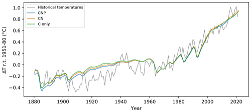
Figure 1 Historical temperature relative to 1951–1980 for the C-only, CN, and CNP model versions of the UVic ESCM compared to the GISS historical temperature dataset (GISTEMP Team, 2023).

2.2.3 Zero-emissions commitment

To explore the effects of nutrient limitation on the zero-emissions commitment (ZEC), an experiment was done following the protocol of the Zero Emissions Commitment Model Intercomparison Project (ZECMIP). The objective of the ZECMIP is to quantify the amount of unrealized temperature change after CO₂ emissions have ceased as well as the drivers behind the change (Jones et al., 2019). The experimental protocol was applied to the C-only, CN, and CNP model versions. For these experiments, the 1pctCO₂ experiment is followed until diagnosed cumulative emissions of CO₂ reach 1000 Pg C; thereafter, further CO₂ emissions are set to zero. We diagnosed three emission pathways corresponding to the C-only, CN, and CNP simulations. We used two metrics to assess the nutrient limitation effect on the ZEC. The first is the temperature at the 50th year after emissions have ceased relative to the global average temperature when emissions ceased, averaged from year 40 to year 59 after emissions cease (ZEC₅₀) as in MacDougall et al. (2020). The second is the mean ZEC for 100 years after emissions have ceased.

2.2.4 Estimated contribution of non-CO₂ climate forcings to future warming

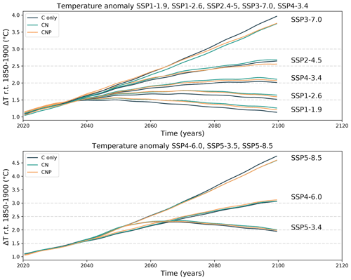
To estimate the impact of nutrient limitation on the contribution of non-CO₂ climate forcings to future warming, eight SSP scenarios for the C-only, CN, and CNP versions of the UVic ESCM (version 2.10) were run. We included the CMIP6 SSP array scenarios representing each distinct future (1–5) narrative. The following scenarios were run: SSP1-1.9, SSP1-2.6, SSP2-4.5, SSP3-7.0, SSP4-3.4, SSP4-6.0, SSP5-3.4-OS, and SSP5-8.5. The carbon budget follows temperature anomalies normalized to the 1850–1900 mean for the 1.5, 2, 2.5, and 3 °C targets. For the four overshoot scenarios (SSP1-1.9, SSP1-2.6, SSP4-3.4, and SSP5-3.4-OS), the remaining carbon budget is computed for the time at which the target is first breached.

To estimate the effect of nutrient limitation on land use change emissions and terrestrial albedo, an extra set of three simulations for the C-only, CN, and CNP model versions and the same eight SSP scenario simulations were conducted. In these simulations, land use change forcing was set to the pre-industrial value for the year 1850. The model adjusts its diagnosed CO₂ emissions to account for the missing land use change forcing. Hence, the diagnosed emission difference between the simulations with land use change forcing and without forcing corresponds to the estimated amount of land use change emissions (Mengis et al., 2018). These values also carry the effect of albedo change due to land use change. Thus, our values show the total land use change emission + albedo effect simulated in the model.

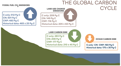
Figure 2 Simulated historical 1850–2021 cumulative land carbon sink, ocean sink, land use change emissions, and diagnosed CO₂ emissions simulated compared to Friedlingstein et al. (2022).

3 Results

3.1 Historical human-induced warming to date

For each model structure, the historical temperature was calibrated to match historical observations by altering the efficacy of aerosol forcing. Figure 1 shows the resulting near-surface air temperature anomalies for the UVic ESCM C-only, CN, and CNP configurations after calibration relative to the 1951–1980 climate normal. The temperature anomalies were plotted against the GISS near-surface air temperature anomalies relative to 1951–1980 (GISTEMP Team, 2023). For the three different versions of the model, the resulting calibrated simulations reproduced the historical temperature trend well when compared to GISS observations. As shown in De Sisto et al. (2023), the UVic ESCM CN and CNP versions without calibration have higher temperatures compared with the C-only version, given that nutrients limit the capacity of the terrestrial system to take up atmospheric CO₂. In other words, atmospheric CO₂ is higher given the same total emissions of CO₂. Between CN and CNP, CNP results in a higher temperature response, mainly as a result of tropical terrestrial nutrient limitation and extra P limitation at higher latitudes.

Figure 2 shows the historical global carbon cycle from 1850 to 2021 for the C-only, CN, and CNP model versions. There are two main impacts of nutrient limitation on terrestrial systems: (1) a reduction in the land carbon sink and (2) a reduction in the land use change emissions. The reduction in the land carbon sink is related to a decrease in the photosynthetic capacity and the regulation of terrestrial vegetation biomass. This biomass reduction leads to a reduction in the land use change emissions, especially as N and P greatly affect woody biomass. The global reduction in carbon uptake increases the concentration of CO₂ in emission-driven simulations. Following this logic and given that the concentration-driven simulations have a set atmospheric CO₂ concentration, the diagnosed emissions estimated in our simulations were reduced in CN and CNP compared with the C-only version. The model estimates that less emissions are necessary to keep the CO₂ concentration on track, as less carbon is taken up from land. In order to be comparable to the latest Global Carbon Budget report (Friedlingstein et al., 2022), estimation of the historical carbon cycle follows carbon fluxes from 1850 to 2021, while the estimation of the remaining carbon budget starts from the year 2020 following different future SSP scenario pathways. From 1850 to 2021 (Fig. 2), the range of reduction in the CN and CNP nutrient-limited simulations for the cumulative land carbon sink was 75 to 106 Pg C compared with the C-only simulation. The range of reduction in the cumulative land use change emissions was 60 to 93 Pg C. Finally, the range of reduction in the cumulative carbon emissions diagnosed by the concentration-driven simulations was 11 to 29 Pg C. The CNP cumulative fossil fuel CO₂ emission value of 483 Pg C is within the scope of the 465 ± 25 Pg C value given by Friedlingstein et al. (2022), whereas the C-only and CN values are slightly above this estimate, 501 and 512 Pg C, respectively (Fig. 2).

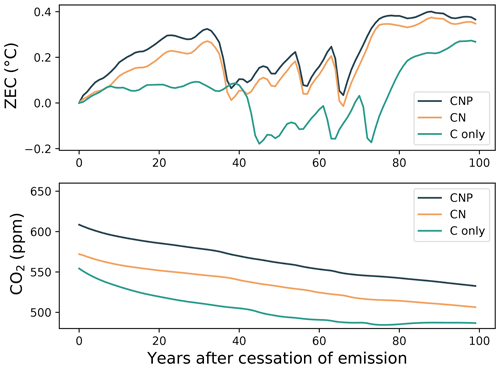
Figure 3 The zero-emissions commitment (ZEC) following the cessation of emissions during the experiment wherein 1000 Pg C was emitted following the 1pctCO2 experiment. The ZEC is the temperature anomaly relative to the estimated temperature at the year of cessation. Note that the UVic ESCM lacks internal variability. The rapid changes in global temperature seen in the top panel are due to disruptions in the ocean's meridional overturning circulation (Mengis et al., 2020).

3.2 Transient climate response to cumulative CO₂ emissions

The TCR for doubling CO₂ concentrations was 1.78, 1.79, and 1.79 °C in the C-only, CN, and CNP model versions, respectively. These small differences are driven by albedo changes. With respect to CNP and CN, the albedo change has a small increasing effect of 0.004 °C in CNP compared with CN. (Note that the UVic ESCM lacks internal variability, so this very small difference is computable.) The TCRE for the C-only version resulted in 1.74 K EgC⁻¹ compared with 1.94 K EgC⁻¹ for CN and 2.07 K EgC⁻¹ for CNP. The TCRE values for all of the simulations are within the range of 1 to 2.3 K EgC⁻¹ given by the Intergovernmental Panel on Climate Change (IPCC) Sixth Assessment Report (AR6) Summary for Policy Makers (IPCC, 2021). Under experimental conditions imposing a 1 % atmospheric CO₂ increase per year, terrestrial nutrient availability limits the capacity of terrestrial vegetation to take up carbon. Hence, even with a rapid increase in the atmospheric CO₂ concentration, the terrestrial vegetation carbon uptake capacity is limited, and the uptake rates are not as high as they would be with an unlimited amount of nutrients readily available for uptake. The effective TCRE estimated from SSP5-8.5 resulted in 1.97, 2.27, and 2.36 K EgC⁻¹ for the C-only, CN, and CNP model versions, respectively. Overall, the TCRE and effective TCRE were increased in the nutrient-limited simulations. The range of increase for TCRE was 0.2 to 0.3 K EgC⁻¹. The range of increase in the effective TCRE was 0.3 to 0.4 K EgC⁻¹. Figure 2 shows how terrestrial carbon cycle fluxes change in historical simulations. Due to these changes, the diagnosed CO₂ emissions are reduced. Hence, for any temperature target, less CO₂ emissions are required in the nutrient-limited simulations. This translates into a more sensitive model. Therefore, for 1000 Pg C emitted, the nutrient limiting simulations are going to result in higher temperatures.

3.3 Zero-emissions commitment

To analyze the impact of nutrient limitation in zero-emissions scenarios, ZECMIP-type experiments were conducted in the C-only, CN, and CNP model versions. Figure 3 shows the temperature anomaly relative to the estimated temperature at the year of cessation. The temperature pattern in the 100 years following cessation is similar for all of the model structures. There is an initial rise in temperature around the 20th year, a quick decline between the 35th and 40th year, and a subsequent increase around the 70–80th year. A difference between the C-only and the CN and CNP versions is that the C-only simulated increase is lower than the nutrient-limited simulations. The overall ZEC value is higher in CNP and CN than in the C-only simulation. Higher ZEC values indicate a larger increase in the temperature after emissions have ceased. For CN and CNP, the respective ZEC₅₀ values were 0.07 and 0.09 °C, compared with 0.02 °C in the C-only simulation. These values are similar to the ZEC₅₀ value of 0.03 °C shown in MacDougall et al. (2020) for the same model. The ZEC values across 100 years of simulation after emissions have ceased show a larger difference in temperature change after emission have ceased. The C-only simulation resulted in 0.05 °C compared with 0.17 °C in CN and 0.21 °C in CNP. This represent a relevant increase in temperature after emission have ceased in the nutrient-limited simulations.

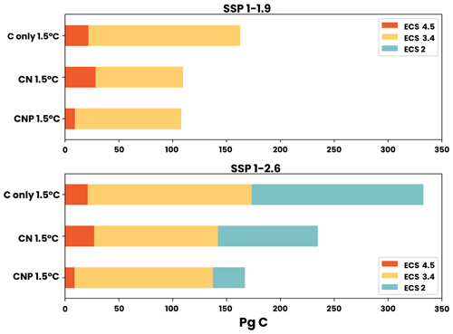
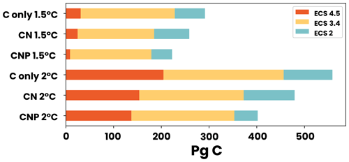
Figure 4 Carbon budgets for the 1.5 °C target for SSP1-1.9 and SSP1-2.6. The three following model sensitivities are shown: ECS 4.5 (dark blue), ECS 3.4 (green), and ECS 2 (orange).

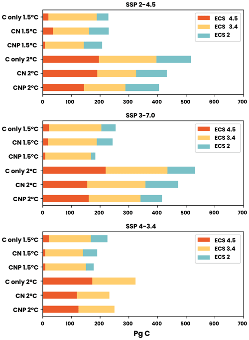
Figure 5 Carbon budgets for the 1.5 and 2 °C targets for SSP2-4.5, SSP3-7.0, and SSP4-3.4. The three following model sensitivities are shown: ECS 4.5 (dark blue), ECS 3.4 (green), and ECS 2 (orange).

Figure 6 Carbon budgets for the 1.5 and 2 °C targets for SSP4-6.0, SSP5-3.4, and SSP5-8.5. The three following model sensitivities are shown: ECS 4.5 (dark blue), ECS 3.4 (green), and ECS 2 (orange).

3.4 Estimated contribution of non-CO₂ climate forcing to future warming

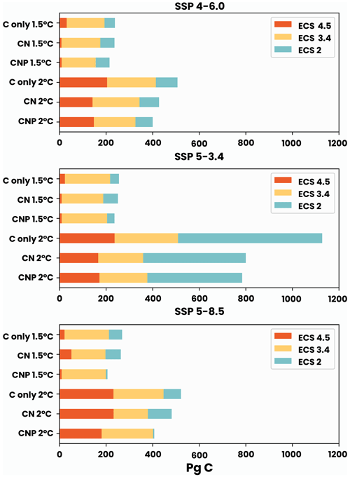
In this section, we assess the remaining carbon budget variability between different nutrient limitation model structures by employing eight SSP projections used in CMIP6. Furthermore, our focus is on portraying the role of N and P representation in remaining carbon budget estimates from different future scenarios. Figures 2–8 show the resulting remaining carbon budgets for SSP1-1.9, SSP1-2.6, SSP2-4.5, SSP3-7.0, SSP4-3.4, SSP4-6.0, SSP5-3.4, and SSP5-8.5. Among these projections, not all reached the 1.5, 2, 2.5, and 3 °C targets: SSP1-1.9 and SSP1-2.6 only reached the 1.5 °C target; SSP4-3.4 and SSP5-3.4 only reached the 2 °C target; SSP2-4.5 reached the 2.5 °C target; and SSP3-7.0, SSP4-6.0, and SSP5-8.5 reached the 3 °C target. The remaining carbon budget estimates and the SSP temperature anomalies can be seen in more detail in the Appendix (Tables A1–A3 and Fig. B1). Overall, the application of nutrient limitation increased the TCRE and, hence, decreased the carbon budget for all set targets. As expected, for the CN and CNP simulations, P limitation reduced the remaining carbon budgets. The mean remaining carbon budgets estimated among the SSP simulations for ECS 3.4 (ECS 4.5–ECS 2) in the C-only, CN, and CNP model variations for the 1.5 °C target were 228 (31–291), 185 (25–259), and 175 (9–223) Pg C, respectively. For the 2 °C target, the mean remaining carbon budget values were 471 (205–554), 373 (154–479), and 351 (137–402) Pg C for the C, CN, and CNP configurations, respectively. The remaining carbon budgets for the 2.5 °C target were 719 (378–869), 591 (321–725), and 596 (315–673) Pg C for the C, CN, and CNP configurations, respectively. Finally, the remaining carbon budgets for the 3 °C target were 974.4 (546–1174), 798 (460–986), and 796 (467–920) Pg C for the C, CN, and CNP configurations, respectively. This represents a respective CN and CNP reduction of 19 % and 24 % for the 1.5 °C target; 21 % and 26 % for the 2 °C target; 18 % and 17 % for the 2.5 °C target; and, finally, 18 % and 19 % for the 3 °C target compared with the C-only configuration.

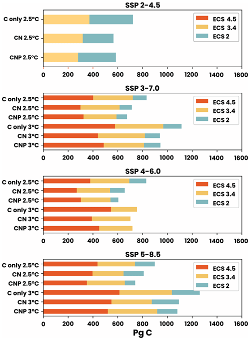
Figure 7 Carbon budgets for the 2.5 and 3 °C targets for SSP3-7.0, SSP4-6.0, and SSP5-8.5. These were the only scenarios that reached the targets. The three following model sensitivities are shown: ECS 4.5 (dark blue), ECS 3.4 (green), and ECS 2 (orange).

Figure 8 Mean SSP carbon budgets for the 1.5 and 2 °C temperature targets.

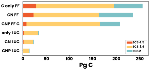
Figure 9 Mean SSP carbon budgets for fossil fuel (FF) and land use change (LUC) emissions for the 1.5 °C temperature target.

One of the impacts of nutrient limitation is the alteration of land use change emissions corresponding to the reduction and change in vegetation. We found that the mean land use change emission budgets among the SSP simulations from the year 2020 to the 1.5 °C target in the ECS 3.4 (ECS 4.5–ECS 2) were 31 (2–39), 20 (2–40), and 13 (1–23) Pg C for the C-only, CN, and CNP configurations, respectively (Fig. 9). These values corresponded to a reduction of 11.2 and 18.4 Pg C in CN and CNP compared with C-only. These results demonstrate that the remaining carbon budget is clearly sensitive to the availability of nutrients represented in SSP model simulations. As shown in Fig. 2–8, the remaining carbon budgets vary between the SSP scenarios, as temperature increases are affected by non-CO₂ forcings, corresponding to socioeconomic global uncertainties. Furthermore, in nutrient-limited cases, the land carbon cycle represents an implicit uncertainty under these different socioeconomic projections.

4 Discussion

In nature, N and P limitation or co-limitation is a core control on vegetation productivity. Hence, the inclusion of N and P limitation in ESMs improves the representation of vegetation productivity and biomass. For the UVic ESCM (version 2.10), the vegetation biomass, distribution, and productivity have been addressed in De Sisto et al. (2023), whereas the land use change emissions and albedo remained unexplored. In this study, land use change emissions account for albedo changes due to plant functional type (PFT) changes in model simulations. As the model reduces vegetation due to nutrient limitation and trees are replaced by grasses, the land surface albedo is increased. The replacement of trees by grasses occurs globally in the model, as shown in De Sisto et al. (2023). Hence, CNP and CN have a larger albedo value than C-only for land. We have identified that a terrestrial system which is stressed due to nutrient limitation reduces its land use change emission budget and increases its land surface albedo. The land surface albedo increased by 0.04 in the nutrient-limited simulations.

The terrestrial carbon cycle in nutrient-limited model structures is usually suppressed by the capacity of primary producers to uptake carbon, either (1) by controlling photosynthesis or (2) reducing the biomass directly by setting maximum nutrient ratio boundaries. In this case, terrestrial N and P act as limiting factors for terrestrial vegetation by restricting the photosynthesis (N) and by reducing the biomass given a set ratio value (N and P). N and P control biomass directly via maximum C:N or C:P leaf ratio thresholds: the lower the set ratio is, the higher the impact of nutrients. When the diagnosed C:N or C:P leaf ratios are higher than the set maximum leaf ratio, the vegetation biomass dies; thus, the leaf ratios then decrease back to the maximum ratio threshold. Nutrient limitation is also different for various PFTs; hence, the change in vegetation biomass is dependent on differences in the limitations applied to each PFT. Therefore, the application of multiple nutrient-limiting stressors, such as N and P, should be applied carefully, as high limitation of P can easily cause an underestimate of the land sink capacity of tropical vegetation. A detailed description of the terrestrial N and P uncertainties can be found in the complete description of the model in De Sisto et al. (2023).

In the CNP model version, biomass reduction goes beyond that in CN, as tropical regions are subjected to more limitations. In the UVic ESCM (version 2.10), an overestimation of broadleaf trees is found in the tropics. When P is modelled, the result is a substantial decrease in land use change emissions compared with the base version of the model, leading to a substantial difference compared with Friedlingstein et al. (2022). However, the CN configuration is still within the range shown in Friedlingstein et al. (2022).

It is clear then that the representation of the carbon cycle in the models' structures affects the estimation of the remaining carbon budgets. Permafrost thawing, for example, has been studied for its carbon budget reduction effect in ESMs (MacDougall and Knutti, 2016; MacDougall et al., 2021). In this study, the effect of the terrestrial carbon dynamics has a direct impact on the reduction in the remaining carbon budgets. The impact of N and P limitation due to a reduction in the land carbon sink should be explicitly considered to be a variable that can reduce our remaining carbon budgets for any temperature target. Furthermore, a significant number of socioeconomic uncertainties exist in the remaining carbon budget estimates, including the inability to predict future levels of carbon dioxide emissions based on sociopolitical system dynamics and technological advancements, such as those represented in the different SSP scenarios. Hence, the carbon budgets are ultimately linked to the rate of emission and the measures taken to mitigate carbon emissions in the future (Matthews et al., 2020).

The IPCC AR6 (IPCC, 2021) reports remaining carbon budget estimates from 2020 of 245, 177, 136, 108, and 82 Pg C for the 1.5 °C target with a probability of 17 %, 33 %, 50 %, 67 %, and 83 %, respectively. Compared with the 50 % probability of 136 Pg C, our nutrient-limited model simulations, CN (185 Pg C) and CNP (175 Pg C), estimated a closer value than the C-only simulation (228 Pg C). C-only tended more toward the 17 % probability value. Hence, nutrient-limited simulations bring the estimate from the UVic ESCM closer to the multi-model mean.

As shown in this study, the representation of carbon processes can affect the estimation of remaining carbon budgets in ESMs. As unrepresented processes in other models, N and P limitation reduced the estimated remaining carbon budget in the respective CN and CNP configurations by 43 and 53 Pg C for the 1.5 °C target and by 98 and 120 Pg C for the 2 °C target when compared with the C-only simulation. These estimations are larger than the rough estimate of a 27 Pg C reduction in the carbon budget due to unrepresented carbon feedbacks (Rojelj et al., 2018), suggesting that this value may have been underestimated in the IPCC 1.5 °C report.

The TCRE shows that N and P limitation has a direct effect on the temperature-to-carbon emission proportionality. Nutrient limitation impacts the carbon fluxes, reducing the land carbon sink and increasing the ocean carbon sink, ultimately leading to a net decrease in carbon uptake from the land and ocean. In emission-driven simulations, this will lead to a high build-up of atmospheric CO₂. However, it is clear that a deeper understanding of the nutrient distribution is necessary to build even more reliable nutrient-limited models. Effort should be directed towards the creation of reliable data, including data on the global nutrient distribution; global nutrient inputs; and future fertilization projections encompassing agriculture and human waste load into terrestrial, riverine, and aquatic systems.

In ESMs, nutrient simulations could be improved via the inclusion of further global observations. The current available data have large ranges and make it difficult to assess the reliability of the nutrient values given by ESM simulations. Theses uncertainties are present in most aspects of the global N and P cycles. Hence, it is hard to grasp how accurate our model outputs are in comparison with nature. This is especially true for P, which lacks more observational datasets compared with N. Despite the uncertainty rooted in N and P models and projections, it is clear that nutrient limitation reduces the remaining carbon budgets by constraining the vegetation capacity in terrestrial ecosystems. Our results only show the effect of nutrient limitation in one model structure. The response of Earth system models to nutrient limitation varies amongst models depending on how terrestrial N and P limitations are applied. Furthermore, although we may capture some of the range shown in other models by varying the ECS, the full range of structural uncertainty is not captured by our experimental design.

The inclusion of P in ESMs and the benefits of CNP models have been shown to improve the accuracy of the terrestrial carbon cycle (Wang et al., 2010; Goll et al., 2017; De Sisto et al., 2023). However, the necessity to include P in models' structures is debatable. If the objective is to improve the carbon cycle accuracy, the inclusion of P is advisable due to its limiting role in tropical regions. From a carbon budget estimation point of view, we observed similar results for the CN and CNP configurations. Overall, our results show that remaining carbon budgets estimated in CNP simulations were lower than those in CN configurations. SSP projections where this was not the case match those scenarios representing a medium to high implicit land use regulation. Hence, one of the main differences between CN and CNP models is how the model responds to land use change management in different future projection scenarios. The inclusion of P in ESMs has been shown to improve the terrestrial model performance; hence, we believe that the addition of P limitation should be considered in the development plans of different model working groups.

5 Conclusion

Remaining carbon budgets are crucial for climate policy and management. As the remaining carbon budgets are intrinsically linked to the TCRE and the dynamics of the global carbon budget, it is important to consider the uncertainties that nutrient limitations impose on our terrestrial model structures. In this study, we found that nutrient limitation, in this case N and P limitation, had a considerable effect on the remaining carbon budget estimates. Historically, N and P limitation reduced the land carbon sink and land use change emissions. The range of reduction in the land carbon sink was 75 to 106 Pg C, while the range of reduction in the land use change emissions was 60 to 93 Pg C. Overall, under the SSP projections, N and P reduced the remaining carbon budget estimates for the 1.5, 2, 2.5, and 3 °C targets. The respective CN and CNP model versions showed a reduction of 43 and 53 Pg C for the 1.5 °C target and 98 and 120 Pg C for the 2 °C target when compared with the C-only configuration. Theses values represent a reduction of 19 % and 24 % for the 1.5 °C target and 21 % and 26 % for the 2 °C target for CN and CNP, respectively. After emissions had ceased, N and P had a relevant impact on the temperature change: the ZEC across 100 years of simulation after emissions had ceased showed a 0.12 and 0.16 °C increase in temperature for the CN and CNP nutrient-limited simulations, respectively, when compared to C-only. The uncertainty in the magnitude of the reduction in the remaining carbon budget due to nutrient limitation would be more clear if a multi-model assessment was conducted. Overall, we assess that accounting for nutrient limitations would lead to a substantial reduction in the estimated remaining carbon budget.

Appendix A

Table A1 Remaining carbon budgets from the SSP2-4.5, SSP3-7.0, and SSP4-3.4 simulations for the 1.5 and 2 °C targets relative to a warming from 1850 to 1900.

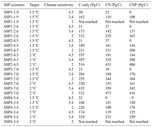
Table A2 Remaining carbon budgets from the SSP4-6.0, SSP5-3.4, and SSP5-8.5 simulations for the 1.5 and 2 °C targets relative to a warming from 1850 to 1900.

Table A3 Remaining carbon budgets from the SSP-2.45, SSP3-7.0, SSP4-6.0, and SSP5-8.5 simulations for the 2.5 and 3 °C targets relative to a warming from 1850 to 1900.

Appendix B: Temperature anomalies of the SSP simulations for C-only, CN, and CNP

Figure B1 The SSP temperature anomalies relative to 1850–1900 for the C-only, CN, and CNP simulations.

Appendix C: Above-ground terrestrial vegetation biomass

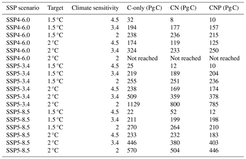
Figure C1 shows the above-ground vegetation representation in the UVic ESCM (version 2.10) with terrestrial N and P limitation. The main differences are shown to be located in tropical regions. The model both underestimates (forests in the Amazon, Borneo, and Indonesia) and overestimates (forests in Brazil, Venezuela, Colombia, Central America, sub-Saharan Africa, and part of Southeast Asia) above-ground vegetation biomass in tropical regions, in comparison with Santoro et al. (2024). However, the values estimated by the model with and without nutrients are shown to be within the range of uncertainty of literature values (Mengis et al., 2020; De Sisto et al., 2023).

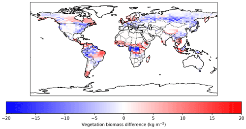
Figure C1 Above-ground vegetation biomass difference between the UVic ESCM CNP (version 2.10) and Santoro et al. (2024) ESA CCI Biomass product datasets for the years 2017–2018.