the Creative Commons Attribution 4.0 License.
the Creative Commons Attribution 4.0 License.
 | 02 Feb 2024
Central Arctic Ocean surface–atmosphere exchange of CO2 and CH4 constrained by direct measurements
Sonja Murto
Ian Brown
Adam Ulfsbo
Brett F. Thornton
Volker Brüchert
Michael Tjernström
Anna Lunde Hermansson
Amanda T. Nylund
Lina A. Holthusen
The central Arctic Ocean (CAO) plays an important role in the global carbon cycle, but the current and future exchange of the climate-forcing trace gases methane (CH4) and carbon dioxide (CO2) between the CAO and the atmosphere is highly uncertain. In particular, there are very few observations of near-surface gas concentrations or direct air–sea CO2 flux estimates and no previously reported direct air–sea CH4 flux estimates from the CAO. Furthermore, the effect of sea ice on the exchange is not well understood. We present direct measurements of the air–sea flux of CH4 and CO2, as well as air–snow fluxes of CO2 in the summertime CAO north of 82.5∘ N from the Synoptic Arctic Survey (SAS) expedition carried out on the Swedish icebreaker Oden in 2021.
Measurements of air–sea CH4 and CO2 flux were made using floating chambers deployed in leads accessed from sea ice and from the side of Oden, and air–snow fluxes were determined from chambers deployed on sea ice. Gas transfer velocities determined from fluxes and surface-water-dissolved gas concentrations exhibited a weaker wind speed dependence than existing parameterisations, with a median sea-ice lead gas transfer rate of 2.5 cm h−1 applicable over the observed 10 m wind speed range (1–11 m s−1). The average observed air–sea CO2 flux was −7.6 , and the average air–snow CO2 flux was −1.1 . Extrapolating these fluxes and the corresponding sea-ice concentrations gives an August and September flux for the CAO of −1.75 , within the range of previous indirect estimates.
The average observed air–sea CH4 flux of 3.5 , accounting for sea-ice concentration, equates to an August and September CAO flux of 0.35 , lower than previous estimates and implying that the CAO is a very small (≪ 1 %) contributor to the Arctic flux of CH4 to the atmosphere.
- Article
(3586 KB) - Full-text XML
-
Supplement
(4106 KB) - BibTeX
- EndNote


The Arctic is on average warming up to 4 times faster than the global average rate (Rantanen et al., 2022), manifested in dramatic reductions in sea-ice extent (Onarheim et al., 2018) and thickness (Kwok, 2018). Reduced sea-ice cover in a warming Arctic is expected to have complex effects on air–sea gas exchanges (Parmentier et al., 2013), in particular for the exchange of the two gases whose rising atmospheric concentrations are principally responsible for the observed global warming, carbon dioxide (CO2) and methane (CH4). The parameterisation of gas transfer in the presence of sea ice is still under debate but is expected to have large impacts on polar carbon budgets: for example, Arctic Ocean CO2 uptake estimates are highly dependent on the parameterisation choice, with resulting uptake differences of 50 Tg C yr−1, i.e. ∼ 30 % of the total (Yasunaka et al., 2018). The Arctic Ocean corresponds to 5 %–14 % of the global ocean CO2 sink from 3 % of the global ocean area (Bates and Mathis, 2009; Yasunaka et al., 2016, 2018).
The central Arctic Ocean's (CAO) role in carbon cycling and the exchange of climate-forcing trace gases with the atmosphere is uncertain due to several factors, including limited observations of dissolved gas concentrations and air–sea fluxes. The CAO is defined as the deep-water part of the Arctic Ocean, excluding the shallow shelf seas (Jakobsson, 2002). Thus defined, the CAO has an average depth of 2748 m and an area of 4.5 × 10⁶ km2, which corresponds to about 47 % of the surface area of the entire Arctic Ocean.
Sources of CH4 from the Arctic Ocean are poorly constrained and spatially variable (Thornton et al., 2016a). Oceans have long been seen as generally a weak source of CH4. The shelf seas of the Arctic and particularly the extensive shallow East Siberian Shelf are believed to be a large source, though are poorly constrained. Here, with potential sources of CH4 from thawing subsea permafrost and riverine input (Weber et al., 2019; Manning et al., 2020), fluxes of 9–286 were observed with direct measurement (Thornton et al., 2020), and 187–238 were estimated from seawater concentrations (Thornton et al., 2016b). While the integrated magnitude of these Arctic marine methane emissions remains under debate, it appears to presently be on the scale of ∼ 4–5 Tg CH4 yr−1 or 100 (Thornton et al., 2016a, b, 2020), i.e. ∼ 1 % of global CH4 emissions (Saunois et al., 2020). There are previously no direct CH4 flux measurements available from the CAO. The estimates that are available are derived from near-surface (typically ∼ 10 m depth) concentrations (Manning et al., 2022; Damm et al., 2018; Fenwick et al., 2017; Lorenson et al., 2016). Seawater CH4 measurements from the North American Arctic shelf and Canada Basin suggest small fluxes of 0.3–2.2 (Manning et al., 2022; Fenwick et al., 2017). Excess CH4 may be transported from shallow sea areas across the Arctic Ocean in the water column and also frozen in sea ice and in brines within the ice (Damm et al., 2018). Seawater CH4 concentrations from the Beaufort Shelf and CAO were used to estimate an Arctic-wide CH4 flux of 7.5 and a potential flux, if the ice disappeared from currently ice-covered areas, of 18–63 (Lorenson et al., 2016). Emissions of CH4 derived from changing seawater concentrations following a winter storm ∼ 150 km north of Svalbard were 19 during the storm and 5 afterwards (Silyakova et al., 2022). Much higher fluxes (125 ), extending for at least 50 km over wintertime (November and April) sea-ice leads at latitudes up to 82∘ N, have been derived from aircraft-based atmospheric profile measurements (Kort et al., 2012). These fluxes, observed over deep water, are ascribed to local CH4 production associated with the mixed sea ice and lead environment. The large range of indirect estimates of CAO CH4 emissions presents a challenge to modelling and highlights the need for direct measurements.
The CAO is generally undersaturated with respect to atmospheric CO2. This undersaturation is due to a combination of the low temperatures and resulting lower gas saturation, dilution due to freshwater input, limited atmospheric equilibration due to the presence of sea ice, CaCO3 dissolution (Fransson et al., 2017), vertical mixing and primary production, particularly in shelf seawater advected to central areas (Bates et al., 2006). Average Arctic Ocean uptake in summer months, with a sea-ice concentration (SIC) of ∼ 50 % and a CO2 partial pressure (pCO2w) undersaturation of ∼ 80 µatm, is estimated at −4 (Yasunaka et al., 2018). The majority of existing Arctic Ocean observations are from coastal regions, with average air–sea fluxes in the eastern Arctic Ocean of 0–10 (Manizza et al., 2019) and average air–sea fluxes in the western Arctic Ocean somewhat higher at 0–20 , primarily due to low SIC in the Chukchi Sea (Bates and Mathis, 2009; Ouyang et al., 2022). In the CAO, observations of pCO2w and the air–sea flux are especially sparse. Yasunaka et al. (2018), using a self-organising map to extrapolate the sparse near-surface CO2 observations, determine the mean flux for the CAO region to be below the uncertainty in their method (uncertainty 2.8 to 3.7 ). Coupled ocean–biogeochemistry modelling gives an annual CAO flux of −2.2 ± 4.0 Tg CO2 yr−1 (Manizza et al., 2019). Earlier estimates from the Canada Basin suggested fluxes smaller than −3 in periods with SIC near 100 % but an uptake of around −55 in summer months, with lower SIC (Bates et al., 2006). High fluxes can occur when water undersaturated with CO2, high winds and open-water coincide, with CO2 fluxes of up to −86 estimated in June close to the pack edge north of Svalbard (Fransson et al., 2017). Fluxes determined from direct, eddy covariance measurements in areas adjacent to ice or from lead water surfaces are of the order of −10 , in both central and coastal areas of the Arctic Ocean (Prytherch et al., 2017; Dong et al., 2021; Prytherch and Yelland, 2021).
The presence of sea ice makes the Arctic Ocean a highly heterogenous and dynamic environment over a wide range of spatial scales, complicating robust model representation of surface exchange processes. Wind speed is the primary forcing of gas exchange in the ice-free ocean (Wanninkhof et al., 2009). Sea ice limits air–sea gas exchange but also contributes to its forcing through additional sea-ice-dependent physical processes that impact interfacial mixing. This implies a non-linear relationship of gas transfer rate to sea-ice cover (Loose et al., 2014). The highest rates of gas exchange in pack ice regions occur through open-water areas such as leads. Leads appear on scales from < 1 m to > 10 km and can open, change size and close throughout all seasons (Marcq and Weiss, 2012). Sea-ice-dependent processes impacting gas exchange from lead surfaces are shear between floating ice and the underlying water (Lovely et al., 2015), upper-ocean stability, stratification from freshwater during ice melt and convection-driven turbulent mixing from surface buoyancy during freeze periods (MacIntyre et al., 2010). Also, modifications to the wind stress input from ice-edge form drag, ice–wave interactions and short fetch conditions (Bigdeli et al., 2018). Direct ship-based eddy covariance measurements support an inverse linear scaling of exchange with SIC (Butterworth and Miller, 2016; Prytherch et al., 2017), while laboratory and indirect radon isotope measurements support an enhanced exchange (Fanning and Torres, 1991; Loose et al., 2011, 2017). Recent direct and indirect gas exchange observations suggest that gas exchange will be reduced in the presence of sea ice (Rutgers van der Loeff et al., 2014; Prytherch and Yelland, 2021).
Strong, near-surface gradients in dissolved gas concentrations are prevalent in Arctic sea-ice regions (e.g. Miller et al., 2019; Ahmed et al., 2020; Dong et al., 2021). Unaccounted for, this stratification will bias flux estimates and parameterisations of gas transfer derived from sub-surface concentrations. Using eddy covariance (EC) flux measurements, Dong et al. (2021) showed that surface fCO2 in the summertime Arctic marginal ice zone was 39 µatm lower than that measured from their ship's intake at 6 m depth. They determined that this was partly due to the effects on CO2 solubility from meltwater cooling and freshening, with approximately half of the reduction from other factors, presumably photosynthesis. Miller et al. (2019) report pCO2w differences between the surface and an intake at 7 m depth of between −180 and +160 µatm during sampling in the Canadian Arctic Archipelago and Hudson Bay. The authors note that “The temperature differences between the underway system and the shallower samples were often contrary to the pCO2 gradients …, indicating that pCO2 was not simply controlled by surface heating and cooling”. Due to surface longwave emission and the resulting cool-skin effect (Woolf et al., 2016), temperature differences are always present between the sea surface and intake depths even when the upper ocean is well mixed.
Sea-ice can be porous due to brine channels within the ice and can exchange gases with the atmosphere (Delille et al., 2014). Ice–atmosphere fluxes of CO2 are typically smaller than those through water surfaces (on the order of 1 ) but can be a significant contributor to regional fluxes in sea-ice areas. Ice–atmosphere fluxes are largely dependent on temperature (Delille et al., 2014) and snow cover thickness (Geilfus et al., 2012; Nomura et al., 2010). Ice–atmosphere CH4 fluxes are less well known. Sea-ice cores obtained on the Siberian shelf have been supersaturated with CH4, while cores from the CAO were close to equilibrium, but atmospheric fluxes were not determined (Damm et al., 2015). There are no reported measurements of ice–atmosphere CO2 or CH4 flux in the summertime CAO.
The high sensitivity and small footprint of the flux chamber technique makes it attractive for measurements in small waterbodies such as leads. The technique has been frequently used in inland waterbodies but is criticised because the chamber isolates the air–water interface from the wind and may modify the gas exchange process. While this isolation suggests that chambers reduce gas transfer, previous studies have often suggested an overestimation of k when determined from chambers, resulting from artefact turbulence at the water surface introduced by the chamber, particularly at very low wind speeds (Matthews et al., 2003; Vachon et al., 2010). The gas transfer of poorly soluble gases is controlled by mixing on the water side of the interfacial layer, and the mixing itself depends on forcings such as wind speed (Wanninkhof et al., 2009). If water is able to advect into the chamber rapidly and with minimal modification by the chamber, then the gas transfer within the chamber will be representative of the outside environment. Appropriate chamber designs with minimal penetration into the water layer, high surface-to-volume ratios and short measuring intervals minimise such measurement bias.
To remedy some of the uncertainties reviewed above we here report direct measurements of the air–sea flux of CO2 and CH4, gas transfer velocities determined from the air–sea flux measurements and surface-water-dissolved gas concentrations, and air–snow fluxes of CO2 during the period of rapid sea-ice melt in the summertime CAO. We relate the gas transfer velocities to wind speed and lead width, discuss the measurement uncertainties and estimate regional CAO fluxes.
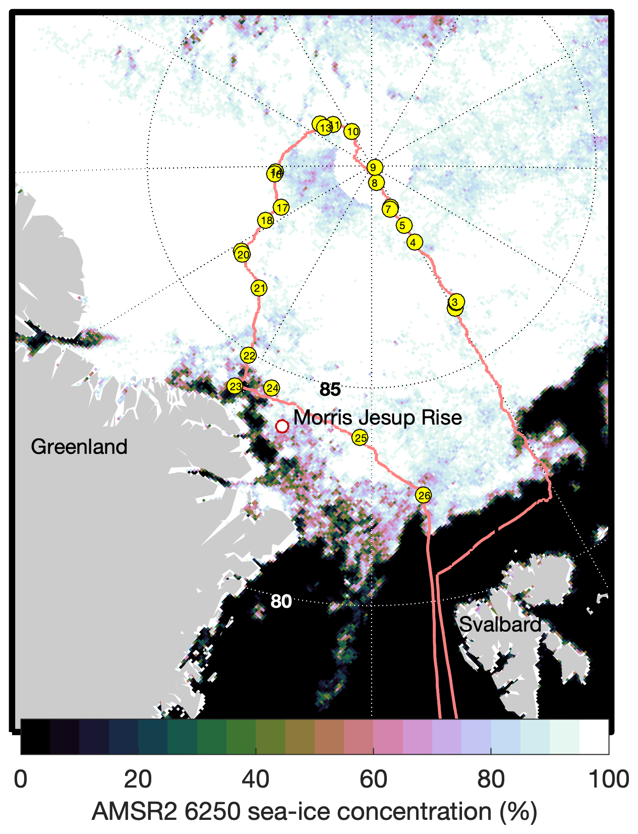
Figure 1Map of the expedition route (red line) with chamber flux sampling locations (yellow circles) and numbers corresponding to Table S1. Sea-ice concentration is shown as determined for 1 September 2021 by AMSR-2 satellite observations and the ASI 6.25 km2 product.
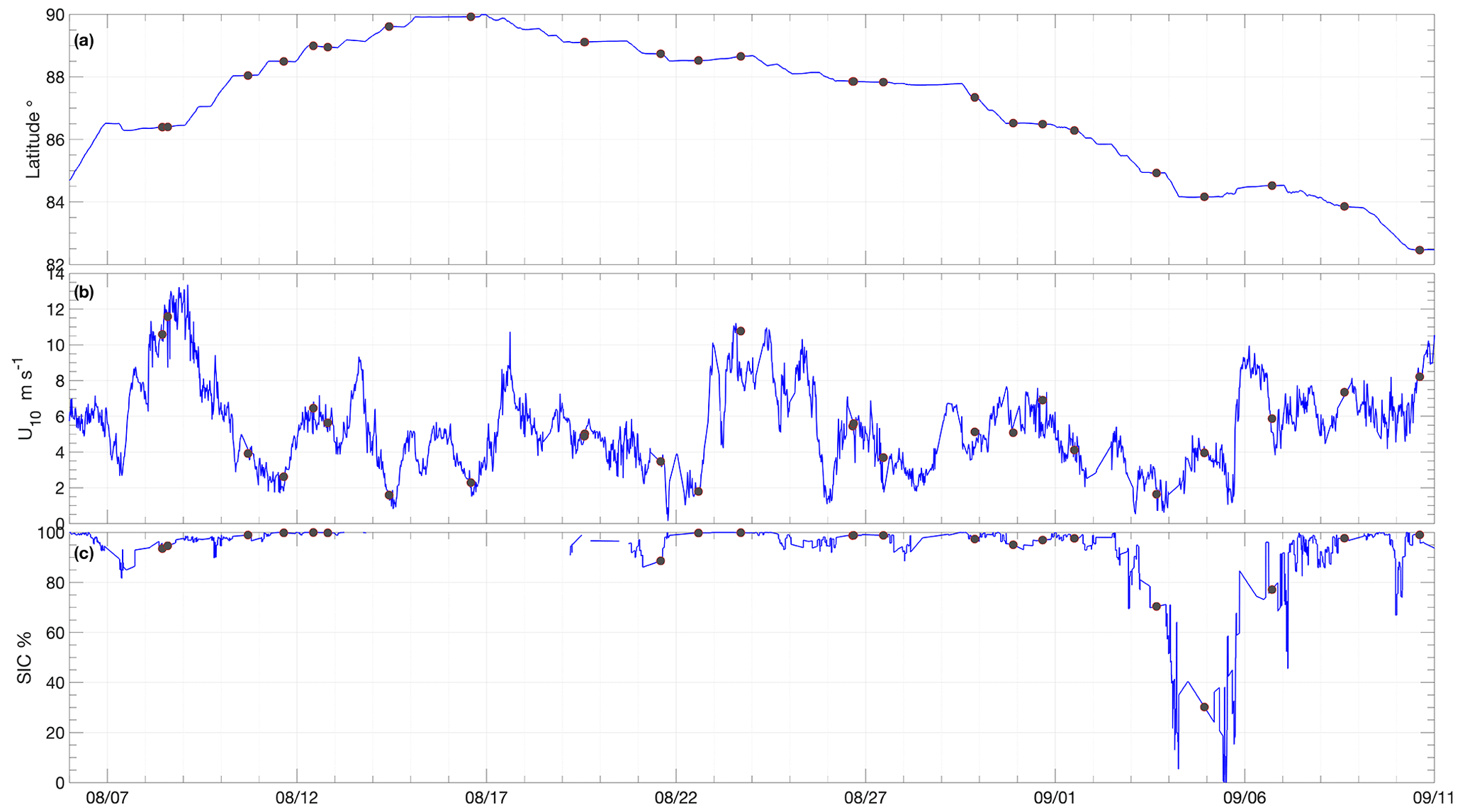
Figure 2Time series of (a) Oden's latitude, (b) wind speeds as measured on Oden and (c) SIC determined from the ASI 6.25 km2 product interpolated to Oden's position. Grey circles in each plot show averaged values corresponding to the times of flux chamber measurement.
Measurements were obtained during the Synoptic Arctic Survey (SAS) expedition (Snoeijs-Leijonmalm et al., 2022) carried out on the Swedish icebreaker Oden in 2021. The science operations of the expedition began on 1 August, when Oden reached the ice edge north of Svalbard (80.71∘ N, 11.20∘ E). Oden transited to the North Pole along 30∘ E, then towards the northern coast of Greenland along the Lomonosov Ridge and then east from the Morris Jesup Rise towards Svalbard, with relevant science operations finishing on 11 September (Figs. 1 and 2a).
Ice stations were carried out throughout the expedition during which Oden halted in the ice for periods ranging between several hours and 2 d in order to perform winch operations such as conductivity–temperature–depth (CTD) sensor and Niskin bottle casts and net deployments. During long-duration stations, sampling was carried out directly from the sea ice at locations within a radius of ∼ 200 m of Oden or to a radius of ∼ 500 m using Oden's helicopter. During shorter stations where on-ice work was not possible, measurements were performed from over the side of the ship (overside).
2.1 Gas flux measurements
Measurements of the air–water CO2 and CH4 flux were made using floating chambers (e.g. Cole et al., 2010). Two types of floating chamber sampling were performed: ice-based sampling, with the chamber placed onto lead water or melt pond surfaces accessed from sea ice and allowed to float freely, and overside sampling during the shorter stations, with the chamber lowered over Oden's side to the water surface, resulting in sampling closely adjacent to the ship. Fluxes measured overside may be influenced by the presence of Oden impacting the gas exchange rate both through modification of the near-surface winds and through modification of ocean near-surface turbulence. Measurements were made as far from any propeller movement or water flushing as possible but there may still have been some influence on the measurements. In the presence of upper-ocean dissolved gas concentration gradients, mixing induced by Oden may modify the air–sea concentration difference that drives the flux. As such, overside and ice-based flux and surface water gas concentration measurements are presented separately throughout this study.
Two floating chamber flux systems were used during SAS, both comprising a gas analyser and air pump connected through tubing in a closed loop with the chamber. The first system used a Los Gatos Research (LGR) greenhouse gas analyser cavity-enhanced laser spectrometer, measuring mixing ratios of CO2, CH4 and H2O. The second system used a Li-COR 7200RS non-dispersive infrared (NDIR) spectrometer, measuring CO2 and H2O mixing ratios. Surface fluxes of a gas species are determined from the gradient with time of the gas mixing ratio in the chamber, with an approximately linear gradient required for a successful flux measurement. The sampling time for each flux measurement was approximately 10 min, after which the chamber was manually raised from the surface and equilibrated with atmosphere, before being replaced to begin the next sampling period. Each chamber deployment during SAS typically consisted of circa eight sampling periods (from 2 to 10). The mean of the fluxes measured within each deployment is used in the subsequent analysis, with the standard error in fluxes indicating the variability within each deployment. Fluxes were converted to using the chamber surface area, the volume of the total chamber system (chamber, tubing and analyser measurement cell), chamber air pressure and the ideal gas law.
The same chambers were used with both analysers. The chambers are custom built, consisting of upturned polyethylene bowls, with foam floats attached and rubber stoppers in the roof through which the tubing is inserted (Fig. S1 in the Supplement). The chambers are lightweight and low profile (volume 7489 mL, surface area 0.078 m2), have small chamber wall intrusion depths (< 3 cm), and are allowed to float freely. Wind is the dominant source of surface mixing energy in the open ocean and most large waterbodies. Chamber flux measurement necessarily involves isolation of an area of water from the wind. The chamber design and sampling choices are made to minimise known measurement biases resulting from anchoring effects (Lorke et al., 2015) and from chamber size and shape and sampling duration (Matthews et al., 2003; Mannich et al., 2019). Similar chamber designs to that deployed here have been shown to determine gas exchange rates in agreement with those determined in streams and small lakes from tracer releases (Cole et al., 2010), surface dissipation measurements and IR (infrared) imagery (Gålfalk et al., 2013). With appropriate flux chamber design (i.e. the relatively small and lightweight chambers used here), it is assumed that the wind-induced interfacial layer mixing, the controlling factor for air–sea gas transfer of poorly soluble species, is advected within the chamber with minimal modification of the mixing by the chamber.
Air–snow CO2 flux measurements were made using a PP Systems CPY-4 chamber connected to an EGM-4 NDIR analyser and mixed by a fan inside the chamber (e.g. Miller et al., 2015). The transparent chamber (volume 2344 mL, surface area 167 cm2) was covered to minimise insolation effects and deployed on undisturbed snow surfaces. The chamber collar was pressed 1 cm into snow to prevent air leaks. The sampling time was also 10 min here.
Measurements of surface atmosphere CO2 and CH4 flux were also made throughout the expedition by EC from a system installed on Oden's foremast (Prytherch et al., 2017). Post-cruise analysis determined that fluxes measured in sea-ice regions were below the limit of detection of this system. While the strong observed CO2 undersaturation resulted in air–sea fluxes at the lead spatial scale that would be within the typical detectable range of EC systems, the high sea-ice concentration within the EC footprint (of approximately square kilometre scale from the 20 m EC measurement height) throughout the expedition substantially reduced the signal size (e.g. Prytherch et al., 2017), and as such EC measurements are not used in the analysis here (see the Supplement).
Throughout this paper we use the convention that positive fluxes are upwards, i.e. indicating a release of gas from the surface to the atmosphere, and negative fluxes are a downwards flux, indicating uptake of gas by the surface from the atmosphere.
2.2 Water sampling
On board Oden, an underway seawater intake system continuously pumped water from a depth of approximately 8 m. Water temperature at 8 m depth was measured close to the underway line inlet with two hull contact sensors, and the temperature and salinity of the underway line water were measured using a Seabird SBE45 thermosalinograph (TSG) located in Oden's main lab. Downstream of the TSG on the underway line, a Pro Oceanus CO2-Pro CV membrane equilibration sensor measured the equilibrated CO2 mixing ratio from which pCO2w was calculated. This sensor was factory-calibrated prior to the expedition and performed an automated zeroing procedure every 6 h. The manufacturer states the accuracy to be ± 3 ppm.
Surface water was sampled during the expedition to determine dissolved gas concentrations and carbonate system variables. Water samples were taken using bottles submerged at depths of 0–10 cm and using syringes at depths of 0–5 cm. During some stations a Ruttner sampler was used to obtain water samples at depths from 0.5 to 2.5 m. During overside chamber flux sampling, water samples were obtained using a lowered bucket, with the resulting water depth range for bottle and syringe samples corresponding approximately to the height of the bucket (0–30 cm). Temperature and practical salinity during each sampling were measured with a WTW 340i conductivity probe. Discrete sampling at depth and from the underway line followed the washing and repeat overflow protocols described in Dickson et al. (2007). For surface water bottle sampling, the bottles were first washed with seawater and then submerged by hand gradually while lying sideways to minimise air–water mixing, as it was not possible to follow standard overfilling protocols (Dickson et al., 2007). Syringe sampling is not described in the carbon system sampling protocols but follows Bastviken et al. (2003). The syringes were repeatedly washed with seawater prior to sampling.
Samples of dissolved inorganic carbon (DIC) and total alkalinity (TA) were collected in Pyrex® borosilicate bottles (250 mL) according to Dickson et al. (2007), without being poisoned with mercury chloride (HgCl2). Samples were stored short-term (typically less than 12 h, +4 ∘C and dark) and thermostated to 25 ∘C in a water bath prior to analysis. DIC was determined using a coulometric titration method based on Johnson et al. (1987) with a modified single-operator multiparameter metabolic analyser (SOMMA) system (coulometer type UIC 5012), and the mean difference and standard deviation of duplicate sample analysis were 5.0 ± 2.5 µmol kg−1 (n=12). TA was determined using a semi-open-cell potentiometric (Orion ROSS 8102BN) titration (Metrohm Dosimat 665) method using a five-point Gran evaluation (Haraldsson et al., 1997), and the mean difference and standard deviation of duplicate sample analysis were 3.4 ± 2.5 µmol kg−1. The accuracy in DIC and TA was ensured by routine analysis of certified reference material (CRM Batch no. 181 and no. 191) obtained from Andrew G. Dickson of Scripps Institution of Oceanography (La Jolla, CA, USA). The pCO2w was calculated from measured DIC and TA using the CO2SYSv1.1 MATLAB toolbox (Lewis and Wallace, 1998; van Heuven et al., 2011) and the dissociation constants of Lueker et al. (2000).
Samples for CH4 analysis from surface leads, buckets, CTD and the pumped underway line were collected into 500 mL borosilicate bottles. Bottles were allowed to overfill with the bottle volume three times to remove gas bubbles, poisoned with 100 µL of saturated HgCl2 and then transferred to the laboratory. Prior to analysis, samples were placed into a water bath at 25 ∘C and thermostated for a minimum of 2 h before analysis. All samples were analysed within 3 d of collection. Samples were analysed by single-phase equilibration gas chromatography (GC) using a flame ionisation detector (FID), similar to that described by Upstill-Goddard et al. (1996). Samples were calibrated against three certified ± 5 % reference standards, which are traceable to NOAA WMO-CH4-X2006A. Concentrations in seawater at equilibration temperature (∼ 25 ∘C), in situ salinity and dissolved partial pressures of CH4 (pCH4w), were calculated using the ideal gas law, Henry's law and CH4 solubility determined by Wiesenburg and Guinasso (1979).
Additional water samples were collected with 60 mL PVC plastic syringes, where 30 mL of seawater was equilibrated with 30 mL air immediately after sampling, and the equilibrated air sample stored as headspace in 20 mL vials that were prefilled without headspace with a saturated NaCl solution (Bastviken et al., 2003). The headspace gas was analysed after the expedition using the methods described in Lundevall Zara et al. (2021) and determined on an SRI 8610 GC with FID and methaniser. Headspace concentrations were corrected for the atmospheric background of CH4 and CO2 determined with the LGR gas analyser, accounting for the soluble fraction in the equilibrated 30 mL water sample, and pCO2w and pCH4w were calculated. The precision of replicate equilibration samples was 5 % or better.
For each sampling time and location, the bottle- and syringe-derived measurements were combined to obtain an average time series of both surface pCH4w and surface pCO2w, with measurement uncertainty given as the standard error of the mean (the range between the bottle and syringe values is equivalent to twice the standard error). A comparison of the measurements obtained from the different sampling methods and further details of the averaging process are given in Sect. 1 and Fig. S2 in the Supplement.
2.3 Meteorological and sea-ice measurements
Meteorological measurements were made on board Oden using a semi-permanent suite of instrumentation (Vüllers et al., 2021). Wind speed and direction was measured on the foremast at 20 m height, corrected for airflow distortion (Prytherch et al., 2017) and adjusted to 10 m height assuming a logarithmic profile and neutral stability conditions, which are prevalent in the summertime CAO. For winds coming from behind Oden (more than 90∘ from bow on), mast measurements were replaced with those from anemometers mounted at each side of the bridge roof at 28 m height, which were also corrected for height but not airflow distortion. All wind measurements are given as ice-relative speeds. Air temperature and humidity were measured on the foremast at 20 m height with aspirated sensors. Surface temperature was determined as the average measurement of two KT15.IIP infrared sensors mounted on each side of the bridge roof at 25 m, observing the surface approximately 30 m to port and starboard of Oden's hull. Snow and ice surface temperatures were additionally measured adjacent to snow/ice flux sampling using thermistors inserted into the upper few centimetres of the snow or ice surface. Lead widths and other distances were measured with a laser rangefinder (Naturalife PF4). Sea-ice thickness and freeboard were determined adjacent to ice flux sampling sites as the average from three 2 cm auger-drilled holes.
Surface buoyancy flux into lead waters was determined following MacIntyre et al. (2009) using the net radiative fluxes and turbulent heat fluxes made on board Oden (Vüllers et al., 2021) and water surface temperature and salinity. Turbulent fluxes were gap-filled using the bulk estimates (Smith, 1988).
2.4 Gas transfer velocity calculation
The air–sea flux, FX, of a poorly soluble gas species X, such as CO2 and CH4, can be represented as (e.g. Wanninkhof et al., 2009; Fairall et al., 2022)
where K0X is the aqueous-phase solubility of X () and ΔfX is the difference in the fugacity of X between the surface water and air. Fugacity is partial pressure corrected for non-ideality: this correction is very small (< 1 %) for CO2 and CH4 in summertime Arctic conditions (McGillis and Wanninkhof, 2006), and partial pressures are used in all calculations reported here. The gas transfer velocity, k, represents the kinetic forcing of the flux, dependent on both molecular diffusivity, D, water viscosity, ν, and processes that impact transfer across the water surface interfacial layer. To account for the dependence of diffusivity on gas species, temperature and salinity, k is commonly normalised in terms of the non-dimensional Schmidt number Sc ():
Here, 660 is the Schmidt number of CO2 in seawater at 20 ∘C, and the exponent n depends on the hydrodynamics of the interfacial layer and is commonly chosen to be 0.5 for a wavy surface (e.g. Jähne et al., 1987).
We determine k660 from Eqs. (1) and (2) using measurements of FX from the floating chamber and measured partial pressure differences and solubilities and Sc calculated from the polynomial relationships summarised in Wanninkhof (2014), with the solubility relationships for CO2 and CH4 originally determined by Weiss (1974) and Wiesenburg and Guinasso (1979), respectively. Uncertainties in k660 are determined from a combination of the flux and surface water partial pressure standard errors. Where the partial pressure comprised only one sample and so had no error value, the mean partial pressure standard error for that species is used instead.
Unless otherwise stated, data are presented as means and standard deviations. The air–water fluxes and coincident supporting measurements are shown in Table S1 in the Supplement, and air–ice and air–snow fluxes are shown in Table S2 in the Supplement. The uncertainties in the flux measurements shown in the tables and figures are the standard error of the samples within each chamber deployment, and the uncertainties in the surface partial pressures in Table S1 and the figures are the standard error of the samples comprising each measurement.
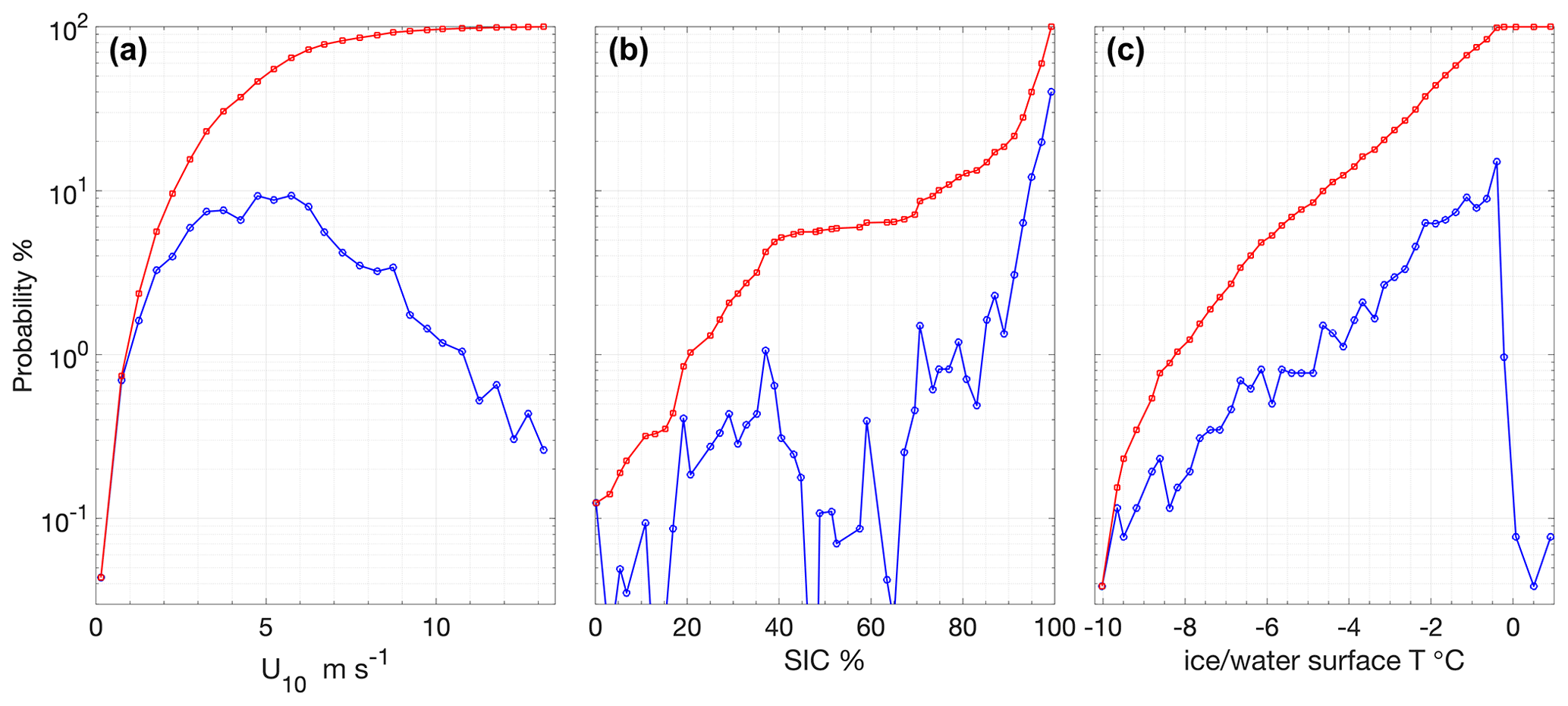
Figure 3Occurrence probability (blue) and cumulative probability (red) during the expedition of (a) wind speeds adjusted to 10 m height, (b) SIC determined from the ASI 6.25 km2 product interpolated to Oden's position and (c) surface ice or water temperature as measured with IR sensors on board Oden.
3.1 Meteorological and seawater conditions
Average wind speeds at 10 m (U10) during SAS were 5.4 ± 2.4 m s−1 (Figs. 2b and 3a). The winds speeds corresponding to the air–water flux measurements were representative of the expedition as a whole with an average of 5.1 ± 2.7 m s−1. Wind speeds were generally moderate, with ∼ 80 % of the U10 measurements between 2 and 6.5 m s−1 (Fig. 3a). The highest winds occurred early in the expedition, on 8 and 9 August, with 20 min average U10 reaching 13.4 m s−1. The wind distribution is similar to that observed on previous summertime CAO measurement campaigns, although without the passage of frontal systems and the associated higher winds that occurred during some campaigns (e.g. Tjernström et al., 2012; Vüllers et al., 2021). Sea-ice concentration was generally high, with 90 % of the expedition occurring in SIC > 75 % and 60 % of the expedition in SIC > 95 % (Fig. 3b). The notable exception is a period from 3 to 7 September when Oden was operating in a region of mixed sea ice and open water north of Greenland (Figs. 2c and 1).
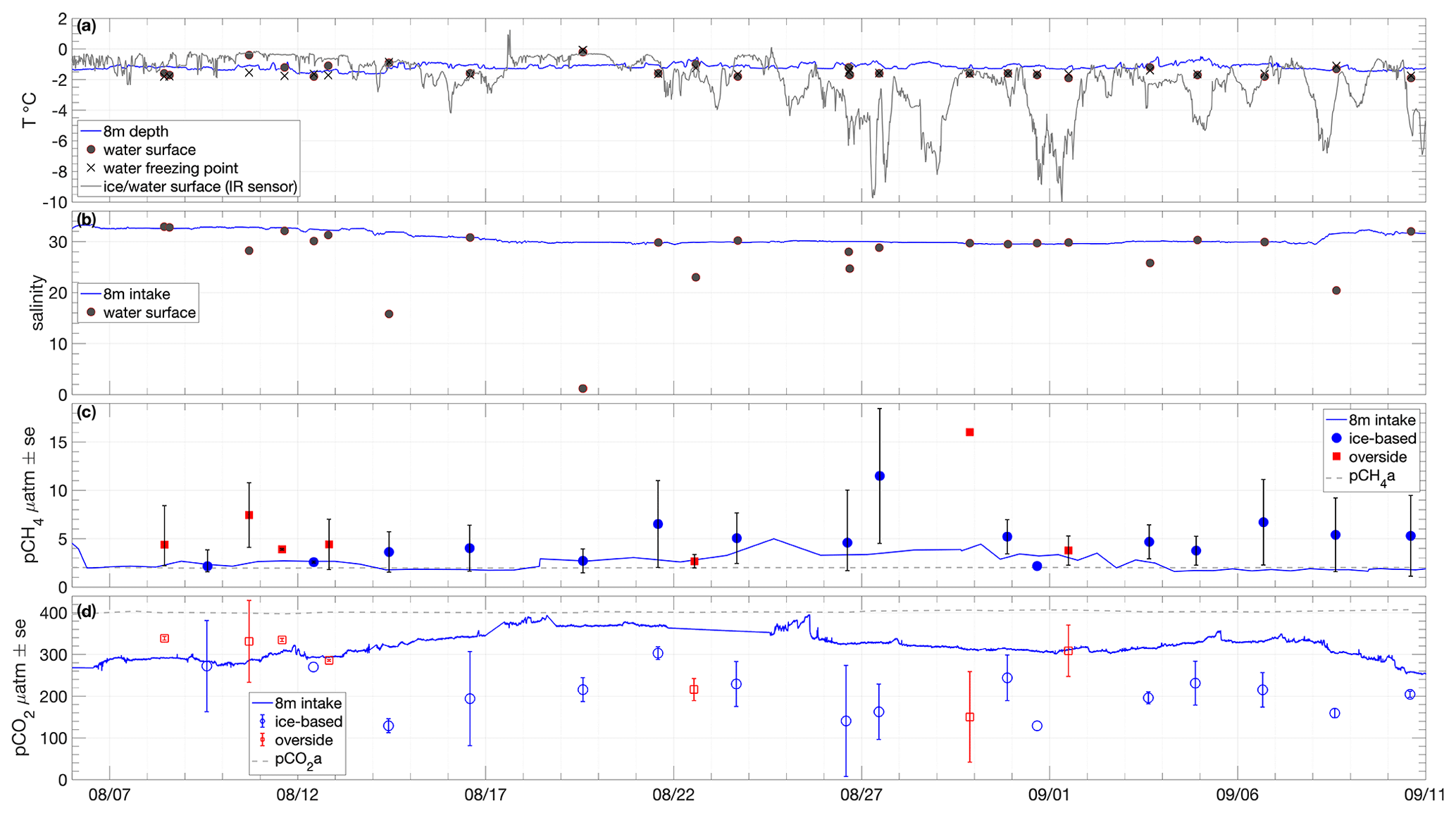
Figure 4Time series of (a) seawater temperature at 8 m depth and at the surface during chamber flux sampling, with the corresponding freezing point determined from salinity measurement and surface temperature (ice or water) measured from IR sensors on board Oden. (b) Salinity measured from the 8 m intake and at the surface during chamber flux sampling. (c) Partial pressures of CH4 in water at specified depths and sampling locations and in the near-surface atmosphere. (d) As per (c) for CO2.
Surface water temperature in leads sampled during flux measurements was −1.4 ± 0.5 ∘C (Fig. 4a), and the salinity of those samples showed high variation, ranging from 1.2 to 32.9, with an average of 26.3 ± 8.5 (Fig. 4b). Surface water temperatures were generally at or very close to the seawater freezing point. Salinity lower than 22 occurred when ice movement caused a release of fresh melt pond water into leads, resulting in strong near-surface gradients. The temperature and salinity measured from the 8 m depth intake showed less variation: −1.2 ± 0.2 ∘C and 30.8 ± 1.2, respectively. Surface temperatures determined by infrared sensors, including both ice and water surfaces, were −2.0 ± 1.7 ∘C over the course of the expedition. Approximately 20 % of the expedition occurred with surface temperatures below −3 ∘C and 30 % with surface temperatures above −1 ∘C (Fig. 3c).
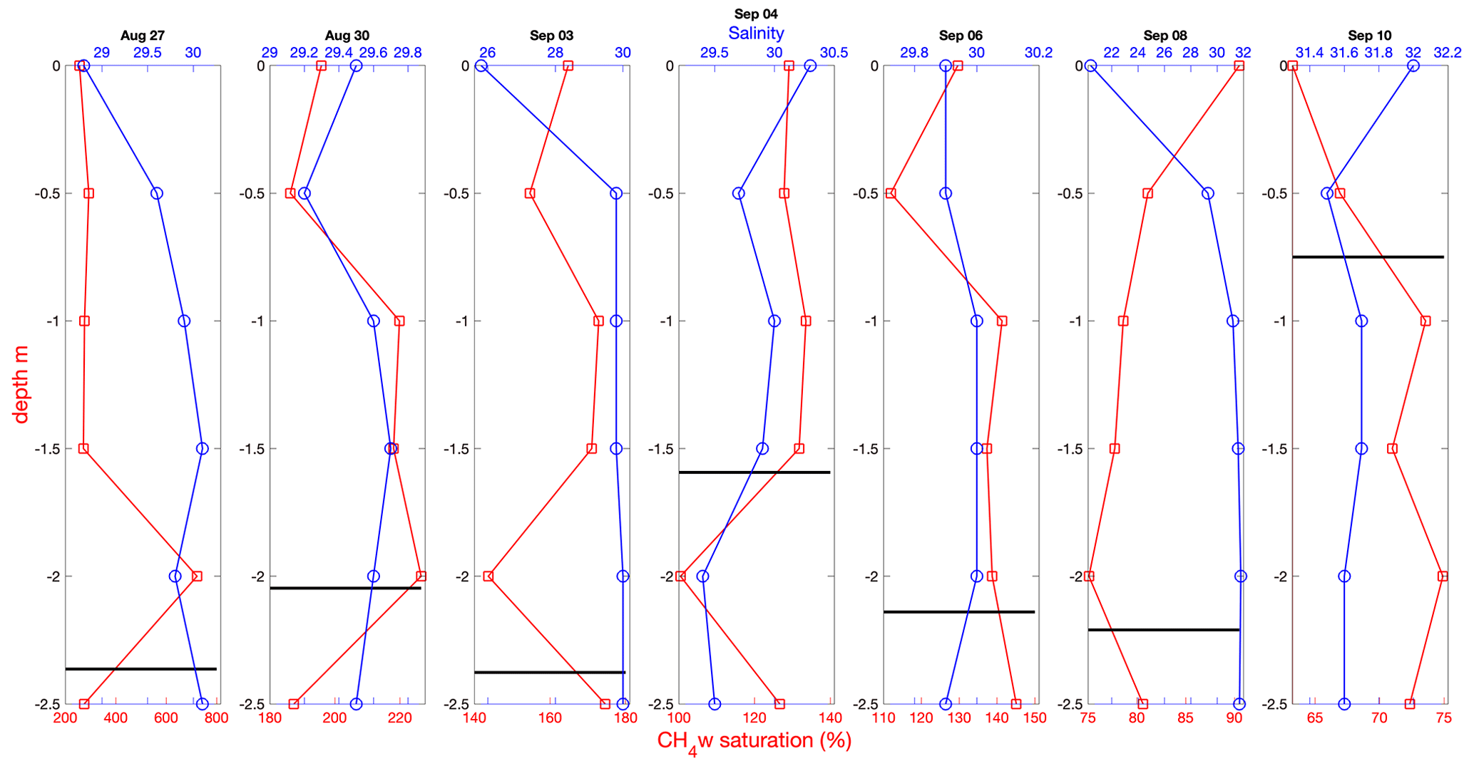
Figure 5Near-surface profiles of CH4 saturation (red) and salinity (blue) determined from ice-based Ruttner bottle sampling on the indicated day. An estimate of ice floe thickness is shown (thick black line), determined from auger drilling close to the sampling site.
Throughout the expedition, intermittent periods with falling surface temperatures occurred, associated with clear-sky conditions and surface longwave cooling (e.g. Prytherch and Yelland, 2021). From 25 August there was a regime shift, with protracted periods of surface (ice) temperature below the seawater freezing point and deeper intermittent surface temperature drops, falling to around −10 ∘C, indicating the beginning of the autumn freeze-up (Supplement Sect. S2 and Fig. S3 in the Supplement).
3.2 CH4 and CO2 partial pressures
Atmospheric CH4 partial pressure (pCH4a) measured using the chamber LGR analyser during equilibration periods, increased from approximately 1.98 µatm to 2.01 µatm over the course of the expedition (mean and standard deviation 1.99 ± 0.02 µatm; Fig. 4c). The surface seawater pCH4w was determined as the average of two GC-based sampling methods (Sect. 2.2), with the two methods having a mean standard error of 2.82 ± 1.54 µatm, with the syringe-based samples consistently higher (Supplement Sect. S1; Fig. S2a). The averaged surface seawater pCH4w measurements were slightly oversaturated throughout the expedition: 5.37 ± 3.13 µatm (Fig. 4c and Table S1). Overside samples were slightly higher and more variable (5.88 ± 4.32 µatm) than ice-based samples (5.05 ± 2.26 µatm), with the highest overside sample on 29 August at 16.0 µatm. The pCH4w sampled from 8 m depth was lower and less variable than the surface measurements, with an average of 2.70 ± 0.68 µatm. The 8 m pCH4w was closer to equilibrium than the surface waters but still slightly oversaturated, most notably from 18 August to 4 September, when pCH4w averaged 3.1 ± 0.8 µatm.
Near-surface gradients of CH4 saturation determined from Ruttner bottle sampling and on-ship analysis during the latter part of the expedition showed little variation with depth over the upper 2.5 m (Fig. 5). A pronounced freshening of the near-surface water was observed on 3 and 8 September and to a lesser extent on 27 August. This is likely to be either a residual layer from ice melt or due to leakage of fresh melt pond water resulting from ice movement caused by Oden's nearby passing.
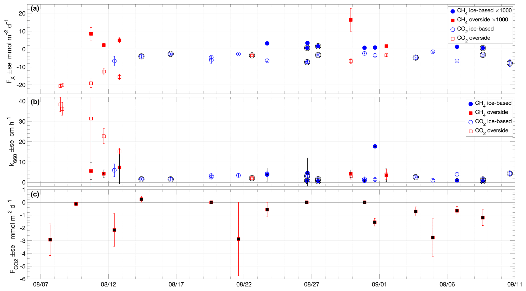
Figure 6Time series of (a) air–sea fluxes of CH4 (filled symbols) and CO2 (non-filled symbols) measured with chamber flux systems at the specified sampling locations; (b) k660 of CH4 (filled symbols) and CO2 (non-filled symbols) determined from air–sea chamber flux measurements using Eqs. (1) and (2); (c) snow–air CO2 fluxes measured with the EGM-4 chamber flux system. Error bars are the standard error of the flux samples in each deployment. Outer black circles in (a) and (b) indicate measurements made in the presence of grease ice.
Atmospheric CO2 partial pressure (pCO2a) from chamber equilibration periods was 402.4 ± 3.0 µatm (Fig. 4d). The surface seawater pCO2w was determined as the average of GC-based syringe samples and bottle samples analysed for DIC and TA from which pCO2 was calculated (Sect. 2.2). The two methods had a mean standard error of 25.5 ± 22 µatm (Supplement Sect. S1; Fig. S2b). The resulting averaged surface seawater pCO2w was always undersaturated, with a mean value of 227 ± 71 µatm (Fig. 4d and Table S1). The pCO2w from overside samples was higher and more variable (288 ± 69 µatm) than that from the ice-based samples (189 ± 39 µatm). The seawater pCO2w from 8 m depth was closer to equilibrium but still strongly undersaturated during most of the expedition: on average 315 ± 28 µatm. There was a strong gradient in pCO2w between the surface measurements and those from the 8 m intake from 14 August to the end of the expedition (Fig. 4d). Both depths were undersaturated throughout the expedition with the surface pCO2w on average 88 µatm lower than at 8 m depth. The period prior to 13 August had noticeably higher surface water pCO2w than later periods: close to or above the 8 m depth pCO2w. The surface measurements in this early period were from both overside and ice-based sampling, suggesting this relatively reduced or reversed pCO2w gradient was not primarily an artefact of Oden's influence on the upper water column.
3.3 Lead air–sea fluxes
All measured air–sea CH4 fluxes were positive (emission from the water to the atmosphere), in the direction of the air–sea concentration gradient, and the majority of the fluxes were less than 5 (Fig. 6a and Table S1). The two highest fluxes, on 11 and 29 August, were coincident with the strongest air–sea pCH4 differences (Fig. 4c). The average air–sea CH4 flux was 3.5 ± 4.4 . The overside flux measurements were on average higher and more variable (6.7 ± 6.0 ) than the ice-based measurements (1.5 ± 1.1 ).
Measured air–sea CO2 fluxes, using both the LGR- and Li-COR 7200-based systems, were all negative, showing uptake of CO2 by seawater. The flux was in the direction of the air–sea concentration gradient, with a range of −1.5 to −20.7 (Fig. 6a and Table S1). The average air–sea CO2 flux was −7.3 ± 5.7 . As for the CH4 fluxes, the average magnitude of the overside CO2 flux measurements was higher and more variable (−12.7 ± 7.3 ) than the ice-based measurements (−4.8 ± 2.0 ).
The largest CO2 fluxes occurred in the early part of the expedition, prior to 13 August, during overside sampling and in a period with a notably smaller air–sea pCO2 gradient than later. The large overside flux measurements on 8 August occurred during high winds, but other high overside measurements on 10 and 11 August occurred during light winds < 4 m s−1 (Fig. 2b). These measurements may be biased by the presence of Oden or the interaction between Oden and the floating chamber, affecting the near-surface turbulence that drives the flux. These biases likely depend on the interaction of conditions such as the wind speed and direction relative to Oden, the location and topology of sea ice, and the position of the chamber relative to Oden and to the sea ice, all of which varied from one sampling to another. As such, all overside flux measurements are treated separately to the ice-based measurements.
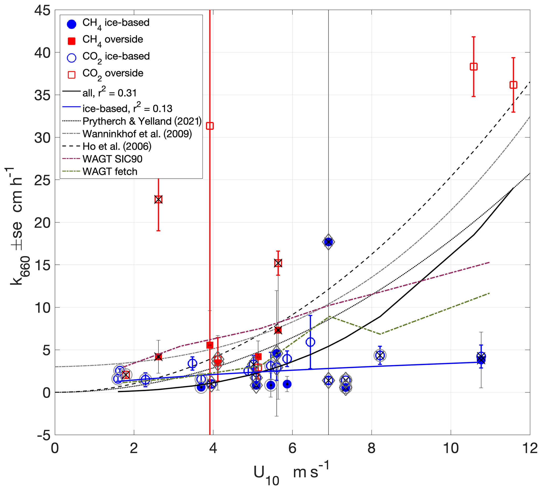
Figure 7Wind speed dependence of k660 determined from air–sea chamber flux measurements using Eqs. (1) and (2) and non-linear least-squares fits to the measurements (). Outer circles around the markers indicate measurements made in the presence of grease ice. Black crosses indicate measurements made with lead widths < 10 m. Diamonds indicate measurements made when the surface buoyancy flux was negative (surface cooling). Also shown are three wind-speed-based parameterisations of k660 and the parametric WAGT model in both SIC mode (with SIC = 90 %) and fetch mode using lead width.
Thin, grease or frazil ice was present at times during the expedition, especially during the latter part of the expedition, from 26 August, coinciding with the end of the melt season and the onset of the freeze-up. Ice-based sampling when grease ice was present resulted in lower fluxes on average of CH4 (0.9 ± 0.6 ), indicating that grease ice may impede gas exchange, presumably through the ice layer presenting both a physical barrier and reducing the action of wind on the surface water. However, the presence of grease ice did not change the average flux of CO2, and the mean reduction in CH4 flux is within the standard deviation. The presence of the chamber may modify the effect of the grease ice on gas exchange in an unquantified way, trapping ice inside or outside the chamber and modifying the radiative balance at the surface, affecting ice formation.
3.4 Gas transfer velocities
Gas transfer velocities (k660) determined directly from air–sea chamber flux measurements using Eqs. (1) and (2) were generally less than 10 cm h−1, with the notable exception of k660 determined from overside CO2 flux measurements prior to 13 August when winds and fluxes were high (Fig. 6b). For all measurements, the average k660 was 6.7 ± 9.7 cm h−1 (median 3.3 cm h−1). The average CH4-flux-derived k660 was 4.2 ± 4.6 cm h−1, while the average CO2-flux-derived k660 was 8.0 ± 11.4 cm h−1. The distribution of k660 is non-Gaussian, and the median values from both gases combined and for CH4 and CO2 separately are similar: 3.3, 3.8 and 3.1 cm h−1, respectively. The ice-based measurements were lower and had less scatter; the median k660 of both gases was 2.5 cm h−1 (average 3.0 ± 3.4 cm h−1). Many of the lower k660 measurements were made in the presence of grease or frazil ice, with the median k660 of grease ice affected, ice-based samples of both gases being 1.1 cm h−1 (average 1.4 ± 0.9 cm h−1).
The wind speed dependence of the measurements, determined with a non-linear least-squares fit of the form , was approximately cubic, although the correlation with the data was weak (a = 0.02, b = 2.9, r2 = 0.31; Fig. 7). The two measurements with the greatest uncertainty (standard errors of 289 and 45 cm h−1) were excluded from the fit. The relatively few data points (36) and the weakness of the correlation means that caution is needed in interpretation or application of this relationship. At low wind speeds (< 3 m s−1), the measurements are higher than previously determined power law parameterisations, suggesting that processes other than wind speed may be contributing to interfacial mixing. With the exception of one value, these low wind k660 are relatively small, similar to the low-wind values of previous parameterisations determined with non-zero intercepts (e.g. Wanninkhof et al., 2009).
The overside CO2-flux-derived k660 was higher and more scattered than the other measurements and may have been affected by their close proximity to Oden's hull and the additional turbulence that this may induce in the ocean. The wind speed dependence of the fit determined to only ice-based measurements (again excluding the measurement with the highest standard error) was weaker and had a weaker correlation (a = 0.999, b = 0.533, r2 = 0.13). The ice-based measurements would not have been affected by any such bias, and the wind speed dependence of ice-based CO2- and CH4-derived k660 was weaker, close to linear and generally below previous open ocean and lead water k660 parameterisations. The contribution to the observed k660 wind speed dependence of forcings particular to the sea-ice environment is discussed in Sect. 4.2.
The measurements were also compared with the parametric Wave Age Gas Transfer (WAGT) model of gas exchange in sea-ice regions (Bigdeli et al., 2018). The WAGT model was run in both SIC mode, with SIC set to 90 %, and fetch mode using the lead width measurements. The WAGT fetch mode has good agreement with the measurements at wind speeds below 6 m s−1, whereas the SIC mode overpredicts. Both WAGT modes overpredict at higher wind speeds.
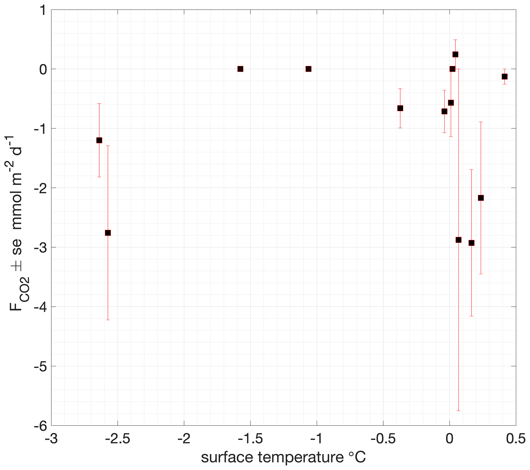
Figure 8Surface temperature dependence of ice–air and snow–air CO2 fluxes measured with the EGM-4 chamber flux system.
3.5 Air–snow fluxes
Chamber measurements of air–snow CO2 flux showed consistent small fluxes (on average, −1.1 ± 1.2 ), with the largest-magnitude flux −2.9 (Fig. 6c and Table S2). No clear dependence of the atmospheric flux on surface temperature was found, with the largest-magnitude fluxes occurring at temperatures close to and above freezing but some relatively large fluxes (up to −2.8 ) also being observed during the coldest measured surface conditions, with temperatures < −2 ∘C (Fig. 8).
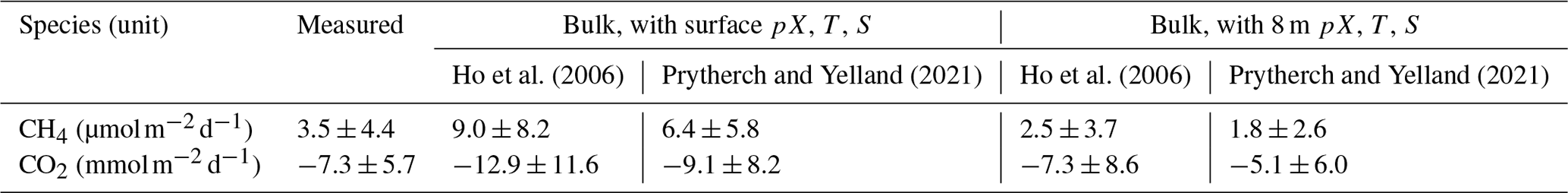
Table 1Air–sea CH4 and CO2 fluxes (mean ± standard deviation) determined from chamber measurements and from bulk methods using the specified gas transfer relationship and partial pressure, temperature and salinity measurement location.
4.1 Near-surface concentration gradients
Strong near-surface CO2 gradients are often observed in Arctic waters. Lower CO2 partial pressure at the surface relative to 8 m (Fig. 4d) may result from the input of unsaturated water from melting sea ice, from differences in biological activity and from the increased solubility resulting from the generally lower temperature and fresher surface waters (Fig. 4a and b). Solubility differences between the surface and 8 m in the measurements reported here on average account for a pCO2w difference of 10 µatm or 11 % of the total average difference between the depths. The fresher surface layer observed on several days (27 August, 3 and 8 September; Fig. 5) indicates a stratification that could act to suppress near-surface mixing, leading to lower surface gas concentrations and thus lower fluxes. In the coarse vertical-resolution observations reported here, near-surface CH4 saturations decrease in the presence of lower salinity, suggesting that in these cases the greater solubility in fresher water compensates for any stratification effect.
The results here further demonstrate the concentration gradients that can be present between the surface and the sampling depths used for the majority of the reported ocean “surface” gas concentration measurement (e.g. Miller et al., 2019). Larger air–sea concentration differences will, all else being equal, cause a larger air–sea flux, and thus any gradient between the surface and the water sampling depth will bias both bulk-method fluxes (i.e. fluxes calculated using Eq. 1 and a parameterisation of k; Wanninkhof et al., 2009) and gas transfer velocity measurements. As such gradients are common and are not easy to determine or correct for, many parameterisations of gas transfer incorporate such biases.
If the surface partial pressure, T and S measurements from this study are used to determine bulk-method fluxes, the CO2 fluxes are on average 77 % (with the k−U10 relationship of Ho et al., 2006) or 25 % (with the k−U10 relationship of Prytherch and Yelland, 2021) higher than the measured chamber fluxes (Table 1). This result adds to the existing literature showing a physical effect of sea ice on gas transfer velocity. In contrast, if the 8 m depth partial pressure, T and S measurements are used instead, the bulk fluxes are 1 % (Ho et al., 2006) and 30 % lower (Prytherch and Yelland, 2021) than the measured fluxes. This result adds to those discussing the bias in bulk fluxes, particularly prevalent in the Arctic, when gas concentration measurements are made at depth below the air–water interface (e.g. Miller et al., 2019). For CH4 the effects of the gradients are similar (Table 1), with bulk fluxes derived from surface measurements being larger than the chamber fluxes by 156 % and 80 % (for the Ho et al., 2006, and Prytherch and Yelland, 2021, k−U10 relationships, respectively) and the bulk fluxes derived from 8 m measurements being smaller than the chamber flux measurements by 28 % and 49 %, respectively.
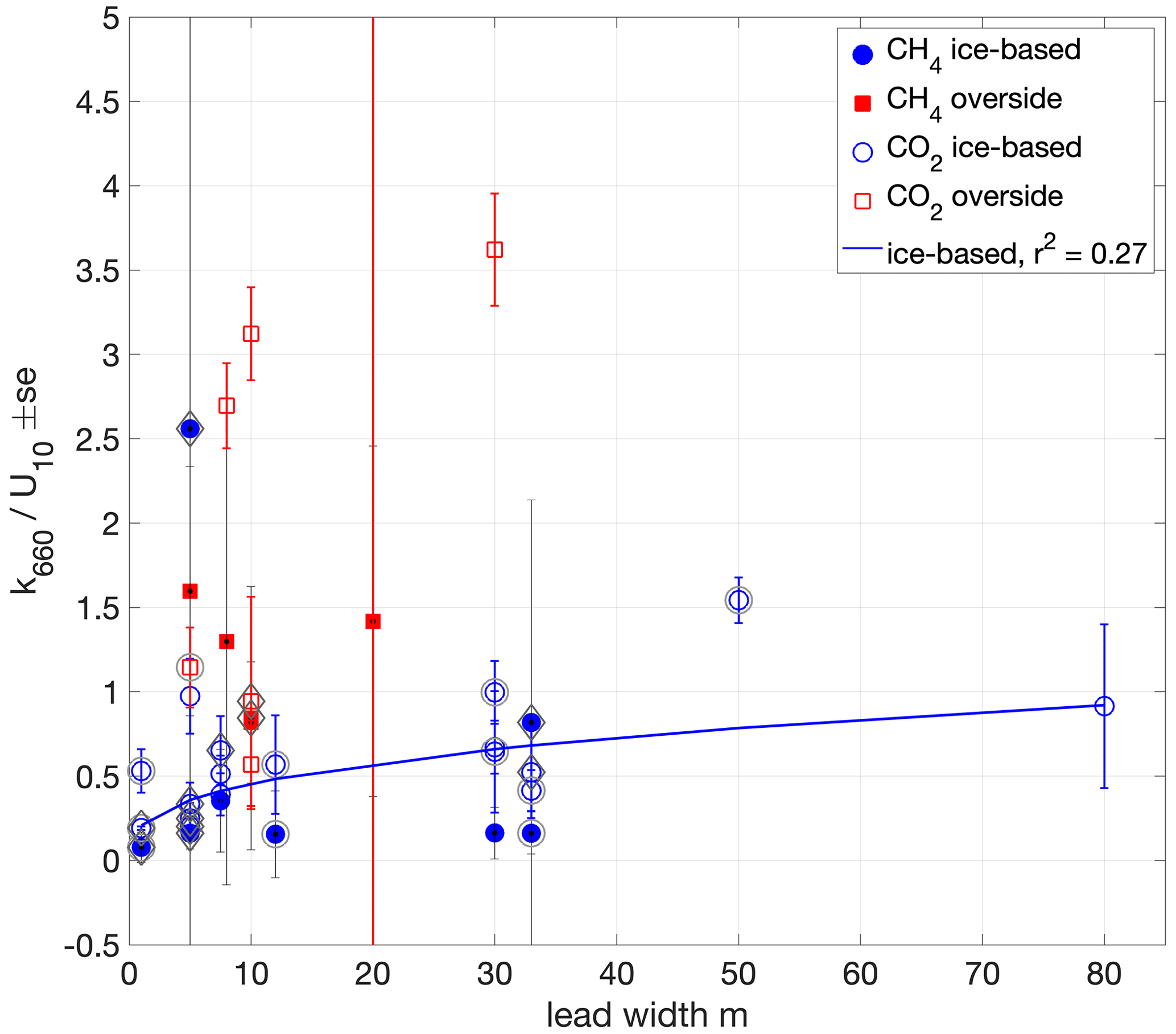
Figure 9Dependence on lead width of water–air chamber flux-derived k660 normalised by U10. A non-linear least-squares fit to the ice-based measurements () is shown (blue line). Outer circles around the markers indicate measurements made in the presence of grease ice. Diamonds indicate measurements made when the surface buoyancy flux was negative (surface cooling).
4.2 Gas transfer in the presence of sea ice
Greater lead width and fetch enables greater wind-driven mixing, while measurements close to ice edges may also be affected by the interaction of wind and waves with the ice edge. The wind speed dependence of all (36) measurements (Fig. 7) is approximately cubic with a weak correlation (r2 0.31). The k660 measurements, normalised by U10, do not show a clear dependence on lead width as determined by laser ranging (Fig. 9). For overside measurements lead width was the distance from Oden's hull to the ice edge. In contrast, the U10-normalised ice-based measurements appear to have a dependence on lead width; the correlation of a non-linear least-squares fit of the form is weak (a = 0.208, b = 0.34, r2 = 0.27) but stronger than the fit of these measurements to wind speed. Properly accounting for such fetch effects would require the determination of lead dimensions, relative wind direction and ice freeboard, but the relatively small variation in the ice-based measurements with width suggests that simpler approaches to parameterising k in sea-ice regions, with either a wind speed dependence or a constant value, may be sufficient.
The buoyancy flux measurements enable the identification of measurements made in conditions of surface-cooling-induced convection, which can enhance gas exchange (McGillis et al., 2004), but no clear enhancement of gas transfer was apparent (Fig. 7). Many of the convective measurements were also in leads of < 10 m width (Figs. 7 and 9), complicating the determination of the impact of either convection or fetch on gas exchange. Many, but not all, of the lower gas exchange rates were measured when grease ice was present on the lead water, even at higher wind speeds (> 7 m s−1) when low lead widths provided sheltered conditions (Fig. 7). Grease ice is expected to reduce gas transfer rates, and all high k660 measurements (> 5 cm h−1), both overside and ice-based, were obtained when grease ice was not present.
The WAGT model was designed to use estimates of the area of open water from SIC products. Although different ice products have experienced significant improvements in increased resolution in recent years, they are still prone to missing critical small-scale features such as open or refrozen leads. Passive radiometer data also treat a ∼ 20 cm thin ice cover as open water (e.g. Hoffman et al., 2019), with severe impacts on gas transfer estimates.
4.3 Regional fluxes
The fluxes and gas transfer measurements presented here provide direct-measurement-based constraints for the role of the CAO in CO2 and CH4 atmospheric exchange. Air–sea chamber fluxes were made at latitudes from approximately 82.5 to 90∘ N. These latitudes bound an area of 2.2 × 10⁶ km2, approximately corresponding to the deep-water areas of the Amundsen Basin. The International Hydrographic Organization (IHO)-defined central Arctic deep basin (4.7 × 10⁶ km2) and the bathymetrically defined 4.5 × 10⁶ km2 “Central Arctic Ocean Basin” delineated by Jakobsson (2002) and used here as the definition of the CAO are larger. In all definitions, the CAO corresponds to the Arctic Ocean deep water > 2400 m depth, as a strong contrast to the shallow shelf seas (average depths ∼ 50–250 m) which surround the Arctic Ocean. The average SIC during this portion of the expedition was 90 %, determined from AMSR-2 6.25 km2 observations using the ASI algorithm (Spreen et al., 2008).
The measured air–sea CO2 fluxes are of similar magnitude to the EC measurements of Prytherch et al. (2017) (average −7.8 ), Prytherch and Yelland (2021) (0 to −20 , average −12.4 , measured in higher winds) and Dong et al. (2021), (0 to −40 , measured in SIC > 60 %). Averaging observations regionally, the mean chamber-derived CO2 air–sea fluxes of −7.6 correspond to SIC-accounted CAO fluxes of −3.42 × 10⁹ mol d−1 or −150.5 Gg CO2 d−1. The flux measurements reported here were made during the summer and the beginning of the autumn freeze-up in conditions of persistent, strong pCO2w undersaturation. The annual cycle of Arctic Ocean surface pCO2w is poorly constrained, primarily due to the rarity of reported observations outside of summer months (e.g. Yasunaka et al., 2018; Else et al., 2012). As such, while we can estimate an annual CAO air–sea flux of −55.0 Tg CO2 yr−1 by multiplying the average daily flux by 365, this result is highly uncertain. Furthermore, while density stratification from sea-ice melt in summer months may suppress upper-ocean mixing leading to reduced air–sea concentration gradients and thus reduced summer fluxes relative to other seasons, this stratification was not evident in the measurements reported here. Thus, due to the higher SIC and lower primary productivity in winter months, our annual flux estimate is likely to represent a high estimate. If the average bulk flux of −8.4 as determined from near-surface CO2 concentrations and the k relationship of Prytherch and Yelland (2021) is used instead of the average observed flux, the CAO air–sea flux is slightly larger (−3.78 × 10⁹ mol d−1 or −166.4 Gg CO2 d−1).
The measured air–snow CO2 fluxes (−1.1 ± 1.2 ) are of a similar magnitude to previously reported EC-determined air–snow fluxes from the summertime CAO (Prytherch and Yelland, 2021; −0.7 , maximum −6.5 ). They also span a similar range (−2.9 to 0.25 ) including the observed positive emission fluxes, as previously reported air–snow chamber flux measurements (Geilfus et al., 2012; Nomura et al., 2010, 2013, 2018; Delille et al., 2014; Geilfus et al., 2015). However, none of these previously reported air–snow flux measurements are from the summertime or autumn CAO. Using the observed expedition SIC and the average flux through snow-covered sea ice of −1.1 yields a CAO regional air–snow flux of −4.46 × 10⁹ mol d−1 or −196.1 Gg d−1. Combining the air–sea and air–snow chamber flux estimates with constant SIC (90 %), the average atmospheric CO2 flux for the CAO is −1.75 .
The average air–sea CH4 flux of 3.5 , accounting for SIC, equates to a CAO flux of 1.58 × 10⁶ mol d−1 or 25.3 Mg d−1. Similarly, the average bulk CH4 flux of 5 derived from near-surface CH4 concentrations and the k relationship of Prytherch and Yelland (2021) corresponds to 36.1 Mg d−1 for the CAO area. The annual cycle of Arctic Ocean surface CH4 is much less well known than for CO2, in particular the origin of the dissolved CH4 driving the observed fluxes. As such the extrapolation of our observations and bulk estimates to annual fluxes (9.2 and 13.2 Gg yr−1, respectively) is also highly uncertain. Both the directly observed and bulk-flux-derived annual estimates are likely to be high estimates due to the higher SIC and minimal release of CH4 from within sea ice during winter.
Stratification of near-surface waters by freshening from meltwater may reduce air–sea gas flux by both reducing the turbulent mixing below the interfacial layer, dampening the gas transfer velocity, and by impeding the replenishment of the equilibrating surface waters from the bulk water below, reducing the concentration difference that drives the exchange. Suppression of turbulent mixing may contribute to the observed difference between chamber and bulk fluxes; however, the surface layer freshwater stratification apparent in surface layers did not coincide with CH4 stratification (Fig. 5).
Both the direct chamber CH4 fluxes and bulk CH4 fluxes are of similar magnitude to previously reported flux estimates derived from seawater CH4 measurements in summer and winter at more southerly Arctic marine locations (e.g. Lorenson et al., 2016; Manning et al., 2020, 2022; Fenwick et al., 2017; Silyakova et al., 2022) but are approximately 35 times smaller than aircraft-based observations of fluxes from wintertime leads over the western CAO's Canada Basin, south of 82∘ N (Kort et al., 2012). This suggests a strong seasonal dependence of CAO CH4 flux or that the aircraft-based measurements of large fluxes represent episodic rather than typical widespread emissions or erroneous measurements. If we assume that the fluxes reported by Kort et al. (2012) are more typical of the Canada Basin and distinct from our primarily Amundsen Basin study area, this suggests a much higher net annual CH4 flux from the CAO of up to ∼ 0.1 Tg yr−1. The CAO has a mean depth > 2700 m (Jakobsson, 2002), meaning any CH4 emissions must be from near-surface production or long-range transport of dissolved CH4; seafloor sources are too deep to significantly affect the surface pCH4w in the CAO.
The direct flux and gas transfer measurements presented in this study offer insights into the role of the CAO in atmospheric exchange of climate forcing trace gases, informing future climate modelling and carbon budget analysis. They provide a measurement-based constraint on the magnitude of the CAO CO2 flux, with the observed CAO CO2 flux in agreement with the observation-based estimates of Bates et al. (2006) and Yasunaka et al. (2018) and an order of magnitude greater than the coupled ocean–biogeochemistry model estimate of Manizza et al. (2019). For CH4, the direct-measurement-based constraints determined here show that the CAO is a very small additional contributor to the Arctic Ocean CH4 flux in summer, with the mean CAO CH4 flux of 25.3 Mg d−1 comprising approximately 0.002 of the estimate of integrated Arctic marine CH4 emissions of 4–5 Tg yr−1 (Thornton et al., 2016a, b, 2020) if that estimate is assumed to be evenly distributed over the year. Arctic marine CH4 emissions are dominated by the shallow coastal shelf emissions.
While the observed gas transfer velocities had a similar, if weakly correlated, wind speed dependence to that of Prytherch and Yelland (2021), the wind speed dependence of the ice-based measurements, free from any influence of Oden on the exchange rate, was much weaker. The measurements reported here, from pack ice regions with small water surfaces, could be appropriately represented with a constant k660 of 2.5 cm h−1 instead of a relationship directly or indirectly (i.e. wave- or turbulence-based) dependent on wind speed. In areas such as the marginal ice zone with mixed sea ice and water and larger fetches, the direct and indirect influence of wind on interfacial mixing will be greater and gas exchange should be represented using a parameterisation incorporating wind speed such as Prytherch and Yelland (2021).
The raw and processed data and the underlying code for the data and analysis presented in this manuscript are published at https://doi.org/10.6084/m9.figshare.25109177 (Prytherch, 2024).
The supplement related to this article is available online at: https://doi.org/10.5194/bg-21-671-2024-supplement.
JP designed the experiment, JP and SM carried out the flux measurements and water sampling, and JP, IB, VB, AU, ALH, ATN and LAH analysed the water samples. JP, BFT and MT developed the ship-based instrumentation, and JP and VB developed the chamber flux systems. JP prepared the paper with contributions from all co-authors.
The contact author has declared that none of the authors has any competing interests.
Publisher's note: Copernicus Publications remains neutral with regard to jurisdictional claims made in the text, published maps, institutional affiliations, or any other geographical representation in this paper. While Copernicus Publications makes every effort to include appropriate place names, the final responsibility lies with the authors.
The Swedish Polar Research Secretariat (SPRS) provided access to the icebreaker (I/B) Oden and logistical support. We would like to thank Capt. Mattias Petersson and the crew of Oden for their invaluable support throughout the field campaign. Thanks also to the Chief Scientist Pauline Snoeijs Leijonmalm for the planning and coordination of SAS2021.
John Prytherch and Sonja Murto were supported by the Knut and Alice Wallenberg Foundation (grant no. 2016-0024). Adam Ulfsbo was supported by the Swedish Research Council Formas (grant no. 2018-01398) and the Hasselblad Foundation (grant no. 2019-1218). Lina A. Holthusen was supported by the Arctic Research Icebreaker Consortium (ARICE, EU, https://arice-h2020.eu, last access: 30 January 2024) (grant no. 730 965). This paper contributes to the science plan of the Surface Ocean-Lower Atmosphere Study (SOLAS), which is partially supported by the U.S. National Science Foundation (grant no. OCE-1840868) via the Scientific Committee on Oceanic Research (SCOR).
The article processing charges for this open-access publication were covered by Stockholm University.
This paper was edited by Manmohan Sarin and reviewed by Brent G. T. Else, Richard Sims, and one anonymous referee.
Ahmed, M. M. M., Else, B. G. T., Capelle, D., Miller, L. A., and Papakyriakou, T.: Underestimation of surface pCO2 and air–sea CO2 fluxes due to freshwater stratification in an Arctic shelf sea, Hudson Bay, Elementa: Science of the Anthropocene, 8, 084, https://doi.org/10.1525/elementa.084, 2020.
Bastviken, D., Ejlertsson, J., Sundh, I., and Tranvik, L.: METHANE AS A SOURCE OF CARBON AND ENERGY FOR LAKE PELAGIC FOOD WEBS, Ecology, 84, 969–981, https://doi.org/10.1890/0012-9658(2003)084[0969:maasoc]2.0.co;2, 2003.
Bates, N. R. and Mathis, J. T.: The Arctic Ocean marine carbon cycle: evaluation of air-sea CO2 exchanges, ocean acidification impacts and potential feedbacks, Biogeosciences, 6, 2433–2459, https://doi.org/10.5194/bg-6-2433-2009, 2009.
Bates, N. R., Moran, S. B., Hansell, D. A., and Mathis, J. T.: An increasing CO2 sink in the Arctic Ocean due to sea-ice loss, Geophys. Res. Lett., 33, L23609, https://doi.org/10.1029/2006gl027028, 2006.
Bigdeli, A., Hara, T., Loose, B., and Nguyen, A. T.: Wave Attenuation and Gas Exchange Velocity in Marginal Sea Ice Zone, J. Geophys. Res.-Oceans, 123, 2293–2304, https://doi.org/10.1002/2017jc013380, 2018.
Butterworth, B. J. and Miller, S. D.: Air–sea exchange of carbon dioxide in the Southern Ocean and Antarctic marginal ice zone, Geophys. Res. Lett., 43, 7223–7230, https://doi.org/10.1002/2016gl069581, 2016.
Cole, J. J., Bade, D. L., Bastviken, D., Pace, M. L., and Van de Bogert, M.: Multiple approaches to estimating air–water gas exchange in small lakes, Limnol. Oceanogr.-Meth., 8, 285–293, https://doi.org/10.4319/lom.2010.8.285, 2010.
Damm, E., Rudels, B., Schauer, U., Mau, S., and Dieckmann, G.: Methane excess in Arctic surface water- triggered by sea ice formation and melting, Sci. Rep.-UK, 5, 16179, https://doi.org/10.1038/srep16179, 2015.
Damm, E., Bauch, D., Krumpen, T., Rabe, B., Korhonen, M., Vinogradova, E., and Uhlig, C.: The Transpolar Drift conveys methane from the Siberian Shelf to the central Arctic Ocean, Sci. Rep.-UK, 8, 4515, https://doi.org/10.1038/s41598-018-22801-z, 2018.
Delille, B., Vancoppenolle, M., Geilfus, N.-X., Tilbrook, B., Lannuzel, D., Schoemann, V., Becquevort, S., Carnat, G., Delille, D., Lancelot, C., Chou, L., Dieckmann, G. S., and Tison, J.-L.: Southern Ocean CO2 sink: The contribution of the sea ice, J. Geophys. Res.-Oceans, 119, 6340–6355, https://doi.org/10.1002/2014jc009941, 2014.
Dickson, A. G., Sabine, C. L. and Christian, J. R. (Eds.): Guide to Best Practices for Ocean CO2 Measurements, PICES Special Publication 3, 191 pp. 2007.
Dong, Y., Yang, M., Bakker, D. C. E., Liss, P. S., Kitidis, V., Brown, I., Chierici, M., Fransson, A., and Bell, T. G.: Near-Surface Stratification Due to Ice Melt Biases Arctic Air–Sea CO2 Flux Estimates, Geophys. Res. Lett., 48, e2021GL095266, https://doi.org/10.1029/2021gl095266, 2021.
Else, B. G. T., Papakyriakou, T. N., Galley, R. J., Mucci, A., Gosselin, M., Miller, L. A., Shadwick, E. H., and Thomas, H.: Annual cycles of pCO2sw in the southeastern Beaufort Sea: New understandings of air–sea CO2 exchange in arctic polynya regions, J. Geophys. Res., 117, , C00G13, https://doi.org/10.1029/2011jc007346, 2012.
Fairall, C. W., Yang, M., Brumer, S. E., Blomquist, B. W., Edson, J. B., Zappa, C. J., Bariteau, L., Pezoa, S., Bell, T. G., and Saltzman, E. S.: Air–Sea Trace Gas Fluxes: Direct and Indirect Measurements, Front. Mar. Sci., 9, 826606, https://doi.org/10.3389/fmars.2022.826606, 2022.
Fanning, K. A. and Torres, L. M.: 222Rn and 226Ra: indicators of sea-ice effects on air–sea gas exchange, Polar Res., 10, 51–58, https://doi.org/10.3402/polar.v10i1.6727, 1991.
Fenwick, L., Capelle, D., Damm, E., Zimmermann, S., Williams, W. J., Vagle, S., and Tortell, P. D.: Methane and nitrous oxide distributions across the North American Arctic Ocean during summer, 2015, J. Geophys. Res.-Oceans, 122, 390–412, https://doi.org/10.1002/2016jc012493, 2017.
Fransson, A., Chierici, M., Skjelvan, I., Olsen, A., Assmy, P., Peterson, A. K., Spreen, G., and Ward, B.: Effects of sea-ice and biogeochemical processes and storms on under-ice water f CO2 during the winter-spring transition in the high AO: Implications for sea-air CO2 fluxes, J. Geophys. Res.-Oceans, 122, 5566–5587, https://doi.org/10.1002/2016jc012478, 2017.
Gålfalk, M., Bastviken, D., Fredriksson, S., and Arneborg, L.: Determination of the piston velocity for water–air interfaces using flux chambers, acoustic Doppler velocimetry, and IR imaging of the water surface, J. Geophys. Res.-Biogeo., 118, 770–782, https://doi.org/10.1002/jgrg.20064, 2013.
Geilfus, N.-X., Carnat, G., Papakyriakou, T., Tison, J.-L., Else, B., Thomas, H., Shadwick, E., and Delille, B.: Dynamics of pCO2 and related air–ice CO2 fluxes in the Arctic coastal zone (Amundsen Gulf, Beaufort Sea), J. Geophys. Res., 117, C00G10, https://doi.org/10.1029/2011jc007118, 2012.
Geilfus, N.-X., Galley, R. J., Crabeck, O., Papakyriakou, T., Landy, J., Tison, J.-L., and Rysgaard, S.: Inorganic carbon dynamics of melt-pond-covered first-year sea ice in the Canadian Arctic, Biogeosciences, 12, 2047–2061, https://doi.org/10.5194/bg-12-2047-2015, 2015.
Haraldsson, C., Anderson, L. G., Hassellöv, M., Hulth, S., and Olsson, K.: Rapid, high-precision potentiometric titration of alkalinity in ocean and sediment pore waters, Deep-Sea Res. Pt. I, 44, 2031–2044, https://doi.org/10.1016/s0967-0637(97)00088-5, 1997.
Ho, D. T., Law, C. S., Smith, M. J., Schlosser, P., Harvey, M., and Hill, P.: Measurements of air–sea gas exchange at high wind speeds in the Southern Ocean: Implications for global parameterizations, Geophys. Res. Lett., 33, L16611, https://doi.org/10.1029/2006gl026817, 2006.
Hoffman, J., Ackerman, S., Liu, Y., and Key, J.: The Detection and Characterization of Arctic Sea Ice Leads with Satellite Imagers, Remote Sens.-Basel, 11, 521, https://doi.org/10.3390/rs11050521, 2019.
Jähne, B., Münnich, K. O., Bösinger, R., Dutzi, A., Huber, W., and Libner, P.: On the parameters influencing air–water gas exchange, J. Geophys. Res., 92, 1937, https://doi.org/10.1029/jc092ic02p01937, 1987.
Jakobsson, M.: Hypsometry and volume of the Arctic Ocean and its constituent seas, Geochem. Geophy. Geosy., 3, 1–18, https://doi.org/10.1029/2001gc000302, 2002.
Johnson, K. M., Sieburth, J. M., leB Williams, P. J., and Brändström, L.: Coulometric total carbon dioxide analysis for marine studies: Automation and calibration, Mar. Chem., 21, 117–133, https://doi.org/10.1016/0304-4203(87)90033-8, 1987.
Kort, E. A., Wofsy, S. C., Daube, B. C., Diao, M., Elkins, J. W., Gao, R. S., Hintsa, E. J., Hurst, D. F., Jimenez, R., Moore, F. L., Spackman, J. R., and Zondlo, M. A.: Atmospheric observations of Arctic Ocean methane emissions up to 82∘ north, Nat. Geosci., 5, 318–321, https://doi.org/10.1038/ngeo1452, 2012.
Kwok, R.: Arctic sea ice thickness, volume, and multiyear ice coverage: losses and coupled variability (1958–2018), Environ. Res. Lett., 13, 105005, https://doi.org/10.1088/1748-9326/aae3ec, 2018.
Lewis, E. and Wallace, D. W. R.: Program Developed for CO2 System Calculations, ORNL/CDIAC-105, Carbon Dioxide Information Analysis Center, Oak Ridge National Laboratory, U.S. Department of Energy, Oak Ridge, Tennessee, 1998.
Loose, B., Schlosser, P., Perovich, D., Ringelberg, D., Ho, D. T., Takahashi, T., Richter-Menge, J., Reynolds, C. M., Mcgillis, W. R., and Tison, J.-L.: Gas diffusion through columnar laboratory sea ice: implications for mixed-layer ventilation of CO2 in the seasonal ice zone, Tellus B, 63, 23, https://doi.org/10.1111/j.1600-0889.2010.00506.x, 2011.
Loose, B., McGillis, W. R., Perovich, D., Zappa, C. J., and Schlosser, P.: A parameter model of gas exchange for the seasonal sea ice zone, Ocean Sci., 10, 17–28, https://doi.org/10.5194/os-10-17-2014, 2014.
Loose, B., Kelly, R. P., Bigdeli, A., Williams, W., Krishfield, R., Rutgers van der Loeff, M., and Moran, S. B.: How well does wind speed predict air–sea gas transfer in the sea ice zone? A synthesis of radon deficit profiles in the upper water column of Arctic Ocean, J. Geophys. Res.-Oceans, 122, 3696–3714, https://doi.org/10.1002/2016jc012460, 2017.
Lorenson, T. D., Greinert, J., and Coffin, R. B.: Dissolved methane in the Beaufort Sea and the Arctic Ocean, 1992–2009; sources and atmospheric flux, Limnol. Oceanogr., 61, S300–S323, https://doi.org/10.1002/lno.10457, 2016.
Lorke, A., Bodmer, P., Noss, C., Alshboul, Z., Koschorreck, M., Somlai-Haase, C., Bastviken, D., Flury, S., McGinnis, D. F., Maeck, A., Müller, D., and Premke, K.: Technical note: drifting versus anchored flux chambers for measuring greenhouse gas emissions from running waters, Biogeosciences, 12, 7013–7024, https://doi.org/10.5194/bg-12-7013-2015, 2015.
Lovely, A., Loose, B., Schlosser, P., McGillis, W., Zappa, C., Perovich, D., Brown, S., Morell, T., Hsueh, D., and Friedrich, R.: The Gas Transfer through Polar Sea ice experiment: Insights into the rates and pathways that determine geochemical fluxes, J. Geophys. Res.-Oceans, 120, 8177–8194, https://doi.org/10.1002/2014jc010607, 2015.
Lueker, T. J., Dickson, A. G., and Keeling, C. D.: Ocean pCO2 calculated from dissolved inorganic carbon, alkalinity, and equations for K1 and K2: validation based on laboratory measurements of CO2 in gas and seawater at equilibrium, Mar. Chem., 70, 105–119, https://doi.org/10.1016/s0304-4203(00)00022-0, 2000.
Lundevall-Zara, M., Lundevall-Zara, E., and Brüchert, V.: Sea-Air Exchange of Methane in Shallow Inshore Areas of the Baltic Sea, Front. Mar. Sci., 8, 657459, https://doi.org/10.3389/fmars.2021.657459, 2021.
MacIntyre, S., Fram, J. P., Kushner, P. J., Bettez, N. D., O'Brien, W. J., Hobbie, J. E., and Kling, G. W.: Climate-related variations in mixing dynamics in an Alaskan arctic lake, Limnol. Oceanogr., 54, 2401–2417, https://doi.org/10.4319/lo.2009.54.6_part_2.2401, 2009.
MacIntyre, S., Jonsson, A., Jansson, M., Aberg, J., Turney, D. E., and Miller, S. D.: Buoyancy flux, turbulence, and the gas transfer coefficient in a stratified lake, Geophys. Res. Lett., 37, L24604, https://doi.org/10.1029/2010gl044164, 2010.
Manizza, M., Menemenlis, D., Zhang, H., and Miller, C. E.: Modeling the Recent Changes in the Arctic Ocean CO2 Sink (2006–2013), Global Biogeochem. Cy., 33, 420–438, https://doi.org/10.1029/2018gb006070, 2019.
Mannich, M., Fernandes, C. V. S., and Bleninger, T. B.: Uncertainty analysis of gas flux measurements at air–water interface using floating chambers, Ecohydrology & Hydrobiology, 19, 475–486, https://doi.org/10.1016/j.ecohyd.2017.09.002, 2019.
Manning, C. C., Preston, V. L., Jones, S. F., Michel, A. P. M., Nicholson, D. P., Duke, P. J., Ahmed, M. M. M., Manganini, K., Else, B. G. T., and Tortell, P. D.: River Inflow Dominates Methane Emissions in an Arctic Coastal System, Geophys. Res. Lett., 47, e2020GL087669, https://doi.org/10.1029/2020gl087669, 2020.
Manning, C. C. M., Zheng, Z., Fenwick, L., McCulloch, R. D., Damm, E., Izett, R. W., Williams, W. J., Zimmermann, S., Vagle, S., and Tortell, P. D.: Interannual Variability in Methane and Nitrous Oxide Concentrations and Sea–Air Fluxes Across the North American Arctic Ocean (2015–2019), Global Biogeochem. Cy., 36, e2021GB007185, https://doi.org/10.1029/2021gb007185, 2022.
Matthews, C. J. D., St. Louis, V. L., and Hesslein, R. H.: Comparison of Three Techniques Used To Measure Diffusive Gas Exchange from Sheltered Aquatic Surfaces, Environ. Sci. Technol., 37, 772–780, https://doi.org/10.1021/es0205838, 2003.
Marcq, S. and Weiss, J.: Influence of sea ice lead-width distribution on turbulent heat transfer between the ocean and the atmosphere, The Cryosphere, 6, 143–156, https://doi.org/10.5194/tc-6-143-2012, 2012.
McGillis, W. R. and Wanninkhof, R.: Aqueous CO2 gradients for air–sea flux estimates, Mar. Chem., 98, 100–108, https://doi.org/10.1016/j.marchem.2005.09.003, 2006.
Miller, L. A., Fripiat, F., Else, B. G. T., Bowman, J. S., Brown, K. A., Collins, R. E., Ewert, M., Fransson, A., Gosselin, M., Lannuzel, D., Meiners, K. M., Michel, C., Nishioka, J., Nomura, D., Papadimitriou, S., Russell, L. M., Sørensen, L. L., Thomas, D. N., Tison, J.-L., van Leeuwe, M. A., Vancoppenolle, M., Wolff, E. W., and Zhou, J.: Methods for biogeochemical studies of sea ice: The state of the art, caveats, and recommendations, edited by: Deming, J. W. and Ackley, S. F., Elementa: Science of the Anthropocene, 3, 000038, https://doi.org/10.12952/journal.elementa.000038, 2015.
Miller, L. A., Burgers, T. M., Burt, W. J., Granskog, M. A., and Papakyriakou, T. N.: Air–Sea CO2 Flux Estimates in Stratified Arctic Coastal Waters: How Wrong Can We Be?, Geophys. Res. Lett., 46, 235–243, https://doi.org/10.1029/2018gl080099, 2019.
Nomura, D., Yoshikawa-Inoue, H., Toyota, T., and Shirasawa, K.: Effects of snow, snowmelting and refreezing processes on air–sea-ice CO2 flux, J. Glaciol., 56, 262–270, https://doi.org/10.3189/002214310791968548, 2010.
Nomura, D., Granskog, M. A., Assmy, P., Simizu, D., and Hashida, G.: Arctic and Antarctic sea ice acts as a sink for atmospheric CO2 during periods of snowmelt and surface flooding, J. Geophys. Res.-Oceans, 118, 6511–6524, https://doi.org/10.1002/2013jc009048, 2013.
Nomura, D., Granskog, M. A., Fransson, A., Chierici, M., Silyakova, A., Ohshima, K. I., Cohen, L., Delille, B., Hudson, S. R., and Dieckmann, G. S.: CO2 flux over young and snow-covered Arctic pack ice in winter and spring, Biogeosciences, 15, 3331–3343, https://doi.org/10.5194/bg-15-3331-2018, 2018.
Onarheim, I. H., Eldevik, T., Smedsrud, L. H., and Stroeve, J. C.: Seasonal and Regional Manifestation of Arctic Sea Ice Loss, J. Climate, 31, 4917–4932, https://doi.org/10.1175/jcli-d-17-0427.1, 2018.
Ouyang, Z., Li, Y., Qi, D., Zhong, W., Murata, A., Nishino, S., Wu, Y., Jin, M., Kirchman, D., Chen, L., and Cai, W.: The Changing CO2 Sink in the Western Arctic Ocean From 1994 to 2019, Global Biogeochem. Cy., 36, e2021GB007032, https://doi.org/10.1029/2021gb007032, 2022.
Parmentier, F.-J. W., Christensen, T. R., Sørensen, L. L., Rysgaard, S., McGuire, A. D., Miller, P. A., and Walker, D. A.: The impact of lower sea-ice extent on Arctic greenhouse-gas exchange, Nat. Clim. Change, 3, 195–202, https://doi.org/10.1038/nclimate1784, 2013.
Prytherch, J.: Code, raw and processed data for: Central Arctic Ocean surface- atmosphere exchange of CO2 and CH4 constrained by direct measurements John Prytherch et al., Biogeosciences, 2024, figshare [code and data set], https://doi.org/10.6084/m9.figshare.25109177.v1, 2024.
Prytherch, J. and Yelland, M. J.: Wind, Convection and Fetch Dependence of Gas Transfer Velocity in an Arctic Sea-Ice Lead Determined From Eddy Covariance CO2 Flux Measurements, Global Biogeochem. Cy., 35, e2020GB006633, https://doi.org/10.1029/2020gb006633, 2021.
Prytherch, J., Brooks, I. M., Crill, P. M., Thornton, B. F., Salisbury, D. J., Tjernström, M., Anderson, L. G., Geibel, M. C., and Humborg, C.: Direct determination of the air–sea CO2 gas transfer velocity in Arctic sea ice regions, Geophys. Res. Lett., 44, 3770–3778, https://doi.org/10.1002/2017gl073593, 2017.
Rantanen, M., Karpechko, A. Yu., Lipponen, A., Nordling, K., Hyvärinen, O., Ruosteenoja, K., Vihma, T., and Laaksonen, A.: The Arctic has warmed nearly four times faster than the globe since 1979, Commun. Earth Environ., 3, 168, https://doi.org/10.1038/s43247-022-00498-3, 2022.
Rutgers van der Loeff, M. M., Cassar, N., Nicolaus, M., Rabe, B., and Stimac, I.: The influence of sea ice cover on air–sea gas exchange estimated with radon-222 profiles, J. Geophys. Res.-Oceans, 119, 2735–2751, https://doi.org/10.1002/2013jc009321, 2014.
Saunois, M., Stavert, A. R., Poulter, B., Bousquet, P., Canadell, J. G., Jackson, R. B., Raymond, P. A., Dlugokencky, E. J., Houweling, S., Patra, P. K., Ciais, P., Arora, V. K., Bastviken, D., Bergamaschi, P., Blake, D. R., Brailsford, G., Bruhwiler, L., Carlson, K. M., Carrol, M., Castaldi, S., Chandra, N., Crevoisier, C., Crill, P. M., Covey, K., Curry, C. L., Etiope, G., Frankenberg, C., Gedney, N., Hegglin, M. I., Höglund-Isaksson, L., Hugelius, G., Ishizawa, M., Ito, A., Janssens-Maenhout, G., Jensen, K. M., Joos, F., Kleinen, T., Krummel, P. B., Langenfelds, R. L., Laruelle, G. G., Liu, L., Machida, T., Maksyutov, S., McDonald, K. C., McNorton, J., Miller, P. A., Melton, J. R., Morino, I., Müller, J., Murguia-Flores, F., Naik, V., Niwa, Y., Noce, S., O'Doherty, S., Parker, R. J., Peng, C., Peng, S., Peters, G. P., Prigent, C., Prinn, R., Ramonet, M., Regnier, P., Riley, W. J., Rosentreter, J. A., Segers, A., Simpson, I. J., Shi, H., Smith, S. J., Steele, L. P., Thornton, B. F., Tian, H., Tohjima, Y., Tubiello, F. N., Tsuruta, A., Viovy, N., Voulgarakis, A., Weber, T. S., van Weele, M., van der Werf, G. R., Weiss, R. F., Worthy, D., Wunch, D., Yin, Y., Yoshida, Y., Zhang, W., Zhang, Z., Zhao, Y., Zheng, B., Zhu, Q., Zhu, Q., and Zhuang, Q.: The Global Methane Budget 2000–2017, Earth Syst. Sci. Data, 12, 1561–1623, https://doi.org/10.5194/essd-12-1561-2020, 2020.
Silyakova, A., Nomura, D., Kotovitch, M., Fransson, A., Delille, B., Chierici, M., and Granskog, M. A.: Methane release from open leads and new ice following an Arctic winter storm event, Polar Sci., 33, 100874, https://doi.org/10.1016/j.polar.2022.100874, 2022.
Smith, S. D.: Coefficients for sea surface wind stress, heat flux, and wind profiles as a function of wind speed and temperature, J. Geophys. Res., 93, 15467, https://doi.org/10.1029/jc093ic12p15467, 1988.
Snoeijs-Leijonmalm, P. and the the SAS-Oden 2021 Scientific Party: Expedition Report SWEDARCTIC: Synoptic Arctic Survey 2021 with icebreaker Oden, ISBN: 978-91-519-3672-7, 2022.
Spreen, G., Kaleschke, L., and Heygster, G.: Sea ice remote sensing using AMSR-E 89-GHz channels, J. Geophys. Res., 113, C02S03, https://doi.org/10.1029/2005jc003384, 2008.
Thornton, B. F., Wik, M., and Crill, P. M.: Double-counting challenges the accuracy of high-latitude methane inventories, Geophys. Res. Lett., 43, 12569–12577, https://doi.org/10.1002/2016gl071772, 2016a.
Thornton, B. F., Geibel, M. C., Crill, P. M., Humborg, C., and Mörth, C.-M.: Methane fluxes from the sea to the atmosphere across the Siberian shelf seas, Geophys. Res. Lett., 43, 5869–5877, https://doi.org/10.1002/2016gl068977, 2016b.
Thornton, B. F., Prytherch, J., Andersson, K., Brooks, I. M., Salisbury, D., Tjernström, M., and Crill, P. M.: Shipborne eddy covariance observations of methane fluxes constrain Arctic sea emissions, Sci. Adv., 6, eaay7934, https://doi.org/10.1126/sciadv.aay7934, 2020.
Tjernström, M., Birch, C. E., Brooks, I. M., Shupe, M. D., Persson, P. O. G., Sedlar, J., Mauritsen, T., Leck, C., Paatero, J., Szczodrak, M., and Wheeler, C. R.: Meteorological conditions in the central Arctic summer during the Arctic Summer Cloud Ocean Study (ASCOS), Atmos. Chem. Phys., 12, 6863–6889, https://doi.org/10.5194/acp-12-6863-2012, 2012.
Upstill-Goddard, R. C., Rees, A. P., and Owens, N. J. P.: Simultaneous high-precision measurements of methane and nitrous oxide in water and seawater by single phase equilibration gas chromatography, Deep-Sea Res. Pt. I, 43, 1669–1682, https://doi.org/10.1016/s0967-0637(96)00074-x, 1996.
Vachon, D., Prairie, Y. T., and Cole, J. J.: The relationship between near-surface turbulence and gas transfer velocity in freshwater systems and its implications for floating chamber measurements of gas exchange, Limnol. Oceanogr., 55, 1723–1732, https://doi.org/10.4319/lo.2010.55.4.1723, 2010.
Van Heuven, S., Pierrot, D., Rae, J. W. B., Lewis, E., and Wallace, D. W. R.: MATLAB Program Developed for CO2 System Calculations, ORNL/CDIAC-105b., https://github.com/jamesorr/CO2SYS-MATLAB (last access: 31 January 2024), 2011.
Vüllers, J., Achtert, P., Brooks, I. M., Tjernström, M., Prytherch, J., Burzik, A., and Neely III, R.: Meteorological and cloud conditions during the Arctic Ocean 2018 expedition, Atmos. Chem. Phys., 21, 289–314, https://doi.org/10.5194/acp-21-289-2021, 2021.
Wanninkhof, R.: Relationship between wind speed and gas exchange over the ocean revisited, Limnol. Oceanogr.-Meth., 12, 351–362, https://doi.org/10.4319/lom.2014.12.351, 2014.
Wanninkhof, R., Asher, W. E., Ho, D. T., Sweeney, C., and McGillis, W. R.: Advances in Quantifying Air–Sea Gas Exchange and Environmental Forcing, Annu. Rev. Mar. Sci., 1, 213–244, https://doi.org/10.1146/annurev.marine.010908.163742, 2009.
Weber, T., Wiseman, N. A., and Kock, A.: Global ocean methane emissions dominated by shallow coastal waters, Nat. Commun., 10, 4584, https://doi.org/10.1038/s41467-019-12541-7, 2019.
Weiss, R. F.: Carbon dioxide in water and seawater: the solubility of a non-ideal gas, Mar. Chem., 2, 203–215, https://doi.org/10.1016/0304-4203(74)90015-2, 1974.
Wiesenburg, D. A. and Guinasso, N. L., Jr.: Equilibrium solubilities of methane, carbon monoxide, and hydrogen in water and seawater, J. Chem. Eng. Data, 24, 356–360, https://doi.org/10.1021/je60083a006, 1979.
Woolf, D. K., Land, P. E., Shutler, J. D., Goddijn-Murphy, L. M., and Donlon, C. J.: On the calculation of air–sea fluxes of CO2 in the presence of temperature and salinity gradients, J. Geophys. Res.-Oceans, 121, 1229–1248, https://doi.org/10.1002/2015jc011427, 2016.
Yasunaka, S., Murata, A., Watanabe, E., Chierici, M., Fransson, A., van Heuven, S., Hoppema, M., Ishii, M., Johannessen, T., Kosugi, N., Lauvset, S. K., Mathis, J. T., Nishino, S., Omar, A. M., Olsen, A., Sasano, D., Takahashi, T., and Wanninkhof, R.: Mapping of the air–sea CO2 flux in the Arctic Ocean and its adjacent seas: Basin-wide distribution and seasonal to interannual variability, Polar Sci., 10, 323–334, https://doi.org/10.1016/j.polar.2016.03.006, 2016.
Yasunaka, S., Siswanto, E., Olsen, A., Hoppema, M., Watanabe, E., Fransson, A., Chierici, M., Murata, A., Lauvset, S. K., Wanninkhof, R., Takahashi, T., Kosugi, N., Omar, A. M., van Heuven, S., and Mathis, J. T.: Arctic Ocean CO2 uptake: an improved multiyear estimate of the air–sea CO2 flux incorporating chlorophyll a concentrations, Biogeosciences, 15, 1643–1661, https://doi.org/10.5194/bg-15-1643-2018, 2018.