Driving and limiting factors of CH₄ and CO₂ emissions from coastal brackish-water wetlands in temperate regions

Coastal wetlands play a fundamental role in mitigating climate change thanks to their ability to store large amounts of organic carbon in the soil. However, degraded freshwater wetlands are also known to be the first natural emitter of methane (CH₄). Salinity is known to inhibit CH₄ production, but its effect in brackish ecosystems is still poorly understood. This study provides a contribution to understanding how environmental variables may affect greenhouse gas (GHG) emissions in coastal temperate wetlands. We present the results of over 1 year of measurements performed in four wetlands located along a salinity gradient on the northeast Adriatic coast near Ravenna, Italy. Soil properties were determined by coring soil samples, while carbon dioxide (CO₂) and CH₄ fluxes from soils and standing waters were monitored monthly by a portable gas flux meter. Additionally, water levels and surface and groundwater physical–chemical parameters (temperature, pH, electrical conductivity, and sulfate concentrations of water) were monitored monthly by multiparametric probes. We observed a substantial reduction in CH₄ emissions when water depth exceeded the critical threshold of 50 cm. Regardless of the water salinity value, the mean CH₄ flux was 5.04 $\mathrm{g}{\mathrm{m}}^{-\mathrm{2}}{\mathrm{d}}^{-\mathrm{1}}$ in freshwater systems and 12.27 $\mathrm{g}{\mathrm{m}}^{-\mathrm{2}}{\mathrm{d}}^{-\mathrm{1}}$ in brackish ones. In contrast, when water depth was shallower than 50 cm, CH₄ fluxes reached an average of 196.98 $\mathrm{g}{\mathrm{m}}^{-\mathrm{2}}{\mathrm{d}}^{-\mathrm{1}}$ in freshwater systems, while non-significant results are available for brackish/saline waters. Results obtained for CO₂ fluxes showed the same behavior described for CH₄ fluxes, even though they were statistically non-significant. Temperature and irradiance strongly influenced CH₄ emissions from water and soil, resulting in higher rates during summer and spring.

1 Introduction

Wetlands store large amounts of carbon (C) in sediments and soils for long periods and in a more effective way than other environments (Whalen, 2005; Saunois et al., 2016), and this capability puts them among the largest C pools of the world. Even though the majority of C tends to remain in wetland soils, some of it is recombined producing carbon dioxide (CO₂) and methane (CH₄), two greenhouse gases (GHGs) released into the atmosphere. CH₄ is the second most important GHG after CO₂, responsible for 20 % of the direct radiative forcing since 1750 (Mar et al., 2022). Increased CH₄ emissions in wetlands could trigger a positive feedback loop that further increases temperatures, potentially making wetlands the first natural emitters of CH₄ in nature and worsening climate change effects (Gedney et al., 2019; Saunois et al., 2016).

Over the last 3 decades, variations in wetland emissions have dominated the year-to-year variability in surface emissions, and it is estimated that just in the 2000s natural wetlands have accounted globally for the production of 175–217 Tg CH₄ yr⁻¹ (Kirschke et al., 2013); among them, if only temperate wetlands are considered, they have been reported to emit an average of 0.109 $\mathrm{g}{\mathrm{m}}^{-\mathrm{2}}{\mathrm{d}}^{-\mathrm{1}}$ of methane (Turetsky et al., 2014). In a recent study by Peng et al. (2022), it is estimated that between 2019–2020 the emissions from wetlands have increased by 6.0 ± 2.3 Tg CH₄ yr⁻¹. Nevertheless, large uncertainties still affect estimates of the total contribution of wetlands at different scales (Abdul-Aziz et al., 2018). Therefore, understanding the C cycle in wetlands is a key factor in fighting climate change and achieving climate targets by compensating for anthropogenic carbon emissions (Erwin, 2009; Howard et al., 2017).

Water table level, temperature, and salinity are only some of the environmental factors that have an impact on air–water CH₄ fluxes, especially in wetlands (Huertas et al., 2019). Salinity has an inhibitory effect on organic carbon mineralization and CH₄ production especially in coastal systems due to the presence of sulfate (${\mathrm{SO}}_{\mathrm{4}}^{\mathrm{2}-}$) (Poffenbarger et al., 2011). This ion, at certain concentrations, allows sulfate-reducing bacteria to outcompete methanogens for energy sources, consequently inhibiting CH₄ production. No consensus has been reached for salinity threshold under which the system becomes a CH₄ source. This process can be complicated by site-specific conditions that can allow CH₄ production to continue in coastal environments despite the inhibitory effect of ${\mathrm{SO}}_{\mathrm{4}}^{\mathrm{2}-}$ (Megonigal et al., 2004; Poffenbarger et al., 2011).

The water table level has a direct effect on CH₄ production by affecting vegetation productivity, redox potential, and oxidation process in the rhizosphere (Bhullar et al., 2013), but its overall function is still unclear, posing a significant source of uncertainty for estimating its contribution to the global budget of CH₄ (Whalen, 2005; Calabrese et al., 2021).

Site-specific conditions highly affect CH₄ production, resulting in a high spatial–temporal heterogeneity in these ecosystems (Poffenbarger, et al., 2011). Each type of coastal wetland ecosystem must be taken into account separately because of the differences in CH₄ release and regulatory mechanisms to properly estimate global wetland methane emissions and to evaluate possible changes as a result of environmental stressors (Turetsky et al., 2014).

To our knowledge, no previous studies have been conducted on GHG emissions in coastal wetlands in the Po River delta, and just an exiguous number of studies have been carried out in the overall Mediterranean Basin (Huertas et al., 2019; Venturi et al., 2021). Temperate Mediterranean coastal wetlands are unique ecosystems that are subject to Mediterranean climate forcing and therefore subjected to a strong seasonality (Alvarez Cobelas et al., 2005). Although some earlier studies have been conducted from both a global perspective and within the regional context of coastal wetlands, few are known on temperate wetlands and specifically on temperate coastal systems (de Vicente, 2021).

In this work, we explore the relationships between CH₄ and CO₂ emissions fluxes and environmental variables from a group of four different coastal wetlands located in the province of Ravenna, an area in the northern Adriatic coastal zone (Italy). The selected four different ecosystems are located along a salinity gradient, ranging from fresh- to strong-brackish water and, being near to each other, belonging to the same climate zone. This setup offers the opportunity to closely investigate physical–chemical environmental drivers and their relationships with CH₄ and CO₂ production. Our findings can be useful for modeling the C cycle accounting in temperate coastal wetlands improving environmental management strategies and evaluating climate change future trends (increase in temperature, sea level rise, change in precipitation patterns).

In the paper, after the characterization of the study area (Sect. 2), we examine the physical and chemical variables that affect CH₄ and CO₂ production (Sect. 3) and provide a detailed analysis of the relationships between the environmental variables and the measured gases (Sect. 4). We close by discussing the meaning of the findings for future environmental management.

Figure 1 (a) Study area (EPSG: 32632 – WGS 84 UTM zone 32N) and (b) vertical distribution of groundwater electrical conductivity (EC in mS cm⁻¹) measured on four piezometers located in the four selected wetlands during the sampling period.

2 Materials and methods

2.1 Study area

The study area is located along the northern Adriatic coast, in the province of Ravenna (Italy) (Fig. 1), and includes four natural wetlands in pristine conditions named Punte Alberete, Pirottolo, Cavedone, and Cerba, delimited to the north by the Lamone River and to the south by the Cerba channel. The entire area is part of the Po River delta Natural Park, protected by the European Union legislation (Punte Alberete SCI/SPA IT4070001 and San Vitale pine forest IT4070003; EEC 1979, 1992). The site is characterized by a temperate climate with an annual rainfall of about 643 mm (ARPAE, 2020, data from Dext3r website: https://simc.arpae.it/dext3r/, last access: March 2023), mainly concentrated in fall and spring. Temperatures range from 24 ^∘C in the summer to 3 ^∘C in the winter (Zannoni, 2008), with a mean annual temperature of 13.3 ^∘C (Zannoni, 2008) . Precipitation, temperature, and evapotranspiration greatly influence the water table, saltwater intrusion (Laghi et al., 2010; Giambastiani et al., 2021), and soil salinity (Buscaroli and Zannoni, 2017).

The topography of this area lies below mean sea level, and the coastal area is prone to saltwater intrusion for both natural (subsidence and high hydraulic conductivity) and anthropogenic stressors (Antonellini et al., 2010; Giambastiani et al., 2021); riverbanks, palaeodunes in the forest, and current coastal dunes constitute the highest areas with an elevation of 1–3 $\mathrm{m}\mathrm{a}.\mathrm{s}.\mathrm{l}.$ The alternation of highs and lows in the topography, which correspond to different past coastlines and the different stages in the Po Delta evolution (Amorosi et al., 1999), affects vegetation distribution.

The water table is around 0 $\mathrm{m}\mathrm{a}.\mathrm{s}.\mathrm{l}.$ or below sea level, and the coastal phreatic aquifer is salinized with the occasional presence of shallow freshwater lenses floating on brackish–salty water and shallow freshwater–saltwater interface (Antonellini et al., 2008a; Giambastiani et al., 2021). During the dry and warm season, the water table decreases (Giambastiani et al., 2021) and groundwater salinity increases in most of the area, as shown in Fig. 1b. Salinization of surface and ground waters is especially significant in, and along, canals and rivers and close to the Piallassa Baiona lagoon, which is directly connected to the Adriatic Sea (Fig. 1; Antonellini et al., 2008a).

The entire study area is subjected to mechanical drainage that is necessary to manage floodwater and allow nearby farmland activities by maintaining constant water table depth in the range of 1.5–2 m below ground level during the year (Soboyejo et al., 2021). The complex system of drain canals and water pumping stations avoids flooding but creates a general inland-directed hydraulic gradient with consequent saltwater intrusion from the lagoon and sea (Giambastiani et al., 2021). The water level is also controlled in large areas of the wetlands, some of which are kept constantly flooded thanks to a system of ditches and sluices. Given the naturalistic and ecological importance of these wetlands, water quality and water table management are crucial for preserving these environments against the ongoing salinization process.

2.1.1 Punte Alberete

The site of Punte Alberete (PA) (Fig. 1), about 190 ha, is a predominantly hygrophilous forest dominated by Fraxinus oxycarpa, Ulmus minor, Populus alba, and Salix alba (Merloni and Piccoli, 2001). The area is almost permanently flooded, and sediment grain size is typically fine (< 64 µm). The sediments are calcareous and moderately alkaline. It alternates microenvironments and plant formations depending on the depth and seasonal variation in water levels. A predominance of common reed patches of hygrophilous and flooded forests is observed (RER, 2018b). The sedimentary substrate is calcareous and characterized by fine-grain size (< 64 µm) in the western part and coarser in the eastern part. Soils have different textures depending on the substrate and are calcareous, moderately alkaline, and with superficial organic horizons (RER, 2021). Punte Alberete is classified as “wetlands of international importance” under the Ramsar Convention and falls entirely within a protected oasis (EEC, 1979, 1992; RER, 2018b). The local municipality is in charge of the management of the area, and specifically of vegetation, and water levels. The water inflow is through a sluice located on the right bank of the Lamone River. This area is characterized by the presence of superficial inflow: water flows westward along the west perimetral canal till the Fossatone Canal, and from here it feeds the entire forest through sub-lagoonal canals. This area is characterized by the presence of surface freshwater and a slightly saline deep groundwater (Fig. 1b) (Giambastiani, 2007). Part of the Lamone water comes from the Canale Emiliano Romagnolo (CER), which is the channel that brings the Po River water to the Romagna region for drinking, agricultural, and industrial uses. The water recharge of the area is often stopped in summer (June–August) when the mowing of the halophytic vegetation is often performed.

2.1.2 Cerba

The monitored site belonging to the Cerba area (CE) is an elongated wetland located between palaeodunes deposited between the 10th and 15th century at the mouth of the Po River delta (Lazzari et al., 2010; RER, 2018a). On a larger scale, the site is part of the San Vitale pine forest, the northernmost of the coastal forests that historically separated the city of Ravenna from the sea. The forest is characterized by a succession of ancient dune belts and interdunal wetlands, with sandy and calcareous soils forming on sandbar deposits consolidated by old forestations (Zannoni, 2008; Vittori Antisari et al., 2013; Ferronato et al., 2016; RER, 2018a). Here, soils with thinner vadose zones may accumulate salts in the surface horizons during the summer season (Buscaroli and Zannoni, 2017). In this area surface water is fresh, whereas groundwater becomes increasingly saline with depth (Fig. 1b) (Giambastiani, 2007).

2.1.3 Bassa del Pirottolo

The northern part of the San Vitale pine forest is crossed from north to south by the Bassa del Pirottolo (PIR), a reed swamp of fresh and brackish water located in an interdunal zone. The swamp originates from the southern bank of the Lamone River and is crossed in the east–west direction by numerous feeder canals (Vittori Antisari et al., 2013; RER, 2016, 2018a). The water here is superficially slightly saline till becoming brackish along the depth (Fig. 1b) (Giambastiani, 2007) The soils have a medium-grain sandy, sandy-loam texture, and hydromorphic or subaqueous features (Vittori Antisari et al., 2013; Ferronato et al., 2016).

2.1.4 Buca del Cavedone

The Buca del Cavedone (CAV) wetland is located south of the Bassa del Pirottolo and has slightly brackish water. This strip of interdunal lowlands extends until the adjacent Piallassa Baiona (Vittori Antisari et al., 2013; RER, 2018a) and has sandy, calcareous soils with subaqueous features (Ferronato et al., 2016). Shallow water is medium saline, with salinity increasing along the depth, till reaching very saline concentrations (Fig. 1b) (Giambastiani, 2007). The area is permanently flooded. The progressive water freshening due to freshwater inflow from the Fossatone canal and isolation from the Piallassa Baiona basin is causing the disappearance of the halophilic vegetation. This habitat is of considerable naturalistic and ecological value, with rushes and large open-water pools harboring submerged hydrophyte communities, typical of still water (RER, 2018a).

2.2 Data collection

2.2.1 Gas fluxes

Field observations were collected once a month from April 2021 to June 2022 for a total of 748-point fluxes observations. Direct measurements of gas fluxes from soils and standing water were performed by a portable CH₄–CO₂ flux meter (West Systems srl, Pontedera, Italy) equipped with two infrared spectrophotometer detectors: (i) Licor 8002 for CO₂ and (ii) tunable laser diode with multipass cell for CH₄. All measurements were retrieved using a dark chamber, equipped with a floating device for measurements on standing water (Fig. S1 in the Supplement), recording a measurement approximately every 15–20 m along a transect or the wet border of the wetland. Spacing depended on environmental conditions and settings (Fig. S2 in the Supplement). Every point was georeferenced by GPS included in the portable flux meter.

Gas flux measurements were based on the accumulation chamber “time 0” method (Cardellini et al., 2003; Capaccioni et al., 2015). Based on the linear regression of increased CH₄ and CO₂ concentration values over time inside the dark chamber, fluxes from single-point sources were estimated, using the Flux Revision Software produced by West System s.r.l. (Giovenali et al., 2013). Based on the lowest sensitivity limit of the instrument indicated by the manufacturer, a value of 0.05 $\mathrm{mol}{\mathrm{m}}^{-\mathrm{2}}{\mathrm{d}}^{-\mathrm{1}}$ was assigned to all fluxes larger than zero and lower than the sensitivity limit to avoid errors (0.2 mol m⁻²). The 21 negative measurements and the 55 zero measurements were considered incorrect and thus removed from the dataset, resulting in 671 single observations used for data analysis.

Soil samples were collected using a soil corer and extracting a 40 cm long core. The samples were weighted and later dried in the oven for 24 h at 105^∘C. The dry weight was used to obtain bulk density (Al-Shammary et al., 2018). Later the sample was homogenized in a mortar to perform loss-on-ignition analysis: 2–3 g of the sample was then dried in crucibles in a furnace for 8 h, gradually increasing the temperature from 100 to 450 ^∘C (Roner et al., 2016). After cooling, all samples were reweighted and organic carbon contents were calculated (Roner et al., 2016).

2.2.2 Environmental variables

Monthly physical–chemical parameters such as electrical conductivity (EC), pH, redox potential (Eh), and T of surface water were retrieved using EUtech probes connected to a data logger at all four sites. All measurements were repeatedly performed in the same spot for every location. Moreover, four piezometers at 6 m depth were monitored to retrieve monthly physical–chemical parameters for groundwater at every location. A phreatimeter and level logger were used to measure water table level, EC, T, and pressure (Fig. 1a).

Irradiance was retrieved monthly from both in situ measurements and the nearby ARPAe (Regional Agency for Prevention, Environment and Energy of Emilia-Romagna) weather station of Ravenna (Fig. 1a), whose data are available from the Dext3r website (https://simc.arpae.it/dext3r/, last access: March 2023). The local weather station also provided atmospheric pressure measurements to calibrate the calculation of the gas fluxes.

Finally, water samples were collected monthly at each station and in the same spot to measure ${\mathrm{SO}}_{\mathrm{4}}^{\mathrm{2}-}$ concentrations by using a HACH DR/2010 spectrophotometer.

2.3 Statistical analysis

All data were tested for normality distribution using the Shapiro–Wilk normality test (package stats version 4.2.1) and for homoscedasticity with the Fligner–Killeen test (package stats version 3.6.2) in R (version 4.2.2).

Principal component analysis (PCA) is a multivariate statistical technique used to analyze the linear components of the considered variables. PCA was used to summarize and visualize the relationships between CH₄ and CO₂ fluxes with environmental variables by using the “FactoMineR” (Lê et al., 2008) and “factoextra” (Kassambara and Mundt, 2020) R packages. The first principal component PC1 captures the maximum variance in the dataset, whereas the second principal component captures the remaining variance in data and is uncorrelated with PC1. In a Cartesian plane with the first and the second PCs as principal axes, the point measurements of the several variables considered in this study were plotted and a vector was calculated for each variable. Variable vectors which are close to each other are positively related, while opposing variables are negatively related.

We also investigated the sample structure through the score plot. The position of observations along the components indicates similarities between the samples that are positioned close to each other. Observations particularly influenced by a specific variable will be positioned along its vector.

Autocorrelations between CH₄ emissions and environmental variables were calculated using the Pearson correlation matrix in the R “ggplot2” package (Wickham, 2016). The same package was used to compute the probability density function (PDF) of CH₄ and CO₂ fluxes. The effect of different environmental variables was statistically proven by the Mann–Whitney test function performed with the “ggstatsplot” package in R (version 0.10.0).

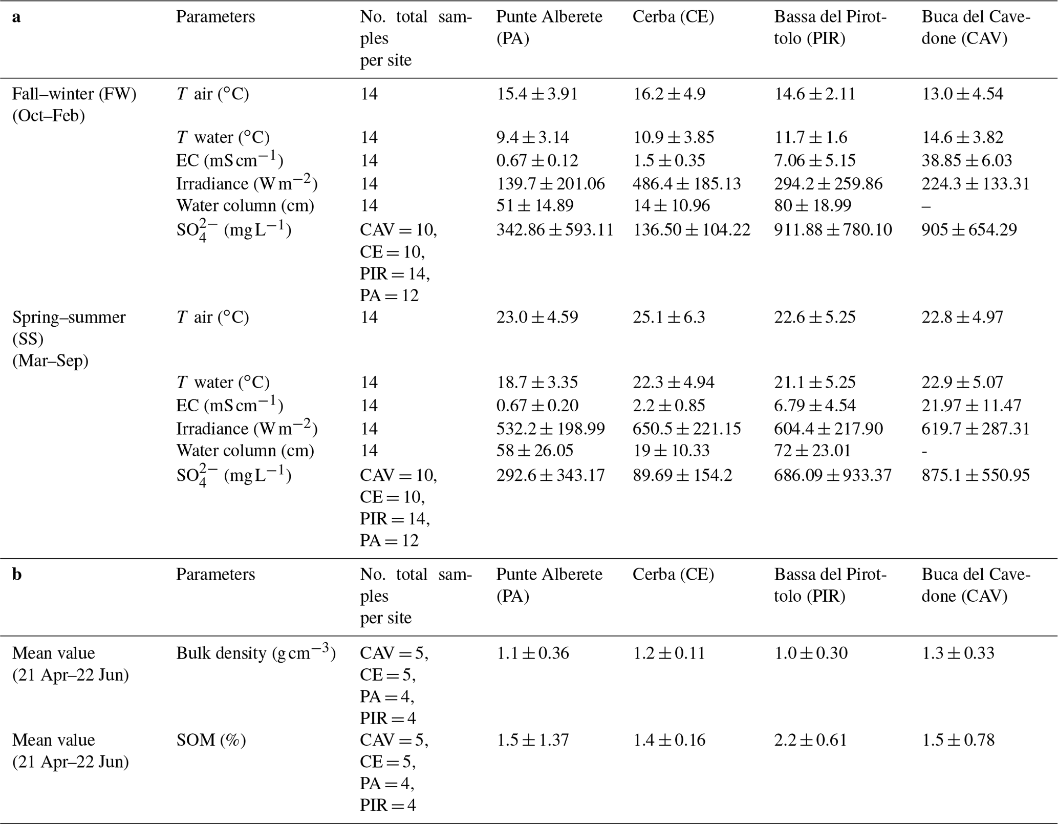
Table 1 a Mean seasonal values ± standard deviation for recorded environmental parameters. No values for the water column in CAV were collected. b Mean values of bulk density and organic matter content were measured on soil cores.

3 Results

3.1 GHG fluxes and environmental variables

3.1.1 Environmental variables

For a general overview, data are divided into two groups, i.e., those collected in the fall–winter (FW) period and those collected in the summer–spring (SS) period (Table 1).

PA is always the site with the coldest water temperature (9.4 ^∘C in FW and 18.7 in SS), and the lowest water EC value (0.67 mS cm⁻¹ in both FW and SS) of the whole study area for both seasons. This site also always has the second-highest water column levels (51 cm in FW and 58 cm for SS) of the overall study area and the lowest irradiance values (139.7 W m⁻² in FW and 532.2 W m⁻² in SS).

CE, while still being a freshwater site, has a higher salinity than PA during both seasons (1.49 mS cm⁻¹ in FW and 2.24 mS cm⁻¹ in SS) and records the highest mean water temperature in SS (22.3 ^∘C). In the same period, also air temperature had one of the highest values recorded during the field campaign (25.1 ^∘C). CE is also the site where the mean water column is the lowest (14 cm in FW and 19 cm in SS), and the mean irradiance is the highest (486.4 W m⁻² in FW and 650.5 W m⁻² in SS) during both SS and FW. CE has the lowest mean soil content of organic matter (1.4 %) of the four sites.

PIR has the second-highest value of EC (7.06 mS cm⁻¹ in FW and 6.79 mS cm⁻¹ in SS) of all four sites during both seasons, and it has the second-highest concentration of ${\mathrm{SO}}_{\mathrm{4}}^{\mathrm{2}-}$ during SS (640.8 mg L⁻¹). PIR is also the site with the highest water column level during both seasons (80 cm in FW and 72 cm in SS) and the highest mean content of organic matter in the sediments (2.2 %) but the lowest bulk density (1 g cm⁻³).

CAV is the site with the highest EC of all studied areas during both seasons (38.85 mS cm⁻¹ in FW and 21.97 mS cm⁻¹ in SS) and the highest concentration of ${\mathrm{SO}}_{\mathrm{4}}^{\mathrm{2}-}$ during SS (875.1 mg L⁻¹). Here, the mean air temperature is the lowest of all sites during FW (13 ^∘C). For this site, no record of the water column level is collected, due to fluxes being always under the detection limit of the instrument.

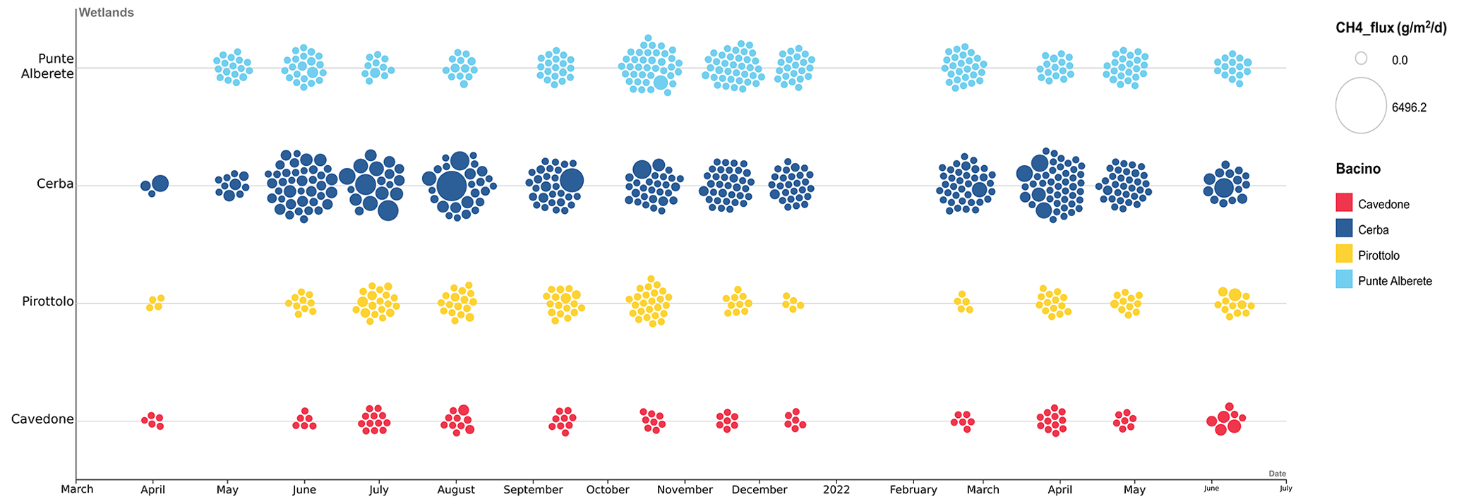
Figure 2 Bubble graph representing CH₄ fluxes from June 2021 to July 2022 in the four studied wetlands. During January 2022 it was not possible to perform measurements due to frosting.

3.1.2 GHG fluxes

Figure 2 shows the seasonal pattern in the CH₄ emissions recorded through the sampling campaign. Higher fluxes are recorded throughout the spring and summer months, declining in winter and fall. Also, fluxes in freshwater environments (PA and CE) are often higher than those recorded in brackish environments (PIR and CAV).

Table 2 Seasonal values for CO₂ and CH₄ fluxes. SD: standard deviation; CV(%): coefficient of variation.

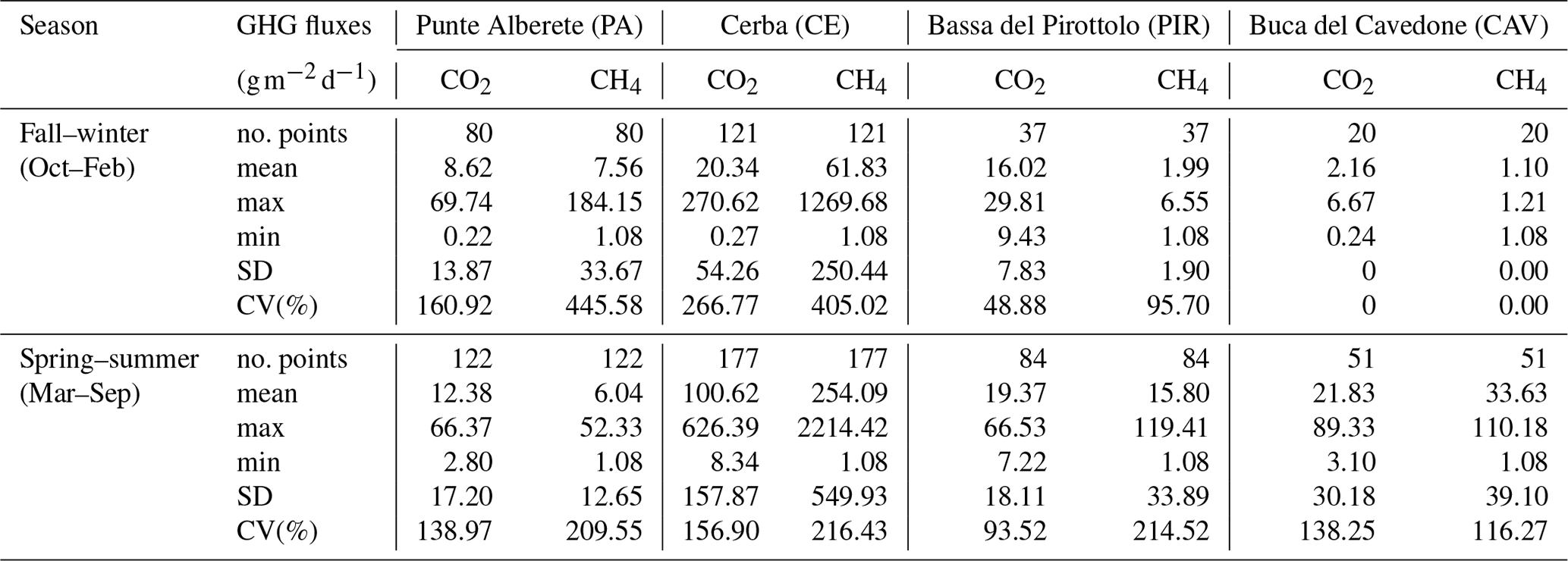
CH₄ and CO₂ fluxes in PA are always lower than those recorded in CE, while both sites are characterized by the presence of freshwater. During SS in particular, PA has the lowest mean flux of CH₄ of the whole study area (6.04 $\mathrm{g}{\mathrm{m}}^{-\mathrm{2}}{\mathrm{d}}^{-\mathrm{1}}$), while CE is the highest (254.09 $\mathrm{g}{\mathrm{m}}^{-\mathrm{2}}{\mathrm{d}}^{-\mathrm{1}}$) (Table 2).

The highest mean values of CH₄ and CO₂ for both seasons are recorded in CE (Table 2). Mean CH₄ fluxes account for 61.83 $\mathrm{g}{\mathrm{m}}^{-\mathrm{2}}{\mathrm{d}}^{-\mathrm{1}}$ during the FW and 254.09 $\mathrm{g}{\mathrm{m}}^{-\mathrm{2}}{\mathrm{d}}^{-\mathrm{1}}$ during the SS, CO₂ fluxes accounted for 20.34 $\mathrm{g}{\mathrm{m}}^{-\mathrm{2}}{\mathrm{d}}^{-\mathrm{1}}$ during the FW, and 100.62 $\mathrm{g}{\mathrm{m}}^{-\mathrm{2}}{\mathrm{d}}^{-\mathrm{1}}$ during the SS (Table 2).

In PIR, CH₄ fluxes are 1.99 $\mathrm{g}{\mathrm{m}}^{-\mathrm{2}}{\mathrm{d}}^{-\mathrm{1}}$ in FW and 15.80 $\mathrm{g}{\mathrm{m}}^{-\mathrm{2}}{\mathrm{d}}^{-\mathrm{1}}$ in SS, among the lowest during SS, except for PA. CO₂ fluxes are 16.02 $\mathrm{g}{\mathrm{m}}^{-\mathrm{2}}{\mathrm{d}}^{-\mathrm{1}}$ in FW, the lowest record for the season, and 19.37 $\mathrm{g}{\mathrm{m}}^{-\mathrm{2}}{\mathrm{d}}^{-\mathrm{1}}$ in SS (Table 2).

CAV is the site with both the highest salinity and the lowest emissions. CH₄ and CO₂ fluxes are the lowest during the FW with a recorded mean value of 1.10 $\mathrm{g}{\mathrm{m}}^{-\mathrm{2}}{\mathrm{d}}^{-\mathrm{1}}$ and 2.16 $\mathrm{g}{\mathrm{m}}^{-\mathrm{2}}{\mathrm{d}}^{-\mathrm{1}}$, respectively.

3.2 Principal component analysis

3.2.1 PCA results

PCA is performed considering separately CO₂ and CH₄ fluxes to better investigate their correlation with the environmental variables and the two principal components that better explain the most variance percentages.

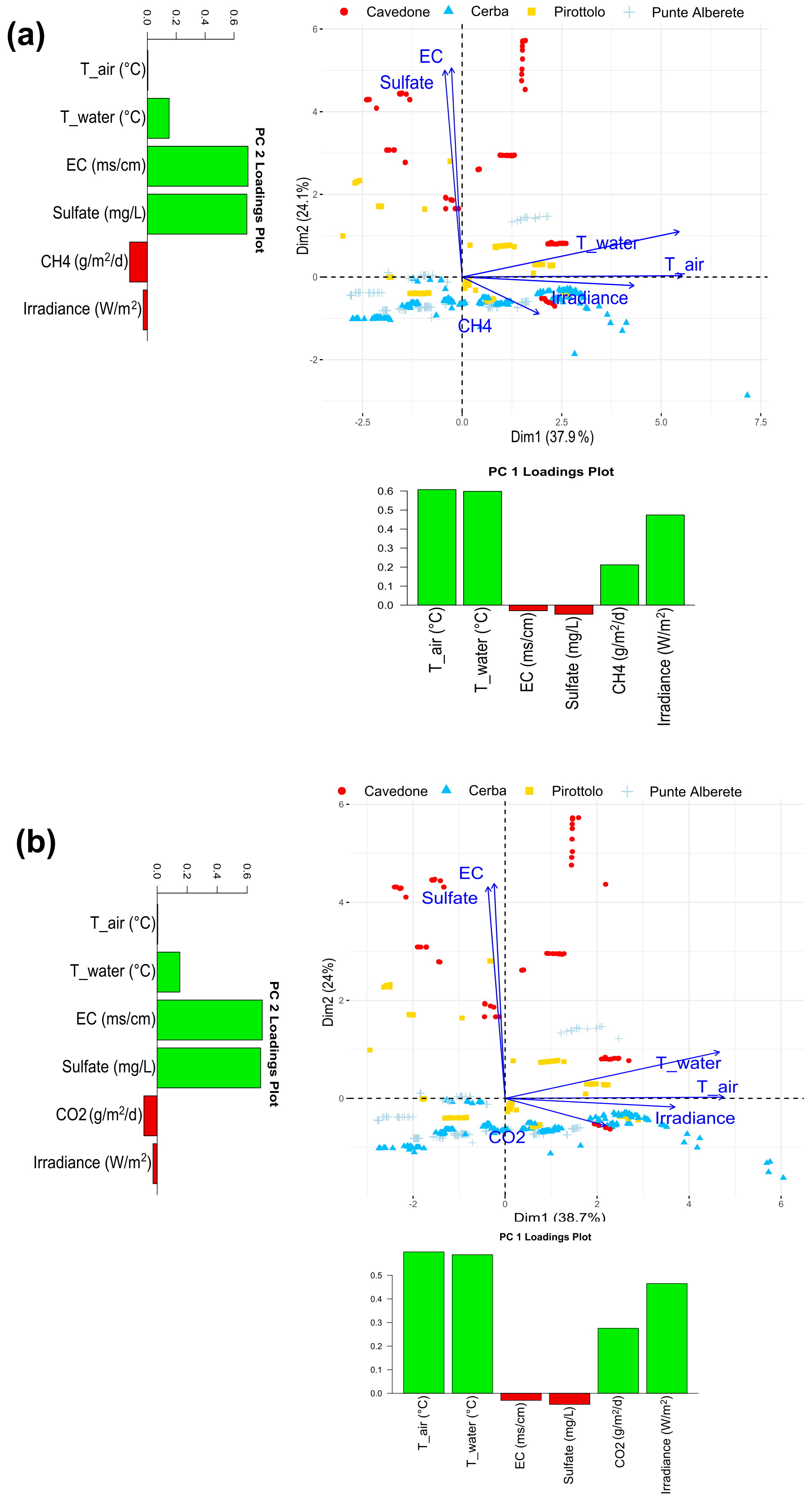
Figure 3 Biplot representing PC1 and PC2 for (a) CH₄ fluxes and the observed environmental variables and (b) CO₂ fluxes and the observed environmental variables. Along the axis of the biplot, the histograms report the loadings values for the respective component.

Table 3 Values for CO₂ and CH₄ fluxes measured from standing waters. SD: standard deviation; CV (%): coefficient of variation; no. points: points fluxes measured.

In this section, PCA on fluxes from soils and water is presented jointly. Figure 3 shows the plots of PC1 and PC2 for CH₄ (Fig. 3a) and CO₂ (Fig. 3b) and all measured environmental variables. For CH₄ in particular the two components explain 63.9 % of the total variance, and specifically PC1 explains 38.5 % and PC2 25.4 % of variance (Fig. S3 in the Supplement). Water temperature, air temperature, and irradiance are clustered in one group to the right, indicating close relation among each other. They all increase as the PC1 increases, while they are barely affected by PC2. CH₄ emissions also increase as the PC1 increases, but they increase as PC2 decreases. On the contrary, both salinity and ${\mathrm{SO}}_{\mathrm{4}}^{\mathrm{2}-}$ increase as PC2 increases, showing a limited contribution of PC1 (Fig. 3a). This result shows a positive correlation between CH₄ production, water and air temperature, and irradiance, whereas CH₄ production is negatively correlated to salinity (Fig. S7 in the Supplement).

Points in the biplot represent the field measurements. Plotted in Fig. 2a, points in red represent data collected at CAV and have in general higher PC2 values than those collected in the other three study sites. Their distribution goes accordingly with the strong positive correlation between PC2 and salinity and CAV presenting higher salinity values than the other sites. Similarly, CAV appears to be the site with the lowest CH₄ emissions in the FW period (Table 2), given that CH₄ emissions increase as salinity decreases. We conclude that measurements performed in brackish environments such as CAV are characterized by generally lower emissions if we compare them to those measured in freshwater sites.

When the PCA is performed on CO₂ and the observed environmental variables, PC1 explains 38.6 % and PC2 24 % of the total variance, accounting together for 62.6 % of the total variance (Fig. S4 in the Supplement). The results are shown in Fig. 2b. Similarly to the results obtained for CH₄, water and air temperature and irradiance cluster together, contributing highly to PC1. These variables also show a positive correlation with CO₂ production and are highly correlated within themselves (Fig. S8 in the Supplement). On the contrary, salinity is displayed along PC2 and shows a negative correlation with CO₂ emissions.

3.3 GHG fluxes from flooded areas

Considering exclusively fluxes measured on flooded areas, i.e., areas permanently or seasonally characterized by the presence of water, Table 3 summarizes the results.

In PA, CH₄ fluxes are relatively low (5.04 $\mathrm{g}{\mathrm{m}}^{-\mathrm{2}}{\mathrm{d}}^{-\mathrm{1}}$) with moderate variability, as indicated by the coefficient of variation (CV) of 422.23 %. The maximum CH₄ flux (228.49 $\mathrm{g}{\mathrm{m}}^{-\mathrm{2}}{\mathrm{d}}^{-\mathrm{1}}$) measured at this location suggests occasional spikes in emissions. CE exhibits high mean CH₄ flux (196.98 $\mathrm{g}{\mathrm{m}}^{-\mathrm{2}}{\mathrm{d}}^{-\mathrm{1}}$) along with a CV of 341.95 %. PIR shows a mean CH₄ flux of 12.27 $\mathrm{g}{\mathrm{m}}^{-\mathrm{2}}{\mathrm{d}}^{-\mathrm{1}}$, which is comparable to PA and lower than CE. Table 3 includes the values recorded at CAV even though their number is smaller than the ones obtained at other sites and most values are very low, often close to the limits of the instrument detection, therefore influencing the statistical significance of the dataset. Therefore, we excluded this dataset from the analyses described in the next chapters.

The CH₄ flux dynamics underscore the significant variations in methane emissions across the different wetland locations. CE stands out with the highest mean and maximum values of CH₄ fluxes and presenting high variability. PA and PIR also exhibit variability in CH₄ emissions but with lower mean and maximum values.

In PA, the mean CO₂ flux is relatively low (5.67 $\mathrm{g}{\mathrm{m}}^{-\mathrm{2}}{\mathrm{d}}^{-\mathrm{1}}$), and the CV is 86.25 %, indicating moderate variability. The maximum CO₂ flux recorded at PA is 47.39 $\mathrm{g}{\mathrm{m}}^{-\mathrm{2}}{\mathrm{d}}^{-\mathrm{1}}$, suggesting occasional picks. CE exhibits a much higher mean CO₂ flux, equal to 71.42 $\mathrm{g}{\mathrm{m}}^{-\mathrm{2}}{\mathrm{d}}^{-\mathrm{1}}$. The maximum CO₂ flux recorded in CE is exceptionally high at 1355.04 $\mathrm{g}{\mathrm{m}}^{-\mathrm{2}}{\mathrm{d}}^{-\mathrm{1}}$, indicating the presence of significant emission spikes. PIR has a mean CO₂ flux of 15.47 $\mathrm{g}{\mathrm{m}}^{-\mathrm{2}}{\mathrm{d}}^{-\mathrm{1}}$. The maximum CO₂ flux recorded is 142.62 $\mathrm{g}{\mathrm{m}}^{-\mathrm{2}}{\mathrm{d}}^{-\mathrm{1}}$, indicating intermittent peaks in CO₂ emissions.

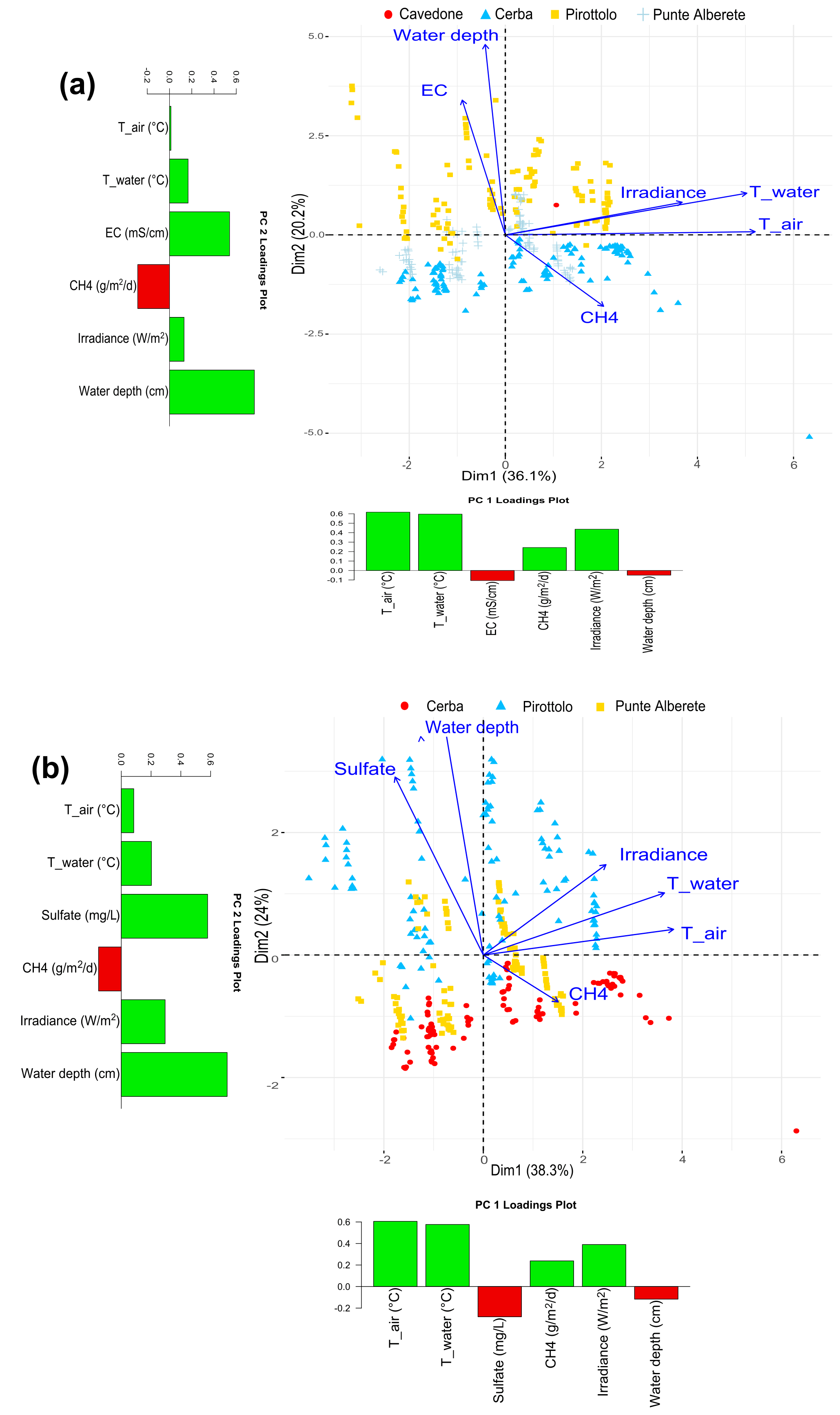
Figure 4 Biplot representing PC1 and PC2 exclusively for flooded areas for (a) CH₄ fluxes and the observed environmental variables including salinity and excluding sulfate, and (b) CH₄ fluxes and the observed environmental variables including sulfate and excluding salinity. Along the axis of the biplot, the histograms report the loadings values for the respective component.

3.3.1 PCA results

For the dataset presented in Table 3, PCA is performed considering CH₄ fluxes and all environmental variables, alternately excluding sulfate and EC (Fig. 4). The analyses are repeated for CO₂ fluxes.

PCA performed on CH₄ fluxes is influenced by water column height and ${\mathrm{SO}}_{\mathrm{4}}^{\mathrm{2}-}$ concentrations: PC1 and PC2 explain 38.3 % and 24 % of the variance, respectively, for a total of 62.3 % of the total variance (Fig. S11 in the Supplement). Similarly, considering EC and water column height in performing the PCA, it is found that PC1 accounts for 36.1 % of the variance and PC2 for 20.1 %, for a total of 56.2 % of cumulative variance.

Figure 4a and b show that air, water temperature, and irradiance vectors cluster together on the right of the graph, suggesting a strong correlation among them. On the opposite side, along PC2, salinity, sulfate, and water column increase as PC2 increases, while they are negatively correlated to PC1. CH₄ emissions increase as PC1 increases while decreasing as PC2 increases, therefore showing a negative correlation with both EC and water depth. Looking at the distribution of the scores, representing field observations, their variability is controlled by EC and ${\mathrm{SO}}_{\mathrm{4}}^{\mathrm{2}-}$ concentrations, water column height, and CH₄ emissions. All measurements collected in PIR (characterized by brackish waters) fall into the higher part of the graph, where PC2 values are positive, whereas those collected in CE (shallow and slightly fresh waters) cluster in the lower section of the graph, and finally observations collected in PA (deep and fresh waters) are in the midsection of the graph.

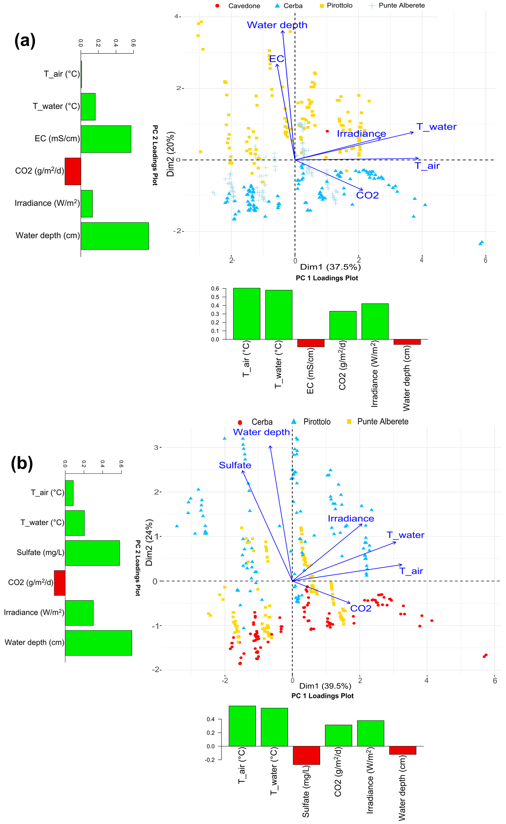
Figure 5 Biplot representing PC1 and PC2 exclusively for flooded areas for (a) CO₂ fluxes and the observed environmental variables including salinity and excluding sulfate, and (b) CO₂ fluxes and the observed environmental variables including sulfate and excluding salinity. Along the axis of the biplot, the histograms report the loadings values for the respective component.

When CO₂ fluxes are considered together with sulfate and water column height (Fig. 5a and b), PC1 and PC2 explain, respectively, 39.5 % and 24 % of dataset variance, for a total of 63.5 % of the cumulative variance (Fig. 5b). When performing the same analysis on the dataset considering EC and water depth, the first two components explain a total of 57.5 % of the variance. PC1 accounts for 37.5 % of the variance and PC2 for 20 % (Fig. S12 in the Supplement). In both analyses on CH₄ and CO₂ fluxes, the presence of sulfate can better describe the dataset. The results from the biplot (Fig. 5a and b) are similar to those obtained for CH₄ (Fig. 4a and b). The vectors of air, water temperature, and irradiance are correlated positively with CO₂ production and distributed along PC1 (Fig. 5b). EC, sulfate, and water depth column follow the PC2 axis and have a negative correlation with CO₂ emissions.

3.3.2 Water column effect

The effect of water temperature and water column height on CH₄ and CO₂ flux distribution is examined and shown in Fig. 6a–b and 6c–d, respectively. High fluxes occur when the water height is lower than 50 cm, tendentially with high temperatures. For larger water heights, the emissions are small despite the presence of high temperatures.

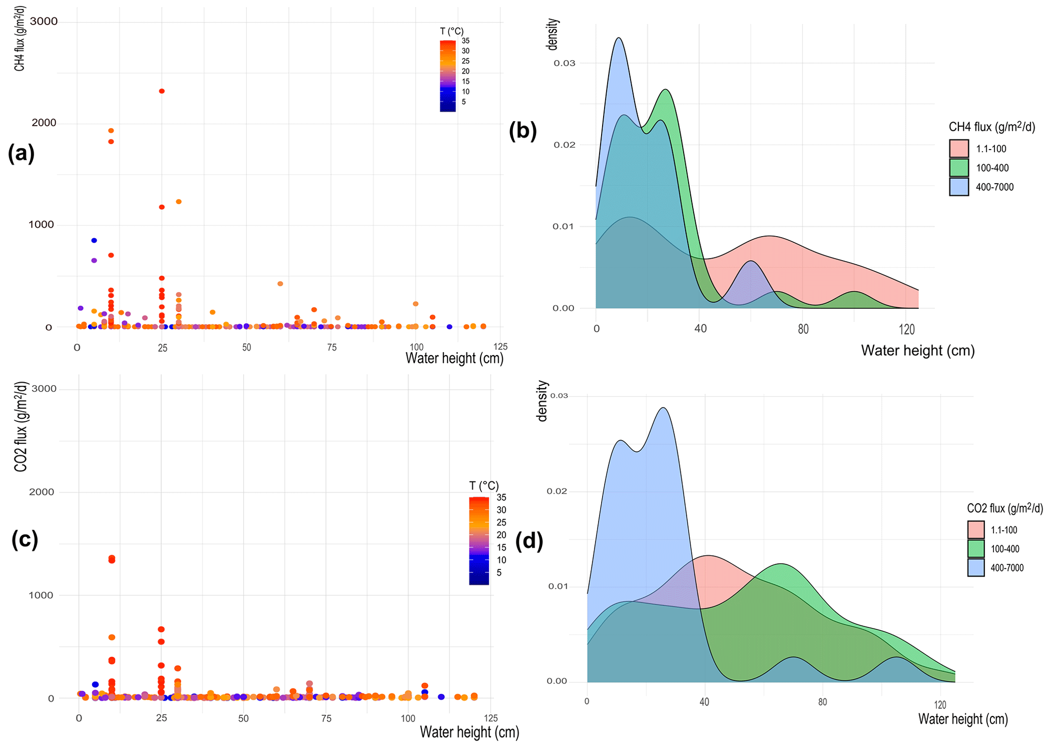
Figure 6 (a, c) Heat maps showing flux distribution depending on water column height; the colors indicate the water temperature; (b) and d) represent the probability density function (PDF) showing at which water columns height is more probable to observe high (blue), medium (green), and low (pink) fluxes. The top panels are for CH₄ fluxes, while the bottom panels are for CO₂ fluxes.

The probability density function (PDF) in Fig. 6b shows the probability of observing certain ranges of CH₄ fluxes for different water column heights. Results show that low fluxes of CH₄ (i.e., 1–100 $\mathrm{g}{\mathrm{m}}^{-\mathrm{2}}{\mathrm{d}}^{-\mathrm{1}}$) are observed in both shallow and deep waters, but medium and high fluxes (i.e., 100–7000 $\mathrm{g}{\mathrm{m}}^{-\mathrm{2}}{\mathrm{d}}^{-\mathrm{1}}$) are observed only when the water column height is less than 50 cm deep. To further confirm these results, data are grouped into two classes: deep (> 50 cm) and shallow (< 50 cm) waters. A Mann–Whitney test is run on the two data classes, returning a p value of $\mathrm{4.66}\times {\mathrm{10}}^{-\mathrm{6}}$ for CH₄ (Fig. S15 in the Supplement), confirming that the two classes are statistically different and that there is a threshold depth below which the wetland becomes an important source of CH₄.

The same analysis is applied to CO₂ fluxes (Fig. 6c). The heat map shows a behavior similar to CH₄, with higher fluxes recorded only for low waters (Fig. 6c), independently of the water temperature. The PDF in Fig. 6d confirms that low fluxes of CO₂ (i.e., 1–100 $\mathrm{g}{\mathrm{m}}^{-\mathrm{2}}{\mathrm{d}}^{-\mathrm{1}}$) are observed in both shallow and deep waters, while higher fluxes (i.e., 100–1300 $\mathrm{g}{\mathrm{m}}^{-\mathrm{2}}{\mathrm{d}}^{-\mathrm{1}}$) are observed only when the water column height is less than 50 cm deep. However, differently from the analysis performed on CH₄ measurements, the Mann–Whitney test shows a non-significant difference for the two water height classes > 50 cm and < 50 cm of water depth for CO₂ emissions (p = 0.82 for CO₂) (Fig. S16 in the Supplement).

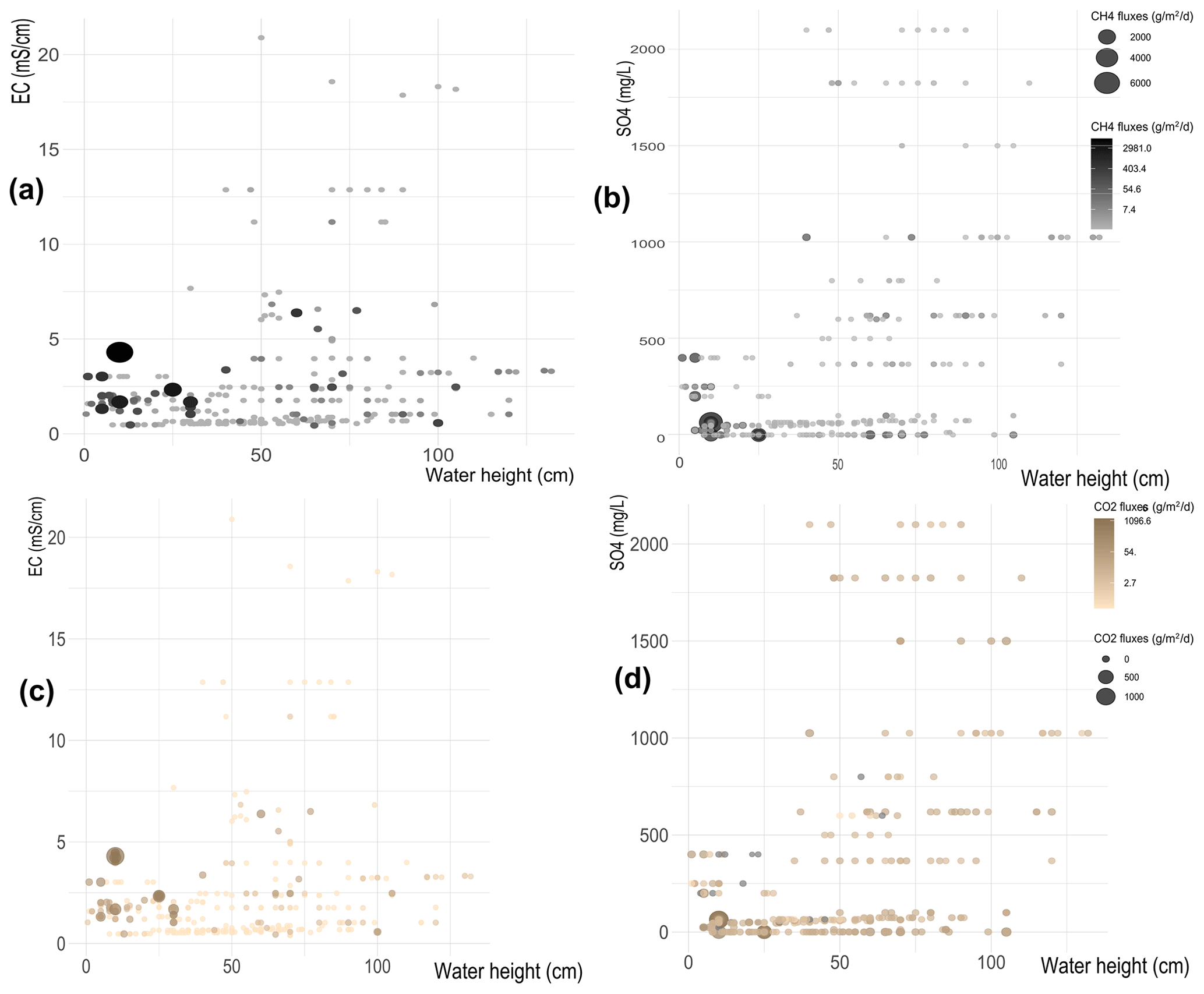
Figure 7 Heat maps comparing the CH₄ flux distribution depending on water column height and EC values (a) and ${\mathrm{SO}}_{\mathrm{4}}^{\mathrm{2}-}$ concentrations (b). Heat maps comparing the CO₂ flux distribution depending on water column height and EC values (c) and ${\mathrm{SO}}_{\mathrm{4}}^{\mathrm{2}-}$ concentrations (d).

When the influence of salinity and sulfates is considered, both heat maps in Fig. 7a and b show that higher CH₄ emissions are concentrated in the low-left portion of the graphs, i.e., at water heights smaller than 50 cm and low EC and sulfate concentrations, and this happens for both EC and sulfates even though it is more pronounced for sulfate than for EC. When the water level is higher than 50 cm, CH₄ emissions are small, whatever EC and ${\mathrm{SO}}_{\mathrm{4}}^{\mathrm{2}-}$ concentrations were measured. We notice that there are no data available for the case of low water-high EC or for low water-high sulfates; we speculate because our study sites do not include shallow salted wetlands.

If we compare Figs. 6a, b, and 7b, we notice that independently of T, EC and ${\mathrm{SO}}_{\mathrm{4}}^{\mathrm{2}-}$, emissions of CH₄ are low for water heights larger than 50 cm.

Similar results are obtained for CO₂ fluxes. Figure 7c and d show that high CO₂ emissions are only recorded when the water height is lower than 50 cm, while in deeper waters the CO₂ emissions are always small, independently of EC and sulfate concentrations. In line with the results shown for CH₄ fluxes, also in the case of CO₂, we confirm that high values of T, EC, and ${\mathrm{SO}}_{\mathrm{4}}^{\mathrm{2}-}$ do not influence CO₂ emissions (Fig. 6c, d and 7c, d), which remain small when the water height exceeds 50 cm. As already stated, no data were available for low-salt waters.

4 Discussion

This study explores how the spatial and temporal variability of environmental drivers such as water and air T, salinity, irradiance, and inundation levels influence CH₄ and CO₂ emissions in four adjacent coastal wetlands.

In general, when all data collected on flooded areas as well as on wet soils were considered, lower fluxes of CH₄ were observed in meso-/polyhaline environments (PIR and CAV), compared to what was observed in freshwater sites (PA and CE) (Table 1). PIR and CAV are the richest in ${\mathrm{SO}}_{\mathrm{4}}^{\mathrm{2}-}$ (Fig. 1), an ion that can be used by sulfate-reducing bacteria as a terminal electron acceptor during anaerobic decomposition (Hackney and Avery, 2015; Zhou et al., 2022). In contrast to methanogenesis, the sulfate reduction process is naturally favored since sulfate-reducing bacteria compete more efficiently for available substrates, like acetate and hydrogen, than methanogenic bacteria (Lovley and Klug, 1986).

Our results confirm the strong inhibiting function of EC and sulfates. CH₄ emissions are found to be negatively correlated to EC and ${\mathrm{SO}}_{\mathrm{4}}^{\mathrm{2}-}$ (Fig. S7), which is consistent with the existing literature on coastal wetlands (Hines, 1996; Poffenbarger et al., 2011; Chen et al., 2018).

On average from PCA results, it is possible to observe two groups of environmental controls: (i) one aggregated component related to seasonality, grouping air and water T and irradiance, with a strong positive control on GHG emissions, and (ii) one related to the hydrological aspect of the wetlands represented by EC, ${\mathrm{SO}}_{\mathrm{4}}^{\mathrm{2}-}$, and water column height with a significative negative impact on GHG production.

CH₄ emissions show a seasonal pattern and generally are higher in the warmer season (Emery and Fulweiler, 2014; Al-Haj and Fulweiler, 2020), as shown in Fig. 2 with the highest values recorded in summer (Table 2). In general, CH₄ and CO₂ emissions are positively correlated with air and water temperature and irradiance. Temperature directly affects CH₄ production stimulating methanogenic kinetics (Zinder and Koch, 1984) (Fig. 3a). In fact, methanogen bacteria are reported to be generally mesophilic, with a growth temperature between 30 and 40 ^∘C (Zinder, 1993).

CO₂ fluxes are also correlated to temperature and irradiance (Fig. S8), highlighting a seasonal pattern with higher fluxes in the spring–summer season. It is known that CO₂ fluxes mainly come from soil respiration, including roots and microbial activity (Rustad et al., 2000). Additionally, methanotrophs in the soil surface layer may be able to oxidize part of the CH₄, and aerobic microbes can use more O₂ to oxidize organic matter. This condition is observed in CE (Table 2), which accounts for the overall highest mean fluxes of CO₂ during spring and summer.

CO₂ and CH₄ emissions are also linked to vegetation composition and organic matter presence. In our case, the second highest mean fluxes of CO₂ are measured at PIR (Table 2). This can be mainly related to the high presence in this area of Phragmites australis,which is reported to be particularly effective in transporting gas through its structures, from the submerged soil to the atmosphere (Martin and Moseman-Valtierra, 2015). Moreover, the high presence of Phragmites has the potential of increasing C turnover rates, providing higher rates of primary production that may be offset by enhanced rates of plant litter decomposition (Duke et al., 2015). Anyway, this could also explain the high percentage of soil organic matter (SOM) measured at the PIR site (Table 1).

When we concentrate on flooded areas examining only fluxes collected over standing waters, we observe some important differences. Even though the principal components are pretty much in line with those determined for the entire dataset (Figs. 4 and 5), we find a strong influence of water depth on CH₄ and CO₂ emissions. Figures 6 and 7 show that there is a water column height threshold that separates low from high emissions. It is known that CH₄ emission from wetlands depends, in part, on the balance between methanogenesis and CH₄ oxidation. Methanogenesis occurs in the submerged, anoxic soil layers, and so it depends on the vertical extension of the saturated zone determined by the water table level. When the level of the water table increases reaching the soil surface, it creates anaerobic conditions favoring methanogenesis, which is a strictly anaerobic process (Mander et al., 2011; Calabrese et al., 2021). After being produced, CH₄ can be transported vertically or horizontally. The nature of the transport pathway (length, direction, presence of methanotrophs) determines the potential for CH₄ to be oxidized or, on the contrary, released as it is in the atmosphere (Dean et al., 2018). The constant presence of a deep water column on top of sediments creates the temporal and spatial condition for methanotroph bacteria to consume CH₄ in the water column (Henneberger et al., 2015; Sawakuchi et al., 2016), resulting in decreasing rate of CH₄ fluxes, as shown in Fig. 6. This agrees with the case of PA (Table 2) where the lower CH₄ fluxes compared to those in CE could be linked to a deep and permanent water column that may act as a physical barrier to CH₄ diffusion (Cheng et al., 2007). The ensemble of these processes creates a critical zone where the availability of methanogenic substrates, anoxic portions of soil, and gas transport compete in creating either a favorable or unfavorable environment for CH₄ emissions (Calabrese et al., 2021). A further increase in the water column level, however, is more likely to decrease CH₄ production limiting plant growth and available substrate for decomposition (Calabrese et al., 2021)

Even though these processes are well known, in the literature it is not clear whether the CH₄ emissions steadily increase with decreasing the water depth or whether, on the contrary, there is a threshold in water column height that separates emitting condition from no-emission condition. For the first time regarding temperate coastal wetlands, our results suggest that there is a critical threshold of water height, which, in our case, corresponds to about 50 cm below which wetlands release large quantities of CH₄ to the atmosphere. Figure 6a and b shows that high CH₄ emissions are recorded only where the water height is lower than this threshold as further confirmed by the Mann–Whitney test performed on shallow and deep waters (Fig. S15). This process explains, for instance, the differences in observed emissions between CA and PA where in CA, CH₄ emissions are 8 times higher than those measured in PA (Table 2). These two sites have comparable salinity and temperature but differ greatly in their inundation levels (54 cm in PA and 18 cm in CE).

As for the case of CO₂ emissions, the behavior is similar for CH₄; however, the Mann–Whitney test suggests that there is no significant difference between CO₂ emissions coming from waters higher and lower than 50 cm (Fig. S16). Bacteria responsible for CH₄ oxidation are less limited by exposure to anoxic conditions than methanogenic bacteria to oxic (Roslev and King, 1996), so CO₂ fluxes can be expected at low as well as at high water levels. Moreover, CO₂ emissions in seawater are higher than in freshwater because of the increased availability of ${\mathrm{SO}}_{\mathrm{4}}^{\mathrm{2}-}$ to serve as a terminal electron acceptor in anaerobic microbial respiration (Zhao et al., 2020). Finally, there is a relation between oxidation mechanisms and CH₄ fluxes depending on the efficiency of the gas transport within the ecosystem (Torres-Alvarado et al., 2005). In shallow waters, CH₄ diffusion is favored by low pressure and oxidation performed by oxidizing bacteria is limited (Weber et al., 2019). On the contrary, CH₄ oxidation is favored in deeper water, which slows down the diffusion of CH₄ and allows it to accumulate, providing more substrate for CH₄-oxidizing bacteria to grow and consume CH₄ (Weber et al., 2019). The combination of these processes may explain why no significant differences of CO₂ emissions were observed in waters deeper or shallower than 50 cm, while significant differences are observed for CH₄ emissions.

Concluding, our results suggest that, above a certain threshold, the water depth is the main limiting factor of GHG emissions and at our study sites such a threshold is 50 cm. When water is deeper than the threshold, the emission of CH₄ and CO₂ is very limited, regardless of the temperature being high or low (Fig. 5), but also independently of EC and sulfate concentrations (Fig. 7). High CH₄ emissions are observed only in shallow waters with small EC and sulfate concentrations (Fig. 7).

The results presented in this study are of relevance for the water management of this and other wetland areas that are controlled and managed by authorities. Knowing that the water depth should never be lower than 50 cm to minimize GHG emissions is crucial information for proper management of the area.

Methanogenesis is a complex interplay of environmental factors and site-specific conditions (Kotsyurbenko et al., 2019), and the inclusion of more variables in the analyses may improve the results allowing a more comprehensive understanding of the processes investigated in this research. In particular, vegetation, primary productivity, and chlorophyll α can influence the organic matter supplied to sediments, influencing methanogenesis rates in wetland sediments both in freshwater and saltwater ecosystems (Grasset et al., 2018; Huertas et al., 2019). Another aspect that should be further considered is that the methanogenesis process depends on soil characteristics found in wetlands. There is a strong association between the quantity of methanogenic archaea and the concentration of organic C in wetland soils, and the amount of it influences the population of methanogens in wetland ecosystems (Liu et al., 2019). Because it has an impact on the soil capacity to oxidize CH₄, bulk density is a crucial variable in the management of GHG emissions in wetlands. The capacity of aerobic soil to oxidize CH₄ is reduced when the soil is submerged, leading to high CH₄ concentrations in these wetlands (Zhao et al., 2020).

Research that focuses on microbial community structure, the interaction between microbial communities and carbon-functional composition, and the ecological factors influencing both microbial communities and carbon-functional composition is essential to better understand the complex methanogenesis process in coastal environments.

Future research will be conducted to accomplish these goals, primarily concentrating on biogeochemistry and the organization of microbial communities, and promoting a comprehensive knowledge of the complex processes that underlie methanogenesis in coastal environments.

5 Conclusions

This study aims to identify the driving and limiting environmental factors for CH₄ and CO₂ production in temperate coastal wetlands with varying water salinity. It shows, for the first time, that CH₄ and CO₂ emissions in the Po River Delta Natural Park exhibit strong variations within a few kilometers and during different periods of the year, indicating a strong dependence on seasonality. Temperature and irradiance strongly influence CH₄ emissions from water and soil, resulting in higher rates during summer and spring.

We observe a significant decrease in CH₄ emissions when the water depth exceeds the critical threshold of 50 cm. Regardless of the water salinity, the average CH₄ flux is 5.04 $\mathrm{g}{\mathrm{m}}^{-\mathrm{2}}{\mathrm{d}}^{-\mathrm{1}}$ in freshwater environments and 12.27 $\mathrm{g}{\mathrm{m}}^{-\mathrm{2}}{\mathrm{d}}^{-\mathrm{1}}$ in brackish settings. In contrast, when the water depth is less than 50 cm, CH₄ emissions strongly increase to an average value of 196.98 $\mathrm{g}{\mathrm{m}}^{-\mathrm{2}}{\mathrm{d}}^{-\mathrm{1}}$ in freshwater areas. Same behaviors are observed for CO₂ fluxes, although they are statistically non-significant. Additionally, temperature and irradiance exert a strong influence on CH₄ emissions from both water and soil, resulting in higher emissions in summer and spring seasons than in the cold season.

Our results suggest that CH₄ oxidation by oxidizing bacteria is limited in shallow waters due to enhanced CH₄ diffusion, while CH₄ oxidation is more pronounced in deep waters, resulting in larger CO₂ emissions. The combination of these processes may explain why water depth is a key limiting factor of CH₄ emissions, while CO₂ emissions remain constant regardless of the water depth.

For water column depths less than 50 cm, we identify additional constraining factors, particularly the inhibitory roles of salinity and sulfate concentrations on CH₄ emissions, although specific threshold values for these variables could not be established, highlighting the complexity of the processes at play.

Considering the impacts of climate change, carefully studying temperate coastal wetlands and understanding the dynamics of CH₄ and CO₂ production are critically important to develop targeted management measures to reduce emissions from wetlands. These strategies are essential in the collective effort to meet climate targets, such as the 2030 Agenda for Sustainable Development and the objectives of the Paris Agreement on Climate Change (European Commission, 2020).