Lawns and meadows in urban green space – a comparison from perspectives of greenhouse gases, drought resilience and plant functional types

Today, city planners design urban futures by considering environmental degradation and climate mitigation. Here, we studied the greenhouse gas fluxes of urban lawns and meadows and linked the observations with plant functional types and soil properties. In eight lawns and eight meadows in the Helsinki metropolitan area, Finland, carbon dioxide (CO₂), methane (CH₄) and nitrous oxide (N₂O) fluxes were measured using manual chambers, and plant functional types were recorded. Four of these sites, i.e. an irrigated lawn, an old mesic meadow, a non-irrigated lawn and a young dry meadow, were more intensively studied in 2021–2022. The process-based ecosystem model JSBACH was utilized together with the momentary observations collected approximately every second week on CO₂ exchange to quantify the annual carbon (C) balance of these sites. On the remaining sites, we studied the initial dynamics of conversion from lawns to meadows by transforming parts of lawns to meadows in late 2020 and conducting measurements from 2020 to 2022. The mean photosynthetic production (GPP) of the irrigated lawn and mesic meadow was the highest in this study, whereas the dry meadow had the lowest GPP. The studied lawns were stronger C sinks compared to the meadows. However, the net exchange values were uncertain as the soils were not in equilibrium with the vegetation at all sites, which is common for urban habitats, and modelling the heterotrophic emissions was therefore challenging. The conversion from a lawn to a meadow did not affect the fluxes of CH₄ and N₂O. Moreover, the mesic meadow was more resistant to drought events than the non-irrigated lawn. Lastly, the proportion of herbaceous flowering plants other than grasses was higher in meadows than in lawns. Even though social and economic aspects also steer urban development, these results can guide planning when considering environmentally friendlier green spaces and carbon smartness.

1 Introduction

The impacts of climate change and environmental degradation are increasingly evident. These crises are interlinked with each other by feedbacks, and as climate change threatens species and ecosystems, the loss of biodiversity and degradation of ecosystems also affect the climate system. Therefore, understanding the role of various ecosystems in regulating climate and supporting biodiversity within the land-use sector is crucial. It is also important to identify land management practices that can effectively mitigate climate and other environmental crises simultaneously. Well-known management practices for the land-use sector include, for example, conservation and restoration and integrated land-use planning, taking into account the relationships between different land uses (Niemelä et al., 2010; Pörtner et al., 2021).

In the urban context, green spaces not only sequester atmospheric carbon (C) but also provide vital ecosystem services, such as cooling, recreational values, purification of air and water, and reducing the risk of flooding (Niemelä et al., 2010; Belmeziti et al., 2018; Lampinen et al., 2021; Shen et al., 2023). Cities actively seek optimal green space planning and management practices to mitigate and adapt to climate change, and there are numerous initiatives aimed at promoting urban green spaces and green infrastructure (Haaland and van den Bosch, 2015). One of these is Article 6 of the Nature Restoration proposals launched by the European Commission (European Commission, 2022), which sets targets for increasing urban green spaces in cities, towns and suburbs.

Within urban landscapes, lawns are one of the most common features of green space (Hedblom et al., 2017; Ignatieva et al., 2020) and are usually subjected to frequent and intense management to fulfil social, aesthetic and recreational purposes (Ignatieva et al., 2015, 2017; Zobec et al., 2020; Paudel and States, 2023). Although many types of lawns exist, most of the urban green spaces worldwide are dominated by turfgrass lawns. These lawns typically contain certain selected species of grasses, in southern Finland typically Agrostis capillaris, Alopecurus pratensis, Dactylis glomerata, Festuca ovina, F. pratensis, F. rubra and Poa annua (Tonteri and Haila, 1990). They can also harbour other species of grasses and additional plant functional types such as forbs, all spontaneously established and thus giving lawns the ability to behave like semi-natural grasslands (Thompson et al., 2004; Fischer et al., 2013). Reducing the conventional turfgrass lawn management has been proved to enhance the abundance, richness and diversity of plants and arthropods (Venn and Kotze, 2014; Watson et al., 2020); thus these passively created urban grasslands can have a positive effect on biodiversity. An alternative approach to creating more environmentally friendly and heterogeneous urban grasslands consists of substituting or modifying part of the lawnscape from the short, monocultural, homogeneous setting of grass species into meadows, a flowering setting with extensive management and possible active incorporation of forbs (Southon et al., 2017; Lane et al., 2019; Norton et al., 2019; Bretzel et al., 2020; Marshall et al., 2023). This practice is becoming increasingly common as more cities and other communities look for ways to create sustainable and low-maintenance green space (Smith et al., 2015; Unterweger et al., 2017; Norton et al., 2019; Ignatieva et al., 2020). Within the context of climate mitigation and adaptation, the capacity of urban lawns to assimilate carbon varies widely due to climatic, edaphic and biological factors. Furthermore, management factors (e.g. mowing and irrigation) can make lawns behave as either carbon sinks or sources (Selhorst and Lal, 2013; Kong et al., 2014; Wang et al., 2022). For instance, soil organic carbon content in this type of urban green space tends to be larger than in natural grasslands (Kaye et al., 2005; Pouyat et al., 2006). Yet, carbon emissions from urban lawn soils have also been shown to be higher than those from natural and extensively managed urban grasslands (Kaye et al., 2005; Upadhyay et al., 2021). Unlike lawns and other types of grasslands, meadows comprise not only grasses but also additional plant functional types such legumes and other forbs, and the relative proportions of different plant functional types may influence the overall carbon dynamics and greenhouse gas (GHG) exchange. However, the relative impact of urban lawns and meadows on soil and vegetation dynamics, carbon balance, and GHG exchange remains poorly understood.

It is known that natural ecosystems with a more heterogeneous vegetation generally show higher photosynthetic productivity due to a more efficient use of resources by a more varying vegetation contributing to carbon assimilation (Fornara and Tilman, 2008; Lange et al., 2015; Yang et al., 2019; Chen et al., 2020). Additionally, this could lead to a more resistant functioning of the ecosystem during extreme weather events, as different grasses and forbs can respond differently to changes in environmental conditions (De Keersmaecker et al., 2016; Hossain et al., 2022). For example, during a drought event some plant species may be more resistant, making the functioning of a diverse green space less vulnerable compared to a more homogeneous setting. However, the relationship between vegetation, productivity and resistance is not straightforward but influenced by many factors, such as management, vegetation community and environmental conditions (Vogel et al., 2012; De Keersmaecker et al., 2016; Jung et al., 2020).

The aim of this study was to determine the climatic impact of transforming urban lawns into urban meadows in northern Europe. In practice, we had four specific research questions:

1. Does the carbon balance differ between urban lawns and urban meadows?

2. Are urban meadows more tolerant to extreme weather events than urban lawns?

3. Does the transformation from an urban lawn to an urban meadow increase GHG emissions?

4. Do plant functional types and their proportions affect GHG fluxes in urban grasslands?

In addition, we were interested to see if we could detect any connections between the different plant functional types and C and nitrogen (N) pools. To answer these questions, we measured GHG fluxes in urban lawns, in recently created urban meadows and in an older urban meadow in the Helsinki metropolitan area in Finland. Observations of the sites were used to set up a land-surface model, which was used to simulate annual C balances. The empirical dataset included intensive sites with high temporal coverage of CO₂ exchange to estimate the C balance and satellite sites with high spatial coverage to study the transformation process.

2 Materials and method

2.1 Site description

2.1.1 Study region

The measurements were collected within the Helsinki metropolitan area ($\mathrm{60}{}^{\circ }{\mathrm{10}}^{\prime }$ N, $\mathrm{24}{}^{\circ }{\mathrm{57}}^{\prime }$ E; Fig. 1), which is situated on the northern coast of the Gulf of Finland. In Helsinki, the mean annual precipitation and temperature were 653 mm and 6.5 ^∘C, respectively, for the reference period of 1991–2020, with monthly mean temperatures being above 10 ^∘C from May to September (Jokinen et al., 2021). According to the Köppen climate classification, the climate is humid continental (Dfb) (Kottek et al., 2006). The data collection took place on intensive and satellite sites, which are all considered urban locations.

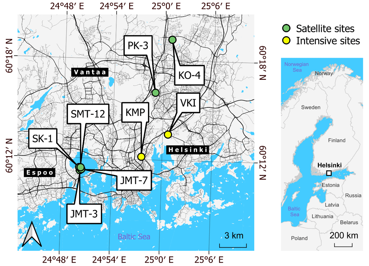
Figure 1 Locations of the intensive (yellow) and satellite (green) measurement sites around the Helsinki metropolitan area. There were two intensive sites in VKI (non-irrigated lawn and dry meadow) and two in KMP (irrigated lawn and mesic meadow). Satellite sites included two plots: a plot of lawn and a plot that was transformed from a lawn into a meadow during the campaign. Background maps were built with a topographic database by the National Land Survey of Finland (2023) and global administrative borders by GADM (2023).

2.1.2 Intensive sites

In order to study the CO₂ exchange with high temporal coverage and to compare the C balances of urban grasslands, two pairs of urban lawns and urban meadows, situated 4 km apart, were selected for the intensive measurement sites (Fig. 1, Table 1). In the neighbourhood of Kumpula (KMP), an old, mesic and mesotrophic urban meadow, which could be associated with “mesic perennial anthropogenic herbaceous vegetation (V39)” in the EUNIS classification (European Environment Agency, 2023) and hereinafter referred to as “mesic meadow”, was paired with a highly managed urban lawn, hereinafter referred to as “irrigated lawn”. Historically, the meadow was an old agricultural field on which farming practices were abandoned about 40 years ago. Currently, Aegopodium podagraria, Lupinus polyphyllus (non-native invasive), Dactylis glomerata, Anthriscus sylvestris, Elymus repens, Lamium album and Urtica dioica are the dominant plant species. It was cut once a year in autumn, and most of the vegetation clippings were taken away. It was neither irrigated nor fertilized. The lawn, mainly covered by Poa pratensis, was installed about 15 years ago. During the campaign, it was mowed automatically by a mowing robot that operated daily between 18:00 and 11:00 LT, and the grass clippings were pounded and left on the site. It was irrigated during the summer when needed and was last fertilized in spring 2021. The mesic meadow and the irrigated lawn were situated 150 m apart from each other. In the neighbourhood of Viikki (VKI), the urban lawn and urban meadow – hereinafter referred to as “non-irrigated lawn” and “dry meadow” – were situated inside a public park 60 m apart from each other. The urban lawn of Festuca sp. was sown in 2005 and managed as a “utility lawn” (Viherympäristöliitto, 2023). During the campaign, it was mown regularly so that the grass height was 4–12 cm, and the clippings were mostly left on the site. There was no irrigation, and the lawn had not been fertilized for several years. In 2020, a section of the park's lawns was transformed into a dry and nutrient-poor urban meadow by replacing the topsoil with a layer of recycled sand and sowing seeds. This young dry urban meadow tends toward a “dry perennial anthropogenic herbaceous vegetation (V38)” in the EUNIS classification (European Environment Agency, 2023). In 2022, the dominant species were Trifolium repens, Tripleurospermum inodorum, Leucanthemum vulgare, Centaurea jacea, Phleum pratense and Plantago major, and some rare species such as Dianthus deltoides, Campanula rotundifolia and Galium verum were also observed. It was fertilized in spring 2021 and mown for the first time in autumn 2022. After mowing, most of the clippings were removed from the site.

2.1.3 Satellite sites

To study the transformation process from an urban lawn into an urban meadow, six other sites belonging to local student housing associations were selected for high-spatial-coverage GHG measurements in the urban green space (Fig. 1, Table 1). Six urban lawns over 20 years old, each located near the developing urban meadows and all subject to regular lawn management, were selected and studied as control cases. All of the six lawns were predominantly covered by grasses (mostly Poa pratensis, Festuca rubra and Lolium perenne). In each of the sites, 50 m² of the already-established lawn was transformed into an urban meadow plot by volunteering and community participation. The transformations were conducted during late autumn 2020 by manually turning over the existent soil up to a depth of ca. 35 cm, followed by the sowing of 14 pollinator-friendly forbs at a density of 0.06 g m⁻². The commercial seed mixture (Suomen Niittysiemen Oy, Koski Tl, Finland) also included four grass species at a density up to 0.6 g m⁻². Consequently, the hemiparasitic forb Rhinanthus minor, which is known to have negative effects on grass cover (Chaudron et al., 2021), was sown at a 5 g m⁻² density. Every year since the lawn transformation, each of the developing urban meadows was managed by manually removing on-site tree seedlings (mainly Acer platanoides) before a one-time mowing event in autumn by hand scythe. Lastly, all mowing clippings were removed from the sites.

2.1.4 Sampling design

In this study, the lawn and the meadow within a pair were paired considering the short distance between each other, and the two plots were mostly visited on the same day. GHG flux measurements were conducted at each plot along a transect. All the data were collected at four fixed quadrats of approximately 1 m² distributed along a single transect. At the intensive sites, most of the quadrats were about 10 m apart, but to fit the study setup to the landscape design, there were some variations mainly due to passing walking paths: at the non-irrigated lawn, the quadrats were separated by 10, 5 and 10 m; at the dry meadow, the quadrats were separated by 17, 10 and 10 m; at the mesic meadow, the quadrats were located exactly 10 m apart; and lastly, the quadrats on the irrigated lawn were located in two separate transects 15 m away from each other, with the two quadrats on each transect being 3 m apart. At the satellite sites, from the centroid of the plot, a 10 m long transect was established along the length of the plot, with four quadrats of 1 m² area each uniformly distributed.

Soil temperature, soil moisture, soil samples and plant functional type cover percentages were collected close to the GHG measurement quadrats, except for the irrigated lawn, in which we used soil samples collected from the same plot by Ahongshangbam et al. (2023).

2.2 Flux measurements

2.2.1 Measurement protocol

The GHG flux measurements were conducted with manual chambers using different setups at the intensive and satellite sites. At the intensive sites, the carbon dioxide (CO₂) exchange measurements were conducted more frequently than at the satellite sites, and they also included the light response (LR) of net ecosystem exchange (NEE). At the satellite sites, the measurements also included methane (CH₄) and nitrous oxide (N₂O) exchanges, but measurements were conducted with opaque chambers, thus disabling photosynthesis. The chamber measurements were always performed within the above-mentioned quadrats.

At the intensive sites, the light response of NEE was measured fortnightly between June and September 2021–2022. Additional measurements of NEE, but mainly of total ecosystem respiration (TER), were also conducted in May and in October–November. Over the 2 years of measurements, the KMP lawn was visited 23 times, including 15 d of LR; the KMP meadow 23 times, including 16 d of LR; and the VKI lawn and meadow 20 times, including 15 d of LR, and at each site, most of the time the four collars were measured at a site (Table S2 in the Supplement). The measurement setup consisted of a transparent chamber attached to a CO₂ and H₂O analyser (Li-840A, LI-COR, Inc., Nebraska, USA), an air temperature and humidity sensor (BME280, Bosch Sensortec GmbH, Reutlingen, Germany), and a photosynthetically active radiation (PAR) sensor (PQS1, Kipp & Zonen, Delft, the Netherlands). The air was circulated through the analyser at a flow rate of 1 L min⁻¹, and the chamber was equipped with a small fan to ensure air mixing within the chamber headspace. We used two different sizes of chambers, either 0.072 or 0.288 m³, and three collars of different heights (18.3, 20.8 and 50 cm) to individually match the height of the chamber–collar combination to that of the vegetation we were measuring during each measurement day. The transparent chamber was placed on the ground while avoiding damaging the plants, and a tight seal was created by using sand-filled cloth bags as insulation. In meadows, when a collar was used, it was placed on the ground and sealed with the cloth bags, and the chamber was placed on top of the collar. The duration of each chamber closure was at least 2 min. To determine the light response of NEE, we repeated the measurement five times at each collar under different PAR intensities (i.e. 100 %, 60 %, 36 %, 21.6 % and 0 % of the prevailing sunlight level) created by shading the chamber with netted or opaque fabrics. We first measured without covering the chamber and then covered it with one to three layers of mesh cloth. Eventually, we measured the last recording with an opaque cover. There was a pause of at least 1 min in between the single light intensities to ventilate the chamber and to allow the plants some time to acclimatize to the changing light level. While conducting the measurements on the field, we allowed for ±10 % variation in the PAR level during a single closure.

At the satellite sites, GHG measurements were conducted with an opaque chamber monthly, between May–September 2021–2022. Additional background measurements were conducted in July, August and October 2020, before the lawn transformations took place. In total, the sites were visited 13 times: 3 times before transformation, including 2 times with CH₄ and N₂O measurements and 1 time with only CO₂, and 10 times after transformation, including 6 times with CH₄ and N₂O measurements and 4 times with only CO₂ (Table S2). A single measurement was performed at each of the four selected 1 m² quadrats at each plot (Table S2). To allow for a good representativity of CO₂ measurements, but also measurements of N₂O and CH₄, two different types of devices were used over the different months (Table S2). The measurement setup in August and October 2020, as well as in May, July and September 2021 and 2022, consisted of a CO₂, H₂O, N₂O and CH₄ analyser (DX4015, Gasmet Technologies Oy, Vantaa, Finland) connected to an opaque chamber equipped with a small fan. This Fourier transform infrared-based analyser was zero-calibrated at the beginning of each measurement day. The chamber volume was either 0.00456 or 0.268 m³ depending on the height of the vegetation measured. An additional collar of 20 cm height was needed to allow enough room for tall vegetation in July 2021 and 2022. The measurements in July 2020 and in June and August 2021 and 2022 were conducted with a setup consisting of an opaque chamber (volume 0.007434 m³) equipped with a CO₂ probe (GMP343, Vaisala Oyj, Vantaa, Finland), a relative humidity and air temperature sensor (HMP75, Vaisala), and a small fan. This chamber is introduced in detail by Ryhti et al. (2021). When measuring only CO₂ (i.e. July 2020, June and August 2021 and 2022), the duration of each chamber closure was 4–5 min. We extended the closure time to 15 min when measuring also N₂O and CH₄ (i.e. August and October 2020, May, July and September 2021 and 2022).

2.2.2 Flux calculation

The measurements represent the total ecosystem fluxes, i.e. the sum of inflow and outflow of CH₄ fluxes ($\mathrm{\mu }\mathrm{g}{\mathrm{CH}}_{\mathrm{4}}{\mathrm{m}}^{-\mathrm{2}}{\mathrm{s}}^{-\mathrm{1}}$), N₂O fluxes ($\mathrm{\mu }\mathrm{g}{\mathrm{N}}_{\mathrm{2}}\mathrm{O}{\mathrm{m}}^{-\mathrm{2}}{\mathrm{s}}^{-\mathrm{1}}$) and CO₂ fluxes (NEE, $\mathrm{\mu }\mathrm{g}{\mathrm{CO}}_{\mathrm{2}}{\mathrm{m}}^{-\mathrm{2}}{\mathrm{s}}^{-\mathrm{1}}$). NEE includes possible photosynthetic input (GPP, $\mathrm{\mu }\mathrm{g}{\mathrm{CO}}_{\mathrm{2}}{\mathrm{m}}^{-\mathrm{2}}{\mathrm{s}}^{-\mathrm{1}}$) and the outflow by respiration (TER, $\mathrm{\mu }\mathrm{g}{\mathrm{CO}}_{\mathrm{2}}{\mathrm{m}}^{-\mathrm{2}}{\mathrm{s}}^{-\mathrm{1}}$), which includes both autotrophic and heterotrophic respiration. This can be mathematically written as

$$\begin{array}{}\text{(1)}& \text{NEE}\left(t\right)=\text{TER}\left(t\right)+\text{GPP}\left(\text{PAR}\right(t\left)\right),\end{array}$$

where PAR ($\mathrm{\mu }\mathrm{mol}{\mathrm{m}}^{-\mathrm{2}}{\mathrm{s}}^{-\mathrm{1}}$) is photosynthetically active radiation and t is time. Here we used meteorological notation; i.e. we considered the inflow of carbon to be negative (GPP≤0), and therefore NEE could be either negative (i.e. sink of CO₂), when the absolute value of GPP was higher than TER, or positive (i.e. source), when TER was higher than the absolute value of GPP.

NEE or the total flux of other GHG fluxes during each chamber closure was calculated with the following (Eq. 2):

$$\begin{array}{}\text{(2)}& \text{flux}={\left({\displaystyle \frac{\mathrm{d}C\left(t\right)}{\mathrm{d}t}}\right)}_{t=\mathrm{0}}{\displaystyle \frac{M_{\text{GHG}}PV}{RTA}},\end{array}$$

where ${\left(\frac{\mathrm{d}C\left(t\right)}{\mathrm{d}t}\right)}_{t=\mathrm{0}}$ is the time derivative ($\mathrm{ppm}{\mathrm{s}}^{-\mathrm{1}}={\mathrm{10}}^{-\mathrm{6}}{\mathrm{s}}^{-\mathrm{1}}$) of the linear regression, M_GHG is the molecular mass of the GHG (44.01 g mol⁻¹ for CO₂, 16.05 g mol⁻¹ for CH₄ and 44.02 g mol⁻¹ for N₂O), P is the air pressure (Pa), V is the system (chamber and possible collar) volume (m³), R is the universal gas constant (8.31446 $\mathrm{J}{\mathrm{mol}}^{-\mathrm{1}}{\mathrm{K}}^{-\mathrm{1}}$), T is the temperature inside the chamber headspace during the closure (K) and A is the soil surface (i.e. the basal area of the chamber, m²).

TER, CH₄ and N₂O fluxes were obtained from the measurement conducted with the opaque cover (intensive sites) or with the opaque chamber (satellite sites).

To ensure proper air mixing inside the chamber, at least 10 s was removed from the beginning of each closure before fitting a linear regression into the GHG concentration values. Otherwise, the quality control and the length of the measurements included in the flux calculations differed between the instruments and GHGs. For the Vaisala equipment, CO₂ fluxes were calculated with the first minute of the recordings with R (version 4.2.2) after visual validation of linearity. Python (version 3.9.7) was used to calculate the fluxes measured by the two other devices (Vekuri, 2024). With the Gasmet analyser, the CO₂ fluxes were calculated from the first 5 min of the recordings, whereas CH₄ and N₂O fluxes, which were significantly lower fluxes and closer to the detection limits of the equipment, were calculated with the first 7 min of the recordings. For the intensive sites, where the LI-COR analyser was used, all fluxes were calculated from the first minute of the recording. There, possible poor-quality measurements were eliminated from the end of the measurement period if there was at least 1 min of good-quality data. The quality control measures were stability of light conditions inside the chamber during the closure and normalized root mean squared error (NRMSE) of the fit. Yet, it is worth noting that in cases where the flux is nearly zero, NRMSE can be very large even though the measurement is not erroneous. Therefore, we did not discard measurements based on NRMSE if $(\frac{\mathrm{d}C\left(t\right)}{\mathrm{d}t}{)}_{t=\mathrm{0}}$ was below 0.1 ppm s⁻¹. Otherwise, measurements were discarded if NRMSE was larger than 0.05. Accordingly, 41 NEE measurements out of 1225 recordings were discarded from the intensive site dataset, but none of them referred to the opaque chamber measurements, i.e. TER. Thus, TER was represented by 23 and 20 d of data at the KMP and VKI sites, respectively. Regarding the satellite sites, the filtering process described above was also applied to the Gasmet dataset, resulting in discarding 23 measurements of TER out of 384 recordings over the 3 years of measurements, but no CH₄ or N₂O measurements (384 recordings of each in total). All TER measurements (240 TER recordings in total) measured with the Vaisala device were considered to be valid (Table S2).

2.2.3 Light response (LR) fitting and daily GPP

In order to fit LR curves to the CO₂ flux data, we first subtracted TER from the other NEE rates to obtain an estimate for GPP (Eq. 1). GPP(PAR=0) was set to 0. The LR curve was expected to be a rectangular hyperbola (Ruimy et al., 1995) as follows:

$$\begin{array}{}\text{(3)}& \text{GPP}={\displaystyle \frac{\text{PAR}\mathit{\alpha }\mathit{\text{GPmax}}}{\text{PAR}\mathit{\alpha }+\mathit{\text{GPmax}}}},\end{array}$$

where PAR ($\mathrm{\mu }\mathrm{mol}{\mathrm{m}}^{-\mathrm{2}}{\mathrm{s}}^{-\mathrm{1}}$) is photosynthetically active radiation, α (mg µmol⁻¹) is the initial slope between GPP and PAR, and GPmax ($\mathrm{mg}{\mathrm{CO}}_{\mathrm{2}}{\mathrm{m}}^{-\mathrm{2}}{\mathrm{s}}^{-\mathrm{1}}$) is the light-saturated photosynthesis rate. The parameters α and GPmax were estimated using non-linear least-squares minimization. α was allowed to vary between −0.1 and $-\mathrm{1}\times {\mathrm{10}}^{-\mathrm{8}}$ mg µmol⁻¹ and GPmax between −5 and $-\mathrm{1}\times {\mathrm{10}}^{-\mathrm{7}}$ $\mathrm{mg}{\mathrm{CO}}_{\mathrm{2}}{\mathrm{m}}^{-\mathrm{2}}{\mathrm{s}}^{-\mathrm{1}}$.

In order to fit the LR curve for one collar, a minimum of three measurements done at different light intensities was required. After processing the light response calculation, LR curves where α had a standard error over 0.0008 mg µmol⁻¹ or where the GPmax standard error was higher than 10 $\mathrm{mg}{\mathrm{CO}}_{\mathrm{2}}{\mathrm{m}}^{-\mathrm{2}}{\mathrm{s}}^{-\mathrm{1}}$ were discarded from the dataset. In addition, LR was discarded if the highest PAR intensity in the response was under 500 $\mathrm{\mu }\mathrm{mol}{\mathrm{m}}^{-\mathrm{2}}{\mathrm{s}}^{-\mathrm{1}}$. That resulted in 154 LR curves out of 212, representing 14 d of data at the KMP meadow and VKI lawn and meadow and 10 d at the KMP lawn, which were used in further analyses.

Daily GPP was calculated for each collar and for each measurement day using Eq. (3), fitted parameters for the collar and day, and continuous PAR measurements from the SMEAR III station (Institute for Atmospheric and Earth System Research, 2023). First, GPP was estimated for each half hour with the fitted parameters and the 30 min average PAR. Then, all half-hourly GPPs were summed up to obtain the daily GPP of the collar on the particular day.

To compare the mean GPP at the different intensive sites, we selected consecutive weeks where all sites had a high number of high-quality LR curves. We estimated the mean daily GPP for all sites by utilizing the means of the obtained LR parameters at each site and the 30 min average PAR values over the 2 weeks. The 1-week periods that were included in this comparison started on 31 May, 14 and 28 June, 12 July, and 9 August in 2021 and on 16 May, 13 and 27 June, and 8 August in 2022.

2.3 Soil analyses

2.3.1 Soil temperature and soil moisture

Soil temperature and soil moisture were always measured together with the chamber measurements within the 1 m² quadrats at both the intensive and the satellite sites. One replicate of soil temperature was measured within the quadrats at a 10 cm depth with a handheld soil thermometer (HH376, Omega Engineering Inc., Connecticut, USA), and four to five replicates of soil moisture at 5 cm depth were measured with a handheld setup (ML3 ThetaProbe and HH2 Moisture Meter, Delta-T Devices Ltd., Cambridge, UK).

2.3.2 Soil characterization

At the intensive sites, overall soil characteristics, soil density, and C and N contents were analysed.

To determine the overall soil characteristics, we collected altogether 1 L of soil up to 25 cm depth at each of the sites or plots. At the irrigated lawn, the pooled sample comprised 16–18 individual samples collected in 2020 around the site with a thin auger (d=2.3 cm). At the rest of the remaining intensive sites, the samples were collected in 2021 with a slightly larger auger (d=5.0 cm) to collect four individual samples that were then pooled together. The fresh samples were stored in a fridge and sent to the lab within 1–3 d after collection. From these samples, particle size distribution (analysed according to Elonen, 1971) and the overall soil characteristics were analysed at a commercial laboratory (Eurofins Viljavuuspalvelu Oy, Mikkeli, Finland).

Soil density samples were collected by digging a small pit and carefully inserting a steel cylinder horizontally into an undisturbed pit wall at 10 cm depth. When the cylinder was fully inserted, it was gently detached by removing the surrounding soil while ensuring that all soil within the cylinder remained in place in order to achieve volumetric accuracy. Five replicates were collected at the KMP lawn and three replicates at the other intensive sites. After collection, the samples were dried at 105 ^∘C for 48 h, and the dry weights were weighed.

Other soil samples were collected to determine C and N contents. At KMP sites, samples for C and N were collected with a soil auger down to a 30 cm depth. Altogether, six individual samples were collected at the lawn and the meadow. At VKI, we used a soil auger to collect eight samples and then pooled them together. The irrigated lawn samples were first sieved with a 2 mm mesh sieve and then dried at 105 ^∘C for 24 h. At the other intensive sites, the samples were first dried at 105 ^∘C for 48 h and then sieved with a 2 mm mesh sieve. Total soil C and N contents were determined from the dried and milled samples of soil with a grain size smaller than 2 mm with an elemental CN analyser (LECO, Michigan, USA). The soil C and N contents were assumed to be only organic components without carbonates, i.e. soil organic carbon (SOC) and soil organic nitrogen (SON).

At the satellite sites, overall soil characteristics, soil C and N contents, and soil particle distribution were also determined. All soil samples from the satellite sites were collected in early July 2022, and all samples were extracted within the 1 m² quadrats. A total of four soil cores, dug using a soil auger down to ca. 15 cm depth, were pooled together to create a composite soil sample. In each of the plots, four composite soil samples were collected in ziplock bags and kept on ice during soil collection. All soil samples were then stored at −20 ^∘C, until they were shipped and analysed at a commercial lab (Eurofins Viljavuuspalvelu Oy, Mikkeli, Finland). Total soil C and N contents were assumed to be only organic components without carbonates, and SOC and SON were determined from freeze-dried and milled samples with an elemental CN analyser (LECO, Michigan, USA). For the case of soil particle size distribution, a fraction of each of the soil samples was repeatedly washed with a 30 % H₂O₂ solution to remove its organic matter content. The resulting soil samples were then dried out at 105 ^∘C for 48 h, before sieving (mesh size=0.6 mm) the final mineral soils. The sieved soil samples were then mixed with a sodium pyrophosphate solution (0.05 M), and their sand, silt and clay proportions were calculated by means of a laser diffraction particle size analyser (Beckman Coulter LS230, Beckman Coulter Inc., California, USA).

2.4 Vegetation inventory

Vegetation inventories to estimate plant functional type covers were conducted in all intensive and satellite sites on 27 June and 21 July 2022, respectively, according to the quadrat sampling method. In each of the quadrats (see Sect. 2.1.4), the cover of each plant species was estimated and classified in one of the following plant functional type categories: forb, grass, horsetail, legume, moss, sedge or tree, where forb includes all other families of flowering vascular plants, which do not belong to one of the already-listed categories. An average cover proportion was calculated from the four quadrats to estimate the overall proportion of each plant functional type at a plot.

All collars were also photographed from above on each measurement day to calculate the green cover percentage of the basal area within the chamber using Canopeo (Patrignani and Ochsner, 2015).

2.5 Ecosystem modelling

To derive annual estimates of NEE, TER and GPP, the intensive sites were simulated using JSBACH (Reick et al., 2013), which is the land component of the Max Planck Institute Earth system model (MPI-ESM) (Giorgetta et al., 2013). JSBACH is a process-based model and calculates the dynamic carbon cycle and key driving factors, including seasonal dynamics in leaf area, momentary CO₂ fluxes, evapotranspiration, soil moisture, litter production and soil carbon dynamics.

The model was driven with hourly data (2005–2022) of air temperature, precipitation, short-wave and long-wave radiation, relative humidity, and wind speed. The driver data were derived from observations from the Kumpula weather station ($\mathrm{60}{}^{\circ }{\mathrm{12}}^{\prime }{\mathrm{14.0}}^{\prime \prime }$ N, $\mathrm{24}{}^{\circ }{\mathrm{57}}^{\prime }{\mathrm{38.9}}^{\prime \prime }$ E) operated by the Finnish Meteorological Institute (Finnish Meteorological Institute, 2023b). The data were gap filled by observations from the nearby urban measurement station SMEAR III (Järvi et al., 2009). Hourly ERA5-Land data (Muñoz-Sabater et al., 2021) were used to fill a small number of remaining gaps.

The vegetation in JSBACH is represented by plant functional types (PFTs). Here, the model was set up for simulating only one PFT, C₃ grass, for each site. The Logistic Growth Phenology (LoGro-P) model (Böttcher et al., 2016) is used to describe the phenology in JSBACH, where the temporal development of the leaf area index (LAI) of grass depends on both temperature and soil moisture. The maximum LAI for each site (Table S3 in the Supplement) was set based on Sentinel-2 data (Nevalainen et al., 2022; Nevalainen, 2022), whereas the model simulated the seasonal LAI dynamics driven by temperature and precipitation. In addition, in the simulation of the mesic meadow, the shedding of the grass was activated 65 d after the growth started to better simulate the observed LAI.

According to the soil particle size distribution, the soil texture at all sites was sandy loam. The parameters describing the soil properties follow the recommendations by Hagemann and Stacke (2015). However, the volumetric field capacity and wilting point for each site were adjusted based on the soil moisture measurements (Table S3). The root depths of the lawns were assumed to be shallower than those of the meadows (Table S3).

The photosynthesis of C₃ plants in JSBACH is described by the model of Farquhar et al. (1980). The photosynthesis is calculated once to get the unstressed canopy conductance, which is then scaled based on the soil moisture in the root zone to get the canopy conductance and photosynthesis under water stress. The available water in the root zone depends on the field capacity, root depth and a scaling factor $f=(W-W_{\text{wilt}})/(W_{\text{crit}}-W_{\text{wilt}})$. The scaling factor is applied for relative soil moisture values between $W_{\text{crit}}=f_{\text{crit}}\cdot W_{\text{max}}$ and $W_{\text{wilt}}=f_{\text{wilt}}\cdot W_{\text{max}}$, where W_max is the maximum moisture content in the root zone. No water is available to the vegetation when the soil moisture reaches f_wilt×W_max. The factors f_crit and f_wilt are given in Table S3. Moreover, the daily GPP values were used to adjust the photosynthetic parameters to meet the observations at each intensive site.

The model was used to derive the annual average GPP, TER and NEE for the 2005–2022 period. The simulations were set up to represent habitats where the soil organic matter accumulates over time from the litter of standing vegetation. This was achieved by running a long spin-up period (thousands of years). As it is often the case in urban areas, the soils at the intensive sites had not been accumulated from the litter of the current vegetation, and therefore the soil carbon pools in the model are not equal to the ones present at the sites. Due to this, the simulations may not reproduce the observed TER but instead represent a more general situation for these habitats. However, we also performed additional simulations where the soil carbon pools were adjusted to meet the observed TER values in 2021 and 2022. The agreement between the simulated and observed carbon fluxes was evaluated by R² and RMSE.

2.6 Drought definition

Since drought can be defined as a deficit of precipitation and an increase in evaporation (Wang et al., 2021), we estimated the drought period at our intensive sites with the standardized precipitation-evapotranspiration index (SPEI). We calculated the drought period at a 14 d scale with the SPEI R package (Vicente-Serrano et al., 2010; Beguería et al., 2014). The Penman–Monteith equation (Monteith, 1965) was used to calculate the potential evapotranspiration (PET) with the FAO-56 method (Allen et al., 1998). The altitude was fixed at 10 m and the latitude at $\mathrm{60}{}^{\circ }{\mathrm{11}}^{\prime }$ N.

The minimum temperature, maximum temperature, wind speed, cloud amount, dew point temperature, relative humidity and air pressure, all collected at an hourly scale at the Kumpula meteorological station and averaged at a daily level, were downloaded from the Finnish Meteorological Database (Finnish Meteorological Institute, 2023a).

The drought periods were defined weekly with SPEI under −1.5, corresponding to the highest value describing a severe drought (Wang et al., 2021): a week with at least one daily SPEI value under −1.5 was considered a drought week.

2.7 Statistical analyses

2.7.1 Statistical analyses regarding drought stress

With the collected data, the resilience of the different grassland vegetation types to drought events was estimated. As resilience is the result of both components – resistance and recovery – we studied in this paper only the resistance, which was defined as “the magnitude of disturbance that a system can absorb before shifting from one state to another” (Capdevila et al., 2021).

Thus, to estimate the direct impact of drought on lawns and meadows, we chose to primarily compare the old mesic meadow (KMP meadow) and the non-irrigated lawn (VKI lawn), since both of these vegetation types were older than 15 years and non-irrigated. In addition, we also included the irrigated lawn (KMP lawn) in the comparison to see the effect of irrigation. The yearly summer means of TER, daily GPP, green cover, soil temperature and soil moisture were calculated for each site, by considering that the summer season starts in week number 22 and ends in week number 34 (data collected from 31 May–24 August 2021 and 3 June–25 August 2022). Lastly, we calculated the differences between the measured values of the variable and the summer average of the same variable at the site level. These calculated differences were then normalized at a site and year level by subtracting the annual means of the differences and dividing the whole by the annual standard deviation of the differences.

With the summer data, we defined two categories: data collected during the drought events and data collected outside of the drought events. Finally, with the Mann–Whitney U tests, we compared, pair by pair, the VKI lawn, KMP lawn and KMP meadow in the different summer conditions.

2.7.2 Dynamics of GHG fluxes at the satellite sites

Considering the transformation from lawns into meadows at the satellite sites, Shapiro–Wilk tests were used to evaluate the normal distribution of each variable (i.e. CO₂ fluxes, CH₄ fluxes, NO₂ fluxes, soil moisture and soil temperature) by year and treatment (meadow vs. lawn). Then, differences in given variables between lawns and meadows were assessed either by t tests or Mann–Whitney U tests depending on the normality of the data.

2.7.3 Statistical analyses regarding plant functional types

The effects of plant functional types on SOC, SON and GHG fluxes were studied in all intensive sites and satellite plots with the vegetation and flux data collected in 2022. The fluxes were averaged for the growing season, from May to September. First, Mann–Whitney U tests were used to compare the proportions of grasses, legumes and forbs between lawns and meadows.

Then, the effects of vegetation functional types were assessed by applying linear mixed-effect models (LMMs), using the R lme4 package (Bates et al., 2015), where a factor describing the locations of the pair of a lawn and a meadow (Fig. 1) was included as a random effect. This factor was introduced to consider the spatial variability between the sites, as the environmental conditions of the lawn and meadow within each site were considered to be similar. If predictive variables, i.e. plant functional types, correlated over 0.70, one of the correlated plant functional types was discarded from the LMM according to the lowest cover proportion and the lowest occurrence in the dataset. Next, the normal distribution of each regression's residuals was visually checked with quantile–quantile (Q–Q) plots. In total, six mixed-effect multiple regressions, including the proportions of the selected plant functional types as predictive variables, were run by applying a backward selection. At each iteration, predictive variables with p values higher than 0.1 were removed, and variables with p values lower than 0.05 were considered to be statistically significant. P values were adjusted by a Kenward–Roger approach (Kenward and Roger, 1997) from the R lmerTest package (Kuznetsova et al., 2017), and a conditional R² was used to assess the quality of the model.

3 Results

3.1 Drought occurrences

There was 7 % and 12 % more precipitation in 2021 and 2022 compared to the 653 mm value of the 1991–2020 reference period (Jokinen et al., 2021), but in both years July was drier than the long-term average, with 17 % and 15 % less precipitation in 2021 and 2022, respectively (47 mm in 2021 and 49 mm in 2022 compared to 57 mm in 1991–2020). At the same time, 2021 and 2022 were 0.1 and 0.4 ^∘C warmer than the reference, which was 6.5 ^∘C. The summers were on average hotter than the reference period, with 2.5 and 1.8 ^∘C higher temperatures in 2021 and 2022, respectively, compared to 16.6 ^∘C. These particularly hot and dry weeks were observed from 14 June to 1 August 2021 and from 6 June to 17 July 2022 (Fig. 2a).

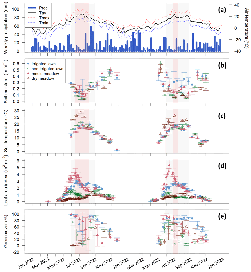
Figure 2 (a) Weekly precipitation (Prec.) and mean air temperature (T_av) recorded by the FMI meteorology station, (b) manually measured soil moisture at a 5 cm depth, (c) manually measured soil temperature at a 10 cm depth, (d) leaf area index from the Sentinel-2 satellite, and (e) manually measured green cover at the intensive study sites with standard deviations calculated for each site at a daily scale. The irrigated lawn is the KMP lawn, the non-irrigated lawn is the VKI lawn, the mesic meadow is the KMP meadow, and the dry meadow is the VKI meadow. The red rectangles indicate the drought periods according to the SPEI, and the light grey rectangles represent the summer season. In panel (a), T_max and T_min represent the weekly instantaneous maximum and minimum mean temperatures.

At the intensive sites, the measured soil moisture (Fig. 2b) also showed a drastic decrease at all sites during these two periods, except at the irrigated lawn (KMP lawn), where the soil moisture remained relatively high during the whole summer. The highest soil temperature was also reached during the same period (Fig. 2c). In 2021 and 2022, those hot and dry weeks also corresponded to the decrease phase of LAI, except at the dry meadow (VKI meadow), where LAI increased slowly from spring until August (Fig. 2d). The measured green cover notably followed the same patterns as the satellite LAI data (Fig. 2e).

Using SPEI, two drought periods were defined: the first one from 14 June to 8 August in 2021 and the second one from 27 June to 17 July in 2022 (Fig. 2). Thus, the defined drought event in 2021 happened early in the summer season and lasted 8 weeks, whereas the drought event in 2022 arrived later in the summer and lasted only 3 weeks. These two drought events co-occurred with the high-temperature and low-soil-moisture periods described above.

3.2 CO₂ fluxes

3.2.1 Observed seasonal variation

At all intensive sites, the measured TER increased at the beginning of the measurement campaign and declined during the drought events at the non-irrigated sites (Figs. 3 and S1 in the Supplement). When comparing the differences between the four sites, the mean momentary TER was the highest at the mesic meadow (KMP meadow, 0.44 and 0.31 $\mathrm{mg}{\mathrm{CO}}_{\mathrm{2}}{\mathrm{m}}^{-\mathrm{2}}{\mathrm{s}}^{-\mathrm{1}}$ in 2021 and 2022, respectively) and the lowest at the dry meadow (0.29 and 0.26 $\mathrm{mg}{\mathrm{CO}}_{\mathrm{2}}{\mathrm{m}}^{-\mathrm{2}}{\mathrm{s}}^{-\mathrm{1}}$ in 2021 and 2022, respectively). In 2021, the highest recorded mean values (0.86, 0.84, 0.59, 0.59 $\mathrm{mg}{\mathrm{CO}}_{\mathrm{2}}{\mathrm{m}}^{-\mathrm{2}}{\mathrm{s}}^{-\mathrm{1}}$) were measured at the non-irrigated lawn (VKI lawn), mesic meadow, dry meadow and irrigated lawn on 7 June, 2 July, 19 July and 11 August, respectively. In 2022, the highest values (0.71, 0.49, 0.65, 0.55 $\mathrm{mg}{\mathrm{CO}}_{\mathrm{2}}{\mathrm{m}}^{-\mathrm{2}}{\mathrm{s}}^{-\mathrm{1}}$) were recorded at the dry meadow, irrigated lawn, mesic meadow and non-irrigated lawn on 23 June, 30 June, 1 July and 17 August, respectively. In general, daily TERs were higher at KMP sites (irrigated lawn and mesic meadow) compared with VKI sites (non-irrigated lawn and dry meadow), although the highest values were not reached in a specific order.

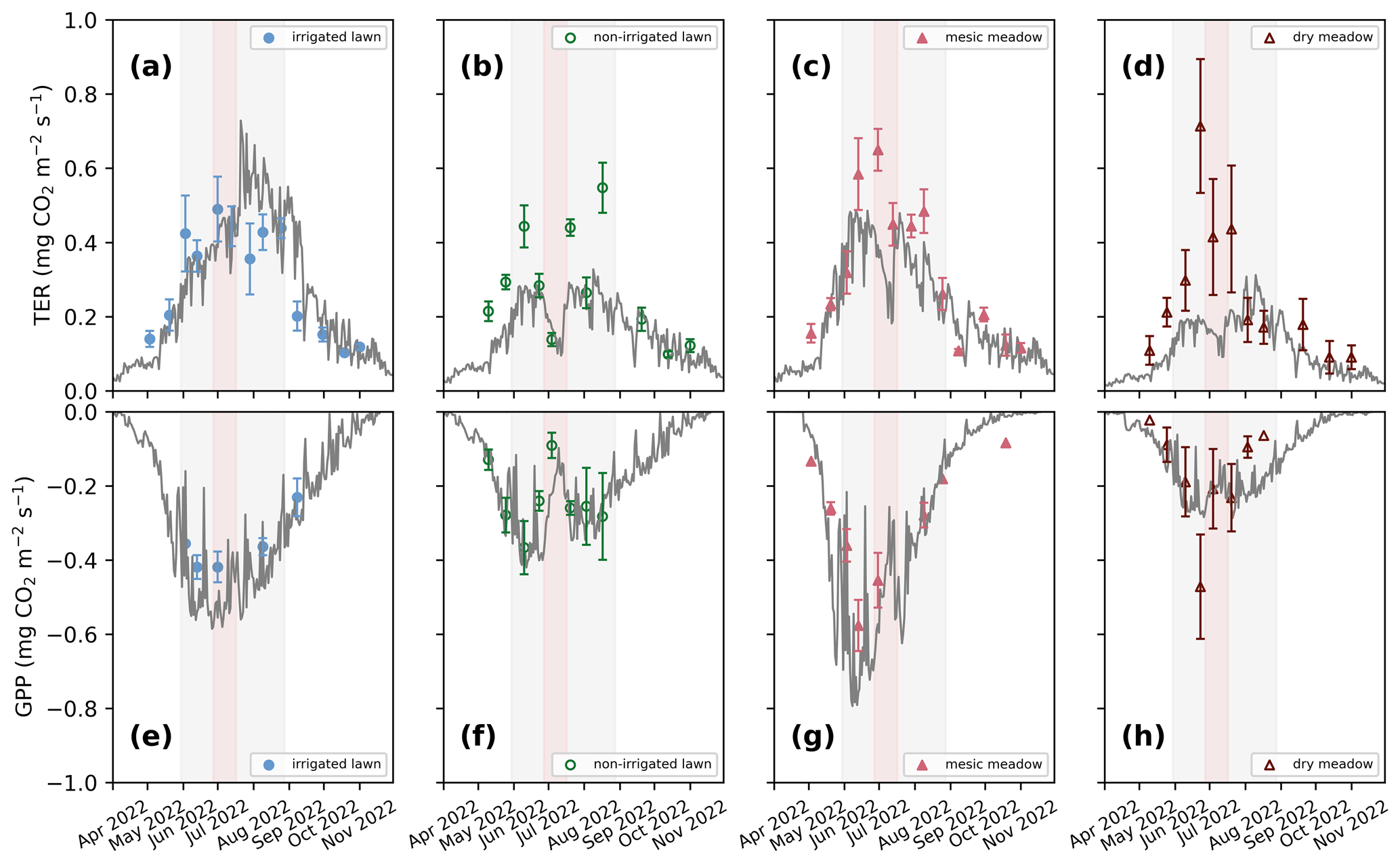
Figure 3 Seasonal dynamics of mean total ecosystem respiration (TER; a–d) and daily photosynthesis (GPP; e–h) in the four intensive sites in 2022. The continuous grey lines represent the JSBACH simulations, and the triangles and dots represent the mean of manual measurements with standard deviation bars. (a, e) Irrigated lawn: KMP lawn, (b, f) non-irrigated lawn: VKI lawn, (c, g) mesic meadow: KMP meadow, (d, h) dry meadow: VKI meadow. The red rectangles indicate the drought periods according to SPEI, and the light grey rectangles represent the summer season. The model simulated the whole year, but for clarity, January–March and December are not visible as there were no measurements during those months.

There were site-specific variations in the seasonal pattern of GPP (Fig. S1). In the first campaign year, after the first measurements, the daily GPP sink decreased at all sites except at the dry meadow, for which it was the first growing season after establishment. In 2022, the daily GPP sinks first increased and then started to decrease around the end of June (Fig. 3). In 2021, the highest recorded daily uptakes (−0.48, −0.51, −0.40, −0.46 $\mathrm{mg}{\mathrm{CO}}_{\mathrm{2}}{\mathrm{m}}^{-\mathrm{2}}{\mathrm{s}}^{-\mathrm{1}}$) were measured at the non-irrigated lawn, mesic meadow, dry meadow and irrigated lawn on 7 June, 18 June, 5 August and 11 August, respectively. In 2022, the order had also changed slightly as the daily highest uptakes (−0.37, −0.58, −0.42 and −0.47 $\mathrm{mg}{\mathrm{CO}}_{\mathrm{2}}{\mathrm{m}}^{-\mathrm{2}}{\mathrm{s}}^{-\mathrm{1}}$) were recorded at the non-irrigated lawn, mesic meadow, irrigated lawn and dry meadow on 10 June, 13 June, 13 June and 23 June. Thus, the measured GPP values were higher at KMP sites (irrigated lawn and mesic meadow) than at VKI sites (non-irrigated lawn and dry meadow).

The mean daily GPP rates during May–August 2021–2022 were −24.4, −16.7, −23.9 and −8.7 $\mathrm{g}{\mathrm{CO}}_{\mathrm{2}}{\mathrm{m}}^{-\mathrm{2}}{\mathrm{d}}^{-\mathrm{1}}$ at the irrigated lawn, non-irrigated lawn, mesic meadow and dry meadow, respectively, when comparing only the consecutive weeks that included high-quality measurements at all sites. The mean observed respiration rates were 0.39, 0.40, 0.51 and 0.35 $\mathrm{mg}{\mathrm{CO}}_{\mathrm{2}}{\mathrm{m}}^{-\mathrm{2}}{\mathrm{s}}^{-\mathrm{1}}$, respectively, during the same months.

3.2.2 JSBACH performance

In order to represent the average fluxes of the different habitats, the model was primarily initialized to reach a steady state with each vegetation type, and therefore the simulated soil carbon pool represents the result of long-term carbon input of the site itself. The simulated soil moisture (Fig. S2 in the Supplement) varied according to irrigation, precipitation and evaporation and showed lower values in summer, particularly in June and July, and also in August in 2022. The modelled seasonal dynamics in soil moisture followed the observations in general; however, some of the observations were considered to represent moisture content above the volumetric field capacity. The maximum soil moisture in the model is limited by the field capacity (Fig. S2). At the same time, the modelled soil temperature between 10 and 15 cm depth agreed with the measured soil temperature at 10 cm depth (Fig. S3 in the Supplement). Modelled LAI varied in accordance with the observations, especially at the mesic meadow and in the second year at the dry meadow (Fig. S4 in the Supplement). The dry meadow was established very recently and was found to be sparse and inhomogeneous with respect to the vegetation, and therefore the drought response was challenging to capture in the model simulation, particularly in 2021. The drought response for the non-irrigated lawn agreed with the observations in 2021, while in 2022 the recovery was too strong in the simulation. At the irrigated lawn, the simulated LAI decreased later in 2022 than the observed LAI (Fig. S4).

Simulated TER followed the dynamics in the observed seasonal cycle and, for example, showed a similar response to the 2022 drought but generally underestimated the overall level of the non-irrigated lawn and the dry meadow. The drought response was stronger in the mesic and dry meadow (Figs. 3e–h and S5e–h in the Supplement). For the irrigated lawn the benefits of irrigation may have been overestimated, seen as a weaker drought response in the model than in the observations. The irrigation used in the model was estimated as an average over the whole area, while there probably was less irrigation where the measurement equipment was installed. The highest R² values for TER were observed at the irrigated lawn and mesic meadow and the lowest at the dry meadow (Table 2). Adjusting the carbon pools to fit closer to observed TER values in 2021 and 2022 (Figs. S6 and S7 in the Supplement) mainly decreased RMSE but did not notably improve R² values at the different vegetation types in 2021 and 2022 (Table 2).

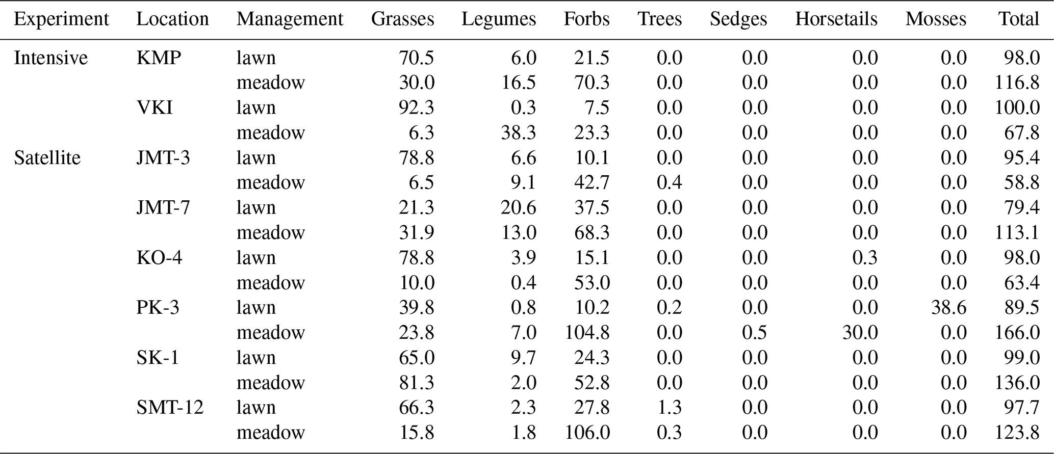
Table 1 Characteristics at the intensive sites and satellite plots including soil organic carbon (SOC), soil organic nitrogen (SON), and the ratio between SOC and SON (CN ratio) (± standard deviation), calculated for at least four replicates. At each VKI site there was only one replicate for each variable. Sown mixture indicates seeds of pollinator-friendly forbs, grass species and Rhinanthus minor, which were sown in late 2020, and veg. refers to vegetation. The particle distribution was originally determined for Finnish classification, and therefore, approximations were made for sand (0.06–2.0 mm), silt (0.002–0.06 mm) and clay (<0.002 mm).

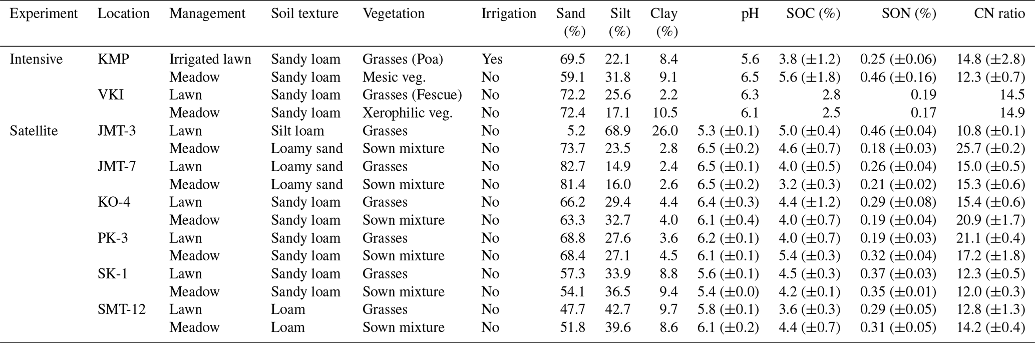
Table 2 R² and root mean square error (RMSE; $\mathrm{mg}{\mathrm{CO}}_{\mathrm{2}}{\mathrm{m}}^{-\mathrm{2}}{\mathrm{s}}^{-\mathrm{1}}$) calculated for total ecosystem respiration (TER) and gross primary production (GPP) in the standard simulation where the soil carbon was stabilized based on the standing vegetation and for the adjusted simulations (adj soil C) where the soil carbon pool was set so that simulated TER met the observations in 2021 and 2022.

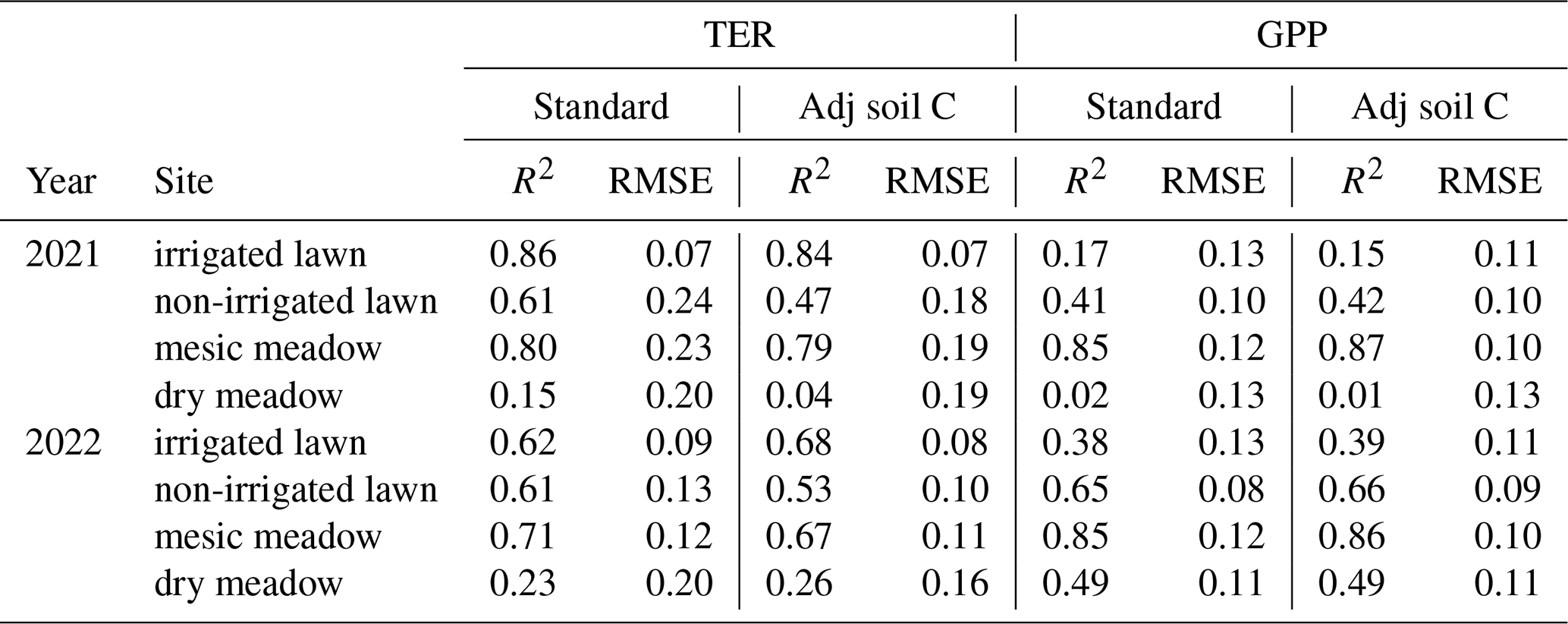
The model was able to simulate the overall level and the seasonal cycle in GPP at the irrigated lawn, non-irrigated lawn and mesic meadow (Figs. 3a–c and S5a–c, Table S5 in the Supplement). At the dry meadow, the model overestimated the increase in GPP in the early season during its first growing season in 2021 (Fig. S5d). The vegetation cover in the newly established meadow was very low in the early growing season in 2021, which was not accounted for in the model. The agreement was better in the following year (Fig. 3d, Table S5). The benefit of irrigation was also somewhat overestimated for GPP during the dry periods. Simulated daily mean GPP followed the observations closely for the non-irrigated lawn and mesic meadow (R² between 0.41 and 0.85, Table 2), while the dry meadow was difficult to simulate, especially in 2021 (Table 2, Fig. S5).

3.2.3 Annual balances

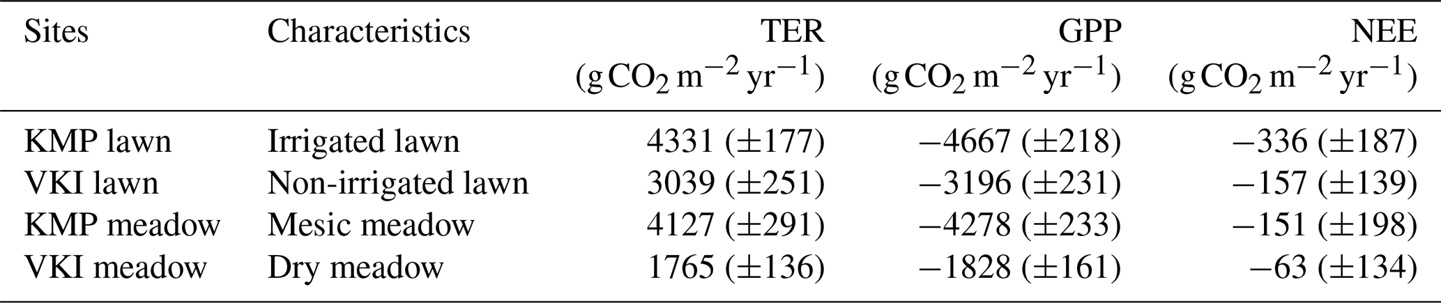
During 2005–2021, simulated annual GPP and TER were on average the highest at the irrigated lawn and mesic meadow (Table 3). GPP and TER were the lowest in the dry meadow (Table 3), being approximately 40 % of those of the irrigated lawn and meadow. The non-irrigated lawn's GPP and TER were approximately 70 % of those of the irrigated lawn. The lawns had, on average, more negative NEE, i.e. a greater sink of carbon than meadows, and looking at the ratio between standard deviation and NEE, meadows showed higher year-to-year variations than the lawns (Table 3). The sink of the irrigated lawn was approximately 53 % higher than that of the non-irrigated lawn (VKI lawn). Additionally, it was found that 13 %–16 % of TER occurred between November and March.

Table 3 Mean annual (± standard deviation) ecosystem respiration (TER), photosynthetic uptake (GPP) and net ecosystem exchange (NEE) modelled with JSBACH at the four intensive sites during the years 2005–2022.

According to the simulations that were adjusted to meet the TER observations, annual NEEs were 328, 2663, 1476 and 2140 $\mathrm{g}{\mathrm{CO}}_{\mathrm{2}}{\mathrm{m}}^{-\mathrm{2}}{\mathrm{yr}}^{-\mathrm{1}}$ in 2021 and −195, 1496, 571 and 1205 $\mathrm{g}{\mathrm{CO}}_{\mathrm{2}}{\mathrm{m}}^{-\mathrm{2}}{\mathrm{yr}}^{-\mathrm{1}}$ in 2022 at the irrigated lawn, the non-irrigated lawn, the mesic meadow and the dry meadow, respectively (Table S4 in the Supplement).

3.3 Extreme weather resistance

Green cover, TER and daily GPP were significantly decreased at the non-irrigated lawn compared to the records outside the drought and to the mature mesic meadow and the irrigated lawn during the prolonged drought in 2021 (Fig. 4a, c and e) and during the shorter drought in 2022 (Fig. 4b, d and f). In 2022, TER was significantly higher at the irrigated lawn and the mesic meadow during the drought than outside of the drought period (Fig. 4d).

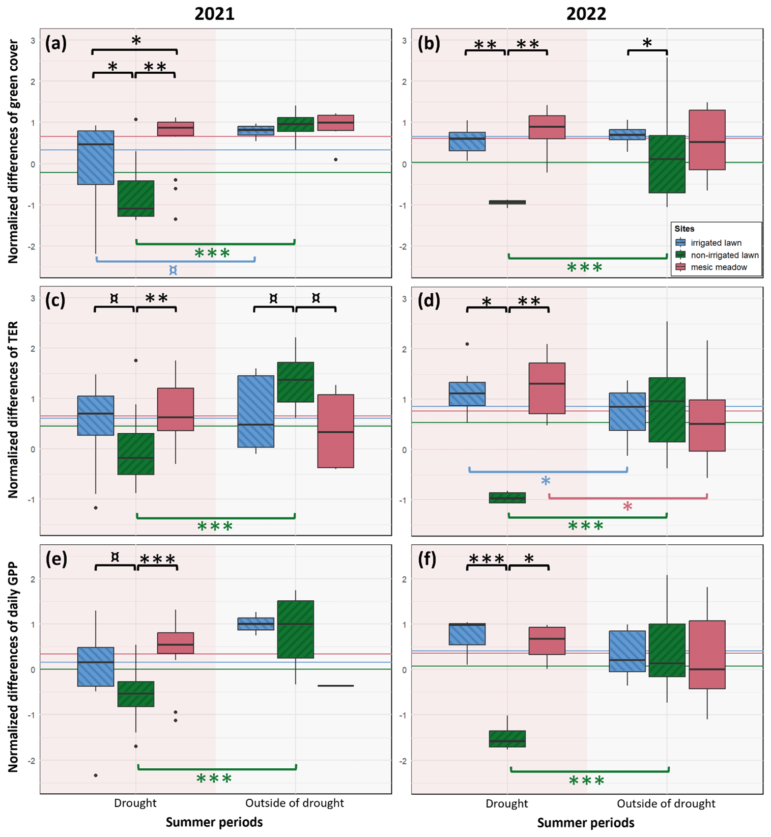
Figure 4 The resistance indices of an irrigated lawn (KMP lawn), a non-irrigated lawn (VKI lawn) and an old mesic urban meadow (KMP meadow) to drought events in 2021 (first column) and 2022 (second column), calculated for the green cover (a, b), the TER (c, d) and the daily GPP converted to positive values (e, f). The values are the differences between the measured values and the summer average, normalized at a yearly level. The horizontal lines represent the normalized summer means of each site. Summer includes June–August, and droughts were defined in Fig. 2 (14 June–8 August 2021 and 27 June–17 July 2022) (^¤, p value≤0.10; ^∗, p value≤0.05; ${}^{\ast \ast }$, p value≤0.01; ${}^{\ast \ast \ast }$, p value≤0.001).

3.4 CH₄ and N₂O fluxes

The measurements at the control lawn and transformed meadow of each site were conducted consecutively during the same day, and therefore the environmental conditions were as similar as possible. Indeed, soil moisture and temperature did not differ between the treatments during the measurements (Fig. S9 in the Supplement). At the satellite sites, before the transformation in 2020, there were no differences between lawns and meadows in terms of TER, CH₄ and N₂O fluxes measured in darkened conditions (Fig. 5). There was some general year-to-year variation in the median and range of observed CO₂ and CH₄ fluxes, but the fluxes did not differ between lawns and transformed meadows in 2021 or 2022 (p>0.1, Fig. 5a and b). The mean N₂O fluxes were slightly lower in meadows than in lawns in 2021 and 2022 (p value<0.1, Fig. 5c).

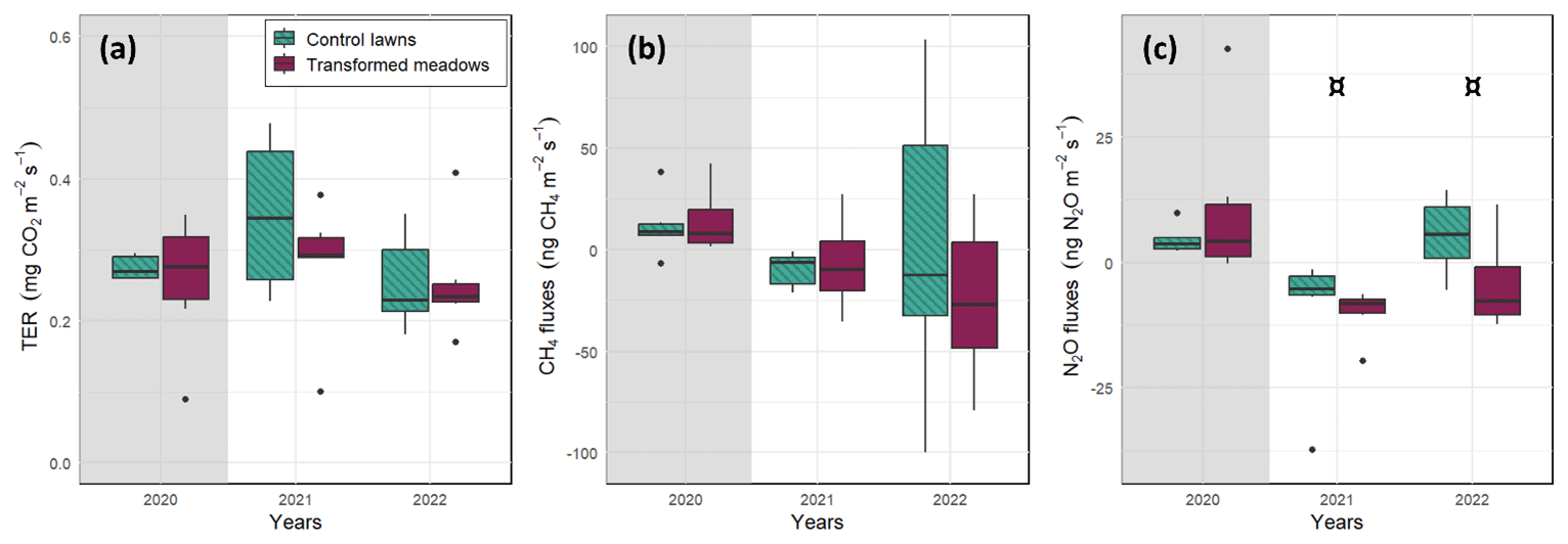
Figure 5 Box and whisker plots of measured (a) total ecosystem respiration (TER) and (b) CH₄ and (c) N₂O fluxes of lawns and transformed meadows at the satellite sites before (grey background) and after (white background) transformation, which happened at the end of 2020 only at the transformed meadows. The environmental conditions were considered to be similar between the two treatments. Statistical differences between the treatments were tested at the year level (^¤, p value≤0.10; ^∗, p value≤0.05).

3.5 Plant functional type predictor variables for C and N cycles

On average, the total vegetated area of the studied meadows (Table 4) did not significantly differ from that on lawns (U=40.000, p value=0.442), but the cover proportions of the main plant functional types shared by both vegetation types differed. Meadows had a significantly lower proportion of grass cover (i.e. 25 %) than lawns (65 %, U=10.000, p value=0.002). Most of the meadow area was covered by forbs other than legumes (i.e. 65 %), a proportion significantly larger (U=16.000, p value=0.002) than that found in lawns (i.e. 19 %). Nevertheless, the proportion of legume cover was found to be statistically similar (U=39 000, p value=0.505) in meadows (11 %) and lawns (6 %).

Table 4 Cover proportions (%) of the different plant functional types: grasses (Poaceae), legumes (Fabaceae), forbs (other families of flowering vascular plants, which do not belong to one of the listed categories), trees, sedges (Carex), horsetails (Equisetum) and mosses (Bryophyta), inventoried on 27 June and 21 July 2022. The total column is the sum of all the plant functional type covers; a fully covered quadrat with only one layer of vegetation should have a 100 % cover, >100 % indicates layered vegetation (short and tall grassland plants) and <100 % indicates the presence of bare soil. See locations in Fig. 1.

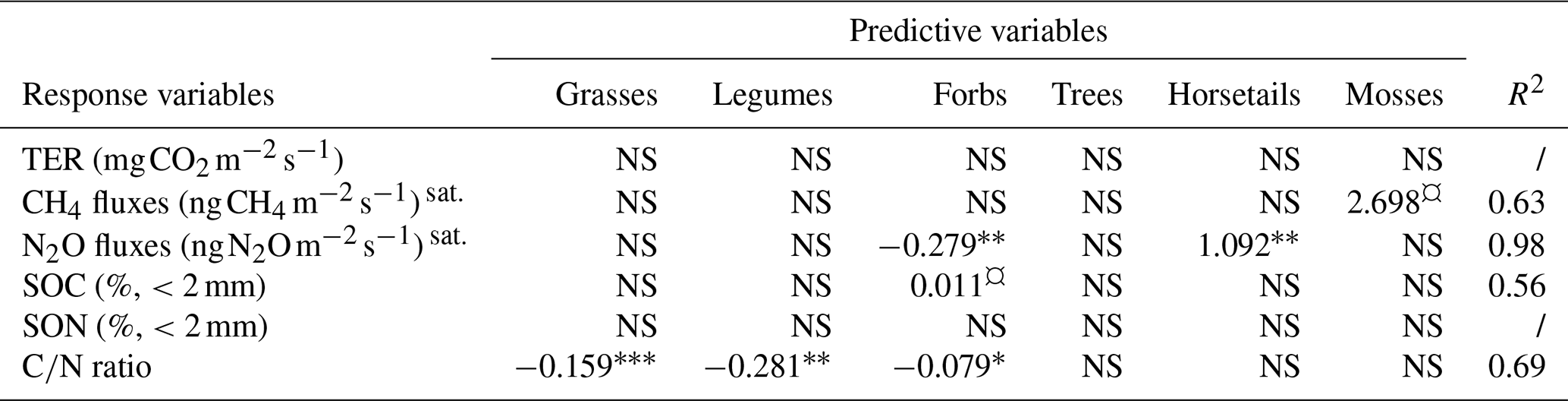
Next, we explored possible correlations between cover proportions of common plant functional types and variables related to C and N cycles. First, we discarded sedges from the analysis since their cover proportion was correlated with that of horsetails (>0.7, Table S7 in the Supplement) and were only present at one plot and in a low proportion (Table 3). The cover proportions of none of the functional plant types are significantly associated with either TER or SON. Yet, the CH₄ flux appeared to be positively associated with moss cover (Table 5). Additionally, the N₂O flux was significantly negatively associated with forb cover and positively associated with horsetail cover proportion (Table 5). SOC was slightly positively explained by forb cover proportion (Table 5). The $\mathrm{C}/\mathrm{N}$ ratio was significantly negatively associated with legume, grass and forb cover proportions (Table 5).

Table 5 The connection between the cover proportions (%) of different plant functional types and total ecosystem respiration of CO₂ (TER), CH₄ fluxes, N₂O fluxes, soil C content (SOC), soil N content (SON) and $\mathrm{C}/\mathrm{N}$ ratio. The plant functional types are grasses (Poaceae), legumes (Fabaceae), forbs (other families of flowering vascular plants, which do not belong to one of the listed categories), trees, sedges (Carex), horsetails (Equisetum), and mosses (Bryophyta) (NS, p value>0.10; ^¤, p value≤0.10; ^∗, p value≤0.05; ${}^{\ast \ast }$, p value≤0.01; ${}^{\ast \ast \ast }$, p value≤0.001). ^sat. indicates values that were only measured at satellite sites.

4 Discussion

It is well known that converting lawns into meadows can increase the presence of different plants and arthropods in cities (Venn and Kotze, 2014; Wastian et al., 2016; Chollet et al., 2018). In this study, we wanted to better understand how transforming lawns into meadows in Nordic urban areas could affect their GHG fluxes and how varying cover proportions of their different plant functional types could influence the C and N cycles of these green spaces. The studied sites, an irrigated lawn, a non-irrigated lawn, an old mesic spontaneous meadow and a young dry meadow, were mainly C sinks. Moreover, with a focus on the transformation dynamic from lawns into meadows, no significant differences in measured GHG fluxes (i.e. CO₂, CH₄ and N₂O) were found between the six control lawns and six transformed meadows in the 2 years following the conversion. However, the studied mesic meadow appeared to be more resistant to drought stress than an non-irrigated lawn. This resistance could notably be explained by a shift in vegetation functional types and a less homogeneous vegetation setting, as discussed later. Furthermore, as expected, the cover proportion of forbs was found to be higher in meadows than in lawns and seems to be negatively associated with N₂O fluxes and $\mathrm{C}/\mathrm{N}$ ratio and positively associated with SOC of the green space.

4.1 Fluxes in urban grasslands

Carbon neutrality, or even a net positive scenario, is nowadays one of the major goals for cities and states in mitigating climate change (Lwasa et al., 2022). Our aim was to understand how CO₂ sequestration differs between lawns and meadows by studying contrasting vegetation types, a mesic mesotrophic meadow and a dry nutrient-poor meadow, together with irrigated and non-irrigated lawns to determine the full range of their GHG exchange. We found that the photosynthetic production (GPP) of an irrigated lawn and a mesic meadow was roughly equal on a mean daily and an annual scale, whereas the GPP of a non-irrigated lawn was notably lower. At an annual level, irrigation increased the GPP of a lawn by over 40 % and the sink (NEE) by more than 100 %. It has already been found that water input improves carbon uptakes (Thienelt and Anderson, 2021) and demonstrated by Zirkle et al. (2011) that irrigated lawns store up to 10 $\mathrm{g}\mathrm{C}{\mathrm{m}}^{-\mathrm{2}}{\mathrm{yr}}^{-\mathrm{1}}$ more carbon in soil than non-irrigated ones. Also, our analysis of annual NEE indicated that an irrigated lawn is a stronger sink, approximately 50 $\mathrm{g}\mathrm{C}{\mathrm{m}}^{-\mathrm{2}}{\mathrm{yr}}^{-\mathrm{1}}$ higher than a non-irrigated lawn. Here, the model estimates for NEE were uncertain as the model was unable to simulate some of the observed momentary total ecosystem respiration (TER) values during summertime (Fig. 3), which caused the full carbon balance estimate to be more uncertain than the estimated GPP. The uncertainty in the annual TER and NEE estimate is further highlighted by the mean observed TER between May and August, where the order of the sites differed from the one in simulated annual TER values. However, the momentary TER varies, based especially on soil moisture, temperature and autotrophic activity (Ryan and Law, 2005; Subke et al., 2006; Mäki et al., 2022), therefore making a mean without standardizing the environmental conditions might be inaccurate, as the momentary measurements at the satellite sites were collected during different times, i.e. environmental conditions.

In this experiment, we measured the collars at various times of the day for practical reasons, even though Pavelka et al. (2018) suggest measuring ecosystem respiration in the morning around 09:00–10:00 LT to get the average level of daily respiration. Moreover, with manual chamber measurements, we were able to measure only once or twice a month and most of the time under sunny weather conditions, whereas with automatic chambers or eddy covariance (Hiller et al., 2011; Thienelt and Anderson, 2021), it would have been possible to estimate the daily and monthly variations at a finer scale and to reduce the bias caused by hot and dry days. Therefore, especially during the summertime, the measured values most probably are overestimations of the daily average, whereas in the early spring and in autumn, when plants are less active and the diurnal amplitude in soil temperature is smaller, the observations fit the model estimate closely. Decina et al. (2016) found that during the growing season, TER was about 0.198 ± 0.006 $\mathrm{mg}{\mathrm{CO}}_{\mathrm{2}}{\mathrm{m}}^{-\mathrm{2}}{\mathrm{s}}^{-\mathrm{1}}$ at urban lawns in Boston, USA, which is lower than the values measured at our plots. Lastly, it has been shown that during cold days, under snow and/or frozen ground, grasslands are a source of CO₂ (Hiller et al., 2011; Jasek-Kamińska et al., 2020). The model was also run for winter months, with the heterotrophic soil respiration decreasing at the same time as the soil temperature until reaching a minimum in late winter. Although the highest ecosystem activities and emissions take place in the warm summer months, to fully validate the annual balance, it would be useful to have some additional wintertime observations. Nevertheless, we can be quite confident in the simulated photosynthetic production, since GPP principally occurs during the snow-free seasons.

Furthermore, soil respiration is highly related to soil carbon quality and quantity (Davidson and Janssens, 2006). Here, it seems evident that the studied soil was not stabilized but, rather, that growing media with unknown properties were either brought to the site or some earlier vegetation type built the soil carbon storage. This is most distinct in the young sites (less than 15 years old) and most managed sites, i.e. the lawns and the dry meadow. It highlights unpredictable features of urban soils, which are characterized by high anthropogenic disturbances, unknown origins and changes in land use. Thus, the quality and quantity of organic matter cannot be connected to a linear history even at a city scale (Pouyat et al., 2006; Setälä et al., 2016; Ivashchenko et al., 2019; Sushko et al., 2019; Cambou et al., 2021). Here, we chose to estimate the carbon balance over an extended time in stabilized conditions, and all our sites were estimated to be small sinks of carbon varying between 63–336 $\mathrm{g}{\mathrm{CO}}_{\mathrm{2}}{\mathrm{m}}^{-\mathrm{2}}{\mathrm{yr}}^{-\mathrm{1}}$. However, adjusting the model parameters to reproduce values closer to the observed TER values turned most of the sites into sources of atmospheric CO₂ during the measurement years of 2021 and 2022. Even if those values represent the current situation at the study sites, they also represent a destabilized state, whereas the extended runs stand for long-term carbon balances of these vegetation types.

Many studies have reported urban grasslands to be C sources at least in certain conditions (Allaire et al., 2008; Hiller et al., 2011; Bezyk et al., 2018), but some have also reported sinks of about 20–180 $\mathrm{g}{\mathrm{CO}}_{\mathrm{2}}{\mathrm{m}}^{-\mathrm{2}}{\mathrm{yr}}^{-\mathrm{1}}$ (Thienelt and Anderson, 2021). However, most studies focus on the respiration rate, omitting GPP (Kaye et al., 2005; Decina et al., 2016; Lerman and Contosta, 2019; Sushko et al., 2019; Upadhyay et al., 2021). Jasek-Kamińska et al. (2020) found that the annual mean of TER for a mix of different types of urban grassland is 424 ± 43 $\mathrm{g}\mathrm{C}{\mathrm{m}}^{-\mathrm{2}}{\mathrm{yr}}^{-\mathrm{1}}$ in Kraków, Poland, and Kaye et al. (2005) measured that irrigated lawns in northern Colorado, USA, emit around 2777 ± 273 $\mathrm{g}\mathrm{C}{\mathrm{m}}^{-\mathrm{2}}{\mathrm{yr}}^{-\mathrm{1}}$, where our annual TER values vary between 1181 ± 48 $\mathrm{g}\mathrm{C}{\mathrm{m}}^{-\mathrm{2}}{\mathrm{yr}}^{-\mathrm{1}}$ at the irrigated lawn and 481 ± 37 $\mathrm{g}\mathrm{C}{\mathrm{m}}^{-\mathrm{2}}{\mathrm{yr}}^{-\mathrm{1}}$ at the dry meadow. In the end, we found that lawns were stronger sinks than the meadows, which is in line with Poeplau et al. (2016), who found that soil C was higher in lawns than in meadows, which was mainly attributed to the clippings left at the site and fertilization.

It is noteworthy that lawns in Finland are well maintained to support soil fertility (Viherympäristöliitto, 2023), whereas meadows grow on various types of soil ranging from poor and dry to mesic and fertile. We found that the mesic meadow, with high (max 1.3 m) and dense vegetation in summer, had higher photosynthetic production and annual sink than the dry meadow sown in late 2020. However, during the campaign that took place 0–2 years after the establishment, the dry meadow was still in an initial phase; i.e. its carbon sequestration potential may not have been fully realized, with about 6 times lower CO₂ uptake than the mesic meadow. In addition, in the same meadow, there were dissimilar features among the four sampled quadrats: one of them was scarce in plants, another one had tall and dense vegetation, and the two others had short dense vegetation, which contributed to making the ecosystem model simulations and the analysis even more challenging. For these reasons, it would be useful in the future to compare homogeneous meadows with varying fertility – from mesic mesotrophic to dry nutrient-poor – but comparable age.

Recent research has demonstrated that urban grasslands can act as both sources and sinks for CH₄ and N₂O, with the magnitude and direction of fluxes being dependent on factors such as soil temperature, moisture, and management such as irrigation or fertilization (Livesley et al., 2010; Law et al., 2021; Künnemann et al., 2023; Zhan et al., 2023). Bezyk et al. (2018) measured urban herbaceous areas and found the sink to be higher (about −5 $\mathrm{ng}{\mathrm{CH}}_{\mathrm{4}}{\mathrm{m}}^{-\mathrm{2}}{\mathrm{s}}^{-\mathrm{1}}$) than our mean values (−2.28 ± 36.51 $\mathrm{ng}{\mathrm{CH}}_{\mathrm{4}}{\mathrm{m}}^{-\mathrm{2}}{\mathrm{s}}^{-\mathrm{1}}$), where the variation between collars and dates was high. The measured N₂O fluxes in this study were low, and the mean was even slightly negative (−0.60 ± 12.43 $\mathrm{ng}{\mathrm{N}}_{\mathrm{2}}\mathrm{O}{\mathrm{m}}^{-\mathrm{2}}{\mathrm{s}}^{-\mathrm{1}}$). Chapuis-Lardy et al. (2007) also reported small N₂O sinks for temperate grasslands varying between −0.2 $\mathrm{ng}{\mathrm{N}}_{\mathrm{2}}\mathrm{O}{\mathrm{m}}^{-\mathrm{2}}{\mathrm{s}}^{-\mathrm{1}}$ in a grass mixture in Canada and −109 $\mathrm{ng}{\mathrm{N}}_{\mathrm{2}}\mathrm{O}{\mathrm{m}}^{-\mathrm{2}}{\mathrm{s}}^{-\mathrm{1}}$ in an artificial grass–clover mixture in Switzerland. However, most of the reported values from urban grasslands are positive, the mean ranging mainly between 2.9 and 14.1 $\mathrm{ng}\mathrm{N}{\mathrm{m}}^{-\mathrm{2}}{\mathrm{s}}^{-\mathrm{1}}$ (Livesley et al., 2010; Gillette et al., 2016; Law et al., 2021; Künnemann et al., 2023). Zhan et al. (2023) reported that, on average, biogenic N₂O emissions from soils in various urban environments were 9.5 $\mathrm{ng}\mathrm{N}{\mathrm{m}}^{-\mathrm{2}}{\mathrm{s}}^{-\mathrm{1}}$ (median: 5.7 $\mathrm{ng}\mathrm{N}{\mathrm{m}}^{-\mathrm{2}}{\mathrm{s}}^{-\mathrm{1}}$), rates which are more than double compared with non-urban environments.

With the satellite sites, we focused on the transformation process and found no negative climate impacts in terms of greenhouse gases during the campaign, which covered two growing seasons after the transformation. Zhan et al. (2023) suggested that the change from a natural grassland to a lawn notably increases annual N₂O emissions and decreases CH₄ uptake, yet there was just one study available on CH₄ uptake on such land-use change. The opposite change in land management in this study decreased N₂O emissions (p<0.1) but did not notably affect CH₄ fluxes. The CH₄ fluxes are the balance between methanogenic and methanotrophic activity by microorganisms (Conrad, 1996), and therefore soil community plays a key role in the CH₄ balance. Yet, possible changes in the community due to the conversion from lawns to meadows were not reflected in CH₄ fluxes, at least not during the 2 years studied after conversion. However, it is possible that we missed some momentary sinks or peaks of emissions as the measuring frequency was just once a month. Nonetheless, it is quite safe to conclude that even if such unmonitored peaks occurred, their significance on an annual level would be minor as there was no indication of any differences between the treatments during the measurements. On the other hand, it is evident that destroying vegetation during the transformation process decreases photosynthetic input, at least during the following autumn and spring when lawns continue photosynthetic activities but when the new meadow has not developed yet. Therefore, it would have been interesting to measure GPP as well and conduct the experiment over a longer period, as it has been shown that even grassland restoration requires many more years (Muller et al., 1998; Waldén and Lindborg, 2016; Kose et al., 2021). In addition, the CO₂, H₂O, N₂O and CH₄ analysers used at the satellite sites have a low sensitivity to small fluxes, at least in certain conditions (Kohl et al., 2019), in comparison with more advanced analysers. However, we were only interested in the possible difference between the two treatments and not the actual rates or annual balances, and therefore we find the choice to be acceptable. In any case, it would be important to study the CH₄ exchange, N cycle and particularly N₂O fluxes in northern urban grasslands in more detail. In addition, the applied transformation process was the same at all the satellite sites, and it would be interesting to also study the impact of different transformation processes on GHG fluxes.

Finally, even though the spectrum of our four intensive sites was wide, the four sites were unique in their environmental conditions, vegetation and management. In order to provide a stronger categorization, it would have been beneficial to study more replicates intensively. Moreover, mowing frequency was not studied, nor was its carbon footprint, although studies have found notable impacts on source and sink due to management (Allaire et al., 2008; Poeplau et al., 2016; Lerman and Contosta, 2019; Thienelt and Anderson, 2021), leaving room for improvements in further studies.

4.2 CO₂ fluxes impacted by drought events

Extreme weather events may occur more often in the coming years, and during the 2 years of measurements in this study, dry summers impacted the ecosystems. Here, we focus only on the resistance component, i.e. the capacity of the system to absorb the drought disturbance during the event (Vogel et al., 2012; Capdevila et al., 2021). According to the comparison between drought and the outside-of-drought periods, the non-irrigated lawn reached a more desiccated stage during the dry period of the summer, whereas the meadows seemed to endure the deficit of water and the hot weather as well as the irrigated lawn. In non-irrigated lawns, such a suppression is a physiological reaction to drought stress reducing photosynthesis (GPP) and respiration (TER), as has also been found in other studies (Allaire et al., 2008; Hiller et al., 2011; Vogel et al., 2012). Yet, it has also been demonstrated in several studies that species-rich grasslands better endure extreme weather events (Vogel et al., 2012; De Keersmaecker et al., 2016).

The greater resistance of meadows compared to non-irrigated lawns could be explained by several factors, such as plant complementarity, microclimate and management (Vogel et al., 2012; De Keersmaecker et al., 2016; Bernath-Plaisted et al., 2023). (1) Lawns are usually sown, weeded and managed in order to maintain the desired low species composition and aesthetic appeal; on the other hand, plant diversity is usually much richer in meadows. Yet, the sampling effect theory (Tilman et al., 1997; Loreau and Hector, 2001) argues that in a more diverse grassland, there is a higher chance of finding at least one species that is well adapted to drier habitats. For this reason, there is a higher chance of at least one plant species surviving during drought events in meadows than in lawns. (2) The second theory is niche complementarity, which results from niche differentiations and the benefits of interspecific interactions between species (Tilman et al., 1997), and induces a better individual species performance (Tilman et al., 1997; Loreau and Hector, 2001). Such a high diversity of plants and niches, as we can find in meadows, leads to a better nutrient-, light- and water-use efficiency (De Boeck et al., 2006; Walde et al., 2021) and helps to face water shortage. In relation to (1) and (2), meadows usually contain vegetation with deeper root systems, which allow plant individuals to supply themselves with water and reduce competition for the available water in the upper soil layers during drought periods. (3) Moreover, this complementarity in meadows is reinforced by microclimate anomalies (Bernath-Plaisted et al., 2023). The tall and dense vegetation of meadows creates a buffer to face extreme climate events by offering shade to the lower layers and keeping the humidity beneath the meadow canopy. (4) Finally, management, and notably mowing frequency, is also described as one of the factors impacting drought resistance. Regrowth of vegetation is more sensitive to extreme weather stress than vegetation at a later stage of its growth dynamics (Vogel et al., 2012). Hence, lawns are more affected, since they are typically mown every 2 to 3 weeks during the growing season, whereas meadows are cut one to two times a year. Thus, vegetated urban meadows are able to function almost as well as irrigated lawns and as well during regular summertime weather since, e.g. during and outside drought periods, the green cover and the photosynthetic uptake are comparable.

In this study, we did not have a reference year without a drought, as, according to daily SPEI calculation, both years of measurements were affected by extreme-drought stress. Further, it would be important to understand how these ecosystems function during a normal climate year, especially to compare such a normal year with a year similar to 2021 when the drought period covered 8 out of 13 weeks of summer, even though the pre-drought reference and post-drought stable stages used in this study would better estimate the resistance itself (Capdevila et al., 2021).

4.3 Effect of plant functional types on C and N status

Previous studies have already reported more heterogeneous and floristically rich green space settings after conversions of lawns into meadows (Venn and Kotze, 2014; Chollet et al., 2018; Norton et al., 2019). Yet, in our study we wanted to understand how the composition of vegetation, defined here in terms of cover proportions of its different plant functional types, could affect the SOC and the GHG fluxes at our sites and plots. It has previously been found that settings in which vegetation comprises a larger number of plant species could explain a higher rate of TER (Dias et al., 2010) and could further enhance N and C storage in soils (Fornara and Tilman, 2008; Oelmann et al., 2011; Mueller et al., 2013; Cong et al., 2014; Lange et al., 2015). Nevertheless, Wei et al. (2017) demonstrated that in scenarios in which vegetation was more diverse in its plant functional types, the nitrate pool and the N mineralization rate were lowered. Additionally, Mueller et al. (2013) also found that higher diversity enhances N transformation and the ${{\mathrm{NH}}_{\mathrm{4}}}^{+}$ pool, but a too-high plant diversity could also have the opposite effect. Thus, we explored the possible connections that different plant functional types, i.e. grasses, legumes, forbs, trees, sedges, horsetails and mosses, could have with the C and N cycles in our study sites. According to our analysis, CH₄ fluxes were connected to the cover proportion of hygrophytes such as mosses, even though the relation between soil moisture and CH₄ fluxes in urban grasslands seems to be hardly predictable (Groffman and Pouyat, 2009; Costa and Groffman, 2013; Bezyk et al., 2023). Although some of the fluxes were linked to the cover percentages of both horsetails and mosses, it would be beneficial to validate our results with a broader dataset since some plant functional types were scarcely represented: mosses and sedges were present at only 1 plot, horsetails were present at 2 plots, and tree saplings were surveyed at 4 out of the 16 plots included in the study (Table 4). Additionally, our analysis shows that SOC increases with forb cover percentage, of which the proportion is higher in meadows. Hence, meadows could store more carbon than lawns because (1) some SOC could have been incorporated into the soil due to the transformation; (2) meadows could have produced more litter that enriched the soil in carbon; and (3) with a deeper root system, forbs could have allocated more carbon into the soil. Indeed, it has been shown that sites with woody plants, which also have deeper root systems, have a higher stock of carbon than lawns (Setälä et al., 2016; Lindén et al., 2020). However, such an increase in soil carbon was not supported by the flux analysis. One of the shortfalls in our study regarding C and N cycles and the proportion of plant functional types could be that it was studied with only a 1-year dataset in order to include both the satellite and the intensive sites. We utilized SOC and SON pools in our analyses, even though their accumulation rate would have been a more relevant metric, as the standing pools also reflect the historical land use of the sites. However, a 3-year period would not have been long enough to observe changes in the pools due to their slow changing rate of less than 2 % yr⁻¹ (Fornara and Tilman, 2008).

Some previous studies have tried to estimate correlations between plant functional types and soil characteristics by studying C₃ and C₄ grasses and legumes (Fornara and Tilman, 2008; Yang et al., 2019). Fornara and Tilman (2008) estimated that C₄ grasses may increase soil carbon accumulation by 193 % and legumes by 522 %. Although legumes did not appear to be significant in our SOC model, and negatively correlated to $\mathrm{C}/\mathrm{N}$ ratio, legumes are known to improve the soil N availability and the litter quality by reducing the $\mathrm{C}/\mathrm{N}$ ratio (Fornara and Tilman, 2008; Yang et al., 2019). Thus, different plant functional types undoubtedly impact the C and N cycles; however, the low representativity of some plant functional types and the low number of replicates limit any further interpretation of the robustness of our analyses. Drawing stronger conclusions on the impact that the cover of varying plant functional types has on carbon and nitrogen dynamics would require the study of a larger number of sites and also a comparison of chosen mixtures of plants with known plant functional type cover proportions on soils with the same properties.

5 Conclusions

Cities around the world are considering converting urban lawns into meadows to curb environmental degradation, mitigate climate change and achieve carbon neutrality. In this study, we focused on urban grasslands from a climate and vegetation perspective by studying maintained lawns in comparison with mature and newly transformed meadows in northern Europe at the border between the boreal and temperate zones. The transformation from lawns into meadows did not cause any additional negative climate effects in terms of ecosystem respiration and CH₄ and N₂O fluxes. However, while meadows are known to be more heterogenous in their vegetation and plant functional types when compared to lawns, we found that meadows did not increase carbon sequestration compared with lawns on an annual scale and that the sink was usually greater in lawns than in meadows. Nevertheless, from a perspective of warming climate and more frequent extreme events, the ability of urban grasslands to tolerate dry periods is an important feature. Meadows resisted drought events better than lawns and were at least in the short term better able to tolerate future extreme drought events and aid city-level adaptation. Nonetheless, it would be necessary to check this result with a larger number of sites and investigate the overall resilience with a longer time series dataset to help stakeholders and city planners make better decisions to optimize land use. Thus, considering climate warming and carbon neutrality, it is necessary to find the right tradeoff between lawns and meadows in cities. Regarding vegetation, the forbs proportion was found to be higher in meadows, and some plant functional type proportions, including those of grasses, legumes, forbs, horsetails and mosses, were correlated to a specific C and N status. Nevertheless, as this analysis only comprised 1 year, a link between functional plant types and C and N cycles would be necessary to be investigated with a larger number of urban grasslands. Moreover, it would be beneficial to further study the carbon storage process and its longevity, as well as vegetation dynamics and the shifting of plant functional type proportions during the transformation from lawns to meadows or drought resilience processes, and to consider the social aspects of the conversion of lawns to meadows.