Mixing, spatial resolution and argon saturation in a suite of coupled general ocean circulation biogeochemical models off Mauritania

Numerical coupled ocean circulation biogeochemical modules are routinely employed in Earth system models that provide projections into our warming future to the Intergovernmental Panel on Climate Change (IPCC). Previous studies have shown that a major source of uncertainties in the biogeochemical ocean component is vertical, or rather diapycnal, ocean mixing. The representation of diapycnal mixing in models is affected by several factors, including the (poorly constrained) parameter choices of the background diffusivity, the choice of the underlying advection numerics and the spatial discretization. This study adds to the discussion by exploring these effects in a suite of regional coupled ocean circulation biogeochemical model configurations. The configurations comprise the Atlantic Ocean off Mauritania – a region renowned for its complex ocean circulation driven by seasonal wind patterns, coastal upwelling and peculiar mode water eddies featuring toxically low levels of dissolved oxygen. Based on simulated argon saturation as a proxy for effective mixing, we conclude that the resolution effect beyond mesoscale on diapycnal mixing is comparable to other infamous spurious effects, such as the choice of advection numerics or a change in the background diffusivity of less than 60 %.

1 Introduction

Numerical Earth system models (ESMs) based on partial differential equations are generically used to project into our warming future. In contrast to global climate models, ESMs feature an explicit representation of biogeochemical processes that interact with the physical components of the climate system (e.g., Flato, 2011). This allows for an exploration of the feedbacks between climate and biogeochemical processes in the oceans (and elsewhere), which has been put to use to evaluate ocean-based geo-engineering options (e.g., Keller et al., 2014; Feng et al., 2017, 2020). Even so, for many metrics of societal interest, substantial model uncertainties prevail (e.g., Löptien, 2015; Löptien and Dietze, 2017; Löptien et al., 2021).

Among the contemporary efforts to fence in model uncertainties are the development of techniques that exploit ensembles of simulations (e.g., Deser et al., 2020) and models (e.g., Counillon et al., 2023). Rather than putting trust into one potentially erroneous model simulation, the idea is that an ensemble of similar yet different models and model simulations may cancel out individual model deficiencies and in addition can provide a measure of uncertainty by relating to the envelope of all individual ensemble members. Another route to fencing in model uncertainties is to identify (e.g., Löptien et al., 2021) and improve the representation of relevant processes in the models (e.g., Rogers et al., 2017; Braghiere et al., 2023). This entails explicitly resolving more of the spatial and temporal spectrum as it becomes computationally affordable with the progression of Moore's law (e.g., Gutjahr et al., 2019).

As for the representation of the ocean in ESMs, an infamous uncertainty is vertical mixing (Gnanadesikan et al., 2015; Löptien and Dietze, 2019; Zhu et al., 2020; Semmler et al., 2021; Löptien et al., 2021), which constitutes the primary link between the ocean surface (that is in exchange with the atmosphere) and vast abyssal stocks of nutrients, carbon and heat. Even though vertical mixing is prevalent on rather small spatial (of the order of meters only) and temporal scales (of the order of tens of minutes), it directly impacts the global-scale thermohaline circulation (e.g., Wunsch and Ferrari, 2004; Kuhlbrodt et al., 2007) and effectively controls atmospheric stocks of greenhouse gases (e.g., Schmittner et al., 2009; Sallée et al., 2012; Ellison et al., 2023). This combination of small-scale, short-lived processes and large-scale, long-term compounding effects is a real challenge since the width of spacial and temporal spectra that have to be resolved map onto high computational cost of respective simulations and, further, call for extensive (and expensive) observational surveys. Unfortunately, however, direct microstructure measurements of mixing in the field are labor-intensive and difficult to interpret. This has been somewhat alleviated by advances in respective fine-scale parameterizations that infer mixing “…with built-in averaging over internal wave times and space scales” (Kunze, 2017). Even so, despite considerable effort (as summarized in, e.g., Whalen et al., 2015; Kunze, 2017; Waterhouse et al., 2014; MacKinnon et al., 2017), a comprehensive and reliable three-dimensional climatology of global oceanic mixing is yet to be compiled. An alternative (to direct measurements) indirect approach is to constrain mixing by fitting general circulation models to available observations in an optimal way. This would mean testing effectively through mixing distributions until an optimal fit to available observations such as temperature, salinity and pressure is obtained. This approach, however, has been failing so far as, e.g., Trossman et al. (2022) found physical variables to be insufficient to constrain mixing in this way and proposed to additionally include biogeochemical variables such as dissolved oxygen. While the latter is technically feasible, it can be misleading in those cases where the biogeochemical model formulations that define oxygen consumption (by bacteria) and production (by algae) are imprecise. For those unfortunate but not uncommon cases, it has been shown that biogeochemical and physical model deficiencies can compensate for one another (Löptien and Dietze, 2019; Ruan et al., 2023).

To date, observational estimates of mixing are sparse, and large-scale ocean circulation simulations rely on mixing parameterizations since the explicit resolution of the entire relevant spectrum of motion is computationally unfeasible. The respective parameterizations range from simple Richardson number approaches (e.g., Pacanowski and Philander, 2981) to more elaborate closures that include table lookups based on environmental conditions for flux profiles (e.g., Large et al., 1994) or even explicitly solving equations describing the temporal evolution of turbulence properties (Gaspard and Lefevre, 1990; Mellor and Yamada, 1982). Still, the uncertainty in background turbulent diapycnal mixing as applied in ESMs spans an order of magnitude with little to no improvement over the last decade(s) (see Schmittner et al., 2009; Ellison et al., 2023). We speculate that this limited advancement is in part associated with spurious diffusion; i.e., the fact that the effective mixing in ESMs is generally not known is because spurious effects of advection numerics are substantial but rather unknown contributors.

Early on, Gerdes et al. (1991) illustrated that the specifics of advection numerics in models matter for the simulation of water mass transformation rates in ocean circulation models. This proves the significance of the link between advection numerics and mixing since mass transformation is essentially the result of mixing. Further confirmation came from, e.g., Lee et al. (2002) showing that the spurious numerical mixing of three-dimensional advection schemes may well be of the order of observational estimates of mixing (and the explicit representation thereof in models, Holmes et al., 2021). These findings are well recognized and are the drivers behind ongoing advection scheme development (e.g., McGraw et al., 2024).

In summary, for a given computational cost a compromise has to be made between spurious diffusivity and dispersion of advection numerics. Somewhat counter to intuition both may ultimately result in spurious diapycnal mixing because the “unmixing” effect of dispersion can cause static instabilities in the water column that in turn supply energy (or a reason) for vertical mixing (schemes) to set in (Hecht, 2010). The quantification of spurious mixing in realistic (as opposed to idealized) circulation model configurations that apply state-of-the-art advection numerics (as opposed to, e.g., simple upstream schemes) is, however, so complex (e.g., Ilicak, 2016) that the essence of the compromise between computational cost and spurious diffusivity is often not known. The core of this problem is the dependency of spurious mixing on local advection velocities and property gradients. Obviously, the advection of a homogeneously distributed property cannot cause spurious mixing (in all sensible numerical implementations of advection). Likewise, advection with zero velocity cannot cause spurious mixing either. For non-zero velocities and property gradients, however, the existence of substantial spurious mixing has been illustrated using clever experimental designs and diagnostics (Griffies et al., 2000; Megann, 2018; Burchard and Rennau, 2008; Getzlaff et al., 2012; Ilicak et al., 2012; Hill et al., 2012; Klingbeil et al., 2014, 2019; Gibson et al., 2017; Banerjee et al., 2024). Among the remaining challenges is to infer spurious mixing at specific locations in space and time (preferably on a time step and grid cell base) using a simple, generic and (computationally) cost-effective procedure. Note that this challenge is closely related to developing an ideal numerical advection scheme that is devoid of spurious mixing because a successful quantification of spurious effects may be applied to infer respective corrections.

This study adds to the discussion by exploring the usability of argon saturation as a means or proxy to rank the effective diapycnal mixing (consisting of the sum of both explicitly prescribed and spurious mixing) in members of a suite of regional general ocean circulation models (GOCMs) against one another. The idea is to utilize argon saturation as a model diagnostic – as opposed to using the rather sparse argon observations as an additional data constraint along with temperature, salinity and transient tracers. This relatively novel approach exploits the nonlinear relationship between argon saturation in seawater and temperature (and to a lesser extent salinity). It is rooted in findings showing that (i) such nonlinear relationships accumulate in the presence of mixing to significant deviations from saturation in the thermocline (e.g., Dietze and Oschlies, 2005b, a) and (ii) that this effect can be exploited in order to trace diapycnal mixing in both models and observations (e.g., Henning et al., 2011; Ito et al., 2007; Emerson et al., 2012).

We focus on differences in model configurations as affected by differences in horizontal resolution. The rationale is that the recent years saw substantial progress. For example, the CMIP6 model ensemble (O'Neill et al., 2016) now entails eddy-present and eddy-rich models capable of resolving mesoscale features in their ocean model components (as reviewed by Hewitt et al., 2020). An examination of respective climate sensitivities is ongoing (see Ruan et al., 2023), but there is consensus that an eddy-resolving resolution is associated with important model improvements, such as in the representation of boundary currents and ventilation at deep-water formation sites to which we contribute here is to what extent submesoscale-resolving models will differ from contemporary mesoscale-resolving models in terms of biogeochemical cycling and air–sea heat exchange (e.g., Marzocchi et al., 2015). A follow-up question to which we contribute here is to what extent submesoscale-resolving models will differ from contemporary mesoscale-resolving models in terms of bio-geochemical cycling and air–sea heat exchange (see Capet et al., 2008; Brett et al., 2023; Karleskind et al., 2011). To this end, we analyze a suite of regional ocean model configurations in the range between 12 and 1.5 km resolution in the Atlantic Ocean off Mauritania. The region is renowned for its complex circulation, biogeochemical processes and fishery (e.g., Doumbouya et al., 2017), ranking “…among the four major eastern boundary coastal upwelling systems in the world oceans” (Klenz et al., 2018). Biologically, it is one of most productive and diverse regions worldwide. As such, it is of high ecological and socioeconomic importance, and there is concern that a combination of anthropogenic warming, acidification, oxygen depletion and poor resource management may deplete its assets rapidly.

The dynamics in the region of interest are exceptionally diverse, which suggests that a multitude of physical and biogeochemical processes are at play. Their representation in models potentially depends on the resolution. Off Mauritania is a fertile coastal system that interacts with an oligotrophic gyre further offshore. Along the rugged complex coastline (characterized by prominent headlands and bays), coastal currents and nutrient-rich upwelling is driven by seasonal winds (e.g., Siedler et al., 1992; Camp et al., 1991). The seasonality in itself is also diverse in that it increases from the north towards the tropics because it is linked to the seasonal migration of the intertropical convergence zone (Messié et al., 2009; Lachkar and Gruber, 2012). Off the coast, in the Cape Verde Frontal Zone, sub-tropical surface water is mixed with tropical water while traveling west pushed by the North Equatorial Current and northern Cape Verde Current, respectively (Mittelstaedt, 1991; Zenk et al., 1991). Evidence of intense mesoscale and small-scale mixing by eddies has long been documented in the region (Tomczak, 1978; Tomczak and Hughes, 1980; Barton, 1987; Mittelstaedt, 1991). These early results were routinely confirmed. For example, von Appen et al. (2020) report on correlations between physical and biogeochemical properties on (submesoscale) spatial scales of several kilometers. Karstensen et al. (2015) find evidence that submesoscale spatial scales are involved in creating so-called “dead-zone eddies”, which are peculiar mode water eddies containing low (potentially toxic) oxygen concentrations throughout their month-long journey from the coast offshore. In summary, the region of interest is reportedly dynamically diverse and suspected to be affected by small-scale circulation. As such, we conclude that the region is well suited to test the effects of resolving processes beyond the mesoscale in a suite of coupled general ocean circulation biogeochemical models.

The following Sect. 2 presents the technical aspects of our approach, including a description of our suite of model simulations (Sect. 2.1). Section 2.2 introduces argon saturation as a proxy for mixing, Sect. 3 compares the model results, which are then discussed (Sect. 3.3) and summarized (Sect. 4). Appendix A provides a selection of additional comparisons between the model resolutions.

2 Materials and methods

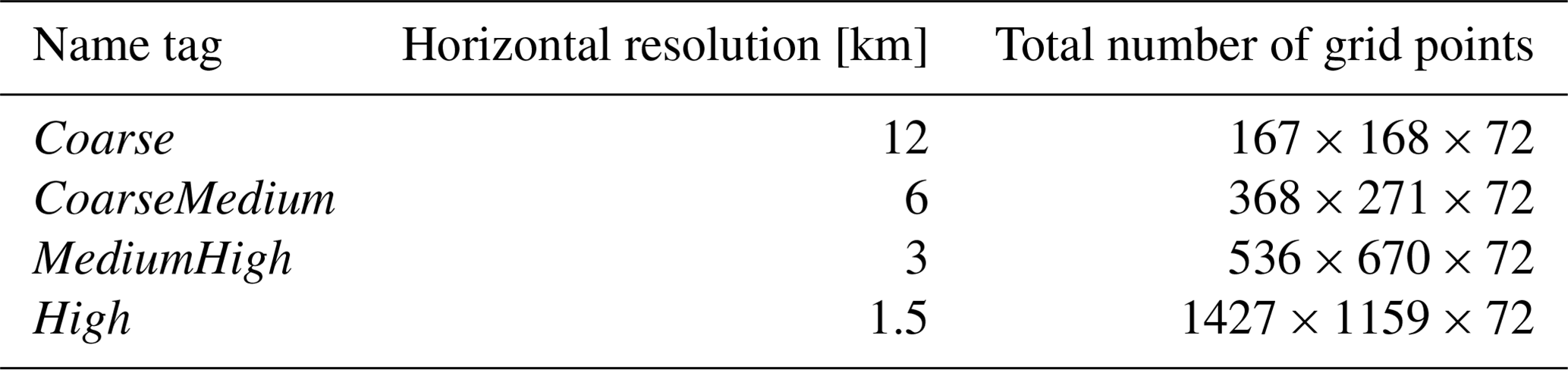
We use four configurations of a basin-scale, quasi-realistic, numerical coupled ocean circulation biogeochemical model. The configurations differ from one another in their horizontal resolutions of 12, 6, 3 and 1.5 km in a confined region of interest off Mauritania, respectively (Fig. 1, Table 1). All configurations share the same 12 km – resolution bathymetry. The ultra-high-resolution (1.5 km) configuration has been previously validated favorably in terms of ocean physics with special focus on submesoscale features by Dilmahamod et al. (2021). In the present study we explore differences that emerge as we coarsen the horizontal spatial resolution incrementally such that submesoscale features are no longer resolved. The coarsest model version is additionally integrated with altered background diffusivities and three different advection schemes. The major focus of our analysis is on diapycnal or diabatic oceanic transports, which we trace by introducing the noble gas argon as an additional prognostic tracer.

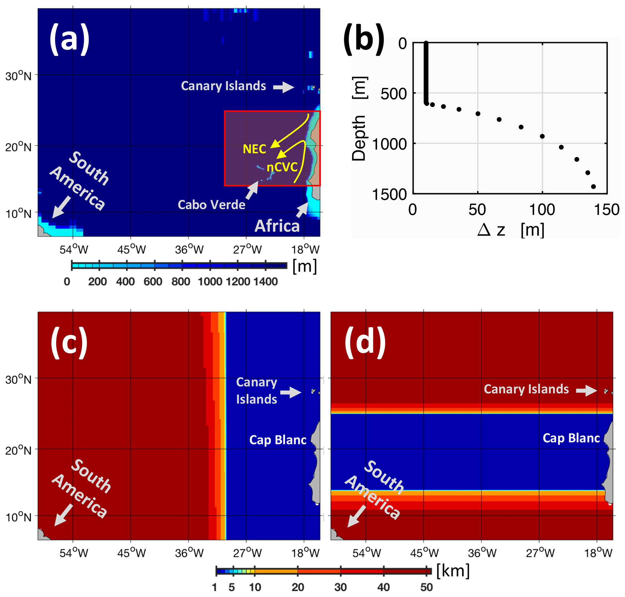
Figure 1 MOMA model domain and spatial (finite-difference) discretization. Panel (a) shows the model domain and bathymetry. The red rectangle denotes the high-resolution domain of all configurations listed in Table 1. The yellow arrows in panel (a) depict the North Equatorial Current and the northern Cape Verde Current. Their convergence defines the Cape Verde Frontal Zone. Panel (b) shows the vertical discretization of all configurations (as listed in Table 1). Panels (c) and (d) exemplarily show the zonal and meridional resolutions of the High configuration, respectively.

Table 1 List of coupled ocean circulation biogeochemical model configurations. Horizontal resolution refers to both zonal and meridional resolution within respective high-resolution domains (bounded by 14 to 25° N and 30 to 15.5° W).

2.1 Coupled ocean circulation biogeochemical model

All experiments are based on the Modular Ocean Model (MOM) framework, version MOM4p1 (Griffies, 2009), released by NOAA's Geophysical Fluid Dynamics Laboratory via https://github.com/mom-ocean/MOM4p1 (last access: 15 July 2021). The biogeochemical module is BLING – short for Biology Light Iron Nutrients and Gases developed by Galbraith et al. (2010). The model configurations are identical to the Southern Ocean setup MOMSO (≈11 km resolution Dietze et al., 2020) except for changes related to the grid, bathymetry and forcing. The high-resolution settings build on experience with the 2 km resolution configuration MOMBA (Dietze et al., 2014) and the 100 m resolution configuration MOMBE (Dietze and Löptien, 2021).

Even our highest-resolved configuration (High) applies sub-grid-scale parameterizations because it cannot resolve the full spectrum of processes (which expands down to the centimeter scale). In order to mimic the effect of unresolved vertical turbulent fluxes we apply the K-profile parameterization approach of Large et al. (1994) with a critical bulk Richardson number of 0.3 and a constant vertical background diffusivity and viscosity of ${\mathrm{10}}^{-\mathrm{5}}{\mathrm{m}}^{\mathrm{2}}{\mathrm{s}}^{-\mathrm{1}}$ in all of our coupled ocean circulation biogeochemical model simulations (unless explicitly stated otherwise, such as in Table 2). These background values also apply below the surface mixed layer throughout the water column. The choice of background diffusivity is consistent with space- and time-averaged estimates of open-ocean conditions derived by Ledwell et al. (1993) (to which substantial uncertainties in our region of interest apply, Schafstall et al., 2010). Both parameterizations of the non-local and the double diffusive (vertical) scalar tracer fluxes are applied. Horizontally, we apply a state-dependent horizontal Smagorinsky viscosity scheme (Griffies and Hallberg, 2000; Smagorinsky, 1993a, b) to keep friction at the minimal level necessitated by numerical stability. The scale of the Smagorinsky isotropic viscosity is set to a very low 0.01, which effects very low friction and thereby allows for a most vivid circulation. We do not apply any explicit horizontal diffusivity. The (default) advection scheme in the four model versions is the Sweby advection scheme of Hundsdorfer and Trompert (1994) with Sweby (1984) flux limiters. We dub our reference model setup MOMA (Modular Ocean Model off Mauritania). MOMA, in its highest-resolution configuration (High; see Table 1), has recently been favorably compared to observations by Dilmahamod et al. (2021) with a special focus on submesoscale circulation.

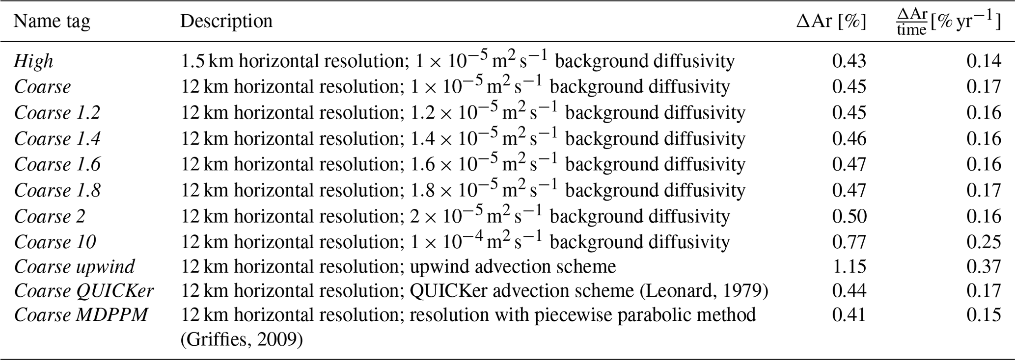
(Leonard, 1979)(Griffies, 2009)

Table 2 Simulated dissolved argon oversaturation (as a percentage) for the nominal date of 1 October 1902 averaged over depth (0 to 400 m) and the respective high-resolution model domains (bounded by 14 to 25° N and 30 to 15.5° W). Rates refer to the nominal year 1901.

2.1.1 Grid and bathymetry

We use the ETOPO5 bathymetry (National Geophysical Data Center, 1993). The bathymetry is interpolated onto an Arakawa B model grid (Arakawa and Lamb, 1977) using a bilinear scheme. The interpolated bathymetry is then smoothed with a filter similar to the Shapiro filter (Shapiro, 1970). The filter weights are 0.25, 0.5 and 0.25. The filtering procedure can only decrease the bottom depth, essentially meaning that it fills rough holes. The filter is applied three times consecutively because we found in other high-resolution model configurations that this is be a good compromise between unnecessary smoothing on the one hand and numerical instabilities introduced by overly steep topography on the other hand (Dietze et al., 2020, 2014).

Our model configurations cover almost the entire North Atlantic Ocean. The boundary is a solid rectangular wall (6.25 to 38.5° N and 15.5 to 60° W; Fig. 1a) that does not allow for any ingoing and outgoing fluxes. The design rationale is to separate boundaries and the region of interest (14 to 25° N and 30 to 15.5° W) such that spurious boundary effects fall short of entering the region of interest within our integration time of only a few years. It is for this reason that we chose a model domain that is so much larger than the region of interest.

Within the region of interest, which comprises the dynamically complex Cape Verde Frontal Zone where the North Equatorial Current meets the northern Cape Verde Current (Fig. 1a), the horizontal resolution is telescoping (Fig. 1c and d) in all of the configurations as specified in Table 1. The 12, 6, 3 and 1.5 km resolution configurations of MOMA are dubbed Coarse, CoarseMedium, MediumHigh and High, respectively (Table 1). The vertical discretization comprises a total of 72 levels in all configurations. The resolution is 10 m at the surface, coarsens to 100 m at depth and is cutoff at 1500 m. Figure 1a and b show the nominal depth and thickness of each vertical grid level, respectively. The confinement to a maximum of 1500 m water depth facilitates the use of a larger barotropic time step that reduces computational burden. Note that an additional set of simulations, as described in Sect. 2.1.3, was integrated in order to put the effect of resolution into perspective.

From Coarse to High the computational cost increases by more than 3 orders of magnitude. This increase results from the increases in zonal and meridional resolution and an overhead that is predominantly associated with the smaller time step necessitated by the increased demands in numerical stability as a consequence of the higher spatial resolution. Higher spatial resolution facilitates the simulation of faster, relatively short-lived dynamics that have to be resolved temporally in order to avoid a buildup of spurious numerical effects.

2.1.2 Initial conditions and atmospheric forcing

Initial conditions and forcing are identical to the settings in the Southern Ocean setup MOMSO, as documented in the respective model documentation (Dietze et al., 2020).

The configurations are started from rest using climatological annual mean temperatures, salinities, phosphate concentrations and oxygen concentrations from Locarnini et al. (2010), Antonov et al. (2009), Garcia et al. (2010a) and Garcia et al. (2010b), respectively. All other biogeochemical prognostic variables (such as dissolved iron concentrations and dissolved organic matter) are initialized with downscaled model output from the global fully spun up coarse-resolution configuration “FMCD” described in Dietze et al. (2017). This pragmatic decision speeds up the equilibration of biogeochemical cycles and saves computing time (but note that there are more sophisticated approaches to this problem, e.g., Khatiwala, 2024).

As for the atmospheric conditions that (in combination with the simulated surface properties of the ocean such as sea surface temperature (SST) and surface velocities) drive the fluxes of heat, moisture and momentum onto the ocean, we apply the Corrected Normal Year Forcing (COREv2) from Large and Yeager (2004, 2008) – a well-tested annual climatological cycle of all the data needed to force an ocean model (note that similar contemporary products exist, Tsujino et al., 2018; Hersbach et al., 2020). The forcing includes (artificial) synoptic variability, and air–sea fluxes evolve freely based on the bulk formula. Even so, our approach may well skew the effects of synoptic weather systems, which has been shown to be of relevance in regions of strong ocean–atmosphere coupling (e.g., O'Kane et al., 2014). Despite this caveat, Dilmahamod et al. (2021) showed that our pragmatic choice of using a climatology in MOMA produces realistic oceanic variability.

2.1.3 List of simulations

The design rationale of our simulation ensemble is to encourage the simulations to diverge from one another in response to the differences in spatial resolution, diffusivities and the choice of the advection schemes. We start in the nominal year 1900 from rest such that all configurations are shocked by the sudden onset of the atmospheric forcing, which excites waves and nonlinear circulation patterns that are free to develop independently on the respective spatial model grids. Further, we encourage diverging air–sea heat and momentum fluxes by applying nonlinear bulk formulas based on the simulated oceanic surface properties in the respective calculations.

We compare simulations that have not yet reached equilibrium (after 1 year of spin-up and a relatively short overall integration time of a maximum of 3 years), which limits potentially spurious effects of our lateral boundary conditions (see Appendix B) and saves computational resources. Note in this context that Dilmahamod et al. (2021) showed that the circulation of MOMA is already realistic after a spin-up of only one seasonal cycle. Consistent with this result, we find that the energy content of our eddy field does not fall short of observational estimates after 1 year (Fig. 5). This suggests that our simulation period of 3 years is long enough to reveal major effects of differing resolution (even though it may take much longer to equilibrate potential energy).

We integrate two sets of model simulations. The first set features four differing resolutions, as listed in Table 1. These simulations are dubbed Coarse, CoarseMedium, MediumHigh and High.

The second set of simulations is targeted at putting the differences among the first set into perspective. The focus is on effective domain-averaged diapycnal mixing between Coarse and High as traced by simulated argon saturation. The simulations explore a range of (uncertain) parameter settings for the vertical background mixing and diffusivity (Coarse 1.2, Coarse 10) and numerical advection schemes (Coarse upwind, Coarse QUICKer, Coarse MDPPM) (Sect. 2.2.1, Table 2).

2.2 Model analyses

We focus on ranking the effective diapycnal mixing in our simulations against one another. Effective diapycnal mixing is infamously difficult to quantify in models (Griffies et al., 2000; Megann, 2018; Burchard and Rennau, 2008; Getzlaff et al., 2012). Here we add to the discussion by introducing dissolved argon as an additional prognostic tracer to our simulations in order to track mixing by respective oversaturation.

2.2.1 Argon saturation – a proxy for mixing

As suggested by Dietze and Oschlies (2005b), we employ an explicit representation of argon in our suite of configurations in order to trace the effect of mixing: argon (Ar) is a noble gas and once isolated from the sea surface is a conservative tracer in the ocean (e.g., Bieri et al., 1966). Argon oversaturation, ΔAr, is defined as follows:

$$\begin{array}{}\text{(1)}& {\displaystyle }{\displaystyle }\mathrm{\Delta }\mathrm{Ar}={\displaystyle \frac{\mathrm{Ar}}{{\mathrm{Ar}}_{\text{sat}}}}\times \mathrm{100}\mathrm{\%}-\mathrm{100}\mathrm{\%},\end{array}$$

where Ar and Ar_sat denotes the actual and saturated Argon concentrations, respectively. In contrast to the concentration, the saturation is not conservative. A mixed water parcel will always carry a higher argon saturation than the arithmetic mean of the original parcels since the saturation curves are convex over the entire range of oceanic temperatures (and salinities). Hence, an increase in ΔAr % may be indicative of mixing (while negative values can be indicative of spurious dispersion).

Even though there is consensus on the link between mixing and ΔAr (Dietze and Oschlies, 2005b; Ito and Deutsch, 2006; Henning et al., 2011; Ito et al., 2007; Emerson et al., 2012; Hamme et al., 2017; Getzlaff et al., 2019), a ubiquitous relationship between standing stocks of argon saturation and diapycnal mixing that would allow for a global localized assessment of effective diffusivities in numerical models has not been established yet. Among the challenges yet to be overcome is to correct for processes other than mixing that affect ΔAr, such as subsurface warming by penetrating solar radiation (e.g., Dietze and Oschlies, 2005a) and bubble entrainment (e.g., Spitzer and Jenkins, 1989; Hamme et al., 2017).

In this study a ubiquitous relationship is not targeted. Instead, we aim to use ΔAr as a relative measure to rank our simulations with respect to mixing against one another. To this end our simulated argon concentrations are more of a simple analytical tool designed to compare simulations among one another rather than a metric capable of constraining the absolute effective mixing in models with observations (such as developed by Holmes et al., 2021). This facilitates the implementation because we can initialize all simulations with ΔAr=0 % and are not bound to integrate until the saturations have equilibrated because we only study the differences between our simulations rather than linking simulated concentrations to observations.

3 Results

A comprehensive and favorable comparison between the High simulation and observations is provided by Dilmahamod et al. (2021). Here we focus on illustrating that our High simulation is capable of resolving submesoscale features. Further, we will employ ΔAr to compare simulations with respect to the effect of diapycnal mixing.

3.1 Resolving mesoscale and submesoscale dynamics

Figure 2 shows a sea surface temperature snapshot of the entire model domain after 2 years, 3 months and 11 d of spin-up. The simulated sea surface temperatures look very similar both outside and inside the high-resolution domain. Differences between the resolutions only become apparent at extreme zoom levels such as the one shown in Fig. 3 for an upwelling filament off Cap Blanc. On these scales it is evident that a higher spatial model resolution clearly improves the representation of small circulation features, such as the relatively warm SST feature near 21° N, 18° W that is completely absent in Coarse. Figure 4 confirms the visual impression of increasing levels of detail with increasing resolution by showing respective vertical relative vorticities, which are calculated as follows:

$$\begin{array}{}\text{(2)}& {\displaystyle }{\displaystyle }{\mathit{\zeta }}^z=\partial {}_{x}v-\partial {}_{y}u,\end{array}$$

which is normalized by the Coriolis frequency f. Given that submesoscale structures are associated with values of magnitude O(1) (e.g., Shcherbina et al., 2013), Fig. 4 shows that the Coarse and CoarseMedium configurations are devoid of submesoscale dynamics, while MediumHigh features sporadic occurrences and High ubiquitous coverage. This warrants a comparison between submesoscale and coarser resolutions using our Coarse and High configurations.

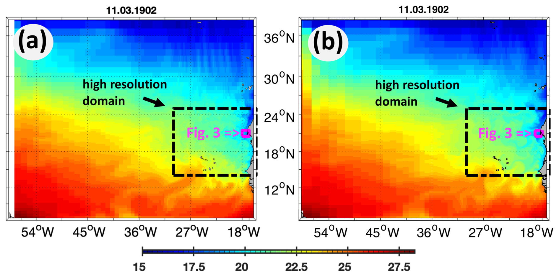
Figure 2 Example snapshots of simulated sea surface temperatures (in °C). Panels (a) and (b) feature the entire model domain of the high-resolution configuration High and the coarse-resolution configuration Coarse, respectively. The dashed black line denotes the region where both zonal and meridional resolution telescopes (Fig. 1) as specified in Table 1. The tiny magenta squares off Cap Blanc at the coast of Mauritania depict the boundaries of the zoom shown in Fig. 3.

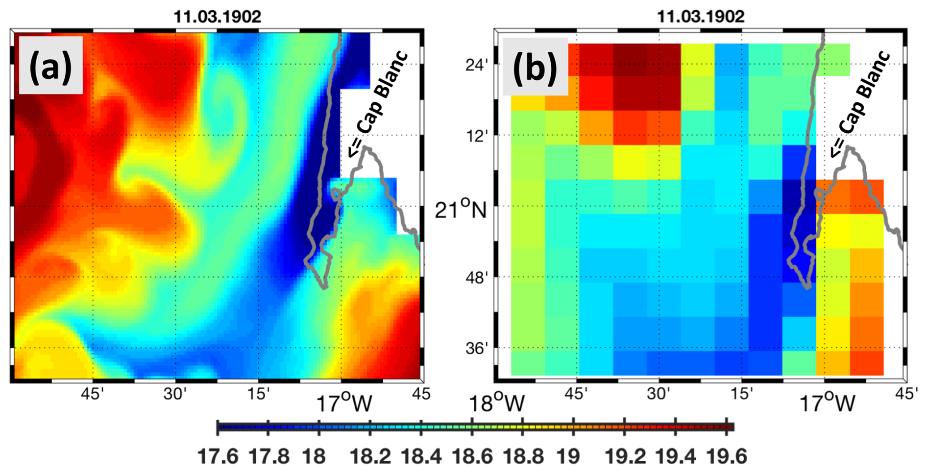
Figure 3 Example snapshots of simulated sea surface temperatures capturing an upwelling filament off Cap Blanc. Panels (a) and (b) show the high-resolution configuration High and the coarse-resolution configuration Coarse, respectively. Note that the entire model domain is larger than shown here (Fig. 2).

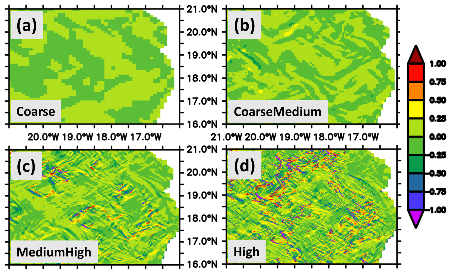
Figure 4 Example snapshot of simulated vorticity during the upwelling period (nominal date of 15 January 1902). The vorticity is calculated from surface currents averaged over the upper 50 m and normalized by the Coriolis frequency. Panels (a)–(d) showcase the effect of horizontal resolution in our configurations. A relative vorticity of magnitude O(1) indicates submesoscale flows. The region shown corresponds to ≈15 % of the area of the high-resolution model domain.

Figure 5 shows eddy kinetic energy (EKE) averaged meridionally over the respective high-resolution model domain as observed from space and simulated with the High and Coarse simulations. As to be expected, the eddy kinetic energy increases with higher spatial resolution because the submesoscale circulation starts to contribute to the integrated energy spectrum. Hence, theHigh simulation features higher EKE levels than Coarse (also because the energy cascade from large to smaller spatial scales is apparently not accelerated by the increase in resolution). EKE in both High and Coarse does not fall short of observational estimates (during neither the upwelling nor the relaxation season). This implies that the simulations capture enough dynamics for a meaningful comparison of the differing configurations (as a comparison of High and Coarse with overly sluggish circulations would be inconclusive). We also note that Dilmahamod et al. (2021) find no evidence for excessive overestimation of our simulated eddy dynamics in the High simulation, while at the same time there is evidence that eddy kinetic energy estimates from space are biased low (e.g., Fratantoni, 2001; see also Luecke et al., 2020, for agreements between models and observations across frequency bands).

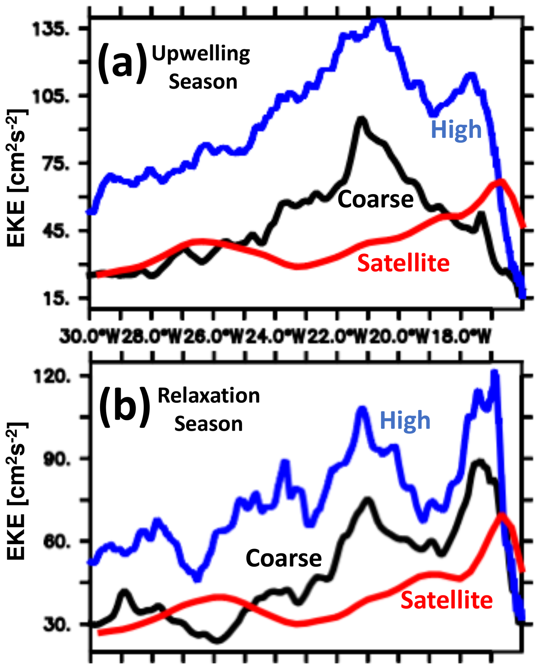
Figure 5 Eddy kinetic energy that has been domain averaged over the high-resolution model domain (17–24° N, 30–15° W). Panels (a) and (b) refer to the upwelling season (December–April) and the relaxation season (May–July), respectively. The red line refers to observations from space (Aviso 1993–2010). The black and blue lines denote model output averaged over the nominal years 1901–1902 simulated with the High and Coarse configuration, respectively.

Small-scale mesoscale and submesoscale features have been associated with locally intensified vertical fluxes (e.g., Lévy et al., 2001; Mahadevan and Archer, 2000; Mahadevan and Tandon, 2006; Martin and Pondaven, 2003). Consequently, it has been argued that vertical exchange should increase along with spatial resolution since ever more small-scale features are resolved with increasing resolution. One of the processes potentially leveraging this effect is surface current wind interaction (Martin and Richards, 2001). Ekman pumping is calculated from the curl of the wind stress. The resolution of ever smaller spatial scales in ocean currents yields higher spatial derivatives of wind stress, calculated from the squared difference in wind speed and oceanic surface current velocity. Hence, simulated Ekman pumping, associated with the wind stress curl, increases with model resolution. Table 3 confirms that higher resolution yields higher Ekman velocities in our configurations. This applies for both the mean of the magnitude and the standard deviation, which approximately double from Coarse to High. Figure 6 showcases the signature of ocean circulation in the Ekman pumping in more detail. In Coarse the prevalent structure is boxlike with a spatial scale of O(100 km) affected by the scale of the (spatially discretized) atmospheric forcing. Increasing the resolution to that of CoarseMedium, MediumHigh and High results in ever more structure, which is apparently related to an eddying circulation with local values increasing up to several meters per day. Hence, we expect, consistent with the pioneering work of, e.g., Lévy et al. (2001); Mahadevan and Archer (2000); Mahadevan and Tandon (2006); Martin and Pondaven (2003), an increase in vertical fluxes of heat, salt and biogeochemical entities with increasing resolution in our configurations. We are particularly curious whether the increase in Ekman dynamics with increasing resolution leads to enhanced diapycnal mixing or if its effect is primarily advective.

Table 3 Ekman pumping as simulated within the high-resolution model domains on nominal 15 January 1901 in units of m d⁻¹.

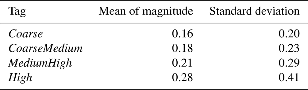
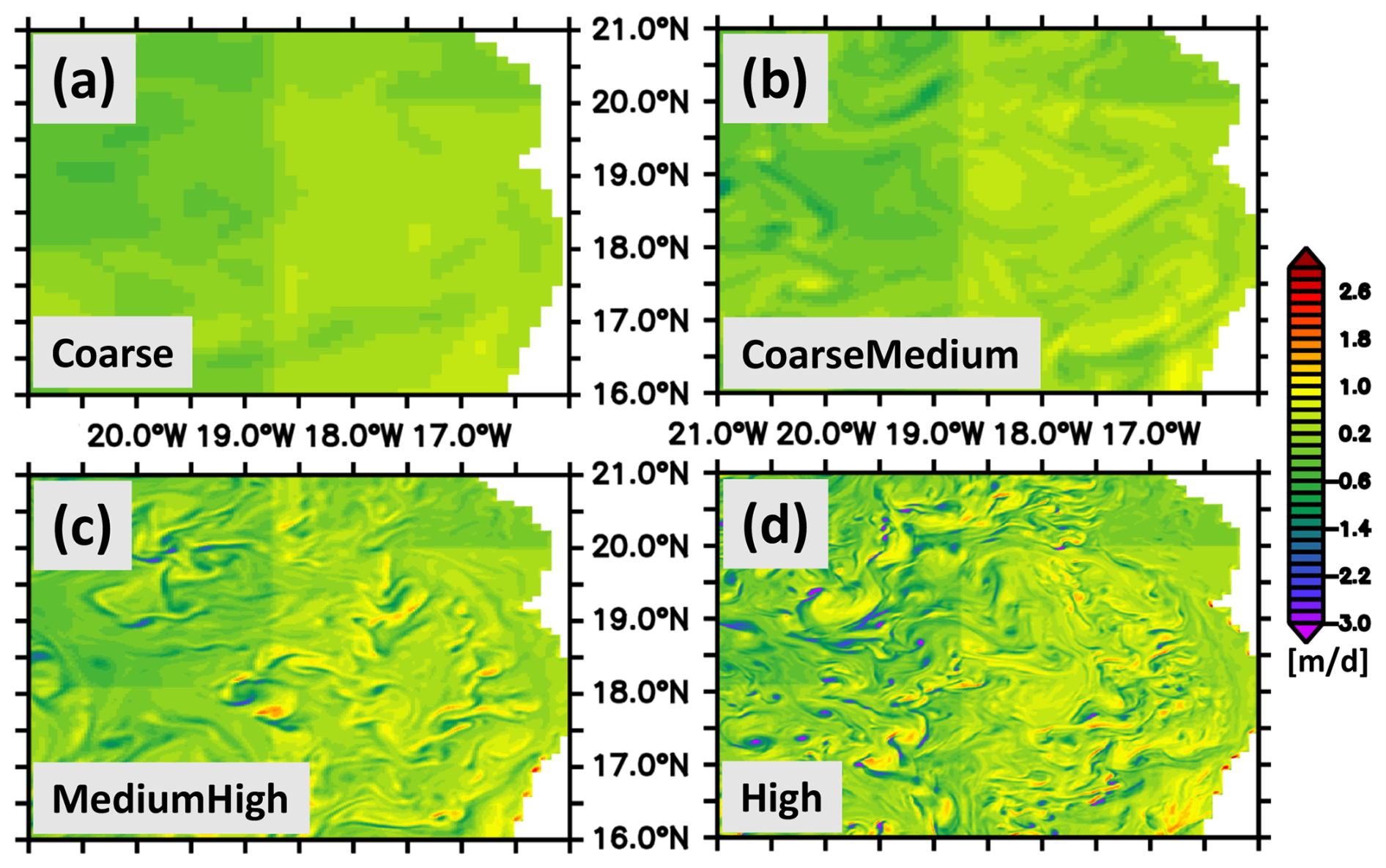
Figure 6 Example snapshot of simulated Ekman pumping (nominal date of 15 January 1901). The Ekman pumping includes surface current wind effects. Panels (a–d) refer to the Coarse, CoarseMedium, MediumHigh and High configurations, respectively. The region shown corresponds to ≈15 % of the area of the high-resolution model domain.

3.2 Ocean mixing

Based on previous work (e.g., Lévy et al., 2001; Mahadevan and Archer, 2000; Mahadevan and Tandon, 2006; Martin and Pondaven, 2003) we expect an increase in vertical mixing in response to increasing resolution of intense and localized upwelling and downwelling events. Alternatively, we may find that the effect of such events cancels out on larger scales in our model (Reissmann et al., 2009; Eden and Dietze, 2009; Dietze and Löptien, 2016).

In this section, we use argon oversaturation as a proxy recording the mixing history of water parcels since these were last in contact with equilibrating air–sea fluxes at the sea surface. We start with an illustration of effects, continue with comparing the different spacial resolutions and end with putting the latter into perspective by comparing them to other simulations.

The interpretation of argon saturation is not straightforward because it is antagonistically affected by mixing. Diapycnal mixing produces oversaturation, as explained in Sect. 2.2.1. At the same time, however, mixing transports oversaturated water to the surface where it loses its oversaturation to the atmosphere. Figure 7a shows a Hovmöller diagram of the argon saturation averaged over the high-resolution domain that illustrates the antagonistic processes at work. Above the surface mixed layer the water is always saturated because it is subject to equilibrating air–sea fluxes. Below the surface mixed layer the water is shielded from the direct effect of air–sea fluxes, and three effects prevail in our simulations. (i) Solar radiation penetrating below the surface mixed layer increases the temperature in summer. This reduces the solubility and increases the saturation (e.g., Dietze and Oschlies, 2005a). (ii) Mixing of water parcels (affected by the sum of explicitly prescribed diffusivity and implicit spurious mixing from numerical schemes) with differing temperatures and salinities results in oversaturation because solubility is a nonlinear function of temperature and salinity (e.g., Dietze and Oschlies, 2005b; Ito and Deutsch, 2006; Emerson et al., 2012). (iii) Mixing occurs between equilibrated surface water across the surface mixed layer and abyssal water still carrying the initial 0 % oversaturation. In combination, these effects drive a seasonal saturation maximum situated directly below the surface mixed layer and a linearly downward-protruding saturation signal over time.

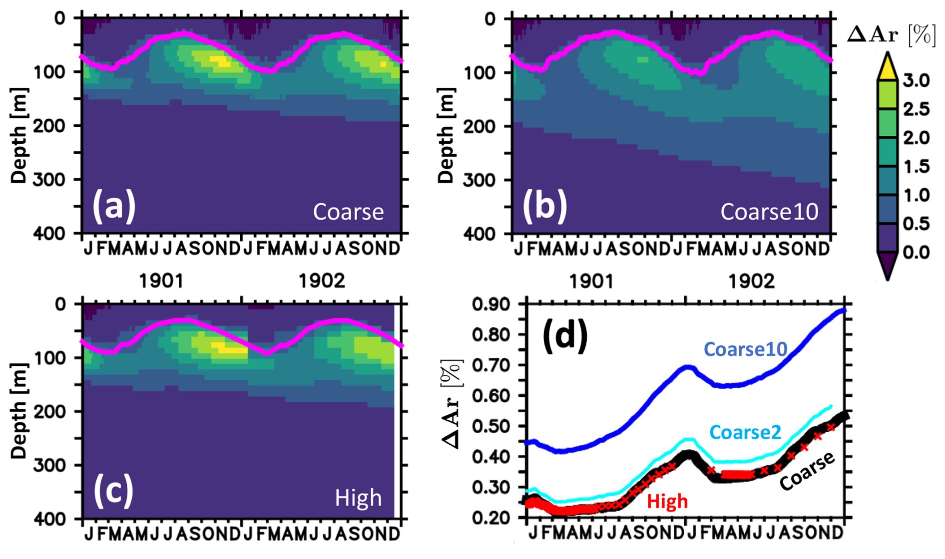
Figure 7 Simulated argon oversaturation (as a percentage) averaged over the high-resolution model domain (17–24° N, 30–15° W). Panels (a)–(c) refer to model configurations Coarse, Coarse10 (featuring a 10-fold increase in background diffusivity relative to Coarse) and High, respectively. The magenta line denotes the surface mixed layer defined with a Δ=0.5 K temperature criterion. Panel (d) shows corresponding oversaturation averaged over 100 to 400 m depth for the High, Coarse, Coarse2 and Coarse10 configurations. Coarse2 refers to a simulation with a 2-fold increase (from 1 to $\mathrm{2}\times {\mathrm{10}}^{-\mathrm{5}}{\mathrm{m}}^{\mathrm{2}}{\mathrm{s}}^{-\mathrm{1}}$) in background diffusivity.

A comparison between Fig. 7a and b, showing results from Coarse and Coarse10 (Table 2), respectively, reveals how an (exaggerated) 10-fold increase in explicitly prescribed background diffusivity manifests itself: the higher diffusivity smoothes the maximum below the surface mixed layer by distributing the saturation signal vertically. Part of the signal enters the surface mixed layer and is eradicated by equilibrating air–sea fluxes while part of it is protruding downwards. When computing water column averages below the surface, we see in Fig. 7d that Coarse10 accumulates deep oversaturation at a faster pace than Coarse even though its losses to the ventilated surface mixed layer are greater due to enhanced vertical exchange by mixing. Note that this also applies when averaging over the entire water column (not shown). A comparison between High, Coarse and Coarse10 in Fig. 7 suggests that the effective diapycnal mixing in High is not larger than in Coarse because High features a similar or smaller increase relative to Coarse. Near the end of the simulation, the averaged ΔAr in the 100 to 400 m depth range amounts to 0.43 % in High relative to 0.45 % in Coarse. In addition, the visual impression of the simulated argon saturation for Coarse and High in Fig. 7a and c is rather similar, while Fig. 7b is distinctly different.

Table 2 and Fig. 9 put the small differences in simulated averaged oversaturation values between High and Coarse into perspective. From a suite of simulations with background diffusivities of 1, 1.2, 1.4, 1.6, 1.8, 2 and $\mathrm{10}\times {\mathrm{10}}^{-\mathrm{5}}{\mathrm{m}}^{\mathrm{2}}{\mathrm{s}}^{-\mathrm{1}}$, we conclude that our method can reliably detect differences in background diffusivity down to $\mathrm{0.4}\times {\mathrm{10}}^{-\mathrm{5}}{\mathrm{m}}^{\mathrm{2}}{\mathrm{s}}^{-\mathrm{1}}$ but fails at distinguishing very low diffusivities. This is probably because the implicit numerical diffusion is then masking the effects of our choices of explicit diffusivity.

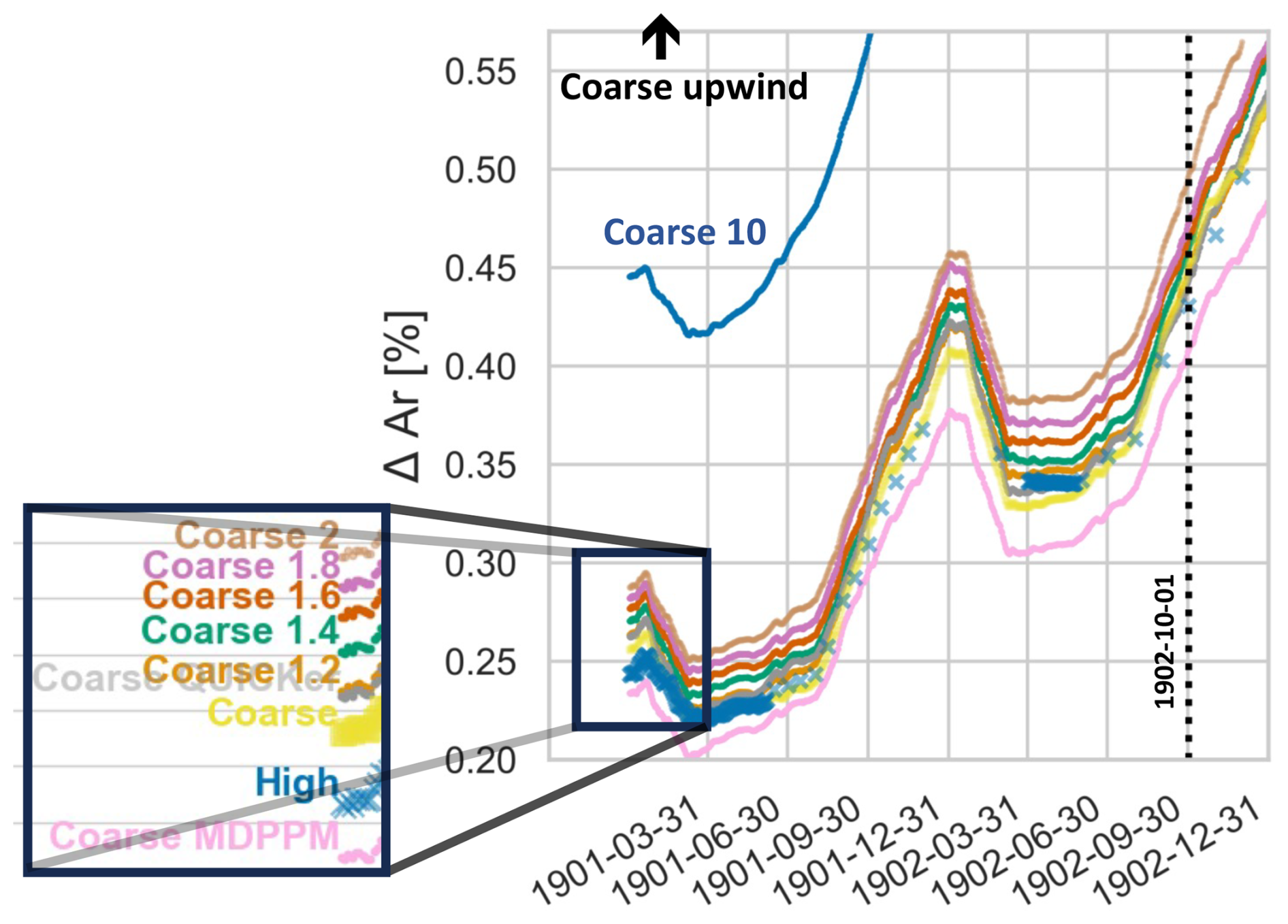
Figure 8 Temporal evolution of simulated argon oversaturation (as a percentage) averaged over the high-resolution model domain (17–24° N, 30–15° W) and 100 to 400 m depth starting after the first year of spin-up. Data gaps such as those in the High configuration are attributable to I/O failures. The dashed black line marks the nominal date of October 1902, which is the basis for the data in Table 2. The Coarse upwind configuration is off the scale. Model tags are explained in Table 2.

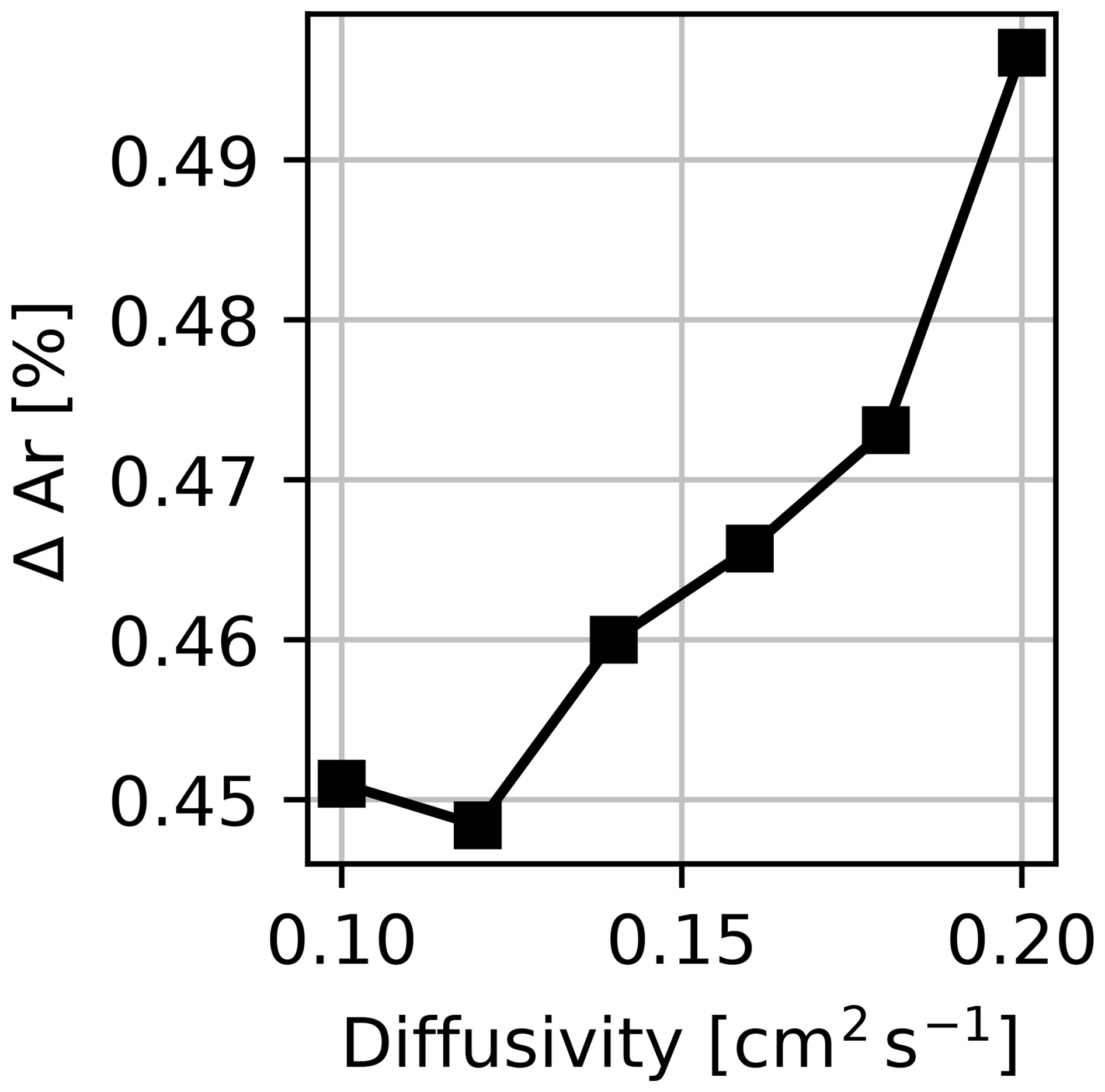
Figure 9 Simulated argon oversaturation as a function of explicit background diffusivity. Each value corresponds to a Coarse simulation with respective diffusivity for temperature, salinity and argon. The argon oversaturation is calculated as being averaged horizontally over the high-resolution model domain (17–24° N, 30–15° W) and vertically over 100 to 400 m depth. For reference, the High simulation features 0.43 % (Table 2).

Overall, we conclude that the difference between the High and Coarse simulations in terms of diffusivity as detected by argon saturation is rather minor and comparable to other infamous and contemporary uncertainties such as switching from one state-of-the-art advection scheme to another (Table 2; default scheme in Coarse vs. Coarse QUICKer and Coarse MDPPM). Note that in this context the effect of using the outdated upwind scheme introduces much larger effects on the diapycnal mixing and that this effect is even stronger than a 10-fold increase (Coarse 10) in background diffusivity.

3.3 Discussion

Our study exploits the nonlinear convex relationship between argon saturation and temperature (and salinity) in order to rank effective diapycnal mixing in a suite of model simulations. Our range of calibration simulations where the background diffusivity was varied between $\mathrm{1}\times {\mathrm{10}}^{-\mathrm{5}}{\mathrm{m}}^{\mathrm{2}}{\mathrm{s}}^{-\mathrm{1}}$ and $\mathrm{1}\times {\mathrm{10}}^{-\mathrm{4}}{\mathrm{m}}^{\mathrm{2}}{\mathrm{s}}^{-\mathrm{1}}$ show that simulations with differences in background diffusivities of more than $\mathrm{4}\times {\mathrm{10}}^{-\mathrm{6}}{\mathrm{m}}^{\mathrm{2}}{\mathrm{s}}^{-\mathrm{1}}$ are consistently different in that higher diffusivities are associated with higher saturations throughout the second and third years of the simulation (Figs. 8 and 7 and Table 2).

Clearly, the saturation signals due to mixing are low in amplitude. This obstructs a comparison of our model output with real-world observations where additional antagonistic processes such as bubble entrainment and effects of finite gas exchange that can fail to keep up with the cooling effect on saturation in convective regimes (e.g., Seltzer et al., 2023) are at play. The representation of these effects is at present still dependent on model formulations, and solving this issue is a work in progress (e.g., Pöppelmeier et al., 2023) driven by an increasing observational base and growing general interest (e.g., Jenkins et al., 2023; Hamme et al., 2017). Nonetheless, our results show that our method consistently ranks simulations with varying background diffusivity and advection schemes, suggesting the robustness of argon saturation as a comparative metric. The next question is how it compares to other contemporary approaches when diagnosing diffusivities in model simulations.

The main advantage of our method is its simplicity. Typically all models provide an interface to add a passive tracer so that our implementation of argon to trace mixing reduces to merely calculating initial conditions (i.e., 100 % saturation based on initial temperatures and salinities) and setting of a surface boundary condition where argon is reset to 100 % saturation every time step. This sets it apart from more sophisticated approaches based on variance decay (e.g., Burchard and Rennau, 2008; Schlichting et al., 2023) or available potential energy (e.g., Ilicak, 2016).

Our approach based on argon saturation is apparently similar to the approach of Holmes et al. (2021) that is based on diffusively effected heat fluxes. First, we find that their diffusively effected heat fluxes yield qualitatively similar patterns to our estimates of “diffusively effected” argon fluxes (Fig. A1 of Holmes et al., 2021, vs. Fig. 3 in Dietze and Oschlies, 2005b). Second, we report a detection accuracy of down to $\mathrm{4}\times {\mathrm{10}}^{-\mathrm{6}}{\mathrm{m}}^{\mathrm{2}}{\mathrm{s}}^{-\mathrm{1}}$, which is similar to what we derive from Fig. 17 in Holmes et al. (2021) where their simulations 025-NG0, 025-KBV and 025KB5 showcase that their approach can detect changes in diffusivities down to $\mathrm{5}\times {\mathrm{10}}^{-\mathrm{6}}{\mathrm{m}}^{\mathrm{2}}{\mathrm{s}}^{-\mathrm{1}}$.

4 Conclusions

We implemented an explicit prognostic representation of dissolved argon into an ocean circulation biogeochemical model of the North Atlantic. A suite of calibration simulations with systematically altered background diffusivities established a link between argon saturation and effective vertical diffusivity. This link was employed to rank effective diffusivity in a suite of model configurations with differing spatial resolutions off Mauritania against one another. Further, we tested different numerical advection schemes in order to set the resolution effects into perspective.

Our results suggest rather modest effects that are comparable to contemporary numerical errors when switching from a 12 km mesoscale to a 1.5 km submesoscale resolution. More specifically, we find the effect on argon based on this change in resolution is comparable to a change to another contemporary advection scheme or to a change in the background diffusivity of less than 60 % (note that all of these minor effects appear below the detection limit of our method, whereas larger changes in diffusivity could be clearly identified).

Our results are in line with recent findings of Brett et al. (2023) and Karleskind et al. (2011), who reported on surprisingly large similarities between submesoscale-resolving simulations and the same simulations with an artificially damped circulation.

However, caveats apply to these conclusions. Among these caveats are that (1) we applied a hydrostatic approximation which is also used in contemporary Intergovernmental Panel on Climate Change (IPCC) models (in contrast to, e.g., Mahadevan and Archer, 2000); (2) the effects of a combined increase in horizontal and vertical resolution have not been tested (see Stewart et al., 2017, for background information); (3) our results might only apply for the region off Mauritania; and (4) the potentially accumulating long-term effects of differing resolutions have not been studied.

Appendix A: Generic model output

The main body of the paper is focused on effective vertical mixing as traced by argon saturation rather than showcasing results from the suite of simulations. Here, we present more generic model output, such as simulated air–sea fluxes, export production, and simulated dissolved oxygen. We focus on averages covering the respective highly resolved subdomains rather than going for side-by-side comparisons between snapshots. The reason is that eddying model simulations are known to show a highly nonlinear behavior that can manifest itself in notable differences even in repetitions of the exact same experiment using identical executables and hardware (e.g., Dietze et al., 2014, “computational uncertainty” in their Fig. 21). Further, detailed differences between individual circulation features may be considered irrelevant in the context of IPCC-type modeling if they average out on the larger spatial scales that are applicable to coupled components such as the atmosphere.

Among the oceanic peculiarities in the region of interest is an exceptionally complex seasonally varying coastal circulation including deep-reaching undercurrents. Figure A1 shows an example as resolved in exemplary snapshots by the High and Coarse configurations. During the upwelling season, High features a double-cored poleward undercurrent consistent with observations at 18° N (Dilmahamod et al., 2021, their Fig. 2). Coarse is similar but features overall weaker currents. This makes it less realistic in terms of its representation of the undercurrent and more realistic in terms of its representation of the near-surface equatorward current on the shelf. During the relaxation season, an intensification of wind stress curl induces an intensification of poleward flow. This, along with ebbed-away equatorward surface current, is reproduced by both High and Coarse. In summary, Coarse is strikingly similar to High in terms of seasonality and spatial structure of near-coastal currents, except for resolving fewer small-scale details.

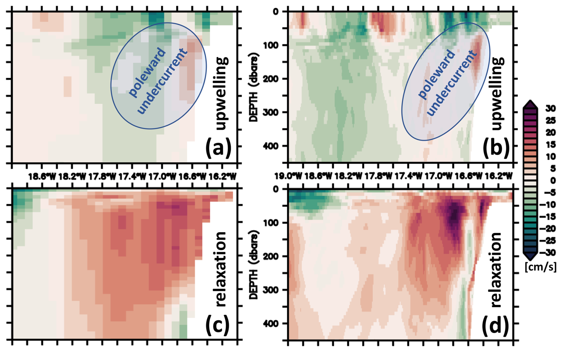
Figure A1 Simulated alongshore currents for the Coarse (a, c) and High (b, d) configurations along a zonal section at 18° N. Panels (a) and (b) refer to exemplary snapshots during the upwelling season (nominal date of 1 February 1902), while (c) and (d) refer to the relaxation season (nominal date of 1 June 1901).

These similarities of complex seasonal coastal dynamics may, despite the fact that they appear very small, still allow for substantially differing distributions of heat and salt due to the nonlinear nature of the system. This may be of particular relevance for those surface properties that couple the ocean with the atmosphere (such as SST). Table A1 illustrates, however, that domain-averaged sea surface temperatures, sea surface salinities and near-surface nutrients also differ very little across the model configurations. Further, these differences are not all monotonically aligned with the spatial model resolution, which suggests there must be other reasons for the (very small) differences between the configurations.

Table A1 Sea surface temperature (SST), sea surface salinity (SSS) and phosphate concentration simulated with respective model configurations (resolutions). All values are averaged over the respective high-resolution model domains (bounded by 14 to 25° N and 30 to 15.5° W) at the end of the simulation on the nominal date of 31 December 1902. Phosphate concentrations refer to vertical averages over the euphotic zone (0–120 m depth).

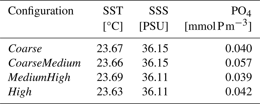
Figure A2 provides evidence that the small SST differences do not amplify to considerable air–sea heat flux differences: the exemplary snapshots after almost 3 years of spin-up are – irrespective of resolution – strikingly similar, with the only difference being the amount of small-scale structure resolved (which may or may not be associated with Ekman pumping driven by the surface current wind effects described above). This is consistent with the rather low sensitivity of effective diffusivity as traced by argon saturation in Sect. 3.

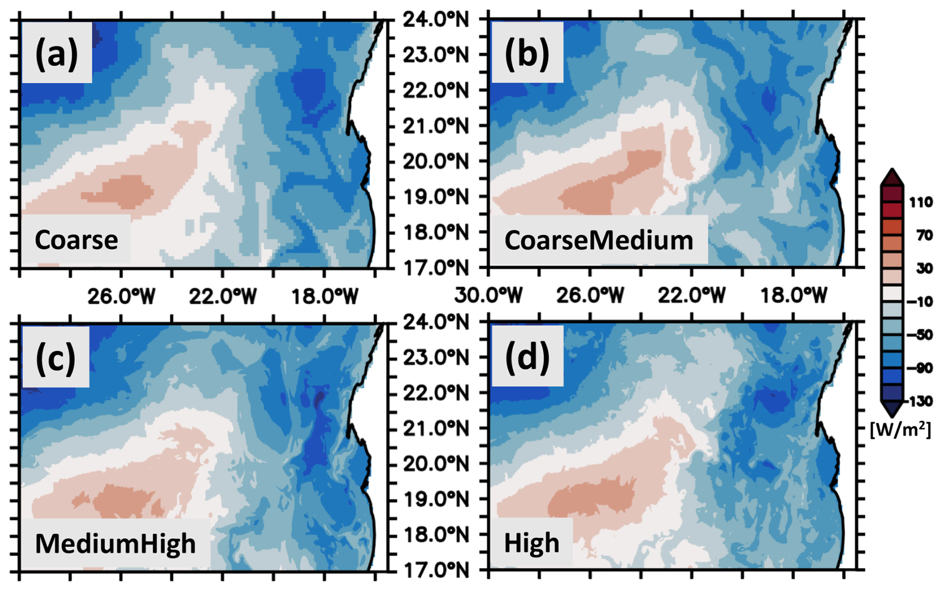
Figure A2 Snapshot of simulated daily mean air–sea heat flux (nominal date of 17 December 1902). Panels (a)–(d) refer to the Coarse, CoarseMedium, MediumHigh and High configurations, respectively. Positive numbers denote oceanic heat gain.

In the following our focus is on domain-averaged persistent effects that may be missed by configurations with coarse resolutions rather than on local small-scale transient phenomena. Figure A3a shows the ensemble mean domain-averaged seasonal heat flux. In line with results from Faye et al. (2015) and Foltz et al. (2013), we find a substantial seasonality ranging from a 200 W m⁻² oceanic heat loss in winter up to a 100 W m⁻² heat gain in summer. Figure A3b shows that the difference among the configurations is on the order of a few W m⁻², corresponding to deviations of several percent only. These differences are well within the uncertainty range even for observational estimates (e.g., Gulev et al., 2007). In addition, we again report that there is no apparent consistent relationship between the deviation from the ensemble mean and the spatial model resolution.

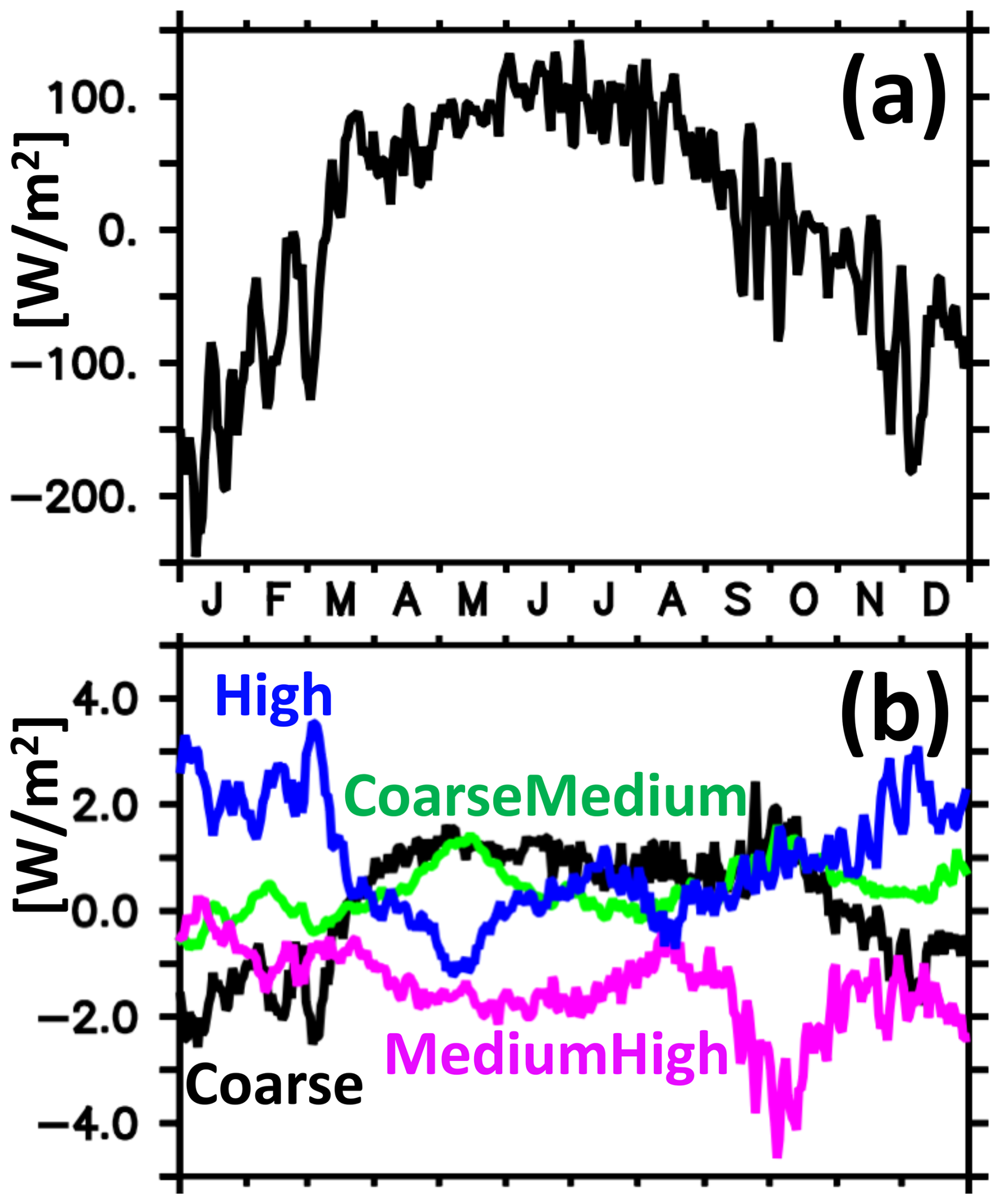
Figure A3 Simulated mean air–sea heat flux averaged over the high-resolution model domain (17–24° N and 30–15° W) (nominal year 1902). Panel (a) shows the ensemble mean of the Coarse, CoarseMedium, MediumHigh and High configurations. Positive numbers denote oceanic heat gain. Panel (b) shows the respective differences from the ensemble mean.

Similar conclusions apply to simulated biogeochemical entities. The vertical gradients of temperature and nutrients typically oppose one another, with warm sunlit surface waters being depleted in nutrients (essential for phytoplankton growth) and cold abyssal waters being replete with nutrients. Enhanced vertical transports are expected to increase oceanic heat gain by exposing additional cold water to the relatively warm atmosphere (in our region of interest). Similarly, enhanced vertical transport results in an increase in nutrient availability to phytoplankton at the sunlit surface, which should manifest itself in, e.g., increased biotic export production. Figure A4a shows the ensemble mean domain-averaged export production over the course of the year with peaking values between 40 and $\mathrm{50}\mathrm{mmol}\mathrm{P}{\mathrm{m}}^{-\mathrm{2}}{\mathrm{yr}}^{-\mathrm{1}}$ during the spring bloom and wintertime values of only several $\mathrm{mmol}\mathrm{P}{\mathrm{m}}^{-\mathrm{2}}{\mathrm{yr}}^{-\mathrm{1}}$. Throughout this strong seasonal cycle, the individual configurations deviate only a few $\mathrm{mmol}\mathrm{P}{\mathrm{m}}^{-\mathrm{2}}{\mathrm{yr}}^{-\mathrm{1}}$ from the ensemble mean, and there is again no consistent relationship between deviation and resolution (Fig. A4b).

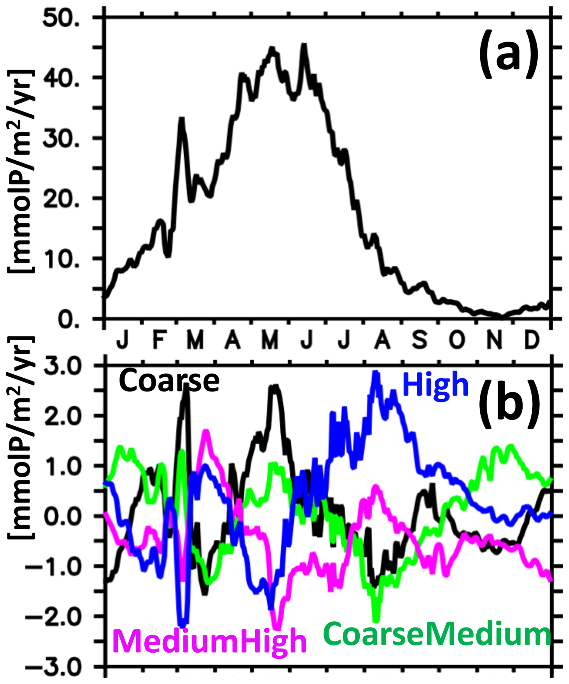
Figure A4 Simulated export production calculated as net biotic phosphate sources and sinks integrated over the upper 150 m water column and averaged over the high-resolution model domain (17–24° N and 30–15° W) (nominal year 1902). Panel (a) shows the ensemble mean of the Coarse, CoarseMedium, MediumHigh and High configurations. Panel (b) shows the respective differences from the ensemble mean.

A1 Dead-zone eddies – a case study

Among the regional peculiarities off Mauritania are the anticyclonic mode water eddies (ACMEs) that travel from the shelf break hundreds of kilometers offshore carrying a body of low-oxygen water (Karstensen et al., 2015). Scientific interest in these “dead-zone eddies” includes the study of the sensitivity of organisms to oxygen deficit (Hauss et al., 2016). Here, we present them as episodic events benchmarking the effect of resolution. Our interest is rooted in the fact that ACMEs are highly nonlinear events shaped by an interplay of complex ocean circulation with biogeochemical cycles. Our rationale is that this nonlinearity could amplify the rather insignificant differences in metrics discussed so far. To this end, the following dead-zone eddy case study is designed to find differences between the resolutions that may be of relevance to other components of the Earth system, such as higher trophic levels and fisheries.

Figure A5 shows a respective comparison between Coarse and High. Figure A5a and b start with showcasing an anticyclonic mode water eddy (ACME) being shed off the Mauritanian shelf. An analysis of underlying dynamics is provided by Dilmahamod et al. (2021), and a more comprehensive visualization of processes is animated in Dietze and Löptien (2023). Both High and Coarse feature a pronounced seasonal cycle of dissolved oxygen concentration on the shelf, which is consistent with results from Mittelstaedt (1991). During the upwelling season the shelf is sheltered from relatively cool and oxygen-rich upwelling waters offshore. The biotic production on the shelf is exceptionally high (e.g., Wolff et al., 1993), and this fuels declining levels of oxygen at depth. In line with Mittelstaedt (1991), we find that the isolation of shelf water is permeated by occasional export events. Figure A5a and b show such export events in the High and Coarse configurations, respectively. ACMEs seeded with low-oxygen shelf water are formed and travel offshore for months (Fig. A5c and d) retaining their low-oxygen signature.

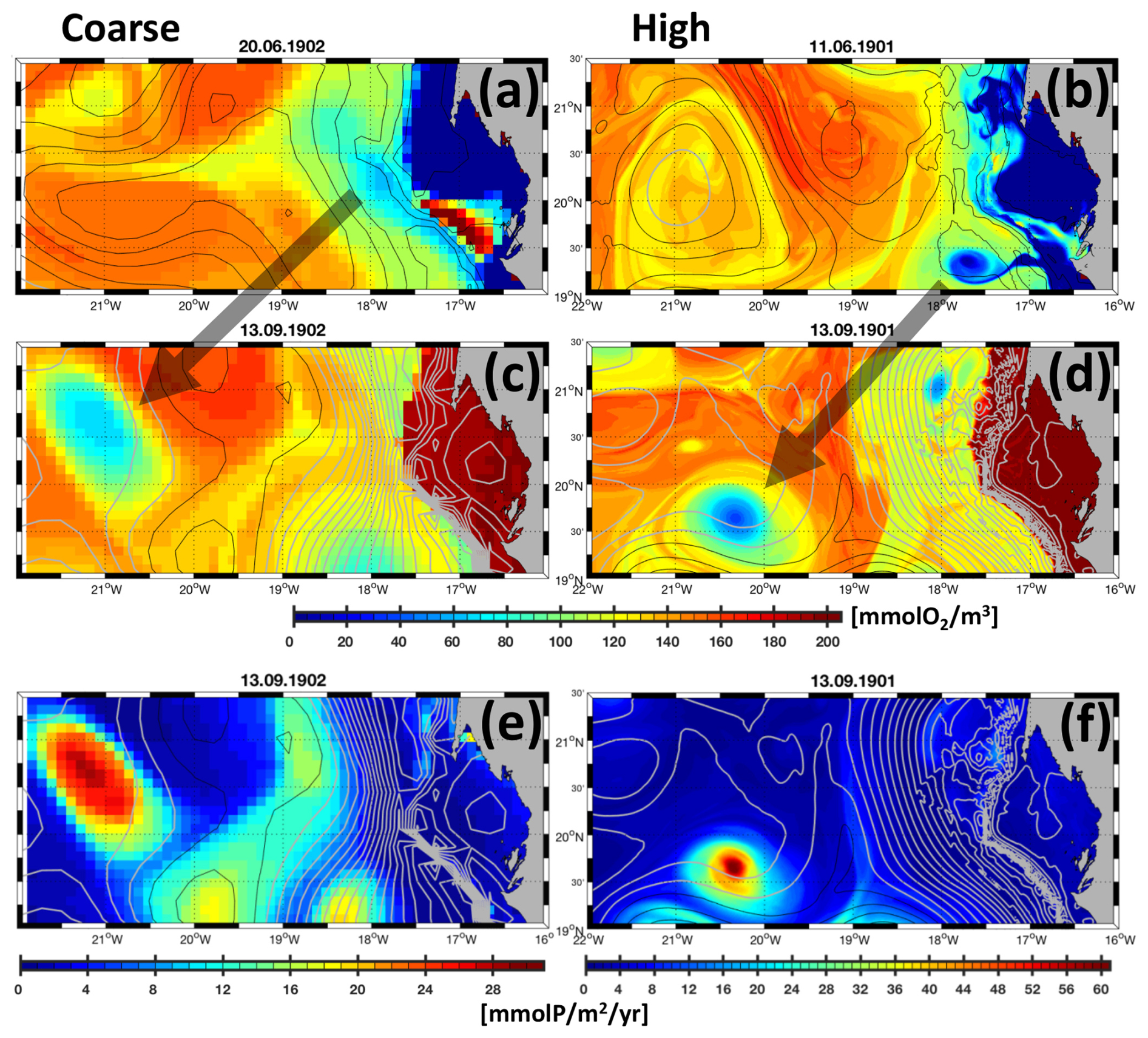
Figure A5 Simulated spawning and westward progression of a hypoxic anticyclonic mode water eddy (ACME). Panels (a), (c) and (e) refer to the Coarse configuration, while panels (b), (d) and (f) refer to the High configuration. The colors in panels (a)–(d) denote the minimum oxygen concentrations found locally in vertical water columns. Panels (e) and (f) show color-coded export production. Gray and black contours denote positive and negative sea surface height anomalies spaced at 2 cm. Panels (a) and (b) feature the ACME spawning in June as simulated with Coarse and High, respectively. The gray arrows pointing into panels (c) and (d) indicate the ACMEs' westward progression until September simulated with Coarse and High, respectively. Panels (e) and (f) show export production calculated as net biotic phosphate sources and sinks integrated over the upper 150 m water column in September from Coarse and High, respectively. The respective maximum export production coincides with the position of the ACMEs.

The upwelling season ends in July south of Cap Blanc (Mittelstaedt, 1991, their Fig. 4) when the winds weaken and veer into a more onshore direction driving currents that flush the shelf with oxygenated water of offshore origin (ould Dedah, 1993). The oxygen on the shelf is then replenished until the cycle restarts in spring. Figure A5e and f show that the ACMEs are associated with a biotic export production that is elevated relative to ambient waters in our simulations. Even so, both configurations retain rather constant oxygen concentrations within the ACMEs' cores. We conclude that the High and Coarse configurations simulate a series of complex coupled ocean circulation biogeochemical processes driving the evolution of oxygen in ACMEs in a surprisingly similar manner. Apparently, the differences among the configurations are limited to details rather than to materially different processes and dynamics.

Appendix B: Boundary conditions

The model configurations used in this study are peculiar in that the northern, southern and western boundaries are closed walls rather than a realistic representation of the polar gyre, the equatorial current system and the coast of America, respectively. Appendix B provides information as to how this may affect the model results in the high-resolution model domain. By introducing an artificial tracer into Coarse configuration that is continuously reset to zero at these boundaries and counts up time elsewhere, we count the time elapsed since water parcels have been in contact with the boundaries. After an integration of 30 years, we find that water in the 100 to 400 m depth interval entering the high-resolution model domain is older than 3 years (Fig. B1). This suggests that our findings at the end of our 3-year simulation are rather unaffected by our simple representation of boundaries.

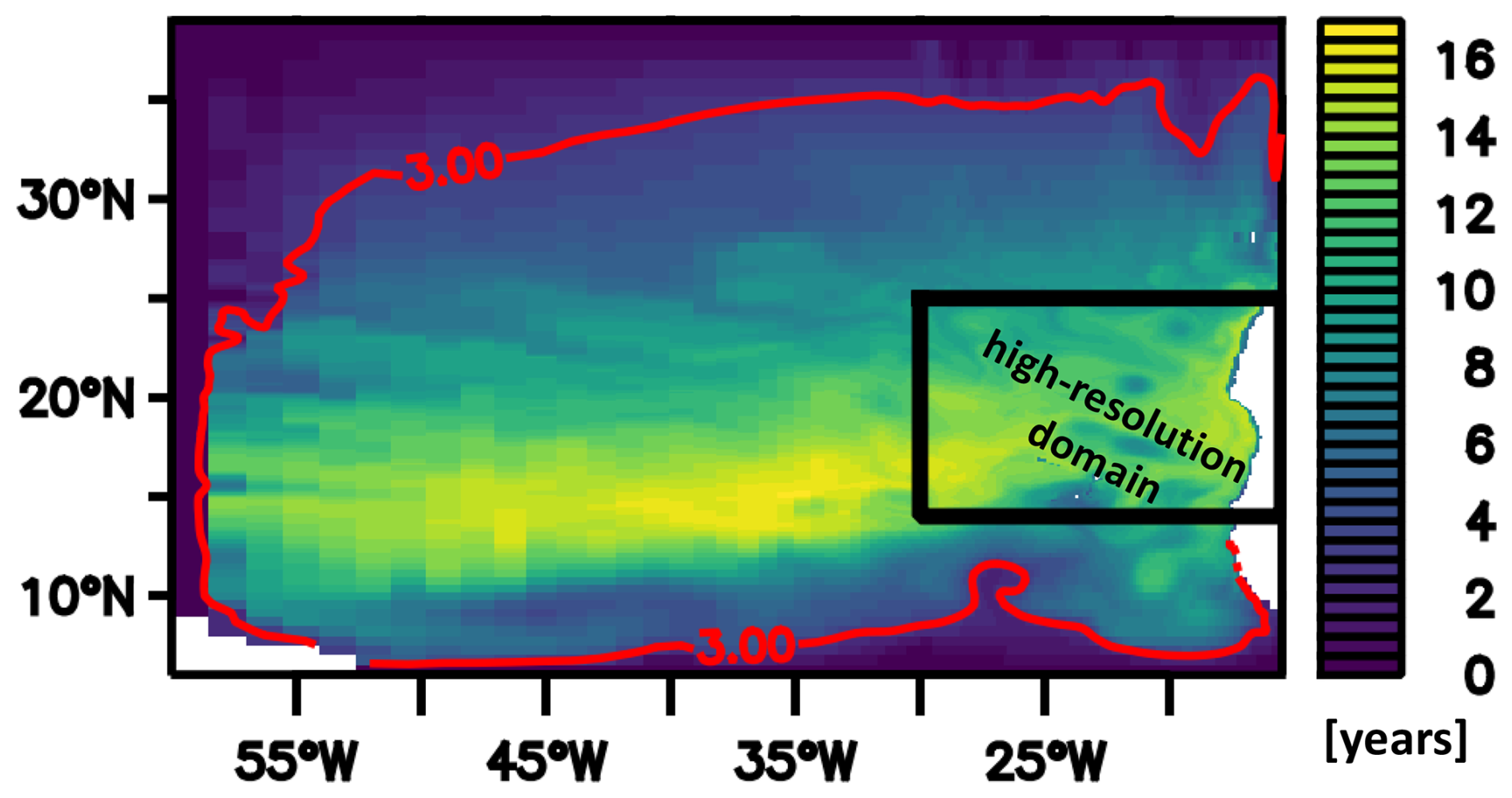
Figure B1 Simulated time elapsed since water parcels have been in contact with the northern, southern or western boundary of the model domain (monthly mean at the end of a 30-year integration of the Coarse configuration). The shown values for elapsed time are averaged over the 100 to 400 m depth interval. The red contour depicts the 3-year isoline, indicating that the contoured region is relatively undisturbed by boundary effects at the end of a 3-year simulation.