Eddy-covariance fluxes of CO₂, CH₄ and N₂O in a drained peatland forest after clear-cutting

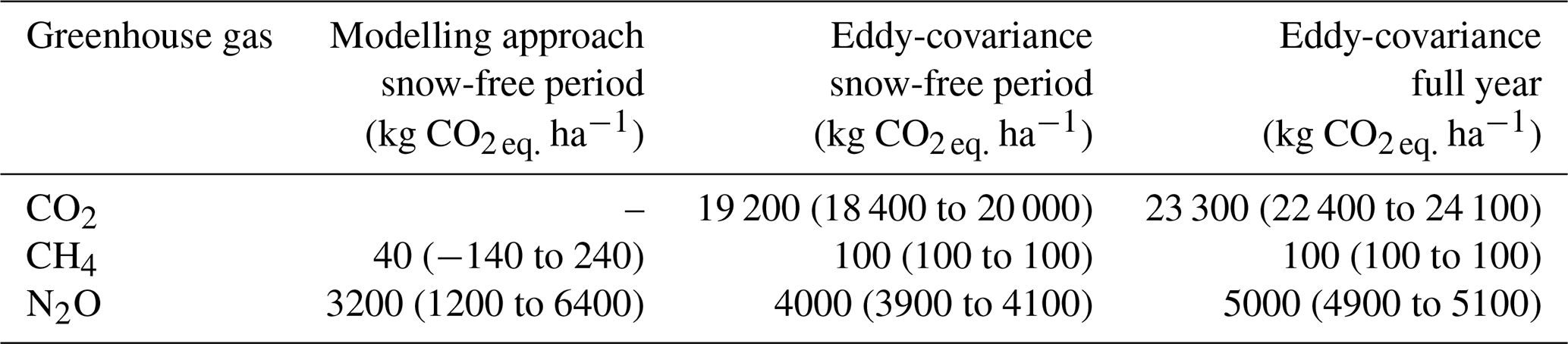
Rotation forestry based on clear-cut harvesting, site preparation, planting and intermediate thinnings is currently the dominant management approach in Fennoscandia. However, understanding of the greenhouse gas (GHG) emissions following clear-cutting remains limited, particularly in drained peatland forests. In this study, we report eddy-covariance-based (EC-based) net emissions of carbon dioxide (CO₂), methane (CH₄) and nitrous oxide (N₂O) from a fertile drained boreal peatland forest 1 year after wood harvest. Our results show that, at an annual scale, the site was a net CO₂ source. The CO₂ emissions dominate the total annual GHG balance (23.3 t CO_2 eq. ha⁻¹ yr⁻¹, 22.4–24.1 t CO_2 eq. ha⁻¹ yr⁻¹, depending on the EC gap-filling method; 82.0 % of the total), while the role of N₂O emissions (5.0 t CO_2 eq. ha⁻¹ yr⁻¹, 4.9–5.1 t CO_2 eq. ha⁻¹ yr⁻¹; 17.6 %) was also significant. The site was a weak CH₄ source (0.1 t CO_2 eq. ha⁻¹ yr⁻¹, 0.1–0.1 t CO_2 eq. ha⁻¹ yr⁻¹; 0.4 %). A statistical model was developed to estimate surface-type-specific CH₄ and N₂O emissions. The model was based on the air temperature, soil moisture and contribution of specific surface types within the EC flux footprint. The surface types were classified using unoccupied aerial vehicle (UAV) spectral imaging and machine learning. Based on the statistical models, the highest surface-type-specific CH₄ emissions occurred from plant-covered ditches and exposed peat, while the surfaces dominated by living trees, dead wood, litter and exposed peat were the main contributors to N₂O emissions. Our study provides new insights into how CH₄ and N₂O fluxes are affected by surface-type variation across clear-cutting areas in forested boreal peatlands. Our findings highlight the need to integrate surface-type-specific flux modelling, EC-based data and chamber-based flux measurements to comprehend the GHG emissions following clear-cutting and regeneration. The results also strengthen the accumulated evidence that recently clear-cut peatland forests are significant GHG sources.

1 Introduction

Globally, peatland soils store 650 000 Mt of carbon (C), which is equivalent to more than half of the C in the atmosphere (FAO, 2020). In Europe, the estimated peatland C stock is 43 620 Mt C, with a total peatland area of 58.8 Mha, 46 % of which is drained (UNEP, 2022). Drainage lowers the water table depth (WTD) and accelerates aerobic peat decomposition, resulting in carbon dioxide (CO₂) emissions and an annual loss of soil C stock equivalent to 160 Mt C (UNEP, 2022). In the specific context of Finland, the greenhouse gas (GHG) flux balance in forested peatlands has been quantified at both the stand level (Korkiakoski et al., 2023; Mäkiranta et al., 2010; Ojanen et al., 2010) and the national scale (Alm et al., 2023; Statistics Finland, 2022). However, the short-term impact of clear-cutting and subsequent site preparation on the GHG fluxes of forested peatlands remains unclear and is not currently included in the national GHG inventories. Therefore, estimates of the current GHG balance of forested peatlands under management are associated with a considerable degree of uncertainty.

Rotation forestry is currently the dominant forest management method in Fennoscandia,. It is characterized by forest stands with an even age structure, resulting from forest regeneration by clear-cutting and, later, from intermediate thinnings from below (Kuuluvainen et al., 2012). In Finland, 4.7 Mha of peatlands have been drained for forestry purposes (Korhonen et al., 2021). A large fraction of fertile drained peatland forests is currently at the mature stage and approaching a decision with respect to final harvesting and regeneration (Lehtonen et al., 2023). In rotation-based peatland forestry, clear-cutting typically leads to maintenance ditching to ensure adequate drainage for undisturbed tree growth (Päivänen and Hånell, 2012). However, rotation forestry that involves clear-cutting and maintenance ditching has been found to have several short-term negative external effects (Nieminen et al., 2018); these include increases in nutrient and dissolved organic carbon (DOC) exports to watercourses (Palviainen et al., 2022), loss of biodiversity (Paillet et al., 2010; Rajakallio et al., 2021), and enhanced CO₂ emissions (Korkiakoski et al., 2023). The magnitude and duration of the major GHG emissions – CO₂, methane (CH₄) and nitrous oxide (N₂O) – on drained forested boreal peatlands after clear-cutting remain largely unclear. This is because there have been only a few studies assessing them to date (Korkiakoski et al., 2019, 2023; Mäkiranta et al., 2010; Tong et al., 2022). The lack of information on how clear-cutting affects GHG emissions in drained boreal peatlands for forestry prevents the comparisons of climate change impacts of business-as-usual forestry (i.e. rotation) and alternative forest management methods (e.g. continuous cover forestry) (Kaarakka et al., 2021; Mäkipää et al., 2023).

Tree removal alters the local microclimate of forested peatlands by changing factors such as the amount of radiation available on the ground (Tikkasalo et al., 2024). This can result in higher soil temperatures (Pumpanen et al., 2004; Wu et al., 2011), potentially increasing peat decomposition and CO₂ emission rates (Jandl et al., 2007). On the other hand, piles of harvest residues may decrease the soil temperature, creating biotic and abiotic variation. Under drained or unsaturated moisture conditions, this process may be further enhanced due to increased oxygen availability in soil (Maljanen et al., 2010; Ojanen et al., 2013; Drzymulska, 2016). The harvest of trees in peatland forests raise the WTD by decreasing transpiration and interception (Sarkkola et al., 2010; Leppä et al., 2020a, b). This, in turn, may result in a slower peat decomposition rate. Furthermore, the removal of trees and decline in forest floor vegetation will lead to a strong immediate reduction in photosynthesis in clear-cutting areas. Drainage can increase root aeration and nutrient availability, which may benefit the rapid establishment of initial forest floor vegetation and tree seedlings (Mäkiranta et al., 2010) and enhance rates of ground vegetation carbon sequestration (Minkkinen et al., 2001). However, ground vegetation is insufficient to compensate for the increase in ecosystem respiration caused by the decomposition of logging residues (Mäkiranta et al., 2012; Ojanen et al., 2017; Korkiakoski et al., 2019; Tong et al., 2022). Consequently, clear-cutting transforms forested peatland ecosystems into net CO₂ sources during the early stages of stand development (Mäkiranta et al., 2010; Tong et al., 2022; Korkiakoski et al., 2023).

Drained peatland has decreased CH₄ emissions compared with pristine peatlands, due to improved soil aeration (Maljanen et al., 2010; Ojanen et al., 2010). After tree removal, the WTD typically rises (Korkiakoski et al., 2019; Leppä et al., 2020a), which supports the production of CH₄ in the extended anaerobic zone. This can turn peatland sites from net CH₄ sinks into sources (Korkiakoski et al., 2019). However, Ojanen et al. (2010, 2013) found that CH₄ emissions only increase when the WTD is at a shallow level (i.e. within 30 cm of the soil surface). Furthermore, the response of vegetation to drainage may affect the supply of substrate to methanogens (Minkkinen and Laine, 2006), which can further enhance or offset the hydrological effects of drainage on CH₄ fluxes.

Clear-cutting not only affects C fluxes but also leads to increased N₂O emissions (Robertson et al., 1987; Huttunen et al., 2003; Saari et al., 2009; Neill et al., 2006; Korkiakoski et al., 2019). This is due to the flush of decomposing logging residues and reduced nitrogen (N) uptake due to lower plant biomass, which both increase available soil N in the first years following harvest (Mäkiranta et al., 2012). N₂O production is also favoured by redox conditions that vary between oxidative and reductive, which exist in wet but unsaturated peat after clear-cutting and drainage. The production of N₂O responds to changes in soil moisture, so the effect of drainage on N₂O emissions is likely to depend on the combination of WTD change and soil nutrient status (Tong et al., 2022). Additionally, drying–rewetting events occurring during the growing season have been identified as “hot moments” for N₂O emissions (Groffman et al., 2009). Nevertheless, the accurate estimation of N₂O emissions has remained a significant challenge due to their considerable spatiotemporal variations (Rautakoski et al., 2024), which are a consequence of the inherent complexity of the various interacting processes. Furthermore, given that N₂O is a potent long-lived GHG and a stratospheric ozone-depleting substance that has been accumulating rapidly in the atmosphere over the last decades (Tian et al., 2024), it is important to determine the role of clear-cutting in regulating the global GHG budget.

Most studies on GHG fluxes in drained forested boreal peatlands after clear-cutting are based on manual chamber measurements (e.g. Mäkiranta et al., 2010; Tong et al., 2022). However, the magnitude and controls on CO₂, CH₄ and N₂O fluxes in these high-latitude northern ecosystems remain highly uncertain. This is mainly related to the poor spatial and temporal representation of manual chamber-based GHG measurements (Savage and Davidson, 2003). Clear-cutting creates a highly heterogeneous surface, which makes it challenging to interpret ecosystem GHG fluxes due to variation in surface-specific fluxes. Previous research has demonstrated that forest floor vegetation heterogeneity, logging residues and ditches cause significant spatial variability in GHG fluxes from drained peatlands and clear-cut areas (Minkkinen and Laine, 2006; Ojanen et al., 2010; Mäkiranta et al., 2012; Rissanen et al., 2023). In this context, eddy covariance (EC) has become a widely used technique for measuring the GHG exchange (Baldocchi, 2003) due to its ability to provide high-temporal-resolution exchange rates integrated over a relatively large area. The EC footprint (i.e. the source area of the measured flux) collects the contributions of each element of the surface area to the measured vertical turbulent flux (Vesala et al., 2008). Therefore, this area could be divided into distinct surface types that form a heterogeneous matrix, enabling direct assessments of each surface type on the measured GHG fluxes. While studies attributing EC-measured surface fluxes to specific surface types at heterogeneous ecosystems exist (Forbrich et al., 2011; Franz et al., 2016; Tuovinen et al., 2019; Ludwig et al., 2024), none of them focus on heterogeneous clear-cut areas. The likely reason for this is the lack of high-resolution data on surface types within the EC tower's footprint. However, the use of high-resolution georeferenced imagery from unoccupied aerial vehicle (UAV) surveys (and the possibility to derive detailed surface maps) now enables the integration of footprint models and GHG flux measurements as well as the attribution of measured fluxes to specific surface features.

In light of the preceding considerations, there is a considerable degree of uncertainty associated with the magnitude of GHGs as well as their key modulating processes and spatial and temporal heterogeneity on drained boreal peatland forests under forestry management. This deficiency is directly attributable to the paucity of available studies on the subject. It is, therefore, imperative to improve our understanding of the impact of clear-cutting and different surface types on GHG fluxes. Here, we examined the CO₂, CH₄ and N₂O fluxes from a fertile drained boreal peatland forest located in Southern Finland during the first full year (second growing season) after clear-cutting. GHG fluxes were measured using an EC system during the year 2022, while clear-cutting was conducted during the winter and spring 2021. Information on surface-type variation across the footprint area was collected via drone imaging in June 2022. Our specific aims were as follows:

1. quantification of the magnitude and temporal variation in CO₂, CH₄ and N₂O fluxes along their annual balances.

2. estimation of the differences in surface-type-specific CH₄ and N₂O fluxes, as well as sensitivity of the fluxes to environmental variation.

2 Materials and methods

2.1 Measurement site

The Ränskälänkorpi study site is a boreal peatland forest (ca. 24 ha) located in southern Finland (61°11^′ N, 25°16^′ E; 144 m a.s.l.; Figs. 1, S1) that was drained for forestry before the 1960s. The climate is humid continental with a 30-year (1981–2022) mean annual air temperature and precipitation sum of 4.2 °C and 611 mm, respectively. Air temperature and precipitation were obtained from a 10 km × 10 km grid of daily weather data from the Finnish Meteorological Institute (FMI) resulting from a kriging-interpolation procedure (Venäläinen and Heikinheimo, 2002). On average, the site maintains snow cover for 133 d, typically from early November to late April. The forest is dominated by Norway spruce (Picea abies (L.) Karst.; about 70 % of all trees), with some Scots pine (Pinus sylvestris L.) and Downy birch (Betula pubescens Ehrh.). The forest floor vegetation is sparse and consists of mosses (mainly Hylocomium splendens, Pleurozium schreberi and Dicranum polysetum), dwarf shrubs (mainly Vaccinium myrtillus and Vaccinium vitis-idaea) and forbs (such as Dryopteris carthusiana, Gymnocarpium dryopteris, Lysimachia europaea and Oxalis acetosella). The site consists of sedge–wood-dominated peat, which is generally more than 1 m deep. The site is a fertile and well-drained, dominated by Norway spruce, and represents mainly nutrient-rich and herb-rich (Rhtkg II) and Vaccinium myrtillus (Mtkg II) site types according to the Finnish site types for drained peatland forests (Laine et al., 2012). In March 2021, the site was divided into three areas with different harvest treatments: non-harvested control (ca. 7.3 ha), selection harvest (continuous cover forestry – CCF; ca. 10.0 ha) and clear-cutting (CC; ca. 6.1 ha). The harvesting in the CCF and CC areas took place with harvester machinery primarily from 18 March to 1 April 2021, when the soil was frozen. Harvesting was completed in June 2021 in the north-western section of the CC area. This study was conducted in the CC area, where all the trees were cut. Some large, dead trees were retained on the site, and the resulting logging residue (i.e. foliage, branches and stumps) was left on the ground. The understory vegetation was significantly impacted by the disturbance caused by the harvester and logging machines. The mean peat soil $\mathrm{C}/\mathrm{N}$ ratio across 0–20 cm depth at the CC area was 32.1 ± 4.7 (C % = 54.8 ± 1.5 and N % = 1.7 ± 0.2; n=6 sampling locations). The WTD relative to the peat surface during the 2022 growing season ranged from −9 to −64 cm, with an average value of −28 ± 9 cm (n=8 sampling locations). The stand regeneration was carried out in summer 2021 through ditch mounding and planting of Norway spruce seedlings, with an approximate density of 1800–2000 seedlings ha⁻¹. The harvest and regeneration are according to common practices for operational forestry in Finland.

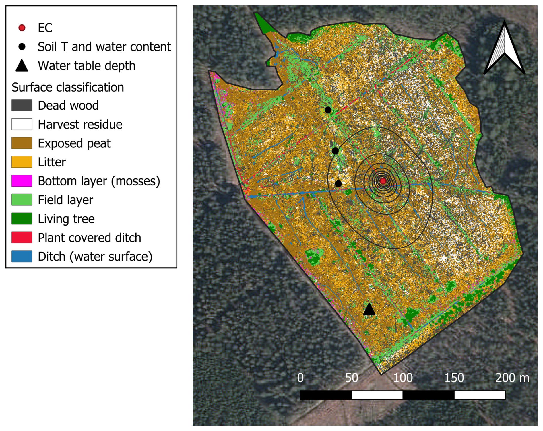
Figure 1 Surface-type classification and aerial view of the experimental set-up in the clear-cut area. The black triangle shows the location of the water table depth measurement, black circles show the location of the soil temperature and moisture sensors, and the red circle shows the location of the eddy-covariance (EC) tower. The contour lines display the mean footprint area (10th–90th percentiles) for the year 2022. The pixel colour indicates the surface type. The background aerial photo was acquired from the National Land Survey of Finland Topographic Database (retrieved June 2024 and distributed under a CC-BY 4.0 licence).

2.2 EC measurements

Ecosystem–atmosphere greenhouse gas exchange was measured from a 3.1 m tall tower in the middle of the CC area using the EC technique (see Fig. 1). The distance from the tower to the forest edge was at least 100 m in all directions. High-frequency data on the three wind components and sonic temperature were acquired with an ultrasonic anemometer (uSonic-3 Cage MP, METEK GmbH, Germany), CO₂ and water vapour (H₂O) mixing ratios were obtained with a nondispersive infrared sensor (LI-7200RS, LI-COR Biosciences, NE, USA), and CH₄ and N₂O mixing ratios were acquired with a tunable infrared laser direct-absorption spectrometer (TILDAS, Aerodyne Research Inc., USA). All of the EC data were logged with a 10 Hz frequency. TILDAS data were logged to separate files and combined with the other EC data during data post-processing. The TILDAS was located in a small, air-conditioned measurement hut and sampled the air with a 9 m long heated Teflon tube. Rapid flow in the tube was created with a scroll pump (TriScroll 600, Agilent Technologies Inc., USA). The LI-7200RS was situated in the measurement tower and sampled the air with a heated sampling tube distributed with the instrument (ca. 0.7 m long tube with a 5.3 mm inner diameter) and pump. The gas analysers sampling inlets were located next to the sonic anemometer (0.18 m horizontal separation).

In addition to the EC fluxes, several environmental variables were continuously monitored at the EC station. These include photosynthetically active radiation (PAR; LI-190R Quantum Sensor, LI-COR Biosciences, USA), air temperature (T_air) and humidity (HMP155 humidity and temperature probe, Vaisala Oyj, Finland), the shortwave and longwave incoming and outgoing radiation component (CNR4 four-component net radiometer, Kipp & Zonen, the Netherlands), precipitation (P; TR-525M rainfall sensor, Texas Electronics, USA), soil temperature (T_soil), and water content (θ) at 10 cm depth (HydraProbe II, Stevens Water Monitoring Systems Inc., USA). These variables were logged at a 1 min time step. Soil temperature and water were also monitored at other locations at the clear-cut (see Fig. 1) with TMS-4 microclimate loggers (Standard datalogger, TOMST s.r.o, Prague, Czechia), and the water table depth was measured with an Odyssey Capacitance Water Level Logger (Dataflow Systems Ltd, New Zealand).

2.3 EC data processing

As much as was feasible, EC flux data processing followed international standards set, for example, by the Integrated Carbon Observation System (ICOS) network (Franz et al., 2018). Flux calculations were executed with the EddyPro open-source software (version 7.0.7, LI-COR Inc., USA). Fluxes were calculated using a 30 min averaging time, and turbulent fluctuations were separated from the measurements using block-averaging. The high-frequency time series were despiked following Mauder et al. (2013). High-frequency gas data had already been converted to dry mixing ratios internally by the measurement devices (LI-7200RS and TILDAS); hence, no conversions were done during post-processing. The gas sampling system (tubes and filters) induced time lags between wind and gas mixing ratio data. These time lags were estimated using cross-covariance maximization and were accounted for before flux calculations. Furthermore, the flow coordinates were rotated using sector-wise planar fitting (Rannik et al., 2020) before calculating the covariances (i.e. fluxes) between the vertical wind component and gas mixing ratio time series. EC fluxes are always underestimated due to high-frequency and low-frequency dampening of the signal caused by the measurement system (e.g. dampening of the gas fluctuations in the sampling lines) and the need to use a finite flux averaging time, respectively. In this study, the underestimation of gas fluxes was corrected following the approach by Fratini et al. (2012) and Moncrieff et al. (2005) with the exception that the cut-off frequencies characterizing the high-frequency dampening of each gas signal were estimated based on cospectra between vertical wind and gas time series and not from gas power spectra following Peltola et al. (2021).

The fully processed gas flux time series resulting from the processing procedure described above were quality filtered following Vitale et al. (2020) with few differences. First, flux data were discarded if the flux values were outside predefined limits, instrument diagnostics signalled erroneous measurement or site diaries suggested disturbance to the data. Then, the procedure by Vitale et al. (2020) was followed with the exception that the statistical model used in the quality filtering procedure was estimated using singular spectrum analysis and low-rank reconstruction of the time series (Golyandina et al., 2001; Mahecha et al., 2007), instead of the multiplicative model used in Vitale et al. (2020). After quality filtering, low-turbulence periods during which EC fluxes did not represent surface–atmosphere exchange were identified using friction velocity, and periods during which the friction velocity was below a site-specific threshold (0.09 m s⁻¹) were removed from further analysis. After this procedure, the flux data coverage was 64 %, 57 % and 57 % for CO₂, CH₄ and N₂O flux time series, respectively, with the majority of the data gaps occurring during low-wind nights.

For calculating daily mean fluxes or annual GHG balances, the gaps in flux time series needed to be filled. The gaps were filled separately with three machine learning (ML) algorithms: random forest (RF), extreme gradient boosting (XGB) and k-nearest neighbours (kNN). These three algorithms were selected based on their good performance with respect to filling gaps in flux time series in prior studies (e.g. Goodrich et al., 2021; Irvin et al., 2021; Vekuri et al., 2023). The ensemble median of the three gap-filled time series was then used to estimate annual GHG balances and daily fluxes, whereas the spread between the three estimates was used to evaluate the range of plausible annual GHG balance values. This approach minimizes the uncertainty in annual balances that would otherwise result from the selection of a particular algorithm for gap filling. However, it is possible that the spread may underestimate the total uncertainty in the annual fluxes, as it does not take into account, for example, the contribution of the random uncertainty associated with EC observations, and it relates only to uncertainty associated with the gap-filling process. The “xgboost” (version 1.7.1) Python package was used for the XGB method, whereas the “RandomForestRegressor” and “KNeighborsRegressor” “scikit-learn” (version 1.1.1) functions were utilized in the RF and kNN methods, respectively. ML model training and testing of predictive performance were executed as follows. First, model hyperparameters were tuned against a random subset of data with the “RandomizedSearchCV” scikit-learn function. After hyperparameter tuning, artificial gaps (covering 15 % of the data) were introduced in random locations in the flux time series, and the lengths of these gaps were drawn from a distribution describing the length of actual gaps in the time series (Irvin et al., 2021). Measured data from these gaps were used as independent test data, whereas all of the other data were used in model training. The trained model predictive performance was then evaluated against the test data, and this training–testing procedure was executed independently five times. The final models used in gap filling the flux time series were trained using all of the measured data. The following predictors were used in this gap-filling procedure for CH₄ fluxes: normalized daily incoming potential solar radiation (RPOT) and its first time derivative; T_air and its average during the past 3 h, 1 and 7 d; incoming shortwave radiation; surface temperature calculated from upwelling longwave radiation; vapour pressure deficit; sine- and cosine-transformed wind direction; and T_soil. The list of predictors was the same for N₂O fluxes except that the soil water content (θ) was also included. For CO₂ flux time series gap filling, the same predictors were used as for CH₄, but the daily normalized RPOT and its first time derivative (values ranged between zero and one within each day) were also included so that the models better captured the CO₂ flux daily cycle. For kNN, data were normalized to zero mean and unit variance, whereas for RF and XGB data were not normalized. The predictive performance (R²) of the ensemble models obtained with this procedure was 0.75±0.04 (mean ± standard deviation of the five predictions), 0.66±0.05 and 0.92±0.01 for the CO₂, CH₄ and N₂O fluxes, respectively; the slopes of the linear fits between the predictions and observations were 0.97±0.08, 1.01±0.02 and 1.01±0.04, respectively; and the intercepts were 0.01±0.07 µmol m⁻² s⁻¹, $-\mathrm{0.01}\pm \mathrm{0.04}$ nmol m⁻² s⁻¹ and $-\mathrm{0.02}\pm \mathrm{0.04}$ nmol m⁻² s⁻¹, respectively. These results for the predictive performance differ from some of the aforementioned studies; however, this is likely due to the nature of variability in these fluxes at our site (low photosynthesis and CO₂ flux variability, marked seasonal variability in N₂O fluxes, and low CH₄ fluxes; see Sect. 3.1).

CO₂ fluxes (net ecosystem exchange, NEE; with a positive sign denoting net emissions) were decomposed to ecosystem respiration (R_eco) and gross primary productivity (GPP) following the nighttime decomposition method by Reichstein et al. (2005) with the slight modifications by Wutzler et al. (2018). However, in contrast to Reichstein et al. (2005), we forced nighttime GPP to zero by subtracting the 1.5 d running median of the nighttime GPP from the GPP time series (and added it to the R_eco time series) and forced any residual nighttime GPP to zero. This way, $\mathrm{NEE}=R_{\mathrm{eco}}-\mathrm{GPP}$ is valid at all time steps and GPP is zero when there is no incoming solar radiation.

2.4 EC flux footprint

Turbulent fluxes measured with EC relate to the surface fluxes via

$$\begin{array}{}\text{(1)}& F\left(t\right)=\int \int \mathit{\phi }(x,y,t)f(x,y,t)\mathrm{d}x\mathrm{d}y,\end{array}$$

where F=F(t) is the flux measured with EC at time t; f=f(xyt) is the surface flux at location (xy) at time t; and φ=φ(xyt) is so-called footprint function, which describes the source area of EC flux measurements (Vesala et al., 2008). The footprint gives an estimate of the relative contribution of each location on the surface to the measured turbulent flux, and it is possible link surface features to measured fluxes using such information. If we assume constant fluxes (f_j(t)) from surface-type j during time step t, Eq. (1) can be simplified as

$$\begin{array}{}\text{(2)}& F\left(t\right)\approx \sum _j{\mathit{\phi }}_j\left(t\right)f_j\left(t\right),\end{array}$$

where φ_j is the overall contribution of surface-type j to the EC flux source area during time step t.

In this study, the source area, i.e. footprint, for the measured gas fluxes was estimated for each 30 min period with the Kljun et al. (2015) model, which is a simple two-dimensional analytical parameterization of results obtained with a backward Lagrangian stochastic particle dispersion model (Kljun et al., 2002). The model requires information on the flow, namely, the wind speed, boundary layer height, Obukhov length, standard deviation of lateral velocity fluctuations, friction velocity and wind direction for rotating the footprint to the prevailing direction. All of these were measured with the EC equipment, except boundary layer height, which was retrieved from the ERA5 reanalysis product (Hersbach et al., 2023). In addition to these measurements, footprint calculations require information on the EC measurement height (z), displacement height (d) and surface roughness length (z₀). The CC surface is a complex mosaic of different surface types and vegetation heights with small-scale topography. This variability influences the flow field above the surface, and this needs to be accounted for in footprint calculations. To resolve this issue, we opted to use varying values of d in the calculations and estimated them from the EC data via a logarithmic wind profile equation, similarly to the method used in Helbig et al. (2016), with the exception that only near-neutral periods were used in this analysis and that estimates of d were bin-averaged in the wind direction and 30 d bins before using them in the footprint calculations to reduce the noise stemming from the uncertain calculation procedure. The estimated values for d ranged between 0.8 and 2.0 m (5th–95th quantiles of the estimates) during the study period (Fig. S2). z₀ was implicitly included in the footprint calculations via the ratio between wind speed and friction velocity (Kljun et al., 2015). With this footprint estimation procedure, we accounted for the effect of temporally and spatially varying surface characteristics on the footprints.

2.5 Drone imaging

An orthomosaic of the CC area was generated using drone images captured on 8 June 2022 between 12:00 and 14:00 LT (UTC+3) with a DJI Matrice 210 V2 drone equipped with a Zenmuse X7 sensor for RGB and a Micasense Altum sensor for multispectral images. The flight altitude was 75 m, and images were captured with 95 % frontlap and 85 % sidelap. The weather conditions were cloudy throughout the flight, providing even spectral conditions. The images were georeferenced with 10 ground control points measured with a Trimble R12 GNSS device and processed into an orthomosaic and digital elevation model (DEM) using Agisoft Metashape 1.7.3. The resulting RGB orthomosaic had a ground sample distance (GSD) of 1.16 cm and a multispectral orthomosaic of 3.23 cm

2.6 Surface-type classification

The land surface classification is based on a geographical-object-based image classification approach similar to De Luca et al. (2019) and was executed using the drone images (see Sect. 2.5). Orthomosaics from the CC area including RGB, red edge (RE) and near-infrared (NIR) channels were merged with the DEM and segmented by spectral signal Euclidian distance using the “LargeScaleMeanShift” (LSMS) segmentation module found in the Orfeo ToolBox (Grizonnet et al., 2017). Parameters for LSMS were spatialr = 1, ranger = 5 and minsize = 40. The LSMS segmentation resulted in 1.4 million polygons, enabling detailed segmentation of surface cover elements down to ca. 10 cm × 10 cm in size.

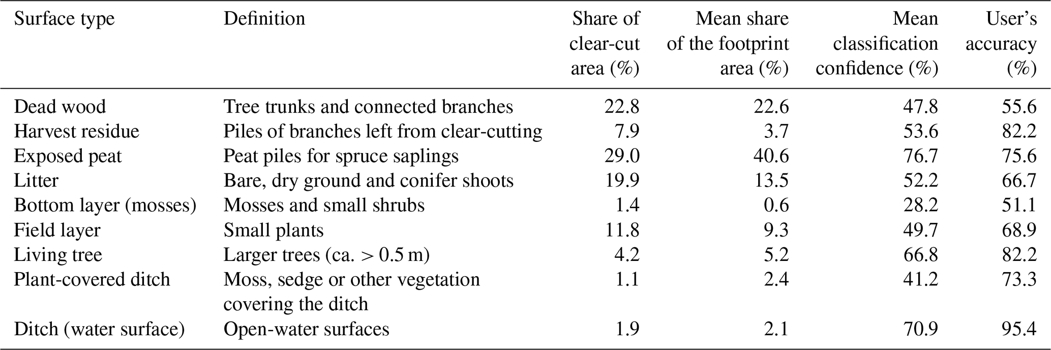
To classify the segments, training data consisting of samples of different surface types were used to train the random forest classifier within the Orfeo ToolBox using the means and variances of the R, G, B, RE, NIR and DEM channels inside the polygon. Random forest uses multiple decision trees trained on bootstrap sets of training data, and the classification is based on the majority vote of the decision trees (Breiman, 2001). The training data were manually labelled on the segmented polygon in QGIS software using the RGB image and field surveys. The training data covered 0.27 % of the CC area and included even numbers of samples for each surface type distributed evenly across the surveyed area to account for small spectral changes due to slight changes in the cloud optical depth during the flight. The classes (Table 1; Figs. 1, S3) were selected by prior field surveys to be a representative set of different surface types that could accurately be distinguished from the drone orthomosaic and were readily identifiable in situ. With the trained model, the rest of the segments were classified into different land cover types with a mean balanced accuracy of 81.2 % and Cohen's kappa coefficient of 0.64. As the number of segments in the different surface types varies widely, Table 1 shows also the user's accuracy for class samples. Piles of harvest residue and dead wood are common throughout the area, and the difference between those classes is difficult to distinguish in many cases, possibly resulting in a mixed classification. A moderate amount of precipitation occurred just before the flight, but this did not affect the classification of exposed peat, despite the presence of small ponds in the depressions. The plant-covered ditches, however, can be classified as the bottom or the field layer in some cases.

Table 1 Surface-type classification. Names of the surface types, their definition, share of the clear-cut area and average footprint area, mean classification confidence level (share of votes for the majority class) of the random forest classifier, and the user's accuracy (share of correctly classified segments from the classification) for an equal-sized sample of each class.

2.7 Correlation analysis

To understand which environmental parameters should be included in the statistical flux models, we quantified the GHG flux correlation with environmental variables with the bivariate Spearman rank correlation coefficient (r_s). r_s was calculated for the 30 min, non-gap-filled time series (except for GPP) by omitting the 30 min intervals that did not have observations recorded. For CO₂ flux, we present both the NEE ($F_{{\mathrm{CO}}_{\mathrm{2}}}$) and GPP, as the NEE consists of two components (GPP and R_eco). The environmental variables are precipitation (P), PAR, water content in air ($w_{{\mathrm{H}}_{\mathrm{2}}\mathrm{O}}$), WTD, air and soil temperature (T_air and T_soil, respectively), and soil water content (θ). T_air, P, $w_{{\mathrm{H}}_{\mathrm{2}}\mathrm{O}}$ and PAR are measured at the EC tower, and the locations of the T_soil, WTD and θ measurements are shown in Fig. 1.

2.8 Splitting CH₄ and N₂O flux into surface-type and environmental controls

We developed a statistical model that can capture the spatiotemporal variability in the fluxes, $F_{{\mathrm{CH}}_{\mathrm{4}}}$ and $F_{{\mathrm{N}}_{\mathrm{2}}\mathrm{O}}$. We included the surface-type (ST; Table 1) temperature and soil water availability effects in the model. Soil water availability was only included as a general term, without the ST-specific contribution. We opted to use only air temperature as the single independent ST-specific environmental variable in our model, as T_air can be expected to be uniform across the whole clear-cut area. The same assumption is more challenging to justify for soil temperature, soil moisture or WTD, which are influenced by soil processes and topography and expected to vary spatially within the study site.

Six alternative models were fitted to the EC flux measurements. The response variable in both models was the natural logarithm of observed fluxes, either CH₄ or N₂O. The first model (Eq. 3) is referred to as baseline model and assumes coherent responses of soil fluxes across the site. The second model (Eq. 4) is an extension of the baseline model and includes a soil moisture (θ) term. The second model is referred to as the baseline θ model. The third model (Eq. 5) is an ST-specific model and allows soil-cover-specific variation in fluxes (similar to Ludwig et al., 2024) and in their temperature responses. Models 4–6 are modifications of the third model. Model 4 (Eq. 6) does not have an ST-specific temperature term, model 5 (Eq. 7) includes a soil moisture term and model 6 (Eq. 8) is similar to model 5 but does not include the ST-specific temperature term. Models 3–6 (Eqs. 5–8) are named the “full”, “full no δ”, “full θ” and “full θ no δ” models, respectively.

$$\begin{array}{}\text{(3)}& {\displaystyle }\ln \left(F_i\right)=\mathit{\alpha }+\mathit{\beta }{\displaystyle \frac{T_{\mathrm{air},i}-T_{\mathrm{ref}}}{\mathrm{10}\mathrm{°}\mathrm{C}}}\text{(4)}& {\displaystyle }\ln \left(F_i\right)=\mathit{\alpha }+\mathit{\beta }{\displaystyle \frac{T_{\mathrm{air},i}-T_{\mathrm{ref}}}{\mathrm{10}\mathrm{°}\mathrm{C}}}+\mathit{\zeta }{\mathit{\theta }}_i\text{(5)}& {\displaystyle }\begin{array}{rl}\ln \left(F_i\right)& =\mathit{\alpha }+\mathit{\beta }{\displaystyle \frac{T_{\mathrm{air},i}-T_{\mathrm{ref}}}{\mathrm{10}\mathrm{°}\mathrm{C}}}\\ & +{\sum }_{j=\mathrm{1}}^N{\mathit{\phi }}_{i,j}\left({\mathit{\gamma }}_j+{\mathit{\delta }}_j{\displaystyle \frac{T_{\mathrm{air},i}-T_{\mathrm{ref}}}{{\mathrm{10}}^{\circ }C}}\right)\end{array}\text{(6)}& {\displaystyle }\ln \left(F_i\right)=\mathit{\alpha }+\mathit{\beta }{\displaystyle \frac{T_{\mathrm{air},i}-T_{\mathrm{ref}}}{\mathrm{10}\mathrm{°}\mathrm{C}}}+{\sum }_{j=\mathrm{1}}^N{\mathit{\phi }}_{i,j}{\mathit{\gamma }}_j\text{(7)}& {\displaystyle }\begin{array}{rl}\ln \left(F_i\right)& =\mathit{\alpha }+\mathit{\beta }{\displaystyle \frac{T_{\mathrm{air},i}-T_{\mathrm{ref}}}{\mathrm{10}\mathrm{°}\mathrm{C}}}+\mathit{\zeta }{\mathit{\theta }}_i\\ & +{\sum }_{j=\mathrm{1}}^N{\mathit{\phi }}_{i,j}\left({\mathit{\gamma }}_j+{\mathit{\delta }}_j{\displaystyle \frac{T_{\mathrm{air},i}-T_{\mathrm{ref}}}{\mathrm{10}\mathrm{°}\mathrm{C}}}\right)\end{array}\text{(8)}& {\displaystyle }\ln \left(F_i\right)=\mathit{\alpha }+\mathit{\beta }{\displaystyle \frac{T_{\mathrm{air},i}-T_{\mathrm{ref}}}{\mathrm{10}\mathrm{°}\mathrm{C}}}+\mathit{\zeta }{\mathit{\theta }}_i+{\sum }_{j=\mathrm{1}}^N{\mathit{\phi }}_{i,j}{\mathit{\gamma }}_j\end{array}$$

In the above expressions, F_i is the observed 30 min flux; α, β, γ, δ and ζ are free parameters to be estimated; φ_i,j is the fraction of surface-type j inside the footprint of observation i; T_ref=10 °C is the reference temperature; and θ is the mean soil moisture measured at the three locations shown in Fig. 1.

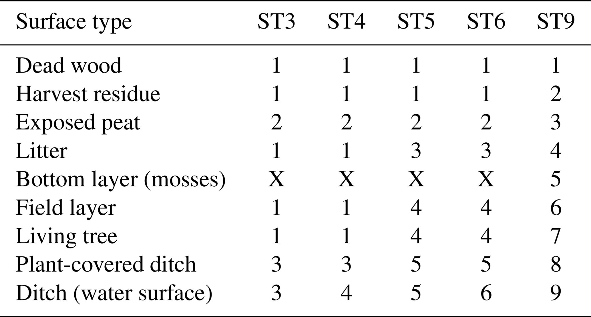
For the ST-specific models (Eqs. 5–8), we consider models with either 3, 4, 5, 6 or 9 surface types (ST3, ST4, ST5, ST6 and ST9, respectively), bringing the total number of models considered to 22 for both GHGs. ST9 considers all of the classified surface types. ST5 is built from ST9 by leaving out the bottom layer class (which covers only ca 0.6 % on average of the footprint areas) and by combining the dead wood and harvest residue classes, the ditch (water surface) and plant-covered ditch classes, and the living tree and field layer classes. Similarly, ST3 is built from ST5 by further combining all classes except the exposed peat class and the class containing both ditch types. ST4 and ST6 are derived from ST3 and ST5, respectively, by allotting the open ditches and plant-covered ditches to their own classes. The different surface-type combinations are summarized in Table 2 (see also Figs. 1 and S3 for a visualization of surface types in the CC area).

Table 2 Surface type combinations between ST-specific models. The table shows which surface types are combined in different ST-specific models. The same number in a column indicates that the surface types are combined. X indicates that the surface type is removed from the analysis.

The free parameters of the models, α, β, ζ, γ_j, δ_j and σ_ϵ (the standard deviation of the likelihood function), were estimated using Bayesian inference and Markov chain Monte Carlo (MCMC) methods with the “pyMC” package (Abril-Pla et al., 2023). The prior distribution of α and ζ was set to a normal distribution with a mean of 0 and a standard deviation of 2. The prior distribution of γ follows a hierarchical design: the prior for each surface type is normally distributed with mean μ_γ and standard deviation σ_γ, and the prior distribution for mean μ_γ was the standard normal distribution ${\mathit{\mu }}_{\mathit{\gamma }}\sim N(\mathrm{0},\mathrm{1})$. We used exponential distributions as priors for β and δ with rate parameters λ_β and λ_δ. We used a normally distributed likelihood function with a standard deviation σ_ϵ. We set the prior distribution for σ_ϵ to be an exponential distribution with a rate parameter λ_ϵ. Finally, the rate parameters λ_i of the exponential distributions for β, δ, σ_ϵ and σ_γ were set such that the full width at half maximum (FWHM) of the prior predictive distributions (Figs. S4, S5) was at least 2 times wider than the FWHM of the observed flux distributions. For simplicity, the same values were used for both GHGs: σ_γ=2.0 and ${\mathit{\lambda }}_l=\mathrm{1.0};l\in \mathit{\{}\mathit{\beta },\mathit{\delta },\mathit{ϵ}\mathit{\}}$. The parameters were estimated using the “pymc.sampling.mcmc.sample” function of the pyMC package with four chains, 2000 samples per chain and a tuning period of 2000 steps; i.e. a total of 8000 individual parameters sets were drawn for further analysis. All of the other sampler settings were left as default. The full, non-gap-filled, EC flux data sets were used in the parameter estimation; i.e. the artificial gaps introduced to the flux data sets for developing the gap-filling model were not present in this parameter estimation.

We evaluate the model performance based on the expected log posterior density of leave-one-out cross validation (ELPD-LOO). ELPD-LOO was calculated using the compare function of the “ArviZ” Python package, which uses the Pareto-smoothed importance sampling to refit the model parameters (Vehtari et al., 2017). The compare function ranks the models based on the expected log posterior density of the left out samples. While a single ELPD-LOO value is not easy to interpret in terms of model performance, models are straightforward to compare against each other, as a higher ELPD-LOO value marks better performance.

We defined Eqs. (3)–(8) on a natural logarithm (ln) base, as natural logarithm transformations of the measured flux values were normally distributed based on quantile–quantile plotting. When transforming the measured 30 min fluxes to a natural logarithm base, we omitted the CH₄ fluxes that were below −10 nmol m⁻² s⁻¹ and those N₂O values that were below 0 nmol m⁻² s⁻¹. We chose these limits because CH₄ fluxes varied randomly around zero during a low-flux period, whereas N₂O fluxes were clearly positive throughout the measurement period, with only occasional negative flux observations. The CH₄ flux values were then shifted by 10 nmol m⁻² s⁻¹ before the natural logarithm was applied. This shift was also accounted for when the model results were transformed back into units of nanomoles per square metre per second. Additionally, we accounted for a natural logarithm transformation bias when transforming the modelled fluxes to nanomoles per square metre per second. In total, the back transformation is as follows:

$$\begin{array}{}\text{(9)}& F_i=\exp \left(F_{i,\ln }+{\displaystyle \frac{{\mathit{\sigma }}_{\mathit{ϵ}}^{\mathrm{2}}}{\mathrm{2}}}\right)-S,\end{array}$$

where F_i,ln is the modelled flux in a natural logarithm base, σ_ϵ is the standard deviation of the likelihood function and S is the shift (S=0 nmol m⁻² s⁻¹ for N₂O and S=10 nmol m⁻² s⁻¹ for CH₄).

To further understand the GHG emissions from different surface types, we calculated the surface-type-specific fluxes by setting the contribution of each surface type to unity (${\mathit{\phi }}_{i,j}=\mathrm{1}$ in Eq. 4) in turn, while zeroing others. We calculated 8000 different flux values with the parameters estimated in the MCMC sampling.

3 Results

3.1 Ecosystem-scale greenhouse gas fluxes

The CC area at the Ränskälänkorpi study site was a strong net source of GHGs during the first full year (second growing season) after clear-cutting (Figs. 2, S6). The eddy-covariance measurements showed that the CO₂ was the dominant GHG flux in terms of emissions (expressed as CO₂ equivalents; GWP100${}_{{\mathrm{CH}}_{\mathrm{4}}}=\mathrm{27}$ and GWP100${}_{{\mathrm{N}}_{\mathrm{2}}\mathrm{O}}=\mathrm{273}$, where GWP represents global warming potential; Forster et al., 2023). Specifically, the annual NEE was controlled by R_eco (38 200 kg CO_2 eq. ha⁻¹ yr⁻¹, equalling 1040 g C m⁻² yr⁻¹, or 34 900–40 300 kg CO_2 eq. ha⁻¹ yr⁻¹, depending on the EC gap-filling method) rather than by GPP (14 900 kg CO_2 eq. ha⁻¹ yr⁻¹; 410 g C m⁻² yr⁻¹; 12 500–16 200 kg CO_2 eq. ha⁻¹ yr⁻¹). Consequently, the CC area showed high cumulative net CO₂ emissions during 2022 (23 300 kg CO_2 eq. ha⁻¹ yr⁻¹; 640 g C m⁻² yr⁻¹; 22 400–24 100 kg CO_2 eq. ha⁻¹ yr⁻¹), followed by relatively low N₂O emissions (5000 kg CO_2 eq. ha⁻¹ yr⁻¹; 4900–5100 kg CO_2 eq. ha⁻¹ yr⁻¹) and only minor CH₄ emissions (100 kg CO_2 eq. ha⁻¹ yr⁻¹; 0.3 g C m⁻² yr⁻¹). It should be noted that the contribution of the snow-free-period emissions to annual emissions was 82 %, 80 % and 98 % for CO₂, N₂O and CH₄, respectively.

The seasonal cycle of NEE was characterized by low emissions (R_eco) during winter. R_eco increased rapidly after snowmelt, while GPP remained low until late May. The NEE was rather stable from late May to late August, while both component fluxes showed a dual peak in late-June and August. In autumn, GPP decreased along with the reduced solar radiation, but respiration remained at a nearly constant level from September to November, causing the seasonal asymmetry seen in NEE (Fig. 2). On a daily scale, the ecosystem was a net source of CO₂ to the atmosphere throughout the measurement period. The CH₄ flux started to increase in mid-June, slightly over 1 month after snowmelt, and the daily CH₄ emissions fluctuated between 1 and 6 nmol m⁻² s⁻¹ until the end of August, after which the flux was low (1–1.6 nmol m⁻² s⁻¹). The N₂O flux increased from 0.5 to 1.5 nmol m⁻² s⁻¹ from mid-April to mid-May and then, after a short decrease, gradually increased to 2 nmol m⁻² s⁻¹ by mid-July. Between mid-July and mid-August, the N₂O flux experienced a strong peak, with the highest values of 6 nmol m⁻² s⁻¹. The N₂O flux then stayed around 2 nmol m⁻² s⁻¹ until the snow covered the clear-cut area, after which the flux decreased below 1 nmol m⁻² s⁻¹.

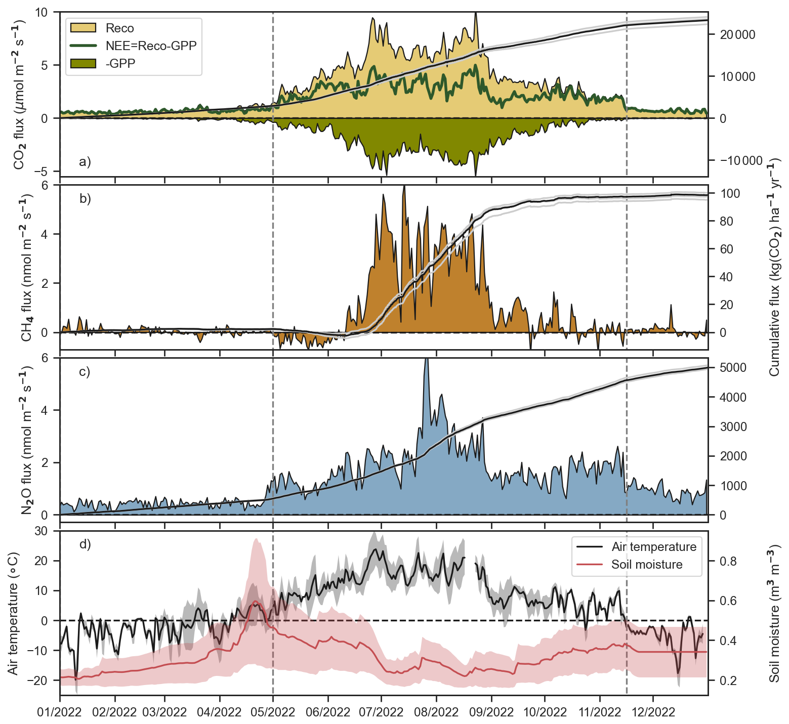
Figure 2 Time series of daily mean and cumulative sums of CO₂ (a), CH₄ (b) and N₂O (c) fluxes and daily air temperature and soil moisture (d) during the year 2022. The CO₂ flux is partitioned into the components of gross primary production (GPP) and ecosystem respiration (R_eco) using the methods described in Sect. 2.3. The vertical dashed lines indicate the snowmelt dates in spring and first snow in late autumn. Flux time series were gap-filled using three different ML algorithms (Sect. 2.3), and the cumulative sums calculated from these time series are shown using grey lines. The black line shows the ensemble average of these three estimates. The shaded area in panel (d) shows daily temperature and soil moisture variability (standard deviation) around the mean.

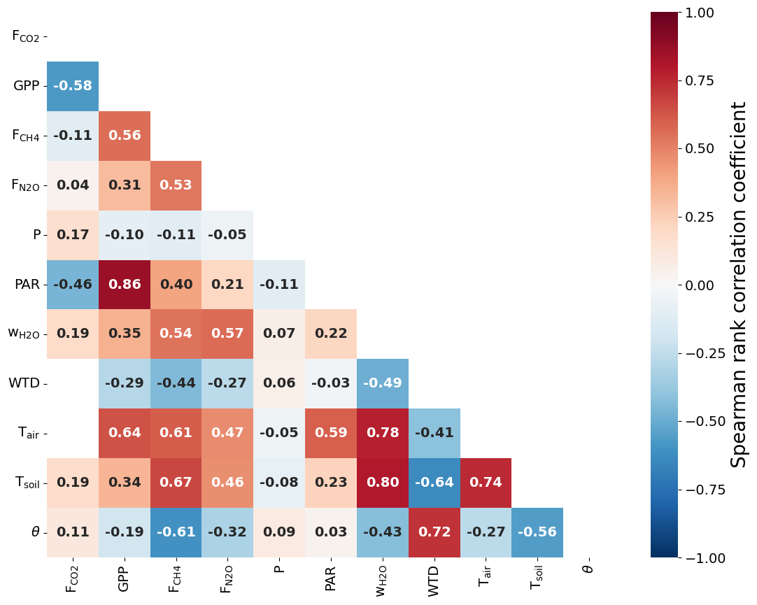
Figure 3 Correlation heatmap reporting Spearman's rank correlation coefficients for GHG fluxes and selected environmental parameters. The abbreviations used in the figure are as follows: $F_{{\mathrm{CO}}_{\mathrm{2}}}$ – CO₂ flux, GPP – gross primary productivity, $F_{{\mathrm{N}}_{\mathrm{2}}\mathrm{O}}$ – N₂O flux, $F_{{\mathrm{CH}}_{\mathrm{4}}}$ – CH₄ flux, P – precipitation, PAR – photosynthetically active radiation, $w_{{\mathrm{H}}_{\mathrm{2}}\mathrm{O}}$ – water mixing ratio in air, WTD – water table depth, T_air – air temperature, T_soil – soil temperature at 5 cm depth (averaged value obtained from three different sensors located over the CC area; see white circles in Fig. 1) and θ – soil water content at 5 cm depth (average value similar to T_soil). For further details on the measurement locations of other parameters, please refer to Fig. 1 and Sect. 2.2. Only correlations with a p value lower than 0.05 are shown.

3.2 Flux correlation with environmental parameters

Figure 3 shows correlation coefficients between the 30 min GHG fluxes and environmental variables. The NEE only correlated well ($\left|r_{\mathrm{s}}\right|\mathit{>}\mathrm{0.25}$) with PAR, whereas the GPP was correlated with PAR, $w_{{\mathrm{H}}_{\mathrm{2}}\mathrm{O}}$, and both T_air and T_soil. $F_{{\mathrm{CH}}_{\mathrm{4}}}$ was correlated with all environmental variables besides P. $F_{{\mathrm{CH}}_{\mathrm{4}}}$ was positively correlated with temperature, $w_{{\mathrm{H}}_{\mathrm{2}}\mathrm{O}}$ and PAR, whereas it was negatively correlated with the WTD (i.e. higher $F_{{\mathrm{CH}}_{\mathrm{4}}}$ values are observed when the WTD is close to the surface) and θ. The correlation of $F_{{\mathrm{N}}_{\mathrm{2}}\mathrm{O}}$ with environmental factors was similar to $F_{{\mathrm{CH}}_{\mathrm{4}}}$, except that it was more weakly correlated with PAR, WTD, θ, T_air and T_soil. Most of the environmental variables are correlated with each other due to their similar diel and annual cycles.

3.3 Models for CH₄ and N₂O fluxes to estimate surface-type-specific fluxes

The performance of each model is shown in Table S1. We selected the best models (based on) for further analysis: full θ ST9 for both $F_{{\mathrm{N}}_{\mathrm{2}}\mathrm{O}}$ and $F_{{\mathrm{CH}}_{\mathrm{4}}}$

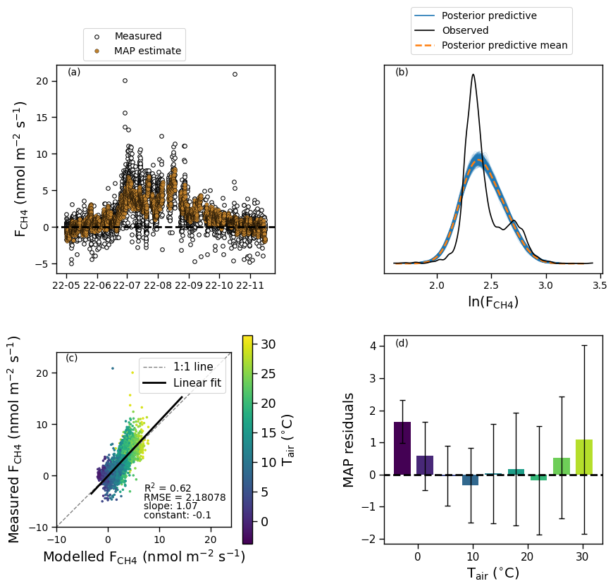
Figure 4 Time series of the measured and modelled CH₄ flux (a), the distribution of the measured CH₄ flux and the posterior predictive distributions (b), a scatter plot of the modelled versus measured CH₄ flux (c), and the model residuals as a function of air temperature (d). The model estimates are calculated using the maximum a posteriori (MAP) estimate of the parameters.

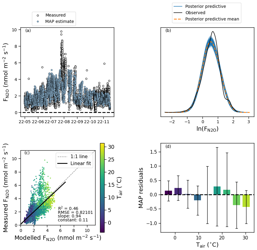
Figure 5 Time series of the measured and modelled N₂O flux (a), the distribution of the measured N₂O flux and the posterior predictive distributions (b), a scatter plot of the modelled versus measured N₂O flux (c), and the model residuals as a function of air temperature (d). The model estimates are calculated using the maximum a posteriori (MAP) estimate of the parameters.

For CH₄, the posterior predictive distribution (Fig. 4b) of the best model showed that the model both over- and underestimated the measurements, which were distributed very narrowly with two peaks at $\ln \left(F_{{\mathrm{CH}}_{\mathrm{4}}}\right)=\mathrm{2.35}$ (0.5 nmol m⁻² s⁻¹) and $\ln \left(F_{{\mathrm{CH}}_{\mathrm{4}}}\right)=\mathrm{2.75}$ (5.6 nmol m⁻² s⁻¹). The best model for CH₄ could capture 62 % of the variation in the measurements. The model parameters (Fig. 6a, b) indicate that the flux has weak temperature dependency except for ditches, high base source strength (α) and a low surface-type-specific base strength modifier (γ), except for plant-covered ditches. This suggests that there are no major differences in the source strengths between the surface types, except for the plant-covered ditches, from which the emissions are clearly higher than from other parts of the CC area.

The posterior predictive distribution for the best $F_{{\mathrm{N}}_{\mathrm{2}}\mathrm{O}}$ model shows a better fit to the observations (Fig. 5b) but fails to capture the peak N₂O emissions observed at the end of July (Fig. 5a). The R² value between the modelled and measured flux is 0.46, lower than for the best $F_{{\mathrm{CH}}_{\mathrm{4}}}$ model. The best $F_{{\mathrm{N}}_{\mathrm{2}}\mathrm{O}}$ model indicates higher variation between fluxes from different surface types than the model for $F_{{\mathrm{CH}}_{\mathrm{4}}}$ (Fig. 6c). Similarly, the temperature-dependency-defining parameter δ varies more between different surface types than it did for $F_{{\mathrm{CH}}_{\mathrm{4}}}$ (Fig. 6d). The model residuals (calculated with the MAP estimate) for both GHGs do not show a clear dependency on the air temperature (Figs. 4d, 5d), indicating no clear over- or underfitting with respect to a certain temperature range.

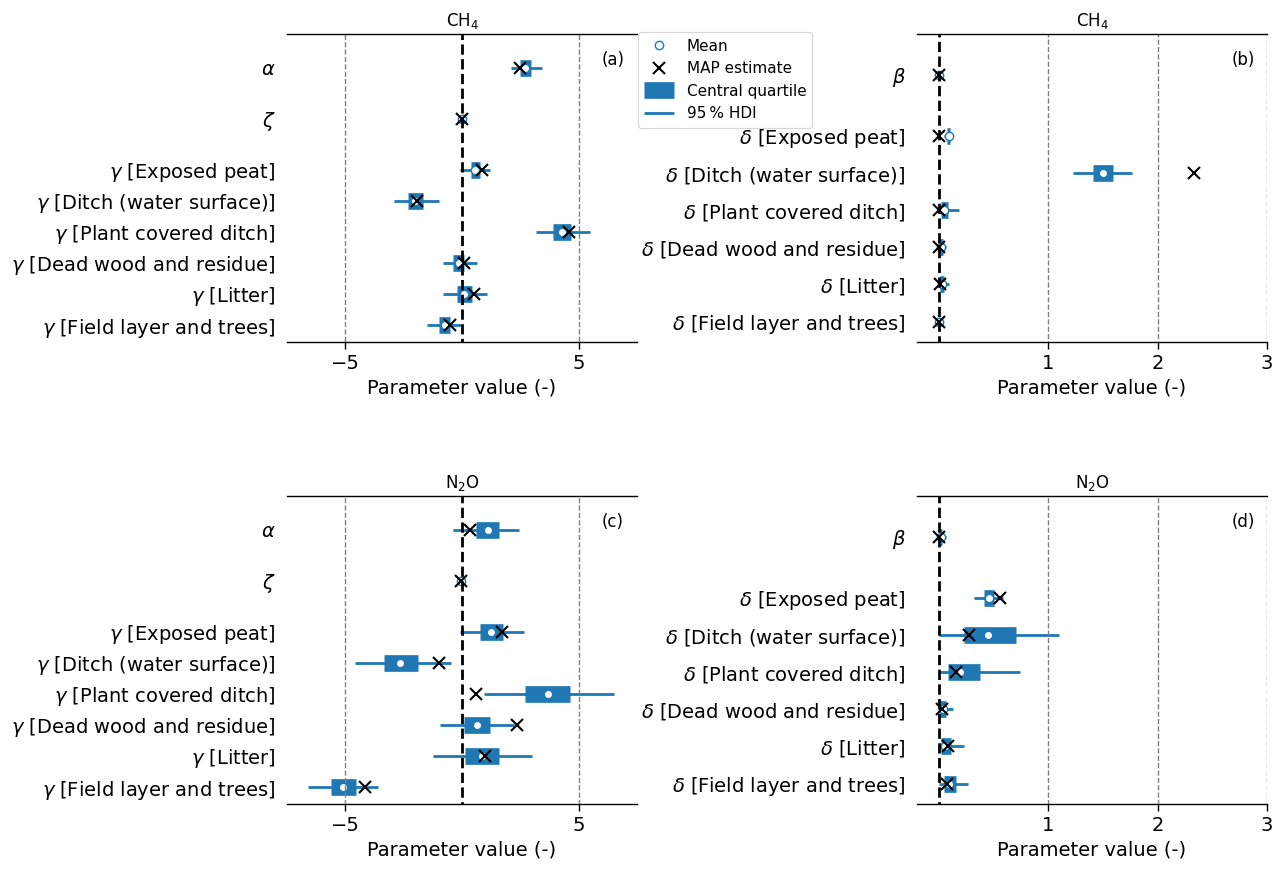
Figure 6 The 95 % highest posterior density interval for parameters of the best models for CH₄ (a, b) and N₂O (c, d). The bold line indicates the 25th and 75th percentiles of the distributions, white circles are the distribution means, and black crosses show the maximum a posteriori (MAP) estimate.

Figure 7 shows the distribution of the modelled surface-type-specific fluxes, predicted by setting the corresponding surface-type contribution to unity (${\mathit{\phi }}_{i,j}=\mathrm{1}$ for each j in Eq. 7) and calculating the 95 % highest density interval (HDI) of the resulting model using the measured T_air. The results are extrapolations of the underlying model to visualize the model parameters in Fig. 6.

The highest CH₄ emissions originate from plant-covered ditches (Figs. 6a, 7a), while emissions from the exposed peat and litter are over an order of magnitude smaller. The other surface types show low uptake and emissions of CH₄. Living trees and litter show the highest N₂O emissions (Figs. 6c–d, 7c–d). The second-highest N₂O emission come from dead wood and plant-covered ditches.

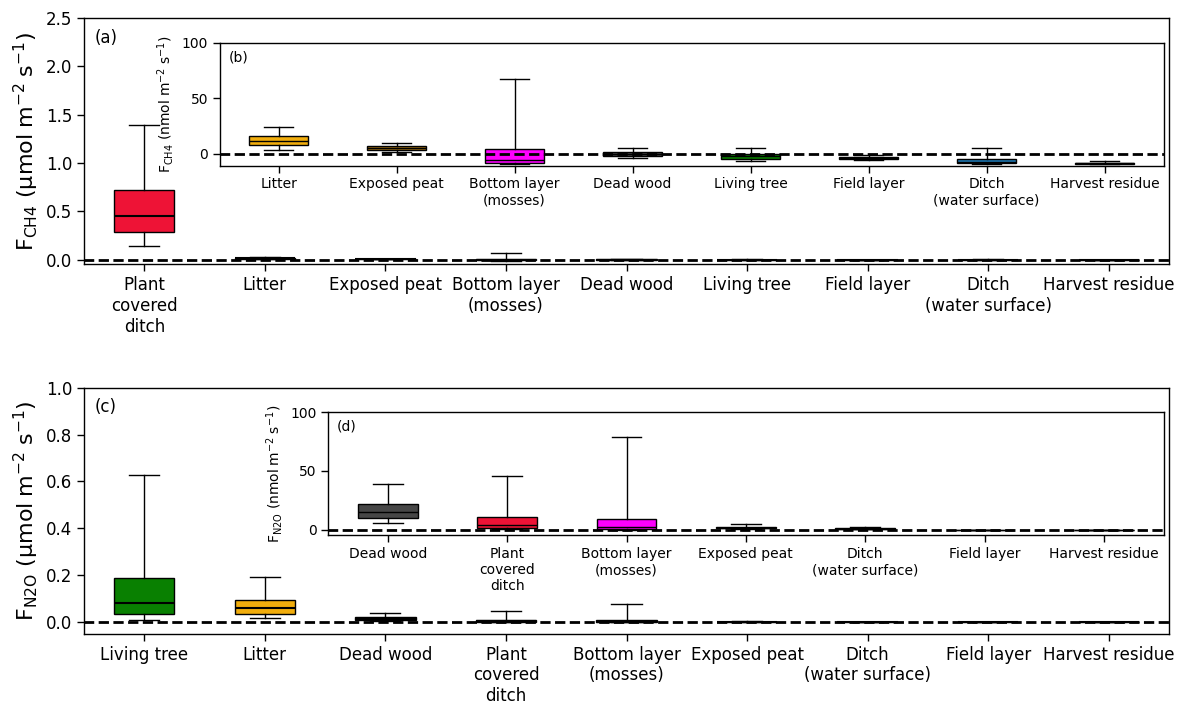
Figure 7 The surface-type-specific flux of CH₄ (a, b) and N₂O (c, d) fluxes. The surface-type-specific fluxes are calculated by setting the corresponding surface-type contribution to unity (${\mathit{\phi }}_{i,j}=\mathrm{1}$ for each j in Eq. 7) and calculating the 95 % highest density interval of the resulting model with the measured T_air. The box plot whiskers represent the 5th and 95th percentiles of the flux value distribution, the edges of the post represent the 25th and 75th percentiles, and the black horizontal line shows the median of the distribution. The box plots are ordered by the 75th percentile. Note the different scales of the y axis for each panel and that the fluxes are per square metre of the respective surface type. To estimate the contribution of each surface type to the total flux, values in this figure need to be multiplied by the fraction of the surface type in the clear-cut area or in the EC footprint presented in Table 1.

Figures S7 and S8 show how the modelled flux changes when surface types are added to the model one by one as well as how the model results agree with chosen measurements. From the analysis, it is evident that the most important surface types for the footprint-average CH₄ emissions are the plant-covered ditches (areal coverage of 1.1 %; Table 1) and exposed peat (29 %). For N₂O emissions, the most important surface types are exposed peat, litter (19.9 %), dead wood (22.8 %) and field layer (11.8 %).

Figures S9–S12 show the estimated parameters for the full θ models for the other numbers of STs. Interestingly, for CH₄, when the two types of ditches are lumped into one ST, their γ estimate is close to zero (Figs. S9, S11), whereas when the ditches are considered to be separate STs, the estimated γ for the plant-covered ditch class is the highest, while the γ for the ditch (water surface) class is the lowest, which is the same behaviour that we see in Fig. 6 for the best model.

The parameter estimates between different numbers of STs for N₂O models differ more those for CH₄ models. For example, for ST6 (Fig. S12), the highest γ MAP estimate is for dead wood and residue, whereas the γ for the field layer and trees is the smallest. The γ estimates for ST5 (Fig. S11) also seem to emphasize the role of litter, dead wood and residue as high-N₂O-emission surface types. It should be noted that living trees are always lumped together with some other surface type/types for all other numbers of STs. This might be the reason that the full θ no δ ST9 model clearly outperforms the full θ ST6 model for N₂O but not for CH₄ (Table S1).

Finally, we calculated the total emissions for CH₄ and N₂O for the snow-free period using the best full θ models and compared them to EC measurements (Table 3). The model estimates were calculated using the areal fraction of each surface type in the whole clear-cut (Table 1), instead of the areal fraction of the surfaces in the EC footprints. This way the reported modelled flux estimates are representative of the whole clear-cut area. The predicted cumulative CH₄ emission is 60 % smaller than that based on EC estimates, whereas the N₂O emissions from EC estimates are ca. 1.25 times higher than the median model prediction. This might be due to either model inaccuracies (see Figs. 4 and 5) or the EC footprint observing a biased sample of the ecosystem–atmosphere exchange (i.e. certain surface types have higher/lower areal coverage in EC footprints than they have in the whole clear-cut; see Table 1). However, the EC-derived emission estimate is inside the 95 % highest density interval for both GHGs.

Table 3 Comparison of methane and nitrous oxide emissions obtained from the EC measurements and predicted for the whole clear-cut area by the models that best described the temporal variability in fluxes. Note that the snow-free period is from 1 May to 16 November. For the modelling approach, the first value represents the median model prediction, while the values in parentheses present the 95 % highest density interval of the distribution of the snow-free period emissions calculated with the parameters estimated in the MCMC run. For the EC results, the values show the total emissions calculated from time series gap-filled with an ML ensemble, while the values in parentheses show the range of values calculated from time series gap-filled using different ML algorithms (see Sect. 2.3). Note that the shares of each surface type in the whole clear-cut were used to calculate the modelled flux estimates; hence, they relate to the whole clear-cut area, not to the EC footprint area.

4 Discussion

4.1 Impact of surface types on CH₄ and N₂O fluxes

We built a statistical model to separate observed CH₄ and N₂O fluxes into their surface-type and environmental controls using the flux time series and surface-type composition for each measurement period inferred from drone-based surface characterization and an analytical footprint model. The aims of the analysis were to assess whether the fluxes vary across different surface types and to detect the key surface types contributing to the net emissions. The models suggest that plant-covered ditches and exposed peat are the most important surface types for CH₄ emissions (Figs. 6, 7, S7), whereas other surface types contributed much less or acted as CH₄ sinks. This is consistent with chamber measurement at this study site, which showed that soils acted as CH₄ sinks, as the aerobic soil layer above the water table is able to consume CH₄ from both the deep soil and the atmosphere. The high CH₄ emissions observed in ditches can be attributed to two main factors: the high production of CH₄ in anaerobic ditch sediments and the transport of CH₄ from surrounding soils by drainage water. Rissanen et al. (2023) found that ditches with open water exhibited higher emissions than those covered by plants. In particular, ditches covered by mosses showed very low emissions, as CH₄ can be oxidized in the moss layer. Minkkinen and Laine (2006) reported that the CH₄ emissions from ditches varied considerably depending on the water movement and vegetation cover. They found that ditches with moving water showed higher emissions, likely due to the transport of CH₄ from the surrounding areas. However, we found that the plant-covered ditch surface was the highest emission source, likely because the main ditch in close proximity to the EC tower was classified as plant-covered due to the vascular plants growing on the ditch bank (Fig. S1). It contributed the majority of the CH₄ emissions according to our analysis. It should be noted that our classification did not distinguish between moss- and vascular-plant-covered ditches. In contrast to mosses, which can act as a filter for CH₄ due to oxidation (Kolton et al., 2022; Larmola et al., 2010), some vascular plants, such as Eriophorum, can enhance the transport of CH₄ to the atmosphere (Minkkinen and Laine, 2006). The second-largest contributor to CH₄ emissions in our model was exposed peat. Pearson et al. (2012) observed that the contrasting effects of mounding with exposed peat on CH₄ emissions from soil depends on the drainage conditions. Soil CH₄ emissions depend on production, consumption and transport processes. Production is largely controlled by the WTD, which determines the anoxic layer, whereas the surface types in clear-cut with distinct topography and ground vegetation can affect the consumption and transportation.

Measured N₂O fluxes showed strong temporal variation over the studied year (Fig. 2). The short periods of high N₂O emissions observed during the snow-free period, which contribute considerably to the annual budget, have been previously documented in peatland sites through continuous measurements based on EC and automatic chambers (Pihlatie et al., 2010). Our model was, however, unable to predict the high-N₂O-emission period observed during late July and early August. The high emissions are likely driven by the activity of specific archaea and prevailing conditions, including the temperature, moisture, $\mathrm{C}/\mathrm{N}$ ratio, nitrate content, pH and peat decomposition phase (Bahram et al., 2022). Our modelling approach, unfortunately, lacked some of these details. Furthermore, our study demonstrated that N₂O emissions during the snow-covered period constituted a significant (20 %) contribution to the annual budget. The winter under study was meteorologically typical, which may explain why the importance of these emissions is consistent with that reported in previous works (Rautakoski et al., 2024; Kim and Tanaka, 2002). However, the frequency of warm winters with lower snow cover and more freeze–thaw events is predicted to increase in northern latitudes (Ruosteenoja and Räisänen, 2021). As a result, N₂O emissions under snow-covered conditions are expected to increase in boreal forests. In terms of spatial variability, our model showed that the majority of N₂O emissions were attributable to surfaces with living trees, exposed peat, dead wood and litter (Figs. 6, 7, S8). A previous study, which employed chamber measurements, corroborates our modelling findings (Mäkiranta et al., 2012). It was observed that soils in peatland forests covered by logging residue exhibited high N₂O emissions after harvest, which was attributed to the decay of the logging residuals. Pearson et al. (2012) also found high N₂O emissions from the mounds (surfaces with exposed peat) following site preparation in a nutrient-poor clear-cut peatland forest. N₂O emissions were found to be highly dependent on the availability of N in the soil (Ojanen et al., 2010). Therefore, it can be concluded that the observed variation in N₂O emissions from different surface types may also be related to the spatial variability in the nutrient conditions within the studied clear-cut area.

Studies of soil microclimate and gas fluxes after clear-cutting and site preparation are scarce in drained peatland forests, but the few done using the manual chamber method (Pumpanen et al., 2004; Mjöfors et al., 2015; Strömgren et al., 2016, 2017) have shown that the spatial variability is typically very high. Pearson et al. (2012) applied the manual chamber method to assess the impact of varying microtopography following site preparation in a nutrient-poor clear-cut peatland forest for CO₂, CH₄ and N₂O. Gas fluxes from ditches can be measured using a manual chamber floating on ditch water (e.g. Minkkinen and Laine, 2006; Rissanen et al., 2023). However, ditch banks, where the ditch materials are exposed and may act as CH₄ hotspots, have rarely been measured due to the difficulty involved with installing chambers on uneven surfaces. Our surface-type model could facilitate the understanding of the contribution of surfaces to CH₄ and N₂O emissions, particularly those that have previously not been quantified or have been challenging to quantify. Furthermore, we identified the surface types that are likely to have high CH₄ and N₂O emissions after clear-cutting. These surface types should be targeted in future chamber studies to accurately quantify the surface-specific emission fluxes (or emission factors).

4.2 Methodological issues and outlook

The models for $F_{{\mathrm{CH}}_{\mathrm{4}}}$ and $F_{{\mathrm{N}}_{\mathrm{2}}\mathrm{O}}$ were found to explain slightly less than 62 % and 46 % of the observed temporal variation, respectively. Moreover, the model that best explained the variability in $F_{{\mathrm{CH}}_{\mathrm{4}}}$ produced a lower cumulative flux over the snow-free season for the whole clear-cut than what was measured by the EC from its footprint (Table 3). This disagreement might be either due to model inaccuracy or the slightly unrepresentative location of the EC tower (Table 1; see also Chu et al., 2021). However, the estimates were still within the 95 % HDI. The underlying assumptions in our model approach are (i) surface type variability drives the variability in soil processes underlying the fluxes, an assumption that can be tested using methods such as chamber studies; (ii) the relative contribution of surface types for each 30 min EC flux can be determined by footprint analysis; and (iii) the surface types can be reliably characterized from aerial RGB and multispectral images.

For both CH₄ and N₂O, we found a clear improvement in model predictions when the effect of surface types was introduced in the models (Table S1). For CH₄, the deviation in model performance between different surface-type-specific models was minor, suggesting that the CH₄ emissions may be less dependent on the surface type than N₂O emissions. The Bayesian inference method was selected for its capacity to incorporate prior knowledge into the model. With the Bayesian framework, we were able to define the surface-type-specific flux strength modifiers (γ_j parameters) in a hierarchical manner. This resulted in each surface type having a distinct base production distribution, while the mean of each distribution was derived from a common underlying distribution. Furthermore, there are other types of prior knowledge that could be incorporated into the model to improve the surface-type-specific flux estimates. For instance, chamber measurements of the surface-type-specific flux could be employed to inform the model development, particularly as they could be used as prior information to constrain the model (Ludwig et al., 2024). Results also revealed that there is a strong negative correlation between CH₄ and N₂O flux with soil water availability (Fig. 3), a finding that is consistent with previous observations in drained peatland forests (Ojanen et al., 2010). Inclusion of a soil-moisture-dependent term in the model improved the model's predictive performance. However, only a general soil moisture term was included. As moisture and microtopography vary across the clear-cut, distributed measurements of the water table (or soil moisture) would be necessary for further refinement of the model. We tested replacing the soil moisture with the WTD, but the models with the WTD performed worse than the full θ ST9 models for both compounds. Given that we only considered WTD measurement at one location, we cannot be sure that the soil moisture would outperform the WTD as an independent variable if we carried out more distributed measurements. Furthermore, the spatial variability in N₂O emissions might be further explained by variables describing nutrient availability (e.g. the $\mathrm{C}/\mathrm{N}$ ratio).

A few previous studies have used surface-type information and EC measurements to elucidate surface-type-specific fluxes. In a tundra ecosystem, Tuovinen et al. (2019) and Ludwig et al. (2024) developed a model for CH₄ flux by decomposing the total flux into the sum of fluxes from different surface types. In both studies, the models captured more distinct surface-type fluxes than our model for CH₄. Similarly, in peatlands, Franz et al. (2016) and Forbrich et al. (2011) were able to achieve a better agreement and more distinct surface-specific emissions with CH₄ modelled from surface-type-specific fluxes and EC measurements, compared with our CH₄ model. Moreover, Mazzola et al. (2021) found, based on chamber measurements, that there was a clear difference between surface-type-specific CH₄ emissions at a restored bog site in northern Scotland. One possible explanation for this discrepancy is that the surface types in our model are rather homogeneously distributed across our drained peatland clear-cut compared with the other sites, which makes the attribution of fluxes to different surface types more challenging, as their relative contribution within the flux footprint does not strongly depend on wind direction. Another possibility is that the proportion of some of the surface types inside the footprint is always so low that their contribution to the model estimate is diluted by the surrounding landscape (e.g. ditches with water surface). As a result, the model might not correctly capture their contribution to the flux. Regarding the N₂O emissions, we are not aware of any previous studies that have attempted to model surface-type-specific fluxes based on EC data. However, given that N₂O was the second-largest GHG source from the clear-cut area, it is evident that such studies are required in order to improve GHG budget estimation in the future.

For the best models, we also tested replacing T_air with mean soil temperature measured at the three locations shown in Fig. 1. For N₂O, this produced a slightly better fit in terms of ELPD-LOO (difference of 74 units). This suggests that, especially for understanding N₂O emissions, measuring the surface-type-specific soil temperature would be beneficial.

Footprint calculations were sensitive to the input parameters used in the calculations which, therefore, altered the estimation of surface-type-specific CH₄ and N₂O fluxes. For instance, the displacement height (d) was empirically estimated from data (see Sect. 2.3), and changing the estimation procedure altered the footprint results. This was because changes in d directly affected the effective measurement height (z−d), which is one of the main factors influencing the footprint size (e.g. Rannik et al., 2012). These uncertainties essentially stem from the fact that the clear-cut surface is heterogeneous, with varying plant heights and small-scale topography. The spatial heterogeneity varies with wind direction, and this altered the flow field observed with the EC equipment. Therefore, the estimation of descriptive values for all of the parameters needed by the footprint model, e.g. d, is uncertain.

Furthermore, it is important to note that simple footprint models, such as the Kljun model used in this study, are only strictly valid above the roughness sublayer, where individual surface roughness elements (e.g. trees and branch piles) no longer locally alter the flow. Even above the roughness sublayer, they rely on simplified theories on the flow field, such as the Monin–Obukhov theory, which are unable to handle complications such as non-stationarities. Nevertheless, such models are also utilized in complex roughness sublayer flows (Chu et al., 2021) to link the observed turbulent fluxes to surface features (Stagakis et al., 2019). It is likely that our EC tower was frequently within the roughness sublayer. Although simple footprint models have been shown to produce reasonable estimates of flux source areas in ideal measurement locations (Arriga et al., 2017; Heidbach et al., 2017; Nicolini et al., 2017; Dumortier et al., 2019; Rey-Sanchez et al., 2022), it is unclear how the estimates are affected by the roughness sublayer flow. The presence of surface roughness elements increases turbulent mixing, which may result in shorter footprints than would be expected for flows above smoother surfaces. Nevertheless, the empirically estimated values for d and z₀ may already partly account for this. The methodology used here to derive surface-type-specific fluxes did not consider the aforementioned uncertainties. Furthermore, in the Bayesian framework, we assumed that the footprints were observed perfectly. This simplification should be kept in mind when analysing the surface-type-specific fluxes.

Our results suggest that the emissions from multiple surface types (Figs. 6, 7) are very similar and that some surface types contribute little to the footprint-average fluxes (Figs. S7, S8). This implies that a more detailed surface-type characterization would have improved the model performance. The methods used for surface characterization hold promise for following clear-cut vegetation dynamics to address the vegetation recovery after site preparation and planting. More detailed vegetation classification was examined, but this was found to be difficult, as the vegetation after clear-cutting was sparse and plant sizes were small. This caused the number of polygons for some vegetation classes in the training data to be very low. The vegetation growing in ditches had a larger and more uniform surface area, and the classification of that vegetation would be easier than that of individual saplings. The topography of the studied site is flat, which makes the classification between the ditch, tree and other vegetation types using the drone-derived elevation model more accurate. Here, we could utilize precise georeferencing, using ground control points accurately measured in the open area of the site. For more detailed vegetation surveys, the resolution of the drone orthomosaic could still be increased to determine the leaf and branch structure of the smallest plants, as the spectral differences are not only defined by species but also by factors such as plant health (Grybas and Congalton, 2021; Zhou et al., 2021). Parameters describing the structure, such as the grey-level co-occurrence matrix, should also be used for classification. Alternatively, deep learning methods provide high classification accuracy by taking the structure into account without parameterization (Onishi and Ise, 2021). Using the same sensors, increased resolution could be achieved by lowering the flight altitude, resulting in an increased flight time and battery capacity requirement. In addition, increased resolution can make generating training data and validating results more difficult as the number of segments increases and it is more difficult to decide which class the polygon represents, especially at sites like clear-cut areas with very detailed surface cover requiring multiple surface-type classes.

4.3 Clear-cut peatland forests are net GHG sources

Despite the importance of peatland forests in Nordic countries, little is known about the impacts of harvesting practices and alternative management chains on their GHG balance dynamics. In particular, GHG fluxes occurring shortly after clear-cutting and stand establishment have been rarely quantified (Mäkiranta et al., 2010; Korkiakoski et al., 2019, 2023). In this study, we employed the EC technique to quantify the CO₂, CH₄ and N₂O fluxes from a recent clear-cut area that had been regenerated by planting after site preparation and ditch network maintenance. The findings demonstrate that our previously spruce-dominated fertile peatland forest was a major source of GHG emissions during the first full year (second growing season) after clear-cutting and site preparation. The results indicate that CO₂ is the primary contributor to the annual GHG balance, accounting for 83 % (23.3 t CO_2 eq. ha⁻¹ yr⁻¹) of the total global warming potential of the GHG emissions. It is also important to note that the CO₂ source strength of the clear-cut area was ca. 10 t CO_2 eq. ha⁻¹ yr⁻¹ larger than the NEE before clear-cutting (13.2 t CO_2 eq. ha⁻¹ yr⁻¹; Laurila et al., 2021). Our results are consistent with those of previous studies on forested peatlands. A relatively similar fertile drained mixed-forest peatland (Lettosuo) in southern Finland was found to be CO₂-neutral before harvesting, as observed by EC measurements (Korkiakoski et al., 2023). After clear-cutting and site preparation, the ecosystem turned into a strong CO₂ source, initially emitting 31 t CO_2 eq. ha⁻¹ yr⁻¹, although emissions decreased to 8.2 t CO_2 eq. ha⁻¹ yr⁻¹ a total of 6 years after harvest. This decrease was attributed to the increased CO₂ uptake by emerging vegetation and the concomitant decrease in CO₂ release from decomposing cutting residue (Korkiakoski et al., 2023). At our site, the recovery of ground vegetation was observed to be significant with respect to GPP (14.9 t CO_2 eq. ha⁻¹ yr⁻¹) as soon as the second post-harvest growing season. This partially offset more than 35 % of R_eco, which was mostly associated with CO₂ emissions. In a more southern minerotrophic drained forested peatland (Tobo) in the Uppsala region of Sweden, CO₂ emissions were quantified using chamber-based methods, with values ranging from 27 to 50 t CO_2 eq. ha⁻¹ yr⁻¹ in the second year following clear-cutting, depending on ditch management (Tong et al., 2022). Furthermore, Mäkiranta et al. (2010) reported that chamber-based estimates of CO₂ emissions during the growing season from a clear-cut drained oligotrophic peatland (Vesijako) located in southern Finland varied between 16 and 23 t CO_2 eq. ha⁻¹ during the first 3 years after clear-cutting.

The net CO₂ emissions from our study site (Ränskälänkorpi clear-cut area) are comparable to EC-based measurements by Ahmed (2019) (20 t CO_2 eq. ha⁻¹ yr⁻¹) after clear-cutting of a fertile Norway spruce stand on mineral soil in Hyytiälä, southern Finland. Furthermore, our values are 20 % –30 % larger than the CO₂ emissions from 1- to 3-year-old clear-cuts on mineral soils in southern and central Sweden (16–18 t CO_2 eq. ha⁻¹ yr⁻¹) (Grelle et al., 2023). Kolari et al. (2004) observed smaller emissions (14 t CO_2 eq. ha⁻¹ yr⁻¹) 4 years after clear-cutting an infertile Scots pine stand on mineral soil in southern Finland. At Norunda, Sweden, a clear-cut former Norway spruce forest on mineral soil with a shallow water table was identified as net source of CO₂ (NEE; 16 t CO_2 eq. ha⁻¹ yr⁻¹) during the first and second year after harvest (16 and 11 t CO_2 eq. ha⁻¹ yr⁻¹, respectively). At this site, GPP and R_eco exhibited fluctuations ranging between 5–14 and 21–23 t CO_2 eq. ha⁻¹ yr⁻¹, respectively (Vestin et al., 2020).

The contribution of N₂O and CH₄ emissions to the total annual GHG balance remained small, despite their much higher global warming potential. Specifically, the contribution of N₂O emissions was 17.6 % (5.0 t CO_2 eq. ha⁻¹ yr⁻¹), while CH₄ had only marginal importance (0.1 t CO_2 eq. ha⁻¹ yr⁻¹; 0.4 %). The negligible share of CH₄ to net GHG emissions is in line the findings at the Lettosuo and Tobo sites (Korkiakoski et al., 2019; Tong et al., 2022). Korkiakoski et al. (2019) estimated, from chamber measurements, that N₂O emissions from the Lettosuo site were 3.7 g N₂O m⁻² yr⁻¹ after clear-cutting, resulting in more than 11 t CO_2 eq. ha⁻¹ yr⁻¹. According to Tong et al. (2022), N₂O emissions after clear-cutting at the Tobo site contributed only 0.53 %–1.3 % to the total GHG emissions, likely due to (1) the fact that the biweekly chamber sampling may have missed some of the high emission peaks and (2) the low soil moisture, as the water table depth was low compared with similar studies. Note that prior studies have utilized temporally and spatially discontinuous chamber measurements for observing N₂O and CH₄ fluxes. Vestin et al. (2020) observed net CH₄ emissions of between 0.3 and 1.5 t CO_2 eq. ha⁻¹ yr⁻¹ and N₂O emissions of between 0.8 and 1.1 t CO_2 eq. ha⁻¹ yr⁻¹ from the Norunda clear-cut using the flux-gradient approach. To the best of our knowledge, this study is the first to document EC-based N₂O and CH₄ fluxes from a forest ecosystem after clear-cutting.

Our results confirm earlier findings (e.g. Korkiakoski et al., 2023) that clear-cutting increases the GHG emissions from forested boreal peatlands, at least in the short term, when compared with mature forests (Minkkinen et al., 2001; Ojanen et al., 2010; Alm et al., 2023). To evaluate the climate effects of alternative harvesting methods (e.g. continuous cover forestry) compared with rotation forestry and clear-cutting, the post-harvest dynamics of GHG emissions must be better known, which necessitates more and longer follow-up studies (Korkiakoski et al., 2023). In Finland, 390 000 ha of fertile drained peatlands will soon be subject to a choice (with respect to their management) between (1) clear-cutting and second even-aged rotation or (2) conversion to other management regimes, such as continuous cover forestry (Lehtonen et al., 2023) or partial rewetting. It is currently estimated that the conversion to continuous cover forestry (which excludes clear-cutting but permits frequent heavy thinnings from above) could result in an annual reduction in the clear-cut area in fertile peatlands of 16 000 ha yr⁻¹ (Lehtonen et al., 2023). It is therefore evident that comparative long-term studies (as well as modelling) between rotation forestry with clear-cutting and alternative harvesting approaches across a spectrum of site characteristics are needed to facilitate the development of effective harvest management strategies to mitigate GHG emissions, especially those of CO₂ from peat decomposition, in forested boreal peatlands.

5 Conclusions

We measured CO₂, CH₄ and N₂O fluxes in the second growing season after the clear-cutting of a Norway-spruce-dominated drained boreal peatland forest in southern Finland using eddy-covariance-based measurements. In the second growing season, the clear-cut area was a significant source of GHG emissions, with the annual total GHG balance dominated by CO₂ emissions (23.3 t CO_2 eq. ha⁻¹ yr⁻¹ or 22.4–24.1 t CO_2 eq. ha⁻¹ yr⁻¹, depending on the EC gap-filling method; 82.0 % of the total). The N₂O emissions (5.0 t CO_2 eq. ha⁻¹ yr⁻¹ or 4.9–5.1 t CO_2 eq. ha⁻¹ yr⁻¹) contributed 17.6 %, while the role of CH₄ flux (0.1 t CO_2 eq. ha⁻¹ yr⁻¹ or 0.1–0.1 t CO_2 eq. ha⁻¹ yr⁻¹; 0.4 %) was negligible. We note that our study represents only a partial overview of a rapidly evolving forest ecosystem and that longer studies are needed to better understand the GHG budget of clear-cut boreal peatland forests. However, the results presented herein reinforce the recently established understanding that clear-cut peatland forests are a significant source of GHGs.

Using the drone-based surface classification, EC measurements and statistical modelling, we estimated surface-type-specific CH₄ and N₂O fluxes. The best-fitting models revealed that the highest CH₄ emissions in the study area originated from the plant-covered ditches and exposed peat, while the highest N₂O emissions occurred from the exposed peat, litter, dead wood and living trees.

The role of exposed peat as a CH₄ and N₂O emitter suggests the need for more detailed studies to understand the processes within this surface type. Based on this study, reducing the amount of exposed peat after clear-cutting would be beneficial with respect to decreasing the CH₄ and N₂O emissions to the atmosphere. Similarly, reducing the litter input to the ground during harvesting would be beneficial with respect to decreasing N₂O emissions. The plant-covered ditches are important for the CH₄ emissions based on the modelling; therefore, how the CH₄ emissions change with respect to different plant species poses an interesting future question.

Finally, we note that our results are based on statistical modelling; thus it is recommend that manual chamber-based measurements be conducted in parallel with EC-based measurements to better constrain and validate surface-type-specific flux estimates for better forest management of drained forested boreal peatlands.