Temporal dynamics and environmental controls of carbon dioxide and methane fluxes measured by the eddy covariance method over a boreal river

Boreal rivers and streams are significant sources of carbon dioxide (CO₂) and methane (CH₄) for the atmosphere. Yet the controls and the magnitude of these emissions remain highly uncertain, as current estimates are mostly based on indirect and discrete flux measurements. In this study, we present and analyse the longest CO₂ and the first ever CH₄ flux dataset measured by the eddy covariance (EC) technique over a river. The field campaign (Kitinen Experiment, KITEX) was carried out during June–October 2018 over the river Kitinen, a large regulated river with a mean annual discharge of 103 m³ s⁻¹ located in northern Finland. The EC system was installed on a floating platform, where the river was 180 m wide and with a maximum depth of 7 m. The river was on average a source of CO₂ and CH₄ for the atmosphere. The mean CO₂ flux was 0.36 ± 0.31 µmol m⁻² s⁻¹, and the highest monthly flux occurred in July. The mean CH₄ flux was 3.8 ± 4.1 nmol m⁻² s⁻¹, and it was also highest in July. During midday hours in June, the river acted occasionally as a net CO₂ sink. In June–August, the nocturnal CO₂ flux was higher than the daytime flux. The CH₄ flux did not show any statistically significant diurnal variation. Results from a multiple regression analysis show that the patterns of daily and weekly mean fluxes of CO₂ are largely explained by partial pressure of CO₂ in water ($p{{\mathrm{CO}}_{\mathrm{2}}}_{\text{w}}$), photosynthetically active radiation (PAR), water flow velocity and wind speed. Water surface temperature and wind speed were found to be the main drivers of CH₄ fluxes.

1 Introduction

The global river network covers an area of about 624 000 km², which is approximately 15 % of the global inland water area (Raymond et al., 2013; Verpoorter et al., 2014). Despite their relatively small area, rivers and streams are significant sources of carbon (C) for the atmosphere in the form of carbon dioxide (CO₂) and methane (CH₄) (Raymond et al., 2013). Prior studies have estimated that 0.23–1.8 Pg C yr⁻¹ is released to the atmosphere from streams and rivers, mainly in the form of CO₂ (Cole et al., 2007; Aufdenkampe et al., 2011; Raymond et al., 2013; Regnier et al., 2013; Lauerwald et al., 2015; Drake et al., 2018). As methane is a more potent greenhouse gas than carbon dioxide, its emission from rivers is of importance, although the CH₄-C only accounts for a few percent of the total carbon flux (Cole et al., 2007). The most recent estimate of the outgassing magnitude for CO₂ was published by Li et al. (2021), who combined studies from 595 streams and rivers. Their global estimate for CO₂ annual emission is 1.8 Pg C of which 72.3 % takes place in streams (Strahler orders 1–3) (Li et al., 2021). For CH₄, the most recent outgassing estimate is 27.9 Tg CH₄ per year (Rocher-Ros et al., 2023).

By far, most of the river gas flux studies so far have been conducted using floating chambers that are point measurements in time and space (Bastviken et al., 2015; Lorke et al., 2015). In addition, the flux measurements and gas sampling tend to concentrate on daytime hours (Gómez-Gener et al., 2021) and mostly during calm and moderate wind speeds with good weather conditions. Due to the magnitude of surface-layer turbulence and the processes producing or consuming CO₂ or CH₄ being dependent on location and time (Rocher-Ros et al., 2019; Gómez-Gener et al., 2021; Attermeyer et al., 2021), there is inherently large spatial and temporal variability in the flux magnitude, which may not be captured with floating chambers (Hall and Ulseth, 2019). The eddy covariance (EC) method, which provides flux estimates for a certain averaging period and represents a much larger spatial domain than chambers, has been utilised over a river – so far only once for CO₂ flux (Huotari et al., 2013) and never for CH₄. Therefore, due to the lack of continuous and long-term flux time series, knowledge gaps exist in resolving the diurnal, seasonal and interannual variability of the air–water gas exchange and in the significance of different physical and biogeochemical processes in rivers and streams of different sizes.

To address this gap, we conducted an experiment on the subarctic river Kitinen in northern Finland during June–October 2018 for the Kitinen Experiment (KITEX) campaign. The goal of the campaign was to measure and quantify the CO₂ and CH₄ fluxes ($F_{{\mathrm{CO}}_{\mathrm{2}}}$ and $F_{{\mathrm{CH}}_{\mathrm{4}}}$, respectively) with an EC system on a floating platform as well as the physical forcings driving the fluxes. The aims of this study are to provide 4-month time series of both CO₂ and CH₄ fluxes and to quantify the response of the fluxes to different environmental drivers. In addition, we present the diurnal patterns of the gas fluxes, analyse their possible causes, and discuss to what extent the under-representation of flux temporal dynamics in existing databases, largely based on discrete sampling, may bias estimates of CO₂ and CH₄ emissions from river systems. Finally, we propose a new approach to attempt to minimise the effect of a limited fetch on the measured fluxes, providing more information on the use of the EC technique in relatively small inland water bodies.

2 Material and methods

2.1 Site description

The river Kitinen in northern Finland is 235 km long and has a catchment area of 7672 km² (Fig. 1a). The catchment area mostly consists of managed boreal forest with Scots pine (Pinus sylvestris) and Norway spruce (Picea abies) as the main tree species, wetlands of which a large portion is drained, small streams and rivers, some low mountains, and a few small settlements. Forests cover approximately 67 % and wetlands 25 % of the catchment. The soil in the catchment area mainly consists of sandy moraine and peat. The catchment area is relatively flat, with the height above sea level being 100–200 m in the south and 200–300 m in the north and exceeding 400 m only in a few places. Consequently, the mean slope of the river is just 0.5 m km⁻¹. The river Kitinen is heavily regulated with, altogether, seven hydropower plants and corresponding reservoirs along its length. The river is a tributary of the larger Kemijoki.

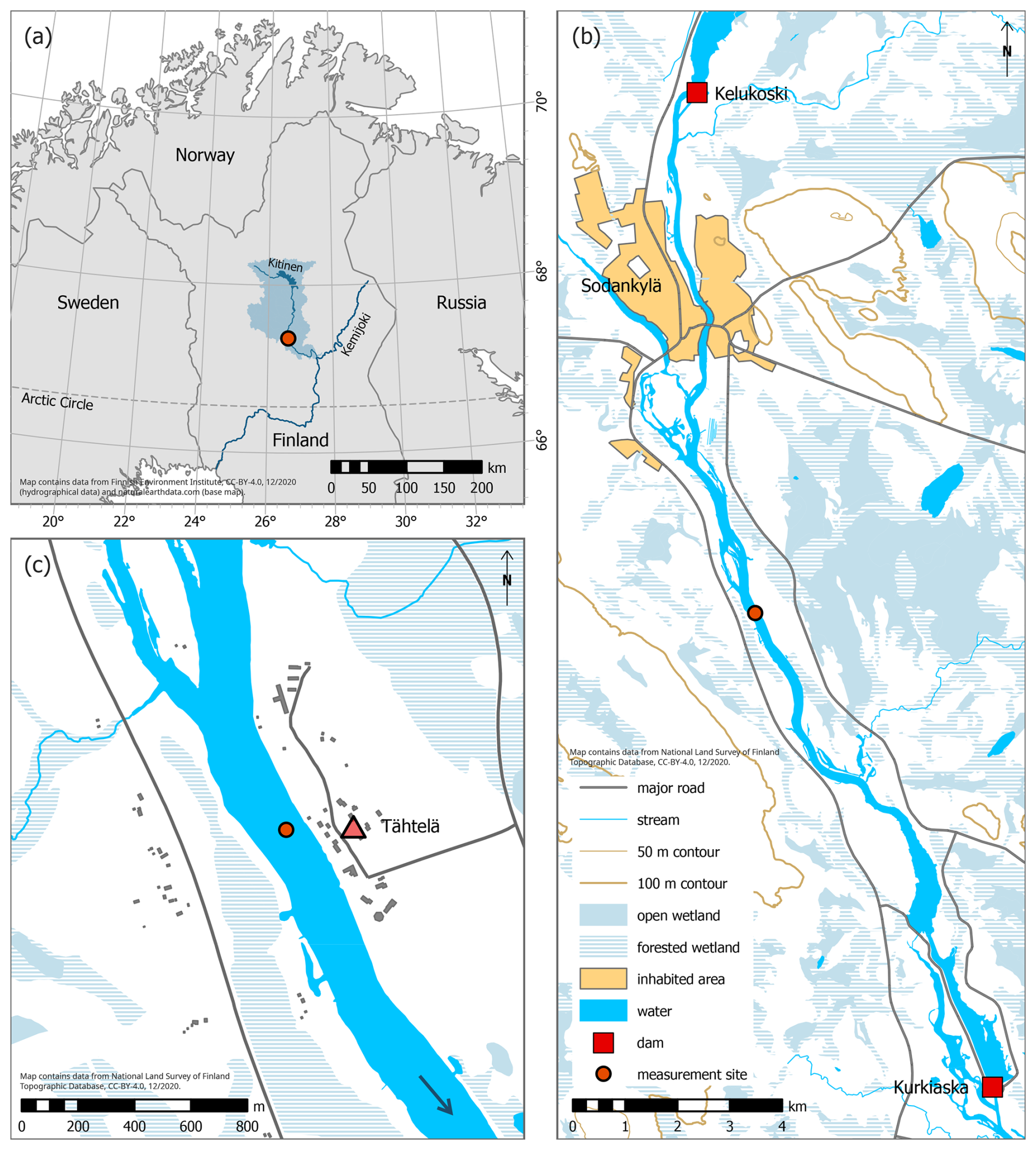
Figure 1 (a) Location of the river Kitinen (blue line) and its catchment area (light-blue area) in northern Finland. The site of the experiment is marked with a red dot. The larger Kemijoki is drawn with a dark blue line. (b) General area of the measurement site. Hydropower plants closest to the site are indicated with red squares. (c) Immediate surroundings of the experiment site. The arrow indicates the flow direction. The red triangle shows the location of the Tähtelä weather station. Buildings are marked with grey polygons.

Kitinen's catchment area belongs to the subarctic climate zone (Köppen classification Dfc). The annual mean temperature (related to the Finnish Meteorological Institute's reference period 1991–2020) is 0.3 °C, and the annual mean precipitation is 543 mm. Permafrost does not exist in the region. The vegetation-growing period in the area normally lasts from mid-May until late September. The river freezes every winter, usually in October–November, and the ice breakup normally takes place in May. In 2018, the breakup occurred in mid-May.

The experiment site (67.37 °N, 26.62 °E; 173 m above sea level) was located next to the Finnish Meteorological Institute's research and weather station in Tähtelä (Fig. 1b–c), 5 km south of the town of Sodankylä. At the experiment location, the river is 180 m wide and forms a straight section extending approximately 600 m upstream and 1000 m downstream from the site. The direction of the river at the site is roughly north-northwest–south-southeast, and it flows towards the south. The mean annual discharge, measured at the closest power plant downstream, is 103 m³ s⁻¹. The maximum depth at the site is 7 m. The river bed consists mainly of sand with some overlaying biological deposits. The river Kitinen's Strahler stream order at the site is 5, based on hydrographical data that include headwater streams with a catchment area larger than 10 km².

The closest hydropower plants to the site are located 11 km upstream and 11 km downstream. The water flow velocity at the experiment site was almost completely controlled by the hydropower dam regulation downstream. Flow regulation in the river followed a certain pattern where the flow would be low or completely halted during most nights (Guseva et al., 2021).

The eddy covariance, meteorological and water flow measurements were conducted on a floating platform, located about 70 m from the eastern river bank, where the water depth was 4.5 m. The platform was 6 m × 3 m and was constructed of a marine plywood deck on top of plastic pontoons. The deck was 0.5 m above the water surface. The platform was anchored with four concrete blocks and held in its position with four anchor lines that each had a large buoy attached, keeping the line tight. The anchoring blocks had a mass of 200 kg and were placed 20–30 m away from the platform's corners. The anchoring made the platform very stable, and the motion of the platform was minimal. Electricity was provided to the platform by a power cable.

The campaign lasted from 1 June until 17 October 2018. Eddy covariance measurements took place from 1 June to 2 October. The processed data that were used in this publication are available online (Vähä et al., 2025).

2.2 Eddy covariance measurements

The EC system measuring water–atmosphere turbulent fluxes was mounted on a mast on the southern side of the platform. This installation consisted of an ultrasonic anemometer (uSonic-3 Scientific, METEK Meteorologische Messtechnik GmbH, Elmshorn, Germany) for measuring the wind speed in three Cartesian coordinates (u, v and w) and the sonic temperature T_s, an closed-path gas analyser (LI-7200RS, LI-COR Biosciences, Inc., Lincoln, Nebraska, USA) for measuring carbon dioxide and water vapour mole fractions (${\mathit{\chi }}_{{\mathrm{CO}}_{\mathrm{2}}}$ and ${\mathit{\chi }}_{{\text{H}}_{\mathrm{2}}\text{O}}$), and a closed-path gas analyser (G1301-f, Picarro, Inc., Santa Clara, California, USA) for measuring methane and water vapour mole fractions (${\mathit{\chi }}_{{\mathrm{CH}}_{\mathrm{4}}}$ and ${\mathit{\chi }}_{{\text{H}}_{\mathrm{2}}\text{O}}$). The centre of the sonic anemometer was 1.82 m above the water surface. The gas analyser sampling line inlets were placed 2 cm below the sonic anemometer, and their horizontal separation from the centre of the sonic anemometer was 3 cm. The inlets were equipped with rain guards and fine-mesh filters. The LI-7200RS's sampling line was made of AISI 316 stainless steel. Its length was 1.0 m; it had a 6.4 mm outer diameter and 4.4 mm inner diameter, and it was heated at a constant rate of 6 W m⁻¹. The flow rate was 12 L min⁻¹. The G1301-f sampling line was made of PTFE (Teflon); it was 10 m in length, 6.4 mm in outer diameter, 4.4 mm in inner diameter and heated at a constant rate of 9.5 W m⁻¹. The flow rate was 16 L min⁻¹. An inclinometer (DOG2 microelectromechanical system, Measurement Specialties, Inc., Hampton, Virginia, USA) was used for measuring the pitch and roll of the platform.

The sampling rate of the ultrasonic anemometer, gas analysers and the inclinometer was 10 Hz, and data were recorded on a mini-computer by using in-house data-logging software.

A calibration system for LI-7200RS began operating on 29 August until the end of the campaign. The calibration consisted of driving 5 min of synthetic air with 0 ppm of CO₂ and 5 min of synthetic air with 450 ppm of CO₂ through the gas analyser once a day. Calibration was solved for both the offset and the span in the CO₂ mixing ratio. The offset was negligible. In contrast, there was a 1.3 % span correction applied to the measured CO₂ mole fraction data. The G1301-f was not calibrated in the field, but instead the factory calibration was used.

2.3 Eddy covariance data processing

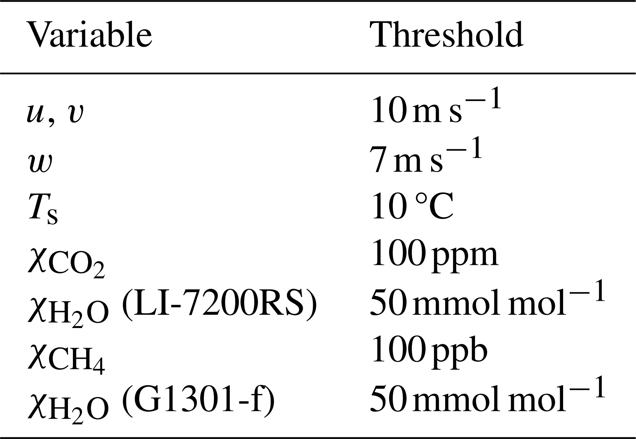
EC fluxes were calculated using the EddyUH software (Mammarella et al., 2016), following state-of-the-art methodologies (Sabbatini et al., 2018; Nemitz et al., 2018). Raw data were despiked based on the maximum difference allowed between two subsequent data points, according to the threshold values listed in Table 1. The dilution and spectroscopic correction (Chen et al., 2010) were point-by-point applied to the measured CH₄ mole fraction using the simultaneous H₂O mole fraction measured in the sampling cell of the Picarro analyser. The LI-7200RS internally corrects the water-induced density effect and gives as an output the dry mole fraction of CO₂. No density corrections were therefore needed for CO₂ (Burba et al., 2012). Although operated, the inclinometer data were not used for correcting the wind velocity components. It was checked from cospectra of $\stackrel{\mathrm{‾}}{u^{\prime }{w}^{\prime }}$ and $\stackrel{\mathrm{‾}}{v^{\prime }{w}^{\prime }}$ that the differences between the inclinometer-corrected and uncorrected velocities were only random. Instead, the inclinometer data were used for screening out the occasions when the movement of the platform was too large, i.e. when there were persons on the platform. A crosswind correction of sonic temperature was applied according to Liu et al. (2001). Additionally, a double coordinate rotation was applied to the sonic anemometer data by forcing the mean values of lateral (v) and vertical (w) velocity components of wind to zero.

Table 1 Threshold values for detecting spikes in different variables.

Gas fluxes were calculated from the covariance between the vertical wind speed w and the gas dry mole fraction χ, multiplied by the molar density of air ρ_a, as

$$\begin{array}{}\text{(1)}& F_{\mathit{\chi }}={\mathit{\rho }}_{\mathrm{a}}\stackrel{\mathrm{‾}}{w^{\prime }{\mathit{\chi }}^{\prime }},\end{array}$$

where the overbar denotes the time average and the prime the deviation from the mean. An averaging time of 30 min was used. The time series were linearly detrended so that the turbulent fluctuation in Eq. (1) was defined as the deviation from the linear trend. By definition, a positive flux indicates an upward flux (from the surface to the atmosphere).

Before calculating the covariance, the time lag between w and χ was removed. The time lag was determined by finding the maximum of the cross-covariance of w and χ within a given lag window (Aubinet et al., 2000). Examples of cross-covariance functions are shown in Fig. 2. Due to the low signal-to-noise ratio and in order to reduce the possible mirror effect of the fluxes around zero (Kohonen et al., 2020), a constant lag of 0.34 s was used for CO₂ and 7.0 s for CH₄. These values were calculated as the mean values of the estimated time lag distribution which remained well concentrated around the constant values throughout the campaign and did not experience drift (Fig. S1 in the Supplement). For H₂O, a relative humidity (RH)-dependent time lag, varying from 0.30 to 1.8 s, was used in order to account for the H₂O sorption in the sample line.

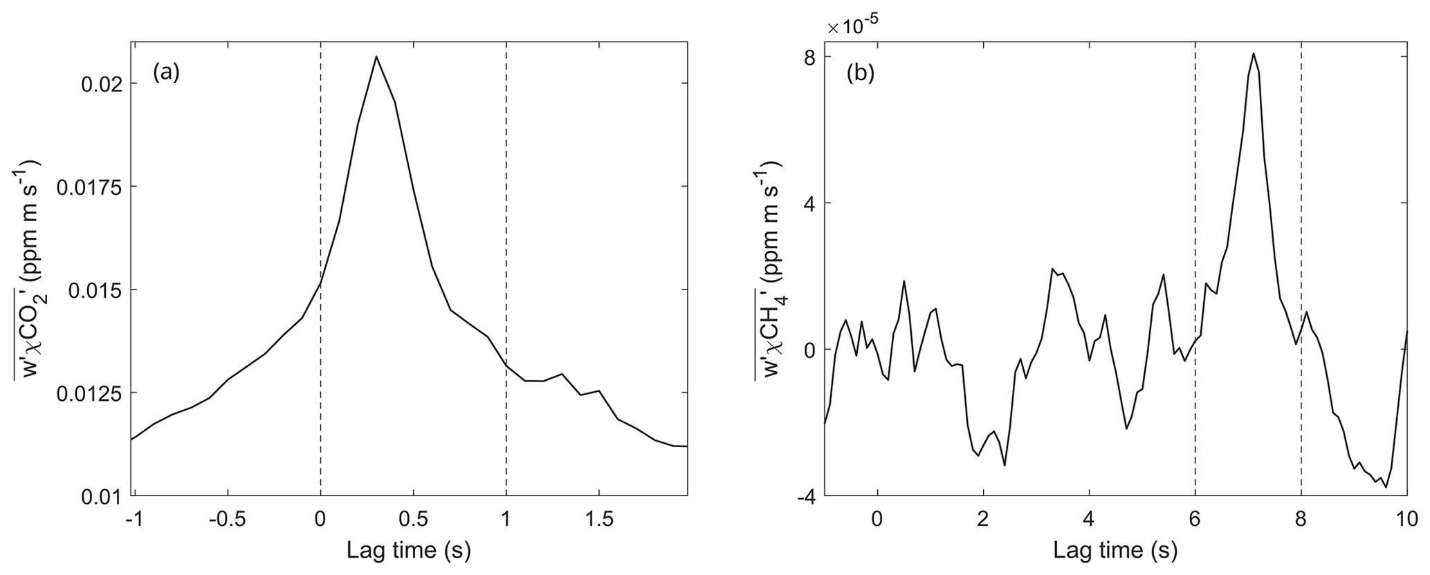
Figure 2 Example cases of maximising the cross-covariance between (a) CO₂ and w and (b) CH₄ and w. The dashed lines mark the boundaries between which the maximum was searched. In these cases, the location of the cross-covariance peak, i.e. the lag time for these particular averaging periods, was t_lag=0.3 s for CO₂ and t_lag=7.1 s for CH₄.

Fluxes were corrected for both low- and high-frequency attenuation. The actual unattenuated flux F is calculated from the measured flux F_χ as

$$\begin{array}{}\text{(2)}& F={\displaystyle \frac{F_{\mathit{\chi }}}{F_{\text{a}}}},\end{array}$$

where F_a is the flux attenuation. It is defined as the integral of a model cospectrum C_model(f) and the total transfer function TF, normalised by the model cospectrum:

$$\begin{array}{}\text{(3)}& F_{\text{a}}=\underset{\mathrm{0}}{\overset{\mathrm{\infty }}{\int }}{C}_{\text{model}}\left(f\right)\text{TF}\left(f\right)\text{d}f/\underset{\mathrm{0}}{\overset{\mathrm{\infty }}{\int }}{C}_{\text{model}}\left(f\right)\text{d}f.\end{array}$$

TF is a product of the high- and low-frequency transfer functions that describe the attenuation at different frequencies (f).

The low-frequency flux attenuation stems from the linear detrending of the original time series (Rannik and Vesala, 1999). The theoretical transfer function in this case is

$$\begin{array}{}\text{(4)}& \begin{array}{rl}{\text{TF}}_{\text{LF}}& =\mathrm{1}-{\displaystyle \frac{{\sin }^{\mathrm{2}}\left(\mathit{\pi }f{T}_{\text{av}}\right)}{{\left(\mathit{\pi }f{T}_{\text{av}}\right)}^{\mathrm{2}}}}\\ & -\mathrm{3}{\displaystyle \frac{{\left[\sin \left(\mathit{\pi }f{T}_{\text{av}}\right)-\mathit{\pi }f{T}_{\text{av}}\cos \left(\mathit{\pi }f{T}_{\text{av}}\right)\right]}^{\mathrm{2}}}{{\left(\mathit{\pi }f{T}_{\text{av}}\right)}^{\mathrm{4}}}},\end{array}\end{array}$$

where T_av is the averaging time. The high-frequency correction of fluxes was solved using an experimental transfer function (Aubinet et al., 2000). It is assumed that the temperature cospectrum C_wθ is unattenuated and therefore used as reference cospectrum. The measured transfer function is then

$$\begin{array}{}\text{(5)}& {\text{TF}}_{\text{meas}}={\displaystyle \frac{N_{\mathit{\chi }}{C}_{w\mathit{\chi },\text{meas}}}{N_{\mathit{\theta }}{C}_{w\mathit{\theta }}}},\end{array}$$

where N_χ and N_θ are normalisation factors equal to the covariances $\stackrel{\mathrm{‾}}{w^{\prime }{\mathit{\chi }}^{\prime }}$ and $\stackrel{\mathrm{‾}}{w^{\prime }{\mathit{\theta }}^{\prime }}$, respectively. The following functional form was then fitted to the measured values of Eq. (5):

$$\begin{array}{}\text{(6)}& {\text{TF}}_{\text{HF}}={\displaystyle \frac{\mathrm{1}}{{\left(\mathrm{1}+\mathrm{2}\mathit{\pi }f\mathit{\tau }\right)}^{\mathrm{2}}}},\end{array}$$

where τ is the response time. Similarly as with the lag time determination, the response time was not affected by sorption effects in the cases of CO₂ and CH₄ fluxes, and a constant response time τ=0.185 s for CO₂ and τ=0.2 s for CH₄ could be used. In contrast, τ for H₂O is relative-humidity-dependent (Mammarella et al., 2009). In this case, τ was determined by dividing the measured cospectra into six RH classes and calculating the bin mean. Then, a curve of the following form was used:

$$\begin{array}{}\text{(7)}& {\mathit{\tau }}_{{\text{H}}_{\mathrm{2}}\text{O}}=b_{\mathrm{1}}+b_{\mathrm{2}}(\mathrm{RH}/\mathrm{100}{)}^{b_{\mathrm{3}}},\end{array}$$

with $b_{\mathrm{1}}=-\mathrm{0.057}$, b₂=0.79 and b₃=1.6 fitted to the averaged data.

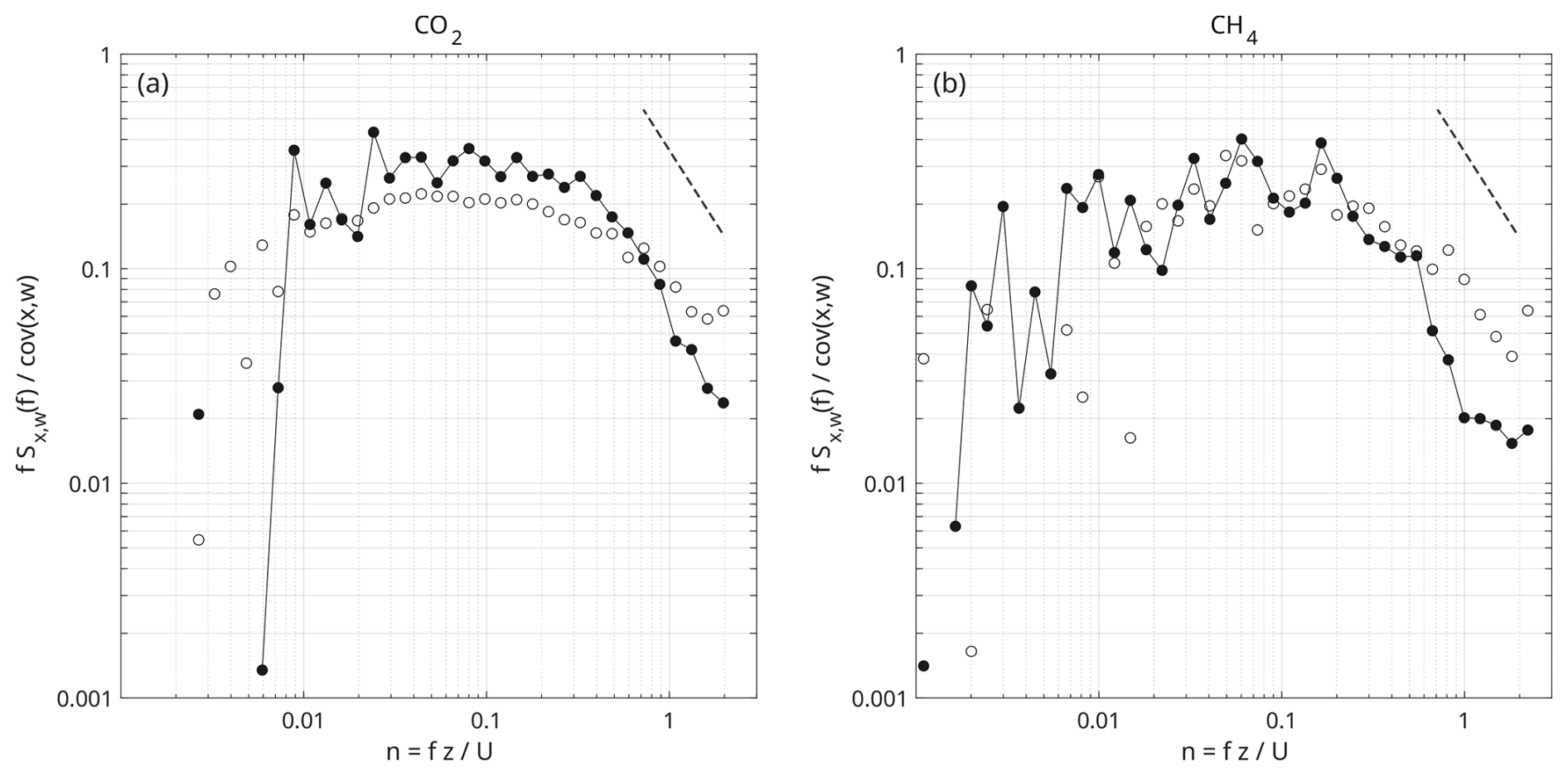
Figure 3 Mean normalised cospectra of (a) χCO₂ and w and (b) χCH₄ and w from 19–22 July when the fluxes were at their highest. The black circles represent the mean cospectra. The white circles are the mean normalised cospectra of the sonic temperature and w. The dashed lines show the $-\mathrm{4}/\mathrm{3}$ slope. The cospectra are presented by the normalised dimensionless frequency $n=fz/U$, where f is the natural frequency, z is the measurement height and U is the wind speed.

The model cospectrum in Eq. (3) was determined by fitting the function proposed by Kristensen et al. (1997) to the measured normalised temperature cospectrum C_wθ:

$$\begin{array}{}\text{(8)}& C_{\text{model}}\left(n\right)={\displaystyle \frac{a\cdot \frac{\mathrm{2}\mathit{\pi }}{z}n}{{\left[\mathrm{1}+{\left(\mathrm{2}\mathit{\pi }nL\right)}^{\mathrm{2}\mathit{\mu }}\right]}^{\mathrm{7}/\left(\mathrm{6}\mathit{\mu }\right)}}},\end{array}$$

where $n=zf/U$ is the normalised frequency, z is the measurement height and U is the mean wind speed. The fit parameters were a=6.78 m, L=1.35 and μ=0.32 for unstable cases and a=57.00 m, L=1.84 and μ=0.17 for stable cases.

Mean cospectra of CO₂ and CH₄ follow the theoretical shape and exhibit a well-defined inertial subrange (Fig. 3).

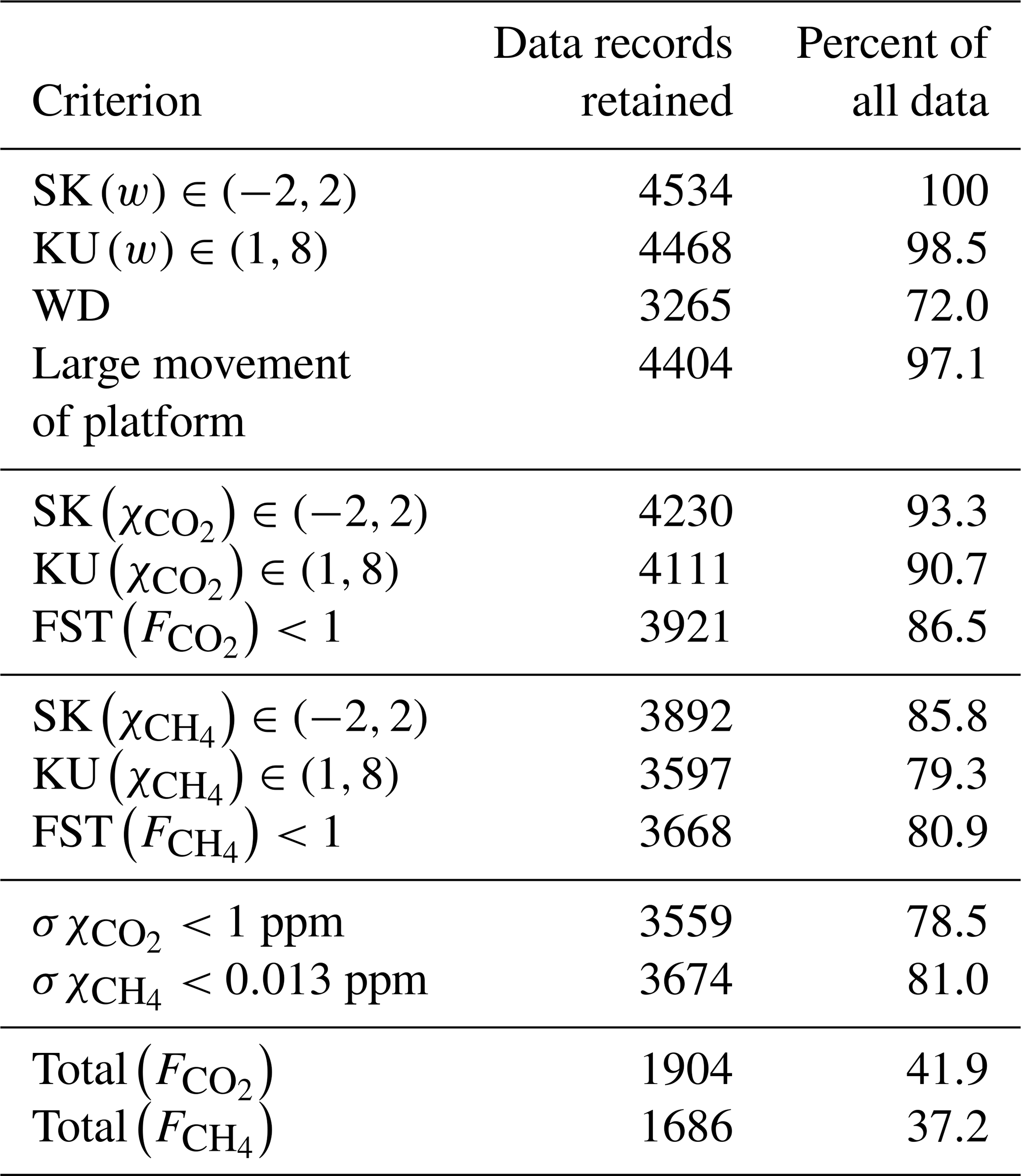
The following criteria were used in the post-processing quality control of the fluxes: skewness “SK” and kurtosis “KU” of both w and the dry mole fraction χ of the gas in question ($-\mathrm{2}<\mathrm{SK}<\mathrm{2}$, $\mathrm{1}<\mathrm{KU}<\mathrm{8}$) (Vickers and Mahrt, 1997); flux stationarity (FST≤1) (Foken and Wichura, 1996); the number of spikes (≤1800 in a 30 min averaging period); the wind direction; and occasions when the platform swayed too much, most often due to persons on the platform. As suggested by Erkkilä et al. (2018), additional filtering was done based on threshold values of standard deviation of carbon dioxide (${\mathit{\sigma }}_{{\mathit{\chi }}_{{\mathrm{CO}}_{\mathrm{2}}}}$) and methane (${\mathit{\sigma }}_{{\mathit{\chi }}_{{\mathrm{CH}}_{\mathrm{4}}}}$) mixing ratios. The criteria retained 30 min flux values when ${\mathit{\sigma }}_{{\mathit{\chi }}_{{\mathrm{CO}}_{\mathrm{2}}}}<\mathrm{1}\mathrm{ppm}$ and ${\mathit{\sigma }}_{{\mathit{\chi }}_{{\mathrm{CH}}_{\mathrm{4}}}}<\mathrm{0.013}\mathrm{ppm}$.

In order to find acceptable wind sectors, the flux footprint model by Kljun et al. (2015) was used. Parameters for the footprint calculation were the friction velocity u_*, standard deviation of lateral wind velocity σ_v, wind direction and the calculated Obukhov length L_MO. We assume a constant boundary layer height h_BL=1000 m and roughness length z₀=0.01 m. The full dataset of these variables was used in the footprint analysis. The determination of the roughness length is explained in detail in the Supplement, and the distribution of the observed values of z₀ is shown in Fig. S2. The resulting footprint climatology, depicted in Fig. 4, is roughly oval-shaped, with the long axis approximately along the river. Estimates for the footprint are generally not applicable with changing roughness; therefore, the river bank directions are excluded from further flux analysis. The longest distance to the 90 % footprint line at the southern side over the river is 177 m. Sectors where the river bank was further than 177 m from the platform were accepted. The two sectors are 123–181° and 285–355°.

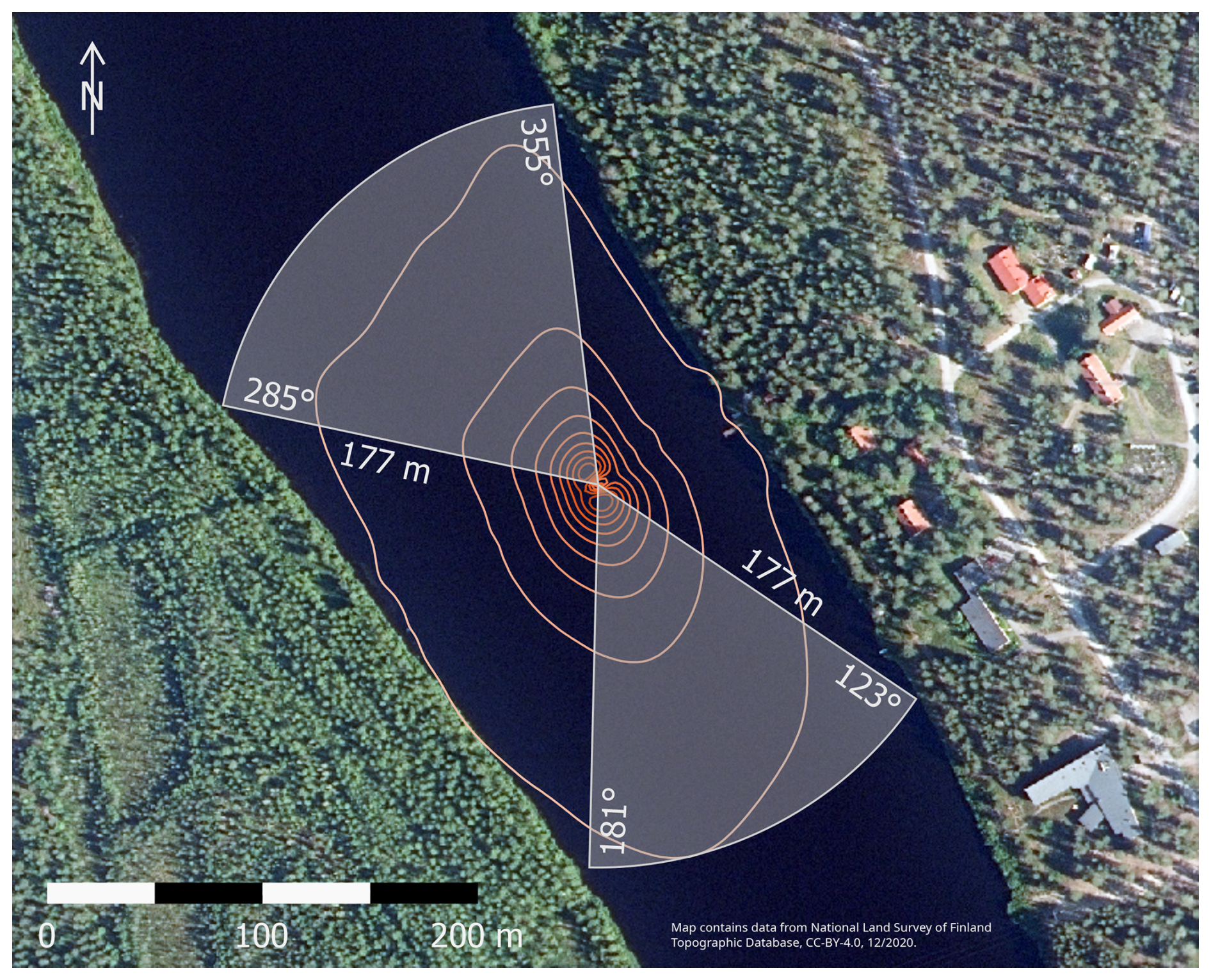
Figure 4 Flux footprint climatology. The curves show the footprint percentiles at 10 % intervals, starting from the outermost 90 % footprint. The grey sectors are the accepted wind directions.

However, there were numerous cases where the average 30 min wind direction was seemingly from an accepted sector, but the instantaneous wind direction was at least partly from a rejected sector. In some cases, this had a considerable effect on the measured concentration and flux values, as the surrounding land was a source or sink of carbon dioxide, depending on the time of the day, as well as a source of methane. In addition, the magnitude of these sources or sinks can be larger than in the river. An example of such a case is shown in Fig. A1 when an air mass from the land caused an abrupt increase in the CO₂ mixing ratio and a decrease in temperature after 23:53 UTC. In this case, the stationarity value of the CO₂ flux was 0.35; i.e. it passed the criterion FST<1. To mitigate this effect, the following approach was used. Fluxes were calculated for 5 min subintervals. If the mean wind direction fell within the accepted sectors in all of the six subintervals, the corresponding 30 min flux value was retained. If more than one but less than six subintervals fell within the accepted sectors, their average was used as the value for the flux for that 30 min record. The record with one or no accepted 5 min subintervals was discarded. This method still potentially leaves intermittent periods of wind from land for less than 5 min in the accepted data but reduces their amount and their contribution to the final fluxes. Evidently, when the average of the 5 min fluxes was used, it is a better approximation of the river surface exchange than the corresponding 30 min flux as the difference between the 30 min fluxes and the averaged 5 min fluxes reduces with an increasing number of averaged 5 min intervals (Fig. A2).

After the flux calculation and the raw data quality control, there were altogether 4534 data records of 30 min fluxes. Table 2 summarises all flux quality control criteria and how much of the original 30 min data were retained after applying the criteria. In total, 43.9 % of the original $F_{{\mathrm{CO}}_{\mathrm{2}}}$ records and 38.9 % of the original $F_{{\mathrm{CH}}_{\mathrm{4}}}$ records remained after the quality control. Wind direction and standard deviation of gas-mixing ratios were the most prominent criteria, and they removed approximately one-fourth and one-fifth of all the data, respectively. Most of the applied criteria overlapped with each other.

Table 2 The applied post-processing quality criteria and the amount of data they retain. SK: skewness; KU: kurtosis; WD: wind direction; FST: flux stationarity.

2.4 Ancillary measurements and data processing

Ambient air temperature (T_a) and relative humidity were measured with a Rotronic HC2-S3C03 probe (Rotronic AG, Bassersdorf, Germany), mounted inside a Young model 41003 (R. M. Young Company, Traverse City, Michigan, USA) multi-plate radiation shield on the platform's north-eastern corner. T_a and RH were available only after 15 June. Before that, the sonic temperature and humidity calculated from ${\mathit{\chi }}_{{\mathrm{H}}_{\mathrm{2}}\mathrm{O}}$, measured with the LI-7200RS, were used instead. Atmospheric pressure p_atm and precipitation were measured at the Tähtelä weather station. Photosynthetically active radiation (PAR) in water was measured with two LI-192 and one LI-193 sensors (LI-COR Biosciences, Inc., Lincoln, Nebraska, USA). The sensors were hanging from wires at 0.3 and 1.0 m depths (LI-192) and at 0.65 m (LI-193) on a beam on the southern side of the platform. In the analysis, we used the sensor at 0.3 m.

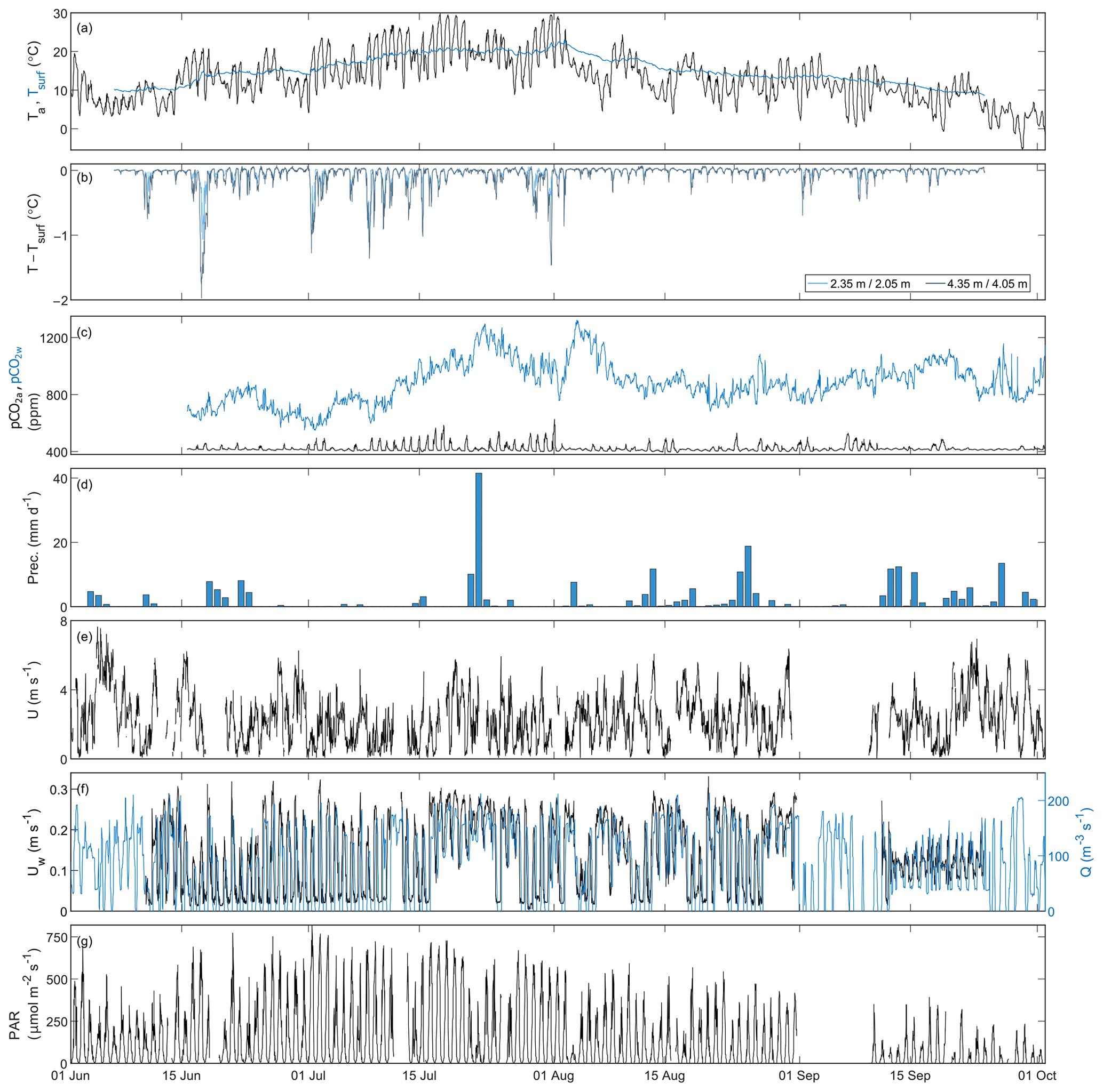
Figure 5 Environmental conditions during the campaign. The variables are shown as 30 min average values, except for the precipitation data, which are shown as daily values. (a) Air temperature 2 m above river surface T_a (black) and water surface temperature T_surf (blue). (b) Deviation of the water temperature at 2.35 m/2.05 m and 4.35 m/4.05 m (bottom) from the surface temperature. (c) Atmospheric CO₂ partial pressure $p{{\mathrm{CO}}_{\mathrm{2}}}_{\text{a}}$ (black) measured 0.4 m above the water surface and surface water CO₂ partial pressure $p{{\mathrm{CO}}_{\mathrm{2}}}_{\text{w}}$ (blue). (d) Daily precipitation. (e) Wind speed U. (f) Water flow speed U_w (left, black) and discharge Q (right, blue). (g) Photosynthetically active radiation (PAR) at 0.30 m depth. Discharge was measured 11 km downstream. Precipitation was measured at the Tähtelä weather station.

Measurements of waterside CO₂ partial pressure ($p{{\mathrm{CO}}_{\mathrm{2}}}_{\text{w}}$) were done by using an off-axis integrated cavity output spectrometer (ultraportable greenhouse gas analyser (UGGA), Los Gatos Research, Inc., Santa Clara, California, USA) that was connected to the headspace of an equilibrator consisting of a floating Plexiglas chamber ($\mathrm{130}\times \mathrm{500}\times \mathrm{500}$ mm) sticking about 50 mm into the water, leaving a headspace volume of about 20 L. The air in the headspace was circulated through the UGGA in a closed loop where the intake tube was fitted with a membrane (ACCUREL polypropylene capillary membrane, Membrana GmbH, Germany) that prevented water from entering the UGGA. In order to increase the response time of the equilibrium concentration, a diffuser was placed in the water about 30 mm below the surface just beneath the chamber. The diffuser consisted of a disc covered by a membrane with a large number of small holes. An external pump forced the air from the headspace through the diffuser at a rate of 2.5 L min⁻¹. A laboratory test showed that the time response of the system was about 40 min for 95 % change in concentration. The UGGA was connected to the equilibrator during 5 min every 20 min. The first 2 min after connection was skipped to allow the gas analyser to adapt to the new conditions (ambient air concentrations at 0.40 and 2.40 m above the water surface were also monitored with the same system), allowing 3 min for averaging. The UGGA was calibrated against reference gases (562–1188 ppm CO₂) with a specified accuracy of 2 %.

A water temperature chain was set up 100 m upstream of the platform. It consisted of five temperature loggers of the type RBR Solo (RBR Ltd, Ottawa, Ontario, Canada). The loggers were placed on a taut line mooring at depths of 0.35, 1.35, 2.35, 3.35 and 4.35 m (6 to 17 June) and 0.07, 1.05, 2.05, 3.05 and 4.05 m (17 June onwards). The topmost measurement was used as the surface temperature. The water flow velocity was measured with an acoustic Doppler velocimeter (Nortek Vector, Nortek AS, Rud, Norway), which was installed on a beam on the north-western corner of the platform, facing down (Guseva et al., 2021). The depth of the measurements was 0.4 m below the surface.

Spikes in ancillary data were identified with a MATLAB Hampel filter. The filter uses a moving window and identifies outliers with a standard deviation criterion. The filter parameters were hand-tuned for each variable. Spikes were replaced with linearly interpolated values.

Figure 6 Wind climatology during the campaign.

2.5 Multiple regression analysis

To study the drivers of the gas exchange, multiple linear regression between the fluxes and their possible drivers were tested. The driving variables were T_surf, PAR, wind speed (U), water flow speed (U_w), $p{{\mathrm{CO}}_{\mathrm{2}}}_{\text{w}}$ and precipitation (prec). All fluxes and environmental variables were distributed normally at a 95 % confidence level, thus making it possible to use regression models. Regressions were calculated on 24 h and 7 d timescales, chosen to average diel and synoptic variations. Averages were accepted when the data coverage was more than 30 %. Outliers in the averages were removed before calculating the regression models. The model results were ranked by the adjusted coefficient of determination $R_{\text{adj}}^{\mathrm{2}}$. The adjusted R² was used instead of the ordinary R² to account for the artificial inflation of R² when more variables are added to a model.

Due to intercorrelation among the driving variables themselves, similar multiple regression calculations were also conducted for $p{{\mathrm{CO}}_{\mathrm{2}}}_{\text{w}}$ with water temperature, PAR, precipitation, wind speed and water flow speed as the driving variables.

Additionally, the dependence of the diurnal variability of $p{{\mathrm{CO}}_{\mathrm{2}}}_{\text{w}}$, $F_{{\mathrm{CO}}_{\mathrm{2}}}$ and $F_{{\mathrm{CH}}_{\mathrm{4}}}$ on the drivers was tested similarly as with the 1 and 7 d means. In calculating the cycles, the mean of each individual day was first subtracted in order to analyse only the daily variability and not the longer-term changes in the baseline of the variables. The same driving variables were used in these calculations, except for precipitation for which there were only daily values available. All of the driving variables exhibited diurnal variability.

3 Results

3.1 Environmental conditions

The 30 min average air temperature rose from 10 °C at the beginning of the campaign to 30 °C in early August and then fell slightly below the freezing point towards the end of the campaign (Fig. 5a). The river surface temperature was 10 °C at the start of the campaign, reached its maximum value of 21.9 °C in the beginning of August and then fell close to the freezing point towards the end of the campaign (Fig. 5a), following closely the seasonal variation of air temperature. The water temperature difference between the river surface and the bottom was less than 2.0 °C at any time during the campaign (Fig. 5b). Stratification, defined as when the temperature difference between surface and bottom exceeded 0.05 °C, occurred when the flow was reduced, during 38 % of the campaign (Guseva et al., 2021).

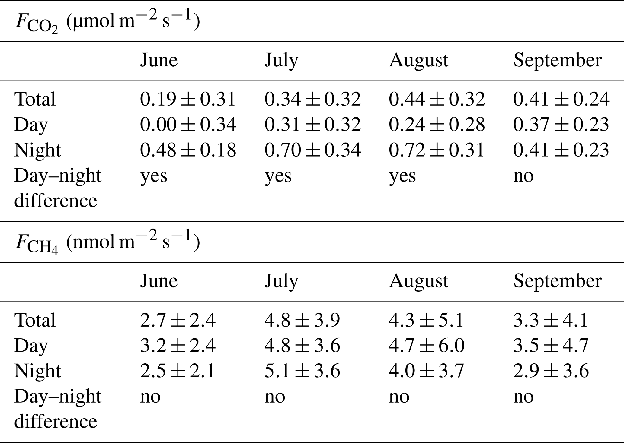
Table 3 Mean fluxes and their standard deviation in each month during the campaign and the overall mean fluxes. The mean fluxes and the standard deviation are also shown for daytime and nighttime during each month. The day–night difference indicates whether there was a statistically significant difference in the fluxes between day and night.

The surface water at the platform was constantly supersaturated with CO₂ with respect to the atmosphere (Fig. 5c). The CO₂ partial pressure in the water pCO₂w varied between 550 and 1323 ppm, the lowest values occurring in June and the highest in July. The daily variation of pCO₂w ranged from 5 to 225 ppm.

The monthly precipitation was 43.7 mm in June, 61.4 mm in July, 75.9 mm in August and 78.5 mm in September–October (Fig. 5d). These correspond to approximately 25 % less than the average precipitation in June and July and about 40 % and 50 % more than average in August and September, respectively. In July, there was one heavy rain event that brought 41.5 mm of precipitation during a single day.

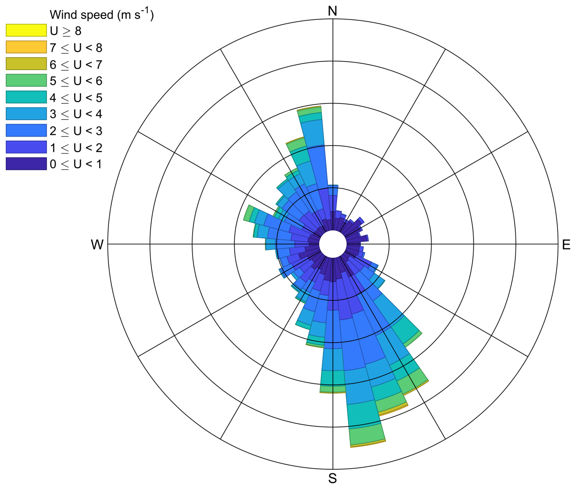
The 30 min mean wind speed varied between 0 and 8 m s⁻¹ during the campaign months (Fig. 5e). The wind speed had both diurnal and synoptic variations and was largely channelled along the river (Fig. 6). The water flow speed varied from 0 to 0.33 m s⁻¹ (Fig. 5f), showing as well a diel pattern due to the downstream dam operation (Guseva et al., 2021). Finally, underwater PAR measurements showed expected diurnal and seasonal variations (Fig. 5g), with the largest daytime values recorded in July (760 µmol m⁻² s⁻¹) and the lowest at the end of the field campaign in September (60 µmol m⁻² s⁻¹). The net radiation (Fig. S3a) had also distinct diurnal and seasonal variability, as did PAR at all the measured depths (Fig. S3b).

3.2 CO₂ and CH₄ fluxes

The quality-controlled 30 min fluxes of CO₂ and CH₄ as well as their daily-averaged values are shown in Fig. 7. Both $F_{{\mathrm{CO}}_{\mathrm{2}}}$ and $F_{{\mathrm{CH}}_{\mathrm{4}}}$ had a moderate seasonal variability, showing higher fluxes in July and August. The monthly-mean $F_{{\mathrm{CO}}_{\mathrm{2}}}$ values (standard deviation) were 0.19 (SD 0.31) (in June), 0.34 (SD 0.32) (in July), 0.44 (SD 0.32) (in August) and 0.41 µmol m⁻² s⁻¹ (SD 0.24 µmol m⁻² s⁻¹) (in September). The mean $F_{{\mathrm{CO}}_{\mathrm{2}}}$ during the entire campaign was 0.36 µmol m⁻² s⁻¹ (SD 0.31 µmol m⁻² s⁻¹). The monthly-mean fluxes are presented in Table 3.

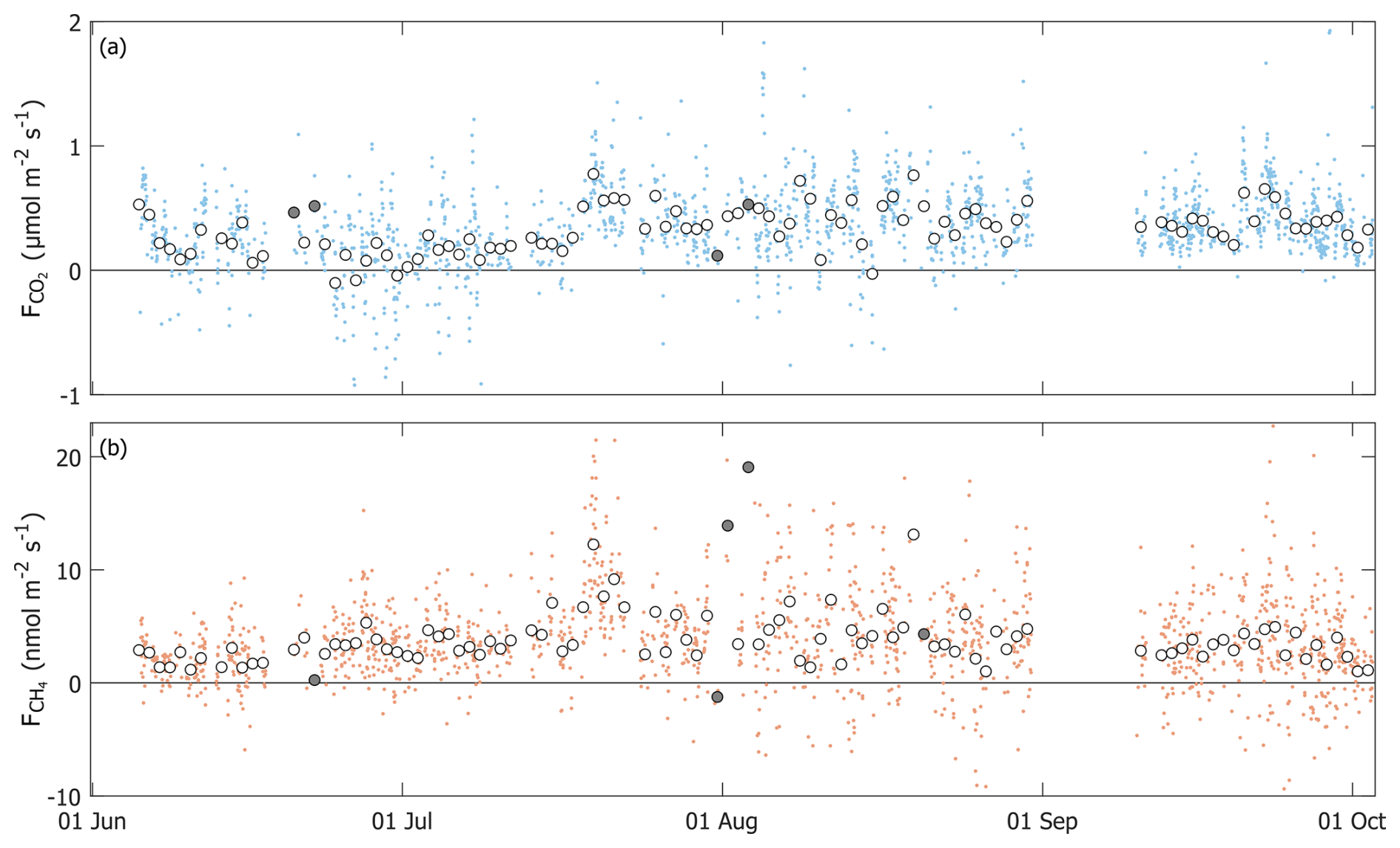
Figure 7 Time series of the CO₂ (a) and CH₄ fluxes (b). The dots indicate the 30 min values, and the circles indicate the daily averages. Fluxes are quality-controlled. The daily fluxes are drawn with a dark circle if the day contained only three or fewer 30 min fluxes.

The variability of $F_{{\mathrm{CO}}_{\mathrm{2}}}$ was larger at nighttime compared to daytime during all months (Fig. 8, left panel). Performing a two-sample t test on $F_{{\mathrm{CO}}_{\mathrm{2}}}$ during daytime and nighttime (09:00–15:00 and 21:00–03:00 LT (local time), respectively) in different months, there is also a statistically significant difference (p<0.05) between the daytime and nighttime fluxes during June, July and August. In other words, during those months there was diurnal variation in the fluxes, with the nighttime fluxes being higher. In September, however, such variation did not exist. The mean nighttime $F_{{\mathrm{CO}}_{\mathrm{2}}}$ (0.25 µmol m⁻² s⁻¹) in June–September was 220 % of the mean daytime $F_{{\mathrm{CO}}_{\mathrm{2}}}$ (0.55 µmol m⁻² s⁻¹). The day–night difference in $F_{{\mathrm{CO}}_{\mathrm{2}}}$ was significant when observing the entire campaign's duration. Table 3 also contains the daytime and nighttime mean fluxes.

The monthly-mean $F_{{\mathrm{CH}}_{\mathrm{4}}}$ values (standard deviation) were 2.7 (SD 2.4) (June), 4.8 (SD 3.9) (July), 4.3 (SD 5.1) (August) and 3.3 nmol m⁻² s⁻¹ (SD 4.1 nmol m⁻² s⁻¹) (September). The mean $F_{{\mathrm{CH}}_{\mathrm{4}}}$ during the campaign was 3.8 nmol m⁻² s⁻¹ (SD 4.1 nmol m⁻² s⁻¹). Contrary to $F_{{\mathrm{CO}}_{\mathrm{2}}}$, there was no statistically significant diurnal variation in $F_{{\mathrm{CH}}_{\mathrm{4}}}$ during any month of the campaign (Fig. 8, right panel). The measured nighttime $F_{{\mathrm{CH}}_{\mathrm{4}}}$ (3.3 nmol m⁻² s⁻¹) in June–September was 80 % of the daytime flux (4.1 nmol m⁻² s⁻¹).

There was a period of relatively high fluxes during 19–25 July. The daily mean CO₂ fluxes reached 0.55–0.7 µmol m⁻² s⁻¹, and CH₄ fluxes reached 7–12 nmol m⁻² s⁻¹. This period coincided with the discharge being constantly kept above 100 m³s⁻¹ and with the daily average winds being higher than during other times in July.

3.3 Relationship between the fluxes and environmental drivers

All possible combinations of the driving variables were tested, but here we present the five best models in each case. The models shown are statistically significant at a 95 % confidence level. There was intercorrelation between almost all driving variables, but the coefficient of determination was mostly low.

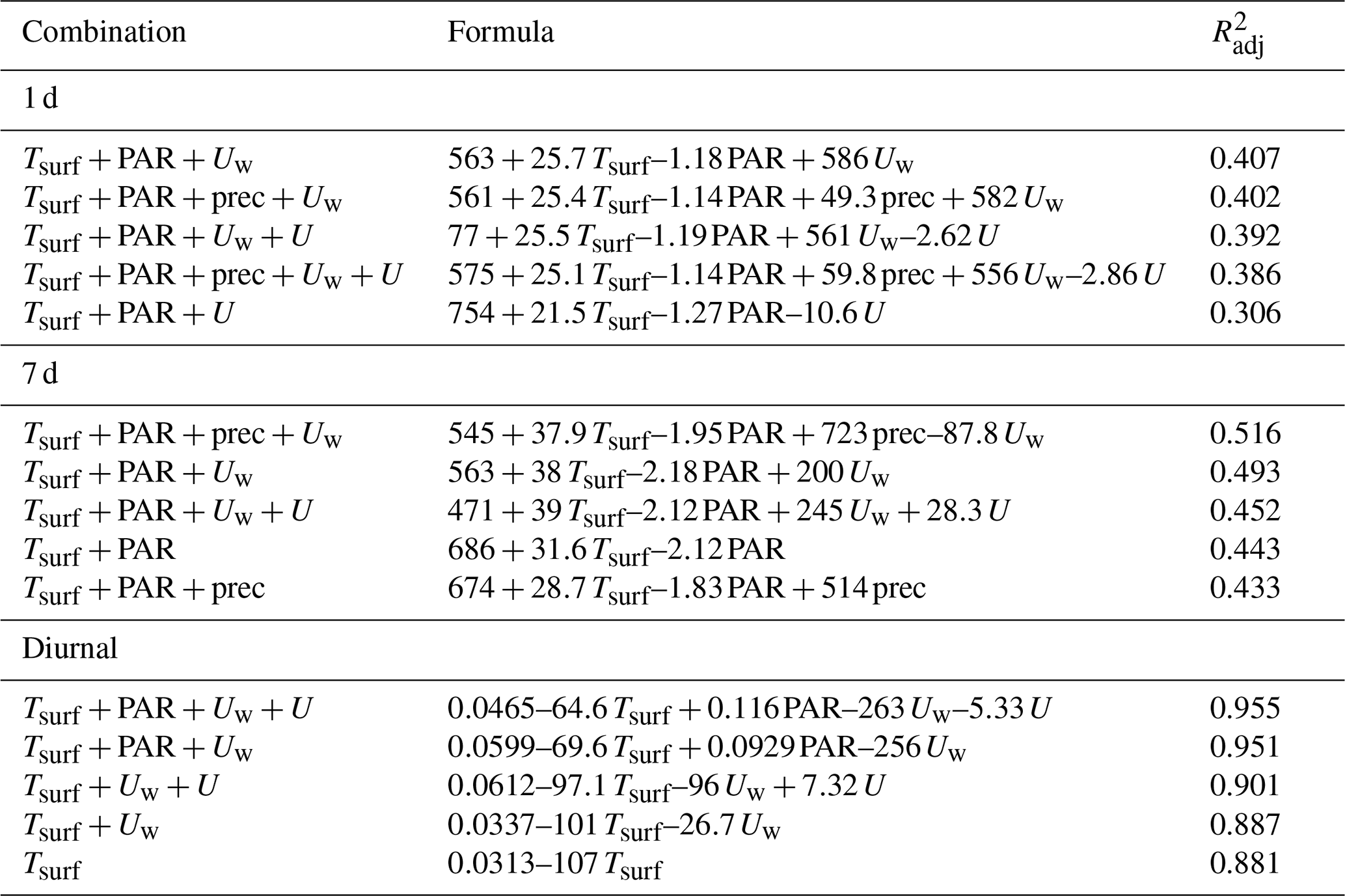
The best models for $p{{\mathrm{CO}}_{\mathrm{2}}}_{\text{w}}$ are similar at daily and weekly timescales (Table 4). $p{{\mathrm{CO}}_{\mathrm{2}}}_{\text{w}}$ was mainly driven by T_surf, PAR and U_w. Three of the best daily models include U. The response to T_surf and U_w was positive, while it was negative for PAR. An exception is the negative response to U_w in the best weekly model. This model also includes precipitation as a driver. The adjusted coefficient of determination, $R_{\text{adj}}^{\mathrm{2}}$, was 0.407 and 0.516 for the best daily and best weekly models, respectively. The diurnal cycle of $p{{\mathrm{CO}}_{\mathrm{2}}}_{\text{w}}$ correlated mainly with T_surf with a negative response, as it appears in all five best models. The four highest-ranking models also incorporate U_w as a driver with a negative response. $R_{\text{adj}}^{\mathrm{2}}$ is very high, 0.955, for the best model. Contrary to the daily and weekly means, only two models for the diurnal variability incorporated PAR as a driver; additionally, the response of $p{{\mathrm{CO}}_{\mathrm{2}}}_{\text{w}}$ to PAR was positive with the multiplier being close to 0.

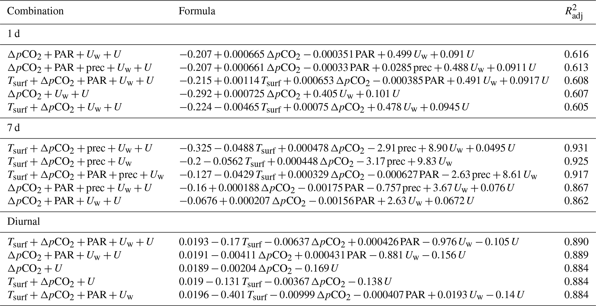
The best regression model for the CO₂ fluxes on a daily timescale contains ΔpCO₂, PAR, U_w and U (Table 5). The coefficient between these variables and $F_{{\mathrm{CO}}_{\mathrm{2}}}$ is positive except for PAR. Two models with the second best $R_{\text{adj}}^{\mathrm{2}}$ value also include precipitation or T_surf as additional explanatory variables. The explanatory variables ΔpCO₂, U_w and U appear in all five of the best models. The best model on a weekly timescale contains most of the selected environmental parameters, except PAR, which appears in the last three best models with a negative response. The four highest-ranking models also contain precipitation. $R_{\text{adj}}^{\mathrm{2}}$ was 0.621 for the best daily model and 0.928 for the best weekly model. The models' response to ΔpCO₂, U_w and U was positive at both weekly and daily timescales, while the response to PAR was always negative. The models had variable responses to T_surf and precipitation.

The diurnal variability in $F_{{\mathrm{CO}}_{\mathrm{2}}}$ was mainly driven by ΔpCO₂ as it appears in all five models. Additionally, U is present in four out of five of the best models. The response of $F_{{\mathrm{CO}}_{\mathrm{2}}}$ to these variables was negative. $R_{\text{adj}}^{\mathrm{2}}$ for the diurnal variability models was rather high, 0.89.

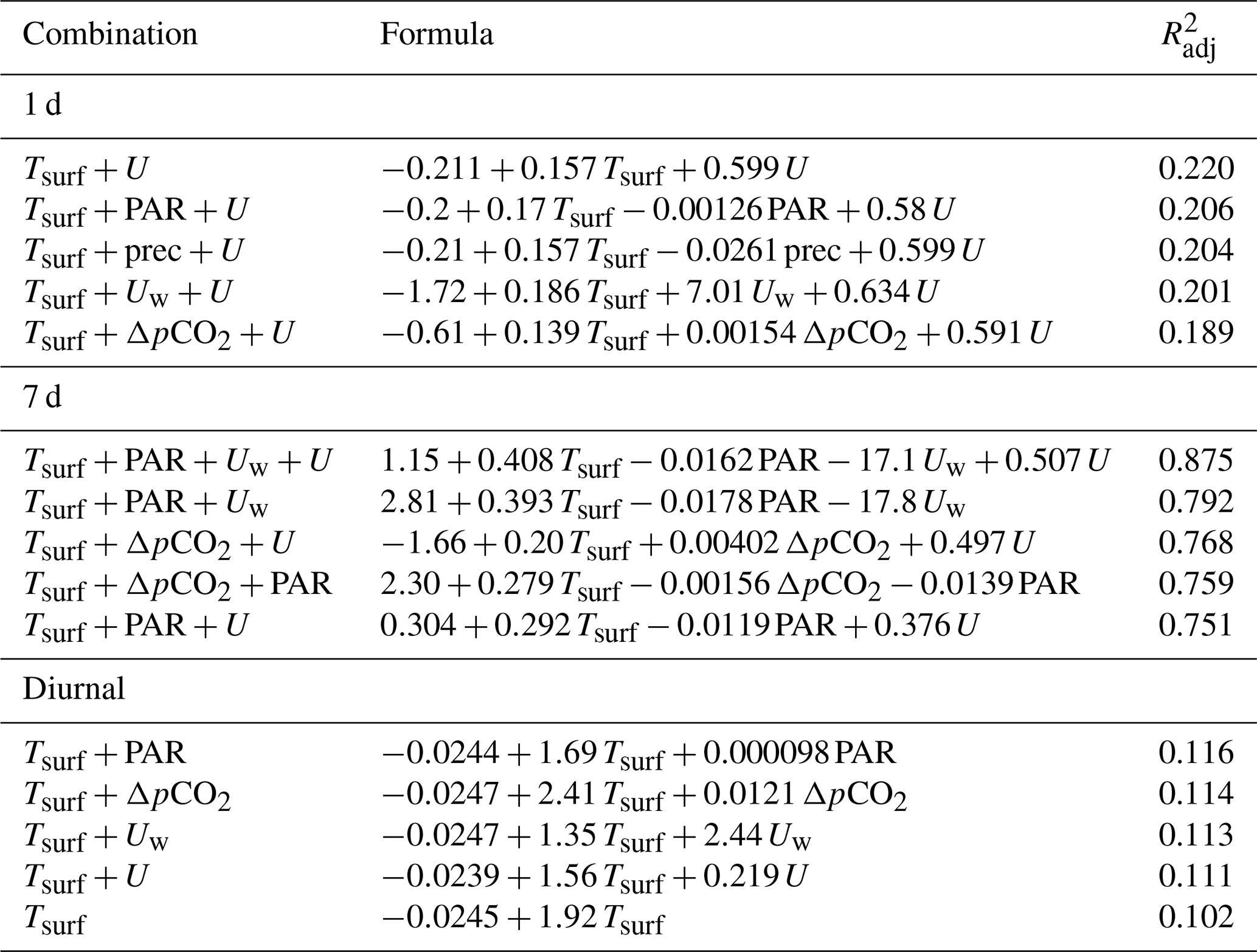
The best models for CH₄ fluxes on both daily and weekly timescales all contain T_surf, and the fluxes' response to T_surf is positive. The best models on a daily timescale additionally contain U. On the weekly timescale, most of the best models also include PAR. $R_{\text{adj}}^{\mathrm{2}}$ is only 0.19–0.22 on a daily timescale due to the large scatter in the data. On a weekly timescale, $R_{\text{adj}}^{\mathrm{2}}$ is high because the amount of weekly data was small. The diurnal variability was mainly driven by T_surf with a positive response, but $R_{\text{adj}}^{\mathrm{2}}$ is very low, i.e. only 0.12 in the best model.

Table 4 Multivariate linear regression models between the partial pressure of CO₂ in water ($p{{\mathrm{CO}}_{\mathrm{2}}}_{\text{w}}$ [µatm]) and surface temperature (T_surf [°C]), photosynthetically active radiation (PAR [µmol m⁻² s⁻¹]), wind speed (U [m s⁻¹]), precipitation (prec [mm d⁻¹]) and water flow speed (U_w [m s⁻¹]) that give the highest value of $R_{\text{adj}}^{\mathrm{2}}$ at timescales (averaging periods) of 24 h and 7 d, as well as averaged into a diurnal cycle. The Wilkinson notation is used in describing the combination of the variables. In the model formula, the unit of the intersection is microatmosphere (i.e. µatm), and the units of the variables' multipliers are microatmospheres divided by the unit of the variable, i.e. µatm / [unit of variable]. Only statistically significant models are shown.

4 Discussion

4.1 Challenges of EC flux measurements over a river

The EC technique is widely used for continuous and long-term monitoring of energy and gas exchanges between land ecosystems (forest, wetland, arable land, grassland) and atmosphere (Baldocchi, 2003). The method has been applied only recently to inland aquatic ecosystems, and at the moment there is no comprehensive network of long-term EC sites covering different latitudes, climatic zones or water body characteristics. Most of the previous EC studies over inland water bodies have focused on lakes and their water–atmosphere energy exchange, while only a few studies have reported direct EC fluxes of CO₂ and CH₄ over lakes (Mammarella et al., 2015; Czikowsky et al., 2018; Eugster et al., 2020; Golub et al., 2023). So far, only one study has reported CO₂ fluxes measured by the EC technique over a river (Huotari et al., 2013). While land-based EC flux measurements and data processing chains are well established (Sabbatini et al., 2018; Nemitz et al., 2018), standard EC data processing steps are not always applicable for measurements over inland water bodies. Fluxes are often smaller in magnitude than those typically found over land, and the reduced turbulent mixing over a smooth water surface may lead to further limitations during calm or moderate wind conditions (Spank et al., 2020), when the advection of gases from land also poses a problem for the EC flux measurements, i.e., not representing the surface gas exchange in these cases.

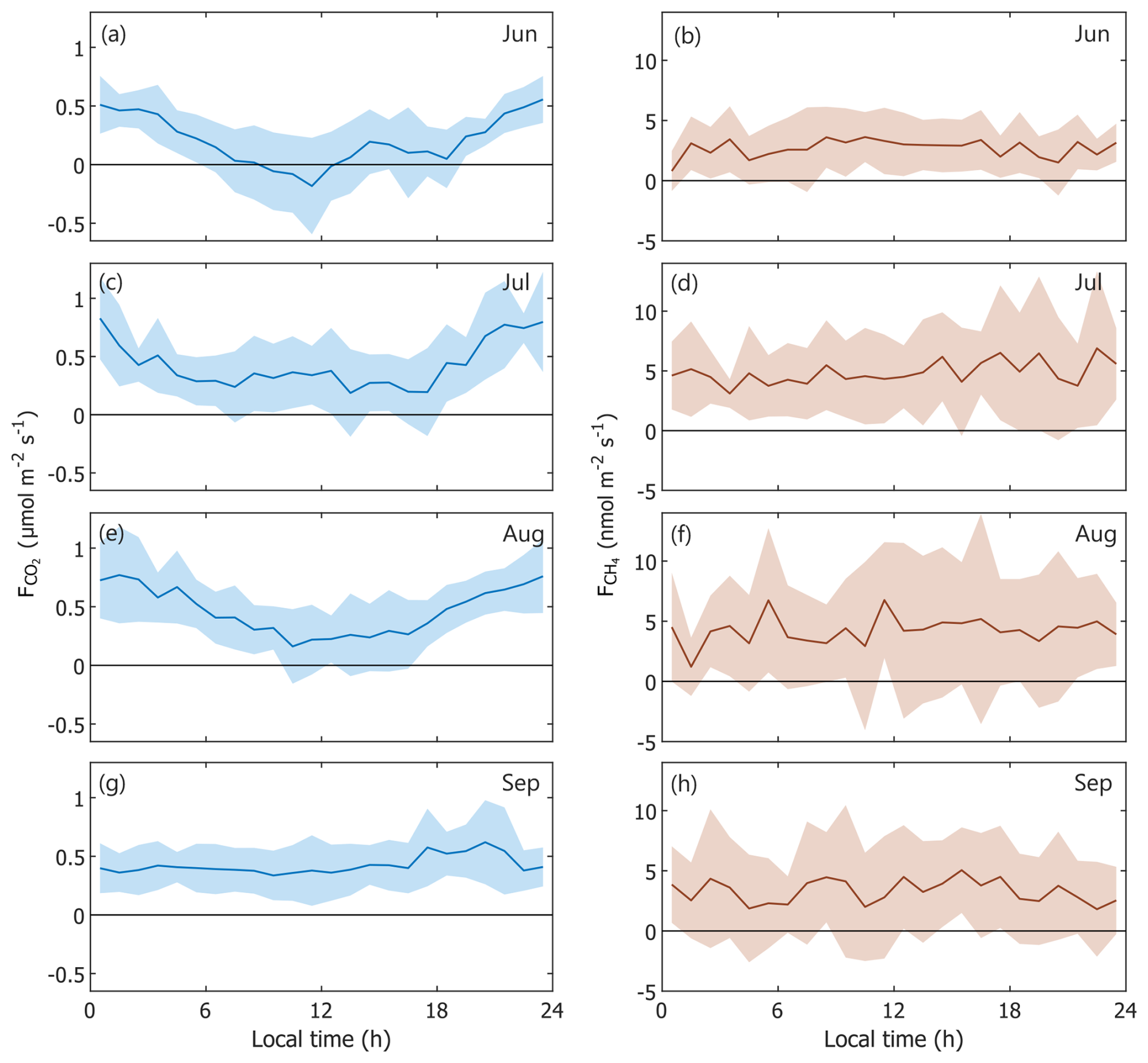
Figure 8 Diurnal variation of CO₂ flux (a, c, e, g) and CH₄ flux (b, d, f, h) in different months, averaged in 1 h bins. The line and the shaded area indicate the mean flux and its standard deviation, respectively.

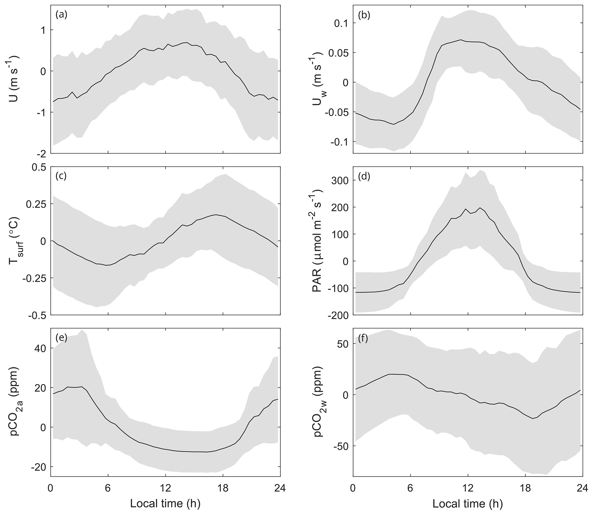
Figure 9 Mean diurnal cycles of the flux drivers, calculated by first subtracting the daily mean from each individual day. The line and the shaded area mark the mean and standard deviation, respectively. (a) Wind speed. (b) Flow speed. (c) Surface temperature. (d) Photosynthetically active radiation at 0.30 m depth. (e) CO₂ mixing ratio in air. (f) CO₂ mixing ratio in surface water.

Standard low-turbulence filtering criteria, based on friction velocity or standard deviation of the vertical component of wind velocity, are not recommended for EC fluxes over lakes and rivers, as the wind-shear-generated turbulence is one of the main drivers of gas exchange at the water–air interface. Here, we have proposed the method of dividing the 30 min intervals into shorter 5 min subintervals, which reveals how short-term changes in wind directions may contaminate the measured CO₂ signal, affecting the quality of measured 30 min fluxes (Fig. A2). Removing these situations when the flux signal originates from land makes the measured flux closer to an unbiased estimate of the gas exchange between the water surface and the atmosphere.

A few different approaches have been proposed for filtering low-turbulence and/or advection-dominated conditions, based on, for example, a minimum threshold value for the atmospheric stability (Czikowsky et al., 2018), a maximum threshold for the standard deviation of atmospheric CO₂ mixing ratio (Erkkilä et al., 2018), or thresholds for the trend $\text{d}\mathit{\chi }/\text{d}t$ and for the horizontal turbulent flux $\stackrel{\mathrm{‾}}{u^{\prime }{\mathit{\chi }}^{\prime }}$ of the compound (Blomquist et al., 2012). The choice of threshold values for stability, friction velocity or gas-mixing ratio is a mostly empirical, partly arbitrary and often site-specific choice. Despite our new wind subinterval filtering method, we still had to implement a screening based on maximum threshold values of standard deviation of gas-mixing ratios. This demonstrates the challenges in and importance of finding the correct criteria for the data screening. Still, verification of the turbulent exchange coefficients of heat and momentum for the cases with accepted fluxes (Figs. S4–S5) shows that the contribution from land to the quality-screened fluxes is negligible. In addition, the filtering successfully removed the cases of very stable atmospheric stratification during all times of the day (Figs. S6–S7).

Table 5 Multivariate linear regression models between CO₂ fluxes and surface temperature (T_surf [°C]), CO₂ partial pressure difference between water and air (ΔpCO₂ [µatm]), photosynthetically active radiation (PAR [µmol m⁻² s⁻¹]), wind speed (U [m s⁻¹]), precipitation (prec [mm d⁻¹]) and water flow speed (U_w [m s⁻¹]) that give the highest value of $R_{\text{adj}}^{\mathrm{2}}$ at timescales (averaging periods) of 24 h and 7 d, as well as averaged into a diurnal cycle. The Wilkinson notation is used in describing the combination of the variables. In the model formula, the unit of the intersection is µmol m⁻² s⁻¹, and the units of the variables' multipliers are µmol m⁻² s⁻¹ / [unit of variable]. Only statistically significant models are shown.

4.2 Magnitude and temporal dynamics of fluxes

So far, only Huotari et al. (2013) have reported EC CO₂ fluxes over a river. Measurements were carried out for about 1 month in summer 2009 at Kymijoki (southern Finland), which is a wider river than the river Kitinen and has a mean annual discharge that is 2.7 times as large as that of Kitinen, resulting in a higher water flow velocity ranging between 0.15 and 1.17 m s⁻¹, with a mean value of 0.66 m s⁻¹ (Huotari et al., 2013). The mean $F_{{\mathrm{CO}}_{\mathrm{2}}}$ over Kymijoki during their measurements was 0.94 ± 0.5 µmol m⁻² s⁻¹, which is 2.5 times as high as $F_{{\mathrm{CO}}_{\mathrm{2}}}$ over Kitinen during the KITEX campaign. Huotari et al. (2013) attributed changes in the measured flux to changes in pCO₂ in the water, which in turn was negatively correlated with discharge. Contrary to this study, Huotari et al. (2013) did not detect any significant diurnal cycle in $F_{{\mathrm{CO}}_{\mathrm{2}}}$. They measured $p{{\mathrm{CO}}_{\mathrm{2}}}_{\text{w}}$ to be approximately 600–1000 µatm, which is less than what was measured during the KITEX campaign. The larger $F_{{\mathrm{CO}}_{\mathrm{2}}}$ in Kymijoki is then likely due to the larger water flow velocity, enhancing the efficiency of gas exchange at the air–water interface.

Diurnal changes in $p{{\mathrm{CO}}_{\mathrm{2}}}_{\text{w}}$ in a boreal lake have been linked with photosynthetic activity and ecosystem respiration in the water (Åberg et al., 2010), and that is likely the case in a boreal river as well. Although subsaturation of dissolved CO₂ relative to the atmosphere was not detected at the Kitinen platform, it is still possible that lateral gradients exist in the $p{{\mathrm{CO}}_{\mathrm{2}}}_{\text{w}}$, due to higher photosynthesis close to the river banks, and that during the day some parts of the river could be subsequently subsaturated with CO₂. The negative correlation found between $p{{\mathrm{CO}}_{\mathrm{2}}}_{\text{w}}$ and PAR in the river Kitinen supports this hypothesis.

Table 6 Multivariate linear regression models between CH₄ fluxes and surface temperature (T_surf [°C]), partial pressure of CO₂ partial pressure difference between water and air (ΔpCO₂ [µatm]), photosynthetically active radiation (PAR [µmol m⁻² s⁻¹]), wind speed (U [m s⁻¹]), precipitation (prec [mm d⁻¹]) and water flow speed (U_w [m s⁻¹]) that give the highest value of $R_{\text{adj}}^{\mathrm{2}}$ at timescales (averaging periods) of 24 h and 7 d, as well as averaged into a diurnal cycle. The Wilkinson notation is used in describing the combination of the variables. In the model formula, the unit of the intersection is nmol m⁻² s⁻¹, and the units of the variables' multipliers are nmol m⁻² s⁻¹ / [unit of variable]. Only statistically significant models are shown.

Some earlier studies on boreal and arctic rivers have reported CO₂ fluxes measured by floating chambers. Although they represent different spatial and temporal scales, the mean values of such fluxes can still be compared to the magnitude of EC fluxes from our study. Huttunen et al. (2002) carried out chamber measurements at the hydroelectric Porttipahta Reservoir, which is 75 km upstream of the KITEX site. The measurements were conducted in 1995 when the reservoir had existed for 28 years. They detected fluxes which were relatively close (within 50 %–150 %) to our observations, with the mean $F_{{\mathrm{CO}}_{\mathrm{2}}}$ being 0.57 µmol m⁻² s⁻¹. Silvennoinen et al. (2008) measured a mean CO₂ flux of 5.2 µmol m⁻² s⁻¹ from the small, eutrophic Temmesjoki in central Finland during summer. The mean $F_{{\mathrm{CO}}_{\mathrm{2}}}$ from the river Kolyma main stem in eastern Siberia was 0.5 µmol m⁻² s⁻¹, relatively close to that of Kitinen (Denfeld et al., 2013). Campeau et al. (2014) determined $F_{{\mathrm{CO}}_{\mathrm{2}}}$ from boreal streams and rivers (Strahler orders 1–6) in Quebec in Canada to be 0.85 µmol m⁻² s⁻¹. Other studies have revealed substantially larger emissions of CO₂, such as 2.0 µmol m⁻² s⁻¹ in the Yukon River in Alaska (Striegl et al., 2012) and 6.2 µmol m⁻² s⁻¹ on different-sized western Siberian river systems in Russia during summer (6.3 µmol m⁻² s⁻¹ if only areas without permafrost are considered) (Serikova et al., 2018). None of these studies focused on diurnal differences in the emissions.

Recently, differences in the daytime and nighttime $F_{{\mathrm{CO}}_{\mathrm{2}}}$ over rivers have been observed globally (Gómez-Gener et al., 2021) and in European streams and small rivers (Attermeyer et al., 2021). Floating chamber measurements may be biased towards daytime measurements. In this aspect, EC measurements fill the need for continuous measurements with higher temporal resolution. Indeed, our findings show that sampling only during the day would give a considerably underestimated value of $F_{{\mathrm{CO}}_{\mathrm{2}}}$ and a slight overestimation of $F_{{\mathrm{CH}}_{\mathrm{4}}}$, with the average daytime fluxes being 220 % and 80 % of the nighttime fluxes for CO₂ and CH₄, respectively. Continuous sampling is therefore recommended for unbiased averaged flux estimates.

Both Gómez-Gener et al. (2021) and Attermeyer et al. (2021) found that the day–night difference in $F_{{\mathrm{CO}}_{\mathrm{2}}}$ was mainly driven by a diurnal change in waterside pCO₂, which results from daytime photosynthetic fixation of CO₂. The day–night difference in $F_{{\mathrm{CO}}_{\mathrm{2}}}$ observed by Attermeyer et al. (2021) using drifting chambers was on average 0.14 µmol m⁻² s⁻¹. Our study showed a considerably larger difference, potentially suggesting a difference in streams and rivers as gas emitters. This difference can be partly attributed to diurnal differences in $p{{\mathrm{CO}}_{\mathrm{2}}}_{\text{w}}$ as is shown in the diurnal analysis for $F_{{\mathrm{CO}}_{\mathrm{2}}}$, following the result by Rocher-Ros et al. (2019) that the magnitude of gas evasion is controlled by the supply of the said gas in the river.

Boreal rivers are typically supersaturated with CH₄ with $p{{\mathrm{CH}}_{\mathrm{4}}}_{\text{w}}$ ranging by several orders of magnitude. For instance, Campeau and del Giorgio (2014) observed a median $p{{\mathrm{CH}}_{\mathrm{4}}}_{\text{w}}$ of 123 µatm in rivers of stream orders 5–6 in Quebec and a median of Hutchins et al. (2019) of 129 µatm with streams and rivers of orders 1–7. In Alaska, partial pressures of 4 µatm in a river of stream order 4 (Crawford et al., 2013) and 8.4 µatm in the Yukon River, decreasing with increasing stream order (Striegl et al., 2012), have been reported.

No earlier studies on CH₄ emissions from rivers have been previously conducted with EC. Consequently, comparison to similar studies cannot be done. Still, CH₄ emissions from boreal rivers have been measured with floating chambers. Huttunen et al. (2002) measured $F_{{\mathrm{CH}}_{\mathrm{4}}}$ to be 2.6 nmol m⁻² s⁻¹ from the boreal Porttipahta Reservoir, which is very close to the mean value of 3.9 nmol m⁻² s⁻¹ measured during this field campaign. Silvennoinen et al. (2008) reported a larger emission for $F_{{\mathrm{CH}}_{\mathrm{4}}}$ of 63 nmol m⁻² s⁻¹ from the estuary of Temmesjoki in the shallow Liminganlahti Bay in Finland. Other earlier studies report a similar CH₄ flux magnitude (94 nmol m⁻² s⁻¹) as an averaged value from different stream orders and seasons in two boreal regions in Quebec (Campeau et al., 2014).

Sieczko et al. (2020) show that methane emissions from lakes can indeed have a diel cycle and that the higher daytime emissions are likely caused by a higher wind speed and the occurrence of ebullition. In our study, there were no significant differences between daytime and nighttime $F_{{\mathrm{CH}}_{\mathrm{4}}}$, but we found higher daily and weekly mean fluxes in July when we recorded the highest values of PAR and water temperature. Similarly, Rovelli et al. (2021) found no diurnal difference in CH₄ emissions from a river, which they attribute to mixing in the river.

4.3 Drivers of $p{{\mathrm{CO}}_{\mathrm{2}}}_{\text{w}}$

Although many of the previous studies have been conducted in streams, i.e. with a lower Strahler order, it is likely that the same processes that drive the flux apply in rivers as well but with a different relative importance (Hotchkiss et al., 2015). The models that contain $p{{\mathrm{CO}}_{\mathrm{2}}}_{\text{w}}$ explain a large part of the variability in $F_{{\mathrm{CO}}_{\mathrm{2}}}$, similarly to what has been found in other rivers (e.g. Rocher-Ros et al., 2020).

The source of CO₂ in the river can be the soil catchment, where the CO₂ is flushed as either dissolved organic or inorganic carbon or directly injected as CO₂ (Hotchkiss et al., 2015), or it can be the result of aquatic ecosystem metabolism taking place in the river itself (Hall et al., 2016). The daily and weekly means of $p{{\mathrm{CO}}_{\mathrm{2}}}_{\text{w}}$ in Kitinen were controlled mainly by T_surf and PAR with positive and negative responses, respectively. They are the drivers of the net ecosystem exchange, which consists of the assimilation of CO₂ by photosynthesis and release of CO₂ by respiration. The uptake of CO₂ in a river is controlled by available light, and the amount of respiration is controlled by temperature (Lynch et al., 2010). Temperature also affects the composition of dissolved inorganic carbon in the river (Spank et al., 2020) and changes the CO₂ solubility (Chien et al., 2018). Terrestrial photosynthesis and respiration potentially act at different temporal scales than in the river, in addition to which the runoff-induced time delay further complicates the comparison between $p{{\mathrm{CO}}_{\mathrm{2}}}_{\text{w}}$ and terrestrial cycles. Still, the dependence of CO₂ on both T and PAR is evident on both daily and weekly timescales, which suggests that processes taking place at both timescales could be important. In the daily variability, the importance of radiation was less pronounced, and the models have generally low values of $R_{\text{adj}}^{\mathrm{2}}$. The underlying reason is the time delay between the forcing and $p{{\mathrm{CO}}_{\mathrm{2}}}_{\text{w}}$, as can be seen in panels (d) and (f) in Fig. 9.

Precipitation is the key factor in runoff; however, the measured precipitation at one point might not be completely representative of the total precipitation over the entire watershed. Nevertheless, precipitation appears in some daily and weekly models for $p{{\mathrm{CO}}_{\mathrm{2}}}_{\text{w}}$, likely indicating that both local and terrestrial sources of CO₂ affect $p{{\mathrm{CO}}_{\mathrm{2}}}_{\text{w}}$ in Kitinen, but their relative contribution is unknown.

Liu and Raymond (2018) found a negative correlation between $p{{\mathrm{CO}}_{\mathrm{2}}}_{\text{w}}$ and discharge in stream orders up to 4 and no correlation in streams of order 5. Campeau and del Giorgio (2014) found a negative correlation between U_w and $p{{\mathrm{CO}}_{\mathrm{2}}}_{\text{w}}$, using data from stream orders 1–6. Small rivers are more prone to evade than transport gases, in which case the correlation is negative as higher flow velocities enhance mixing in the river (Liu and Raymond, 2018). Positive correlation implies an added advection of CO₂ in the river and possibly added flushing of soils. The different sign of U_w in the models at different timescales reveals a pattern where the short-term forcing causes an evasion of CO₂ from the river, while in the long term increased flow and thus increased discharge increase the amount of CO₂. As a middle-sized river, Kitinen falls in the intermediate range where outgassing is controlled by both water flow and wind and where the relative importance of U_w on gas dynamics is smaller than in small rivers (Alin et al., 2011). This is also supported by Guseva et al. (2021), who found that bottom-generated turbulence was the dominant factor in controlling near-surface turbulence during 40 % of the time during the KITEX campaign, which is less often than wind-created turbulence.

The response of $p{{\mathrm{CO}}_{\mathrm{2}}}_{\text{w}}$ to U was varying in the best daily, weekly and diurnal models. Scofield et al. (2016) found a negative correlation between $p{{\mathrm{CO}}_{\mathrm{2}}}_{\text{w}}$ and wind speed in the large Rio Negro in the Amazon, which they attribute to the importance of the wind speed controlling the outgassing. However, our results indicate that the significance of U as a driver of $p{{\mathrm{CO}}_{\mathrm{2}}}_{\text{w}}$ in Kitinen is limited as it appears in three of the best daily models, only one weekly model and two diurnal models. The two variables can also exhibit intercorrelation but not necessarily causality. For example, high daily wind speeds coincided with low daily $p{{\mathrm{CO}}_{\mathrm{2}}}_{\text{w}}$ values during early summer and late autumn but were caused by different factors: atmospheric dynamics vs. high dilution by precipitation and low respiration due to low water temperature.

4.4 Drivers of fluxes

It is evident from Table 5 that the main drivers of CO₂ fluxes in our study are ΔpCO₂, U_w and U on the daily and weekly timescales, and they also act as drivers of the diurnal cycle in $F_{{\mathrm{CO}}_{\mathrm{2}}}$. The dependence on ΔpCO₂ and thus $p{{\mathrm{CO}}_{\mathrm{2}}}_{\text{w}}$ is expected and has been shown in many earlier studies (e.g. Hutchins et al., 2020). Interestingly, although temperature and radiation have been shown to control the metabolism in rivers (e.g. Rocher-Ros et al., 2020) and they are strongly related to the patterns in $p{{\mathrm{CO}}_{\mathrm{2}}}_{\text{w}}$, these variables do not clearly emerge as drivers of $F_{{\mathrm{CO}}_{\mathrm{2}}}$. Their effect is likely shadowed by the more pronounced effects of ΔpCO₂, U_w and U. Additionally, the response of $F_{{\mathrm{CO}}_{\mathrm{2}}}$ to ΔpCO₂ is negative in the diurnal variability, which is opposite to what would be expected based on the diurnal cycle of the CO₂ fluxes. This can be caused by the spatial heterogeneity of $p{{\mathrm{CO}}_{\mathrm{2}}}_{\text{w}}$ in the river but also by ΔpCO₂ and $F_{{\mathrm{CO}}_{\mathrm{2}}}$ not peaking at the same time during the day.

Liu and Raymond (2018) showed in their study a dependence of $F_{{\mathrm{CO}}_{\mathrm{2}}}$ on the discharge and thus U_w, which can be explained by either U_w directly increasing mixing in the river by means of bottom friction (Liu et al., 2017) or by flushing of surrounding soils, similarly to in the relationship between U_w and $p{{\mathrm{CO}}_{\mathrm{2}}}_{\text{w}}$. As U_w appears more in daily than weekly models and the flushing is a slower process than mixing in the river, it is likely the enhanced mixing that contributes to the regression. Precipitation works similarly as U_w in that it enhances mixing in the river, particularly the surface water, and increases the runoff in the watershed. On the other hand, the locally observed precipitation does not incorporate all of the precipitation events over the watershed; thus, precipitation is not highly important as a driver.

U is known to control the efficiency of air–water gas exchange by means of surface-shear-generated turbulence in lakes and ocean, and it has been observed in earlier studies to be an important factor also over large rivers (e.g. Alin et al., 2011; Hall and Ulseth, 2019). Our results show U to be a significant driver of $F_{{\mathrm{CO}}_{\mathrm{2}}}$ at sub-daily, daily and weekly timescales.

For lakes, the CH₄ production in sediments depends exponentially on the sediment temperature as well as the O₂ and CO₂ concentrations (e.g. Stepanenko et al., 2016). Produced CH₄ is then transported towards the surface by diffusion and turbulence, being prone to oxidation, which depends on the O₂ concentration in the water column. Some fraction of the CH₄ flux may evolve by ebullition, avoiding oxidation. We did not attempt to identify ebullition in the EC data. However, the overall magnitude of CH₄ fluxes was low, which does not support the possibility of ebullition.

Water temperature is the most important driver of CH₄ emissions (Yvon-Durocher et al., 2014; Stanley et al., 2016), and this is also clearly visible in all of the best models (Table 6). In addition, the wind speed can have a quick physical forcing either on water-column processes (vertical mixing) or directly on the surface flux (gas transfer coefficient); thus, it also appears as an important driver at the daily and weekly timescales. Water temperature also emerged as a main driver of the diurnal variability. However, it must be noted that $F_{{\mathrm{CH}}_{\mathrm{4}}}$ did not exhibit any statistically significant daily variability. This is reflected in very low values of $R_{\text{adj}}^{\mathrm{2}}$.

Rovelli et al. (2021) describe CH₄ dynamics for small streams by the following: CH₄ shows a nonlinear response to seasonal changes in discharge and is predominantly produced in the streambed. Once released from the bed, outgassing of CH₄ at the surface and flow-driven dilution occur far more rapidly than biological methane oxidation. In lakes, CH₄ is likewise borne from biological processes in the sediment and then transported mostly vertically (e.g. Stepanenko et al., 2016). As a regulated river, the characteristics of the river Kitinen are between small streams and lakes. Although $p{{\mathrm{CH}}_{\mathrm{4}}}_{\text{w}}$ and sediment temperature were not measured during the campaign (nor were all the drivers of CH₄ production, consumption, anaerobic metabolism or ecosystem energetics measured) (like quality of organic matter and nutrients; see Stanley et al., 2016), the multivariate regression analysis reveals the combined biotic and abiotic features of CH₄ flux drivers. The results described above corroborate the general picture of CH₄ production and transport.

Campeau and del Giorgio (2014) and Hutchins et al. (2019) found a positive correlation between $p{{\mathrm{CO}}_{\mathrm{2}}}_{\text{w}}$ and $p{{\mathrm{CH}}_{\mathrm{4}}}_{\text{w}}$ in streams and rivers in boreal Canada. As we did not measure $p{{\mathrm{CH}}_{\mathrm{4}}}_{\text{w}}$, we cannot analyse this correlation in the river Kitinen, but we included ΔpCO₂ as a variable in the multivariate analysis. It appears as a driver in one daily model, two weekly models and one diurnal model but with a variable sign in response. This ambiguity can be simply explained by the overall weak indirect linkage between $p{{\mathrm{CO}}_{\mathrm{2}}}_{\text{w}}$, $p{{\mathrm{CH}}_{\mathrm{4}}}_{\text{w}}$ and the CH₄ flux. Still, the positive correlation with T_surf and negative correlation with PAR (the most significant drivers of $p{{\mathrm{CO}}_{\mathrm{2}}}_{\text{w}}$) could suggest a linkage between $p{{\mathrm{CO}}_{\mathrm{2}}}_{\text{w}}$ and $p{{\mathrm{CH}}_{\mathrm{4}}}_{\text{w}}$.

Finally, we found a negative correlation between PAR and $F_{{\mathrm{CH}}_{\mathrm{4}}}$, mainly in the weekly means. The correlation at the daily timescale is weak as PAR exists as a variable in only one of the models. Additionally, while the magnitude of $F_{{\mathrm{CH}}_{\mathrm{4}}}$ was at its highest in late July and early August, PAR peaked in early July, which, in turn, reduces the daily correlation. PAR and CH₄ flux have been found to correlate positively in stratified lakes due to photosynthesis-driven oxic methane production (Günthel et al., 2020) and light-dependent aerobic methane oxidation (Oswald et al., 2015). These processes are therefore likely not important in the river Kitinen.

5 Conclusions

In this study, we have reported results from a 4-month field campaign over a boreal river, including the longest CO₂ and the first ever CH₄ continuous flux data measured on a river by using the eddy covariance method. On average, the river was a net source of CO₂ and CH₄ for the atmosphere. The CO₂ fluxes showed clear seasonal variation, reaching the maximum monthly value of $\mathrm{0.44}\pm \mathrm{0.32}\mathrm{\mu }\mathrm{mol}{\mathrm{m}}^{-\mathrm{2}}{\mathrm{s}}^{-\mathrm{1}}$ in August and the minimum of 0.19±0.31 µmol m⁻² s⁻¹ in June. We found a statistically significant difference (p<0.05) between the daytime and nighttime fluxes during June, July and August of 0.48, 0.39 and 0.48 µmol m⁻² s⁻¹, respectively. In addition, we found that the main physical drivers of $p{{\mathrm{CO}}_{\mathrm{2}}}_{\text{w}}$ were T_surf and PAR. The CO₂ fluxes were mainly driven by ΔpCO₂ and U_w, while the main drivers for CH₄ fluxes were T_surf and U. Similar additional studies in rivers are needed as the EC observations complement chamber observations, providing information at the ecosystem scale but with a better temporal resolution. As rivers represent spatially small ecosystems with limited fetches, special care is required in the source area analysis by footprint modelling and filtering out the contribution from the land. This is a prerequisite for the accurate detection of, for example, diurnal cycles in fluxes. The more detailed observation of the wind direction fluctuations has appeared to be an effective tool for identifying and removing of EC data affected by air masses coming from the nearby shore.

Due to the controlled nature of the river Kitinen, it does not necessarily represent a river in a natural state. Nonetheless, as most of the world's rivers are dammed, the response of fluxes and the dissolved CO₂ partial pressure on the discharge could provide valuable insight into gas emissions from controlled rivers.

Appendix A: Data screening based on the wind direction

Figure A1 shows an example of a case when the calculated wind direction was within the accepted sectors but most of the instantaneous wind was not. In this case, the bulk wind direction was 155°. However, only during the intervals 23:30–23:35 and 23:45–23:50 LT did the 5 min bulk wind direction fall within the accepted sectors. The horizontal wind speed varied between 6800 and 3 m s⁻¹, and the vertical wind varied between −1 and 1 m s⁻¹. A sudden change in the wind direction occurred at 23:54 when the wind abruptly turned east, i.e. from the forest. This caused a sudden 2 °C drop in the measured sonic temperature and an increase of approximately 30 ppm in the CO₂ mixing ratio. The effect on H₂O and CH₄ was not as pronounced. The 30 min CO₂ flux was as high as 11 µmol m⁻² s⁻¹, caused mainly by the sudden increase in the mixing ratio, but with the 5 min wind direction screening the flux was only 0.09 µmol m⁻² s⁻¹.

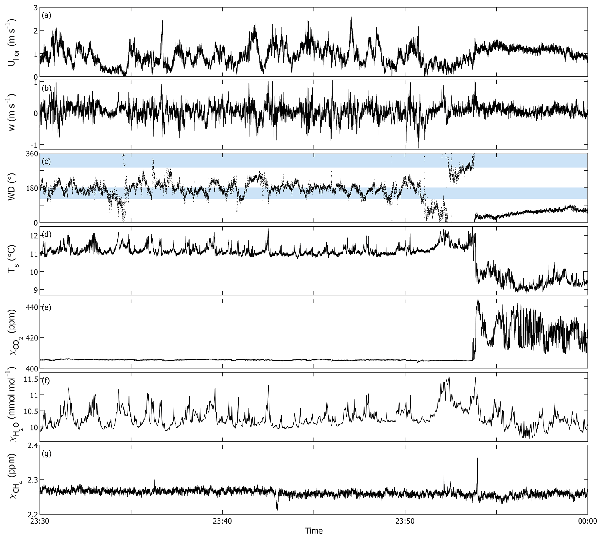
Figure A1 Example of a case with deviating wind direction on 7 August 2018 between 23:30 and 00:00 UTC. All data were measured at 10 Hz. (a) Horizontal wind speed. (b) Vertical wind speed. (c) Wind direction. The light-blue bars mark the accepted wind sectors. (d) Sonic temperature. (e) CO₂ dry mixing ratio. (f) H₂O mixing ratio. (g) CH₄ dry mixing ratio.

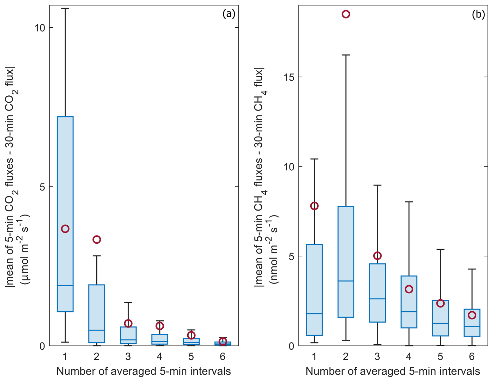
Figure A2 Absolute difference between the averaged 5 and 30 min fluxes for CO₂ (a) and CH₄ (b) as a function of the number of averaged 5 min intervals. The boxes indicate the upper and lower quartiles and the median. The whiskers are the maximum and minimum of non-outliers. The circles indicate means. Outliers are not shown.