Surface CO₂ gradients challenge conventional CO₂ emission quantification in lentic water bodies under calm conditions

Lakes are hotspots of inland carbon cycling and are important sources of greenhouse gases (GHGs) such as carbon dioxide (CO₂). The significant role of CO₂ in the global carbon cycle makes quantifying its emission from various ecosystems, including lakes and reservoirs, important for developing strategies to mitigate climate change. The thin boundary layer (TBL) method is a common approach to calculating CO₂ fluxes from CO₂ measurements in both water and air, as well as wind speed. However, one assumption for the TBL method is a homogeneous CO₂ concentration between the measurement depth and the water surface where gas exchange takes place. This assumption might not be true under calm conditions, when microstratification below the surface slows the vertical exchange of gases. We used a floating outdoor laboratory to monitor CO₂ concentrations at 5 and 25 cm depth, CO₂ concentration in the air, wind speed, and water temperature profiles for 1 week in the Bautzen Reservoir, Germany. While we found homogeneous CO₂ concentrations in the two depths at wind speeds above 3 m s⁻¹, there was a vertical gradient observed during windless nights. The concentrations observed temporally ranged from undersaturation to supersaturation at 25 and 5 cm, respectively. Fluxes calculated from the measured concentrations therefore would change from negative to positive, depending on the measurement depth. Simultaneous eddy covariance (EC) measurements showed that even the measurements close to the surface underestimated the actual CO₂ concentration. Oxygen measurements support our hypothesis that plankton respiration at the water surface causes a periodic CO₂ concentration gradient from the surface to the underlying water. Until now, the depth of CO₂ measurements has not been questioned, as long as measurements were done in the upper mixed layer and close to the surface. Our results provide evidence that representative measurements of CO₂ in the water strongly depend on depth and time of measurements.

1 Introduction

Lakes are hotspots of inland carbon cycling and are important sources of greenhouse gases (GHGs), such as carbon dioxide (CO₂). The significant role of CO₂ in global warming and climate dynamics makes quantifying its emission from various ecosystems, including lakes and reservoirs, important for developing strategies to combat climate change. Proper measurement of CO₂ emissions from lakes is the basis for robust global CO₂ emission quantification (Raymond et al., 2013; Lauerwald et al., 2023).

Eddy covariance (EC) is one of the most advanced methods used to quantify GHG fluxes between water and atmosphere, as it provides direct measurements covering large footprint areas at high temporal resolution (Aubinet et al., 2012). However, EC systems require a large homogeneous surface area to ensure accurate flux measurements. It is also limited by its costs and requirements for maintenance. Thus, there is a restricted number of EC sites on lakes worldwide (Golub et al., 2023). EC measures the total gas flux between the water and atmosphere, including diffusion and ebullition. However, in contrast to methane, which is often emitted by gas bubbles, CO₂ fluxes at the water surface are nearly exclusively driven by diffusion. The by far most used approach to quantify diffusive aquatic GHG fluxes is the thin boundary layer approach (TBL, Lauerwald et al., 2023), also referred to as the flux gradient method. The TBL approach, in contrast to EC, is an indirect measurement used to quantify diffusive gas exchange across the water–atmosphere interface. The TBL flux is derived from the concentration gradient between the water ($c_{{\mathrm{CO}}_{\mathrm{2}}\mathrm{water}}$) and the theoretical concentration at equilibrium with the air ($c_{{\mathrm{CO}}_{\mathrm{2}}\mathrm{equilibrium}}$), multiplied by the gas exchange velocity (k, Eq. 1).

$$\begin{array}{}\text{(1)}& F_{{\mathrm{CO}}_{\mathrm{2}}}=k\cdot \left(c_{{\mathrm{CO}}_{\mathrm{2}}\mathrm{water}}-c_{{\mathrm{CO}}_{\mathrm{2}}\mathrm{equilibrium}}\right)\end{array}$$

This method is much simpler than EC because it only requires concentration measurements in both the water and the atmosphere. The gas exchange velocity can be estimated from meteorological data, typically wind speed and potentially temperature or fetch, using empirical models (Cole and Caraco, 1998; McGillis et al., 2004; MacIntyre et al., 2010; Vachon and Prairie, 2013; MacIntyre et al., 2021). The temporal resolution can be comparable to the EC method when using submerged CO₂ probes. However, for both methods, uncertainties arise from situations involving very low wind speeds.

When there is no wind, EC systems cannot measure at all because the method relies on air movements (Aubinet et al., 2012; Podgrajsek et al., 2014). Additionally, the TBL approach encounters difficulties under windless conditions. While wind is the primary driver of gas transfer velocity and surface turbulence in large water bodies, its influence decreases under calm conditions, where factors such as the mixed layer depth (Rutgersson et al., 2008), surface cooling-induced convection (MacIntyre et al., 2010; Heiskanen et al., 2014; Andersson et al., 2017; MacIntyre et al., 2010), and the lake's morphometry (Schilder et al., 2013) gain prominence in controlling gas exchange velocities. For example, Podgrajsek et al. (2015) showed that high CO₂ fluxes in calm conditions can be explained by convective cooling. Further, most parametrizations of k rely heavily on wind speed and assume a zero intercept, leading to significant uncertainties under calm conditions. While factors like turbulence and convection are often considered in the context of their influence on k only, they also play a critical role in near-surface CO₂ gradients. This may lead to systematic underestimation of k under windless conditions. Although studies to improve k models exist (Cole et al., 2010; Crusius and Wanninkhof, 2003; MacIntyre et al., 2010; Vachon and Prairie, 2013), to our knowledge, the effect of uncertainty in $c_{{\mathrm{CO}}_{\mathrm{2}}\mathrm{Water}}$ measurements on the TBL approach has received little attention.

In calm conditions, the absence of wind significantly reduces turbulence, leading to surface microstratification. This microstratification creates distinct layers within the mixed layer, each with varying temperatures and solute concentrations, including CO₂ (Åberg et al., 2010). Specifically, microstratification may result in dissolved gas gradients near the water's surface, suggesting that the actual layer engaging in atmospheric exchange becomes very thin. This challenges the assumption of the TBL approach that water just below the surface accurately represents the layer of gas exchange.

The critical layer of diffusive gas exchange is the surface microlayer (SML). The SML is the interface between the water and the atmosphere and is characterized by high biological activity and physical processes that affect the interaction with the atmosphere (Gladyshev, 2002; Wurl et al., 2011). The SML is known for its enriched concentrations of phytoplankton, organic and inorganic solutes, and particles (Hardy, 1982). These components define the SML as a distinct layer situated between the atmosphere and the underlying water. In the ocean, surfactants in the SML were found to reduce the diffusive gas exchange with the atmosphere by 32 % (Pereira et al., 2018). Mustaffa et al. (2020) found a reduction in fluxes of 62 % in the presence of natural slicks. Under calm conditions, the SML thickens, becoming even more crucial for the diffusive exchange of gases (Rahlff et al., 2017). However, despite its importance, there remains a gap in our understanding of the interactions between the atmosphere, the SML, and the water beneath, particularly in freshwater environments.

Dynamics in gas exchange between the epilimnion, the surface layer, and the atmosphere could lead to systematic uncertainty in the quantification of the surface gas concentration, as samples might be collected from depths that do not accurately reflect the conditions of the water–atmosphere interface. In a recent study, Rudberg et al. (2024) explored how spatial and temporal differences affect the influence of k and $c_{{\mathrm{CO}}_{\mathrm{2}}}$ on the variability in $F_{{\mathrm{CO}}_{\mathrm{2}}}$. By deploying a floating chamber over several hours, the gas concentration in the chamber was equilibrated with the gas concentration in the surface water and enabled the quantification of the surface CO₂ concentration. With this approach they demonstrated that over periods of 1–9 d, $c_{{\mathrm{CO}}_{\mathrm{2}}}$ contributed more to $F_{{\mathrm{CO}}_{\mathrm{2}}}$ variability than k. This finding emphasizes the need for precise $c_{{\mathrm{CO}}_{\mathrm{2}}}$ measurements when estimating fluxes using models. Similar research has been conducted in the ocean. Although CO₂ samples for gradient-based flux models are usually collected a few meters below the water surface, Calleja et al. (2013) found significant gradients between depths of 5–8 m. Hari et al. (2008) found different CO₂ concentrations at 0.1 and 0.5 m depth while investigating a new method for CO₂ measurements. However, while these differences are attributed to varied biological activities in the different depths, there is a lack of knowledge about the formation and characteristics of such gradients, especially with regard to the SML and diffusive gas exchange with the atmosphere.

To better understand the importance of vertical CO₂ gradients at the water–atmosphere interface, we conducted an extensive field experiment in a eutrophic reservoir. Our study is based on two key hypotheses.

1. Temporal gradients of CO₂ concentrations are present close to the water surface.

2. These gradients are influenced by meteorological factors, such as wind.

To assess the effect of a potential surface CO₂ gradient on CO₂ fluxes, we compared fluxes calculated by the TBL approach with fluxes measured by EC during the same period.

2 Materials and methods

2.1 Study site

Our study site, Bautzen Reservoir in Germany (51.218° N, 14.466° E), is a dimictic reservoir. High wind exposure, a relatively large surface area (533 ha), circular shape, and the shallow depth (mean 7.4 m, maximum 13.5 m) result in weak stratification during summer in some years (Benndorf, 1995; Spank et al., 2023). The eutrophic to hypereutrophic reservoir (Kerimoglu and Rinke, 2013) serves to regulate the flow of the Spree River – the main river of Berlin. A preceding study showed CO₂ uptake of −9.8 and −71.0 g C m⁻² during the ice-free seasons of 2018 and 2019, and CH₄ fluxes of 24.0 and 23.2 g C m⁻², respectively (Spank et al., 2023).

2.2 Meteorological field observatory

A floating outdoor laboratory was operated to continuously observe the mass and energy exchange between the water surface and the atmosphere. A detailed description of the floating outdoor laboratory and its instrumentation can be found in Spank et al. (2020, 2023, 2024). The floating outdoor laboratory provided reference data of the carbon dioxide flux ($F_{{\mathrm{CO}}_{\mathrm{2}}}$) between the water surface and the atmosphere, as well as data of wind speed (U), air temperature (T_a), relative air humidity (RH), air pressure (p_a), solar radiation (R_g), and water temperature (T_w) at a temporal resolution of 30 min. In addition, the floating outdoor laboratory served as a carrier for the devices used during the measurement campaigns. The measurement height of meteorological sensors was 2 m above the water surface in accordance with international standards. Water temperature (T_w) was measured at depths of 0.25, 0.50, 0.75, 1.0, 1.5, 2.0, 2.5, 3.0, 4.0, 5.0, 6.0, 8.0, 10.0, 12.5, and 15.0 m. The eddy-covariance-measuring system, which provides $F_{{\mathrm{CO}}_{\mathrm{2}}}$, was instrumented according to standards and guidelines given by Lee et al. (2004), Foken and Mauder (2024), Aubinet et al. (2012), and Burba (2013). EC post-processing was based on the methodologies of Carbo Europe (Aubinet et al., 1999) and ICOS (Sabbatini et al., 2018), utilizing the software EddyPro 7.0.8 (LI-COR Biosciences 2023). The special site conditions and the platform movement were taken into account and addressed by a correction of the sensor misalignment beforehand (Spank et al., 2020, 2023). The EC data are representative of the pelagic zone of the Bautzen Reservoir. In particular, a footprint analyses proved that effects and disturbances from surrounding terrestrial sites can almost completely be ruled out (Spank et al., 2023). The correctness and quality of data were checked using the methodology of Foken and Wichura (1996). Quality features, i.e., stationarity and turbulence characteristics, were computed for the individual 30 min data records and classified according to the nine-step classification scheme of Mauder et al. (2006), where 1 is best and 9 is worst. Only 30 min data records that fulfilled criteria for quality levels 1–6 were considered. In addition, the random sampling error was calculated according to Finkelstein and Sims (2001) and was used to capture the non-systematic uncertainty in $F_{{\mathrm{CO}}_{\mathrm{2}}}$ and $F_{{\mathrm{CH}}_{\mathrm{4}}}$. Further information on the uncertainty analysis and the analysis of systematic measurement uncertainties in the EC data can be found in Spank et al. (2025). While this study focuses on low wind situations where EC measurements can potentially be biased due to a lack of turbulence and gustiness, no such issues were observed during the investigated period. Conversely, all flux data exhibited sufficient turbulence and stationarity. This observation was also confirmed by spectral analyses, which showed clearly developed power and cospectra.

2.3 Dissolved gases

To detect potentially occurring dissolved CO₂ concentration gradients at the water surface, we deployed two CO₂ probes (CONTROS HydroC^® CO₂, -4H- JENA engineering GmbH, Kiel, Germany) at different depth from 18 to 25 September 2022 (hereinafter referred to as the study period). These probes, featuring diffusive membranes with a diameter of 8 cm, were positioned so that the central points of their membranes were situated at depths of 0.05 and 0.25 m, respectively. We used a frame that consisted of two aluminum bars that were connected by two cross bars in the middle. Aluminum extensions on the cross bars were used to mount the CO₂ probes horizontally and allow adjustment of the measurement depth. Buoyancy floats in the four corners were used to make the frame float below the surface (Fig. S1). The CO₂ probes were operated at 24 VDC, provided by the floating platform. To maintain the integrity of surface water stratification, we left the membranes of the CO₂ probes uncovered. CO₂ was measured every 1 min, and data were internally logged by the probes. The probes performed internal zero baseline corrections once a day.

CO₂ probe performance was validated before deployment. After deployment, internal data required post-processing (as described in Fietzek et al., 2014) because the measurements were out of the factory calibration range. In brief, the internal zero measurements using CO₂ absorbents generate frequent calibration points for pCO₂=0. Daily zero measurements were used to calibrate signal outputs between the last and the next zero measurements. Finally, a modified polynomial function was used to determine the corrected CO₂ concentrations (Supplement S1). The equilibrium concentration for CO₂ was derived from the EC CO₂ analyzer (LI-7200, LI-COR Environmental, Inc., Lincoln, NE, USA). Oxygen concentrations were measured every 15 min by optical O₂ loggers. Surface O₂ concentration at 0.05 m depth was measured with a miniDOT logger equipped with a miniWIPER (Precision Measurement Engineering, USA; wiping frequency 12 h) mounted at the same depth as the surface CO₂ probe. A D-Opto oxygen logger (ZebraTech, Nelson, NZ) was installed in the bottom water at 1 m above the sediment using a separate mooring. Both oxygen sensors were calibrated using a two-point calibration at 0 % and 100 % oxygen saturation and corrected for potential drift.

2.4 Data and statistical analysis

The platform data were prepared and exported in Python. For this study, the platform data, CO₂ probe data, and oxygen data were compiled in R (R version 4.4.1, R Core Team, 2024). All subsequent analyses, statistical computations, and visualizations were performed in R (Supplement S2). CO₂ and oxygen measurements were averaged over 30 min periods. Gas fluxes were calculated from in situ water and air pCO₂ and k (calculated from U₁₀ after Cole and Caraco, 1998) using Eq. (1).

3 Results

In 2022, the Bautzen Reservoir was thermally stratified starting in the beginning of May. During the stratified period (mean mixed layer depth = 4.4 m), the maximum T_w at the surface was 30 °C, while T_w above the ground reached a maximum of 13 °C (Fig. A1). On 9 September 2022, a thunderstorm with strong winds hit the Bautzen region, leading to a shutdown and subsequent 5 d outage of the measurement platform. This storm also marked the end of the stratified season and the beginning of the mixing of the reservoir. On 18 September, which marks the beginning of our extensive GHG measurements, T_w was 16 °C at both the surface and bottom. The oxygen concentration was 9.1 mg L⁻¹ at both the surface and the bottom.

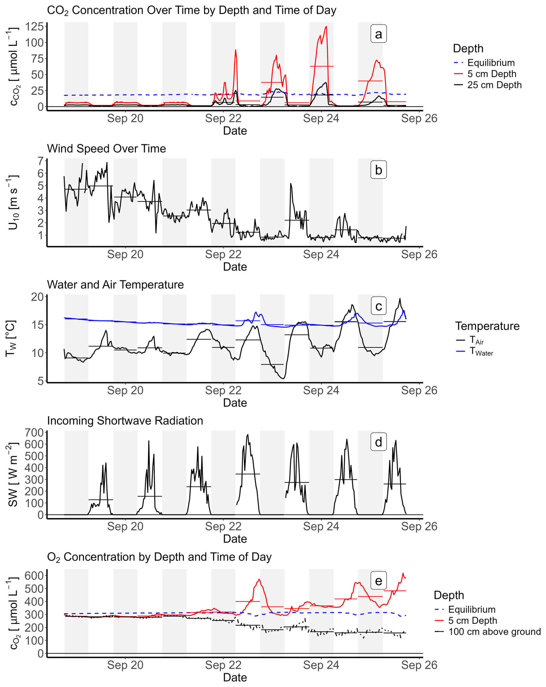
Figure 1 CO₂ concentrations (a) measured at 0.05 and 0.25 m depth (red and black line, respectively) and equilibrium concentration with the atmosphere (dashed blue line). Wind speed at 10 m height (U₁₀, b), water temperature at 0.25 m depth + air temperature (c), and incoming shortwave radiation (SW, d). Oxygen concentrations (e) at 0.05 m depth and at 1 m above ground (red and black line, respectively), as well as equilibrium concentration with the atmosphere (dashed blue line). In all plots, horizontal bars show mean values of days and nights and gray shading indicates nighttime.

Our measurement period can be divided into two parts with differing weather conditions. The first period, from 19 to 21 September, was windy with U₁₀ mostly above 3 m s⁻¹. In contrast, during the second half of our sampling period, wind speeds were mostly below 3 m s⁻¹, with 63 % of these times even falling below 1 m s⁻¹ (Fig. 1b).

The CO₂ concentrations near the water surface showed a fundamentally different behavior during these two periods (Fig. 1a). During the windy period, CO₂ was permanently undersaturated and just above zero. In contrast, high CO₂ concentrations up to 125 µmol L⁻¹ were observed during the calm period. Notably, nightly CO₂ concentrations at both depths were 10 to 20 times higher during the calm period compared to the windy period. Starting on 22 September, nightly CO₂ concentrations exceeded the equilibration concentration, leading to temporary supersaturation in calm nights. While the nightly mean CO₂ concentration at 5 cm depth exceeded the equilibration concentration in the nights of 23 to 26 September, the mean concentration at 25 cm depth never surpassed equilibrium. The CO₂ concentration at the water surface showed a consistent diurnal pattern during the entire study period. At night, the CO₂ concentration at 5 cm depth was generally higher than at 25 cm depth. Thus, a gradient of CO₂ concentration near the water surface developed every night of our study period. In contrast, no such gradient was observed during the day. At both depths, CO₂ concentrations increased with the disappearance of shortwave radiation at sunset and decreased after sunrise again (Fig. 2d).

The oxygen concentration patterns also differed between the two periods. During the windy period, O₂ concentrations at both 5 cm depth and at the bottom were slightly undersaturated. When the water column started stratifying again (Fig. 1e), O₂ concentrations at the two depths started to diverge. The O₂ concentration at the bottom continuously decreased over the rest of the sampling period. The concentration at 5 cm increased to supersaturation, showing clear diurnal patterns of oxygen production and consumption (Fig. 1e).

Mean air temperatures (T_a) ranged between 9 and 15 °C, with distinct diurnal patterns. The water temperature at 25 cm depth (T_w25) decreased slightly from 16 to 15 °C during the measurement period, except on 23, 24, and 25 September, when T_w25 increased by 1 °C during the day (Fig. 1c). During the days of 23, 24, and 25 September, T_a was higher than the water temperature. On all other days and nights, T_w25 consistently remained higher than the air temperature.

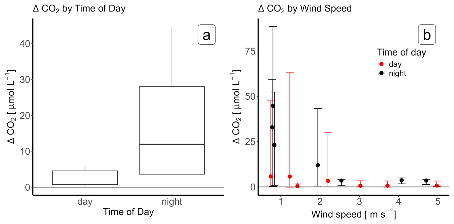
Figure 2 Dependence of the absolute difference in CO₂ concentration between 5 and 25 cm depth on the diurnal period (a), expressed as ΔCO₂ in µmol L⁻¹. Panel (b) shows the relationship between ΔCO₂ and wind speed (U₁₀), with daytime observations highlighted in red and nighttime observations in black. Whiskers show minima and maxima of the respective period.

To gain a more detailed understanding of the CO₂ gradients at the surface, we calculated the difference in CO₂ concentrations between 5 and 25 cm depths (ΔCO₂). The mean concentration gradient was significantly steeper during the night compared to during the day (t test, p<0.05, Fig. 2a). The magnitude of ΔCO₂ depended on wind speed (Fig. 2a). Generally, the mean CO₂ gradient was lower at high wind speeds for both day and night. However, while low wind speeds did not lead to higher CO₂ gradients during the day, the gradients in calm nights were 5- to almost 10-fold steeper (Fig. 2b). This diurnal development of a CO₂ gradient at the surface should have affected CO₂ emissions.

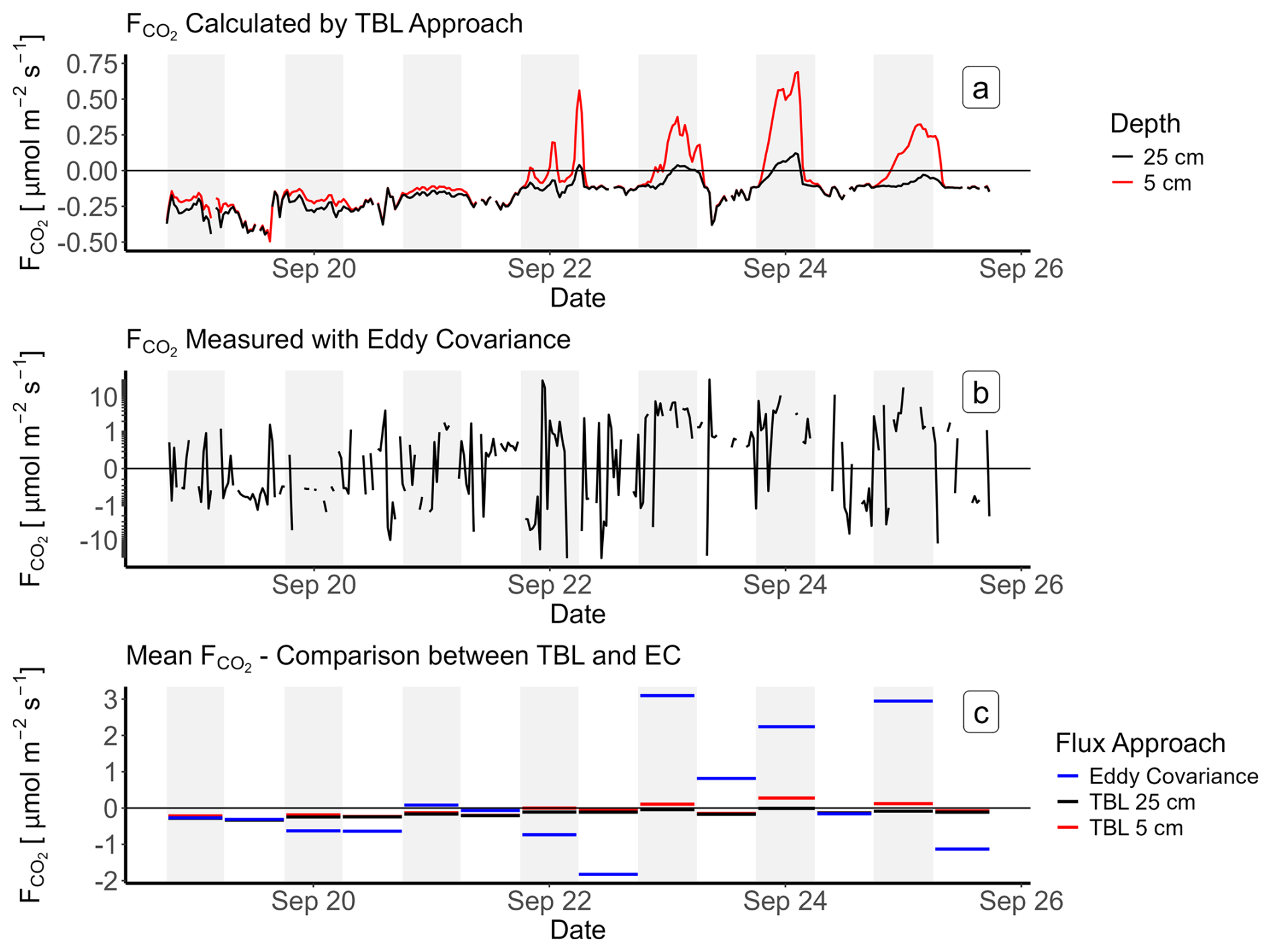
Figure 3 Comparison of fluxes ($F_{{\mathrm{CO}}_{\mathrm{2}}}$) derived from eddy covariance (EC) measurements and the thin boundary layer (TBL) approach. TBL fluxes (a) derived from $c_{{\mathrm{CO}}_{\mathrm{2}}\mathrm{\_}\mathrm{0.05}}$ and $c_{{\mathrm{CO}}_{\mathrm{2}}\mathrm{\_}\mathrm{0.25}}$ are shown as red and black lines, respectively. $F_{{\mathrm{CO}}_{\mathrm{2}}}$ measured by EC (b) is shown as black lines. $F_{{\mathrm{CO}}_{\mathrm{2}}}$ averaged over every day and night period is shown in panel (c), where red bars are fluxes derived from $c_{{\mathrm{CO}}_{\mathrm{2}}\mathrm{\_}\mathrm{0.05}}$, black bars derived from $c_{{\mathrm{CO}}_{\mathrm{2}}\mathrm{\_}\mathrm{0.25}}$, and blue bars derived from EC measurements. All fluxes are shown in units of µmol m⁻² s⁻¹. Gray shading shows nighttime in all subplots.

We used our CO₂ concentration data to calculate $F_{{\mathrm{CO}}_{\mathrm{2}}}$ with the TBL approach and compared these fluxes with measurements done with eddy covariance (Fig. 3). During the windy period, TBL fluxes were negative regardless of which CO₂ probe data we used and comparable to the fluxes measured by EC (Fig. 3a, b, and c). On calm nights, supersaturation of CO₂ led to positive TBL fluxes with data from both depths. Because at 25 cm depth oversaturation was only reached at the end of the night, mean night fluxes derived from 25 cm depth remained negative (Fig. 3c). EC fluxes during these nights were positive too but significantly higher than TBL fluxes (Fig. 3b, c). In 5 out of the 14 cases, the flux direction differed between the TBL approach and EC measurements when using the measurements of the 25 cm probe for the TBL approach. In contrast, when using CO₂ measurements from the 5 cm probe, only 2 out of 14 instances show different flux directions. During our study period of 7 d, the total CO₂ emissions were −2.2 g m⁻² when calculated using the 5 cm data, −4.2 g m⁻² based on 25 cm data, and 4.6 g m² as recorded by the eddy covariance system.

4 Discussion

Our data revealed how changes from windy to calm weather and from a mixed water column to stratification within 1 week influenced microstratification and its effect on greenhouse gas exchange between the lake and the atmosphere. Our detailed CO₂ concentration measurements clearly showed the temporal development of CO₂ gradients at the water surface. This observation is consistent with previous studies like Hari et al. (2008), whose results indicate CO₂ gradients within the upper 50 cm of the water layer.

During the windy period, CO₂ concentrations were almost zero at daytime, probably caused by photosynthetic CO₂ consumption by abundant phytoplankton. CO₂ undersaturation in highly productive lakes is a common observation (Balmer and Downing, 2011; Zagarese et al., 2021). In this period, CO₂ concentrations were consistently lower than the atmospheric equilibrium concentration, turning the reservoir into a CO₂ sink during this time. The temperature profiles and the oxygen concentrations measured at the surface and above the bottom suggest that the entire water column was mixed in that period. This also likely leads to a homogeneous vertical distribution of CO₂. The fact that there was no thermal stratification in this time means that the phytoplankton's CO₂ uptake stripped CO₂ from the entire water column rather than only from the smaller volume of the upper mixed layer. Consequently, more CO₂ would be required to increase the concentration at the surface compared to a stratification scenario. This observation is supported by the fact that no CO₂ gradient was measured during the day, while a slight gradient was detected at night. This occurs because CO₂ is consumed quickly during daylight hours, whereas at night, the uptake of CO₂ from the atmosphere leads to slightly higher concentrations at the water surface. This was reflected by our 5 cm probe measuring concentrations closer to atmospheric equilibrium than the 25 cm probe.

When the wind ceased at 21 September, the vertical distribution of gas concentrations changed. Starting on this day, oxygen concentrations at the surface and at the bottom began to increase and decrease, respectively. This observation indicates that the reservoir slowly underwent stratification again. Because the mixing depth was much greater during the windy period compared to the calm period, the water volume available to dissolve CO₂ was also much greater. Consequently, the lower wind speed in the second half of the week decreased both the mixing depth and the available volume. During these calmer nights, respiration in the shallow mixed layer led to significant CO₂ accumulation at the surface. Additionally, microstratification within the top 25 cm of the water column could further restrict the volume available for CO₂ accumulation, potentially leading to even higher concentrations (Fig. 4). While there was no difference in CO₂ gradients during calm daylight hours compared to windy days, we observed notably high CO₂ concentrations within the top 25 cm during calm nights. Our findings are consistent with a study of Åberg et al. (2010), who found that short-term CO₂ variations at the surface were best linked to thermal dynamics within the upper mixed layer, whereas parameters like wind and radiation did not influence CO₂ concentrations. In our study we found a negative effect of incoming solar radiation on CO₂ concentrations during the day but positive feedback during the night. Further, varying CO₂ concentrations have been previously linked to changes in lake metabolism after storms (Vachon and del Giorgio, 2014).

Interestingly, the 5 cm probe, despite being closer to the surface, recorded higher CO₂ concentrations than in the underlying water. This requires a CO₂-producing process in the surface layer, likely respiration. There are various groups of organisms that could increase CO₂ in the 5 cm layer, such as neuston, which comprises organisms living at or even within the surface micro layer. Phytoplankton was found to float at the water surface at wind speeds lower than 3 m s⁻¹ (Zhang et al., 2021). Further, some species migrate from the lower boundary of the epilimnion to the surface during night. This behavior is called diel vertical migration and is used to access food while avoiding predators that need light for hunting (Ringelberg, 1999). Both neuston and migrating species respirate during the night, thereby producing CO₂. Furthermore, the vertical mixing during windy periods likely increased nutrient availability for phytoplankton, potentially triggering growth and accumulation of phytoplankton at the water surface (Nürnberg et al., 2003). The phytoplankton switches from net photosynthesis during the day to net respiration at night, thereby increasing CO₂ concentration at night. In the calm period, mean gross primary production and respiration as calculated from oxygen data were 10.4 and −9.0 mg O₂ L⁻¹ d⁻¹, respectively, which are comparable to other hyper-eutrophic lakes, especially after storm events (Williamson et al., 2021). During algal blooms, the water surface is often covered by a mat of floating phytoplankton. Although we lack chlorophyll data, satellite images taken before and after our measurement period suggest rapid algal growth following the storm events that occurred just before our study (Fig. B1). Such mats can become very dense, possibly increasing CO₂ production and accumulation even more.

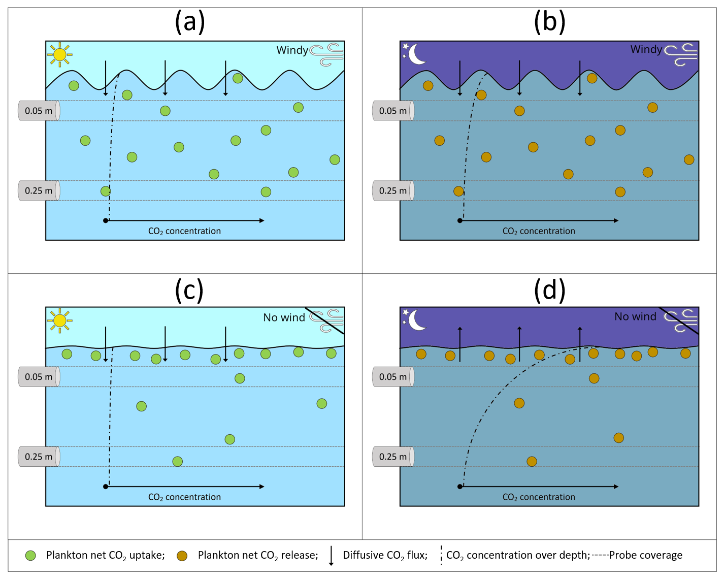
Figure 4 Schematic of CO₂ accumulation in the surface water, with CO₂ probes located at 5 and 25 cm depth. (a) Wind-induced turbulence causes homogeneous distribution of plankton, resulting in CO₂ decrease in both measuring depths during the day. (b) Wind-induced turbulence causes homogeneous distribution of plankton. CO₂ is produced by respiration, but the CO₂ concentration across the whole water column is low, thus respiration compensates for strong undersaturation. CO₂ uptake from the atmosphere causes slightly increased concentration at 5 cm. (c) CO₂ concentration is low over the whole mixed layer, but calm conditions cause plankton to accumulate at the surface. (d) Calm conditions cause plankton to accumulate at the water surface. Respiration causes a CO₂ increase in this layer, which causes CO₂ emissions during calm nights.

Besides biologic activity, convective mixing within the top water layer can play an important role in the distribution of CO₂ concentrations. Convective mixing, driven by water density differences due to cooling at the water surface, can enhance the vertical movement of water, thereby influencing the distribution of CO₂ in the water column. While we did not find signs of thermal microstratification at the surface during nights with strong CO₂ gradients, we contrastingly observed conditions favoring convection (Fig. 1c). Further, meteorological parameters, such as atmospheric stability, emitted longwave radiation, and sensible heat flux, indicate unstable conditions in the air above the water. From this, we infer that the biomass accumulated at the water surface could produces CO₂ at rates that exceed its transport in the upper water layer or that the algal mats acted as a physical barrier between the water and air, leading to increased stability of the water beneath the mats, which reduces the influence of atmospheric instability on the water below. In our case the high CO₂ concentrations at the surface were not driven by convective upward mixing of CO₂ rich water but by biological activity at the surface.

The CO₂ gradient measured during calm nights fundamentally influenced the fluxes calculated with the TBL method. Fluxes derived from concentrations at 0.05 m depth were closer to the fluxes measured by EC than fluxes derived at 0.25 m depth. However, TBL fluxes derived from 0.05 m were a magnitude lower than those of EC. This could be due to either an unprecise parametrization of k or inaccurate CO₂ measurement. Many previous studies showed that water-side convection has a significant contribution to the gas transfer coefficient under calm conditions (Eugster et al., 2003; Rutgersson and Smedman, 2010; Heiskanen et al., 2014; Podgrajsek et al., 2015). However, these studies reported increased fluxes up to 200 %, which would still underestimate TBL fluxes in our experiment, compared to EC fluxes.

While it is generally acknowledged that daytime measurements do not reflect the concentrations at night (Erkkilä et al., 2018), the depth of CO₂ measurements has not been questioned so far, as long as measurements were done in the upper mixed layer and close to the surface. Our measurements provide evidence that representative measurements of the CO₂ concentration in the water strongly depend on depth and time of measurements. In our results, the depth of measurement even determined whether the TBL method would result in efflux or influx (Fig. 3b). This was especially visible at night, when the flux calculated from the CO₂ concentration measured at 25 cm depth was negative, while both EC measurements and TBL based on the measurements at 5 cm showed significant positive fluxes. The fact that the EC fluxes were higher than the TBL fluxes based on the 5 cm probe could be explained by the CO₂ gradient which probably continued towards the water–atmosphere interface.

Our uppermost probe measured the mean CO₂ concentration between 1 and 10 cm depth, and it is plausible that the concentration at the water surface was even higher than measured by the probe. Based on our results, the highest CO₂ concentration is expected to occur at the very surface of the water, driven by nighttime respiration and restricted mixing. However, current measurement methods are not able to resolve such small-scale vertical gradients within the SML. While floating chambers have been used to measure CO₂ in the surface by deploying them as closed systems, therefore equilibrating the chamber volume with the surface water, this method is limited by slow equilibration times and insufficient temporal resolution (Rudberg et al., 2021). Therefore, advanced measurement techniques with higher vertical and temporal resolution are necessary to accurately capture steep CO₂ gradients and to understand the dynamics of CO₂ exchange at the water–atmosphere interface.

5 Conclusions

We showed that, under the right conditions, a significant gradient of CO₂ concentrations at a lake's surface can develop. This gradient was largest on windless nights. The gradient occurred at the same time as a phytoplankton bloom, from which we conclude that phytoplankton is the controlling source of CO₂. A thin surface layer with high CO₂ concentrations can develop only when limited mixing of the surface layer comes together with high accumulation of biomass in the surface water. This effect can be large enough to turn a CO₂ under-saturated lake into a temporary CO₂ source. This result partly explains the discrepancies of previous studies where high CO₂ fluxes measured by eddy covariance could not be found with the thin boundary layer method (Spank et al., 2020). We also show that uncertainty in the TBL method under calm conditions not only results from an incorrect parameterization of the gas transfer velocity but also from error-prone measurements of CO₂ in the water. Our findings imply that CO₂ emissions from eutrophic waters might be higher than previously thought – especially under calm conditions.

Appendix A: Detailed water temperature graphs

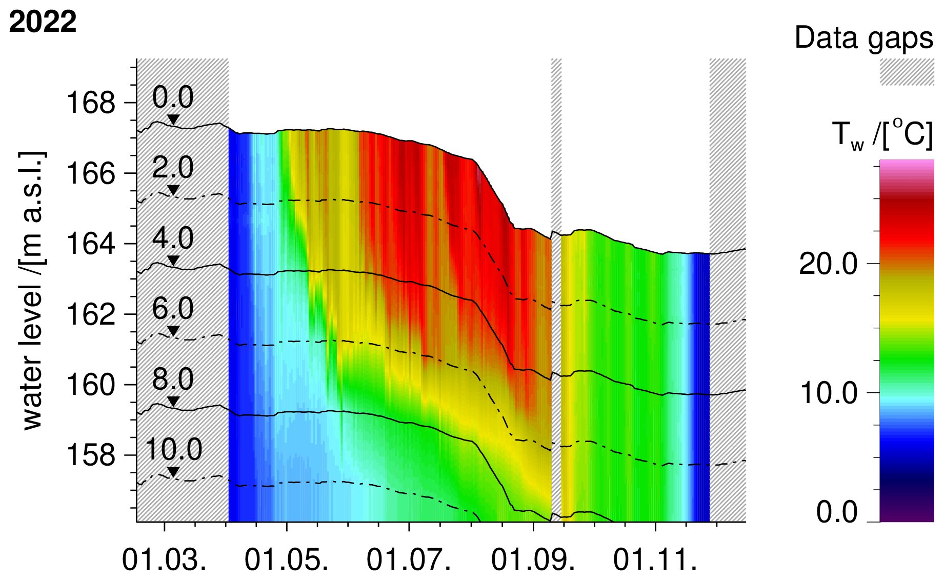
Figure A1 Water level (meters above sea level) and water temperature profile from 1 April to 28 November 2022 at the Bautzen Reservoir. Solid and dot-dashed black lines indicate water depths of 2, 4, 6, 8, and 10 m. Gray bars highlight missing data.

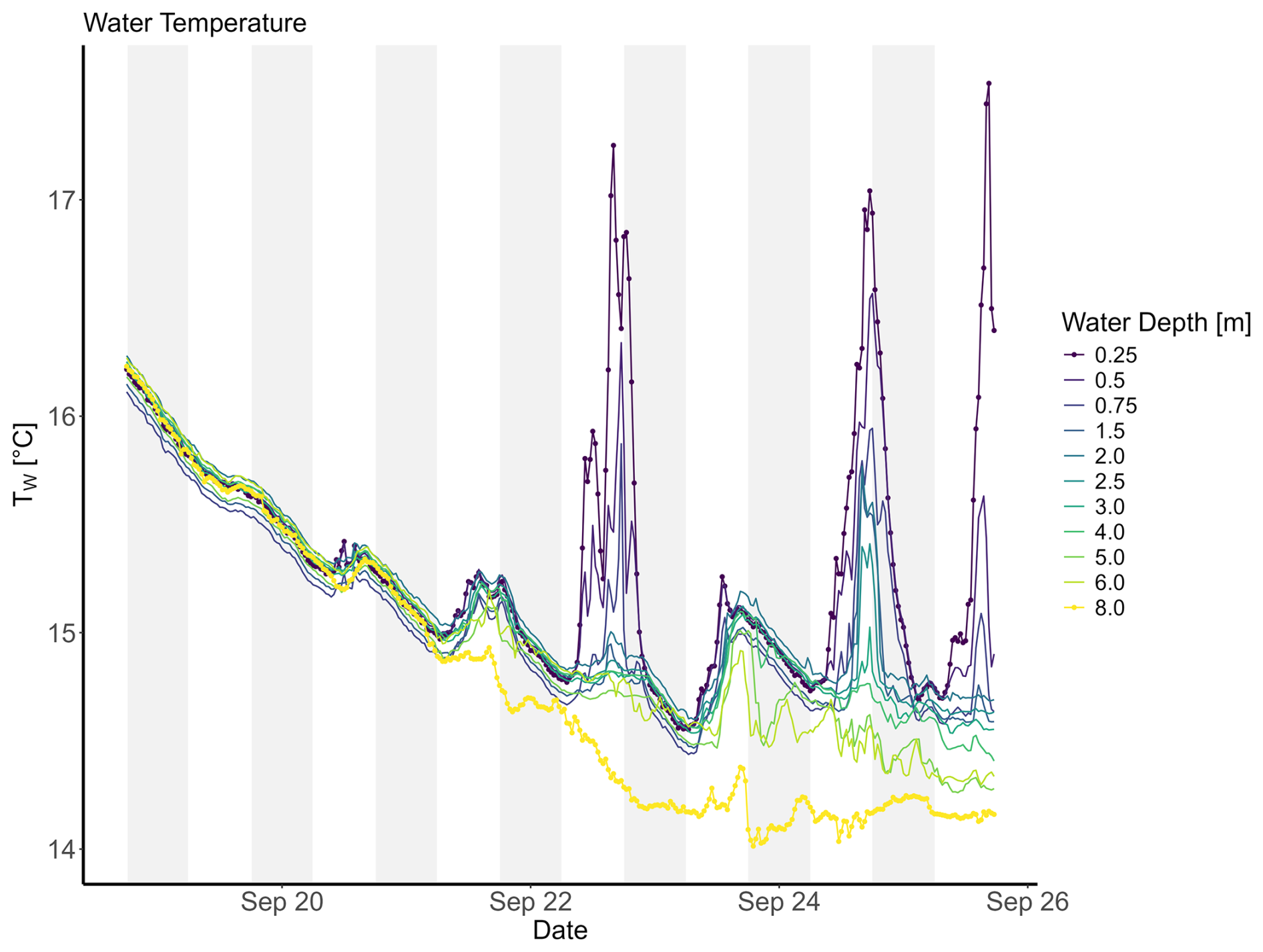
Figure A2 Detailed water temperatures across the water column during the extensive sampling period. Dotted dark purple and yellow lines highlight surface and bottom temperatures, respectively. Gray shading shows nighttime.

Appendix B: Satellite images of the reservoir

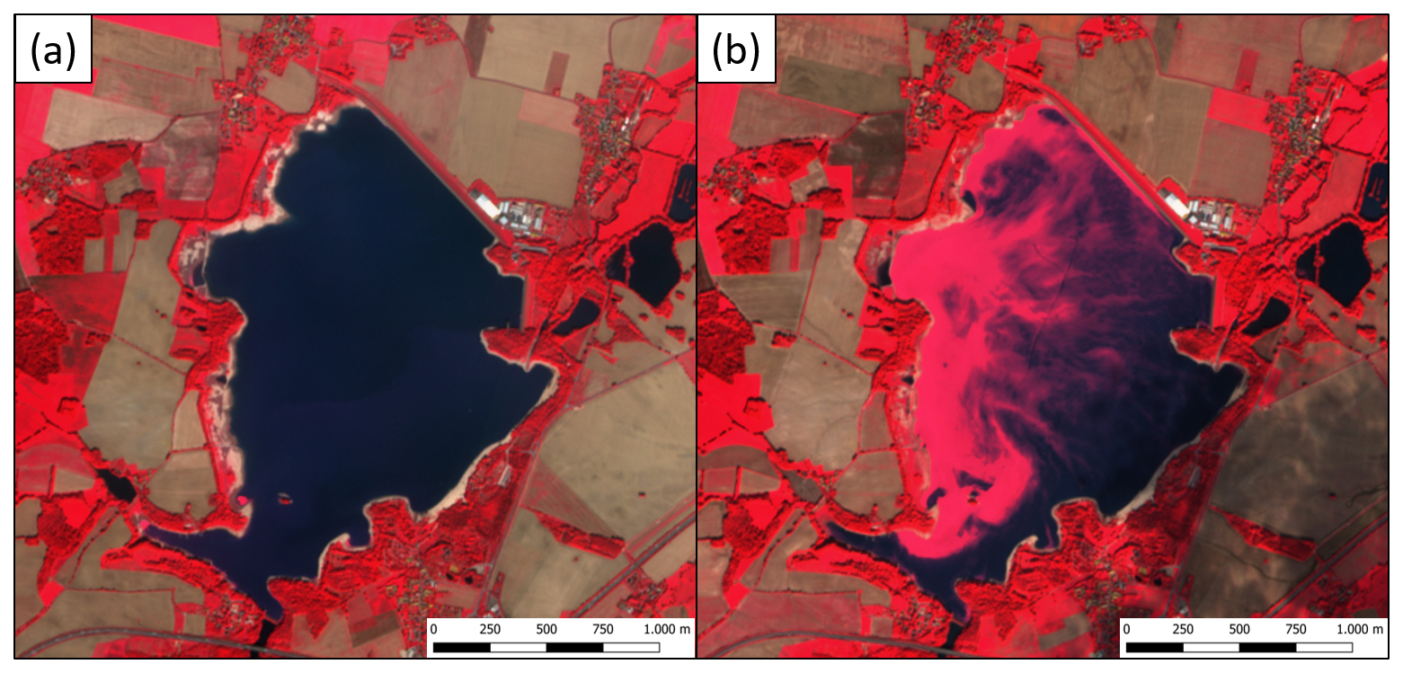
Figure B1 False color images from Sentinel-2 L2A taken on 5 September 2022 (a) and on 25 September 2022 (b) provided by the European Space Agency (ESA) and accessed via the EO Browser (https://apps.sentinel-hub.com/eo-browser/, last access: 8 August 2024, Sinergise Solutions d.o.o., a Planet Labs company). The date 5 September was selected because it was the last day without cloud coverage before the sampling period. The images show the state of the reservoir during the algal bloom described in this text. The false color images, which are typically used to highlight specific features like vegetation or water, do not show the water surface properly on 25 September, due to algal coverage. This clearly highlights the intensity of the algal bloom, which likely covered the water surface.