Intercomparison of biogenic CO₂ flux models in four urban parks in the city of Zurich

Quantifying the capacity and dynamics of urban carbon dioxide (CO₂) emissions and carbon sequestration is becoming increasingly relevant in the development of integrated monitoring systems for urban greenhouse gas (GHG) emissions. There are multiple challenges in achieving these goals, such as the partitioning of atmospheric measurements of CO₂ fluxes to anthropogenic and biospheric processes, the insufficient understanding of urban biospheric processes, and the applicability of existing biosphere models to urban systems. In this study, we applied four biosphere models of varying complexity – diFUME, JSBACH, SUEWS, VPRM – in four urban parks in the city of Zurich and evaluated their performance against in situ measurements collected over almost 2 years on park trees and lawns. In addition, we performed an uncertainty analysis of gross primary productivity (GPP), ecosystem respiration (R_eco), and net ecosystem exchange (NEE) of CO₂ based on the differences between the estimates of the four models and compared the estimated uncertainties and biospheric fluxes with the monthly anthropogenic CO₂ emissions of a wide urban area surrounding the four parks. The results showed that, despite the large differences in model architecture, there was considerable agreement in the seasonal and diurnal GPP, R_eco, and NEE estimates. Larger discrepancies between the four models were found for lawn GPP compared to tree GPP, while, for R_eco, the differences between lawns and tree areas were similar. On an annual scale, all models agreed, on average, that lawns acted as CO₂ sources and tree-covered areas as CO₂ sinks during the simulation period, with the exception of diFUME, which simulated both tree and lawn areas as CO₂ sources. diFUME and VPRM were more accurate in capturing the onset of the tree leaf growth in spring compared to JSBACH and SUEWS. On the other hand, JSBACH and SUEWS simulated soil water availability more accurately than the satellite-derived water index used by VPRM. The in situ observations revealed a very high spatial variability in lawn R_eco across the park areas. All models underestimated the lawn R_eco during spring in mowed, sunny locations, whereas the model simulations were closer to the observed R_eco in un-mowed, partially shaded locations. The mean monthly uncertainties in biogenic NEE reached 0.8 $\mathrm{\mu }\mathrm{mol}{\mathrm{m}}^{-\mathrm{2}}{\mathrm{s}}^{-\mathrm{1}}$, which is 10.2 % of the magnitude of the total CO₂ balance over the studied area during the month of June. This balance was composed of a mean anthropogenic flux of 8.7 $\mathrm{\mu }\mathrm{mol}{\mathrm{m}}^{-\mathrm{2}}{\mathrm{s}}^{-\mathrm{1}}$ and a mean biospheric flux of −0.5 $\mathrm{\mu }\mathrm{mol}{\mathrm{m}}^{-\mathrm{2}}{\mathrm{s}}^{-\mathrm{1}}$. Overall, this study highlights the importance of properly accounting for the biogenic CO₂ fluxes and their uncertainties in urban CO₂ balance studies, especially during the vegetation growing season, and shows that even simple models, such as VPRM, can adequately simulate the urban biospheric fluxes when appropriately parameterized.

1 Introduction

In the battle against the climate crisis, numerous cities have announced ambitious goals to achieve carbon neutrality in the coming decades. Their climate action plans include steps on reducing fossil fuel carbon dioxide (CO₂) emissions and increasing carbon removals by urban green areas. These plans have raised the need for observation-based monitoring of urban greenhouse gas (GHG) fluxes in order to follow the progress towards climate goals. However, the challenge lies in separating the CO₂ fluxes from anthropogenic emissions and biospheric emissions/uptake, as their signals are rapidly mixed in the atmosphere (Lauvaux et al., 2020). This is further complicated by the fact that both anthropogenic and biogenic CO₂ fluxes have distinct diurnal and seasonal cycles and respond to changes in the environment (Järvi et al., 2019; Stagakis et al., 2023b).

The net CO₂ balance or net ecosystem exchange (NEE) of biogenic CO₂ fluxes is the difference between ecosystem respiration (R_eco) and gross photosynthetic CO₂ uptake (or gross primary productivity, GPP). NEE is relatively small on an annual basis, especially in urban areas where a big fraction of the land is covered by built structures, but varies significantly on diurnal and seasonal scales (Stagakis et al., 2023a, b; Winbourne et al., 2022) and can significantly alter the atmospheric CO₂ observations. Recent studies have shown that urban NEE can offset between 0 % and over 100 % of the local anthropogenic CO₂ emissions depending on the area considered, the source/sink composition, the season, the day type, and the hour (Lauvaux et al., 2020; Stagakis et al., 2023a, b; Winbourne et al., 2022). A few studies used observations of isotopes and co-emitted species to discriminate between biogenic and anthropogenic CO₂ in the urban atmosphere (Pataki et al., 2003; Wu et al., 2022), but the estimates of biogenic CO₂ fluxes are associated with high relative uncertainties. Field observations, on the other hand, can provide very valuable information on urban biospheric processes but are hampered by the extreme heterogeneity of urban environments in terms of vegetation types and species, soil composition, management practices, and local meteorology, as well as by technical and logistical restrictions (Lal and Augustin, 2012). This creates a need to utilize models of biogenic CO₂ exchange to quantify and further partition the net flux from anthropogenic activities, e.g. via inversion methods (e.g. Lauvaux et al., 2020; Stagakis et al., 2023a).

In the past, numerous comprehensive models have focused on carbon exchange processes, including photosynthesis and soil and vegetation respiration at ecosystem level (Hari et al., 2017; Mäkelä et al., 2004; Zhao et al., 2016), but these models were primarily designed for forested or other natural ecosystems. It still remains a question how well they are able to represent carbon uptake processes in urban areas due to the very specific conditions, including high variability in soil and vegetation types and species, possible limitations in soil water availability, increased air pollutant loads, higher evaporative demand resulting from elevated temperatures and vapour pressure deficits, special light environments, and intensive management commonly taking place in urban green areas (Dahlhausen et al., 2018; Decina et al., 2016; Nielsen et al., 2007; Wohlfahrt et al., 2019). In recent years, different modelling approaches customized for urban areas have emerged with different strengths and weaknesses. Full carbon cycling/ecosystem models, such as JSBACH (Trémeau et al., 2024), can simulate in detail the processes behind carbon exchanges and carbon stocks. Their limitation lies in the fact that, within urban built environments, the soil is often disturbed and the soil carbon pool is rarely in equilibrium with the existing vegetation. As a result, the standard initialization methods typically applied to natural ecosystems are not suitable. Instead, additional information on soil carbon stocks is needed, and they typically require detailed meteorological observations, including precipitation, which are not always available for the urban area of interest. There also exists a set of urban land surface or ecosystem models which can reproduce the urban circumference but do not solve the whole carbon cycle in great detail (SUEWS, Järvi et al., 2019; SURFEX, Goret et al., 2019). What is common to ecosystem and urban models is that they require several parameters and meteorological inputs to be run. Then there exists the group of empirical and light use efficiency models that capture the dynamics of vegetation and soil water availability based on satellite observations such as VPRM (Mahadevan et al., 2008) and its urban version Urban-VPRM (Hardiman et al., 2017; Sargent et al., 2018), diFUME (Stagakis et al., 2023b), and SMUrF (Wu et al., 2021). They rely on simple ecosystem-specific parameterizations and require only basic meteorological and remote sensing inputs, but they might not be able to catch annual balances with high accuracy, as there is no explicit representation of carbon stocks. At the same time, the satellite-based models are tied to present conditions and cannot be used to predict changes in the carbon sinks or for scenario runs (Havu et al., 2024).

The above models have been already used in simulating urban CO₂ fluxes, but no systematic comparison or evaluation has previously been made. One reason is the sparseness of observations from urban green areas needed for model evaluation and testing (Hutyra et al., 2014; Winbourne et al., 2022). The challenge in generating representative and comprehensive observations of biogenic CO₂ fluxes in urban areas stems from the high spatial and temporal variability in source and sink dynamics and from the increased mixing between anthropogenic and biogenic sources (Stagakis et al., 2023a, b). In such heterogeneous environments, discriminating the biogenic CO₂ fluxes from the anthropogenic sources is very challenging with conventional approaches such as eddy covariance, especially when considering the observation uncertainties compared to the relative magnitudes of the respective sources (Wu et al., 2022). A number of studies utilizing the eddy covariance technique in urban areas exist (Davis et al., 2017; Järvi et al., 2012; Peters and McFadden, 2012; Velasco et al., 2016), but these measurements are most often limited to the station surroundings and also include some anthropogenic signal even if located in green areas. The change in vegetation and soil carbon pools (e.g. Golubiewski, 2006; Kaye et al., 2005) can be used to derive the uptake on annual or decadal scales, but these are not useful for determining the seasonality and diurnal variability in the fluxes or short-scale responses to drought conditions or heatwaves. Thus, detailed site-specific observations are needed to capture the urban ecosystem dynamics. Direct observations of biogenic CO₂ fluxes in urban environments have primarily been obtained through flux chamber measurements, but these can only be applied to certain small-scale biospheric features such as soils, low vegetation, or individual leaves. Flux chamber measurements have been performed in urban lawns and soils to derive direct observations of lawn NEE, R_eco, and soil respiration (R_soil) (Hill et al., 2021; Karvinen et al., 2024; Liss et al., 2009  Weissert et al., 2016). The representativeness of such observations is usually limited due to the large variability in the soil composition, plant types, and management practices across the urban lawns (Lal and Augustin, 2012; Trémeau et al., 2024). Further technical and logistical restrictions to the flux chamber observations arise in urban areas related to private and public spaces, accessibility, safety, and aesthetics. Complementary to the flux chamber measurements, key meteorological, physiological, and phenological parameters, which act as the main environmental drivers or proxies of the biogenic CO₂ fluxes, can be measured in situ. These parameters can help in the interpretation of the measured fluxes, derive site-specific environmental control functions of CO₂ fluxes, or be used directly for the evaluation of model intermediate outputs (Schäfer et al., 2003; Winbourne et al., 2022). Sap flow observations have been used to determine the transpiration of urban trees (Peters et al., 2010; Rahman et al., 2017) and evaluate model performance (Davis et al., 2017; Järvi et al., 2012). The strong coupling between transpiration and photosynthesis can also lead to observation-based estimates of tree GPP (Schäfer et al., 2003). There are, however, logistical, technical, and methodological challenges in measuring sap flow and deriving representative tree-level transpiration estimates (Ewers and Oren, 2000; Peters et al., 2010). Despite these challenges, several studies have highlighted the value of sap flow measurements to characterize tree physiological responses, especially in diverse and challenging environments where other measurement approaches are not applicable (Peters et al., 2010; Rahman et al., 2017; Schäfer et al., 2003). In conclusion, the number of urban flux observation studies is still very limited and requires better coverage over different vegetation zones and climates.

When simulating the urban biogenic and anthropogenic CO₂ fluxes using bottom-up models, it is important to provide the corresponding uncertainties. Information on uncertainties is particularly relevant for studies applying inverse methods to estimate anthropogenic and biogenic fluxes across urban areas (e.g. Lauvaux et al., 2016; Stagakis et al., 2023a). In such methods, the relative uncertainties among the inversion inputs can significantly affect the inversion outcomes (Forstmaier et al., 2023; Kunik et al., 2019; Lauvaux et al., 2016; Lian et al., 2022; Wu et al., 2018). It is therefore very important to provide realistic uncertainty ranges for both anthropogenic and biogenic flux model estimates to avoid cases of overfitting and biases in source attribution. Several studies estimated the uncertainties of ecosystem and surface flux models by performing sensitivity analyses (e.g. Järvi et al., 2019; Stagakis et al., 2023b) or by applying data assimilation approaches (e.g. Santaren et al., 2007; Trotsiuk et al., 2020), but the insights gained from such studies are difficult to generalize. For example, the sensitivity analysis of diFUME when applied in the centre of the city of Basel (Stagakis et al., 2023b) showed that annual NEE varied between −0.5 and 0.1 kg CO₂ m⁻² a⁻¹, which contributed only between −2.8 % and 0.5 % to the total CO₂ balance when the anthropogenic emissions are taken into account. Furthermore, the uncertainties in the biospheric fluxes and their relative magnitudes to the anthropogenic emissions vary temporally and spatially according to the local characteristics. Since there is still very limited information about biogenic flux model uncertainties in urban areas, these have so far been treated in urban atmospheric inversions in a highly simplified way, e.g. by considering a constant absolute (Wu et al., 2018) or relative uncertainty (Lian et al., 2022). Several urban flux inversion studies avoided the issue related to biogenic fluxes and their uncertainties by only focusing on the dormant season (Kunik et al., 2019; Lauvaux et al., 2016).

This study applies four biosphere models of varying complexity and sophistication in four urban parks in the city of Zurich, where in situ measurements were collected over almost 2 years. This work is part of the ICOS Cities project (ICOS-Cities, 2024), which applies and evaluates the most innovative measurement and modelling approaches of GHG emissions in densely populated urban areas, targeting the development of systematic urban GHG observatories in support of cities' climate action planning. The specific objectives of this study are (i) to understand and quantify urban biogenic CO₂ flux dynamics based on in situ measurements and model simulations; (ii) to evaluate how state-of-the-art biosphere models of different complexity are able to represent these dynamics; (iii) to identify the differences, advantages, and disadvantages between different model types; and (iv) to assess the relative magnitudes of the biogenic CO₂ fluxes and their uncertainties as compared to the anthropogenic CO₂ emissions in an urban area.

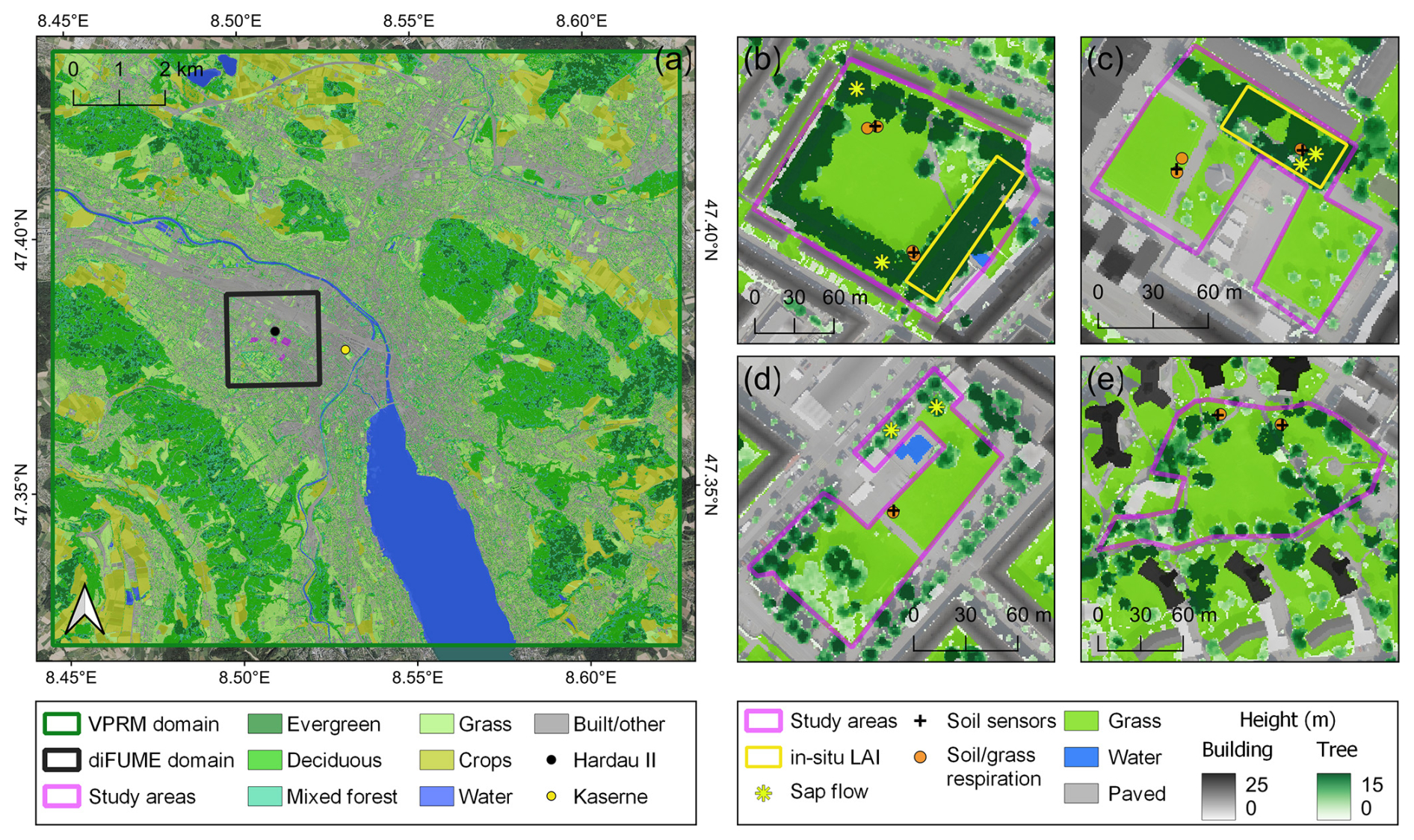
Figure 1 (a) Locations of the study areas, the meteorological stations (Hardau II, Kaserne), and the model domains over the land cover map of the Zurich region. Locations of the in situ observations in (b) Bullingerhof, (c) Hardaupark, (d) Fritschiwiese, and (e) Heiligfeld over the land cover map and with the building and tree heights overlaid. All maps are projected in the Swiss CH1903+/LV95 coordinate system (EPSG: 2056) in a semi-transparent format over a basemap of aerial orthophotos (Orthofoto, 2024).

2 Methods

2.1 Site description

The in situ observations were performed in four public parks in the city district Hard in Zurich, Switzerland, close to the Hardau II ICOS Cities tower site (Fig. 1). According to the climate normal of the period 1991–2020 from the weather station Fluntern (556 m a.s.l.; 47.38° N, 8.57° E), the annual total precipitation in Zurich is 1108 mm, with summer months being rainier than winter months, and the annual mean temperature is 9.8 °C, reaching a 24.3 °C monthly mean of daily maximum in July and a −1.4 °C monthly mean of daily minimum in January. The four parks are similar in size, land cover types, use, and management practices, but they differ in terms of age, tree species, tree size/age, and tree cover fractions (Table 1). Bullingerhof was developed in the 1930s and consists of rows of Platanus sp. trees, surrounding a large open lawn (Fig. 1b). Hardaupark is a more recently developed park. It features an old tree row of Platanus sp. in the northern part, which were planted in the 1970s, but the lawns (the main part of the park) are covered only by small trees, (Larix x marschlinsii and Robinia pseudoacacia), established in 2010 (Fig. 1c). Part of the lawn was previously a parking lot. Fritschiwiese was initially developed as a park in 1921, previously being part of the nearby cemetery. The northern part was redesigned in the 1970s due to underground constructions, which include energy generation units. Trees, featuring mainly Tilia sp., are scattered and mainly surround the lawn in the centre, and they were planted between the 1950s and 1970s (Fig. 1d). Heiligfeld was developed in 1955 and features a diverse array of tree species and ages, with Carpinus betulus, Betula pendula, Acer sp., Pinus sp., and Quercus sp. constituting the main park's tree population. Similarly to the other parks, the central area of the park consists of an open lawn (Fig. 1e). The four parks are neither irrigated nor fertilized throughout the year. Grass is mowed frequently during spring and summer, especially in the central areas of the parks, which are used by residents for recreation and sports. Some parts of the parks are not mowed, such as the eastern part of Heiligfeld.

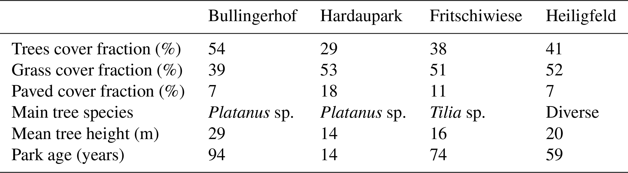
Table 1 Main characteristics of the parks used as study areas. The surface cover statistics are based on the land cover product (Sect. 2.4), and the tree information comes from the city tree inventory (Baumkataster Zurich, 2024).

2.2 In situ observations

2.2.1 Trees

Tree ecophysiological dynamics in the studied parks were monitored by measuring sap flux density on representative trees and the leaf area index (LAI) at dense tree stands. Six trees were equipped with heat pulse sap flow sensors (3×3 cm probes, Implexx Sense) in July 2022, providing continuous measurements at 10 min sampling intervals. The sensors, along with the boxes containing power and electronics, were installed on the tree trunks at 2.9–3.5 m height a.g.l. to avoid vandalism. One sensor per tree was installed, always facing south and placed beneath the tree branches (except the northern tree in Bullingerhof, where the sensor is above the lowest branch). Two trees per park – except Heiligfeld – were equipped with sap flow sensors: two Platanus sp. trees in Bullingerhof, two Platanus sp. trees in Hardaupark, and two Tilia sp. trees in Fritschiwiese (Fig. 1b–d). For each tree, the trunk diameter and the bark depth at installation height were measured at the time of installation. Heat velocity (m s⁻¹) was estimated from each sensor using the outer and inner needle thermistors at 0.5 and 1.5 cm sapwood depth using the heat ratio method and converted to sap flux densities (cm³ cm⁻² h⁻¹), as described in Forster (2019, 2021). The sap flux densities from the outer thermistors were consistently lower than the inner thermistors. Since sap flux density was used as a proxy for tree gross photosynthesis in this study, only the inner thermistor data were used in the analyses. The 10 min data per tree were averaged to hourly values per park to extract further statistics in this study. Given that sap flux density is controlled by similar environmental parameters to gross photosynthesis, these observations were treated in this study as a proxy for GPP.

The LAI was measured in dense tree stands, found only in Bullingerhof and Hardaupark (Fig. 1b, c). It was measured from April 2022 only during sunny conditions using a ceptometer (SS1 SunScan, Delta-T Devices). The measurement frequency depended on the sky conditions, optimally with weekly repetitions during leaf-on and leaf-off periods and biweekly during the rest of the growing period. The photosynthetically active radiation (PAR) above and below the tree canopy was sampled sequentially using the ceptometer probe. Above-canopy readings were sampled on the open lawns near the tree stands. The above-canopy incident total and diffuse PAR was sampled by casting a small shadow on part of the probe according to the instrument protocol (Webb et al., 2016). Between 15 and 20 below-canopy PAR readings were subsequently sampled every ∼2 m, standing in the centre of the stand minor axis and moving across the major axis holding the probe perpendicular to the direction of the sun. Above-canopy incident PAR was sampled again after the below-canopy readings to ensure that the light conditions did not change during each measurement cycle. The LAI of each stand was estimated according to the instrument software (Webb et al., 2016), assuming spherical leaf angle distribution and leaf PAR absorption of 0.85.

2.2.2 Lawns

The in situ measurements performed to monitor the park lawn dynamics included the installation of soil temperature (T_soil) and soil water content (SWC) sensors and the repeated measurement of soil and grass respiration. Seven soil sensors (TEROS 12, METER Group) were installed in May 2022 at different locations across the parks, with the central needle (temperature sensor) positioned at ∼15 cm depth. The sensitivity of the sensors to soil water content is contained within ∼1 L of soil volume around each sensor, installed along a vertical axis to increase the measurement volume along this axis. According to the installation characteristics and the sensor specifications, the measurement volume of the sensors was between 9 and 21 cm depth. The sensors were buried in the soil along with the electronics and communication boxes. This allowed the selection of the sensor locations without any restrictions. The communication was achieved through LoRaWAN sensor devices (Decentlab GmbH) with data transmission every 10 min.

Soil and grass respiration were measured near each soil sensor from July 2022 using a portable CO₂ soil efflux system equipped with a 20 cm diameter survey chamber (LI-8200-01S, LI-COR Biosciences) and a ${\mathrm{CO}}_{\mathrm{2}}/{\mathrm{H}}_{\mathrm{2}}\mathrm{O}$ analyser (LI-870, LI-COR Biosciences). Altogether, 10 soil collars were permanently installed at the four parks (Fig. 1), allowing repeated measurements at the exact same location under minimum soil disturbance. The collars were inserted completely into the ground to avoid any interference with the park visitors and the maintenance activities (e.g. grass mowing). A removable 20 cm diameter metal adapter of 3.5 cm height was used as a fixing between the top part of the soil collar and the survey chamber. Some of the collars were intentionally left undisturbed to measure total grass and soil respiration (R_eco). Conversely, the grass in the rest of the collars was removed to enable the isolated measurement of bare soil respiration (R_soil). Only R_eco was measured during the first two campaigns in summer 2022, then, gradually, grass was removed from eight collars to measure R_soil. Two R_eco collars were kept throughout winter (1× Hardaupark, 1× Heiligfeld), and two more (2× Bullingerhof) were established in June 2023. The aim of the different treatment strategies was to assess both bare soil respiration and lawn R_eco under similar environmental conditions. The CO₂ flux was calculated from the chamber measurements using an exponential fit to the increase in dry CO₂ concentration over time, while the chamber was closed using SoilFluxPro software (LI-COR Biosciences). The derivation of the CO₂ flux equation is described in detail in the LI-8200-01S manual (LI-COR, 2024). The total measurement time (chamber closed) was 2 min, and a deadband of 25 s was applied. At least two repeated observations were conducted at each collar to account for potentially problematic measurements. T_soil and SWC at 5 cm depth were measured at the same time, with the chamber measurements next to each collar with the survey chamber integrated soil probe (HydraProbe, Stevens) additionally to the permanent soil sensors at 15 cm, to get a more complete overview of the soil conditions. Measurements of R_eco and R_soil were performed during day campaigns (07:00–16:00 CET) every 2 weeks. The lawn measurement locations were selected to account for the variability in the environmental conditions and eventually in the soil and grass respiration fluxes across the parks. Sunny locations were selected in Bullingerhof, Hardaupark, and Fritschiwiese. Additionally, shaded or partly shaded locations were selected in Bullingerhof, Hardaupark, and Heiligfeld (Fig. 1).

2.3 Model description

Four different types of biosphere models were selected for this study; a full carbon cycling ecosystem model designed for natural ecosystems (JSBACH), a land surface model designed for urban areas (SUEWS), a satellite-based semi-empirical CO₂ flux model designed for urban areas (diFUME), and a satellite-based light use efficiency model initially designed for natural ecosystems (VPRM). The rationale behind the model selection was to investigate if their performance in simulating the urban CO₂ exchanges follows the level of sophistication (i.e. the model complexity and detail in simulating the processes that govern CO₂ exchanges) and at the same time to explore the advantages of the models that are specifically designed for urban applications over the ones designed for natural ecosystems. Furthermore, the selection of these models allows the comparison of different model attributes (e.g. satellite-based phenology versus modelled phenology) but also the identification of the challenges or drawbacks when applying models designed for natural ecosystems to urban environments. The models are described below in alphabetical order, and a more detailed overview of each model can be found in Appendix A.

2.3.1 diFUME

diFUME, taking its name from the project “Urban carbon dioxide Flux Monitoring using Eddy Covariance and Earth Observation”, is a recently developed urban CO₂ flux model (Stagakis et al., 2023b), which uses a semi-empirical approach for modelling the biogenic CO₂ fluxes in urban areas based on the main environmental controlling parameters of photosynthesis and respiration processes (i.e. incoming global radiation, air–soil temperature, vapour pressure deficit, and soil water content), capturing the spatiotemporal dynamics of plant phenology using high-resolution satellite imagery and simulating the effects of urban morphology on the canopy radiation interception based on a voxel traversal (ray tracing) algorithm (Fig. A1). The study area is represented in three dimensions as a 3D grid of voxels of certain size (5 m in this application) and category (i.e. terrain, building, vegetation, and air) according to the digital surface model (DSM) and land cover information. GPP is modelled for the vegetation voxels of each horizontal layer (i) based on the PAR reaching the sunlit and shaded fraction of the LAI in each voxel using a non-rectangular hyperbolic function and other empirical functions for the simulation of air temperature, vapour pressure deficit, and soil water content effects. R_eco is separated into the aboveground and belowground components: the aboveground component is modelled based on an exponential fixed-Q₁₀ equation using air temperature, multiplied by the LAI, and the belowground component is based on a modified Arrhenius equation using soil temperature and soil water content. The main equations used by diFUME, along with a model flow diagram, are presented in Appendix A. The model version applied in this study contains some modifications compared to the version described in Stagakis et al. (2023b), such as the addition of a sky-view factor (SVF) estimation module using the voxel traversal algorithm, the addition of a module to split global radiation into its diffuse and direct components, and the simplification of the equations for the estimation of the diffuse and reflected PAR reaching the leaf surface of each vegetation voxel (i.e. directional SVFs and SVFs including tree canopies are not used in this version).

The model inputs used in this study are the land cover map, meteorology, and DSMs, as described in Sect. 2.4. The LAI dynamics come from the Copernicus High Resolution Vegetation Phenology and Productivity (HR-VPP) product, which includes four daily vegetation indices (PPI, NDVI, LAI, and FAPAR) and quality information at 10 m resolution. The Copernicus LAI product was filtered per pixel according to the quality flags for clouds, cloud shadows, proximity to clouds, and cloud shadows and snow, resampled to 5 m according to the land cover information (Stagakis et al., 2023b), and a 16 d maximum value composite filter was applied to exclude bad values and gaps. The 16 d product was then linearly interpolated to derive 5 d LAI values, which are used as model inputs. The maximum acceptable LAI value over grass pixels was set to 3 m² m⁻², since the park grass is frequently mowed.

2.3.2 JSBACH

JSBACH, standing for “Jena Scheme for Biosphere–Atmosphere Coupling in Hamburg” (Reick et al., 2013), is the land component in the Earth system models of the Max Planck Institute for Meteorology that simulates terrestrial energy, hydrology, and carbon fluxes utilizing a number of submodels (Fig. A2). The vegetation is described by plant functional types (PFTs). In this study, the vegetation was described by the C₃ grass and broadleaved deciduous tree PFTs. The carbon assimilation is described by the biochemical photosynthesis model of Farquhar et al. (1980). The assimilation rate is limited either by the carboxylation rate (J_C,stress) or by the electron transport rate (J_E,stress) (Table A1). J_C,stress is a function of the maximum carboxylation rate (V_max), which has an Arrhenius-type temperature dependence, and J_E,stress is a function of PAR (non-rectangular hyperbolic dependence) and J_max (maximum electron transport rate), which has a linear dependence on temperature. Both V_max and J_max are inhibited above 55 °C. V_max is also scaled with a factor depending on the canopy depth to account for the Rubisco profile in the canopy. Dark respiration (r_d) is a fixed fraction of V_max at 25 °C with an Arrhenius-type temperature dependence. It is inhibited above 55 °C and decreases with increasing solar irradiance. The unstressed stomatal conductance ($g_{\mathrm{L}}^{{\mathrm{H}}_{\mathrm{2}}\mathrm{O}}$) is scaled by the plant available soil water (f_ws) to obtain stomatal conductance under water stress ($g_{\mathrm{L},\mathrm{stress}}^{{\mathrm{H}}_{\mathrm{2}}\mathrm{O}}$), which is used to derive J_C,stress and J_E,stress and then finally the assimilation rate under water stress (A_stress). f_ws depends on soil moisture in the root zone and specific humidity. The seasonal development of the LAI is described by the Logistic Growth Phenology (LoGro-P) model (Böttcher et al., 2016). The development of the LAI of broadleaved deciduous trees is described by the summer green phenology (Table A1). It has three phases: the growth period in the spring (k>0 and p=0), the vegetative phase during the summer (k=0 and small p), and the rest phase starting in autumn (k=0 and high p). The transition from the rest phase to the growth phase is dependent on the evolution of the temperature using the alternating model of Murray et al. (1989), while the growth phase has a fixed duration. The maximum LAI is given as a parameter. The grass phenology further includes soil moisture and net primary productivity (NPP) as determining factors. In the autumn, the phase transition occurs when the pseudo-soil temperature (running mean of air temperature) falls below a critical soil temperature, while grasses grow when there is sufficient soil moisture and temperature. Leaves are shed when NPP is negative. The soil hydrology parameters are set on the basis of soil texture. The soil moisture is simulated with five layers within a multilayer soil hydrological scheme. The dynamics of litter and soil carbon are described by the submodel Yasso07 (Tuomi et al., 2009, 2011). Five carbon pools are distinguished based on their chemical properties (acid-hydrolysable, water-soluble, ethanol-soluble, neither hydrolysable nor soluble, humus). The first four pools (a, w, e, n) are tracked both above and below ground, and separate pools are used for woody and non-woody litter – altogether 18 pools. The litter pools receive carbon input from vegetation through the litter flux, faeces from grazing, and losses from the reserve pool (Table A1). Decomposition of the litter pools causes carbon to transfer between the pools and to the atmosphere. The loss rates depend on temperature, water availability, and the type of litter elements. JSBACH is forced by air temperature, total precipitation, short-wave and long-wave radiation, air humidity, wind speed, and CO₂ concentration, as described in Sect. 2.4.3.

2.3.3 SUEWS

The Surface Urban Energy and Water Balance Scheme (SUEWS; Järvi et al., 2011, 2019) is an urban land surface model jointly simulating the surface energy and water balances and carbon dioxide surface exchange at the local or neighbourhood scale (Fig. A3). SUEWS encompasses various submodels, which account for factors like net all-wave radiation, heat storage (Grimmond et al., 1991; Sun et al., 2017), anthropogenic heat flux, irrigation, roughness layer temperature, and relative humidity (Tang et al., 2021). These submodels are essential for accurately representing urban characteristics affecting the simulated balances and exchanges. Photosynthetic uptake is calculated using an empirical canopy-level photosynthesis model, where the potential photosynthesis is modified for different environmental factors (Table A1). The same environmental factors also control the surface (stomatal) conductance. The seasonal development of the LAI depends on the growing degree days (GDD) and senescence degree days (SDD), which depend on air temperature. The rates of leaf-on, leaf-off, and maximum LAI are given as an input. During the leaf-on period, the LAI remains relatively stable and responds slowly to stress conditions. In contrast, other environmental factors that regulate surface conductance exhibit more pronounced responses to stress. Soil and vegetation respiration is calculated as simple exponential dependence on air temperature. SUEWS provides a holistic approach to joint energy, water, and CO₂ cycles in urban environments, allowing us to account, for example, for the influence of elevated air temperatures on water and CO₂ cycles. The model relies on standard meteorological inputs like wind speed, air temperature, air pressure, precipitation, and short-wave radiation. The forcing air temperature needs to be from above the roughness sublayer, so, in this study, the measured 2 m air temperature is scaled to 35 m using a lapse rate of 6.5 °C km⁻¹. SUEWS is able to calculate 2 m temperature from the forcing temperature (Tang et al., 2021), which is used in the calculations of photosynthesis and soil and vegetation respiration. Additionally, site-specific data, such as surface cover fractions and tree and building heights, are needed. SUEWS has extensively been evaluated in simulating urban CO₂ exchanges in various cities, including Helsinki, Minneapolis, Swindon, and Beijing (Havu et al., 2022; Järvi et al., 2019; Zheng et al., 2023). For this study, we employed the latest available version, SUEWS V2020a, using the land cover, meteorology, and surface morphology inputs described in Sect. 2.4.

2.3.4 VPRM

The Vegetation Photosynthesis and Respiration Model (VPRM) is a satellite-based, data-driven model to estimate spatial and temporal surface biogenic CO₂ fluxes for different plant functional types (Mahadevan et al., 2008) (Fig. A4). VPRM represents the NEE of CO₂ as a combination of two components: GPP and R_eco. GPP is a light-dependent term using remote sensing vegetation indices, including the Enhanced Vegetation Index (EVI) and Land Surface Water Index (LSWI), combined with short-wave solar radiation to estimate the carbon uptake from photosynthesis. R_eco is a light-independent part using only temperature at 2 m above the ground and a linear model to denote the carbon emission from the ecosystem respiration (Table A1). Additionally, the VPRM requires an accurate vegetation cover map to provide the spatial distribution of different vegetation types and utilizes distinct parameters for different vegetation types to drive the VPRM. These parameters are fitted by using the NEE observations from eddy covariance towers that monitor specific vegetation types. VPRM has been widely applied across Europe to estimate the large-scale biogenic CO₂ fluxes (Ahmadov et al., 2009; Gerbig and Koch, 2023; Zhao et al., 2023).

For the vegetation indices, we used the Sentinel-2 MSI Level-2A (MAJA Tiles) product (10 m spatial resolution) provided by the German Aerospace Center (DLR, 2019). The vegetation cover is taken from our self-developed vegetation land cover product, which is described in Sect. 2.4.1, and has been resampled to align with the Sentinel-2 image grid. Temperature and short-wave downward solar radiation data are sourced from the Zurich Kaserne station (Sect. 2.4.3). The plant-type-specific parameters for VPRM are those presented by Zhao et al. (2023).

2.4 Data inputs

2.4.1 Land cover

For the accurate modelling of high-spatial-resolution biogenic fluxes, a precise and high-resolution vegetation land cover map is needed for diFUME, SUEWS, and VPRM (Table 2). The following high-quality datasets available in Zurich made this objective possible:

• a.

  Land Use Cadastre of the Canton of Zurich (Amtliche Vermessung, 2024). This detailed GIS dataset is the official land registry of the Canton and the basis for geographical information in almost all domains from spatial planning to agriculture and tourism. It acted as our base map, with vegetation types reclassified to distinguish between grassland and cropland areas. Note that the “closed forest” was assigned to grassland, since it was replaced by more accurate tree cover data later while also retaining the grassland information within the forests.

• b.

  Urban Atlas (Urban Atlas, 2018). For deriving the cropland coverage, we utilized the Urban Atlas 2018 from the Copernicus Land Monitoring Service. This dataset discriminates between crop and grass fields, which was not possible based on the Canton Cadastre alone.

• c.

  Vegetation Height Model (VHM) from the Swiss federal forest inventory (Vegetationshöhenmodell LFI, 2019). This dataset is based on a combination of stereo aerial images and lidar observations and is available for the whole country at a resolution of 1 m × 1 m. Pixels indicating trees shorter than 2 m were excluded from this dataset, as these pixels, based on our observations, are often noisy signals.

• d.

  Forest Mixture from the Swiss Federal Forest Inventory (Waldmischungsgrad LFI, 2018). This dataset derives the forest mixture ratio based on Sentinel-1 and Sentinel-2 satellite observations and is available for the whole country at a resolution of 10 m × 10 m. Two empirical thresholds were used to convert the forest mixture ratio to three tree types: deciduous (greater than 80 %), mixed forest (between 20 % and 80 %), and evergreen (less than 20 %). Within the city of Zurich, a large majority of trees are deciduous.

We merged tree classifications with the VHM to produce a detailed tree species cover map. Areas that were unidentifiable, often found in urban regions, were labelled as deciduous. The generated tree species cover map was then combined with the other datasets, resulting in our 1 m resolution land cover map for Zurich.

2.4.2 Digital surface models

The very-high-resolution DSM products (terrain, building, and tree heights) developed by the Zurich city authorities (Baumhöhen, 2023; Digitales Oberflächenmodell, 2022; Digitales Terrainmodell, 2022) were used in this study as inputs for diFUME and SUEWS (Table 2). The DSM products are derived from high-resolution laser scanning (lidar; average point density of 16 points m⁻²) over the years 2021 and 2022.

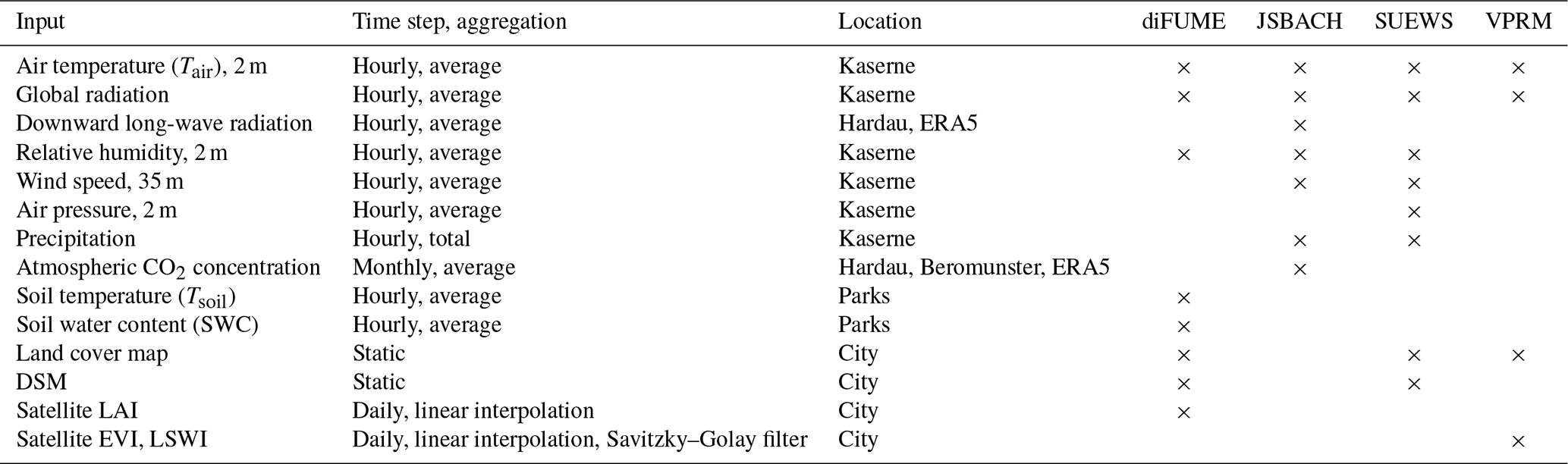
Table 2 Overview of data inputs required by each model during the simulation period January 2022–September 2023.

2.4.3 Weather driver data

We used meteorological measurements mainly from the site Zurich Kaserne (January 2022–September 2023), which is a station of the Swiss National Air Pollution Monitoring Network (NABEL). The measurements are performed with the same high-quality instruments as used in the national weather observation network SwissMetNet. Zurich Kaserne is located in a large courtyard at a distance of about 1–1.5 km from the parks analysed in this study (Fig. 1). The measurements from Zurich Kaserne are expected to be representative for the parks, as it is located in a similar urban setting. Wind and global radiation are measured on top of a neighbouring four-storey building. Wind is measured at 35 m, and global radiation is measured at 27 m above ground. Additionally, downward long-wave radiation and atmospheric CO₂ concentration data were derived for the period July 2022–September 2023 from the ICOS Cities Hardau II station (110 m a.g.l.). For the period prior to the Hardau II installation (January 2022–June 2022) and for the spin-up period of JSBACH (1950–2021), the Copernicus ERA5-Land dataset was used to derive all missing observations, with the exception of CO₂ concentration, which was derived from Beromunster station (November 2012–February 2022) and prior to that from a global gridded monthly dataset of CO₂ (Cheng et al., 2022). The CO₂ data were used in JSBACH as monthly means. The meteorological measurements used as input for the models during the simulation period January 2022–September 2023 are listed in Table 2. diFUME additionally requires T_soil and SWC, which were measured in seven locations across the studied parks as described in Sect. 2.2.2.

2.5 Model comparison and evaluation

All models were run for the period January 2022–September 2023 for the four parks using the hourly meteorological inputs as described in Table 2. diFUME and VPRM ran spatially at high resolution (5 and 10 m, respectively), while SUEWS and JSBACH provided integrated simulations for each land cover type of each park. This intercomparison study focuses on the park trees and lawns separately. To compare between the spatial and integrated model simulations, the grass and tree pixels of each park from diFUME and VPRM outputs were selected according to the land cover map. All pixels covered by at least 90 % by a given land cover type based on the 1 m land cover map were selected and averaged for each park. Hourly GPP, R_eco, and NEE estimates for each park were then temporally averaged to daily, monthly, or annual values. CO₂ flux units were kept uniform across the article ($\mathrm{\mu }\mathrm{mol}{\mathrm{m}}^{-\mathrm{2}}{\mathrm{s}}^{-\mathrm{1}}$), except for the annual totals, where the units were converted (to kg m⁻² a⁻¹) to facilitate the comparison with the relevant literature. In this study, we kept GPP and R_eco positive for easier plotting and comparison and estimated NEE as NEE = R_eco−GPP.

Given the available in situ observations, which do not cover all carbon cycle components and drivers due to technical and logistical restrictions, we focused on the evaluation of tree LAI and GPP and of SWC and R_eco in the lawns. Modelled LAI can be directly evaluated using the field observations in the measured tree stands. However, VPRM does not include the LAI in the light use efficiency equation but uses EVI as a proxy of vegetation greenness. Therefore, and in order to achieve uniform evaluation across the four models, we converted EVI to LAI using a linear regression (R²=0.86, slope = 7.03, intercept = −1.26) between the HR-VPP LAI and Sentinel-2 EVI for all cloud-free acquisitions within the study period using the mean values over trees of each park. A similar approach was adopted for the evaluation of tree GPP using sap flow as a proxy. Since the diurnal behaviour of sap flow is expected to be quite different from GPP, the evaluation was performed using daily integrated values. The daily averaged sap flow values (cm³ cm⁻² h⁻¹) were converted to GPP ($\mathrm{\mu }\mathrm{mol}{\mathrm{m}}^{-\mathrm{2}}{\mathrm{s}}^{-\mathrm{1}}$) by a linear regression (R²=0.81, slope = 0.77, intercept = 1.93) between the mean GPP by the four models over the four parks and the mean sap flow of all sampled trees.

The SWC observations and model estimates cannot be directly compared because of different soil layers considered and different soil parameterizations. Specifically, the observations were representative of approximately 9 to 21 cm soil depth, which can be closely compared to one soil layer simulated by JSBACH but cannot be directly compared with SUEWS because the latter estimates a bulk SWC value for the total simulated soil volume. Furthermore, different soil parameterizations in the models can lead to different absolute maximum and minimum SWC values, which makes the direct comparison difficult (Fig. B1c). Therefore, the daily means of SWC observations and model estimates were normalized according to the individual time series maximum and minimum values to avoid the effects of different model parameterizations for soil and the effects of different soil depths measured and modelled. By applying this normalization on SWC time series, we focused on the evaluation of the temporal variability in each model rather than the absolute values. For VPRM, LSWI was used in this analysis as a proxy of SWC. Finally, lawn R_eco was evaluated using the averages of the in situ measurements for each daily campaign and the averages of the model outputs for the same days considering only the hours during the times of the measurements.

For the parameter evaluations, the average simulated value of the four parks (tree or lawn according to the parameter) of each model was compared to the average of the available observations, except for the LAI, for which only simulations at Bullingerhof and Hardaupark were used, and for R_eco, for which the observations at sunny and shaded locations (see Sect. 2.2.2) were averaged separately and the average of the two was regarded as the representative R_eco value to be compared with the models. The quantitative evaluation analysis in this study is presented using Taylor diagrams, combining three performance metrics: the normalized standard deviation, the correlation coefficient, and the centred root-mean-square error (Taylor, 2001).

2.6 Uncertainty analysis

As a simple measure of model uncertainty of the different biogenic CO₂ flux components (GPP, R_eco, NEE), we computed the standard deviation of each hourly value of the four models. The hourly time series of standard deviations were further aggregated to seasonal and diurnal patterns to examine the magnitude and significance of the biogenic model uncertainties. In order to address the importance of the biogenic CO₂ fluxes and their uncertainties in relation to the magnitude of the anthropogenic emissions, we focused on a central part of the city of Zurich corresponding to the diFUME domain (Fig. 1) and estimated the monthly anthropogenic emissions, considering building heating, industry, vehicle traffic, and human respiration. The monthly biogenic CO₂ fluxes (GPP, R_eco, NEE, averages of the four models) were scaled to the 2 km × 2 km domain according to the tree and grass land cover fractions and assuming that the tree and lawn simulations of the four parks are representative of the vegetation of the domain. The anthropogenic emissions for the specific area were estimated from the gridded annual inventory of the city of Zurich (Emiproc, 2024; Emissionskataster, 2024). For both anthropogenic and biogenic fluxes, the monthly average of the 2 years of the study was estimated.

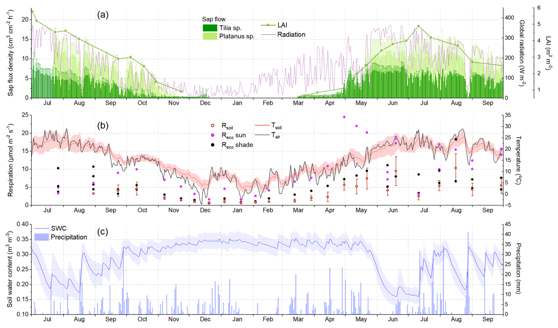
Figure 2 Time series of the in situ observations in the study parks (Fig. 1) during the campaigns from May 2022 to September 2023. (a) Average leaf area index (LAI) from the two Platanus sp. stands, daily averages and standard deviations of the sap flux densities per tree species, and daily average incoming global radiation. (b) Average and standard deviation of the measured soil respiration (R_soil), measured lawn ecosystem respiration (R_eco) (sunny and shaded locations in different colours), and daily average air and soil temperatures, where the shading refers to the standard deviation of the seven soil sensors. (c) Daily average (line) and standard deviation (shade) of the measured soil water content (SWC) and daily precipitation (bars).

3 Results

3.1 In situ observations

Tree LAI and sap flow observations provided detailed information on tree phenology and physiology (Fig. 2a). The phenology of the Platanus sp. stands was somewhat different in the 2 study years. In 2022, leaf growth started in mid-April, and, already by mid-May, the LAI had reached nearly 4 m² m⁻² (Fig. B1a). The peak was at the end of June, reaching around 5.5 m² m⁻². Then, the LAI gradually declined until the end of November when the leaf fall was completed (Figs. 2a, B1a). In 2023, the leaf growth started around the same time as in 2022 but was considerably slower. By mid-May, the LAI had only reached about 2.5 m² m⁻², and it peaked at the beginning of July at a lower value than in 2022 (∼4.5 m² m⁻²). The different phenological patterns observed in the 2 studied years were also confirmed by the satellite indices (Fig. B1a).

Sap flux density observations of the Platanus sp. followed the observed LAI seasonality but were very variable according to the environmental conditions, co-varying strongly with incoming radiation, especially during summer periods (Fig. 2a). Sap flux density of the Tilia sp. showed similar seasonal variability but consistently lower values except during spring 2023, when Tilia sp. trees had apparently earlier leaf growth than the Platanus sp. trees. On the other hand, Tilia sp. trees dropped their leaves a bit earlier than Platanus sp. trees according to the sap flow observations during October and November 2022 (Fig. 2a). The effects of the drought periods (Fig. 2c) on the sap flow are not clearly discernible in Fig. 2a; however, there was an increase in sap flow visible after the rains at the middle of August 2022.

The measurements at the park lawns provided valuable insights into the seasonal dynamics of grass and soil respiration. R_soil seasonal variability consistently followed T_soil and SWC changes (Fig. 2b, c). Applying a modified Lloyd and Taylor (1994) equation fit to the R_soil observations, their variability was explained to 64 %–72 % by the T_soil and SWC observations. R_soil was low during winter, rose in spring, and reached high values during hot summer days if soil moisture was available (Fig. 2b). During summer, conditions were more variable depending on the park location and hour of measurement; therefore the measured R_soil varied significantly. The highest R_soil was measured during June and August 2023, reaching values above 10 $\mathrm{\mu }\mathrm{mol}{\mathrm{CO}}_{\mathrm{2}}{\mathrm{m}}^{-\mathrm{2}}{\mathrm{s}}^{-\mathrm{1}}$. The high value in June, which occurred during a rain event, is bracketed by much lower values during the prolonged drought period in June/July 2023.

Lawn R_eco followed roughly the same seasonal pattern as R_soil but with consistently higher values (Fig. 2b). Moreover, the variability observed in R_eco between the different collars was very intense. This was to be expected, since the grass biomass, which contributed to the measured flux, was variable according to the park location. The general tendency observed on site was that the shaded or partly shaded locations tended to have less thick and dense grass cover than the sunny locations. This was confirmed in the measurements by comparing shaded R_eco with R_soil. The differences were not very big in the majority of the cases, indicating that R_soil was the main source at these locations. On the other hand, shaded locations did not dry out as quickly as the sunny locations during drought conditions, maintaining the required soil moisture for healthy aboveground leaf biomass. Therefore, it was observed in the measurements that shaded R_eco was sometimes higher than sunny R_eco during summer (Fig. 2b). However, the grass in sunny locations tended to recover quickly after rain events that restored the SWC during summer and autumn. Another important parameter to consider when interpreting the R_eco observations is the grass mowing. Mowing has been reported to induce high respiration rates (Allaire et al., 2008; Kaye et al., 2005), which is the most probable explanation of the very high R_eco measured in the sunny lawn locations since the end of April 2023 and during summer months (Fig. 2b). The highest R_eco values were found in the sunny location in the Hardaupark, which is the most recently constructed park in this study. Fitting the modified Lloyd and Taylor (1994) equation to the R_eco measurements showed that the observed variability can be explained only to 38 % by measured T_soil and water content.

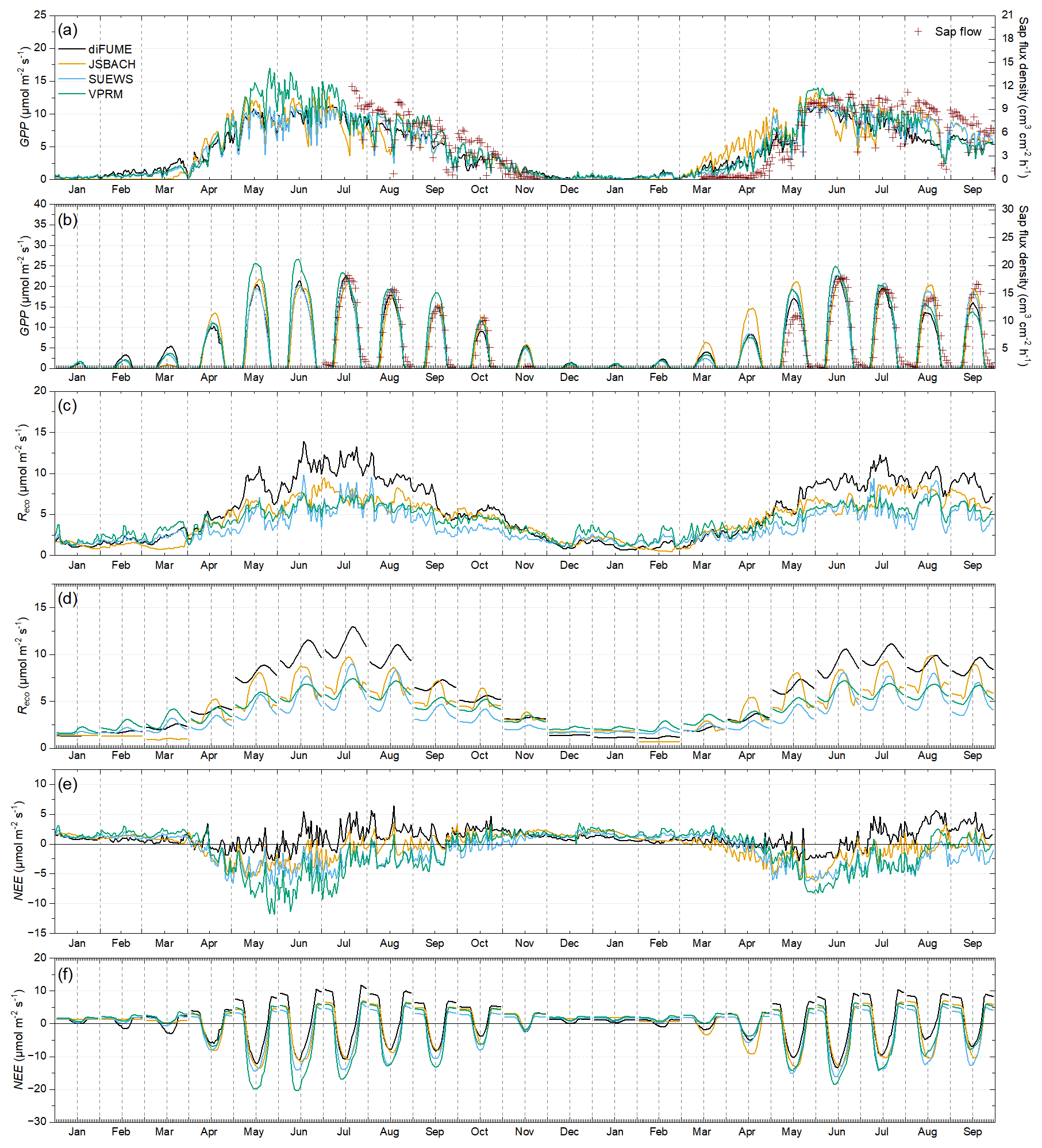
Figure 3 Time series of model outputs for park trees (averages of the four parks). Daily averages of (a) gross primary production (GPP), (c) ecosystem respiration (R_eco), and (e) net ecosystem exchange (NEE) estimates and diurnal hourly averages per month of (b) GPP, (d) R_eco, and (f) NEE estimates. Sap flux density observations (averages of all trees) per day and hour are plotted over GPP in panels (a) and (b).

3.2 Model comparison

The GPP, R_eco, and NEE outputs of the four models were compared for park trees (Fig. 3) and lawns (Fig. 4). Figures 3 and 4 contain time series of daily totals and hourly diurnal averages of each month for each modelled parameter. Observed tree sap flow and lawn R_eco are plotted against modelled tree GPP (Fig. 3a, b) and modelled lawn R_eco (Fig. 4c), respectively. In general, models seemed to better agree for park trees than lawn. Tree GPP estimates were surprisingly consistent between the four models (Fig. 3a, b). Exceptions were the higher VPRM estimates between mid-May and mid-July 2022 and the higher JSBACH estimates during mid-March to mid-May 2023. A considerable deviation between the models was also observed during August and September 2023, when diFUME and VPRM showed lower GPP than the other two models. Using sap flow as a GPP proxy, it was observed that the tree phenological and physiological seasonal dynamics were captured well by the models (Fig. 3a). The modelled diurnal GPP profiles also agree well with the sap flow observations, even though there were some differences in the timing (i.e. sap flow peaked later than GPP) as expected. However, there was considerable overestimation of spring GPP, especially during April and the beginning of May 2023.

Lawn GPP estimations did not match well between the models (Fig. 4a, b). VPRM and JSBACH showed high lawn GPP during spring and early summer and strong variability from day to day according to daylight conditions. diFUME and SUEWS presented more conservative lawn GPP estimates, much lower than the other two models, and not such intense day-to-day variations. During mid-July–August 2022, all models captured the drop in lawn GPP due to drought conditions, with JSBACH showing reduced sensitivity of GPP to drought compared to the other models. During summer 2023, VPRM showed a very intense drop in lawn GPP from the beginning of June due to drought conditions (see Fig. 2) and only a slight recovery after mid-July (Fig. 4a). Such intense variability was only captured by JSBACH, which simulated intense drops and fast recoveries after rain events during the whole summer of 2023. GPP seasonality in VPRM is mainly driven by the satellite EVI.

Simulated R_eco seasonal variability agreed well between the four models (Figs. 3c, 4c). diFUME showed distinctly higher R_eco for trees during summer, while SUEWS showed lower R_eco for lawns compared to the other models. diFUME showed very similar R_eco estimated for lawns and trees, which was also the case for GPP, because, in contrast to the other models, the parameterization was the same for all plant types in the version used in this study. The rest of the models showed higher R_eco for lawns during summer compared to trees. The diurnal patterns of R_eco were slightly different between the models (Figs. 3d, 4d). JSBACH peaked earlier in the day and diFUME peaked later in the afternoon compared to the other models. Moreover, diFUME tended to show higher R_eco at night compared to the other models, most probably because T_soil is the main driver of R_soil in this model instead of T_air. None of the models seemed to capture any distinctive drought effect on lawn R_eco (Fig. 4c). When compared to the lawn R_eco observations, it appeared that the simulated values were closer to the shaded collar observations, while the sunny collar observations were much higher than the simulations during most of the time, except during drought conditions, when simulations were higher than the observations. It must be noted here that the comparison between observations and simulations shown in Fig. 4c is not entirely accurate because the observations were taken during a specific time of day and the daily averages take into account only the observation times. More detailed comparisons between R_eco observations and simulations are presented in Fig. B2d. Overall, it can be deduced that all models were conservative in their lawn R_eco estimations and underestimated the full potential of R_eco in open sunny park areas with thick managed lawn under wet and warm conditions.

NEE estimates of each model showed more distinctive seasonal and diurnal patterns compared to GPP and R_eco alone (Figs. 3e–f and 4e–f). For both trees and lawns, VPRM showed the strongest (most negative) NEE values during spring and summer, except during late summer periods for lawns, when daily NEE turned abruptly to high positive values. diFUME was the most “conservative” model, with daily NEE values close to zero during the whole growing period for trees and lawns, with late summer NEE turning towards more positive values due to the drop in GPP and the consistently high R_eco. The daily NEE of JSBACH and SUEWS was intermediate between diFUME and VPRM estimates. In contrast to the rest of the models, SUEWS showed very different NEE estimates between trees and lawns, with trees estimated as more productive than lawns. The diurnal NEE patterns were very much alike between the four models (Figs. 3f, 4f), but diFUME showed distinctively higher nighttime NEE values during spring and summer, especially for tree areas, while SUEWS diurnal lawn NEE amplitude was particularly smaller than the other models.

The annual totals estimated from each model are presented in Fig. 5. There was good agreement for the total tree GPP but not for tree R_eco, where diFUME estimated the highest and SUEWS estimated the lowest total R_eco (Fig. 5a). As a result, diFUME estimated that park tree areas acted as sources of CO₂, while SUEWS estimated them to be sinks. JSBACH NEE was very close to zero, with a standard deviation that spanned between positive and negative values, while VPRM showed high GPP variability between parks and the standard deviation of NEE also ranged between positive and negative values. For the lawns, SUEWS showed distinctively lower total GPP and R_eco compared to the other models. JSBACH and VPRM agreed well in the totals of GPP and R_eco, but VPRM showed much higher variability in total GPP. diFUME showed similar total lawn R_eco with JSBACH and VPRM but lower total GPP. In total, all models agreed that park lawns acted as CO₂ sources. However, for VPRM, the standard deviation was high and ranged between negative and positive values.

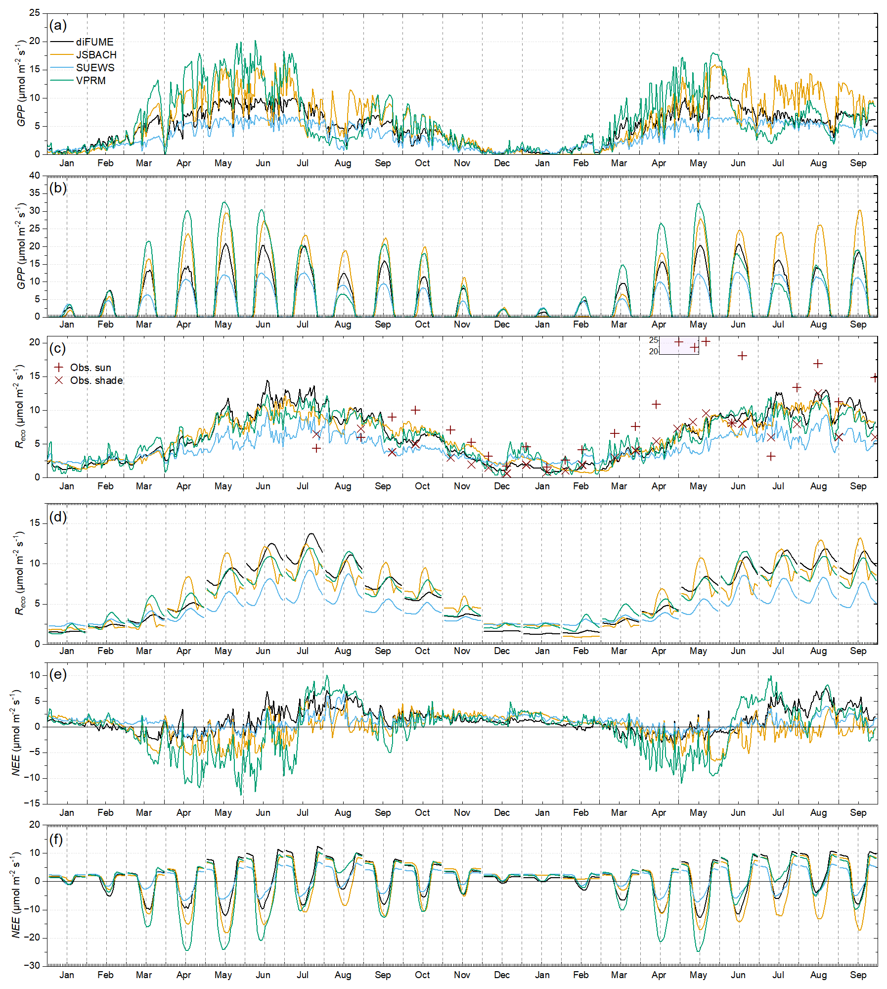
Figure 4 Time series of model outputs for park lawns (averages of the four parks). Daily averages of (a) gross primary production (GPP), (c) ecosystem respiration (R_eco), and (e) net ecosystem exchange (NEE) estimates and diurnal hourly averages per month of (b) GPP, (d) R_eco, and (f) NEE estimates. The observations of lawn R_eco (averages of sunny and shaded locations per campaign presented separately) are plotted over modelled R_eco in panel (c).

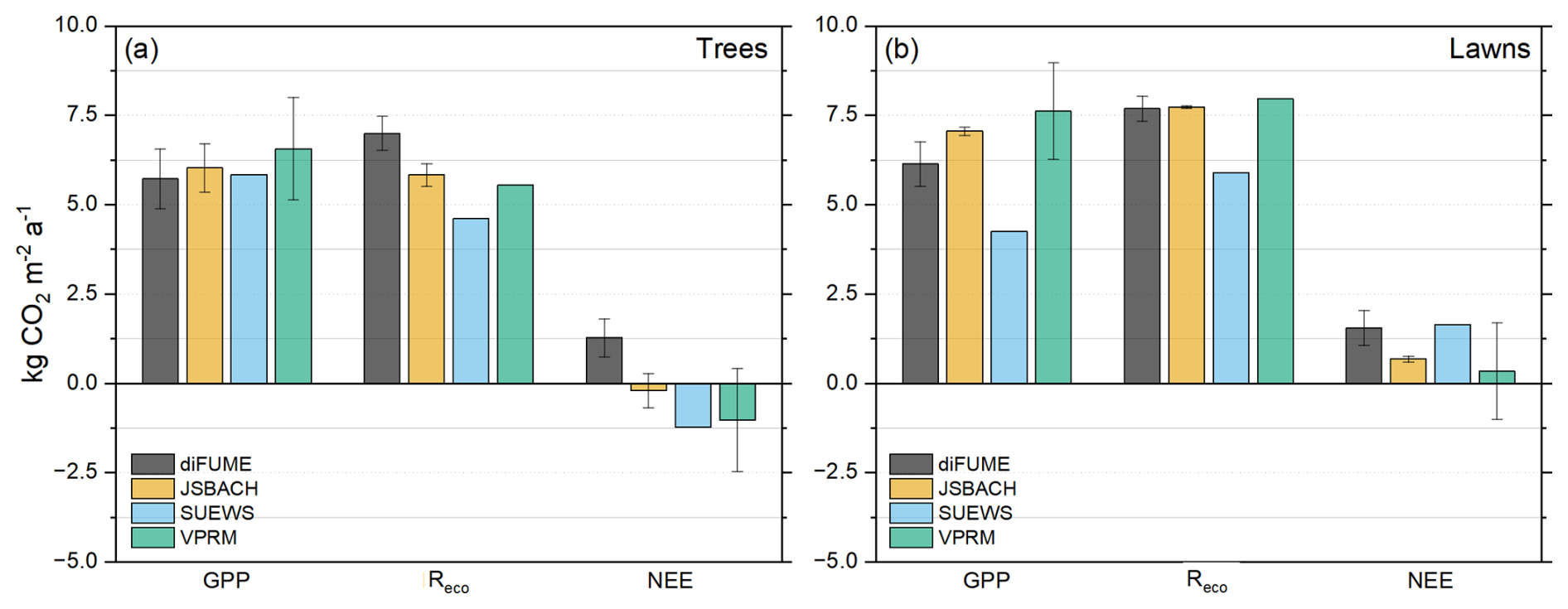
Figure 5 Annual totals for gross primary production (GPP), ecosystem respiration (R_eco), and net ecosystem exchange (NEE) for (a) trees and (b) lawns of the study parks. The whiskers express the standard deviation between the four parks. The period used to estimate the totals is July 2022 to June 2023.

3.3 Model evaluation

The Taylor diagrams provide a comprehensive intercomparison of the performance of the four models (Fig. 6). We focus only on certain parameters according to the available in situ observations, as described in Sect. 2.5. It can be observed in Fig. 6a that all models underestimated the tree LAI, but the two satellite-based models (diFUME and VPRM) captured the dynamics of the tree LAI better than the process-based models (SUEWS, JSBACH), which showed lower correlations with the observations. More specifically, all models underestimated the high LAI values during mid-summer, while SUEWS consistently overestimated the tree LAI during the rest of the seasonal cycle (Figs. B1a, B2a). However, the performance with respect to the LAI did not necessarily reflect on tree GPP simulation performance, since all models captured the measured daily sap flow variability well (Figs. 6c, 3a), with the best performance demonstrated by SUEWS and the worst demonstrated by JSBACH, most probably because of the early onset of GPP in JSBACH during spring 2023 (Fig. 3a). The lawn SWC variability (normalized) was captured very well by JSBACH and SUEWS (Fig. 6b), with the latter being a bit slower in the response to dryness and rain events (Fig. B1c), most probably because SUEWS does not simulate multiple soil layers as JSBACH does. On the contrary, satellite-based SWC estimation by VPRM did not perform equally well. Even though LSWI roughly detected the dry periods during summer, it was not so accurate when it came to fast responses of SWC to rain events and revealed unrealistically low SWC during winter (Fig. B1c). All models underestimated lawn R_eco (Fig. 6d), especially SUEWS, while JSBACH showed better performance compared to the other models. The reason for the underestimation is mainly the high values of measured R_eco in the fully sunlit park areas during spring 2023 (Figs. 2b, 4c, B2d).

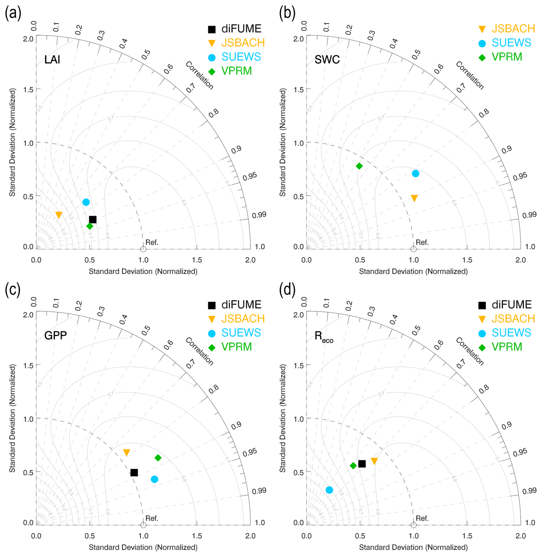
Figure 6 Taylor diagrams describing the model performance in capturing the variabilities in (a) tree leaf area index (LAI), (b) lawn soil water content (SWC), (c) tree gross primary production (GPP), and (d) ecosystem respiration (R_eco) of lawns. The Taylor diagrams combine three performance metrics: the standard deviation (x and y axes, grey concentric cycles), the correlation coefficient (azimuth angle, grey lines), and the centred root-mean-square error (dashed orange concentric cycles) (Taylor, 2001). The reference observation is plotted on the x axis according to its standard deviation (red square), and the distance from this point is inversely related to the performance of each model (coloured dots).

3.4 Biospheric flux uncertainty based on model spread

The dynamics of the estimated model uncertainties are presented in Fig. 7. Tree areas clearly showed lower uncertainties compared to lawns, mostly because of the increased inconsistencies between the models in the estimation of lawn GPP (Fig. 7b). The uncertainties for lawn GPP were highest during spring, reaching an average of around 9 $\mathrm{\mu }\mathrm{mol}{\mathrm{m}}^{-\mathrm{2}}{\mathrm{s}}^{-\mathrm{1}}$ at midday. Tree GPP uncertainties were highest during summer, reaching around 4 $\mathrm{\mu }\mathrm{mol}{\mathrm{m}}^{-\mathrm{2}}{\mathrm{s}}^{-\mathrm{1}}$ (Fig. 7a). Interestingly, the monthly diurnal patterns of GPP uncertainties of trees during the leaf-on period were different from lawns, presenting the highest values early in the morning or late in the afternoon rather than at midday. Early-morning peaks in tree GPP uncertainty appeared in June and July, while, during the rest of the growing season, the peaks appeared mostly during the afternoon (Fig. 7a). This pattern is the result of differences in the diurnal evolution of GPP, with some models having the maximum earlier in the day or showing wider peaks than others. R_eco uncertainties were similar in magnitude and pattern between trees and lawns (Fig. 7). They followed the seasonal growth of R_eco with higher values during warm months. The diurnal variabilities in R_eco uncertainties were not so pronounced in most of the cases, with R_eco uncertainty being close to zero during winter and reaching a maximum around 2.5 $\mathrm{\mu }\mathrm{mol}{\mathrm{m}}^{-\mathrm{2}}{\mathrm{s}}^{-\mathrm{1}}$ during summer. It is interesting to note that, during summer, R_eco uncertainty tended to be highest during late-evening hours and lower during the day, especially in trees. During the rest of the year, R_eco uncertainties followed the normal R_eco diurnal pattern, with higher values during the day and lower values at night. As a result of the variable and high GPP uncertainties compared to R_eco, NEE uncertainties mainly followed the GPP uncertainty patterns during the day and the R_eco patterns at night (Fig. 7). This led to low NEE uncertainties at night and high uncertainties during the day, with more pronounced diurnal variabilities for lawns and lower diurnal variabilities for trees.

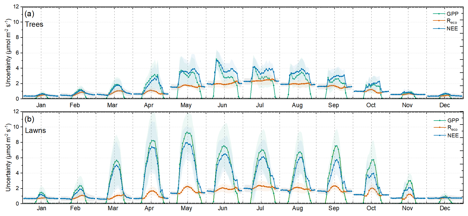
Figure 7 Monthly diurnal hourly averages (dots) and standard deviations (shading) of the estimated GPP, R_eco, and NEE uncertainties for (a) park trees and (b) lawns. The monthly averages consider the years 2022 and 2023 together.

3.5 Share of biogenic fluxes in the city

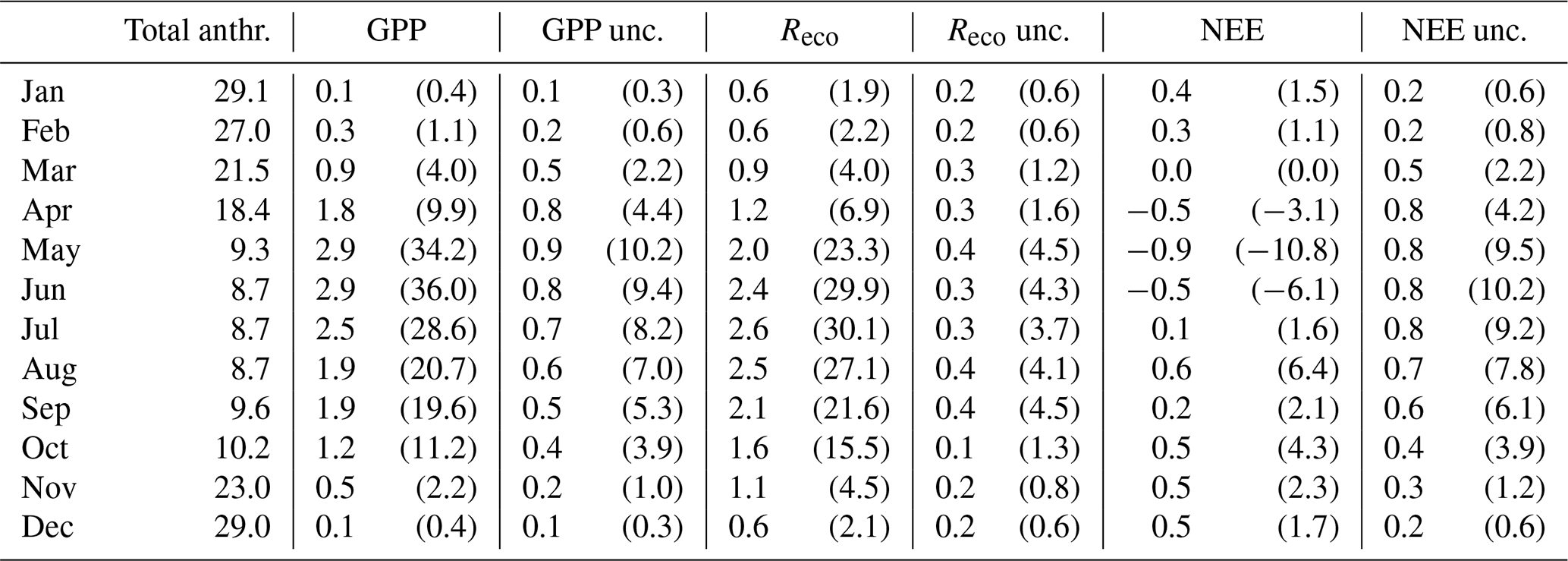
The comparison between the monthly biogenic fluxes and their uncertainties to the total anthropogenic emissions is presented in Table 3. It is evident that, during the winter, the biogenic fluxes and their uncertainties were insignificant compared to the anthropogenic emissions. However, during late spring, the anthropogenic emissions abruptly decreased due to the absence of building heating, and, at the same time, the biogenic components became more active. Therefore, GPP and R_eco are the competing processes, whose magnitudes reached 30 % to 36 % of the net monthly CO₂ balance when considered individually (Table 3). The contribution of NEE peaked during May, when both trees and lawns were in their optimal season, reaching −10.8 % of the monthly net budget. Even though the contribution was rather small on a monthly scale due to the trade-off between GPP and R_eco, its estimated uncertainty was similar to that of GPP (Table 3). It appears that the uncertainties associated with NEE can be an important part of the urban CO₂ cycle even in a city centre during summer and early autumn, as their magnitudes were found in this study to range between 6.1 %–10.2 % of the net monthly balance. It is important to note that the simple method of estimating the uncertainties of the biogenic flux components from the model spread may underestimate the real uncertainties, as the models partially rely on the same inputs and on similar assumptions. This is shown, for example, by the fact that the model spread does not always encompass the observed values of R_eco at the lawn locations.

Table 3 Monthly average fluxes ($\mathrm{\mu }\mathrm{mol}{\mathrm{CO}}_{\mathrm{2}}{\mathrm{m}}^{-\mathrm{2}}{\mathrm{s}}^{-\mathrm{1}}$) of the city's central 2 km × 2 km domain (Fig. 1), considering the total anthropogenic emissions (building heating, industry, vehicle traffic, human respiration) and the biogenic CO₂ flux components (GPP, R_eco, NEE) and uncertainties (unc., Sect. 3.3). The percentages (%) of the total monthly CO₂ balances are given in parentheses. The data are monthly averages of the years 2022 and 2023.

4 Discussion

4.1 Advantages and disadvantages of different types of biogenic CO₂ exchange models in urban contexts

Even though the models tested were forced with the same data, it is challenging to establish a clear hierarchy of model performance using the available measurements, as the performance of individual models seems to differ with different drivers or proxies for CO₂ exchange (Fig. 6). All tested models agreed on the timing of the spring recovery of trees in terms of GPP in 2022. However, at the beginning of the 2023 season, SUEWS, VPRM, and diFUME were again consistent among each other, but their GPP values started to grow earlier than the observed recovery in sap flow and in the LAI (Figs. 3a–b and B1a). JSBACH simulated an even earlier onset. On the other hand, the seasonal dynamics of JSBACH were found to be accurate in a recent study in hemiboreal tree-covered urban areas in Helsinki (Thölix et al., 2025), suggesting that the timing of spring recovery dynamics in JSBACH should be examined with longer and wider datasets in different ecosystem types. The overall evaluation of modelled tree GPP based on the sap flow dynamics indicates that all tested models provide reasonably accurate GPP estimates. The R_eco values for tree-covered areas by JSBACH, SUEWS, and VPRM were closer to each other than that of diFUME (Fig. 3c, d). Unfortunately, the autotrophic respiration of the aboveground tree parts is especially difficult to measure; therefore, the analysis is unable to reveal the best model regarding tree R_eco.

For lawns, JSBACH successfully estimated soil moisture and outperformed other models in predicting observed R_eco, which, on the other hand, exhibited much more variability than the simulations (Fig. 4c). Even though JSBACH simulated slightly higher diurnal variation in R_eco, the dynamics of the simple VPRM and the process-based ecosystem model JSBACH are comparable (Fig. 4c, d). Compared to VPRM and JSBACH, diFUME and SUEWS simulated higher and lower R_eco, respectively, and consistently lower GPP. Despite the dry periods in the summer months, VPRM and JSBACH also predicted similar annual cycles and day-to-day variability in GPP, but, unfortunately, direct measurements of lawn GPP were not available in this study. Nonetheless, GPP estimates by JSBACH for lawn have been tested and shown to be sufficient in hemiboreal zones using repeated measurements for photosynthesis (Trémeau et al., 2024). VPRM was evaluated in an urban forest and grassland area using field-based reference data by Winbourne et al. (2022), who found that R_eco was substantially overestimated during winter months but that the GPP was approximated with better accuracy. This is consistent with the present study, which shows higher R_eco values from VPRM compared to the other models in winter.

Overall, the four models are different in terms of sophistication and structure and in the fact that they use different data streams. Therefore, different advantages and disadvantages can be expected, depending on the application and context. All of the models require temperature and radiation inputs. However, VPRM requires the least number of data streams among the models (Table 2). diFUME and VPRM use satellite data to track vegetation phenology (Table A1), making them more suitable for monitoring purposes, especially in urban areas, where the vegetation type heterogeneity is so pronounced that it is very difficult to model accurately. As also demonstrated by the current study, these satellite-based models are able to detect changes in leaf area due to phenological shifts or stressful events, such as drought, providing valuable insights into ecosystem responses to environmental change. However, these models are not able to predict future carbon cycling under different climate scenarios or planning strategies, as they rely heavily on observations.

Despite the different levels of sophistication of the four models in simulating GPP, all consider some sort of hyperbolic function to model the response of gross photosynthesis to light and a bell-shaped dependence on air temperature (Table A1). On the other hand, the responses of photosynthesis to vapour pressure deficit and soil water availability are accounted for very differently in each model. VPRM uses a very simplistic approximation of drought effects on GPP based on LSWI, diFUME and SUEWS use empirical functions, and JSBACH has the most sophisticated approach to modelling drought effects (Sect. 2.3, Table A1). The generally good agreement between the models in simulated tree GPP seasonally and diurnally indicates that the simple process approximations were sufficient, possibly due to the lack of intense drought effects on tree GPP in this study based on the sap flow observations (Fig. 3a, b). On the other hand, drought effects on lawn GPP were captured by all models during August 2022, with VPRM showing the most intense drought-induced GPP reductions which were repeated in summer 2023 (Fig. 4a, b). These findings indicate that VPRM is very sensitive to LSWI and EVI indices (Fig. B1b, c), which can drive GPP to excessively low values during dry periods, in contrast to the process-based JSBACH and the empirical functions of diFUME and SUEWS. Unfortunately, we do not have any independent measurements of lawn GPP in this study to evaluate which type of model is closest to the truth.

Even though there are some similarities between the models in the representation of the GPP process, the description of R_eco significantly differs in terms of approximations and sophistication. JSBACH is the only model tested that includes carbon pools, which are essential for studying long-term temporal dynamics. This feature allows JSBACH to model the behaviour of soil carbon pools and their changes over extended periods. For instance, if high decomposition rates persist, the decreasing soil carbon pool also decreases heterotrophic emissions, whereas other models tested do not have such feedbacks and use only empirical environmental response functions. diFUME uses a more detailed approach compared to SUEWS and VPRM, separating above- and belowground respiration and using T_air, T_soil, SWC, and LAI as proxies, whereas SUEWS and VPRM use an exponential and a linear response function on T_air, respectively (Table A1). Despite the differences in the representation of R_eco, the seasonal and diurnal variabilities were not very different between the four models (Figs. 3c–d and 4c–d), and the differences detected were not clearly related to the level of sophistication but rather to the choice in parameterization. For example, diFUME tree R_eco was higher than the other models because the parameterization was kept the same for lawn and tree sites. JSBACH showed the best performance in predicting lawn R_eco (Fig. 6d), but, on the other hand, ecosystem process models such as JSBACH require very detailed input information (e.g. on soil carbon stocks) and are based on full-cycle assumptions that are difficult to meet in highly managed and disturbed urban ecosystems where carbon pools are constantly altered by human interventions (Golubiewski, 2006). Furthermore, process-based models such as JSBACH require a large number of input parameters compared to simple light use efficiency models such as VPRM, which has, in some cases, been found to outperform process-based models in explaining CO₂ variability (Gourdji et al., 2022).

It is important to highlight the limitations of the current study in terms of evaluating the models in the urban context. This study focuses on four urban parks where the effects of buildings and paved surfaces on energy and water exchange are not as pronounced as in urban canyons. Urban canyon vegetation and street trees in particular grow in a very different environment compared to urban parks (Dahlhausen et al., 2018; Nielsen et al., 2007), and their ecophysiological responses and dynamics can be potentially different from park trees. In this study, we apply SUEWS and diFUME, which are specifically designed for urban applications and include aspects of urban morphology in the simulations of biogenic CO₂ fluxes. Specifically, SUEWS stands out in assessing the urban energy balance and its effect on local air temperatures. This model is particularly advantageous in urban contexts where a detailed understanding of the energy exchanges is crucial for microclimate. A distinct feature of diFUME is that it has a 3D radiation module that takes into account building shading and diffuse radiation extinction within urban canyons. As the role of buildings, runoff, and local temperature is not as evident in the park applications of the current study, it is possible that the additional benefits of these models are not highlighted in the model intercomparison. In order to achieve a more thorough evaluation of the models and their applicability in the urban context, future research is needed, focusing on different urban environments, including vegetated street canyons.

4.2 In situ observations and challenges

Despite the technical, logistical, and methodological challenges in measuring sap flow and estimating tree transpiration in urban areas, such observations can be very valuable for monitoring tree physiological dynamics, especially in areas of extreme heterogeneity, where other techniques, such as eddy covariance, cannot be applied (Ewers and Oren, 2000; Peters et al., 2010). The sap flux densities measured in this study were very consistent with the seasonal and diurnal variability and magnitude for similar species, presented in other studies in suburban and urban areas (Bush et al., 2008; Peters et al., 2010; Rahman et al., 2017). Tilia sp. and Platanus sp. trees measured in this study, being semi-ring porous species (Schoch et al., 2004), present relatively constant maximum sap flux densities throughout the growing period due to the increased stomatal regulation (Bush et al., 2008; Peters et al., 2010). This suggests limited stomatal opening during high VPD and incoming radiation conditions, which also limit photosynthetic rates. Similarly to the results of the present study, measured sap flux densities in other studies responded only marginally to decreases in topsoil water content during summer (Peters et al., 2010; Rahman et al., 2017), indicating that the water availability in deeper soil layers is more important for maintaining the required hydraulic conductance of mature trees during summer. In the present study, we used a simple linear regression approach to derive reference daily tree GPP values from sap flow observations rather than a more sophisticated approach (e.g. Schäfer et al., 2003) to avoid involving a lot of modelling in our reference dataset. The disadvantage of the approach used is that it cannot predict the absolute magnitude of the GPP and only provides information about the daily variability.

Flux chamber R_soil and lawn R_eco observations serve as a direct reference for model evaluation, but they can greatly vary across different urban locations, and there are technical and logistical limitations in their application across urban spaces. For example, this study focused on large green areas in Zurich to obtain representative measurements of CO₂ flux behaviour of the park lawns under the city's management practices. These lawns are very busy public areas; therefore long-term installations (e.g. automated chambers) are not possible and the observations are limited to specific dates and times of field campaigns. The wealth of information that can be derived from continuous long-term automated chambers (e.g. Hill et al., 2021) cannot be compared to the sporadic field measurements. For example, the sudden increase in R_eco on the sunny lawn of Hardaupark in April 2023 would probably be easier to confirm and explain if we had continuous observations. Moreover, clear chamber measurements over park lawns were not implemented during this study but would be considered very helpful for estimating lawn NEE and partitioning to GPP and R_eco. Having this information during the field campaigns would be valuable for the complete evaluation of the model performance over lawns. Such measurements are currently implemented in the ICOS Cities project pilot case study sites of Paris and Munich, complementing the observations presented in this study.

The observations of R_soil and lawn R_eco presented in this study are comparable with what has been reported in the literature concerning urban park lawns. Even though it is well established that the main drivers of R_soil and R_eco are T_soil and water content (e.g. Raich and Schlesinger, 1992), the response functions and magnitudes of respiration in urban parks can be significantly different from native grasslands (Kaye et al., 2005). There are several studies that have measured soil organic carbon (SOC) pools across urban parks and natural ecosystems (e.g. Golubiewski, 2006; Kaye et al., 2005; Pouyat et al., 2006; Weissert et al., 2016). SOC pools vary across urban parks and are an important determinant for both R_soil and plant productivity (Golubiewski, 2006; Kaye et al., 2005). In general, studies suggest that the sequestration of soil C in parks dominated with grass increases linearly with park age (Lal and Augustin, 2012), reaching even higher biomass productivity and larger SOC pools than native grasslands (Golubiewski, 2006; Kaye et al., 2005; Pouyat et al., 2006; Weissert et al., 2016). However, this process can be severely affected by management practices, such as mowing, fertilization, and irrigation, which can also affect the balance between respiration and photosynthetic rates.

Allaire et al. (2008) compared respiration rates of urban turfgrass, measured with chambers under different fertilization and mowing treatments, and found that mowing frequency had a higher impact on respiration than fertilization and soil characteristics. Similarly to our observations, the lawn R_eco observed by Allaire et al. (2008) peaked suddenly in spring at the treatment with frequent mowing, reaching a maximum at around 14 $\mathrm{\mu }\mathrm{mol}{\mathrm{m}}^{-\mathrm{2}}{\mathrm{s}}^{-\mathrm{1}}$. Kaye et al. (2005) found consistently high R_soil and belowground C allocation in intensively mowed and irrigated urban lawns, 2.5 times higher than in adjacent native and agricultural ecosystems. It appears that mowing with return of clippings on the ground rapidly increases the R_eco under wet and warm conditions due to accelerated microbial activity. Furthermore, mowing alters the microenvironment of the lawn surface, leading to increased radiation exposure and temperatures of grass leaves, which can significantly alter leaf respiration rates (Shen et al., 2013). The R_eco observations in this study during the spring and summer of 2023 were probably affected by mowing, which increased R_eco to very high values in sunny areas, even higher than 20 $\mathrm{\mu }\mathrm{mol}{\mathrm{m}}^{-\mathrm{2}}{\mathrm{s}}^{-\mathrm{1}}$ in some cases. Detailed information on the management practices and their timing would be very valuable for interpreting the observations, but unfortunately it was not available. High values of maximum grass R_eco, similar to those in the present study and Allaire et al. (2008), were also reported by Liss et al. (2009) and Weissert et al. (2016) over park, residential, and sports field lawns under warm and moist conditions. However, the mowing effects were not clear in these studies.

4.3 Possibilities to mitigate climate change via urban C sequestration

Vegetation is able to sequester part of the anthropogenic emissions originating from fossil fuel burning. In this study, the vegetation uptake in central Zurich covered nearly 11 % of the total carbon budget in the optimal month of May. The summertime offset in this study is smaller than that observed in Helsinki (42 %; Havu et al., 2024), New York (20 %–40 %; Wei et al., 2022), and Florence (26 %; Vaccari et al., 2013), which is likely due to the fact that the studied area is highly built, with only 30 % vegetation. The forest-covered hills surrounding the city, for example, are not included in this area. As photosynthesis is minimal during the winter months, this results in a small offset of anthropogenic emissions on an annual scale. In central Helsinki, vegetation was found to take up 3 % of the anthropogenic emissions on an annual scale, whereas, at the scale of the whole city, the offset was 7 % (Havu et al., 2024; Järvi et al., 2019). Prior studies have reported annual offsets of 2.1 % in Boston (Hardiman et al., 2017) and 6.2 % in Florence (Vaccari et al., 2013), but, naturally, the offset is strongly dependent on the strength of anthropogenic emissions.

These numbers demonstrate the potential of urban vegetation to mitigate climate change. With the anthropogenic emissions potentially decreasing in the future, the contribution of biogenic fluxes will increase. It is also important to remember that the C sequestration of vegetation is highly dependent on its wellbeing; thus it is critical to find natural solutions that are resilient to heat, drought, and pests. Species diversity plays a crucial role here.

5 Conclusions

This study compared for the first time four different types of biosphere models (diFUME, JSBACH, SUEWS, VPRM) in terms of their accuracy in simulating CO₂ exchange (GPP, R_eco, NEE) in urban parks. Model simulations were evaluated against in situ observations in order to identify advantages and disadvantages of the different model types. The results showed a good agreement between all models in terms of magnitude and seasonality of park tree GPP, but there is potentially a challenge for process-based models (JSBACH, SUEWS) to accurately simulate the onset of tree greening in spring compared to remote-sensing-based models (diFUME, VPRM). On the other hand, there were larger differences between the R_eco simulations over both trees and lawns, as well as lawn GPP. However, in situ observations showed that all models underestimated the high lawn R_eco values in spring and summer, with the effects of grass mowing most likely being a factor that could not be captured by any model. The annual NEE estimates of the models agreed that, on average, park lawns acted as CO₂ sources and tree-covered park areas acted as CO₂ sinks during the simulation period, with the exception of diFUME, which simulated both trees and lawns as CO₂ sources. When compared to the anthropogenic CO₂ emissions, the simulated monthly NEE and its uncertainties were a considerable fraction of the net urban emissions during the vegetation growing period, reaching its maximum impact in late spring, with NEE being 10.8 % and its uncertainty being 10.2 % of the net CO₂ balance.

Overall, the results of this study do not provide a clear indication of the superiority of sophisticated process-based models, such as JSBACH, over simple light use efficiency models, such as VPRM, in simulating the dynamics of CO₂ fluxes in urban parks. However, this study is restricted to urban park vegetation, and the presented results cannot be easily generalized to other urban environments, such as vegetated urban canyons. Further research is needed to obtain a full understanding of the model applicability and efficiency across the wide heterogeneity of urban areas. The main limitation towards a more thorough model evaluation is the lack of urban in situ observations, mainly due to the technical, methodological, and logistical challenges of deriving representative observations across urban vegetation. More detailed, frequent, and spatially extended in situ observations would be necessary for a full assessment of model applicability. Specifically, grass chamber observations with clear and opaque chambers and even long-term continuous installations would be ideal to evaluate the model performance to simulate park lawn GPP, R_eco, and NEE. However, precautions must be taken in the design and implementations of such observations to avoid changing the microenvironment of the observation site and to allow the normal management procedures to be applied (e.g. mowing) so that the observation sites would still be representative of the park conditions. Regarding CO₂ exchange at tree scale, sap flow observations are a promising method to monitor tree physiological behaviour despite the application challenges. The extreme heterogeneity of tree species, age, and environmental conditions of the urban areas remains a huge challenge for urban model evaluation studies.

Appendix A: Model architecture and process representation

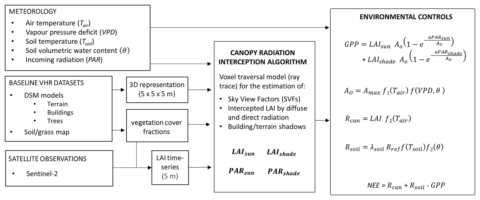
Figure A1 Process flow diagram of diFUME. A detailed description of the model can be found in Stagakis et al. (2023b).

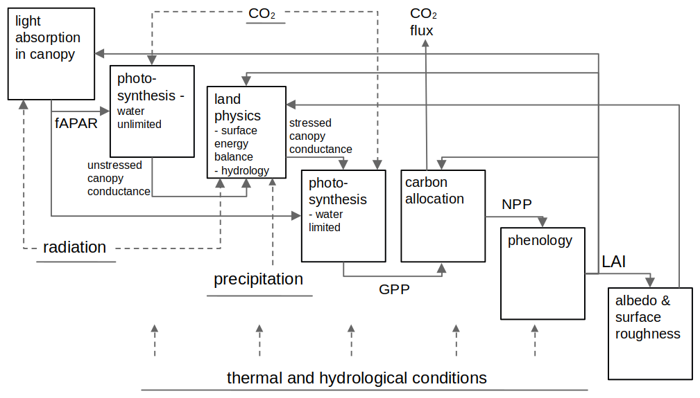
Figure A2 Process flow diagram of JSBACH. A detailed description of the model can be found in Reick et al. (2013).

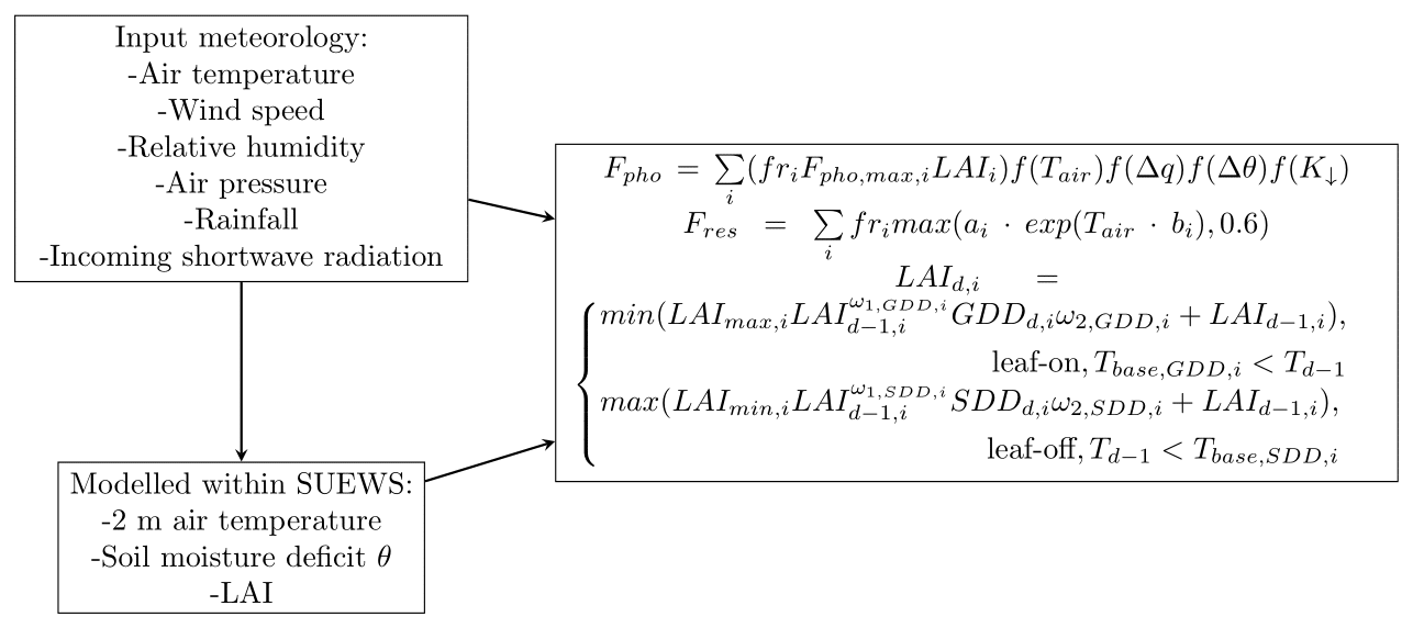
Figure A3 Process flow diagram of SUEWS. A detailed description of the model can be found in Järvi et al. (2011, 2019).

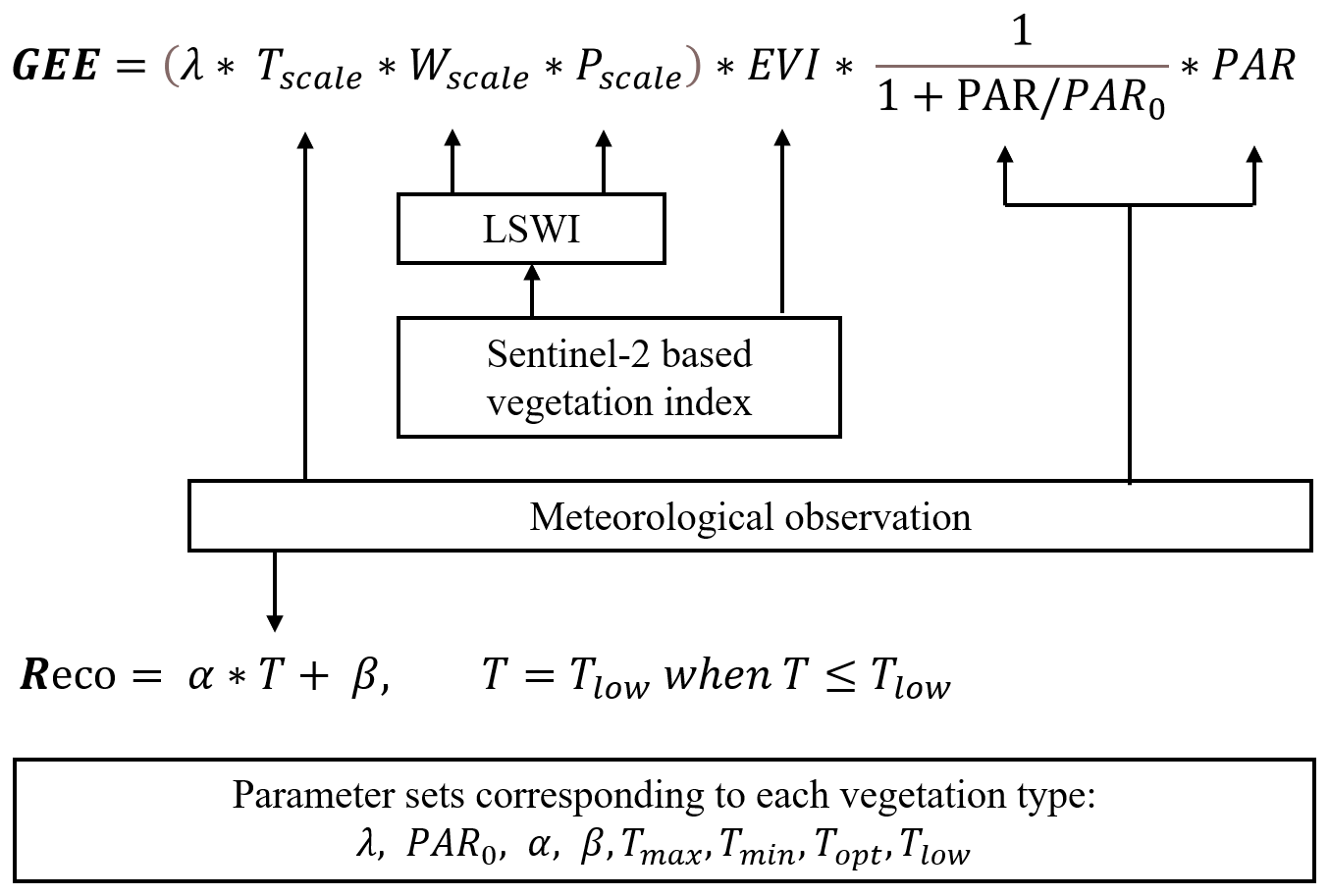
Figure A4 Process flow diagram of VPRM. A detailed description of the model can be found in Mahadevan et al. (2008).

Table A1 Overview of the main equations used by each model to estimate gross primary production (GPP), ecosystem respiration (R_eco), and phenology. The original notation of each model was preserved to facilitate the comparison with the relevant publications and the flow diagrams. The parameters of the equations are explained in the Supplement. The detailed descriptions of each model can be found in the respective references provided in Sect. 2.3.

Appendix B: Comparison between in situ observations and modelled parameters

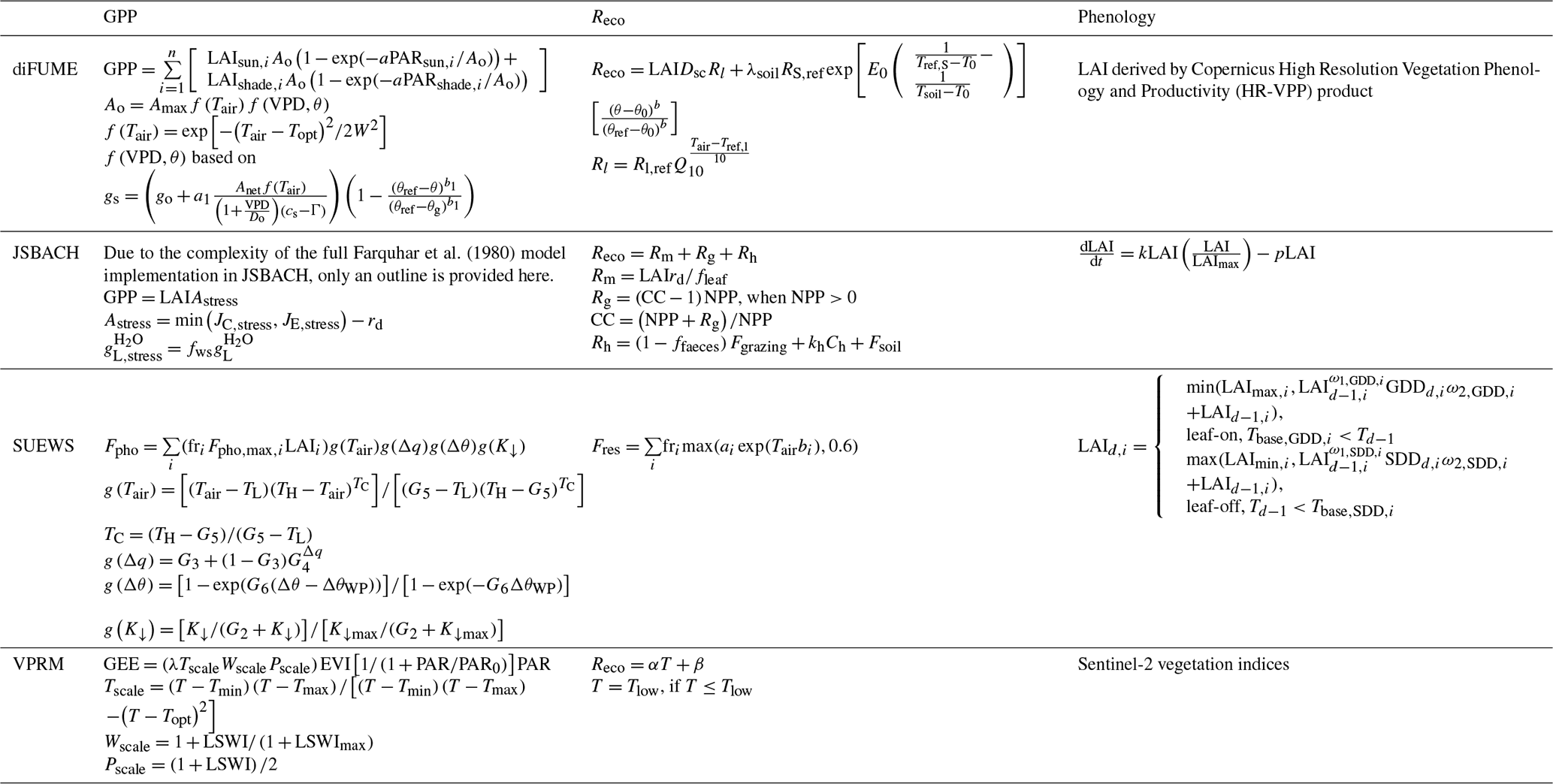
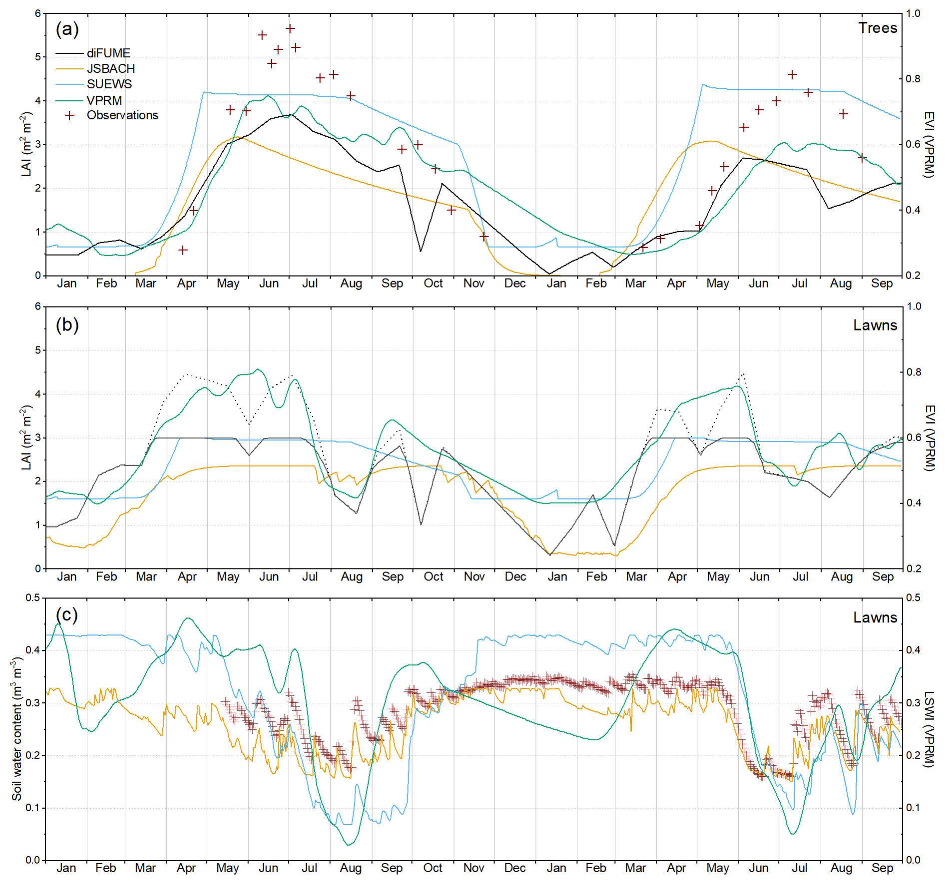
Figure B1 Time series of daily (a) modelled and observed tree leaf area index (LAI) by diFUME, JSBACH, and SUEWS together with EVI estimates by VPRM; (b) lawn LAI by diFUME, JSBACH, SUEWS, and VPRM lawn EVI; (c) observed and modelled soil water content in the lawns by diFUME, JSBACH, and SUEWS together with the Land Surface Water Index (LSWI) by VPRM. In panel (b), the dotted line shows the original diFUME LAI before the upper threshold of 3 m² m⁻². All datasets are averaged between the four parks, except tree LAI, where only Bullingerhof and Hardaupark are used.

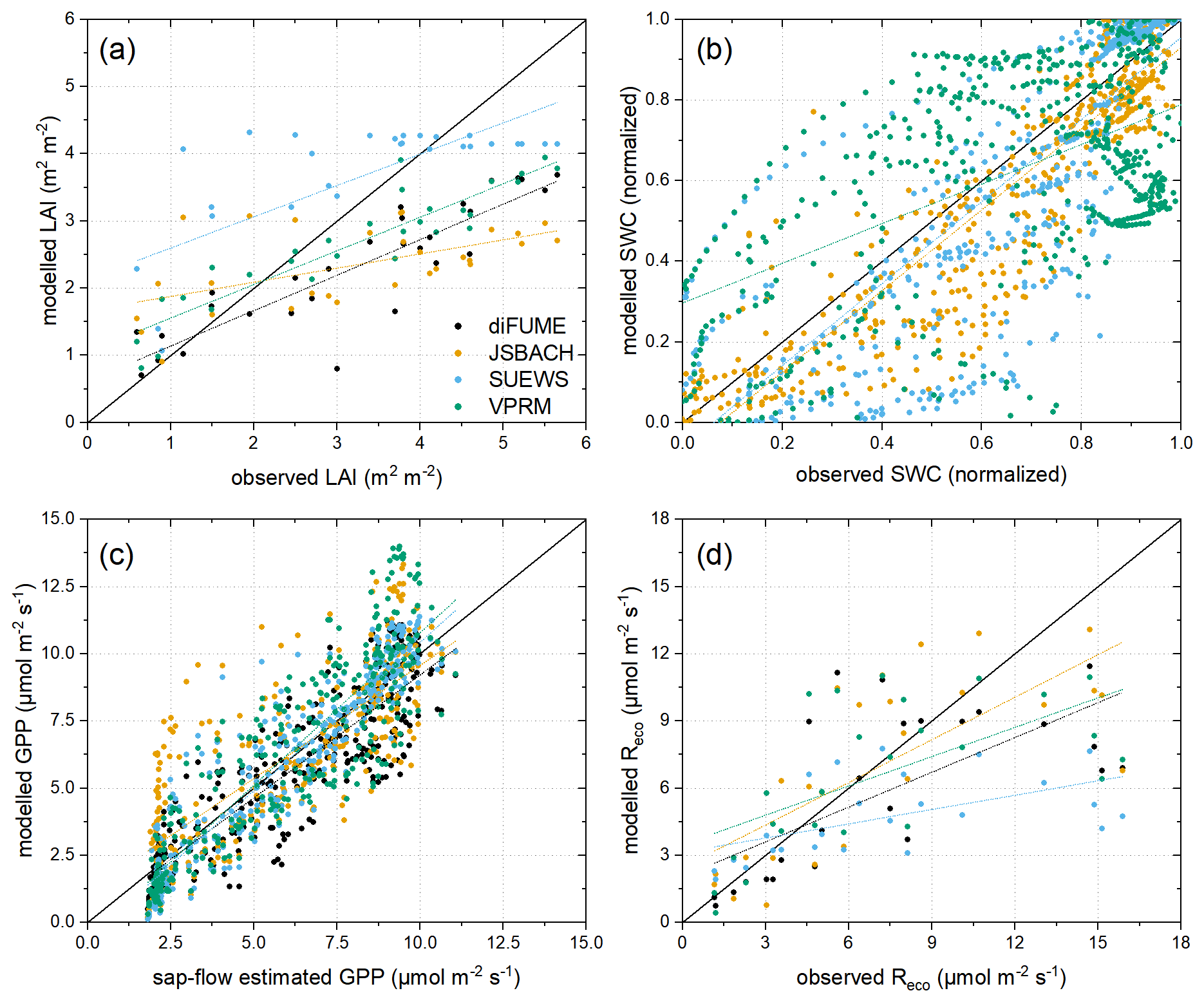
Figure B2 Scatterplots between (a) observed and modelled tree leaf area index (LAI), (b) normalized observed and modelled soil water content (SWC) of lawns, (c) observed and modelled tree gross primary production (GPP), and (d) observed and modelled lawn ecosystem respiration (R_eco). The 1:1 lines are thick black lines, and the linear fits for each model are presented with its respective colour. The evaluation metrics of the comparisons are presented in the Taylor diagram (Fig. 6). For the conversion of VPRM EVI to LAI, VPRM LSWI to SWC, and tree sap flow observations to tree GPP, see Sect. 2.5.