The distribution and abundance of planktonic foraminifera under summer sea ice in the Arctic Ocean

Planktonic foraminifera are calcifying protists that represent a minor but important part of the pelagic microzooplankton. They are found in all of Earth's ocean basins and are widely studied in sediment records to reconstruct climatic and environmental changes throughout geological time. The Arctic Ocean is currently being transformed in response to modern climate change; however, the effect on planktonic foraminiferal populations is virtually unknown. Here, we provide the first systematic sampling of planktonic foraminifera communities in the “high” Arctic Ocean – defined in this work as areas north of 80° N – specifically in the broad region located between northern Greenland (the Lincoln Sea with its adjoining fjords and the Morris Jesup Rise), the Yermak Plateau, and the North Pole. Stratified depth tows down to 1000 m using a multinet were performed to reveal the species composition and spatial variability in these communities below the summer sea ice. The average abundance in the top 200 m ranged between 15 and 65 individuals m⁻³ in the central Arctic Ocean and was <0.3 individuals m⁻³ in the shelf area of the Lincoln Sea. At all stations, except one site at the Yermak Plateau, assemblages consisted solely of the polar specialist Neogloboquadrina pachyderma. It predominated in the top 100 m, where it was likely feeding on phytoplankton below the ice. Near the Yermak Plateau, at the outer edge of the pack ice, rare specimens of Turborotalita quinqueloba occurred that appeared to be associated with the inflowing Atlantic Water layer. Our results would suggest that the anticipated turnover from polar to subpolar planktonic species in the perennially ice-covered part of the central Arctic Ocean has not yet occurred, in agreement with a recent meta-analysis from the Fram Strait which suggested that the increased export of sea ice is blocking the influx of Atlantic-sourced species. The presented data set will be a valuable reference for continued monitoring of the abundance and composition of planktonic foraminifera communities as they respond to the ongoing sea-ice decline and the “Atlantification” of the Arctic Ocean basin. Additionally, the results can be used to assist paleoceanographic interpretations, based on sedimented foraminifera assemblages.

1 Introduction

Planktonic foraminifera are unicellular protists that form an important component of the pelagic biome. Their calcareous tests are common in the sediment record and are widely used as tracers of climatic and oceanographic conditions throughout geological time (Schiebel and Hemleben, 2017). To understand the response of foraminiferal communities to climatic change, a thorough understanding of their ecology is required. This is crucial for correctly interpreting temporal and spatial variations in foraminiferal assemblages and their geochemical signatures. One region that is vastly understudied with respect to its planktonic foraminifera is the high Arctic Ocean (defined here as the ocean areas north of 80° N). With sea ice retreating rapidly (Meier and Stroeve, 2022) and Atlantic waters increasingly influencing the Arctic domain (a process dubbed “Atlantification”; Polyakov et al., 2017), pelagic ecosystems are expected to be significantly affected (Brandt et al., 2023). While the footprint of these processes on planktonic foraminifera communities is presently unknown, a recent meta-analysis suggests that the increased export of sea ice through the Fram Strait is currently playing a key role in blocking the flux of subpolar planktonic foraminifera towards the high Arctic Ocean (Greco et al., 2022). It is anticipated that once this export ceases (i.e., essentially when the Arctic Ocean becomes seasonally ice-free), subpolar species will be able to rapidly invade the high Arctic Ocean (Greco et al., 2022).

Baseline information and the monitoring of planktonic foraminifera are needed to assess the impacts of the unfolding changes, especially in the sea-ice-dominated high Arctic Ocean. Nevertheless, knowledge of resident pelagic communities in the remote, perennially ice-covered regions is minimal. Thus far, most studies have documented living planktonic foraminifera from the Arctic region stemming from areas within or near the seasonal sea-ice zone or close to sea ice that is exported through the Fram Strait (Carstens et al., 1997; Darling et al., 2004; Pados and Spielhagen, 2014; Volkmann, 2000). These studies show that Neogloboquadrina pachyderma and Turborotalita quinqueloba are the dominant species in these regions, with occasional traces of Globigerinita uvula and Globigerinita glutinata. Only two previous studies have reached sites located far into the perennial ice pack; this includes sampling stations at the Alpha Ridge at ca. 83° N (Bé, 1960) and stations up to 86° N in the Nansen Basin (Carstens and Wefer, 1992). Bé (1960) observed assemblages consisting solely of N. pachyderma, at abundances ranging from 0 to 2.4 individuals m⁻³ at depths down to 500 m (single net). However, due to the large mesh size of the sampling net (200 µm) used in Bé (1960), the results are not directly comparable to more recent work, which emphasizes the need for small net mesh sizes in the Arctic Ocean. Ideally, a 63 µm mesh is used to sample juvenile N. pachyderma and small subpolar species, such as T. quinqueloba and G. uvula. This is important because T. quinqueloba individuals are particularly small in the Arctic region (Kandiano and Bauch, 2002) and, thus, could be missed without the correct sampling approach. Exploring the environmental factors that limit the modern presence of T. quinqueloba in the central Arctic Ocean is a relevant topic (Vermassen et al., 2023). Two earlier plankton tow transects crossing the Nansen Basin found that T. quinqueloba decreased from ca. 30 % of the standing stock at 81° N to 2 %–15 % at 86° N (Carstens and Wefer, 1992). It was suggested that these individuals may have been advected in the Atlantic Water flow path, via branches of the West Spitsbergen Current that delivers Atlantic Water to the central Arctic Ocean. Carstens and Wefer (1992) also proposed that the area of reproduction of this species was located further south.

Here, we report the assemblage composition and depth distribution of planktonic foraminifera from eight vertical multinet hauls conducted in ice-covered waters in the high Arctic Ocean in late summer 2021 (SAS ODEN21). This is supplemented with 10 plankton hauls performed in the Lincoln Sea and adjoining fjords (Petermann Fjord and Sherard Osborn Fjord), conducted in late summer of 2019 (RYDER19). The aim of our study was threefold. First, we aimed to provide a snapshot of the standing stock of planktonic foraminifera underneath the perennial ice cover (summer sea ice; Figs. 1 and 2) and test whether subpolar species such as T. quinqueloba were present. Second, we investigated the relationship between ambient environmental conditions and the observed planktonic foraminifera distribution patterns in order to gain a better understanding of the factors that control planktonic foraminifera abundance and species composition. Third, we used an automated approach to extract and analyze morphometric data and explored whether these data could reveal clues regarding the population dynamics and, perhaps, the life history of N. pachyderma.

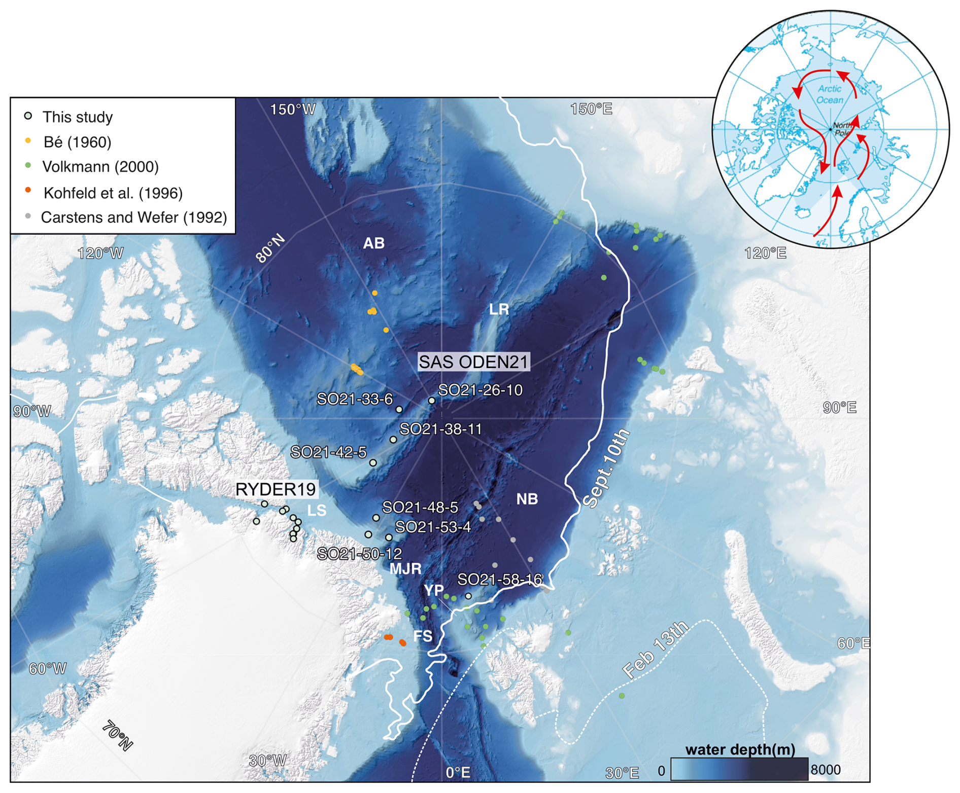
Figure 1 Bathymetric map of the Arctic Ocean (Jakobsson et al., 2020c) with sampling stations obtained during the SAS ODEN21 and RYDER19 expeditions (this study) and previous foraminifera sampling sites located north of 80° N. Full station names and coordinates of sampling sites are listed in Table 1. The abbreviations used in this figure are as follows: AB – Amerasian Basin; LR – Lomonosov Ridge; MJR – Morris Jesup Rise; YP – Yermak Plateau; FS – Fram Strait; LS – Lincoln Sea; and NB – Nansen Basin. The inset (upper right) shows the track of warm Atlantic waters (red arrows) into the central Arctic Ocean, as they subduct under cooler and fresher waters. Atlantic Water can enter the central Arctic Ocean through the Fram Strait or via the Barents Sea. The sea-ice extent on 13 February and 10 September in 2021 is also indicated (data from the US National Ice Center).

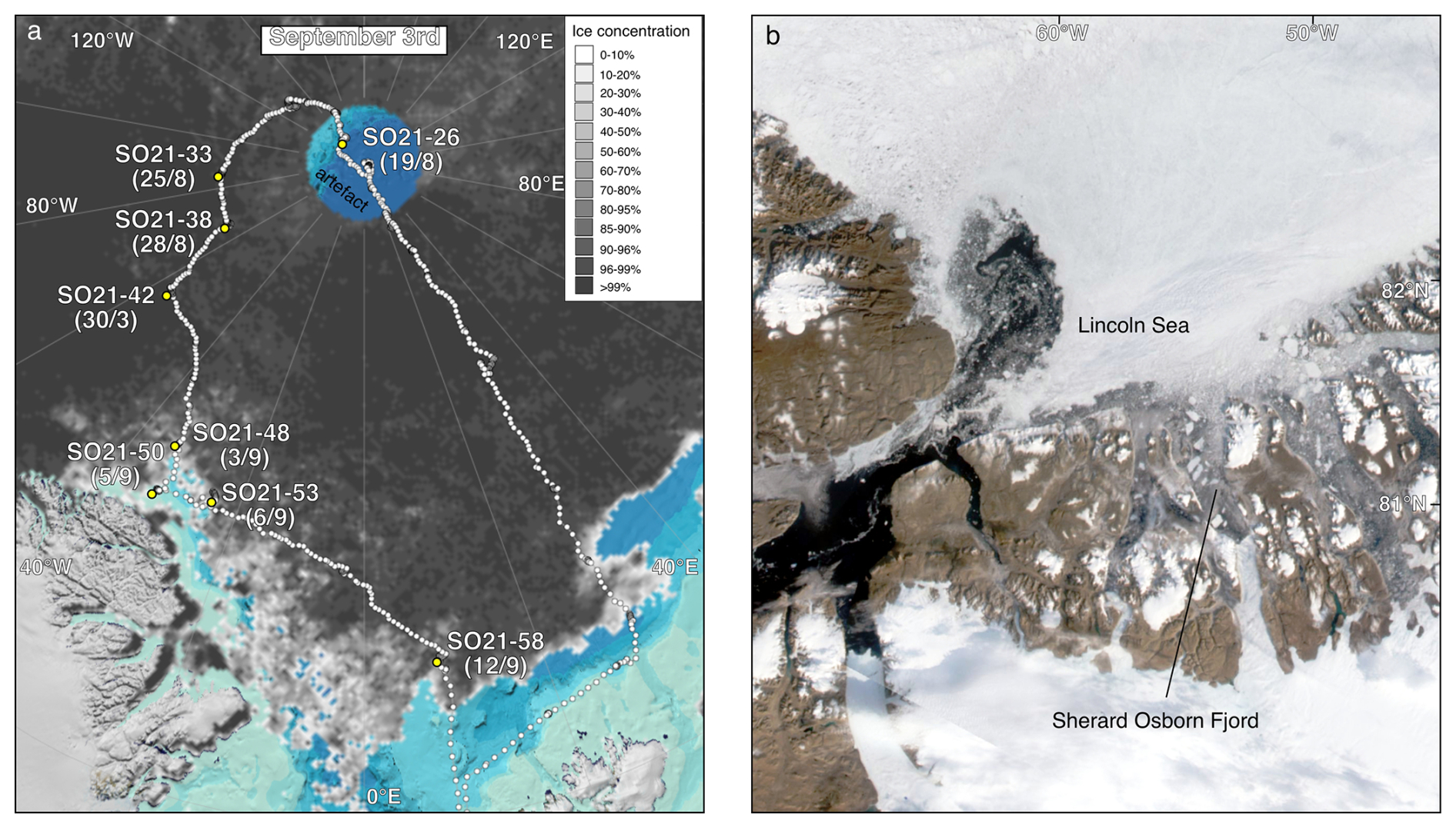
Figure 2 (a) Map displaying sea-ice conditions during the SAS ODEN21 expedition (cruise track indicated using white dots) on 3 September 2021 and the multinet sampling stations (yellow circles). Sampling dates are indicated in parentheses. Station names are abbreviated; the full station names are given in the caption of Fig. 1. Sea-ice data are from the University of Bremen, visualized using https://oden.geo.su.se/map/ (last access: 1 January 2023​​​​​​​). (b) A MODIS satellite image (3 September 2019) displaying general ice conditions during the RYDER19 expedition. Thick, multiyear sea ice covered most of the Lincoln Sea, whereas open water (with icebergs) was present in the fjords of North Greenland.

2 Methods

2.1 Sampling strategy

This study is based on two sampling campaigns conducted in the Arctic Ocean with the icebreaker (IB) Oden: the Synoptic Arctic Survey 2021 expedition (hereafter SAS ODEN21) and the Ryder 2019 expedition (hereafter RYDER19). Multinet sampling was conducted during SAS ODEN21 (Snoeijs-Leijonmalm, 2022), whereas single-net plankton hauls were conducted during RYDER19 (Jakobsson et al., 2020a). During SAS ODEN21, multinet water column sampling was conducted at eight stations from 19 August to 11 September 2021 at various times during the day under continuous-daylight (midnight sun) conditions (Table 1). Sample sites include the central Lomonosov Ridge (located 100 km south of the North Pole), the Makarov Basin, the southern Lomonosov Ridge, the area north of Greenland (Morris Jesup Rise), and the Yermak Plateau (Fig. 1). A multinet (Hydro-Bios Multi Plankton Sampler MultiNet^®, Type Midi) with a surface area of 0.25 m² was used. The net mesh was 55 µm, and the mesh of the sampling cup was 50 µm. Net clogging was not an issue in the ice-covered Arctic Ocean, where productivity and plankton standing stocks are relatively low compared to other ocean regions.

Table 1 Net sampling stations during SAS ODEN21 and RYDER19.

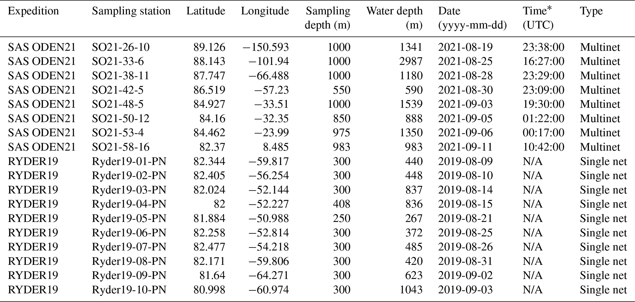
^* N/A: not available.

At each station, the bow of the ship was parked in the ice and plankton nets were deployed from the aft deck, i.e., in areas where the ice had been broken up by the ship. The area where the cable and net entered the water was kept free of incoming ice using water cannons located near the edge of the aft deck – these sprayed the ocean surface and created a small current away from the ship. Larger pieces of incoming ice were manually diverted using large boat hooks to push away incoming ice.

By default, the multinet was lowered to and hauled from 1000 m depth unless the site was shallower, in which case the multinet was hauled from ca. 20 m above the seafloor (Table 1). The default sampling depth intervals were 1000–500, 500–200, 200–100, 100–50, and 50–0 m. The upwards towing speed was 0.5 m s⁻¹, and towing was paused for approximately 1 min at the start of each sampling interval. After deployment, the samples were transferred from the sampling cups to containers. Samples were then pipetted onto a glass Petri dish and visualized under a microscope (ZEISS Stemi 508). Planktonic foraminifera individuals were picked onto microfossil slides using a combination of pipettes and brushes. Due to the number of individuals, multiple slides were commonly needed per depth interval for each site. Samples that could not be picked aboard the ship due to time constraints were preserved in an EtOH solution and picked post-cruise at Stockholm University. All planktonic foraminifera individuals were identified and counted. A systematic counting of cytoplasm content was performed at one station (SO21-26-10), but this was not possible at other sites due to time constraints. Throughout the study, we assumed that cytoplasm-bearing individuals were alive (i.e., “living”) and that the empty tests represented dead individuals that were sinking. However, recently deceased individuals may still have cytoplasm, and planktonic foraminifera can exhibit dormancy (Murray and Bowser, 2000; Ross and Hallock, 2016; Westgård et al., 2023). The abundance of planktonic foraminifera (number of individuals per cubic meter of filtered water) was calculated via the following formula:

$$\begin{array}{}\text{(1)}& {\displaystyle \frac{n}{a\cdot d}},\end{array}$$

where n represents number of individuals counted for a given depth interval, a is the surface area of the net, and d is the length of the sampled depth interval. The reported abundances include all tests, regardless of cytoplasm content.

A smaller-scale sampling program involving more opportunistic sampling was conducted during RYDER19 in the period from 9 August to 3 September 2019 (Table 1; Jakobsson et al., 2020a). A simple plankton net (60 cm diameter net opening, 83 µm mesh), with a 13 kg weight attached, was lowered to a depth of 300 m and hauled vertically at a rate of ca. 0.2 m s⁻¹, sampling the entire depth interval at 10 stations. On deck, the net content was washed out of the sampling cup with filtered seawater into a storage container, and planktonic foraminifera were then picked from the concentrate. For comparison with our data, abundances of N. pachyderma in the Nansen Basin reported by Carstens and Wefer (1992) were calculated by multiplying their reported percentage of N. pachyderma by their reported numbers of total planktonic foraminifera abundance. The abundance values of N. pachyderma in the top 200 m of other studies were calculated from the original data available online.

2.2 Test size and morphometric analysis

Picked individuals (N=15 381) were imaged with a Leica M205 C microscope. Tests were commonly divided over several slides (per depth interval, per site). On the slides, tests were organized on a series of squares, and one photo was taken for each square on the microfossil slides. Individuals were segmented from these images using the “segment” module of AutoMorph (Hsiang et al., 2017; development version available at https://www.github.com/ahsiang/AutoMorph, last access: 1 January 2023), which automatically separates and extracts individual imaged objects using traditional image-processing methods. As the lighting conditions were set manually and could change between images, all images were initially processed under “Sample” mode in AutoMorph to determine the optimal parameters (i.e., threshold value and minimum/maximum size of legitimate objects) for segmenting objects in each image. Threshold values tested ranged from 0.10 to 0.79 and size ranged from 50 to 500 µm, depending on the individual image conditions. Optimal parameter values were chosen to maximize the number of individuals correctly identified. A pixel size of 2.571 µm was used for both the x and y axes based on output from the Leica microscope. The images were then processed under “Final” mode with the optimal parameter values using batch-processing mode to obtain individual cropped images of each specimen. Incorrectly identified non-foraminifer material (e.g., organic fluff and junk images of the background texture of the slides) were removed manually in post-processing. All specimen images were compiled and then processed using the “run2dmorph” module of AutoMorph. This module detects the outlines of individuals and then automatically extracts morphometric measurements such as major/minor axis length, perimeter length, and area. Default values were used for all input parameters in run2dmorph.

2.3 CTD, chlorophyll a, and nutrients

Conductivity–temperature–depth (CTD) measurements for SAS ODEN21 were obtained using two standard Sea-Bird SBE911plus systems, one “shallow” (maximum 1000 m depth) and one “deep” (full-depth), each with dual sensors to measure temperature and salinity and single sensors to measure pressure and the dissolved oxygen concentration. For more information about hydrographic operations, we refer to the cruise report provided by Snoeijs-Leijonmalm (2022). Pre- and post-cruise, all sensors were calibrated by the Swedish Polar Research Secretariat. Salinity and oxygen were further calibrated against samples collected from the Niskin bottles of the rosette water sampler. Salinity samples from the deep stations were analyzed post-cruise using a Guildline Autosal salinometer and IAPSO (International Association for the Physical Sciences of the Oceans) standard seawater at GEOMAR, Germany. Dissolved oxygen was determined aboard the ship using an automatic Winkler titration setup with UV detection (Scripps Institute of Oceanography Oxygen Titration System version 2.35m). The fully calibrated data sets are freely available from the PANGAEA database (Heuzé et al., 2022a, b).

CTD measurements during the RYDER19 expedition were made with a Sea-Bird SBE911plus with dual temperature (SBE 3) and conductivity (SBE 04C) sensors. The CTD was equipped with a dissolved oxygen sensor (SBE 43), turbidity sensor (WET Labs ECO), fluorescence sensor (WET Labs ECO-AFL/FL), and altimeter (BENTHOS altimeter PSA-916D). The CTD was mounted on a 24-Niskin-bottle (12 L) rosette. All sensors were calibrated by the Swedish Polar Research Secretariat pre- and post-cruise. The data set is available from the Bolin Centre Database (Stranne et al., 2020) (Oceanographic CTD data from the Ryder 2019 expedition.)

On the SAS ODEN21 expedition, seawater was collected using an SBE rosette system equipped with 22 Niskin bottles (12 L), which was deployed from the bow of the ship. The bottles were closed at predefined depths (10, 20, 30, 40, 50, 75, 100, 125, 150, 200, 250, 300, 400, 500, 700, and 1000 m, following the international SAS protocol) during the return of the CTD from the bottom. Directly after the CTD was back on deck, water samples (100 mL) were taken from each Niskin bottle using clean sampling methods. As soon as possible after sampling, typically on the same day, concentrations of the macronutrients phosphate, nitrate + nitrite, ammonium, and silicate (PO₄, NO₃+NO₂, NH₄, and SiO₄) were determined colorimetrically on board using a four-channel continuous-flow analyzer with photometric detection (QuAAtro39, SEAL Analytical) on unfiltered seawater. The instrument was set up to use QuAAtro method nos. Q-064-05 Rev. 8, Q-119-11 Rev. 2, Q-069-05 Rev. 8, and Q-066-05 Rev. 5 for PO₄, NO₃+NO₂, NH₄, and SiO₄, respectively. These methods largely correspond to standard methods SS-EN ISO 15681-2:2018, SS-EN ISO 13395:1996, SS-EN ISO 11732:2005, and SS-EN ISO 16264:2004. Each analysis run included standards freshly prepared from stock solutions, certified reference material (VKI QC SW4.1B and VKI QC SW4.2B), and solutions for automatic baseline/drift correction.

Chlorophyll a was sampled at the defined depths down to 500 m. Samples were kept in 4.7 L brown bottles at low (∼ 4 °C) temperatures until processing. Size-fractionated samples were attained using 2.0 µm polycarbonate filters (diameter 25 mm) as well as 0.3 µm glass fiber filters (ADVANTEC^®, diameter 25 mm). Filters were placed inside Swinnex capsules and serially connected at the end of a peristaltic-pump system. Seawater was divided into two 2 L bottles to collect replicate samples and was pumped through the system at a low pump rate (30 rpm) to ensure cell integrity on the filters. Seawater was filtered either until the filter system clogged or 2 L of seawater passed through. Filters were immediately placed in test tubes with 2.5 mL 95 % EtOH and stored in the dark at room temperature for >16 h before measurement on a Trilogy fluorometer (Turner, USA). The instrument was calibrated using a standard from Anacystis nidulans (Sigma-Aldrich).

2.4 Statistical analysis

Statistical analyses were performed using Python (version 3.8.1). The statsmodels (version 0.11.1) and scikit-learn (version 0.23.1) libraries were employed to explore the data using generalized linear models (GLMs). The input variables included temperature, salinity, chlorophyll concentration, and distance to the sea-ice edge, with values averaged according to the respective depth intervals (N=24). The response variable was the foraminifera abundance. Data from the top three depth intervals (0–50, 50–100, and 100–200 m) were used, as nearly all living (cytoplasm-bearing) individuals were found at those depths. Given that the data were continuous and positively skewed, a gamma distribution with a log link were applied in the GLM. Predictor variables were standardized prior to the analysis. Multicollinearity was evaluated using the variance inflation factor (VIF). All variables exhibited VIF values below 5, indicating that multicollinearity was not a concern.

3 Results

3.1 Environmental conditions

3.1.1 Oceanography

As expected, three distinct water masses were present in the upper 1000 m analyzed here (e.g., Rabe et al., 2021; Rudels, 2000). In the top 10–150 m, a cold (ca. −1.5 °C) and low-salinity (29–34 g kg⁻¹) water mass was present (Figs. 3 and 4). This layer is commonly referred to as the Polar Surface Water (PSW), defined as σ_θ<27.7 kg m⁻³ (Rudels et al., 2008). Below this, a 500–800 m thick water mass occurred – the Atlantic Water – which is characterized by higher temperatures (>0 °C) and relatively high salinity (>34.9 g kg⁻¹). This water mass is derived from North Atlantic currents, which subside beneath the cold polar waters as they enter the ice-covered central Arctic Ocean. At station SO21-26-10, in the North Pole area, the Atlantic Water layer was markedly warmer (T_max=1.48 °C) than at the other sites on the Lomonosov Ridge and Morris Jesup Rise, implying a more proximal branch of inflowing Atlantic waters (Figs. 3 and 4). At station SO21-58-16, the PSW was much thinner and Atlantic-derived waters (T_max=1.64 °C) were present between 100 and 750 m depth (Fig. 4). Below the Atlantic Water, the deep water was characterized by temperatures lower than 0 °C, although with a salinity that remained high.

Similar hydrographic conditions were generally found in the area north of Greenland. In the Sherard Osborn Fjord, however, the shallowest 10 m of the PSW was “dammed” by the heavy sea-ice conditions outside the fjord, in the Lincoln Sea, which led to highly elevated temperatures (reaching 4 °C) low salinities (<15 g kg⁻¹), and low associated chlorophyll-a concentrations within the fjord (Figs. A1 and A2; Stranne et al., 2021). The Atlantic Water in the North Greenland fjords is, to some extent, influenced by subglacial runoff and melting from marine-terminating glaciers forming glacially modified water. This was particularly evident inside the Sherard Osborn Fjord, where local bathymetry influences the deep-water circulation inside the fjord (Jakobsson et al., 2020b; Nilsson et al., 2023; Figs. A1 and A2).

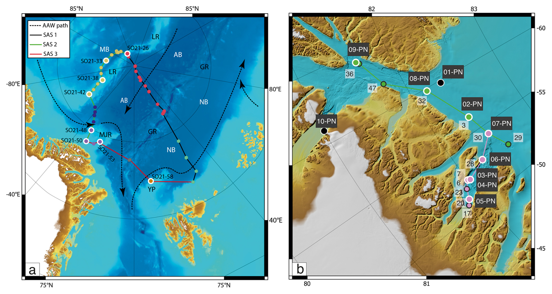
Figure 3 (a) Map showing the locations of CTD stations during SAS ODEN21 and the transects depicted in Fig. 4. Sites with white circles depict combined CTD and foraminifera sampling. (b) Map showing the locations of foraminifer sampling stations (white text on black labels: “xx-PN”) and CTD stations (black text on white labels) during RYDER19 and the transects depicted in Fig. 4. Sites with white circles depict combined CTD and foraminifera sampling sites. Arrows depict the circulation of Atlantic Water.

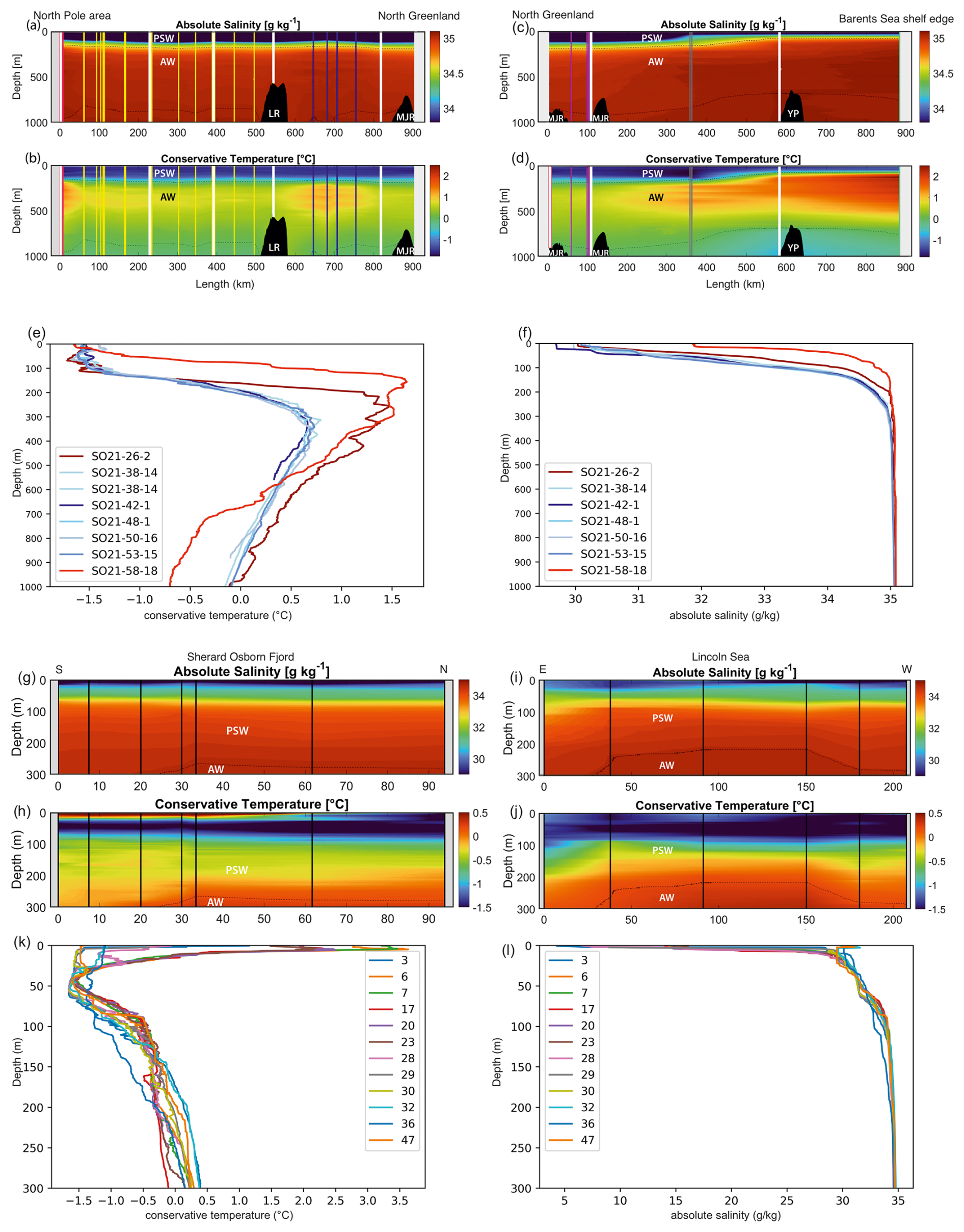
Figure 4 Oceanographic data (temperature and salinity) obtained during SAS ODEN21 (a–f) and RYDER19 (g–l). Transects of temperature (b, d, h, j) and salinity (a, c, g, i) are presented. Temperature profiles (e, k) and salinity profiles (k, l) combined for each expedition are also presented. Temperature and salinity profiles are shown for both the Lincoln Sea region and Sherard Osborn Fjord in Figs. A1 and A2, respectively.

3.1.2 Sea ice

All of the stations sampled during SAS ODEN21 were characterized by intense sea–ice conditions (ice coverage >95 %) (Fig. 2). Sea-ice thickness estimates derived from ice cores obtained near the sampling stations ranged from 1.1 to 2.6 m (average of 1.8 m; Snoeijs-Leijonmalm, 2022). However, these observations exhibit a bias towards a greater ice thickness, as sites with thicker ice were selected for safety and ship stability reasons. Therefore, the true regional average ice thickness reported here should be considered significantly lower.

Another factor that has a possible effect on planktonic foraminifera abundance is the distance to the sea-ice edge. For SAS ODEN21, stations SO21-26-10, SO21-33-6, SO21-38-11, and SO21-42-5 were located well within in the Arctic ice pack, >300 km from the nearest sea-ice edge, while stations SO21-50-12, SO21-53-4, and SO21-58-16 were located rather close to the ice edge (<50 km). Although station SO21-48-5 was located relatively close to a narrow lead of open water, it was located about 80 km from the broader sea-ice edge/marginal ice zone (Fig. 2).

In the Lincoln Sea, the ice cover generally consisted of multiyear sea ice that was several meters thick, but areas bordering North Greenland and off Ellesmere Island were temporarily ice-free (Fig. 2). Sherard Osborn was free of sea ice during the time of sampling, although icebergs were present.

3.1.3 Patterns of chlorophyll, nutrient, and oxygen concentrations

Concentrations of chlorophyll a were typically moderately high near the surface, increased with depth, and reached a maximum between 20 and 40 m water depth (Fig. 5). Maximum chlorophyll-a values ranged between 0.11 and 1.10 µg L⁻¹. Below this, concentrations decreased, until they became negligible at about 50–70 m depth. At station SO21-58-16, no distinct subsurface chlorophyll-a maximum was observed; instead, values at this station were highest near the surface (top 10 m).

Concentrations of nitrate + nitrite (NO₂ + NO₃), phosphate (PO₄), and silicate (SiO₄) displayed comparable depth profiles overall, although there were some differences among stations in the top 200 m. From the surface and down to the chlorophyll-a maximum, nutrients were strongly depleted, especially of NO₂ + NO₃ (Fig. 5). Between 50 and 150 m, a pronounced nutrient peak occurred at stations SO21-33 to SO21-53, typically with a maximum at around 75 m depth. This peak was much weaker at station SO21-26, where PO₄ and SiO₄ instead showed a minimum at around 100 m. At the Yermak Plateau (station SO21-58-16), there was no subsurface maximum; rather, there was a steep increase in nutrient concentrations down to 100 m. At greater depths, below 200 m, nutrient concentrations at all stations converged to very similar values.

Stations SO21-33 to SO21-53 shared similar trends with respect to the oxygen concentration throughout the water column (Fig. 5). In the top 30 to 50 m at these stations, oxygen values stayed broadly constant at around 8.9 mL L⁻¹. Down to 100 m, values decreased rapidly and remained constant at around 7.8 mL L⁻¹. At station SO21-26, values declined from 8.7 mL L⁻¹ near the surface to 6.9 mL L⁻¹ at 100 m, peaked to 7.6 mL L⁻¹ between 100 and 120 m, and then remained constant at 6.9 mL L⁻¹ below 120 m. At station SO21-58, oxygen values declined from 8.6 near the surface to 6.9 mL L⁻¹ at 100 m, below which they remained constant.

The nutrient and oxygen profiles (Fig. 5), as well as the salinity profiles (Fig. 5), indicate the presence of the Transpolar Drift Stream at stations SO21-33 to SO21-53, whereas surface waters near the North Pole (station SO21-26) and particularly on the Yermak Plateau (station SO21-58) were less influenced by this major ocean current in 2021.

3.2 Planktonic foraminifera

3.2.1 Regional variability

The variability in the average planktonic foraminifera abundance in the top 200 m was relatively high and ranged between 18 and 65 individuals m⁻³ at sites located in the central Arctic Ocean (SAS ODEN21; Fig. 6). No obvious spatial trends in abundance were observed in the central Arctic Ocean data set. The abundance of individuals in the water column appeared to be relatively low in the North Pole area (18 individuals m⁻³; station SO21-16-10) and close to the North Greenland coast (19 individuals m⁻³; SO21-50-12, ca. 60 km north of Cape Morris Jesup). The highest abundances occurred at the southern end of the Lomonosov Ridge (Greenland side) and the northern tip of the Morris Jesup Rise (58 and 65 individuals m⁻³ at SO21-42-5 and SO21-48-5, respectively; Fig. 6). In the Lincoln Sea, Ryder Fjord, and Petermann Fjord, abundances were extremely low, with maximum abundances of ca. 0.3 individuals m⁻³ (Fig. 6). Although generally low, it is noteworthy that abundances in the shelf area of the Lincoln Sea were higher than within the fjords. Near the front of Ryder Glacier (station RYDER19-05PN), no individuals were found.

3.2.2 Depth variability

Overall, planktonic foraminifera abundances were by far the highest in the top 50 m of the water column (Fig. 5). At five out of eight stations in the central Arctic Ocean, the abundance of individuals in the top 50 m was more than double the abundance of individuals in the 50–100 m interval (Fig. 5). At station SO21-33-6, the abundance of individuals was higher in the 50–100 m depth interval than in the top 50 m (48 vs. 30 individuals m⁻³), whereas at SO21-38-11, the difference in abundance between the top 50 m and the 50–100 m depth interval was small (42 vs. 36 individuals m⁻³). At all stations, except SO21-58-10, the percentage of individuals present in the top 100 m was >65 %. At all stations, depths >200 m recorded a low number of individuals (<5 individuals m⁻³), comprising only a minor percentage of the total foraminiferal standing stock at each site. At station SO21-58-16, the depth distribution of foraminifera was different from that at the other stations in the central Arctic Ocean, with the maximum abundance of foraminifera present at 100–200 m, instead of in the top 100 m as seen in the central Arctic Ocean. Only 28 % of individuals were present above 100 m, and 72 % of individuals were living below 100 m. Below 500 m, the abundance ranged between 0.03 and 3.75 individuals m⁻³ (Fig. A3; not shown in Fig. 5 to facilitate better visual comparison with water column parameters).

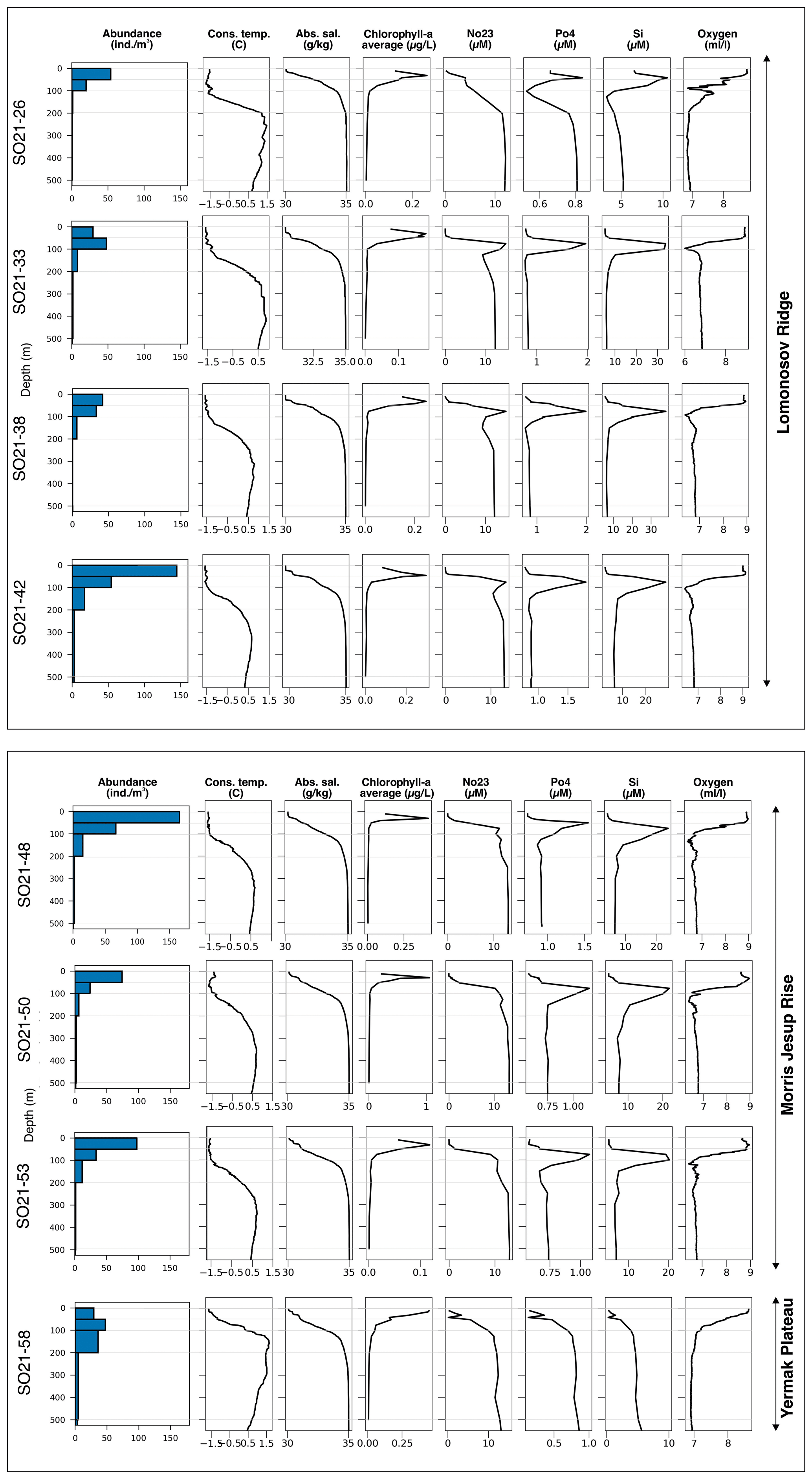
Figure 5 Overview of planktonic foraminifera abundance in relation to environmental parameters at sampling stations during SAS ODEN21. Thin horizontal gray lines indicate the limits of the sampled depth intervals. Blue bars represent abundance of N. pachyderma. At site SO21-58, T. quinqueloba was found at very low abundances below 100 m, and the abundances were lower than the line width of the bars. Chlorophyll-a data are given in Table A1. No23 represents NO₃+NO₂.

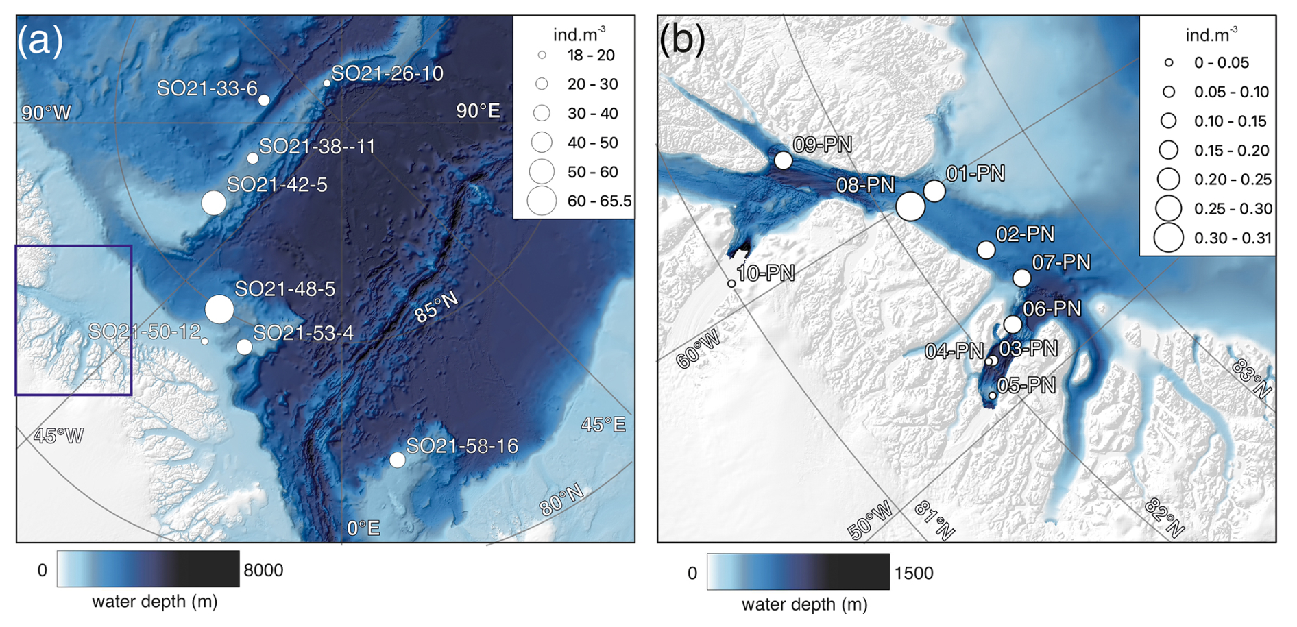
Figure 6 (a) Average abundance of planktonic foraminifera (individuals m⁻³) in the top 200 m for samplings stations obtained during SAS ODEN21. The thin box indicates the general RYDER19 sampling area. (b) Average abundance of foraminifers (individuals m⁻³) in the top 300 m for sites sampled during RYDER19, except for stations 04-PN and 05-PN, where sampling depths reached 408 and 250 m, respectively. No individuals were found at station 05-PN. Note the difference in abundance scale between the two panels.

3.3 Species composition and size distribution

At all stations, except SO21-58-16, the planktonic foraminifera assemblage was monospecific, consisting of N. pachyderma (Plate 1). At station SO21-58-16, a minor proportion of T. quinqueloba was encountered below 50 m, comprising 0.3 %, 3.3 %, and 3.90 % of the assemblage at the 50–100 m, 200–500, and 500–1000 m depth intervals, respectively (Plate 2). Specimens from N. pachyderma species were pristine and showed no signs of dissolution (Plate 1).

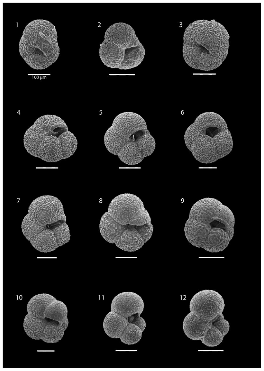
Plate 1 SEM images illustrating the various morphotypes of N. pachyderma: images (1)–(3) show morphotype “Nps-1”; images (4)–(6) show morphotype “Nps-2”; images (7)–(9) show morphotype “Nps-3”; image (10) shows morphotype “Nps-4”; and images (11) and (12) show morphotype “Nps-5”. The specimens shown in images (1), (3), (5), (6), (7), and (8) are from the 200–100 m depth interval at station SO21-58-16. The specimens shown in images (2), (9), and (10) are from the 850–500 m depth interval at station SO21-50-12. The specimen shown in image (4) is from the 200–100 m depth interval at station SO21-50-12. The specimens shown in images (11) and (12) are from the 50–0 m depth interval at station SO21-50-12. All scale bars are 100 µm unless otherwise indicated.

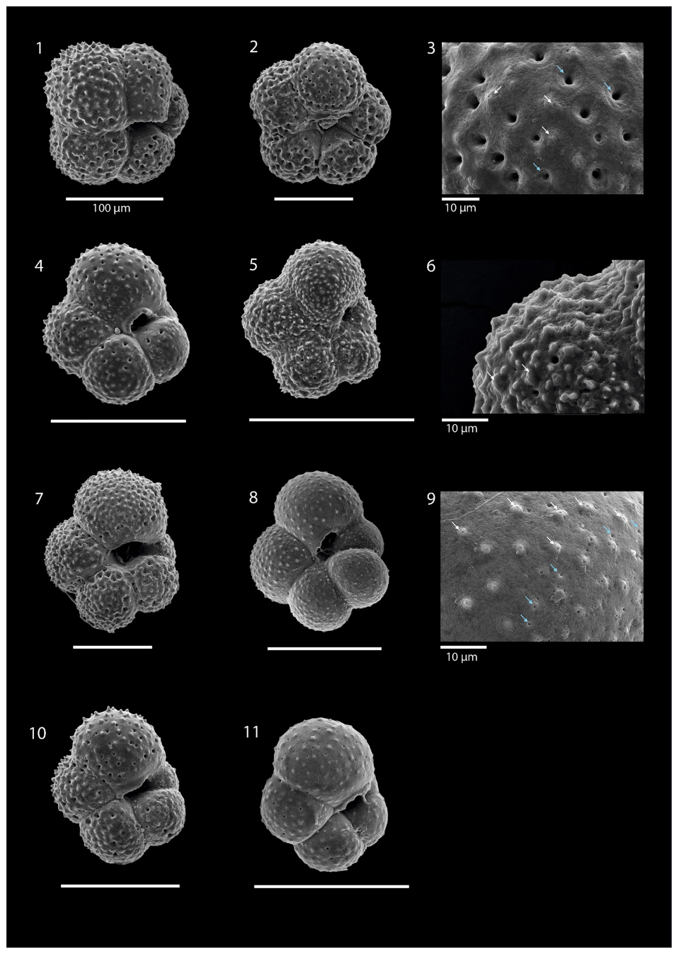
Plate 2 SEM images illustrating Turborotalita quinqueloba: image (1) is sample SO21-58-16 from 500–200 m; images (2) and (4)–(11) are sample SO21-58-16 from 200–100 m; image (3) is the wall texture of image (2); image (6) is the wall texture of image (5); and image (9) is the wall texture of image (8). White arrows indicate spine holes, while blue arrows indicate pores. All scale bars are 100 µm unless otherwise indicated.

All N. pachyderma morphotypes (Nps-1–Nps-5; Eynaud et al., 2009) were observed (Plate 1). In the relatively shallow water depths (the top 100 m), the majority of N. pachyderma individuals were small (range of the mean maximum diameter in the top 50 m = 124–141 µm; average of all means in the top 50 m = 134 µm) and lightly calcified, giving them a translucent appearance under a light microscope, with an appearance similar to Nps-5. At the deeper levels (>200 m), specimens appeared to mostly belong to the more heavily calcified morphotypes Nps-1 to Nps-4 (see Sect. 1 and Plate 1). The range of the mean maximum diameter was 164–261 µm at water depths below 500 m, with an average of all means of 202 µm (Fig. 7).

At station SO21-26-10, cytoplasm-bearing shells were observed at all depths but were predominant in the top 100 m (>75 %; Fig. 8), whereas tests below 200 m were mostly empty; i.e., they were white tests that were settling to the seafloor (<55 %; Fig. 8). Interestingly, the cytoplasm-bearing tests consisted of two types: red and yellow–green (Fig. 8). Some individuals also had both red- and green-colored chambers (Fig. 8). The cytoplasm colors transformed rapidly, and the relatively bright colors faded enough over time (ca. 12 h) to hinder their discrimination. At this site, tests could be rapidly picked, and the color of their cytoplasm was noted immediately (Fig. 8). This revealed that the red-colored individuals were more abundant in the top 50 m (64 % of cytoplasm-bearing tests were red at 0–50 m depth), while the yellow–green type was more abundant at 50–100 m (40 % were red). At 100–200 and 200–500 m, the percentage of tests with red cytoplasm was 60 % and 67 %, respectively, but it should be noted that these numbers are rather uncertain, due to the lower number of tests at these deeper depths (i.e., below 100 m). Due to time constraints, a quantitative assessment of cytoplasm content could not be made at other sites.

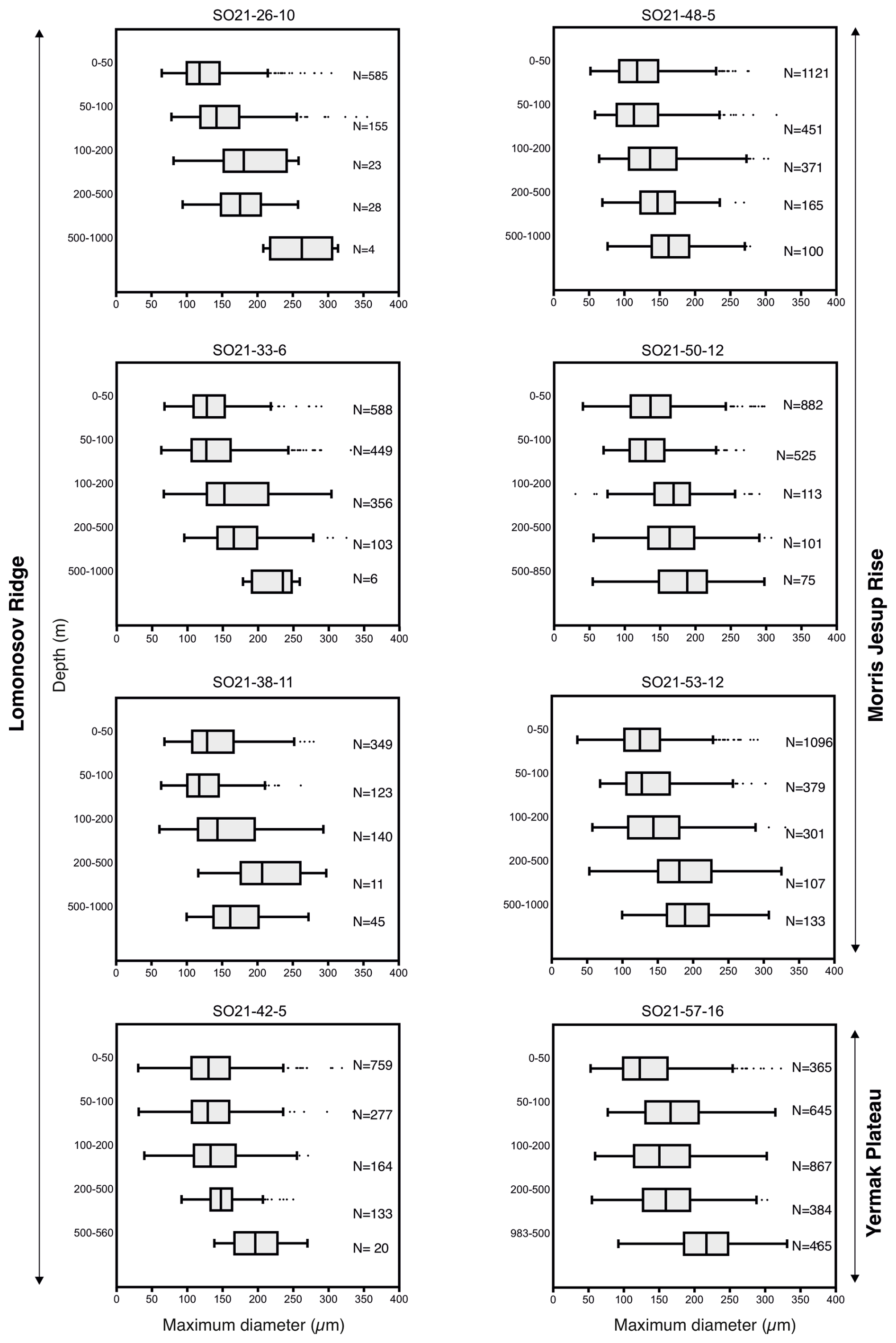
Figure 7 Size distributions of planktonic foraminiferal tests obtained at each station and depth interval (SAS ODEN21). Boxes delineate the interquartile range (IQR: Q1 to Q3); the lines within the boxes represent the median; the upper and lower whiskers delineate Q3 + 1.5 IQR and Q1 − 1.5 IQR, respectively; and dots indicate outliers.

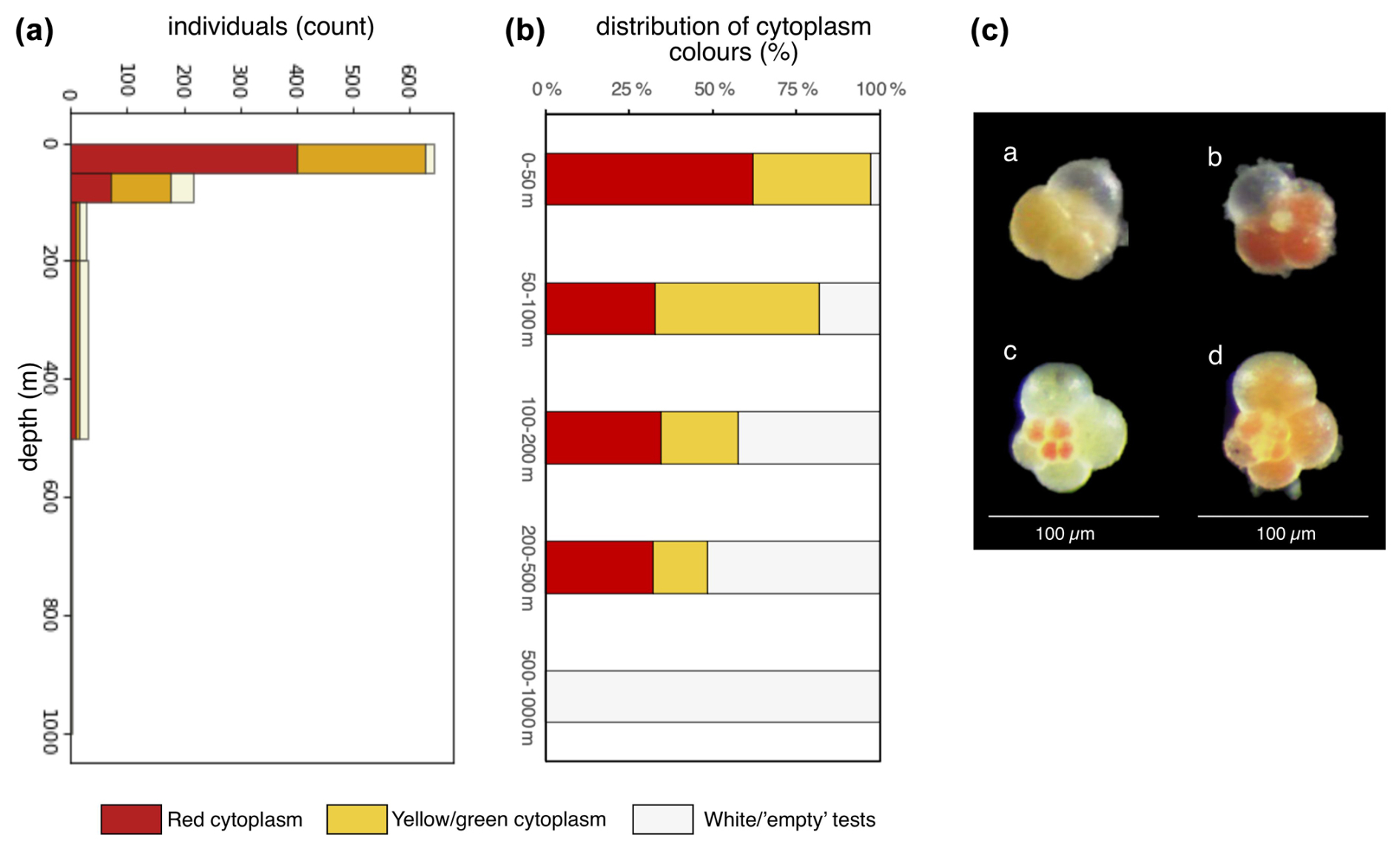
Figure 8 (a) Counts of individuals at station SO21-26-10, shown according to cytoplasm color. (b) Plot of the relative distribution of tests with different cytoplasm content. (c) Example of (a) yellow–green, (b) red, and (c, d) mixed yellow–green- and red-colored cytoplasm in living N. pachyderma. Data are given in Table A2.

4 Discussion

4.1 Current and future composition of planktonic foraminifera in the central Arctic Ocean

Our results show that N. pachyderma is the only species that currently lives and thrives beneath summer sea ice in the region between the North Pole and North Greenland. A few occurrences of T. quinqueloba were found at the northern tip of the Yermak Plateau (SO21-58-16), proximal to the marginal ice zone at depths below 100 m (<4 %). Our results are expected, as N. pachyderma has long been considered the only true polar species that is capable of living in the ice-covered Arctic Ocean (Bé, 1960; Carstens and Wefer, 1992). Turborotalita quinqueloba, on the other hand, is known as a subpolar species that thrives in areas near the sea-ice edge; however, it is not known to reproduce under permanent ice, although it can survive for a limited time under ice-covered conditions (Carstens and Wefer, 1992; Volkmann, 2000; Zamelczyk et al., 2021). In the study of Carstens and Wefer (1992), a significant number of T. quinqueloba individuals were found in the Nansen Basin (up to 55 % south of 83° N and up to 15 % north of 83° N), but these individuals were considered to have been advected along with Atlantic waterbodies, with their reproduction area being further south. More recently, a population of T. quinqueloba was observed underneath the growing winter sea ice of the seasonally ice-free Barents Sea in December (comprising 16 %–67 % of the standing stock, with the rest being N. pachyderma), albeit at very low absolute abundance (<1.5 individuals m⁻³; Zamelczyk et al., 2021).

The Barents Sea is a hotspot for Atlantification (Polyakov et al., 2017), and it was suggested that the T. quinqueloba population under the winter ice in the Barents Sea was probably not reproducing in situ but, rather, had stayed in place after reproduction in open waters and the subsequent onset of winter freezing. From these two studies, it could be anticipated that the rare T. quinqueloba occurrences that we observed near the Yermak Plateau – where Atlantic waters are present at relatively shallow water depths (T>0 °C at 70 m) – can be explained by individuals that survived under the sea ice but were not actively reproducing.

The absence of T. quinqueloba at sites located near the Lomonosov Ridge and North Greenland – located at higher latitude and/or further along the path of Atlantic currents compared to Carstens and Wefer (1992) – demonstrates that T. quinqueloba individuals (or other subpolar species) are not yet present in the central, perennially ice-covered Arctic Ocean and do not survive advection to these sites. Thus, despite the ongoing rapid Arctic warming, retreating sea ice, and intruding Atlantic waters in the Eurasian Basin (Muilwijk et al., 2022), the perennial sea ice that has remained in place currently still only permits one polar species to thrive: N. pachyderma. Net samplings conducted between 1985 and 2015 showed that subpolar species of foraminifera are not yet increasing in the region of the Fram Strait (Greco et al., 2022). In fact, a decrease in subpolar species was found, which the aforementioned work linked to the increased export of Arctic sea ice through this narrow gateway (Greco et al., 2022). It was hypothesized that the invasion of the central Arctic Ocean by subpolar species will commence when ice export comes to a halt and the influence of Atlantic waters in the central Arctic increases (i.e., Atlantification sensu Polyakov et al., 2017). More recent work has showed that subpolar species in general are moving poleward (Chaabane et al., 2024). The data set presented here provides an important baseline for comparison in future studies that will likely document the ongoing transformation. Of particular interest will be tracking the response of N. pachyderma as sea ice disappears.

4.2 Spatial patterns of N. pachyderma abundance

In order to determine the controlling variables, planktonic foraminifera abundances are commonly compared (correlated) with environmental parameters such as sea surface temperature (SST), sea surface salinity (SSS), chlorophyll a, and sea-ice cover (area coverage in percent). In the case of the perennially ice-covered central Arctic Ocean (SAS ODEN21 sites), it should be noted that both SST and SSS in the near-surface waters are strongly dictated by the ice pack, meaning that both SST and SSS were virtually constant across our study sites (ca. −1.7 °C and 30 g kg⁻¹, respectively). Therefore, neither SST nor SSS may explain the variability in standing stock of N. pachyderma across the sites in the central Arctic Ocean. Similarly, the position of the Atlantic Water water mass and its maximum temperature (ca. 0.5 °C) were extremely similar at six out of eight stations (Fig. 4), indicating that they also do not contribute towards the observed variations in abundance across these sites. One consideration to make is that the spatial distribution of planktonic foraminifera populations within a given area is well-known to exhibit “patchiness” – meaning that populations are not distributed uniformly and can be characterized by marked differences in their abundance (e.g., Boltovskoy, 1971). In our survey, we found that the variability in abundance in the central Arctic Ocean ranged between 18 and 65 individuals m⁻³ (average in the top 200 m), indicating a degree of patchiness.

Multivariate statistics can be used to further explore the controlling factors. The results of the final generalized linear model are summarized in Table 2. The analysis revealed significant coefficients (p<0.05) for the predictor variables salinity, temperature, and distance to the sea-ice edge, with the coefficient for chlorophyll being insignificant. The largest coefficient was associated with salinity, suggesting it might represent one of the most the important controlling factors (negative relationship with abundance). However, considering the small range of salinity variability in the 0–50 m depth interval (the interval in which the highest abundances of foraminifera were found) between different sites and the limited size of the data set, the analysis might suffer from overfitting; thus, more data are needed to corroborate these preliminary findings.

Table 2 Summary statistics of the generalized linear model.

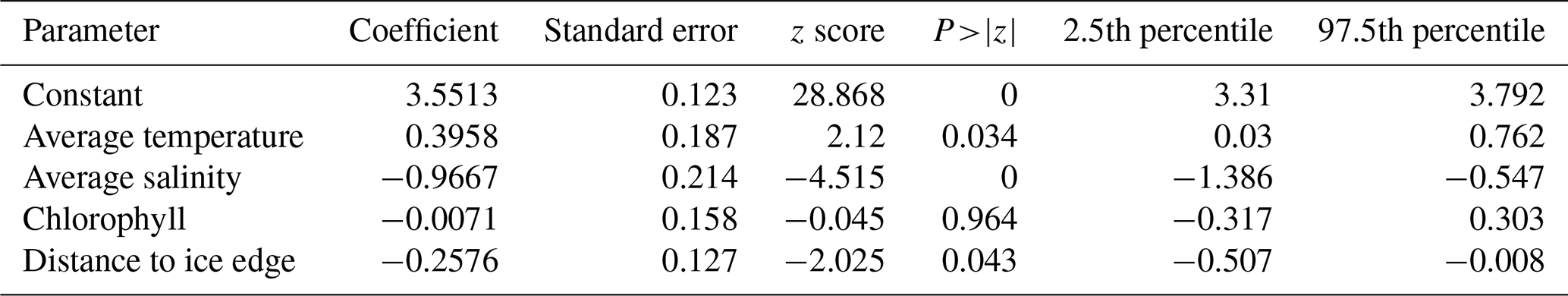
Table 3 Comparison of N. pachyderma abundance (individuals m⁻³) across different sites in the northern North Atlantic.

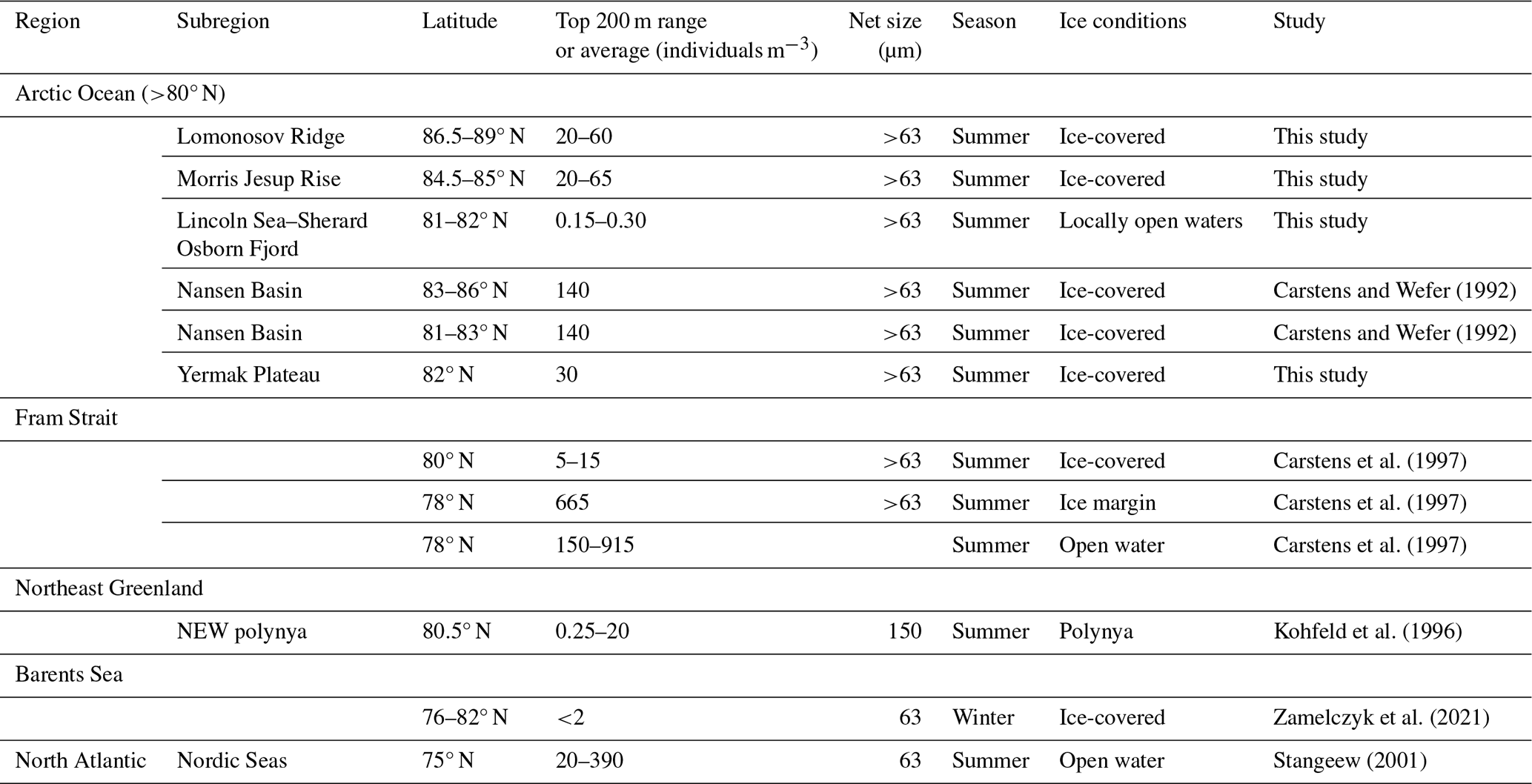
The abundance of N. pachyderma (range 7.8–27.5 individuals m⁻³; averages in the top 500 m) is comparable to that reported at the ice-covered sites between 83 and 86° N reported by Carstens and Wefer in 1992 (range 7.6–15.9 individuals m⁻³; averages in the top 500 m). Based on these two studies alone, it could perhaps be suggested that this range of abundances is typical of N. pachyderma under summer sea ice and that these values have not markedly changed in the past 30 years. However, more studies are evidently needed to characterize both the spatial and temporal (seasonal/annual/decadal) trends of N. pachyderma abundance in the central Arctic Ocean. In order to put these numbers in a broader perspective, we compared our results with the abundance reported near or outside of the seasonal ice edge, (re-)calculating the average in the top 200 m for these studies based on the original data (Table 3). The highest abundances of N. pachyderma have been observed in open waters located near the ice margin, where values were one magnitude higher than under sea ice (150–915 individuals m⁻³; Table 3; Carstens et al., 1997). In the North Atlantic Ocean, the lowest abundances observed along an east–west transect across the 75° N parallel (20 individuals m⁻³) were comparable to those found under sea ice, but maximum abundances were considerably higher (390 individuals m⁻³; Stangeew, 2001). Overall, these observations probably reflect broad-scale spatial changes in primary productivity in the ocean, which is known to reach its highest values in the marginal ice zone (Carstens et al., 1997). Attempting to overcome the difference in mesh size with the study of Bé (1960), we use Berger's “equivalent catch” equation (Berger, 1969), which allows conversions between foraminiferal abundances obtained with different mesh sizes. As the data of Bé (1960) were derived from irregular depth intervals, we selected those samples that differed by <10 m from the depth intervals used in our survey. Data were standardized to a mesh size of 100 µm. For the 0–50 m depth interval, this conversion revealed standardized values ranging between 0.7 and 4.4 individuals m⁻³ (median = 1.58 individuals m⁻³) in Bé (1960), compared to a range of 3.7–20.6 individuals m⁻³ (median = 8.0 individuals m⁻³) in our study. For the 0–100 m depth interval, two data points of 5.4 and 4.3 individuals m⁻³ from Bé (1960) compared to standardized values ranging between 4.6 and 14.5 individuals m⁻³ (median = 5.46 individuals m⁻³) in our study. A plausible explanation for the elevated abundance observed in our study is the difference in sampling timing, as the samples in Bé (1960) were collected in late September and October, likely when population numbers were declining.

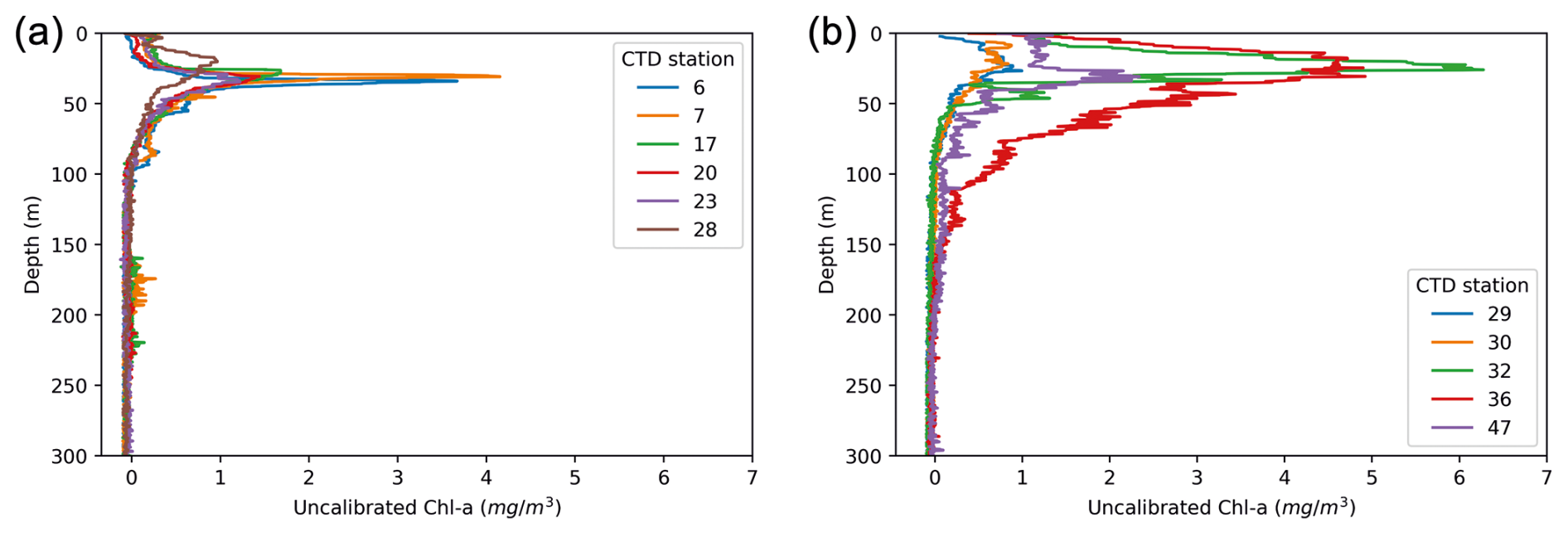
Figure 9 Fluorescence-based estimate of chlorophyll a obtained during the RYDER19 expedition: (a) profiles obtained within Sherard Osborn Fjord; (b) profiles obtained in the Lincoln Sea–Outer Nares Strait. Numbers indicate the names of the CTD stations; see Fig. 3 for their location.

In the region of the Lincoln Sea and adjoining fjords (RYDER19), abundances of planktonic foraminifera were extremely low, comparable to other studies reporting N. pachyderma abundance in shelf environments (Kohfeld et al., 1996; Zamelczyk et al., 2021). Indeed, it is well-known that foraminiferal communities are rare in coastal and shelf environments (Schmuker, 2000), especially at water depths <100 m. Common reasons to explain low abundances in (inner) shelf regions are the high variability in the physical and chemical environment, high turbidity and suspended sediment load, and shallow water depths impeding foraminifer reproduction cycles (Retailleau et al., 2012; Schmuker, 2000; Zamelczyk et al., 2021). Chlorophyll-a concentrations are higher in the Lincoln Sea compared to Ryder Fjord, with the latter exhibiting a narrower and deeper subsurface peak compared to the area outside the fjord (Fig. 9). This is consistent with the somewhat elevated foraminiferal abundances in the Lincoln Sea–Outer Nares Strait region, compared to the very low abundances in Sherard Osborn Fjord (Fig. 6). However, we cannot discern the effect of primary productivity vs. shallow bathymetry here. In the study of Retailleau et al. (2011), it was found that food availability (and freshwater input) were the main factors controlling standing stocks in the shallow Bay of Biscay, rather than depth itself. In contrast, Darling et al. (2007) showed an absence of planktonic foraminifera in the Bering Strait (generally shallower than 50 m), despite high productivity in the region, with similar temperatures and salinities.

4.3 Depth habitat of N. pachyderma

Our results confirm earlier studies, showing the shallow habitat of N. pachyderma underneath perennial sea ice (Bé, 1960; Carstens and Wefer, 1992; Volkmann, 2000). We speculate that the predominance of N. pachyderma in the upper 50–100 m in the central Arctic Ocean is related to food availability (presumably diatoms), which in turn depends on nutrient availability and light penetration limited by the presence of sea ice. Indeed, the chlorophyll-a maximum is typically located between 20 and 40 m, corresponding to the depth interval in which the maximum abundance of tests typically occurs (Fig. 5). A plausible explanation for the relatively high abundances found in the 50–100 m depth interval, located well below the chlorophyll maximum, could be the feeding of N. pachyderma on sinking aggregates, as proposed by the meta-analysis of Greco et al. (2019). The fact that the PSW consists of cold and low-salinity waters does not appear to hinder the resident N. pachyderma populations. These observations confirm previous suggestions that food availability and chlorophyll-a concentration play a key role in determining the depth habitat of N. pachyderma (Greco et al., 2019; Kohfeld et al., 1996; Pados and Spielhagen, 2014; Volkmann, 2000) and that low salinity can be tolerated. This is further supported by the fact that the highest abundances of N. pachyderma in the northern North Atlantic and Arctic Ocean ever reported were found in the highly productive marginal ice zone (Carstens et al., 1997). It is important to note that a distinction should be made between the “main depth habitat” of N. pachyderma and the depth at which the secondary calcite is secreted, which is more important when it comes to interpreting the geochemical signatures of fossil tests in paleoceanography (Tell et al., 2022). At all stations, the test size increased from the surface to 100–200 m depth, and at six out of eight stations, no statistical difference was found between the 100–200 and 200–500 m depth intervals (Fig. 7; Table A3). This pattern would be consistent with reproduction taking place at the base of the productive zone, located at or below 100 m, and would provide some evidence that N. pachyderma does perform ontogenetic vertical migration (Manno and Pavlov, 2014; Tell et al., 2022). On the other hand, large individuals were present at all depths, although rare (Fig. 7), perhaps substantiating that N. pachyderma performs both ontogenetic vertical migration and test growth at fixed depths, in line with the findings of Tell et al. (2022). Nevertheless, this result is to be confirmed and further analyzed with a comprehensive analysis of N. pachyderma morphotypes in a follow-up study. To test whether the populations sampled at the different sites could represent a single reproductive cohort that had undergone synchronous reproduction, we plotted the mean size vs. the date of sampling for the different depth intervals in the top 200 m (Fig. 10). The results showed that there is no significant increase in test size with time and, thus, point towards localized reproduction, rather than a wider reproduction event effecting the whole region (Fig. 10).

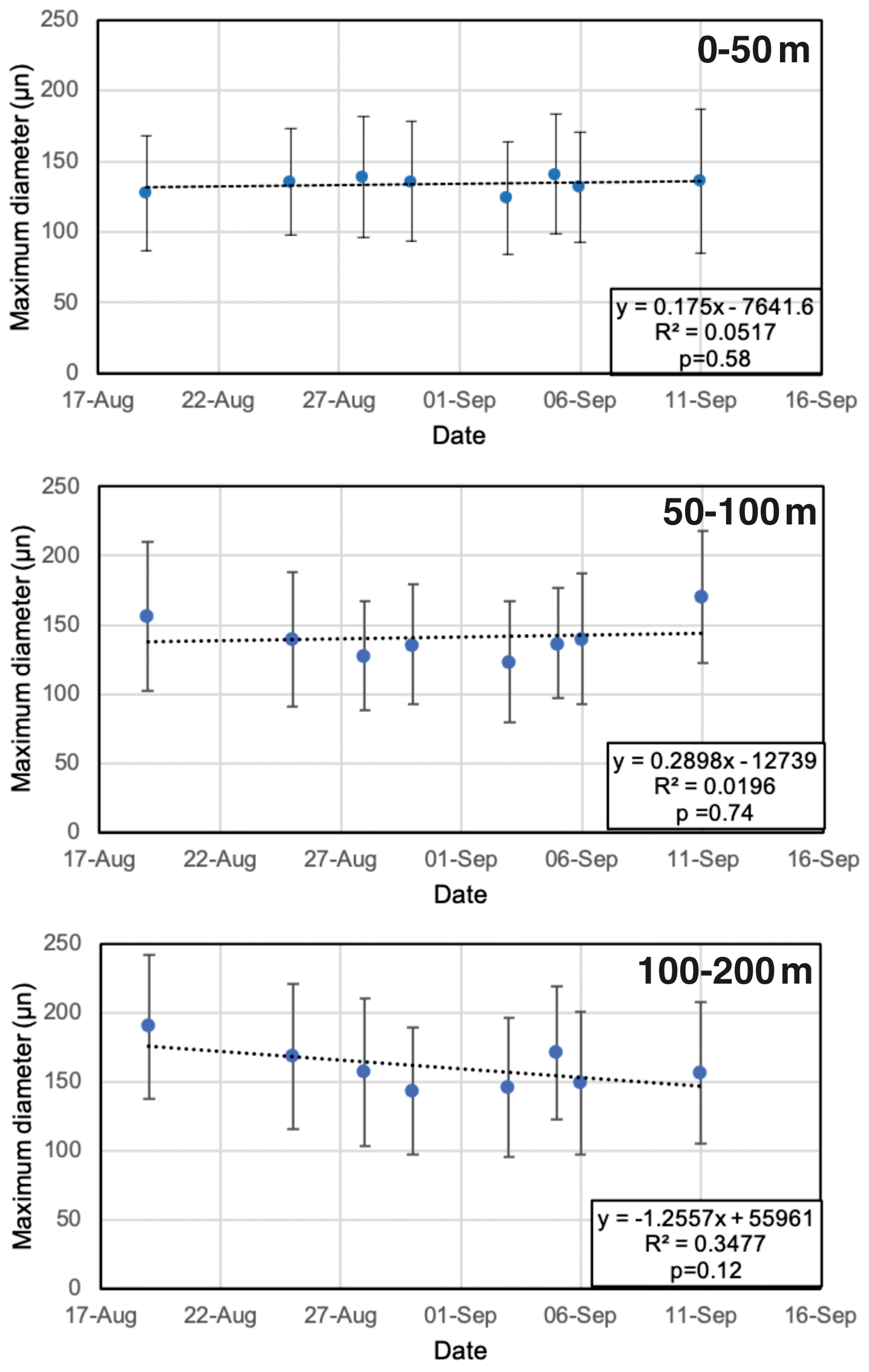
Figure 10 Maximum diameter of test size vs. sampling date during the SAS ODEN21 expedition. Different panels indicate the results for the different depth intervals (0–50, 50–100, and 100–200 m, respectively). Whiskers denote 1 standard deviation. No significant trends were observed.

5 Conclusion

This study details the first systematic survey of live planktonic foraminifera populations in the high Arctic Ocean, at sites near the North Pole, southern Lomonosov Ridge, and the area north of Greenland. While subpolar foraminifera are generally moving poleward (Chaabane et al., 2024), we found that Neogloboquadrina pachyderma was the only species present underneath the perennial ice cover in the region between the North Pole and Greenland at the time of sampling, which would suggest that subpolar species have not yet migrated into the central, perennially ice-covered Arctic Ocean. This is consistent with previous research showing that subpolar species are currently largely “blocked” from entering the central Arctic Basin due to increased sea-ice export through the Fram Strait (Greco et al., 2022), although another potential pathway exists via the Barents Sea. Turborotalita quinqueloba was only observed in very low numbers near the Yermak Plateau and is absent at sites near the Lomonosov Ridge and the Lincoln Sea. This is consistent with its preference for Atlantic waters and abundance at/near the marginal ice zone, which has been widely reported. Overall, this observation emphasizes the prominent oceanographic and climatic changes that must have occurred in the region of the central Arctic Ocean in the past, where evidence of a large-scale T. quinqueloba invasion during at least one previous interglacial is apparent (Vermassen et al., 2023).

Underneath perennial sea ice, N. pachyderma prefers a shallow habitat (in the top 50–100 m), in contrast to the ice marginal zone or areas with open water where it is more abundant at deeper water depths. We suggest that the shallow habitat is due to food availability, i.e., phytoplankton in the photic zone living at shallow depths under the sea ice. The size distribution of N. pachyderma in the water column consistently revealed increasing test sizes with depth. At station SO21-26-10, cytoplasm content was categorized and counted, showing that >75 % of the test were cytoplasm-bearing the upper 100 m, around 50 % were cytoplasm-bearing between 200 and 500 m, and only empty tests were found below 500 m. This could perhaps represent a form of “ontogenetic vertical migration”, with individuals sinking as they grow and reproducing at around 100 m water depth. However, encrusted specimens were observed at all depths (albeit at very low percentages in the top 100 m), and future studies deploying repeated tows would be needed to adequately determine the reproduction pattern of N. pachyderma under the summer sea ice.

As the Arctic Ocean is currently witnessing rapid environmental change, this data set will provide an invaluable baseline for assessing the speed of change in the abundance and composition of planktonic foraminifera communities, in response to sea-ice decline and Atlantification, which are anticipated to intensify in the coming decades. Additionally, the study can serve as a valuable tool for enhancing paleoceanographic investigations that use the sedimentary record.

Appendix A

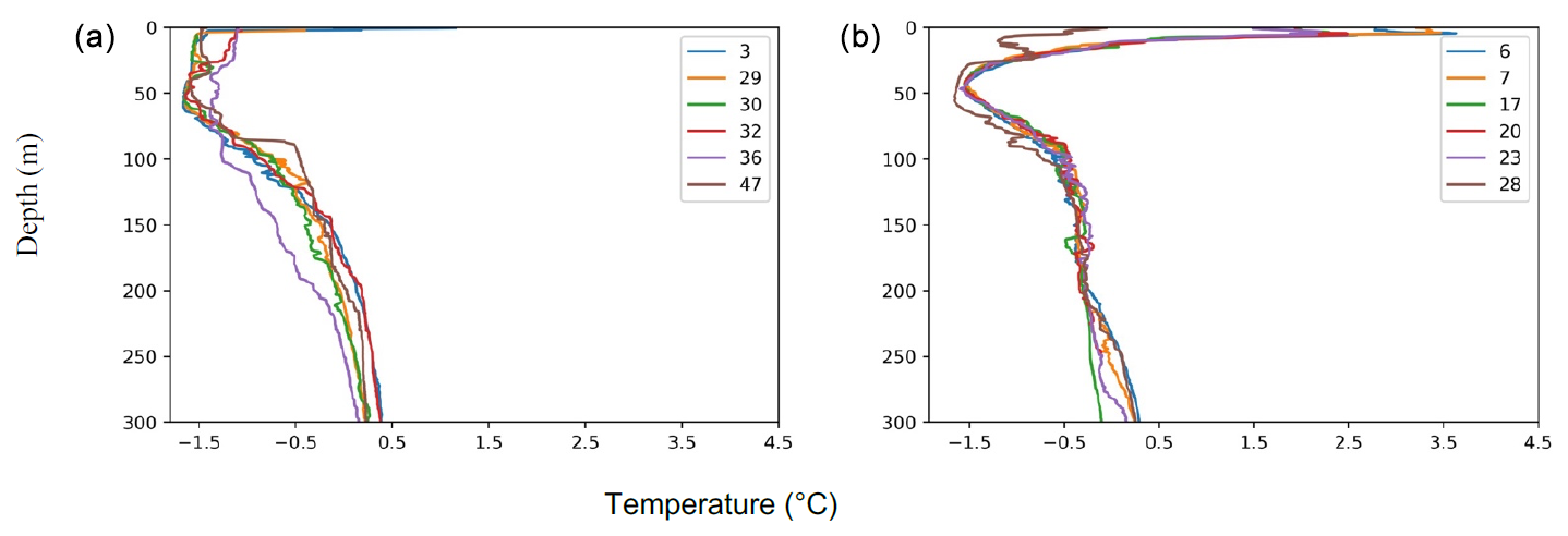
Figure A1 Temperature profiles in the (a) Lincoln Sea–Outer Nares Strait and (b) the Sherard Osborn Fjord. Numbers indicate CTD stations.

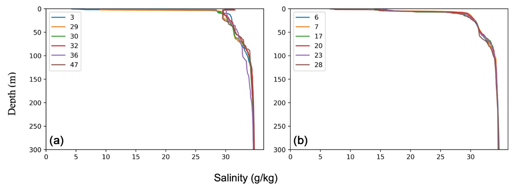
Figure A2 Salinity profiles in the (a) Lincoln Sea–Nares Strait and (b) Sherard Osborn Fjord.

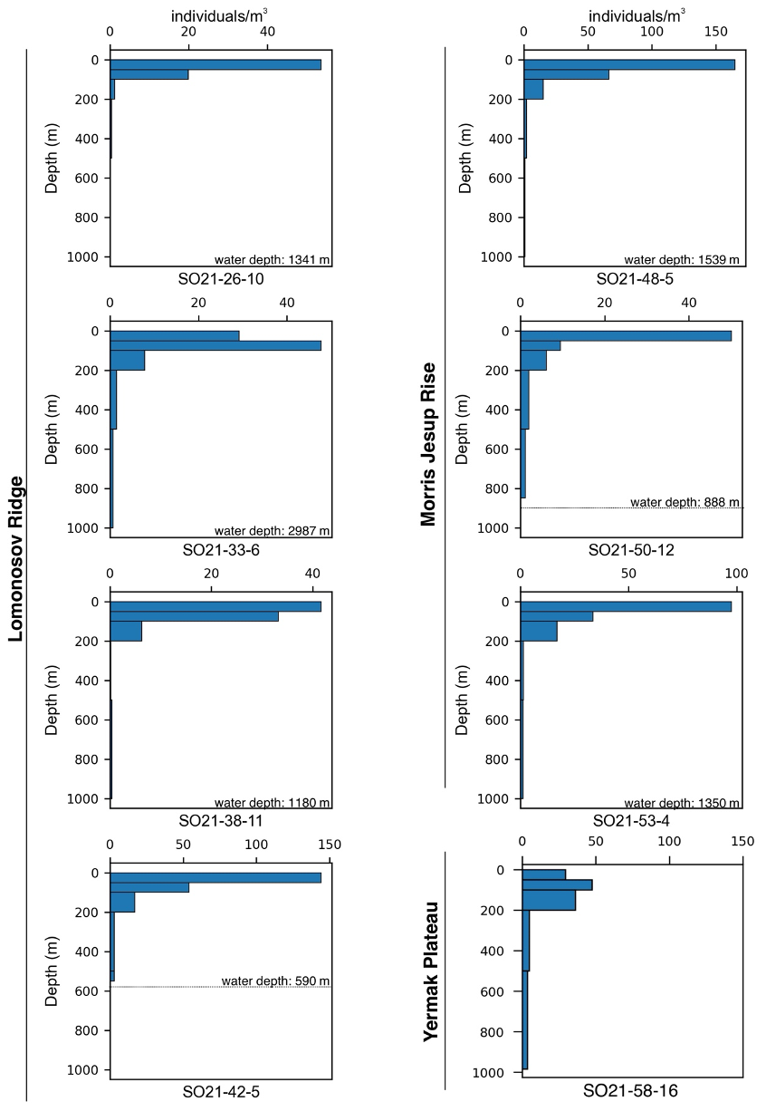
Figure A3 Planktonic foraminifer abundances at each site of SAS ODEN21 (full depth down to 1000 m).

Table A1 Chlorophyll-a (Chl-a) data obtained during the SAS ODEN21 expedition.

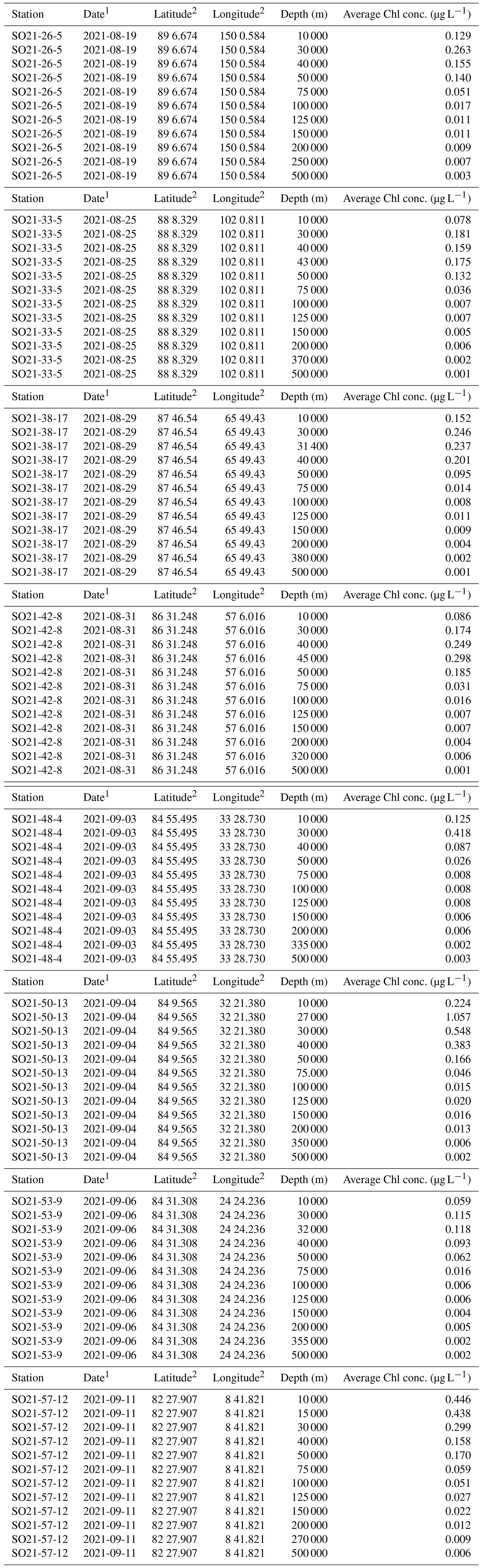
¹ Dates are given in the following format: yyyy-mm-dd. ² Coordinates are given in degrees–decimal minutes (DDM).

Table A2 Data related to test content: red- or yellow-colored cytoplasm or empty tests.

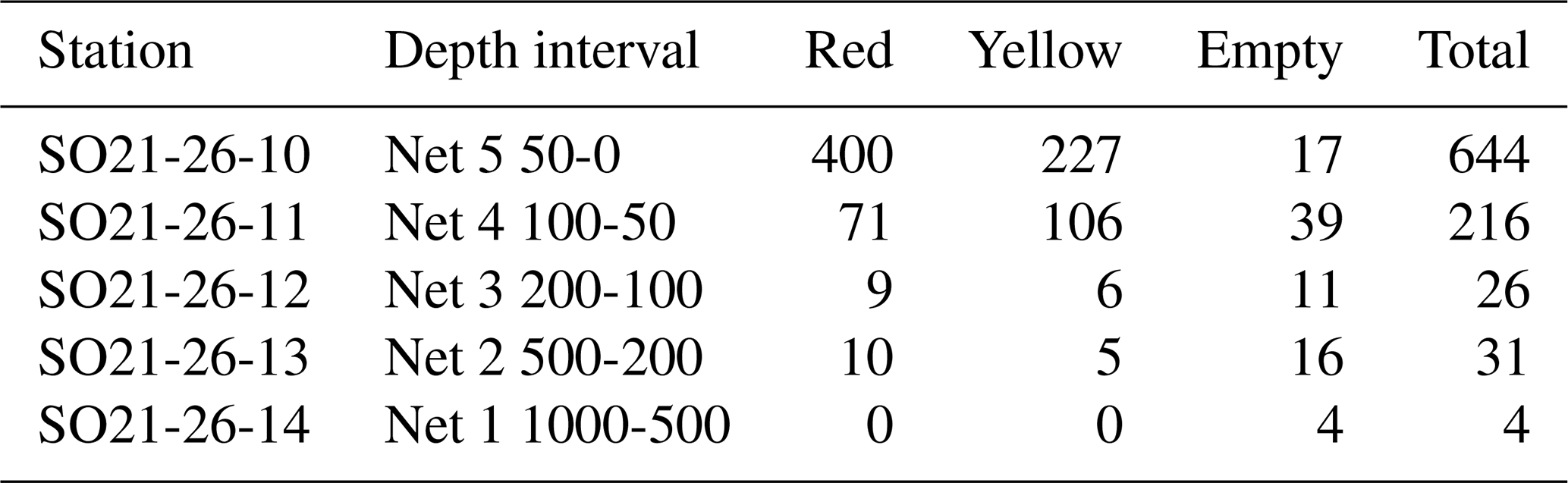
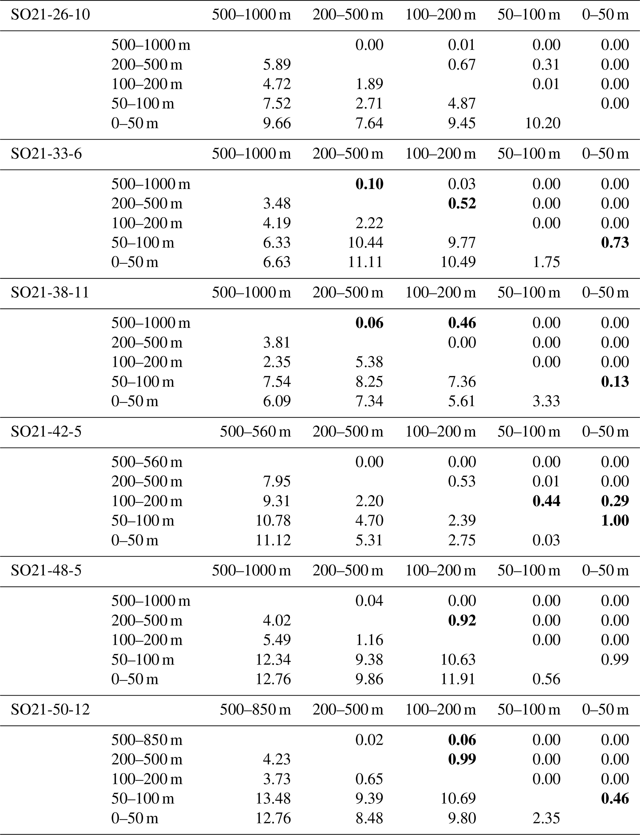
Table A3 Results of Tukey's pairwise comparison, performed on the maximum diameter data, calculated for each station. Numbers above the diagonal indicate p values, numbers below the diagonal indicate Tukey's Q value. Numbers highlighted in bold indicate pairs that are not statistically significant from each other.