the Creative Commons Attribution 4.0 License.
the Creative Commons Attribution 4.0 License.
 | 24 Jun 2025
Impact of stratiform liquid water clouds on vegetation albedo quantified by coupling an atmosphere and a vegetation radiative transfer model
Evelyn Jäkel
André Ehrlich
Michael Schäfer
Hannes Feilhauer
Andreas Huth
Alexandra Weigelt
Manfred Wendisch
This paper investigates the influence of clouds on vegetation albedo. For this purpose, we use coupled atmosphere–vegetation radiative transfer (RT) simulations combining the library for Radiative Transfer (libRadtran) and the vegetation Soil Canopy Observation of Photosynthesis and Energy fluxes (SCOPE2.0) model. Both models are iteratively linked to more realistically simulate cloud–vegetation–radiation interactions above three types of canopy, represented by the spherical, erectophile, and planophile leaf angle distributions. The coupled models are applied to simulate solar, spectral, and broadband irradiances under cloud-free and cloudy conditions, with the focus on the visible to near infrared wavelength range from 0.4 to 2.4 µm. The simulated irradiances are used to investigate the spectral and broadband effect of clouds on the vegetation albedo. Changes in solar zenith angle and cloud optical thickness are found to be equally important for variations in vegetation albedo.
The iterative coupling of both models showed especially that the albedo of canopies with an erectophile leaf angle distribution below optically thin clouds in combination with small solar zenith angles is overestimated when a fixed illumination is assumed. For solar zenith angles less than 50–60°, the vegetation albedo is increased by clouds by up to 0.1. The greatest increase in albedo is observed during the transition from cloud-free to cloudy conditions, with a cloud optical thickness (τ) in the range between 0 and 6. For higher values of τ, the albedo of the vegetation saturates and increases only slightly. The increase in vegetation albedo is a result of three effects that are quantified by the simulations: (i) dependence of the canopy reflectivity on the direct and diffuse fraction of downward irradiance, (ii) the shift in the weighting of downward irradiance due to scattering and absorption by clouds, and (iii) multiple scattering between the top of canopy and the cloud base. The observed change in vegetation albedo due to cloudiness is parameterized by a polynomial function, representing a potential method to include cloud–vegetation–radiation interactions in numerical weather prediction and global climate models.
- Article
(2669 KB) - Full-text XML
- Companion paper
-
Supplement
(427 KB) - BibTeX
- EndNote


The Earth's surface represents an important boundary between the lithosphere and atmosphere, through which energy fluxes (latent and sensible heat, turbulence, gases, aerosol particles, and radiation) are exchanged. Land–surface–atmosphere interactions are a key concern in dynamic modeling (Ardaneh et al., 2025). In the context of radiative processes, the spectral surface albedo α(λ), with λ the wavelength, determines the extent to which solar radiation is absorbed and reflected by the Earth's surface. The surface albedo determines the surplus of energy that is transferred into sensible and latent heat (Moene and Van Dam, 2014). Consequently, the integrated surface albedo α is a central factor in numerical weather prediction models and global climate models. Both types of model simulate the interaction between the atmosphere and the surface, and a realistic representation is crucial since cloud–vegetation interactions via surface flues, for example, can reinforce the thickness of shallow stratocumulus (Freedman et al., 2001; Zhang and Klein, 2013). However, the implementation of vegetation albedo in numerical weather prediction and global climate models is often simplified by using climatologies but neglecting cloud–vegetation–radiation interactions (CVRIs) for example in the Integrated Forecasting System (IFS) of the European Centre for Medium-Range Weather Forecasts (ECMWF) (ECMWF, 2021).
In the visible–near infrared wavelength range (VNIR, 0.3–1.0 µm), bare dry soils typically have a high albedo, while vegetated surfaces usually exhibit a lower albedo, close to zero, particularly for wavelengths shorter than 700 nm. This is a result of the large fraction of photosynthetically active radiation (PAR, e.g., Qin et al., 2018) at wavelengths within the range 0.4 to 0.7 µm (Roderick et al., 2001; Nemani et al., 2003; Dye, 2004; Min, 2005). In contrast, vegetation has a relatively high reflectivity in the shortwave–infrared (SWIR, 1.0–2.5 µm), compared with bare soil that is rich in nutrients and moist (Bowker, 1985). In many cases, natural surfaces are a combination of vegetation on bare soil, for which the albedo at the top of the canopy (TOC) is often considered the most relevant surface for atmosphere–ground interaction.
The TOC albedo is determined by all individual components of the vegetated surface (i.e., leaves, stems, soil, and water content) and the structure, for example, leaf clumping, of the canopy (Jones and Vaughan, 2010). Most important is the leaf area index (LAI, Watson, 1947; Asner, 1998; Jones and Vaughan, 2010), which can range from 0 to 12. It provides a measure of the total one-sided leaf area per unit of ground area, given in units of m2 m−2. The LAI itself depends on the vegetation type, follows an annual cycle, and is modulated by climate conditions (Eugster et al., 2000; Davidson and Wang, 2004, 2005). A lower LAI is typically associated with an albedo that approaches the albedo of the soil, whereas an increase in LAI yields an albedo driven by the properties of the canopy (Jones and Vaughan, 2010). The second most important factor controlling canopy radiation characteristics is the leaf angle distribution (LAD, Baldocchi et al., 2002; Jones and Vaughan, 2010; Verrelst et al., 2015; Yang et al., 2023) in combination with the solar zenith angle. The LAD relates the leaf normal and the direction of the incoming radiation, providing a measure of the sunlit leaf area with respect to the total leaf area. It is therefore a quantitative measure to describe the interaction of incoming radiation with the canopy (Asner, 1998; Stuckens et al., 2009; Vicari et al., 2019). Steeper leaf angles, such as those parameterized by an erectophile LAD, result in lower reflectivity and vice versa (Ollinger, 2011). Therefore, the combination of LAI and LAD determines how the incoming radiation will interact with the canopy and these are therefore important parameters that control CVRIs.
In addition to the surface and vegetation characteristics, the TOC albedo is influenced by the atmosphere, clouds that scatter and absorb radiation, and the solar zenith angle. Optically thin clouds are characterized by high transmission, with radiation preferentially scattered in the forward direction. The remaining fraction is scattered in the backward direction and absorption by water vapor dominates the SWIR part of the solar spectrum. Therefore, incident radiation is attenuated more strongly by absorption in the SWIR part, which causes a shift in the relative weighting of the incoming radiation toward shorter wavelengths (Warren, 1982). Furthermore, scattering at cloud particles leads to an increase in below-cloud diffuse radiation. This is particularly relevant for CVRIs, given that diffuse radiation is reflected in no particular direction (isotropic), whereas direct radiation is partly diffused and partly reflected in a preferred direction (specular or Fresnel reflection).
The impact of clouds on CVRIs with regard to snow and ice surfaces was already investigated in Arctic regions by Wiscombe and Warren (1980), Warren (1982), and Stapf et al. (2020). These authors have demonstrated that an increase of the liquid water path (increase in τ) results in an increase in the broadband surface albedo. Although vegetated surfaces have a lower spectral albedo compared with Arctic regions, it can be expected that clouds have a similar effect on the TOC albedo. For example, Gueymard (2017) showed that clouds can enhance the broadband albedo (this is also called albedo enhancement), by backscattering radiation at the cloud base toward the surface, which leads to an increase in the diffuse downward irradiance. Neglecting potential albedo enhancements in models may cause biases in the simulated radiative budget. Furthermore, it is known that diffuse radiation below optically thin clouds with τ≤6 can penetrate deeper into the canopy and that all parts of the leaves can absorb radiation, not only the leaf areas, and enhance the photosynthesis rate; this is also called the diffuse fertilization effect. A further increase in τ then leads to an overall reduction in downward irradiance and lower photosynthesis rates (Freedman et al., 2001; Min and Wang, 2008; Kanniah et al., 2012). So far, the impact of clouds on TOC albedo and vegetated areas has been neglected in radiative transfer (RT) simulations. Previous investigations focused on the impact of aerosol and molecular scattering, and on reflectance measurements over vegetation (Ranson et al., 1985; Deering and Eck, 1987; Liu et al., 1994). Some studies exist, for example by Lyapustin and Privette (1999), Myhre et al. (2005), and Yang et al. (2020), who used atmospheric RT simulations to calculate surface reflectances depending on different ratios of downward direct and diffuse radiation. However, fixed ratios of direct and diffuse radiation are assumed in reflectance simulations above vegetation (Atzberger, 2004; Kötz et al., 2004; Schaepman-Strub et al., 2006). Consequently, reflectance simulations, which neglect cloud effects, are spectrally distorted compared with, for example, measurements that are performed under cloudy conditions (Schaepman-Strub et al., 2006; Damm et al., 2015). The spectral distortion is a consequence of cloud–radiation interactions including scattering, transmission, or absorption. The relative contribution of these processes depends on the cloud microphysics, cloud morphology, wavelength of the incident radiation, and canopy structure.
Various sophisticated atmospheric radiative transfer (RT) models include clouds in the simulations. This study will utilize the library for Radiative Transfer (libRadtran, Emde et al., 2016). While atmospheric RT models, for example the Moderate Resolution Atmospheric Transmission model (MODTRAN, Berk et al., 2014), have been coupled with vegetation RT models, like the Soil Canopy Observation of Photosynthesis and Energy fluxes version 2 (SCOPE2.0, Yang et al., 2020), none of the previous approaches considered clouds in these simulations. Some studies have either investigated the radiative effects of clouds over different land types and changing forests (Betts, 2000; Bounoua et al., 2002; Cerasoli et al., 2021), while other studies have concentrated on the RT within or at the TOC, taking into account the properties of the canopy itself (Sinoquet et al., 2001; Majasalmi and Rautiainen, 2020; Henniger et al., 2023).
As a result of this discussion and since the radiation interactions of clouds and vegetation have not been explicitly simulated yet, the following four questions are addressed in this paper:
- i.
How strongly do clouds impact the spectral and broadband albedo of vegetation?
- ii.
How large are the improvements in broadband albedo achieved by coupling atmospheric and vegetation RT models?
- iii.
Can we separate and quantify individual coupling effects?
- iv.
What are the consequences for cloud radiative effects?
To answer the above questions and to systematically investigate CVRIs, we iteratively coupled the atmospheric RT model libRadtran and the vegetation RT model SCOPE2.0 to investigate the radiative interaction of clouds and vegetation. The model coupling provides a more realistic input to the atmospheric radiative transfer model libRadtran by incorporating the vegetation albedo from SCOPE2.0, while the simulated spectral downward irradiance from libRadtran fed into SCOPE2.0 accounts for scattering and absorption by clouds.
The model coupling is introduced in Sect. 2 by first defining the fundamental properties to describe the RT in the atmosphere and vegetation, and its interaction with the surface. Then the general model set-up is outlined and the basics of the RT models libRadtran and SCOPE2.0 are introduced. The coupling itself is realized by an iterative approach that is applied for different test cases. Section 3 presents the simulations, with Sect. 3.1 outlining the differences between uncoupled and coupled simulations. In Sect. 3.2 the spectral effects of clouds on the vegetation albedo are shown and in Sect. 3.3 the impact of clouds on the forest albedo is quantified by running the coupled model for a set of scenarios, including a range of clouds, solar zenith angles, and leaf area indexes, and three different leaf angle distributions. In Sect. 3.4 the contributions of multiple-scattering and directional effects to the change in the vegetation albedo are separated. A discussion about the implications of a fixed vegetation albedo for the top-of-canopy radiative budget is given in Sect. 3.5 and Sect. 3.6 outlines the limitations of the idealized simulations. The results are summarized in Sect. 4.
2.1 Terminology
We provide the basic radiometric definitions, terminology, and abbreviations, which mainly follow Wendisch and Yang (2012), Schaepman-Strub et al. (2006), and Jones and Vaughan (2010), to facilitate the understanding of this paper.
Radiant energy passing through an area element within a certain time interval that originates from a certain solid angle element is defined as the spectral radiance I(λ) in units of W m−2 nm−1 sr−1. The spectral irradiance F(λ) is defined by the radiant energy passing through an area element within a certain time interval. F(λ) is given in units of W m−2 nm−1 and can be separated into the upward F↑(λ) and downward F↓(λ) components. Both are defined with respect to a horizontal surface area from either the lower or upper hemisphere, respectively. F↓(λ) is composed of the direct solar irradiance , transmitted through the atmosphere without any interaction, and the diffuse irradiance , scattered at least once by atmospheric constituents, and thus:
The direct fraction in relation to F↓(λ) is quantified by the ratio fdir(λ) defined by
In theory, the ratio fdir(λ) ranges between a value of 0, indicating no direct radiation, and a value of 1, indicating pure direct radiation. However, pure direct radiation is unrealistic under normal atmospheric conditions. The broadband direct fraction fdir is obtained by
Calculating the ratio between F↑(λ) and F↓(λ) yields the spectral albedo α(λ) (unitless):
The spectrally integrated albedo α (unitless) is obtained by weighting the spectral albedo with F↓(λ) and integrating over the wavelength range from λ1 to λ2, as
To obtain the broadband solar albedo, α(λ) is integrated from λ1=0.2 to λ2=4.5 µm, which is equivalent to measurements with broadband albedometers, i.e., a set of upward and downward looking pyranometers. In the following, the integration of α(λ) is limited to the wavelength range from 0.4 to 2.4 µm because of model constraints and indicated as αBB. Often, natural surfaces, such as forests, are a combination of vegetation on bare ground, for which the albedo at the TOC is often considered to be the most relevant surface for atmosphere–ground interaction. In this case, the albedo at the TOC is simply referred to as the albedo α(λ).
The primary parameter that describes the radiative properties of a canopy is the leaf area index (LAI, Watson, 1947; Asner, 1998; Jones and Vaughan, 2010). It is a measure of the total one-sided area of leaves per unit ground area, given in units of m2 m−2, and can range between values from 0 to 12. The LAI depends on vegetation type and is subject to annual and seasonal variations as well as weather and climate conditions (Eugster et al., 2000; Davidson and Wang, 2004, 2005).
The second most important parameter that controls the RT in the canopy is the leaf angle distribution (LAD, Baldocchi et al., 2002; Jones and Vaughan, 2010; Verrelst et al., 2015; Yang et al., 2023). The leaf angle of an individual leaf is defined as the angle between the leaf normal and the zenith. The LAD is obtained over all individual leaf angles of a leaf ensemble. The LAD ultimately determines the sunlit area of a leaf with respect to the one-sided total leaf area and, thus, the area where reflection and absorption occurs (Asner, 1998; Stuckens et al., 2009; Vicari et al., 2019). Goel (1988) proposed six LADs, with three common types: the spherical distribution, where all leave orientations have the same probability; the erectophile distribution, where the majority of leaves have a preferred vertical alignment; and the planophile distribution, where most of the leaves are horizontally aligned. The erectophile and planophile LAD represent two extreme cases among the LADs. Within models, LADs are described by two-parameter beta distributions, trigonometric functions, or ellipsoidal distributions (Goel and Strebel, 1984; Jones and Vaughan, 2010).
The extinction of radiation by scattering and absorption in homogeneous media can be approximated by the turbid medium model (Kubelka, 1931; Kokhanovsky, 2009; Jones and Vaughan, 2010). Within the Earth's atmosphere, scattering and absorption by clouds, aerosol particles, and gas molecules is quantified by the optical thickness τ(λ), which depends on the volumetric extinction coefficient βext(λ) (given in units of m−1). Subsequently, the cloud-induced optical thickness is simply referred to as τ(λ). In the simplified case of a homogeneous atmosphere, the extinction of direct solar radiation follows the Beer–Bouguer–Lambert law, which can be expressed as
with the path length z. The extinction of I(λ) at z is then expressed by
where I(λ)0 is the direct radiance at the top of the atmosphere (TOA); I(λ)z is the direct radiance at a certain penetration depth with z=0 at TOA. Monsi (1953) proposed a similar concept to treat the RT in homogeneous vegetation. The attenuation of direct radiance at penetration depth z is then caused by leaves, which are considered as point scatterers (Kubelka, 1931; Jones and Vaughan, 2010). Then, the extinction coefficient βext(λ) in Eqs. (6) and (7) is replaced by kext, here called the vegetation extinction coefficient. The penetration depth z is replaced by the LAI. A brief overview of kext estimates and the attenuation of I(λ) within vegetation is provided in Appendix D.
2.2 Iterative coupling
The albedo of a surface is primarily controlled by the structural parameters of the vegetation, but is also driven by atmospheric factors, namely the direct and diffuse components of the incident radiation F↓(λ), and the angle of the incident radiation on the surface. Please note that the incident angle, in the following referred to as θ, is not necessarily equal to the solar zenith angle θ0. Both angles are approximately equal for cloud-free atmospheres and low aerosol particle concentrations but increasingly deviate for overcast conditions (e.g., see Wiscombe and Warren (1980)). Atmospheric RT models frequently use standard libraries of forest albedo, such as the library of the International Geosphere Biosphere Programme (IGBP; Loveland and Belward, 1997). Conversely, vegetation RT models do simulate the RT in and directly above the canopy but neglect scattering and absorption by clouds in the atmosphere, and assume a fixed ratio of direct to diffuse ratio of F↓(λ). By iteratively coupling vegetation and atmospheric RT models, the atmospheric RT model provides more realistic solar spectra of and , while the vegetation RT model provides a more realistic albedo above canopies that is used as the input for the atmosphere RT model in the next iteration. In the proposed set-up, the iterative coupling is achieved through the exchange of and , and α(λ), between the two models. More specifically, and from the atmosphere RT model provide the input to the vegetation RT model. The simulated F↑(λ), with and from the atmosphere RT model, allows the calculation of an updated α(λ), used as the input for the next simulation with the atmosphere RT model.
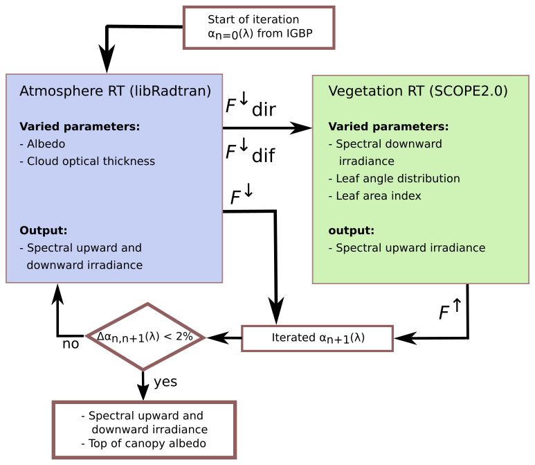
Figure 1Schematic of coupled atmosphere (blue) and vegetation (green) radiative transfer models. The RT models are coupled via the exchange of spectral, direct , and diffuse downward irradiance, and the top-of-canopy albedo α(λ). The atmospheric RT model is started with a first guess albedo from the IGBP database. When the convergence criterion is met, the iteration is stopped.
Figure 1 shows a schematic of the proposed iterative coupling. Each simulation run is realized by n iterations, where each iteration includes a calculation from the atmospheric RT (blue box) and the vegetation RT (green box). The first iteration starts with the atmospheric RT model, using a first guess, the spectral surface albedo of forests, here the “mixed-forest” spectral surface albedo from the IGBP database, to obtain the simulated upward and downward Fn(λ) of the first simulation (n=0). The direct and diffuse components of are then input in the vegetation RT model, which is therefore initialized with representing the atmospheric conditions including clouds, instead of a default F↓(λ) and direct–diffuse ratio. The new from the vegetation RT model is then used to calculate αn+1(λ) at the TOC using Eq. (4). The updated surface albedo provides the input for the atmospheric RT model in the next iteration step. We call an iteration successfully converged if the relative difference between iteration n and n+1 for 90 % of the wavelengths is less than 2 % for the albedo. Formalized, this can be expressed as
with P90th the 90th percentile, αn(λ) the spectral albedo of the previous iteration step, and αn+1(λ) the spectral albedo of the current iteration. In this study two iterations were found to be sufficient for all canopy and cloud parameter combinations. This is consistent with Wendisch et al. (2004), who also used an iterative approach to determine the surface albedo from airborne observations. They found that after two iterations, even for rough first estimates of α(λ), the retrieved albedo is close to the true surface albedo. In most applications the surface albedo is approximately known, providing a reasonable initial guess, and reducing the number of required iterations.
2.2.1 Atmospheric radiative transfer model libRadtran
The atmospheric RT model library for Radiative Transfer (libRadtran, Emde et al., 2016) is applied to simulate the RT through the atmosphere above the canopy. The one-dimensional solver “Discrete-Ordinate-Method Radiative Transfer” (DISORT, Stamnes et al., 1988; Buras et al., 2011) is selected to calculate the RT using 12 streams, which are supposed to be sufficient to study irradiances. Since one-dimensional RT models assume homogeneous clouds that best resemble stratiform clouds, this study focuses on low- and mid-level warm stratus and altostratus, which cover between 4 % and 12 % of the entire globe at any time (Eastman et al., 2011). These clouds are represented by liquid water clouds with a fixed cloud base at an altitude of 3 km and a cloud top altitude of 3.5 km, representative of mid-latitude continental clouds. The effective cloud droplet radius is fixed to 10 µm, as typically found in such clouds over continents (Stephens, 1994; Frisch et al., 2002; Aebi et al., 2020). The liquid water path is modified such that a desired value of τ at 550 nm, τ(λ=550 nm), is achieved and all other values are scaled accordingly, considering the wavelength dependence of τ. The cloud optical thickness τ is varied between values of 0 and 80 to simulate natural conditions of stratus clouds ranging from cloud-free to densely overcast, and to include values of τ at which the cloud top reflectivity saturates (King, 1987; Nakajima et al., 1991; Tselioudis et al., 1992). Subsequently, τ(λ=550 nm) is referred to as τ for simplicity. Spectral calculations of F↑(λ) and F↓(λ) are performed for a wavelength range from 0.4 to 2.4 µm. This range was previously used as the integration limits for fdir and α in Eqs. (3) and (5). The incoming spectral irradiance at TOA is represented by the solar reference spectrum provided by Coddington et al. (2021). The solar zenith angle θ0 is varied between 25 and 70° to cover the typical range of the mid-latitudes. Molecular absorption is considered by using the “medium” resolution parameterization from Gasteiger et al. (2014). A default aerosol distribution after Shettle (1989) is applied, which represents aerosol of rural type in the boundary layer, background aerosol above 2 km during spring–summer, and a visibility of 50 km. Atmospheric profiles of air temperature, humidity, and gas concentration are represented by the mid-latitude summer profile “afglms” after Anderson et al. (1986). Absorption by water vapor and other atmospheric trace gases are included in the simulations (Anderson et al., 1986; Emde et al., 2016). The initial run of libRadtran is initialized with the “mixed-forest” albedo α taken from the IGBP database (Loveland and Belward, 1997), which is then replaced by α(λ) from SCOPE2.0. An output altitude of 40 m above ground is selected to characterize the downward radiation (direct and diffuse) just above the canopy. A typical input file that is used to initialize the libRadtran simulations is provided in the Supplement.
2.2.2 Vegetation radiative transfer model SCOPE2.0
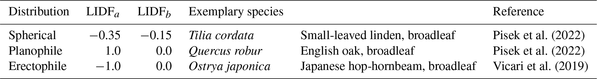
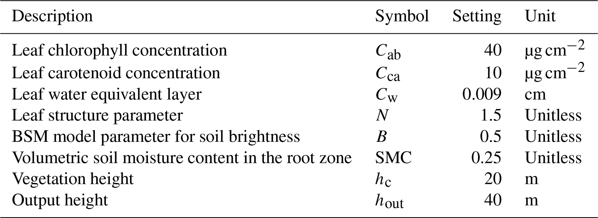
The solar RT through vegetation is simulated with the Soil Canopy Observation of Photosynthesis and Energy fluxes (SCOPE2.0 Yang et al., 2021). SCOPE2.0 is an updated version of SCOPE, which has been developed for forward modeling radiances and albedo for satellite vegetation retrievals. SCOPE2.0 treats the RT by combining the leaf RT model Properties Spectra (PROSPECT) with the canopy RT model Scattering by Arbitrarily Inclined Leaves (SAIL Verhoef, 1984; Yang et al., 2017, 2021). At their core, these models are based on the turbid medium approach (Yan et al., 2021). In SCOPE2.0 the soil albedo assumes different soil types, where the moisture dependence is determined by the Brightness–Shape–Moisture (BSM) model (Verhoef et al., 2018; Yang et al., 2020). The default BSM model parameter for soil brightness B= 0.5 is used. The optical properties of individual leaves are provided by the Fluorescence Spectra (Fluspect) model, which developed out of PROSPECT (Vilfan et al., 2016, 2018). Simulation of vegetation chlorophyll fluorescence was activated in the simulations. The upward directed F↑(λ) and the canopy albedo at the TOC is simulated as a superposition of the soil and the contribution from the vegetation. Simulations in the solar part of the spectrum with SCOPE2.0 are generally limited to the wavelength range from 0.4 to 2.4 µm. Consequently, the calculation of spectral α(λ) and broadband albedo αBB are restricted to the same wavelength range, where αBB is calculated from Eq. (5). The optical properties of vegetation primarily depend on the vegetation type, tree species, tree age, canopy structure, and solar zenith angle (Liang et al., 2005; Stenberg et al., 2013; Hovi et al., 2017; Zheng et al., 2019). To consider different vegetation states during the annual cycle, the LAI is varied between 1 and 5 m2 m−2, with LAI = 3 m2 m−2 as the default. The lower boundary is selected to include sparse canopies and the upper boundary is selected to include the largest sensitivity of F↑(λ) and αBB on LAI. For LAI > 5, F↑(λ) and αBB are expected to become insensitive to changes in LAI, since reflectances start to saturate (Houborg and Boegh, 2008). In SCOPE2.0 the LAD is represented by a linear combination of trigonometric functions in the leaf inclination distribution function (LIDF) (Verhoef, 1998), which is specified by the two parameters LIDFa and LIDFb. Three different LADs – spherical, planophile, and erectophile – are simulated, with parameters LIDFa and LIDFb provided in Table 1. Table 2 summarizes the relevant parameters for vegetation RT simulations in the visible–near infrared wavelength range that are kept constant in the simulations.
Pisek et al. (2022)Pisek et al. (2022)Vicari et al. (2019)Table 1Leaf angle distribution (LAD) and corresponding values for the leaf inclination distribution function parameters LIDFa and LIDFb that were used to parameterize the orientation of the leaves (Yang et al., 2021).
3.1 Differences between uncoupled and coupled simulations
Analyzing the coupled simulations, it is found that the sensitivity of the simulated spectral and broadband F(λ) and α(λ) is greatest below τ=6, thus, defining the range of τ that is most interesting for understanding CVRIs. Appendix A provides a brief discussion of the response of αBB for τ>6.
The necessity to initialize vegetation RT simulations with realistic F↓(λ) and the need for RT model coupling are demonstrated in Fig. 2a and b, which show an example of and α(λ) at different stages of model coupling and iteration. The simulations are performed for an intermediate θ0=45° and τ=2, where diffuse radiation dominates but direct radiation is still contributing to the radiation field. Under cloud-free conditions (black line), downward diffuse irradiance above the canopy is generally small, except at wavelengths below 700 nm, where the contribution from Rayleigh scattering increases. Including clouds in the atmospheric RT model increases (red line) compared with the cloud-free case due to scattering at cloud particles. The spectrum is characterized by water-vapor absorption in the wavelength bands 933–946, 1118–1144, 1350–1480, and 1810–1959 nm. Coupling of libRadtran and SCOPE2.0 iteratively results in (orange line), which is slightly higher compared with the uncoupled simulations, since multiple scattering enhances . Relative differences, given in the subpanel of Fig. 2a, of up to −5 % are identified between the uncoupled and coupled cloudy simulations for wavelengths between 700 and 1200 nm, where the total F↓ and α(λ) are generally largest.
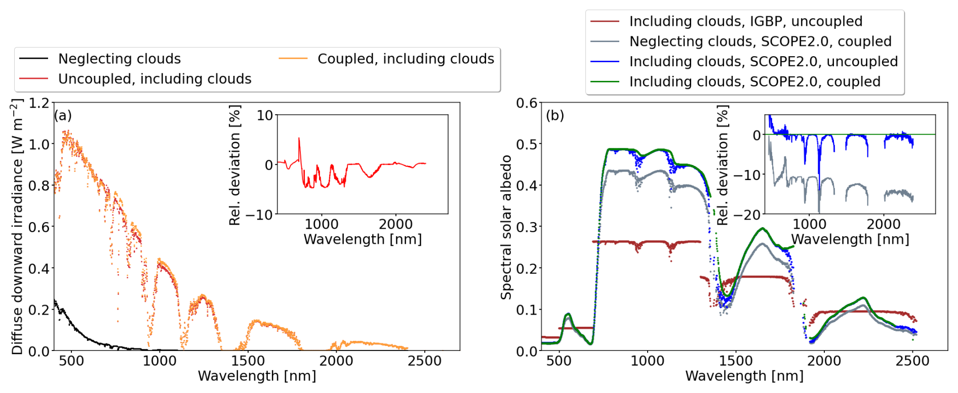
Figure 2(a) Spectral downward diffuse irradiance simulated for cloud-free conditions (τ=0) and no model coupling (black). simulated for a value of τ=2 but still in the uncoupled set-up (red). simulated for a value of τ=2 and with the coupled set-up (orange). (b) Spectral albedo α(λ) simulated using the “mixed-forest” albedo from the IGBP database for τ=2 and uncoupled simulations (brown). α(λ) from coupled simulations but neglecting clouds (gray). α(λ) from uncoupled simulations including clouds with τ=2 (blue). α(λ) from coupled simulations including clouds with τ=2 (green). Subplot in (a): the relative difference between “uncoupled, including clouds” and “coupled, including clouds” with respect to the coupled simulations. Subplot in (b): the relative difference between “neglecting clouds, SCOPE2.0, coupled” and “including clouds, SCOPE2.0, uncoupled” with respect to “including clouds, SCOPE2.0, coupled”.
Since clouds modify F↓(λ) spectrally and fdir(λ), they also impact α(λ). Figure 2b shows α(λ) during different model set-ups and iterations. A generic α(λ) is provided by the IGBP database (brown line), which was also used as a first guess to initialize the libRadtran simulations. The radiation is reflected isotropically and does not take into account any dependence on the incident angle or the presence of clouds. Running SCOPE2.0 freely without any constraints from the atmosphere, i.e., assuming a cloud-free atmosphere, a better resolved α(λ) is obtained (gray line). By providing spectra of direct and diffuse F↓(λ) that represent cloudy conditions with τ=2, a higher α(λ) is obtained (blue line), which is caused by the greater fraction of diffuse radiation. Relative differences of about −2 % to 15 % are determined. Simulations at this stage of the iteration still neglect CVRIs. Coupling both models under cloud conditions results in α(λ) (green line), which is slightly further enhanced, compared with the blue line, due to multi-scattering between TOC and cloud base. For the given example, the relative differences range between 3 % and −5 %, with respect to the fully coupled simulations (see subpanel Fig. 2b). The following analysis will systematically examine the discrepancies in spectral and broadband F(λ) and α between uncoupled and coupled simulations, depending on θ0 and the optical properties of clouds and vegetation.
3.2 Sensitivity of spectral surface albedo
Radiation that interacts with clouds is scattered and absorbed. Wavelengths below 900 nm that are outside the absorption bands are primarily affected by scattering from molecules, aerosol, and cloud particles (Mie, 1908), while absorption dominates longer wavelengths. Example simulations of direct and diffuse F↓(λ) for four different values of τ are given in Appendix B. Here we express the wavelength-dependent effects of scattering and absorption on the total F↓(λ) by the illumination ratio , where represents cloudy (index “c”) simulations, while represents cloud-free (index “cf”) simulations. It is important to note that simulated , with τ=0, simultaneously represents simulations that neglect the presence of clouds in the atmospheric RT.
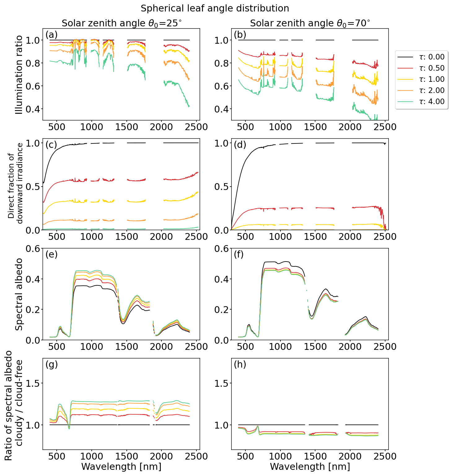
Figure 3Simulations for solar zenith angles of θ0=25° (left column) and θ0=70° (right column), a spherical leaf angle distribution, and a leaf area index LAI=3. Cloud optical thickness τ is indicated by the colored lines. From top to bottom: (a, b) illumination ratio (unitless) of spectral downward irradiance F↓(λ) under cloudy conditions (index c) in relation to cloud-free conditions (index cf); (c, d) direct fraction fdir(λ) of total downward irradiance F↓(λ); (e, f) spectral albedo α(λ) (unitless); (g, h) illumination ratio (unitless) of spectral α under cloudy conditions (index c) in relation to cloud-free conditions (index cf).
Figure 3a and b show the illumination ratio for the extreme cases of θ0=25 and 70°, respectively. The presence of clouds results in an illumination ratio that is less than 1, since radiation is scattered at the cloud top and absorbed inside the cloud. For the same cloud, a value of θ0=70° results in a smaller ratio compared with θ0=25°, due to the longer path length through the cloud, which increases extinction. The longer path length for θ0=70° also increases the sensitivity of the illumination ratio to τ. The extinction of radiation by absorption at longer wavelengths exceeds the extinction by scattering at shorter wavelengths. In relative terms, the decrease in the radiation above the cloud compared with the radiation below the cloud is more pronounced at longer wavelengths. This results in a spectral slope in the illumination ratio that steepens from shorter to longer wavelengths. The spectral slope becomes more pronounced with increasing τ and θ0, indicating a shift in the weighting of the incoming radiation from longer to shorter wavelengths (Wiscombe and Warren, 1980; Grenfell and Perovich, 2008). To illustrate, an increase in τ from 0 to 1 (yellow line) results in a ratio of 0.95 at 500 nm and a ratio of about 0.9 at 1600 nm. Increasing τ from 0 to 4 (light green line) results in ratios of 0.75 and 0.65 at wavelengths of 500 nm and 1600 nm, respectively.
Scattering at clouds changes the fraction fdir(λ) of direct radiation, which determines how radiation is reflected by a surface. Non-isotropic, also called non-Lambertian, surfaces mostly reflect diffuse radiation in a diffuse manner. In contrast, direct radiation reflected by non-isotropic surfaces has a preferred direction that depends on the incident angle and the inherent reflective properties of the surface (Wiscombe and Warren, 1980; Warren, 1982; Grant, 1987; Martonchik et al., 2009). Figure 3c and d show fdir(λ) for θ0=25° and θ0=70°, respectively. Independently of τ, fdir(λ) is generally low below 700 nm wavelengths as a result of Rayleigh scattering, while fdir(λ) remains relatively constant for wavelengths above 700 nm. The direct fraction fdir(λ) depends on the combination of τ and θ0 and is characterized by an increasing sensitivity to larger values of θ0, due to the longer path lengths of radiation through the cloud.
Figure 3e and f show α(λ) for θ0=25° and θ0=70°, respectively, and a spherical LAD. Figure 3g and h show the related change in α(λ) quantified by the ratio between cloudy and cloud-free conditions. Please recall that αcf(λ) represents cloud-free conditions and simulations that neglect clouds in the atmospheric RT. The sign and magnitude of the response of α(λ) to τ is controlled by θ0. For a small value of θ0=25°, the spectral albedo increases compared with the cloud-free simulations, indicated by a ratio that is always greater than 1 and approximately constant over the entire wavelength range.
With increasing τ (decreasing fdir(λ)), the extinction of and its angular dependence on θ0 become less important, as isotropic dominates. For the optically thinnest cloud (τ = 0.5), the enhancement is about 10 %. The maximum enhancement for the optically thickest cloud (τ=5) is between 25 % (864 nm) and up to 40 % (2400 nm), compared with the cloud-free state. For further increasing τ, the change in α(λ) becomes smaller and reaches an asymptotic value. For θ0=70°, fdir(λ) is generally low even for small values of τ. An increase in τ from 0 to 0.5 causes a decrease in α(λ) of about 10 %, but only marginally increases for a further increase in τ. The decrease is attributed to the lower directional reflectivity of diffuse radiation compared with direct radiation for the same illumination geometry.
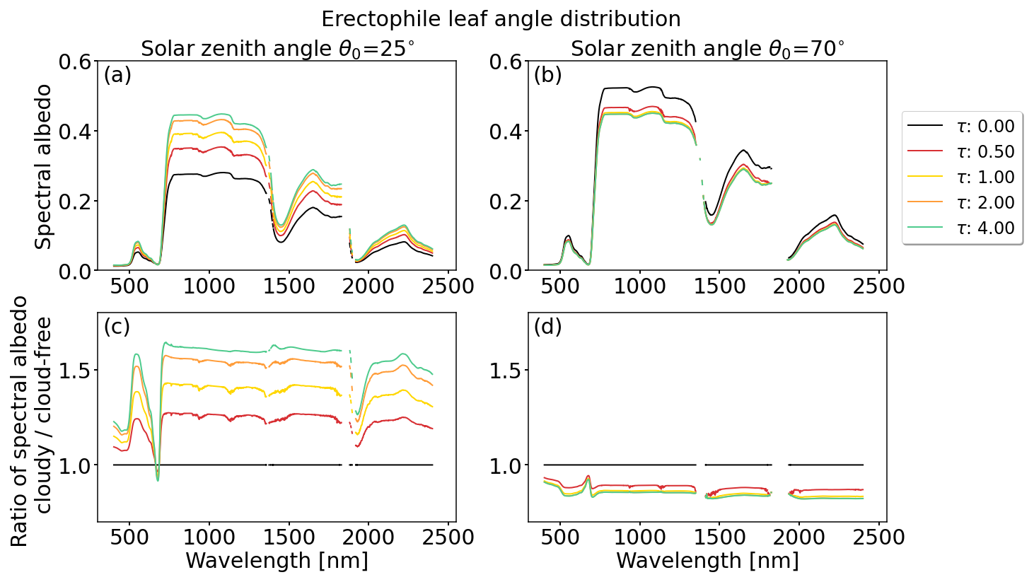
Figure 4Simulations for solar zenith angles of (a, c) θ0=25° and (b, d) θ0=70° for an erectophile leaf angle distribution and a leaf area index LAI = 3. Cloud optical thickness τ is indicated by the colored lines. From top to bottom: (a, b) spectral albedo α(λ) (unitless); (c, d) ratio (unitless) of spectral α under cloudy conditions (index c) in relation to cloud-free conditions (index cf).
Canopies with predominantly vertically oriented leaves are best described by the erectophile LAD. The vertical orientation of the leaves reduces the probability that a photon interacts with the leaves and is scattered out of the canopy (Ollinger, 2011). The lower probability of interaction inside the canopy is formalized in the vegetation extinction coefficient kext, which is lower for the erectophile than for the spherical LAD for θ0 below 52° (see right column in Table D1 and Eq. 7). In cloud-free conditions, when dominates, the deeper penetration depth also increases the probability of the radiation being absorbed by the surface. Due to the larger influence of the soil, α(λ) for θ0=25° (Fig. 4a) is generally lower compared with the spherical LAD (Fig. 3e), particularly for the cloud-free case. The narrower erectophile LAD is more sensitive to θ0 and the transition from direct to diffuse radiation. This leads to a greater variability in α(λ) under θ0=25°, compared with the spherical LAD. In cloud-free conditions, α(λ) at 850 nm is approximately 0.3 and increases to a maximum of 0.48 for τ=4. At τ=4, α(λ) approaches similar values to the spherical LAD. The increase in α(λ) from τ=0 to 4 results in a ratio of approximately 1.6, except for the absorption bands (Fig. 4c). For θ0 of 70° (Fig. 4 right column), the response of α(λ) to τ is similar to the behavior found for the spherical LAD. The generally limited response of α(λ) on τ and LAD under large θ0 is caused by the dominance of diffuse radiation, where the angular-dependent extinction of direct radiation and reflectivity in the canopy becomes negligible.
For the planophile LAD, with mostly horizontally oriented leaves, the area of each leaf and the total probability of interaction with incident radiation is largest compared with the spherical or even the erectophile distribution (Brodersen and Vogelmann, 2007; Gorton et al., 2010). Consequently, α(λ) is almost invariant with respect not only to θ0 but also to τ. For τ=6, a maximum increase of α(λ) by 2 % at a wavelength of 700 nm was determined. This is also reflected in an extinction coefficient kext, which is set to a fixed value of 1, independent of θ0 (see Table D1 and Fig. D1).
3.3 Sensitivity of broadband albedo
3.3.1 Impact of cloud optical thickness and solar zenith angle
Figure 5a, d, and g show αBB as a function of τ for the spherical, erectophile, and planophile LADs, respectively. Reading Fig. 5a, d, and g along lines of constant θ0 is interpreted as considering different cloud conditions at a fixed time on any given day. Independently of the LAD and for θ0≤60°, the broadband αBB increases with increasing τ. Within one LAD, the increase in αBB is generally largest for θ0=25°. The sensitivity of αBB on τ decreases with increasing θ0. Comparing the three LADs, the largest variability is found for the erectophile LAD, followed by the spherical LAD. For θ=25°, the transition from cloud-free to overcast conditions (τ=6) leads to an increase of αBB by 0.1 for the erectophile LAD and an increase of 0.08 for the spherical LAD. In the case of the planophile LAD, αBB is almost insensitive to τ, with an increase of about 0.002. For θ0>60°, the response of αBB is reversed for the spherical and the erectophile LAD, where αBB decreases with increasing τ. Regardless of θ0 and the LAD, αBB tends to an asymptotic value of 0.23 when τ approaches a value of 4, the incoming radiation is dominated by the diffuse component, and αBB becomes insensitive to changes in θ0 (e.g., see Fig. 3c, d). Neglecting CVRIs in the simulations, indicated by the dashed lines, results in generally lower values of αBB. The bias is of similar magnitude for all three LADs and increases with increasing τ.
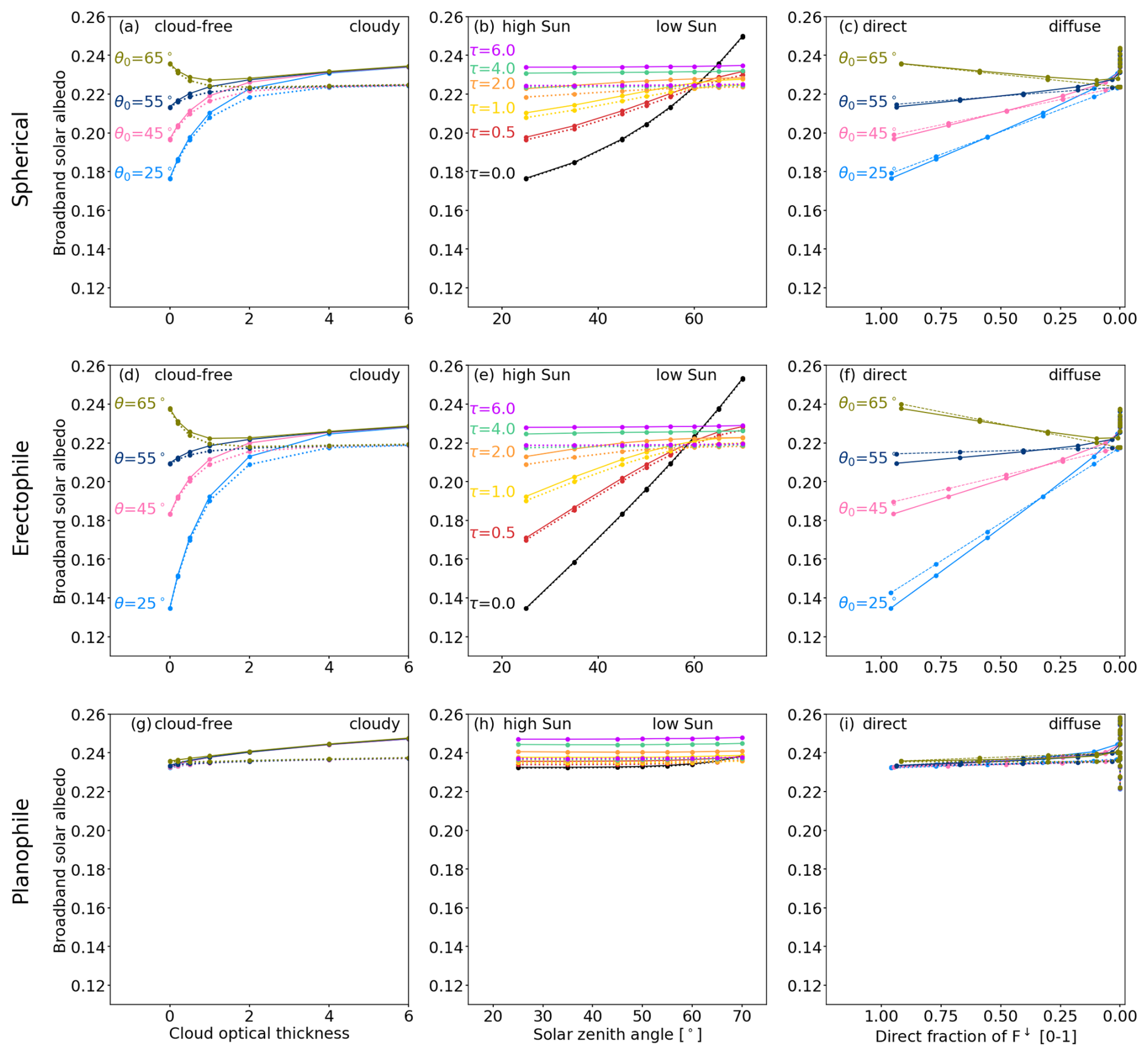
Figure 5First column: broadband solar albedo αBB,sol as a function of cloud optical thickness τ. Second column: αBB,sol as a function of solar zenith angle θ0. Third column: αBB,sol as a function of the direct fraction fdir(λ) of the downward irradiance F↓. Lines along θ0 and τ are color-coded. Columns from top to bottom provide αBB based on the spherical, erectophile, and planophile leaf angle distribution, respectively. The dashed lines in the first and second column represent αBB obtained for uncoupled simulations that neglect cloud–vegetation–radiation interactions. The dashed lines in the third column represent parameterized αBB.
Figure 5b, e, and h show the dependence of αBB on θ0 for constant τ. The response of αBB along the lines of constant τ represents the diurnal cycle of the Sun under constant cloud conditions. In the case of the spherical and erectophile LAD, an increase in θ0 is associated with an increase in αBB. The change in αBB is largest for cloud-free conditions (τ=0), being most pronounced for the erectophile LAD, and followed by the spherical LAD. This is due to the angular dependence of scattering in the canopy, which is more pronounced for the erectophile than for the planophile LAD (see Appendix Fig. D1). For τ=0, the transition from θ0=25° to 70° leads to an increase in αBB by 0.12 for the erectophile LAD and an increase of 0.09 for the spherical LAD, which is similar in magnitude compared with the change of τ for constant θ0=25. For increasing τ, the sensitivity of αBB to θ0 is progressively reduced until αBB becomes insensitive to θ0 for τ=6. As for the sensitivity of αBB to τ, for an overcast sky that is dominated by diffuse radiation, αBB becomes insensitive to the angular-dependent extinction of the radiation in the canopy, and thus the Sun's diurnal cycle becomes less influential on αBB. In the case of the planophile LAD, αBB is almost insensitive to θ0, irrespective of the actual value of τ.
Figure 5c, f, and i show the relationship of αBB on fdir(λ), which itself depends on τ and θ0. Plotting fdir(λ) instead of τ or θ0 removes potential ambiguities, since multiple combinations of τ and θ0 can lead to the same value of fdir(λ). Furthermore, it removes the exponential relationship of Eq. (7). Moving along lines of constant θ0 is then synonymous with a change in τ. For the spherical and erectophile LADs, in combination with θ0<60°, αBB increases with decreasing fdir(λ), while for 60° the opposite effect appears. The transition from only direct radiation to only diffuse radiation has the greatest effect for θ0=25° and decreases with increasing θ0. For the spherical and erectophile LADs, the lines of constant θ0 converge and approach an asymptotic value, indicating that the angular sensitivity of αBB on θ0 disappears with increasing cloudiness. The planophile LAD is generally insensitive to changes in fdir(λ), regardless of θ0.
3.3.2 Impact of leaf area index
The LAI is an important parameter that describes the optical properties of a canopy. The simulations in this paper use the SCOPE2.0 default value of 3. Additional simulations with LAIs from 1 to 5 are performed for all three LADs to account for different canopy types, the annual vegetation cycle, and potential leaf loss, for example due to drought. Figure 6 shows the response of αBB to LAI under cloudy conditions with τ=0.5 for the erectophile LAD. Since the LAI describes the leaf area per unit surface area, an increase in the LAI results in a higher probability of incident radiation interacting with the leaves. This is represented in the simulations where αBB increases with increasing LAI. However, the response of spectral α(λ) to changes in LAI is strongly wavelength-dependent, and the broadband αBB is a superposition of two opposing contributions. While for wavelengths greater than 700 nm an increase in LAI leads to an increase in spectral α(λ), because vegetation typically has higher albedo values than bare soil in this wavelength range, an increase in LAI results in a decrease in spectral α(λ) for shorter wavelengths, because in this wavelength range the albedo of vegetation is lower than the albedo of dry bare soil (Yang et al., 2021). The response of αBB to LAI under different values of θ0 can be explained by the vegetation extinction coefficient kext(θ,λ), which itself depends on wavelength, LAD, and incident angle θ (Bréda, 2003). The first-order approximation of kext(θ,λ) given in Fig. D2 and in Appendix D shows that, for the same LAD, the extinction of radiation depends more strongly on LAI when θ0 is large. This explains the higher sensitivity of αBB to changes in LAI for larger values of θ0. Figure D2 also shows that, for constant LAI, the difference in kext(θ,λ) caused by a variation in θ0 is more pronounced for the erectophile LAD, followed by the spherical and planophile LADs. This explains why the lines of constant θ0 are well separated for the erectophile LAD shown in Fig. 6, while the lines of constant θ0 are closer together for the spherical LAD and almost identical for the planophile LAD (both not shown here). Regardless of the LAD, the relationship between LAI and αBB is generally non-linear. Because of the increasing overlap of leaves with increasing LAI, the increase in additional leaf area does not contribute linearly to the illuminated leaf area that can scatter and absorb incoming radiation.
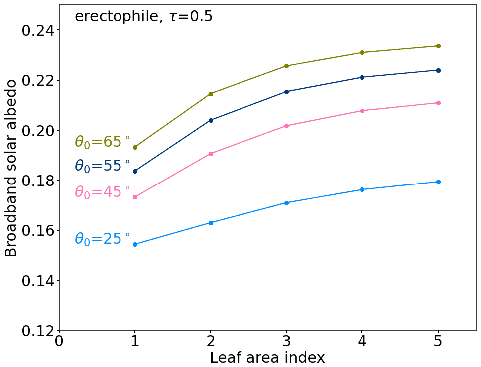
Figure 6Above-canopy broadband solar albedo αbb as a function of leaf area index for an erectophile leaf angle distribution and a cloud optical thickness τ=0.5.
3.4 Separation of coupling effects
3.4.1 Contribution of multiple scattering to the enhancement of vegetation albedo
Cloud–vegetation–radiation interactions, here primarily multiple scattering between cloud base and the canopy, are known to enhance the observed spectral albedo (Weihs et al., 2001; Wendisch et al., 2004; Gueymard, 2017). The enhancement is caused by an additional contribution of radiation to that was reflected at the TOC back to the atmosphere and again back to the canopy by the cloud base (Freedman et al., 2001; Min and Wang, 2008; Kanniah et al., 2012; Gueymard, 2017). The relative contribution of CVRIs to the total F↓(λ), expressed as ξ(λ), is estimated by
where represents simulated downward irradiance under cloudy conditions from uncoupled (index “uc”) simulations and represents simulated downward irradiance under the same cloud conditions but from the coupled (index “co”) simulations.
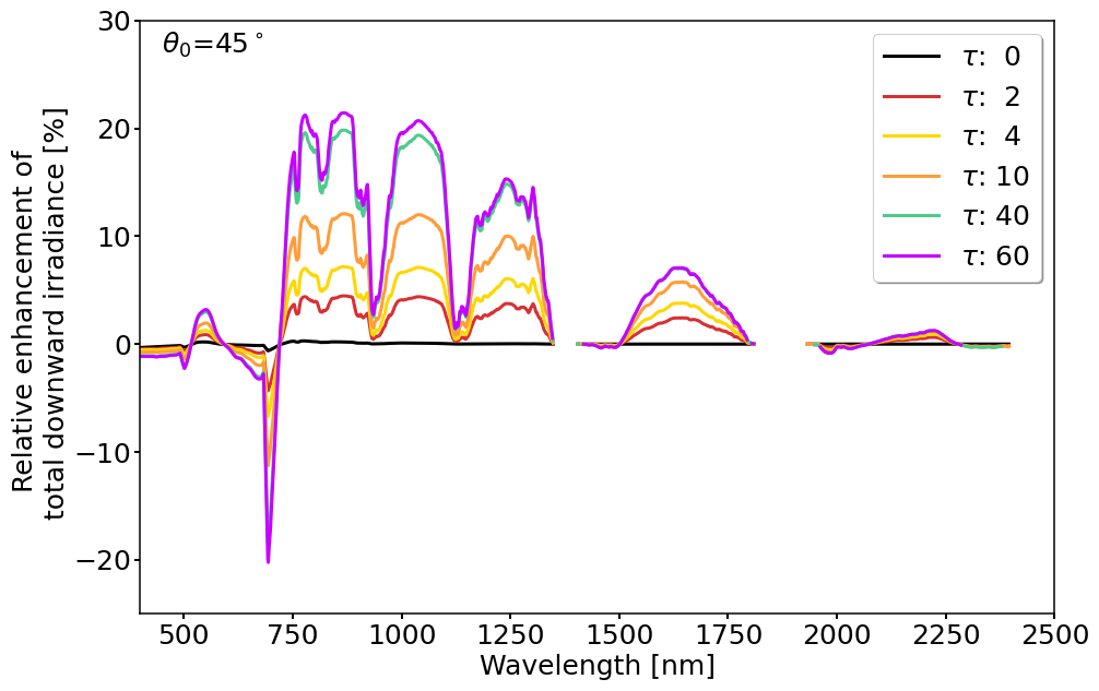
Figure 7Relative contribution of ξ(λ) (as a percentage) of downward diffuse irradiance to the enhancement of spectral albedo α(λ) due to multiple scattering. An intermediate solar zenith angle θ0 of 45° was selected. Six cloud conditions were considered, with cloud optical thickness τ (unitless) ranging between 0 and 60.
Figure 7 shows that ξ(λ) is largest for wavelengths between 750 and 900 nm, where α(λ) and F↓(λ) are characterized by their largest values. Exceptions are the water-vapor absorption bands and the red edge at a wavelength of about 700 nm. In cloud-free cases (τ=0, black line), with scattering from molecules and aerosols only, ξ(λ) is negligible, with a maximum of about ±0.2 % at 750 nm. With increasing values of τ, which yield more diffuse radiation and a more reflective cloud base, ξ(λ) increases continuously at wavelengths of about 600 nm and for all wavelengths greater than 750 nm. The identified influence of multiple scattering on the surface albedo agrees with earlier observations by Parisi et al. (2003), who identified enhanced diffuse ultraviolet radiation at the surface under cloudy conditions, compared with cloud-free conditions. As shown here, similar effects also occur for longer wavelengths in the visible–near infrared spectra, particularly where α(λ) convoluted with F↓(λ) is large. Generally, all cases with high surface albedo, i.e., over snow- and ice-covered areas, are prone to enhanced diffuse radiation and albedo below clouds (Hay, 1976; Kierkus and Colborne, 1989; Gueymard and Ruiz-Arias, 2016; Gueymard, 2017). Since vegetation albedo is lower than ice- and snow-covered surfaces, the effects above vegetation are less pronounced. Since ξ(λ) represents the relative contribution to F↓(λ), the absolute downward F↓(λ) is still decreasing with increasing τ. Thus, ξ(λ) is driven by the superposition of α(λ) and F↓(λ) is visible in the spectral slope and the general decrease of ξ(λ) with wavelength.
3.4.2 Separating the directional and spectral effects by the downward radiation
In Sect. 3.3 it is shown that fdir(λ) is the main parameter controlling αBB. The individual contributions of direct and diffuse F↓(λ) to changes in αBB are quantified by simulating hypothetical cases with either direct or diffuse components of F↓(λ). The albedo driven by only direct radiation is commonly referred to as the black-sky albedo, while the albedo that is driven by only diffuse radiation is referred to as the white-sky albedo. The black-sky and white-sky albedos are extreme cases and the actual albedo observed in nature is called blue-sky albedo, which is an intermediate condition between the two extreme cases (Lucht et al., 2000). Figure 8a–c show αBB as a function of τ for the spherical LAD and three values of θ0: 25, 50, and 70°, respectively. In each panel, the given blue-sky albedo is identical to the graphs given in Fig. 5a. For values of θ0 of 25 and 50°, αBB is lowest for the black-sky albedo, while the highest values of αBB are found for the white-sky albedo. The black-sky and white-sky albedos increase with increasing τ. The blue-sky albedo, as an intermediate condition between the black-sky and white-sky albedos, is closest to the black-sky albedo for cloud-free conditions and approaches the white-sky albedo under overcast conditions (τ>6). This agrees with the observations of Freedman et al. (2001) and Kanniah et al. (2012), who found an increase in the canopy albedo under cloudy conditions compared with clear-sky conditions. The different slopes of the blue-sky albedo for different values of θ0 are caused by the different penetration depths of direct radiation into the canopy. For small values of θ0 and a dominating direct radiation, the penetration depth into the canopy is high and radiation is more likely to be absorbed, resulting in a lower αBB. Consequently, the difference with respect to the white-sky albedo is greater for θ0=25° (Fig. 8a), compared with θ0=50° (Fig. 8b). For even larger values of θ0=70°, increasing τ results in a decrease of αBB.
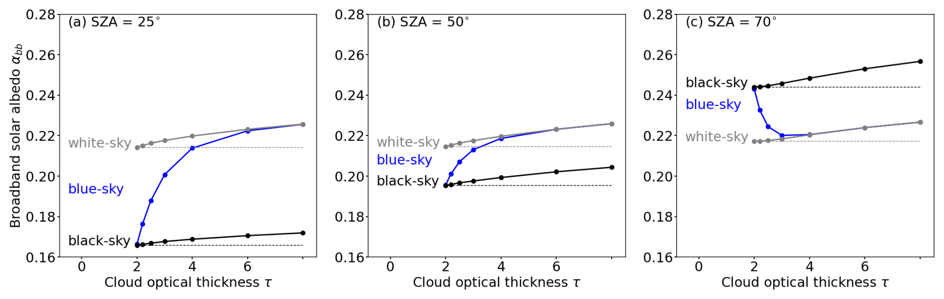
Figure 8(a–c) Broadband solar albedo αBB as a function of cloud optical thickness τ for three solar zenith angles θ0: (a) 25°, (b) 50°, and (c) 70°. Simulations are performed for a spherical leaf angle distribution and a leaf area index of 3 m2 m−2. Simulations including the direct and diffuse fraction of F↓ (blue-sky albedo) are given in blue. Simulations including only the direct fraction of F↓ (black-sky albedo) are given in black, while broadband albedo including only the diffuse fraction of F↓ (white-sky albedo) are given in gray. The dashed lines provide a reference for black-sky and blue-sky albedos.
Broadband αBB is also modified by spectrally dependent scattering and absorption by clouds that shifts the weighting of α(λ) with F↓(λ) from longer to shorter wavelengths. These effects are shown for the black-sky and white-sky albedos with respect to the cloud-free state with τ=0 (dashed lines as reference). For θ0=25°, the black-sky albedo increases by 0.005 and the white-sky albedo increases by 0.06 at τ=8, compared with the reference at τ=0. For a value of θ0 of 70°, the black-sky albedo increases by 0.06 and the white-sky albedo increases by 0.07 at τ=8, compared with the reference at τ=0. Regardless of θ0, the shift in the weighting of α(λ) to shorter wavelengths enhances the black-sky, white-sky, and blue-sky albedos, but the enhancement is relatively small compared with the overall increase in blue-sky albedo caused by the change in fdir. The effect is small because the weighting is shifted to the wavelength range in which vegetation has the lowest albedo. However, it should be noted that the relative importance of the wavelength shift increases with τ as the absolute difference between black-sky and white-sky albedo decreases with increasing θ0. Furthermore, the effect of the wavelength shift remains effective even when fdir=0 and diffuse scattering already dominates (see Fig. A1 in the Appendix).
3.5 Consequences for calculating the cloud radiative effect
3.5.1 Effect of neglected cloud–vegetation–radiation interactions
Within the ECMWF IFS, the vegetation albedo is based on monthly climatologies of LAI and vegetation type, and thus indirectly on the LAD (ECMWF, 2021). No separation between black-sky and blue-sky albedos is made (ECMWF, 2021). Consequently, neither the influence of clouds on vegetation albedo nor that of CVRIs is considered in RT simulations performed within the ECMWF IFS or models with similar albedo implementation. Three cases were employed to quantify the differences in the solar radiative energy budget at the top of the canopy resulting from neglecting CVRIs and assuming a constant cloud-free vegetation albedo.
-
Case A. Neglecting the cloud-induced albedo and CVRIs represents the current albedo implementation of the vegetation ECMWF IFS, where the vegetation albedo is set to a constant value. The resulting radiative effect is quantified by the solar radiative forcing ΔF at the canopy level between the downward broadband irradiance obtained from coupled simulations (index “co”), including the actual cloud-induced albedo αBB,co(τ), and the downward broadband irradiance obtained from uncoupled simulations (index “uc”) with a fixed cloud-free albedo . The solar radiative forcing ΔF is formalized by
-
Case B. Neglecting CVRIs but accounting for the cloud-induced albedo causes a radiative effect that is quantified by the solar CVRI forcing ΔFcvri, calculated at the canopy level between from coupled simulations and from uncoupled simulations, both accounting for the actual cloud-induced albedo. The CVRI forcing ΔFcvri is formalized by
-
Case C. Neglecting the cloud-induced albedo but including CVRIs introduces a bias, which we call the solar albedo forcing ΔFalb. It is quantified at the canopy level between combined with the cloud-induced albedo αBB,uc(τ) and combined with a fixed cloud-free albedo αBB(τ=0). The albedo forcing ΔFalb is estimated from uncoupled simulations, since coupled simulations would include CVRI effects. The solar albedo forcing ΔFalb is formalized by
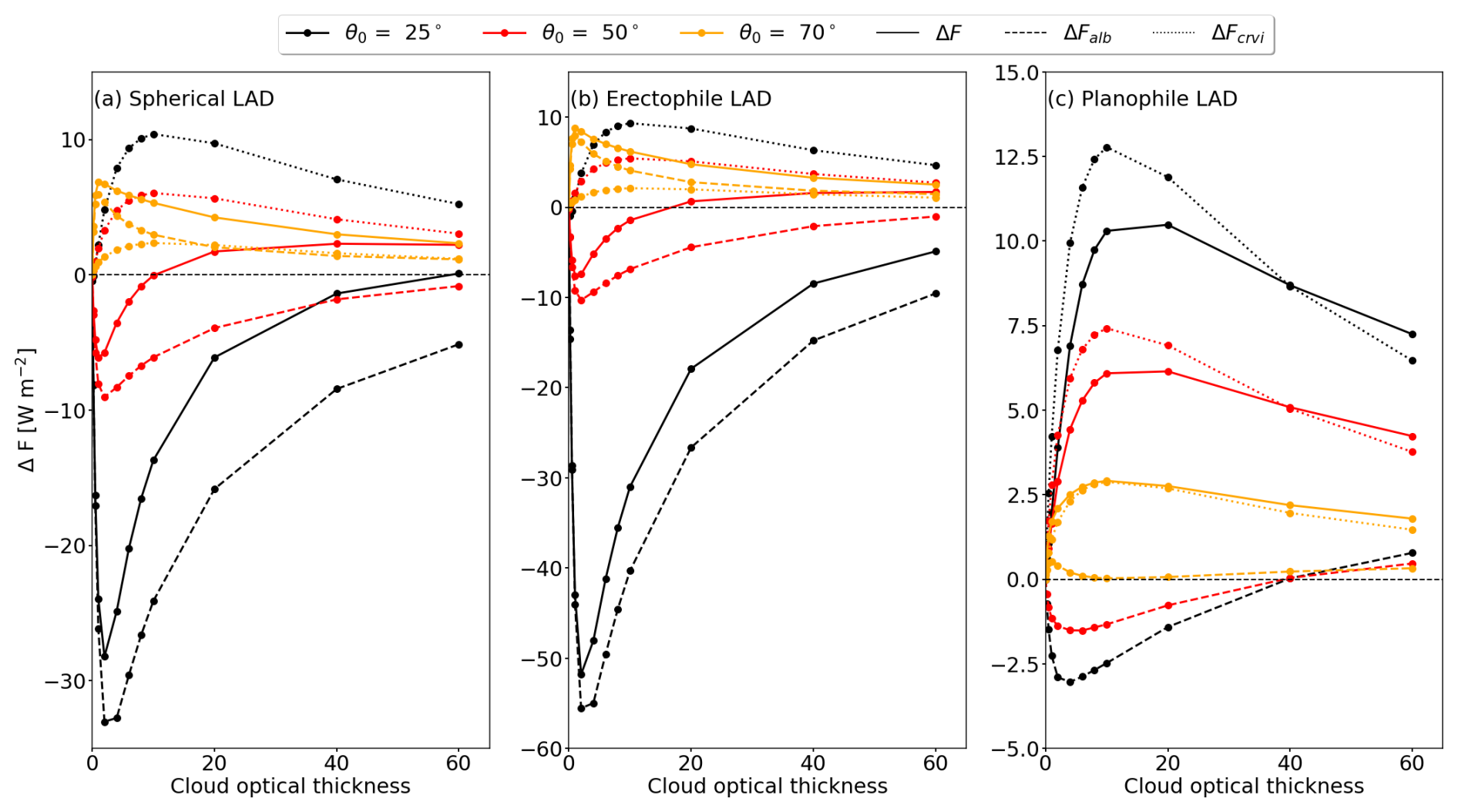
Figure 9Absolute difference in above-canopy broadband solar albedo forcing ΔFalb (dashed line), broadband solar CVRI forcing ΔFcvri (dotted line), and resulting broadband solar forcing ΔF (solid line) due to the cloud-modulated canopy albedo and multiple-scattering effects. Results are given for (a) spherical, (b) erectophile, and (c) planophile leaf angle distributions, and three solar zenith angles, θ0: 25, 50, and 70°.
Figure 9a shows ΔF, ΔFalb, and ΔFcvri for a spherical LAD. For θ0 less than 60°, ΔFalb increases with increasing τ, reaches a maximum, and then decreases for further increases in τ. For θ0<60°, the cloud-induced αBB is greater than the αBB under cloud-free conditions, causing the first term in Eq. (12) to be greater than the second term, resulting in negative ΔFalb. A peak value of ΔFalb 35 W m−2 occurred for the combination of θ0=25° and τ=4. For values of θ0 of 50 and 70°, peak values of −8 and 6 W m−2 were determined, respectively. Positive values of ΔFalb result from the decrease of αBB when transitioning from clear-sky to cloud-induced αBB (see Fig. 5a). Independently of θ0, further increasing τ beyond the respective peak values of ΔFalb leads to a decrease in ΔFalb, which is caused by a decrease in that counterbalances the effect of the cloud-induced albedo.
Independently of the Sun's position, the contribution of the CVRIs leads to positive ΔFcvri, reaching peak values up to 10 W m−2 for the combination of τ=6 and θ0=25°. The CVRI forcing is positive because and the cloud-induced αBB are larger for the coupled simulations (first term in Eq. 11) than for the uncoupled simulations (second term in Eq. 11). As for ΔFcvri, a further increase of τ beyond the maxima of ΔFcvri, leads to a decrease due to the decrease in with τ.
The greatest forcing is related to ΔF, which can be partly understood as a superposition of ΔFalb and ΔFcvri. The solar forcing can be positive or negative depending on the combination of θ0 and τ. It is noted that , since different stages of the coupling are used in the calculation of ΔFalb and ΔFcvri. For small values of θ0=25° and optically thin clouds, ΔF is negative with values up to −28 W m−2 at τ=6, becomes smaller with increasing τ, and changes sign for optically thick clouds at τ=60 due to the dominance of ΔFcvri. For greater θ0, of about 50°, ΔF approaches a peak value of −7 W m−2 at τ=6, and becomes positive for τ≈15. For θ0=70°, ΔF is positive for all values of τ.
For the erectophile LAD, a similar behavior of ΔF to τ is observed, but with greater magnitude in ΔFalb and ΔF, resulting in peak ΔF of −52 W m−2 for θ=25° and 10 W m−2 for θ=70°. Compared with a canopy with a spherical LAD, an erectophile canopy generally has a lower reflectivity, resulting in reduced multiple scattering between TOC and the cloud base. This leads to lower ΔFcvri for all values of θ0.
The planophile LAD, with preferentially horizontally oriented leaves, reflects a larger fraction of the incoming radiation that can contribute to the enhancement of F↓ below clouds, resulting in the largest values of ΔFcvri among all three LADs (Brodersen and Vogelmann, 2007; Gorton et al., 2010). The albedo forcing associated with the planophile LAD was found to be the smallest, not exceeding −2.6 W m−2 for θ0=25°, since αBB is almost insensitive to changes in τ (see Fig. 5g–i). Overall, ΔF is dominated by positive ΔFcvri, resulting in positive ΔF for all simulated conditions of θ0 and τ.
Regardless of the solar zenith angle, ΔFalb, ΔFcvri, and ΔF are most sensitive and reach peak values in the simulated cases when τ is less than 20. This results from the sensitivity of αBB and fdir to τ<6 and the non-linear behavior of , which has a maximum at about τ=4–6 below liquid water clouds (Bohren, 1987). Therefore, the transition from cloud-free to cloudy conditions with τ<20 is most susceptible to biases, when neglecting the diffuse vegetation albedo and CVRIs.
Neglecting CVRIs and the influence of clouds on the vegetation albedo introduces biases in the surface radiation budget. As shown in Fig. 9, neglecting CVRIs underestimates the amount of diffuse radiation between canopy and cloud base under illumination conditions with θ0<60°. This is explained by the relatively small extinction coefficient for θ0<60°, allowing direct radiation to penetrate deep into the canopy and to be absorbed by the canopy or soil, where it is converted into latent and sensible heat. Both fluxes are known to be important for boundary layer processes and local cloud formation (Freedman et al., 2001; Bosman et al., 2019). In contrast, a generally higher fdir below clouds and CVRIs increases the probability that radiation is reflected in the upper parts of the canopy and lowers the probability of absorption by the understory or soil. A second potential consequence of neglecting CVRIs is an incorrect estimate of the radiation available for photosynthesis. Due to the presence of clouds, the radiation reflected at the top of the canopy is again reflected at the cloud base that is available as diffuse radiation. It is known that diffuse radiation below optically thin clouds with τ≤6 increases the amount of photosynthetically active radiation, since diffuse radiation can penetrate deeper into the canopy and all parts of the leaves can absorb radiation, not only the leaf areas illuminated by direct radiation (Freedman et al., 2001; Min and Wang, 2008; Kanniah et al., 2012; Cheng et al., 2016). In the same manner, the enhancement of diffuse radiation by CVRIs potentially increases photosynthesis rates that would be underestimated otherwise. This results in a potential underestimation of plant productivity and carbon uptake (Freedman et al., 2001).
3.5.2 Parameterization of the cloud effect on broadband surface albedo
To better approximate the effect of clouds on the vegetation albedo, we propose a parameterization of αBB as a function of broadband fdir to account for CVRIs and the cloud-induced vegetation albedo (Fig. 5). The parameterization takes atmospheric parameters θ0 and fdir and the vegetation parameters LAI and LAD as input. The parameterization of αBB is formalized by
where μ=cos (θ0) and g(μ) is given by
The parameters a1 to a4 and b1 to b3 for the spherical, erectophile, and planophile LADs are provided in Table 3.
Table 3Parameters and polynomials for the parameterized broadband solar albedo αBB. Maximal deviations ΔαBB between simulation and parameterization.
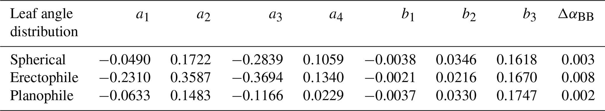
The parameterization of αBB is evaluated against the simulated values of αBB and is overlaid in the right column of Fig. 5. The values of αBB from the simulations and the parameterization mostly overlap, indicating a good agreement of the parameterization with the simulations. Regardless of the LAD, discrepancies appear, mainly when fdir approaches a value of 0. In general, the largest differences appear for the erectophile LAD, but remain below a value of ΔαBB=0.005, which corresponds to a relative error of 2.3 % with respect to αBB=0.22. Since the proposed parameterization takes fdir as input, the parameterization only accounts for the transition from direct to diffuse radiation, i.e., the transition from cloud-free to the cloud-induced αBB. The shift in the spectral weighting, which persists even when fdir=0, is not considered. However, the contribution of the wavelength shift is generally small compared with the effect of fdir, as shown in Fig. 8 and Appendix A.
3.6 Limitations of the simulations
libRadtran and SCOPE2.0 allow for the specification of a variety of parameters during the simulation set-up. While certain parameters, such as θ0, τ, LAI, or LAD, were varied in the present study, other parameters were left at their respective model defaults from libRadtran (Sect. 2.2.1) and SCOPE2.0 (Sect. 2.2.2). Since this idealized set-up does not cover the natural variability of atmospheric and vegetation conditions, the chosen default values may affect the results presented in this study. An additional sensitivity analysis of selected default parameters, which potentially impact the RT in the solar wavelength range, was performed. Details about the sensitivity analysis, the varied parameters, and the value ranges are provided in Appendix C. It is noted that the sensitivity study does not cover all possible parameters in both models and is therefore not comprehensive. It should be regarded as a first-order approximation of potential uncertainties associated with the fixed parameters, providing an estimate for the robustness of the presented results.
Within the varied atmospheric parameters, the variation of the vertical temperature and relative humidity profile showed the largest impact on αBB, with an increase of up to +0.01, when the mid-latitude summer profile (“afglms”, default) was replaced with the mid-latitude winter profile (“afglmw” Anderson et al. (1986)). Effects of aerosol concentration, cloud altitude, and cloud droplet size were found to be of minor importance, with a variation in αBB below ±0.008. Among the varied vegetation parameters, the largest effect on αBB was found for plant dry matter. Varying the plant dry matter by ±25 % around its default value of 0.0012 g cm−2 resulted in a variation in αBB of ±0.013, which is of a similar magnitude to that obtained with a change in the LAI from 2 to 3. The second most influential factor in the sensitivity analysis was the leaf structure parameter, which is known to be an uncertainty factor in vegetation RT and modeling (Boren et al., 2019). However, the variation of αBB due to changes in the leaf structure parameter is smaller than the effects reported from changes in τ and θ0. Variations in chlorophyll a and b content, carotenoid content, leaf water equivalent layer, the model parameter for soil brightness, and the volumetric soil moisture content in the root zone resulted in absolute deviations in αBB of ±0.003 maximum. Neither the present study nor the sensitivity analysis considered the influence of canopy structure. Canopy structure is known to be a key factor in determining the amount of radiation that is absorbed, reflected, and transmitted in a canopy (Ni-Meister et al., 2010). For example, clumping reduces the sunlit area of the leaf ensemble compared with randomly oriented leaves for the same LAI. This affects the interaction of incoming radiation and consequently the canopy albedo (Ni and Woodcock, 2000; Chen et al., 2008). All simulations performed are based on the assumption of a homogeneous canopy to cover a wider range of canopy types, since clumping depends on vegetation type, among other factors. By not accounting for leaf clumping, the amount of radiation absorbed by the sunlit leaf area is overestimated (Li et al., 2023) and neglecting clumping in our simulations may reduce the dependence on θ0 and τ in our simulations (Kanniah et al., 2012; Li et al., 2023).
This study investigated cloud–vegetation–radiation interactions (CVRIs) by coupling an atmospheric radiative transfer (RT) model, the library for Radiative Transfer (libRadtran), and a vegetation RT model, the Soil Canopy Observation of Photosynthesis and Energy fluxes (SCOPE2.0). This goes beyond previous model set-ups, where vegetation RT models neglected the influence of clouds, which are now explicitly included in the coupled radiative transfer simulations.
The coupled simulations were run for an interval of solar zenith angles θ0 ranging from 25 to 70°. A stratiform liquid water cloud was simulated with cloud optical thickness τ ranging from 0, for cloud-free conditions, to 80, for fully overcast conditions. The range of τ is intended to represent a typical mid-latitude spring, summer, or autumn day. The diversity of plant characteristics was attempted to be partly represented by spherical, erectophile, and planophile leaf angle distributions (LADs), and variations of the leaf area index (LAI) between 1 and 5 m2 m−2 (inclusive). The simulations by libRadtran and SCOPE2.0 covered a wavelength range from 0.4 to 2.4 µm. The iterative coupling was realized by initializing SCOPE2.0 with the spectral, downward direct , and diffuse irradiance provided by libRadtran. libRadtran was initialized with a first guess vegetation albedo, which was replaced in the next iteration step with the vegetation albedo provided by SCOPE2.0. Two cycles were found to be sufficient for the iteration to converge.
The iterative coupling allowed the change in the direct fraction under cloudy conditions and CVRIs to be accounted for in the calculation of the cloud-induced vegetation albedo. An example case showed that initializing SCOPE2.0 with direct and diffuse downward irradiance under cloudy conditions enhanced the spectral vegetation albedo α(λ) by about 10 % to 15 % compared with cloud-free conditions. The inclusion of CVRIs resulted in a further increase of about 1 % to 5 %. The enhancement was found to be wavelength-dependent, with the largest relative differences near the water-vapor absorption bands and where high values of α(λ) and total downward irradiance F↓(λ) coincide.
Based on the varied parameters and parameter ranges, it was found that the LAD is the primary factor controlling the sensitivity of αBB to LAI, θ0, and τ. Assuming an erectophile LAD in the simulations, αBB was most sensitive to the varied parameters, especially for combinations of small τ<6 and small θ0<50°, i.e., large values of the direct fraction fdir(λ). Generally, lower sensitivities of spectral and broadband α to τ and θ0 were found for the spherical LAD. Spectral and broadband α of the planophile LAD were found to be almost insensitive to τ and θ0 for the same parameter ranges. The sensitivity of α(λ) to LAI, LAD, and θ0 decreased continuously with decreasing fraction fdir(λ) because the incident radiation becomes more diffuse, i.e., undirected, and the angular-dependent scattering in the canopy becomes insensitive to the canopy structure given by LAI and LAD. The second effect that affected the spectrally integrated broadband albedo αBB was the wavelength-dependent absorption and scattering by clouds, which shifted the weight of the incoming radiation toward shorter wavelengths. Due to the generally low values of α(λ) below 700 nm, the effect of the wavelength shift was found to be small in absolute values, increasing αBB by up to 0.07 (θ0=70° and τ=6). In summary, the change in fdir(λ) was found to be relevant for values of τ between 0 and 6, when direction radiation is dominant. Beyond τ of 6, the shift in the spectral weighting of α(λ) with F↓(λ) was found to be the main contributor to changes in αBB.
Different stages of the iterative process were used to separate the effects of diffuse radiation on α(λ) from the effects of multiple scattering. Iterative coupling was found to be particularly important to account for multiple scattering between the top of the canopy and the cloud base, which enhanced by up to 22 % at wavelengths between 750 and 900 nm for a cloud with cloud optical thickness τ=60.
The radiative effect of clouds on αBB and the resulting radiation budget below clouds was estimated in terms of the solar forcing ΔF at the top of the canopy. The solar forcing ΔF was determined between uncoupled simulations that neglected the influence of clouds on vegetation albedo and coupled simulations that included the cloud effects on vegetation albedo. The solar forcing was further decomposed into the solar albedo forcing ΔFalb, representing the bias due to a fixed vegetation albedo, and the solar CVRI forcing ΔFcvri, representing the bias by missing CVRI. The greatest sensitivity of ΔF was found for the transition from cloud-free to cloudy conditions (τ<6). The largest absolute values of ΔF were identified for θ0=25°, leading to negative ΔF of up to −58 W m−2, implying a stronger reflection by vegetation in the coupled simulations, compared with uncoupled simulations that neglected the influence of clouds. The maximum values of ΔF decreased with increasing θ0 and also reversed sign, so that for θ0=70°, ΔF became positive, with values up to 8 W m−2. The contributions of ΔFalb and ΔFcvri to ΔF were found to depend on the combination of LAD, θ0, and τ since both components can have opposite signs. For the spherical and erectophile LAD, ΔFalb dominated in most cases, while for the planophile LAD, ΔFcvri dominated ΔF.
The nearly linear correlation between αBB and fdir has been exploited to parameterize the effect of clouds on αBB over vegetated areas. The parameterization accounts for θ, LAI, LAD, and fdir. It has been shown that the parameterization is able to reproduce the simulated cloud-induced albedo changes with a relative error of less than 2.4 %. The approach to parameterize the effect of clouds on αBB over vegetated areas may be suitable for implementation in numerical weather prediction or global circulation models to improve the surface radiation budget over vegetated areas under cloudy conditions.
The idealized simulation set-up and the multitude of vegetation parameters did not enable coverage of the natural variability of atmospheric and vegetation conditions, and the chosen default values may affect the results presented in this study. A sensitivity study was performed to estimate the influence of these default parameters and to test the robustness of the results. Among the varied parameters, plant dry matter had the largest effect on αBB, followed by the assumed atmospheric profile and the leaf structure parameter. Varying the default values by ±25 % caused deviations in αBB of up to ±0.013, which corresponds to a change in LAI of about 1. Variations in aerosol visibility, cloud altitude, and cloud droplet effective radius contributed only little. Variations in chlorophyll a and b content, carotenoid content, leaf water equivalent layer, the BSM model parameter for soil brightness, and the volumetric soil moisture content in the root zone had only small effects. It is further acknowledged that the simulations assume a homogeneous canopy and that structural effects, such as leaf clumping, were not considered in this study. However, these structural effects operate on a local scale and are likely to be smoothed out, given the current spatial resolution of numerical weather prediction models and global circulation models.
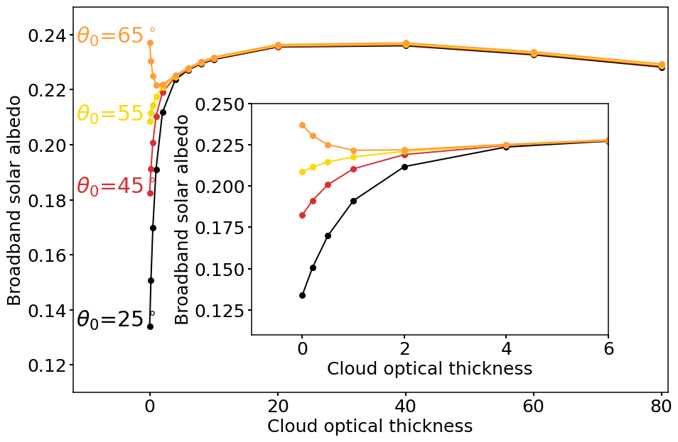
Figure A1Above-canopy broadband solar albedo αbb as a function of cloud optical thickness τ ranging from 0 to 80 and for four solar zenith angles, with a default leaf area index of 3. An erectophile leaf angle distribution is assumed.
Coupled simulations of spectral irradiance F(λ) and albedo α(λ) have been performed for cloud optical thickness τ with values between 0 and 80. Integration of α(λ) using Eq. (5) gives the broadband αBB weighted by the incoming F↓(λ). Spectral-dependent scattering and absorption by clouds shifts the relative weighting toward shorter wavelengths. Figure A1 shows the response of αBB on τ for the erectophile leaf angle distribution (LAD). Initially, αBB increases or decreases with increasing τ until the diffuse component of F↓(λ) dominates at τ=6. This increase is related to the transition from only direct (τ=0) to diffuse (τ=6) downward irradiance F↓(λ). Beyond a value of τ=6, the further increase of αBB is only related to the shift of the weighting in F↓(λ) to shorter wavelengths. The spectral slope of the incoming radiation – roughly decreasing with increasing wavelength – and the spectral slope of the vegetation – low α(λ) below 700 nm, steep increase, and decreasing with increasing wavelength – lead to a maximum in the convolution of α(λ) and F↓(λ), such that αBB becomes maximal at τ≈20. Beyond this optimum, αBB decreases because the spectral weighting in F↓(λ) is shifted more and more into the spectral range where the radiation is almost completely absorbed by vegetation. The simulation with the erectophile LAD represents an extreme case. For the spherical and planophile LADs, a reduced sensitivity of αBB to τ between 0 and 6 was found. However, the position of the maximum at around τ=20 was shown to be insensitive to the selected LAD.
Radiation passing through the atmosphere is scattered and absorbed by aerosol particles, gas molecules, and clouds. The influence of clouds on the direct irradiance and the diffuse irradiance components of the total irradiance F↓(λ) is shown in Fig. B1 for an intermediate solar zenith angle θ0 of 45°.
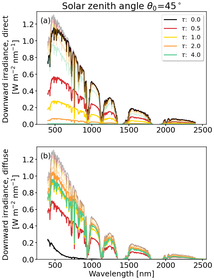
Figure B1(a) Spectral, downward, direct irradiance; (b) diffuse irradiance. In both panels, spectral, downward, total irradiance F↓(λ) is underlaid by faded lines. Cloud optical thickness τ is indicated by the colored lines. Simulations are based on a spherical leaf angle distribution for a solar zenith angle of θ0=45°.
All spectra are characterized by water-vapor absorption bands at wavelengths of 933–946, 1118–1144, 1350–1480, and 1810–1959 nm due to molecular absorption. An increase in τ results in a decrease in (Fig. B1a). Wavelengths below 900 nm that are outside of the absorption bands are primarily affected by Rayleigh and Mie scattering (Mie, 1908), leading to a flattening of the spectrum below 500 nm. Wavelengths above 900 nm and within the water-vapor absorption bands are dominated by absorption. It is further noted that, with decreasing/increasing θ0, the path of the radiation through the atmosphere and the cloud becomes shorter/longer, leading to fewer/more scattering processes. Consequently, the same values of cloud optical thickness τ yield values of that are greater/less for θ0 less/greater than θ0=45°. Radiation scattered at least once by atmospheric constituents is removed from the direct component and contributes to the diffuse component given in Fig. B1b. For the cloud-free case (black), is close to zero except for wavelengths λ<750 nm due to Rayleigh scattering. Regardless of θ0, including clouds in the simulations leads to an overall increase in . However, the increase is not continuous and reaches maximum values for τ between 2 and 4 at θ0=25° and for τ around 1 at θ0=75°. This is a result of the pronounced forward peak in the scattering phase function of water droplets, which enhances scattering toward the surface compared with cloud-free conditions. According to Bohren (1987), the maximum value of occurs under cloudy conditions when , where g is the asymmetry factor, with a representative value of g=0.85 for clouds in the visible–near infrared wavelength range (Irvine and Pollack, 1968).
To investigate the robustness and potential uncertainties of the broadband surface albedo αBB to variations of the input parameters that were previously fixed in the study, an additional sensitivity study was performed. All simulated combinations were based on an intermediate solar zenith angle θ0=45° and a cloud optical thickness τ=4, which were chosen to represent mean illumination conditions that were targeted in the present paper.
Table C1 lists all parameters that were kept previously constant but were varied in the sensitivity study. Table C1 also lists the default values and the absolute values that resulted from a variation by ±25 % from their default value. While this may not cover the full range of possible parameters, nor represent the full natural variability, the sensitivity study can be regarded as a first-order approximation to estimate the effect of deviating from the default values. A variation of the leaf area index was included to provide a reference between the simulations in the main study and the variational analysis presented here. Further analysis of the effect of vegetation parameters on the canopy RT can be found in Yang et al. (2020, 2021).
The influence of the atmospheric parameters aerosol visibility (AV), cloud altitude (CA), and cloud droplet effective radius (ER) were found to be small, with an influence on αBB that is below ±0.0005. For the atmospheric profile (AP), a larger impact on αBB was determined, with 0.007 and 0.011 for the US-standard atmosphere and for the mid-latitude winter atmosphere, respectively (Anderson et al., 1986). Variations also remained small for the vegetation parameters chlorophyll a and b content (Cab), carotenoid content (Cca), and leaf water equivalent layer (Cw), with absolute deviations in αBB with respect to the reference not exceeding ±0.003, and for the BSM model parameter for soil brightness (BSM) and the volumetric soil moisture content in the root zone (SMC). In relation to that, a variation of the leaf are index (LAI) by ±1 around the default value caused a deviation in αBB of ±0.01. The greatest influence was found for the dry matter content (Cdm) with a deviation of ±0.015.
Table C1List of parameters varied in the atmospheric radiative transfer simulations to estimate the uncertainty in the broadband surface albedo with respect to a given parameter. Relative differences in the broadband surface albedo of a given parameter are given with respect to the default configuration and related maximal absolute deviations in broadband albedo αBB.
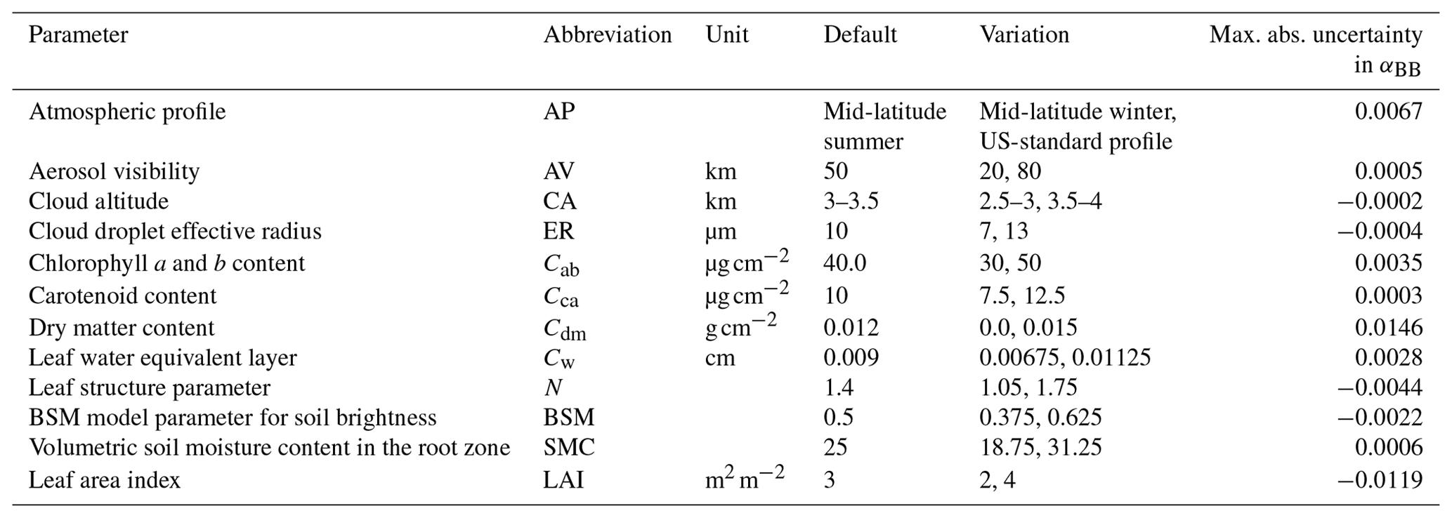
Within a homogeneous vegetation layer, the radiative transfer can be approximated by the turbid medium approach (Jones and Vaughan, 2010). The attenuation of direct radiance I0(λ) at the penetration depth z can be expressed by Eq. (7). Among other factors, the vegetation extinction coefficient kext(θ,λ) depends on the stand structure and canopy architecture, wavelength, direct and diffuse fractions of incident radiation, and incident angle θ (Bréda, 2003). It is therefore not straightforward to determine analytical expressions for kext(θ,λ) (Bréda, 2003; Jones and Vaughan, 2010). First-order approximations are provided, which do neglect the wavelength dependence of kext(θ,λ). It is also assumed that the solar zenith angle θ0 is equal to the incident angle θ. However, state-of-the-art vegetation radiative transfer (RT) models such as SCOPE2.0 account for wavelength-dependent effects by using numerical procedures (Yang et al., 2021). In the literature, various values of kext(θ) exist, ranging from fixed values (Pierce and Running, 1988; Wan et al., 2021) through empirical tabulated values (Bréda, 2003) to trigonometric functions that account for the dependence on the incident angle of radiation (Jones and Vaughan, 2010). Figure D1 shows kext(θ) as a function of θ for the spherical, erectophile, and planophile LADs. The planophile leaf angle distribution (LAD) is approximated with a value of kext(θ)=1. The spherical and erectophile LADs are described by the trigonometric functions given in Table D1. For θ<52°, kext(θ) of the spherical LAD exceeds kext(θ) of the erectophile LAD. The erectophile LAD is characterized by a steeper slope and, therefore, kext(θ) of the erectophile LAD is more sensitive to changes in θ. For θ>52°, kext(θ) of the erectophile LAD exceeds that of the spherical LAD, resulting in a larger kext(θ) with increasing θ. Note that extinction includes the processes of scattering and absorption, which means that an increase in kext(θ) means an increase in absorption in the canopy, but can also be caused by an increase in scattering.
The estimated values of kext(θ) are used to estimate the extinction of direct radiance in dependence of the LAI. Figure D2 shows that, for the Sun near the zenith (θ=25°), the slope is steepest for the planophile LAD, followed by the spherical and erectophile LADs. The incident direct radiation is reduced to 50 % (), when LAIs of 0.7, 2.3, and 1.26 for the planophile, spherical, and erectophile LADs are exceeded, respectively. For the Sun near the horizon (θ=70°), the slope is steepest for the erectophile LAD, followed by the spherical and planophile LADs. The ratio is reached at LAIs of 0.7, 0.4, and 0.5 for the planophile, erectophile, and LADs, respectively. As a result, for the default LAI of 3 and θ0=70°, the direct radiation cannot penetrate deeply into the canopy, while for the same LAI and θ0=25° the direct radiation can penetrate deepest into the canopy for the erectophile LAD, followed by the spherical and planophile LADs.
Table D1Vegetation extinction coefficient kext(θ) for the spherical, planophile, and erectophile leaf angle distributions, taken from Jones and Vaughan (2010).
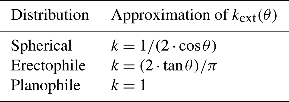
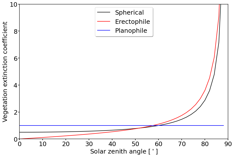
Figure D1Extinction coefficient as a function of incident angle θ for the spherical, erectophile, and planophile leaf angle distributions.
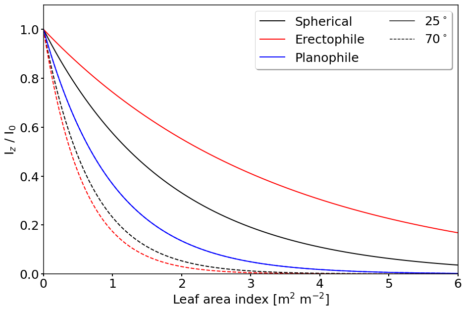
libRadtran and SCOPE2.0 are publicly available. Additional code for generating input files, reshaping the data, and data visualization is available upon request. Simulated spectra of irradiance and vegetation albedo are available via NetCDF files. The data are available on the Zenodo platform via https://doi.org/10.5281/zenodo.15275610 (Wolf et al., 2025).
The supplement related to this article is available online at https://doi.org/10.5194/bg-22-2909-2025-supplement.
KW designed and implemented the model coupling, performed the simulations, and drafted the manuscript. EJ, AE, MS, and MW contributed (equally) to the preparation of the manuscript. AH, HF, and AW helped with the model set-up and the revision of the manuscript.
The contact author has declared that none of the authors has any competing interests.
Publisher’s note: Copernicus Publications remains neutral with regard to jurisdictional claims made in the text, published maps, institutional affiliations, or any other geographical representation in this paper. While Copernicus Publications makes every effort to include appropriate place names, the final responsibility lies with the authors.
We thank the German Centre for Integrative Biodiversity Research (iDiv) Halle-Jena-Leipzig, which is a research center of the Deutsche Forschungsgemeinschaft (DFG). We also thank the Saxon State Ministry for Science, Culture and Tourism (SMWK) for funding through grant 3-7304/44/4-2023/8846.
This research has been supported by the Freistaat Sachsen (grant no. 3-7304/44/4-2023/8846).
This paper was edited by Andreas Ibrom and reviewed by Alexander Norton and one anonymous referee.
Aebi, C., Gröbner, J., Kazadzis, S., Vuilleumier, L., Gkikas, A., and Kämpfer, N.: Estimation of cloud optical thickness, single scattering albedo and effective droplet radius using a shortwave radiative closure study in Payerne, Atmos. Meas. Tech., 13, 907–923, https://doi.org/10.5194/amt-13-907-2020, 2020. a
Anderson, G. P., Clough, S. A., Kneizys, F. X., Chetwynd, J. H., and Shettle, E. P.: AFGL atmospheric constituent profiles, Environ. Res. Pap, 954, 1–46, 1986. a, b, c, d
Ardaneh, K., Maignan, F., Luyssaert, S., Peylin, P., and Boucher, O.: Fast, and accurate radiative transfer for land surface models, Procedia. Comput. Sci., 255, 3–12, https://doi.org/10.1016/j.procs.2025.02.255, 2025. a
Asner, G. P.: Biophysical and Biochemical Sources of Variability in Canopy Reflectance, Remote Sens. Environ., 64, 234–253, https://doi.org/10.1016/S0034-4257(98)00014-5, 1998. a, b, c, d
Atzberger, C.: Object-based retrieval of biophysical canopy variables using artificial neural nets and radiative transfer models, Remote Sens. Environ, 93, 53–67, https://doi.org/10.1016/j.rse.2004.06.016, 2004. a
Baldocchi, D. D., Wilson, K. B., and Gu, L.: How the environment, canopy structure and canopy physiological functioning influence carbon, water and energy fluxes of a temperate broad-leaved deciduous forest – an assessment with the biophysical model CANOAK, Tree Physiol., 22, 1065–1077, https://doi.org/10.1093/treephys/22.15-16.1065, 2002. a, b
Berk, A., Conforti, P., Kennett, R., Perkins, T., Hawes, F., and van den Bosch, J.: MODTRAN® 6: A major upgrade of the MODTRAN® radiative transfer code, in: 2014 6th workshop on hyperspectral image and signal processing: Evolution in remote sensing (WHISPERS), Lausanne, Switzerland, 24–27 June 2014, 1–4, https://doi.org/10.1109/WHISPERS.2014.8077573, 2014. a
Betts, R. A.: Offset of the potential carbon sink from boreal forestation by decreases in surface albedo, Nature, 408, 187–190, https://doi.org/10.1038/35041545, 2000. a
Bohren, C. F.: Multiple scattering of light and some of its observable consequences, Am. J. Phys, 55, 524–533, 1987. a, b
Boren, E. J., Boschetti, L., and Johnson, D. M.: Characterizing the variability of the structure parameter in the PROSPECT leaf optical properties model, Remote Sens., 11, 1236, https://doi.org/10.3390/rs11101236, 2019. a
Bosman, P. J. M., van Heerwaarden, C. C., and Teuling, A. J.: Sensible heating as a potential mechanism for enhanced cloud formation over temperate forest, Q. J. Roy. Meteor. Soc., 145, 450–468, https://doi.org/10.1002/qj.3441, 2019. a
Bounoua, L., DeFries, R., Collatz, G. J., Sellers, P., and Khan, H.: Effects of land cover conversion on surface climate, Clim. Change, 52, 29–64, https://doi.org/10.1023/A:1013051420309, 2002. a
Bowker, D. E.: Spectral reflectances of natural targets for use in remote sensing studies, vol. 1139, NASA, https://ntrs.nasa.gov/citations/19850022138 (last access: 19 June 2025), 1985. a
Bréda, N. J. J.: Ground‐based measurements of leaf area index: a review of methods, instruments and current controversies, J. Exp. Bot., 54, 2403–2417, https://doi.org/10.1093/jxb/erg263, 2003. a, b, c, d
Brodersen, C. R. and Vogelmann, T. C.: Do epidermal lens cells facilitate the absorptance of diffuse light?, Am. J. Bot., 94, 1061–1066, https://doi.org/10.3732/ajb.94.7.1061, 2007. a, b
Buras, R., Dowling, T., and Emde, C.: New secondary-scattering correction in DISORT with increased efficiency for forward scattering, J. Quant. Spectrosc. Ra., 112, 2028–2034, https://doi.org/10.1016/j.jqsrt.2011.03.019, 2011. a
Cerasoli, S., Yin, J., and Porporato, A.: Cloud cooling effects of afforestation and reforestation at midlatitudes, P. Natl. Acad. Sci. USA, 118, e2026241118, https://doi.org/10.1073/pnas.2026241118, 2021. a
Chen, Q., Baldocchi, D., Gong, P., and Dawson, T.: Modeling radiation and photosynthesis of a heterogeneous savanna woodland landscape with a hierarchy of model complexities, Agr. Forest Meteorol., 148, 1005–1020, https://doi.org/10.1016/j.agrformet.2008.01.020, 2008. a
Cheng, S. J., Steiner, A. L., Hollinger, D. Y., Bohrer, G., and Nadelhoffer, K. J.: Using satellite-derived optical thickness to assess the influence of clouds on terrestrial carbon uptake, J. Geophys. Res.-Biogeo., 121, 1747–1761, https://doi.org/10.1002/2016JG003365, 2016. a
Coddington, O. M., Richard, E. C., Harber, D., Pilewskie, P., Woods, T. N., Chance, K., Liu, X., and Sun, K.: The TSIS-1 Hybrid Solar Reference Spectrum, Geophys. Res. Let., 48, e2020GL091709, https://doi.org/10.1029/2020GL091709, 2021. a
Damm, A., Guanter, L., Verhoef, W., Schläpfer, D., Garbari, S., and Schaepman, M. E.: Impact of varying irradiance on vegetation indices and chlorophyll fluorescence derived from spectroscopy data, Remote Sens. Environ., 156, 202–215, https://doi.org/10.1016/j.rse.2014.09.031, 2015. a
Davidson, A. and Wang, S.: The effects of sampling resolution on the surface albedos of dominant land cover types in the North American boreal region, Remote Sens. Environ., 93, 211–224, https://doi.org/10.1016/j.rse.2004.07.005, 2004. a, b
Davidson, A. and Wang, S.: Spatiotemporal variations in land surface albedo across Canada from MODIS observations, C. J. Remote Sens., 31, 377–390, https://doi.org/10.5589/m05-021, 2005. a, b
Deering, D. W. and Eck, T. F.: Atmospheric optical depth effects on angular anisotropy of plant canopy reflectance, Int. J. Remote Sens., 8, 893–916, 1987. a
Dye, D. G.: Spectral composition and quanta-to-energy ratio of diffuse photosynthetically active radiation under diverse cloud conditions, J. Geophys. Res.-Atmos., 109, D10203, https://doi.org/10.1029/2003JD004251, 2004. a
Eastman, R., G., W. S., and Hahn, C. J.: Variations in cloud cover and cloud types over the ocean from surface observations, 1954–2008, J. Climate, 24, 5914–5934, https://doi.org/10.1175/2011JCLI3972.1, 2011. a
ECMWF: IFS documentation CY47R3 – Part IV physical processes, 4, ECMWF, https://doi.org/10.21957/eyrpir4vj, 2021. a, b, c
Emde, C., Buras-Schnell, R., Kylling, A., Mayer, B., Gasteiger, J., Hamann, U., Kylling, J., Richter, B., Pause, C., Dowling, T., and Bugliaro, L.: The libRadtran software package for radiative transfer calculations (version 2.0.1), Geosci. Model Dev., 9, 1647–1672, https://doi.org/10.5194/gmd-9-1647-2016, 2016. a, b, c
Eugster, W., Rouse, W. R., Pielke Sr, R. A., Mcfadden, J. P., Baldocchi, D. D., Kittel, T. G. F., Chapin III, F. S., Liston, G. E., Vidale, P. L., Vaganov, E., and Chambers, S.: Land–atmosphere energy exchange in Arctic tundra and boreal forest: available data and feedbacks to climate, Global Change Biol., 6, 84–115, https://doi.org/10.1046/j.1365-2486.2000.06015.x, 2000. a, b
Freedman, J. M., Fitzjarrald, D. R., Moore, K. E., and Sakai, R. K.: Boundary layer clouds and vegetation–atmosphere feedbacks, J. Climate, 14, 180–197, https://doi.org/10.1175/1520-0442(2001)013<0180:BLCAVA>2.0.CO;2, 2001. a, b, c, d, e, f, g
Frisch, S., Shupe, M., Djalalova, I., Feingold, G., and Poellot, M.: The retrieval of stratus cloud droplet effective radius with cloud radars, J. Atmos. Ocean. Tech., 19, 835–842, https://doi.org/10.1175/1520-0426(2002)019<0835:TROSCD>2.0.CO;2, 2002. a
Gasteiger, J., Emde, C., Mayer, B., Buras, R., Buehler, S., and Lemke, O.: Representative wavelengths absorption parameterization applied to satellite channels and spectral bands, J. Quant. Spectrosc. Ra., 148, 99–115, https://doi.org/10.1016/j.jqsrt.2014.06.024, 2014. a
Goel, N. S.: Models of vegetation canopy reflectance and their use in estimation of biophysical parameters from reflectance data, Remote Sens. Rev., 4, 1–212, https://doi.org/10.1080/02757258809532105, 1988. a
Goel, N. S. and Strebel, D. E.: Simple beta distribution representation of leaf orientation in vegetation canopies, Agro. J., 76, 800–802, https://doi.org/10.2134/agronj1984.00021962007600050021x, 1984. a
Gorton, H. L., Brodersen, C. R., Williams, W. E., and Vogelmann, T. C.: Measurement of the optical properties of leaves under diffuse light, Photochem. Photobiol., 86, 1076–1083, https://doi.org/10.1111/j.1751-1097.2010.00761.x, 2010. a, b
Grant, L.: Diffuse and specular characteristics of leaf reflectance, Remote Sens. Environ., 22, 309–322, https://doi.org/10.1016/0034-4257(87)90064-2, 1987. a
Grenfell, T. C. and Perovich, D. K.: Incident spectral irradiance in the Arctic Basin during the summer and fall, J. Geophys. Res.-Atmos., 113, D12117, https://doi.org/10.1029/2007JD009418, 2008. a
Gueymard, C. A.: Cloud and albedo enhancement impacts on solar irradiance using high-frequency measurements from thermopile and photodiode radiometers. Part 1: Impacts on global horizontal irradiance, Sol. Energy, 153, 755–765, https://doi.org/10.1016/j.solener.2017.05.004, 2017. a, b, c, d
Gueymard, C. A. and Ruiz-Arias, J. A.: Extensive worldwide validation and climate sensitivity analysis of direct irradiance predictions from 1-min global irradiance, Sol. Energy, 128, 1–30, https://doi.org/10.1016/j.solener.2015.10.010, 2016. a
Hay, J. E.: A revised method for determining the direct and diffuse components of the total short‐wave radiation, Atmosphere, 14, 278–287, https://doi.org/10.1080/00046973.1976.9648423, 1976. a
Henniger, H., Bohn, F. J., Schmidt, K., and Huth, A.: A new approach combining a multilayer radiative transfer model with an individual-based forest model: Application to boreal forests in Finland, Remote Sens., 15, 3078, https://doi.org/10.3390/rs15123078, 2023. a
Houborg, R. and Boegh, E.: Mapping leaf chlorophyll and leaf area index using inverse and forward canopy reflectance modeling and SPOT reflectance data, Remote Sens. Environ., 112, 186–202, https://doi.org/10.1016/j.rse.2007.04.012, 2008. a
Hovi, A., Lukes̆, P., and Rautiainen, M.: Seasonality of albedo and FAPAR in a boreal forest, Agr. Forest Meteorol., 247, 331–342, https://doi.org/10.1016/j.agrformet.2017.08.021, 2017. a
Irvine, W. M. and Pollack, J. B.: Infrared optical properties of water and ice spheres, Icarus, 8, 324–360, https://doi.org/10.1016/0019-1035(68)90083-3, 1968. a
Jones, H. G. and Vaughan, R. A.: Remote sensing of vegetation: principles, techniques, and applications, Oxford University Press, USA, ISBN 978-0199207794, 2010. a, b, c, d, e, f, g, h, i, j, k, l, m, n
Kanniah, K. D., Beringer, J., North, P., and Hutley, L.: Control of atmospheric particles on diffuse radiation and terrestrial plant productivity: A review, Prog. Phys. Geogr., 36, 209–237, https://doi.org/10.1177/0309133311434244, 2012. a, b, c, d, e
Kierkus, W. T. and Colborne, W. G.: Diffuse solar radiation – Daily and monthly values as affected by snow cover, Sol. Energy, 42, 143–147, https://doi.org/10.1016/0038-092X(89)90141-2, 1989. a
King, M. D.: Determination of the scaled optical thickness of clouds from reflected solar radiation measurements, J. Atmos. Sci., 44, 1734–1751, https://doi.org/10.1175/1520-0469(1987)044<1734:DOTSOT>2.0.CO;2, 1987. a
Kokhanovsky, A. A.: Light scattering reviews 4: single light scattering and radiative transfer, Springer Science & Business Media, ISBN 978-3540742753, 2009. a
Kötz, B., Schaepman, M., Morsdorf, F., Bowyer, P., Itten, K., and Allgöwer, B.: Radiative transfer modeling within a heterogeneous canopy for estimation of forest fire fuel properties, Remote Sens. Environ., 92, 332–344, https://doi.org/10.1016/j.rse.2004.05.015, 2004. a
Kubelka, P.: Ein Beitrag zur Optik der Farbanstriche, Z. Tech. Phys., 12, 593–601, 1931. a, b
Li, F., Hao, D., Zhu, Q., Yuan, K., Braghiere, R. K., He, L., Luo, X., Wei, S., Riley, W. J., Zeng, Y., and Chen, M.: Vegetation clumping modulates global photosynthesis through adjusting canopy light environment, Global Change Biol., 29, 731–746, https://doi.org/10.1111/gcb.16503, 2023. a, b
Liang, X.-Z., Xu, M., Gao, W., Kunkel, K., Slusser, J., Dai, Y., Min, Q., Houser, P. R., Rodell, M., Schaaf, C. B., and Gao, F.: Development of land surface albedo parameterization based on Moderate Resolution Imaging Spectroradiometer (MODIS) data, J. Geophys. Res.-Atmos., 110, D11107, https://doi.org/10.1029/2004JD005579, 2005. a
Liu, C. H., Chen, A. J., and Liu, G. R.: Variability of the bare soil albedo due to different solar zenith angles and atmospheric haziness, Int. J. Remote Sens., 15, 2531–2542, 1994. a
Loveland, T. R. and Belward, A. S.: The IGBP-DIS global 1km land cover data set, DISCover: First results, Int. J. Remote Sens., 18, 3289–3295, https://doi.org/10.1080/014311697217099, 1997. a, b
Lucht, W., Schaaf, C., and Strahler, A.: An algorithm for the retrieval of albedo from space using semiempirical BRDF models, IEEE T. Geosci. Remote, 38, 977–998, https://doi.org/10.1109/36.841980, 2000. a
Lyapustin, A. I. and Privette, J. L.: A new method of retrieving surface bidirectional reflectance from ground measurements: Atmospheric sensitivity study, J. Geophys. Res.-Atmos., 104, 6257–6268, https://doi.org/10.1029/1998JD200123, 1999. a
Majasalmi, T. and Rautiainen, M.: The impact of tree canopy structure on understory variation in a boreal forest, Forest Ecol. Manage., 466, 118 100, https://doi.org/10.1016/j.foreco.2020.118100, 2020. a
Martonchik, J. V., Bruegge, C. J., and Strahler, A. H.: A review of reflectance nomenclature used in remote sensing, Remote Sens. Rev., 19, 9–20, https://doi.org/10.1080/02757250009532407, 2009. a
Mie, G.: Beiträge zur Optik trüber Medien, speziell kolloidaler Metallösungen, Ann. Phys., 330, 377–445, https://doi.org/10.1002/andp.19083300302, 1908. a, b
Min, Q.: Impacts of aerosols and clouds on forest-atmosphere carbon exchange, J. Geophys. Res.-Atmos., 110, D06203, https://doi.org/10.1029/2004JD004858, 2005. a
Min, Q. and Wang, S.: Clouds modulate terrestrial carbon uptake in a midlatitude hardwood forest, Geophys. Res. Lett., 35, L02406, https://doi.org/10.1029/2007GL032398, 2008. a, b, c
Moene, A. F. and Van Dam, J. C.: Transport in the atmosphere-vegetation-soil continuum, Cambridge University Press, ISBN 978-0521195683, 2014. a
Monsi, M.: Uber den Lichtfaktor in den Pflanzengesellschaften und seine Bedeutung fur die Stoffproduktion, Jap. J. Bot., 14, 22–52, 1953. a
Myhre, G., Kvalevåg, M. M., and Schaaf, C. B.: Radiative forcing due to anthropogenic vegetation change based on MODIS surface albedo data, Geophys. Res. Lett., 32, L21410, https://doi.org/10.1029/2005GL024004, 2005. a
Nakajima, T., King, M. D., Spinhirne, J. D., and Radke, L. F.: Determination of the optical thickness and effective particle radius of clouds from reflected solar radiation measurements. Part II: marine stratocumulus observations, J. Atmos. Sci., 48, 728–751, https://doi.org/10.1175/1520-0469(1991)048<0728:DOTOTA>2.0.CO;2, 1991. a
Nemani, R. R., Keeling, C. D., Hashimoto, H., Jolly, W. M., Piper, S. C., Tucker, C. J., Myneni, R. B., and Running, S. W.: Climate-driven increases in global terrestrial net primary production from 1982 to 1999, Science, 300, 1560–1563, https://doi.org/10.1126/science.1082750, 2003. a
Ni, W. and Woodcock, C. E.: Effect of canopy structure and the presence of snow on the albedo of boreal conifer forests, J. Geophys. Res.-Atmos., 105, 11879–11888, https://doi.org/10.1029/1999JD901158, 2000. a
Ni-Meister, W., Yang, W., and Kiang, N. Y.: A clumped-foliage canopy radiative transfer model for a global dynamic terrestrial ecosystem model. I: Theory, Agr. Forest Meteorol., 150, 881–894, https://doi.org/10.1016/j.agrformet.2010.02.009, 2010. a
Ollinger, S. V.: Sources of variability in canopy reflectance and the convergent properties of plants, New Phytol., 189, 375–394, https://doi.org/10.1111/j.1469-8137.2010.03536.x, 2011. a, b
Parisi, A. V., Sabburg, J., Kimlin, M. G., and Downs, N.: Measured and modelled contributions to UV exposures by the albedo of surfaces in an urban environment, Theor. Appl. Climatol., 76, 181–188, https://doi.org/10.1007/s00704-003-0012-9, 2003. a
Pierce, L. L. and Running, S. W.: Rapid estimation of coniferous forest leaf area index using a portable integrating radiometer, Ecology, 69, 1762–1767, https://doi.org/10.2307/1941154, 1988. a
Pisek, J., Diaz-Pines, E., Matteucci, G., Noe, S., and Rebmann, C.: On the leaf inclination angle distribution as a plant trait for the most abundant broadleaf tree species in Europe, Agr. Forest Meteorol., 323, 109030, https://doi.org/10.1016/j.agrformet.2022.109030, 2022. a, b
Qin, H., Wang, C., Zhao, K., and Xi, X.: Estimation of the fraction of absorbed photosynthetically active radiation (fPAR) in maize canopies using LiDAR data and hyperspectral imagery, Plos One, 13, e0197510, https://doi.org/10.1371/journal.pone.0197510, 2018. a
Ranson, K. J., Biehl, L. L., and Bauer, M. E.: Variation in spectral response of soybeans with respect to illumination, view and canopy geometry, Int. J. Remote Sens., 6, 1827–1842, 1985. a
Roderick, M. L., Farquhar, G. D., Berry, S. L., and Noble, I. R.: On the direct effect of clouds and atmospheric particles on the productivity and structure of vegetation, Oecologia, 129, 21–30, 2001. a
Schaepman-Strub, G., Schaepman, M. E., Painter, T. H., Dangel, S., and Martonchik, J. V.: Reflectance quantities in optical remote sensing-definitions and case studies, Remote Sens. Environ., 103, 27–42, https://doi.org/10.1016/j.rse.2006.03.002, 2006. a, b, c
Shettle, E. P.: Models of aerosols, clouds and precipitation for atmo- spheric propagation studies, in: Atmospheric propagation in the uv, visible, ir and mm-region and related system aspects, no. 454 in AGARD Conference Proceedings, https://ui.adsabs.harvard.edu/abs/1990apuv.agar.....S/abstract (last access: 19 June 2025), 1989. a
Sinoquet, H., Le Roux, X., Adam, B., Ameglio, T., and Daudet, F. A.: RATP: a model for simulating the spatial distribution of radiation absorption, transpiration and photosynthesis within canopies: application to an isolated tree crown, Plant Cell. Environ., 24, 395–406, https://doi.org/10.1046/j.1365-3040.2001.00694.x, 2001. a
Stamnes, K., Tsay, S.-C., Wiscombe, W., and Jayaweera, K.: Numerically stable algorithm for discrete-ordinate-method radiative transfer in multiple scattering and emitting layered media, Appl. Opt., 27, 2502–2509, https://doi.org/10.1364/AO.27.002502, 1988. a
Stapf, J., Ehrlich, A., Jäkel, E., Lüpkes, C., and Wendisch, M.: Reassessment of shortwave surface cloud radiative forcing in the Arctic: consideration of surface-albedo–cloud interactions, Atmos. Chem. Phys., 20, 9895–9914, https://doi.org/10.5194/acp-20-9895-2020, 2020. a
Stenberg, P., Lukeš, P., Rautiainen, M., and Manninen, T.: A new approach for simulating forest albedo based on spectral invariants, Remote Sens. Environ., 137, 12–16, https://doi.org/10.1016/j.rse.2013.05.030, 2013. a
Stephens, G. L.: Remote sensing of the lower atmosphere, an introduction, Oxford University Press, New York, ISBN 978-0195081889, 1994. a
Stuckens, J., Somers, B., Delalieux, S., Verstraeten, W. W., and Coppin, P.: The impact of common assumptions on canopy radiative transfer simulations: A case study in Citrus orchards, J. Quant. Spectrosc. Ra., 110, 1–21, https://doi.org/10.1016/j.jqsrt.2008.09.001, 2009. a, b
Tselioudis, G., Rossow, W. B., and Rind, D.: Global patterns of cloud optical thickness variation with temperature, J. Climate, 5, 1484–1495, https://doi.org/10.1175/1520-0442(1992)005<1484:GPOCOT>2.0.CO;2, 1992. a
Verhoef, W.: Light scattering by leaf layers with application to canopy reflectance modeling: The SAIL model, Remote Sens. Environ., 16, 125–141, https://doi.org/10.1016/0034-4257(84)90057-9, 1984. a
Verhoef, W.: Theory of radiative transfer models applied in optical remote sensing of vegetation canopies, PhD thesis, Wageningen University and Research, https://edepot.wur.nl/210943 (last access: 19 June 2025), 1998. a
Verhoef, W., van der Tol, C., and Middleton, E. M.: Hyperspectral radiative transfer modeling to explore the combined retrieval of biophysical parameters and canopy fluorescence from FLEX – Sentinel-3 tandem mission multi-sensor data, Remote Sens. Environ., 204, 942–963, https://doi.org/10.1016/j.rse.2017.08.006, 2018. a
Verrelst, J., Rivera, J. P., van der Tol, C., Magnani, F., Mohammed, G., and Moreno, J.: Global sensitivity analysis of the SCOPE model: What drives simulated canopy-leaving sun-induced fluorescence?, Remote Sens. Environ., 166, 8–21, https://doi.org/10.1016/j.rse.2015.06.002, 2015. a, b
Vicari, M. B., Pisek, J., and Disney, M.: New estimates of leaf angle distribution from terrestrial LiDAR: Comparison with measured and modelled estimates from nine broadleaf tree species, Agr. Forest Meteorol., 264, 322–333, https://doi.org/10.1016/j.agrformet.2018.10.021, 2019. a, b, c
Vilfan, N., van der Tol, C., Muller, O., Rascher, U., and Verhoef, W.: Fluspect-B: A model for leaf fluorescence, reflectance and transmittance spectra, Remote Sens. Environ., 186, 596–615, https://doi.org/10.1016/j.rse.2016.09.017, 2016. a
Vilfan, N., Van der Tol, C., Yang, P., Wyber, R., Malenovský, Z., Robinson, S. A., and Verhoef, W.: Extending Fluspect to simulate xanthophyll driven leaf reflectance dynamics, Remote Sens. Environ., 211, 345–356, https://doi.org/10.1016/j.rse.2018.04.012, 2018. a
Wan, L., Zhu, J., Du, X., Zhang, J., Han, X., Zhou, W., Li, X., Liu, J., Liang, F., He, Y., and Cen, H.: A model for phenotyping crop fractional vegetation cover using imagery from unmanned aerial vehicles, J. Exp. Bot., 72, 4691–4707, https://doi.org/10.1093/jxb/erab194, 2021. a
Warren, S. G.: Optical properties of snow, Rev. Geophys., 20, 67–89, https://doi.org/10.1029/RG020i001p00067, 1982. a, b, c
Watson, D. J.: Comparative physiological studies on the growth of field crops: I. Variation in net assimilation rate and leaf area between species and varieties, and within and between years, Ann. Bot., 11, 41–76, 1947. a, b
Weihs, P., Lenoble, J., Blumthaler, M., Martin, T., Seckmeyer, G., Philipona, R., De la Casiniere, A., Sergent, C., Gröbner, J., Cabot, T., Masserot, D., Pichler, T., Pougatch, E., Rengarajan, G., Schmucki, D., and Simic, S.: Modeling the effect of an inhomogeneous surface albedo on incident UV radiation in mountainous terrain: Determination of an effective surface albedo, Geophys. Res. Lett., 28, 3111–3114, https://doi.org/10.1029/2001GL012986, 2001. a
Wendisch, M. and Yang, P.: Theory of atmospheric radiative transfer: A comprehensive introduction, Wiley, ISBN 9783527408368, 2012. a
Wendisch, M., Pilewskie, P., Jäkel, E., Schmidt, S., Pommier, J., Howard, S., Jonsson, H. H., Guan, H., Schröder, M., and Mayer, B.: Airborne measurements of areal spectral surface albedo over different sea and land surfaces, J. Geophys. Res. Atmos., 109, D08203, https://doi.org/10.1029/2003JD004392, 2004. a, b
Wiscombe, W. J. and Warren, S. G.: A model for the spectral albedo of snow. I: pure snow, J. Atmos. Sci., 37, 2712–2733, https://doi.org/10.1175/1520-0469(1980)037<2712:AMFTSA>2.0.CO;2, 1980. a, b, c, d
Yan, H., Wang, S., Dai, J., Wang, J., Chen, J., and Shugart, H. H.: Forest greening increases land surface albedo during the main growing period between 2002 and 2019 in China, J. Geophys. Res.-Atmos., 126, e2020JD033582, https://doi.org/10.1029/2020JD033582, 2021. a
Wolf, K., Jäkel, E., Ehrlich, A., Schäfer, M., Feilhauer, H., Huth, A., and Wendisch, M.: Simulated spectral irradiances, radiances, and vegetation albedo obtained from coupling libRadtran and SCOPE2.0, Zenodo [data set], https://doi.org/10.5281/zenodo.15275610, 2025. a
Yang, P., Verhoef, W., and van der Tol, C.: The mSCOPE model: A simple adaptation to the SCOPE model to describe reflectance, fluorescence and photosynthesis of vertically heterogeneous canopies, Remote Sens. Environ., 201, 1–11, https://doi.org/10.1016/j.rse.2017.08.029, 2017. a
Yang, P., van der Tol, C., Yin, T., and Verhoef, W.: The SPART model: A soil-plant-atmosphere radiative transfer model for satellite measurements in the solar spectrum, Remote Sens. Environ., 247, 111870, https://doi.org/10.1016/j.rse.2020.111870, 2020. a, b, c, d
Yang, P., Prikaziuk, E., Verhoef, W., and van der Tol, C.: SCOPE 2.0: a model to simulate vegetated land surface fluxes and satellite signals, Geosci. Model Dev., 14, 4697–4712, https://doi.org/10.5194/gmd-14-4697-2021, 2021. a, b, c, d, e, f
Yang, X., Li, R., Jablonski, A., Stovall, A., Kim, J., Yi, K., Ma, Y., Beverly, D., Phillips, R., Novick, K., Xu, X., and Lerdau, M.: Leaf angle as a leaf and canopy trait: Rejuvenating its role in ecology with new technology, Ecol. Lett., 26, 1005–1020, https://doi.org/10.1111/ele.14215, 2023. a, b
Zhang, Y. and Klein, S. A.: Factors controlling the vertical extent of fair-weather shallow cumulus clouds over land: Investigation of diurnal-cycle observations collected at the ARM Southern Great Plains site, J. Atmos. Sci., 70, 1297–1315, https://doi.org/10.1175/JAS-D-12-0131.1, 2013. a
Zheng, L., Zhao, G., Dong, J., Ge, Q., Tao, J., Zhang, X., Qi, Y., Doughty, R. B., and Xiao, X.: Spatial, temporal, and spectral variations in albedo due to vegetation changes in China’s grasslands, ISPRS J. Photogramm. Remote Sens., 152, 1–12, https://doi.org/10.1016/j.isprsjprs.2019.03.020, 2019. a
- Abstract
- Introduction
- Terminology, radiative transfer simulations, and iterative coupling
- Results and discussion
- Summary and conclusions
- Appendix A: Sensitivity of broadband solar albedo for the full range of cloud optical thickness
- Appendix B: Influence of clouds on downward irradiance
- Appendix C: Uncertainty estimates due to selection of default parameters
- Appendix D: Approximate direct beam extinction in vegetation
- Code and data availability
- Author contributions
- Competing interests
- Disclaimer
- Acknowledgements
- Financial support
- Review statement
- References
- Supplement