Three-compartment, two-parameter concentration-driven model for uptake of excess atmospheric CO₂ by the global ocean

This paper develops, applies, and examines a transparent three-compartment model for the amounts of CO₂ (dissolved inorganic carbon, DIC) in the mixed-layer and deep oceans over the Anthropocene, driven by the observed amount of atmospheric CO₂. The model has two independent parameters, a piston velocity v_p characterizing the rate of water exchange between the mixed-layer ocean (ML) and the deep ocean (DO), and an atmosphere–ocean deposition velocity for low- to intermediate-solubility gases k_am. The net uptake of CO₂ into the ocean is only weakly dependent on k_am, so the net uptake rate depends almost solely on v_p. This piston velocity is determined from the measured rate of uptake of heat by the global ocean from the 1960s to the present as 7.5 ± 2.2 m yr⁻¹, 1σ. The resultant modeled net uptake flux of anthropogenic atmospheric CO₂ by the global ocean in the year 2022 is 2.84 ± 0.6 Pg yr⁻¹, and the corresponding net transfer coefficient – the net anthropogenic uptake flux divided by the stock of excess atmospheric CO₂ – is 0.010 ± 0.002 yr⁻¹. This net transfer coefficient appears to decrease slightly (∼ 17 %) over the Anthropocene; this decrease is attributed to the decrease in the equilibrium solubility of CO₂ (as dissolved inorganic carbon) in seawater due to the uptake of additional CO₂ over this period and slightly increasing return flux from the DO to the ML. Modeled DIC in the global ocean and net atmosphere–ocean fluxes compare well with observations and with current carbon cycle models (both concentration driven and emissions driven). Uptake of anthropogenic carbon by the terrestrial biosphere is calculated as the difference between emissions and the sum of increases in atmospheric and ocean stocks. The model, used to calculate radiocarbon over the industrial era (over the period during which radiocarbon was influenced by emissions of ¹⁴C-free CO₂, mainly from fossil fuel combustion) and the period dominated by ¹⁴C emissions from atmospheric weapons testing, compares well with available measurements of ocean radiocarbon and with other models. A variant of the model with only two compartments and a single parameter, v_p, treating the atmosphere and the mixed-layer ocean as a single compartment in equilibrium, performs essentially as well as the three-compartment, two-parameter model. Although the concentration-driven model developed here cannot be used prognostically (to assess model skill in replicating atmospheric CO₂ over the industrial period or to examine response to changes in emissions), the model is useful diagnostically to examine the disposition of excess carbon into pertinent global compartments as a function of time over the Anthropocene. More importantly, the model and the parameters developed here can be used with confidence to represent ocean uptake of excess CO₂ in emissions-driven models.

1 Introduction

About 250 years ago, humankind initiated what has been characterized (Revelle and Suess, 1957; Ramanathan, 1988) as an inadvertent global geophysical experiment by emitting carbon dioxide (CO₂) into the atmosphere, in conjunction with the combustion of fossil fuels, other industrial activities, and changes in land use, thereby changing Earth's climate. Anthropogenic CO₂, the amount in excess of preindustrial (PI) levels, affects Earth's radiation budget, with present radiative forcing relative to preindustrial levels of about 2.2 W m⁻² (Forster et al., 2021), and acidifies the ocean, with the present decrease in the pH of the surface ocean relative to preindustrial levels being about 0.11 (Jiang et al., 2019).

Much attention has been paid to the uptake of excess CO₂ by the global ocean because of the importance of this uptake as a sink for anthropogenic CO₂. The processes governing this uptake are relatively straightforward and rather well understood: dissolution of CO₂ at the air–sea interface (including its dependence on the abundance of atmospheric CO₂) and transport and mixing of dissolved inorganic carbon as a conservative tracer in the global ocean. Exchange processes between the atmosphere and the mixed-layer ocean (ML) (upper ocean, a depth of roughly 100 m) and within the ML are rapid but, because of the small volume of the ML, do not contribute greatly to uptake of CO₂ by the global ocean. The majority of this uptake is into the deep ocean (DO), with the overall rate of uptake controlled mainly by the rates of transport and mixing between the ML and the DO, which take place on decadal timescales (Broecker and Peng, 1974; Oeschger et al., 1975; Sarmiento et al., 1992; Graven et al., 2012). A recent review (Gruber et al., 2023) found that the current net rate of uptake of CO₂ by the global ocean is 2.7 ± 0.3 Pg(C) yr⁻¹ (1 Pg = 10¹⁵ g). This net uptake constitutes about 24 % of total anthropogenic emissions from fossil fuel combustion and net emissions from land-use change, about 11 Pg yr⁻¹.

Historically, studies examining the budget of excess CO₂ in the atmosphere and carbon in other reservoirs were based on so-called compartment models, in which the global and annual amounts of excess atmospheric CO₂ and carbon derived from atmospheric CO₂ were represented in a small number of compartments, typically up to about half a dozen. The strengths of such models were that the number of parameters characterizing the transport of carbon between the reservoirs was small (also up to about half a dozen), that such transfer coefficients could be constrained by observations, and that the propagated uncertainties associated with the transfer coefficients could be readily examined. In other words, the models were transparent. In recent decades, especially with the increase in understanding of the processes controlling the transfer of carbon among the reservoirs (mainly air–sea exchange, ocean transport, and terrestrial photosynthesis and respiration), together with the increase in numerical modeling capability afforded by modern computers, the tendency has been toward detailed modeling of the carbon cycle by so-called carbon cycle models with increasingly high spatial (both horizontal and vertical) and temporal resolutions, representing the rates of processes in tens of thousands of compartments by dozens to hundreds of parameters that in turn depend on numerous situational variables such as temperature and wind speed and, for the terrestrial biosphere (TB), water availability, insolation, and other controlling variables for numerous vegetation types. While this approach has led to a much more detailed representation of the exchange of carbon between the atmosphere, the ocean, and the TB, it has resulted in attendant loss of the transparency of the models.

The present study returns to the earlier approach of representing global stocks of anthropogenic carbon in a few global compartments. The present paper is the first in a series that uses models with a small number of global compartments to represent the evolution of anthropogenic carbon in the atmosphere and in closely coupled compartments of the biogeosphere. In this paper a simple concentration-driven model for net uptake of atmospheric CO₂ by the global ocean is developed, and results are presented and compared to observations and other models; the model is driven by the measured stock S_a of CO₂ in the atmosphere (at preindustrial (PI) time and as a function of time over the Anthropocene, taken here as commencing in the year 1750). Uptake of anthropogenic CO₂ by the ML and the DO is actively modeled using transfer coefficients developed here. Uptake into the TB is not actively modeled but is regarded as being equal to the difference between total emissions and the uptake and growth in the atmosphere and the ocean. Anthropogenic emissions, the stock in the TB, and the net flux between the atmosphere and the TB are presented only for reference to the total budget. A central objective of the present study is that the parameters of the model be traceable to observations. Although there are other recent studies that develop and use models with a small number of compartments (e.g., Glotter et al., 2014; McKinley et al., 2020; Martínez Montero et al., 2022), key parameters in those studies are simply specified as “reasonable” or as “adjusted to match the dynamics of more complex carbon cycle models” and are thus not traceable to observations.

Because the model presented here is concentration driven, it is diagnostic, not prognostic. That is, the results show the disposition of anthropogenically emitted carbon in the atmosphere, the ML, and the DO, and, by difference, the TB, as a function of time over the Anthropocene. Importantly, the concentration-driven model cannot be used to calculate the stocks in the several compartments for historical emissions or for prospective future emissions. Nonetheless, to the extent that this concentration-driven model accurately yields this disposition, the representation of the processes in the model can then be incorporated with confidence into emissions-driven models, as will be done in subsequent papers.

In this paper, S_i denotes the stocks of CO₂ or dissolved inorganic carbon (DIC) as the mass of carbon, C (not CO₂), in petagrams (10¹⁵ g, Pg), in a given compartment i denoted by subscripts a, m, d, and t for the atmosphere, mixed-layer ocean (ML), deep ocean (DO), and terrestrial biosphere (TB), respectively. $S_i^{\mathrm{ant}}$ denotes anthropogenic stock (excess above preindustrial levels) in compartment i. F_ij denotes the gross flux from compartment i to compartment j; $F_{ij}^{\mathrm{net}}$ denotes the net flux from compartment i to j and is equal to F_ij−F_ji. Transfer coefficients k_ij (yr⁻¹) denote flux F_ij per stock of the leaving compartment S_i; similarly, $k_{ij}^{\mathrm{net}}$ denotes the net flux per anthropogenic stock in the leaving compartment, and $k_i^{\mathrm{net},\mathrm{ant}}$ denotes the net flux per anthropogenic stock in the leaving compartment. Q_ant (in petagrams per year) denotes the anthropogenic emission rate, $Q_{\mathrm{ant}}^{\mathrm{ff}}$ denotes the sum of emissions from fossil fuel combustion and cement manufacturing, and $Q_{\mathrm{ant}}^{\mathrm{lu}}$ denotes land-use change. Subscripts or superscripts pi, pd, and ant denote the preindustrial, present-day, and anthropogenic components of a stock or flux, respectively.

This paper is organized as follows. Section 2 presents an overview of the compartments comprising the carbon system. Section 3 develops the transfer coefficients describing the rates of transfer between the several compartments used as input to the model. Section 4 presents the preindustrial stocks in the several compartments used to initiate the model and the time-dependent stock of CO₂ in the atmosphere used to force the model calculations. It also presents historical emissions, which, although not directly used in the model calculation, are needed to calculate, by difference, the stock in the terrestrial biosphere and its rate of growth over the Anthropocene. Section 5 develops the model, presents results obtained in the calculations for normal CO₂ and for radiocarbon, and also develops and examines a variant of the model in which the stocks in the atmosphere and the ML are treated in equilibrium. Section 6 compares the results obtained in the model calculations with results from other model studies and with observations. Section 7 presents the discussion and conclusions. There are two appendices. Appendix A discusses the equilibrium solubility of CO₂ in seawater, specifically the dissolution reactions that form bicarbonate and carbonate ions. Appendix B presents the treatment of the rate of mass transfer of CO₂ between the atmosphere and the ocean, taking into account the solubility equilibria.

The paper makes extensive use of figures to present the results of the calculations, principally as time series, and to compare to other calculations and observations. The intent of this paper is to make the model, the reasoning that went into the development of the model, and the results as fully transparent as possible. All the data from the present model calculations are provided as supplement data in a single Excel workbook.

2 Overview

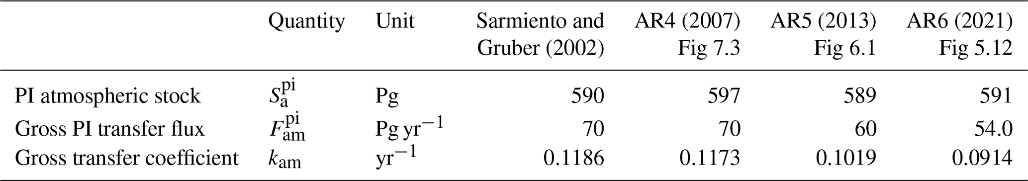
The framework of the global carbon budget developed here is given in Fig. 1. The template for this budget is Fig. 7.3 from the Fourth IPCC Assessment Report (AR4; Denman et al., 2007), which, in turn, is based on a figure initially given by Sarmiento and Gruber (2002); the values of anthropogenic stocks and fluxes have been updated to reflect the early 2020s time frame. Similar figures have been presented in the several recent IPCC assessment reports, namely the Fifth Assessment Report (AR5; Ciais et al., 2013, Fig. 6.1, Table 6.1) and the Sixth Assessment Report (AR6; Canadell et al., 2021, Fig. 5.12), with antecedents going back to at least AR1 (Watson et al., 1990, Fig. 1.1). This budget is based on observations: PI and present-day (PD) values and annual increment of the atmospheric CO₂ mixing ratio, inventories of annual and cumulative emissions, and calculations (ML and DO stocks of dissolved CO₂ (DIC)). Calculation of the stocks and fluxes shown in Fig. 1 as a function of time over the Anthropocene is a key objective of the present study.

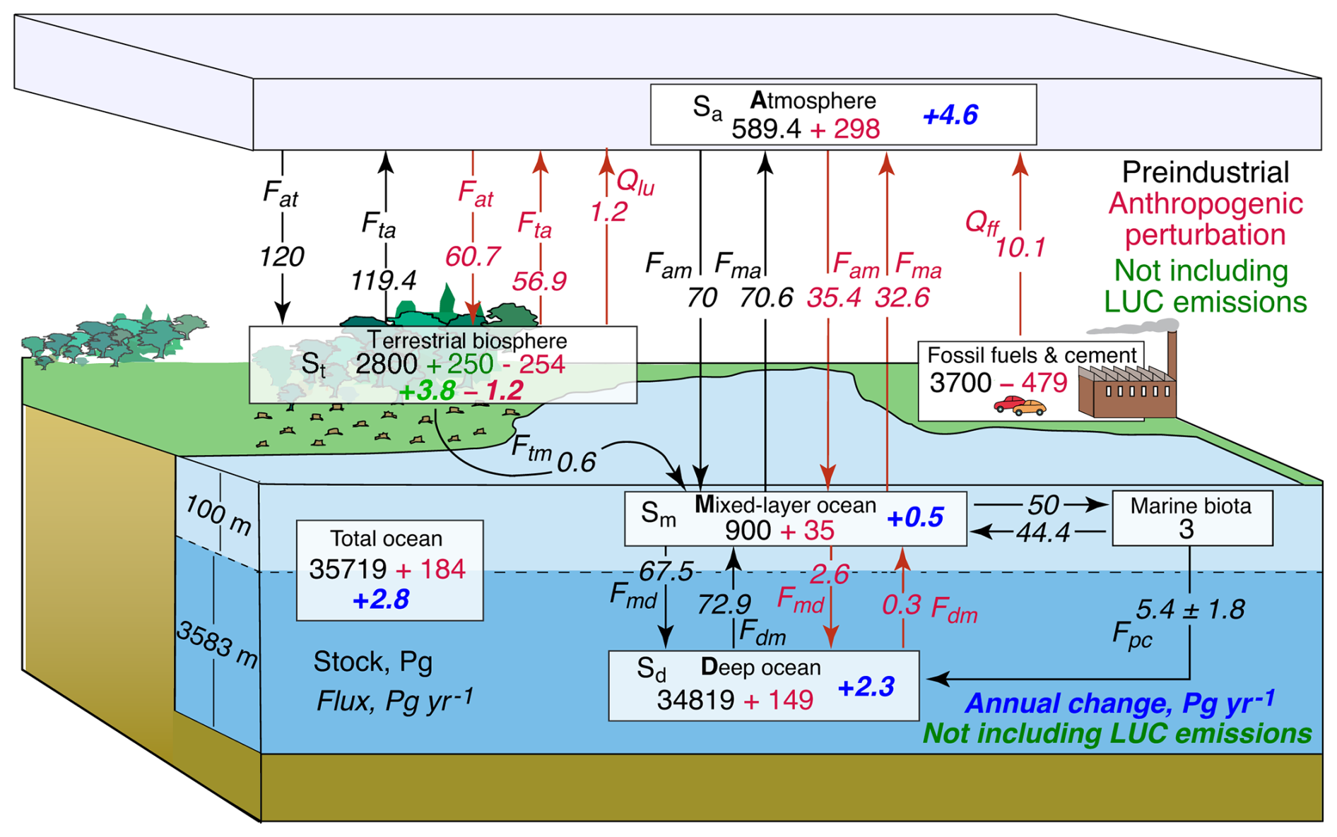
Figure 1 Stocks S_i of carbon in principal compartments that are pertinent to atmospheric CO₂ and fluxes between compartments F_ij in response to concentration-driven forcing by atmospheric CO₂ according to measurements over the Anthropocene. According to the convention introduced by Sarmiento and Gruber (2002), stocks (Pg C) are indicated in roman, and fluxes and annual changes in stocks (Pg C yr⁻¹) are indicated in italics. Preindustrial quantities are given in black, perturbations resulting from anthropogenic emissions are given in red, and present-day annual changes in stocks $\mathrm{d}{S}_i/\mathrm{d}t$ (Pg C yr⁻¹) are given in blue or – excluding land-use change (LUC) emissions – in green. Q_ff and Q_lu denote anthropogenic emissions from fossil fuel combustion (including cement production) and from net land-use change, respectively. The depths of the ML and the DO are shown on the left. The figure is adapted and modified substantially from Fig. 7.3 of AR4 (Denman et al., 2007), with quantities developed here and updated to reflect the early 2020s time frame. Quantities are shown with more precision than is justified by the accuracy with which they are known to allow differencing.

The quantities shown in Fig. 1 are stocks in each of the several compartments S_i and gross (not net) fluxes F_ij (positive in the direction of the arrow), the annual changes in several of the compartments, and anthropogenic emissions Q_ff and Q_lu. Q_lu, the net land-use change (LUC) emission, represents the net annual carbon flux from the TB into the atmosphere due to net deforestation, i.e., the flux from deforestation minus that from afforestation and due to other anthropogenic changes affecting carbon in the terrestrial biosphere, including grasslands, soil carbon, and the like. There are four compartments pertinent to the distribution of anthropogenic CO₂: the atmosphere, the ML, the DO, and the TB. By conservation of matter, the sum of the changes in stocks in those compartments is equal to anthropogenic emissions, all as a function of time over the Anthropocene. Several of the quantities in the figure are little more than guesses, including the preindustrial stocks in the TB and the fossil fuel reserve; current estimates of these quantities vary widely. Other pertinent processes, minor on the centennial timescale examined here, include exchanges of carbon with the ocean through river runoff and loss of atmospheric CO₂ through weathering and sedimentation. For a recent review, see Crisp et al. (2022). These terms of the carbon budget, all of which are small on annual to centennial timescales, are neglected here.

For the PI time, the atmospheric stock is accurately known from measurements. The ML stock is calculated for assumed near equilibrium between the atmosphere and the ML, with the ML depth taken as 100 m; this depth was apparently assumed in previous versions of Fig. 1, but it seems to be explicitly stated only in the predecessor figure shown in AR3 (Prentice et al., 2001). A mean thermocline depth of 75 m, used by several prior investigators, importantly Bolin and Eriksson (1959), appears to derive from an early study by Craig (1957), who reported it as 75 ± 25 m or, equivalently, 2 % of the volume of the global ocean. More recent observational support for the choice of 100 m as an appropriate depth of the ML comes from systematic time series of ocean temperature at sub-annual intervals, as a function of depth gridded to 0.1 year intervals and 10 m vertical resolution, based on systematic measurements along commercial shipping lanes through the high-resolution expendable bathythermograph (HRXBT) project (https://www-hrx.ucsd.edu/index.html, last access: 27 May 2025). For example, the extended data of Sutton and Roemmich (2001), constituting the mean over a section extending north from Auckland, Aotearoa / New Zealand (37 to 30° S; 600 km), over the years 1986–2018, show penetration of heat due to the annual cycle of insolation from the surface to a depth of about 100 m and a sharp maximum in the gradient of temperature with a depth at about 75 to 100 m. These data are plotted in the open discussion of the present paper (https://egusphere.copernicus.org/preprints/2024/egusphere-2024-2893/#AC2, last access: 17 June 2025). Similar conclusions about the penetration of the annual signal can be drawn from other studies in this project (e.g., Wijffels and Meyers, 2004).

The depth of the DO, z_d, is obtained as the difference between the mean depth of the global ocean, 3683 m, and the ML depth. The ML and the DO are assumed to be in steady state (not equilibrium) in the PI period. The departure from equilibrium is manifested by the upward PI flux F_dm that is due to exchange of water between the ML and the DO slightly exceeding the downward flux F_md – this is necessary to account for a gravitational flux of biogenic particulate carbon from the ML to the DO, which contributes to the total downward flux. This “do-nothing” cycle is shown in the figure for completeness, but it plays no role in the analysis here and is neglected in this analysis. The PI flux from the atmosphere to the TB is taken here as being equal to the estimate of gross primary production of Beer et al. (2010), but this quantity is highly uncertain; the reverse flux maintains the PI steady state, with a small riverine flux from the TB into the ML, which is then matched by the slight difference in the PI fluxes between the ML and the atmosphere and is responsible for the slight disequilibrium between the two compartments.

The anthropogenic increments in the several stocks and fluxes are the differences between PD and PI values. The principal objective of the present study is to determine the annual changes in the two ocean compartments, as forced by the annual increment in the atmospheric stock of CO₂, $\mathrm{d}{S}_{\mathrm{a}}/\mathrm{d}t$, which is obtained from measurements. Attention is drawn to the PD rate of increase in the total ocean stock, 2.8 Pg yr⁻¹, which is compared with results from measurements and other modeling studies. Of this total annual increment, the vast majority, 2.3 Pg yr⁻¹, represents an increase in the stock of the DO, making the processes controlling this increment of particular interest. Also shown in Fig. 1, for reference, but not used here, are the emissions from fossil fuel combustion (including cement production) and from land-use change, which sum to 11.3 Pg yr⁻¹. The difference between this total annual emission and the sum of the annual increments in the atmosphere, the ML, and the DO is the annual increment in the TB, 3.8 Pg yr⁻¹. In constructing the budget shown in Fig. 1, the anthropogenic flux from the atmosphere to the TB is assumed to scale linearly with the atmospheric CO₂ stock; the reverse flux is less than the forward flux as a consequence of uptake of anthropogenic carbon by the TB. It should be stressed that the fluxes between the atmosphere and the TB shown in the figure are little more than guesstimates, which are presented to give a rough sense of their magnitudes. These fluxes themselves are not important in this study; rather, it is the net fluxes that are important, and, as noted, those fluxes are not actively modeled here but are determined by the difference between emissions and actively modeled quantities.

The objective of the present study is to develop and apply a three-compartment concentration-driven model (denoted 3C-CDM) to represent the processes governing the evolution of the system shown in Fig. 1. As noted, for example, by Melnikova et al. (2023), by ensuring consistent CO₂ amounts across models, concentration-driven simulations readily allow consistent comparison of carbon cycle processes across different models. The variables included in the 3C-CDM are time-dependent global stocks of CO₂ in the atmosphere, and DIC in the ML and DO, all expressed as carbon mass. The measured stock of atmospheric CO₂ is used as a forcing in the set of ordinary differential equations describing the evolution of the system. The stock in the TB is not actively modeled but is evaluated, mainly for reference, as the residual between time-dependent integrated anthropogenic emissions and the anthropogenic stocks in the other three compartments. Hence, the stocks in the ML and the DO are the only actively modeled quantities. The model requires four parameters: the four transfer coefficients describing rates of transfer between the atmosphere and the ML and between the ML and the DO. However, because it is the same processes that drive exchange in opposite directions, the number of required independent parameters is reduced to two. Use of a concentration-driven model readily allows examination of the sensitivity to model structure, to parameter values, and to the time-dependent distribution of anthropogenic carbon in the receiving compartments. Importantly, in the concentration-driven model it is possible to readily compare the full model, in which stocks in both the ML and the DO are actively modeled, with an equilibrium variant of the model, in which the stock in the ML is treated as being in equilibrium with that in the atmosphere. Treating the atmosphere and the ML as a single concentration-driven compartment closely reproduces the results obtained with the stock in the ML being actively modeled, a manifestation of near equilibrium between the two compartments; such treatment reduces the number of receiving compartments to one, the DO, and thereby reduces the number of independent parameters to one.

In the model, the stocks, gross fluxes, and transfer coefficients are related as

$$\begin{array}{}\text{(1)}& F_{ij}=k_{ij}{S}_i.\end{array}$$

The transfer coefficients are taken as constant over the industrial period, except for the transfer coefficient from the ML to the atmosphere, k_ma, the value of which depends on the amount of DIC in the ML, through well-understood equilibria in the carbon dioxide–bicarbonate–carbonate system. As developed in Sect. 3, the transfer coefficients are constrained by rather well-characterized and independently measured rates of exchange of material or heat between compartments – an air–sea gas exchange coefficient that is more or less universal for low- to medium-solubility gases – and by the measured rate of heat uptake by the global ocean over the past several decades, yielding transfer coefficients coupling the ML and the DO. From an inspection of Fig. 1 it becomes apparent that the most important transfer coefficient is that governing transfer from the ML to the DO, k_md; the reverse transfer coefficient k_dm is of secondary importance, simply because the reverse upward flux is an order of magnitude smaller than the forward downward flux. Hence, much attention is given here to the determination of k_md. The transfer coefficients between the atmosphere and the ML are of relatively minor importance to the evolution of the system because of the near-equal and opposite anthropogenic fluxes, indicative of near equilibrium between the compartments, even under continuing anthropogenic perturbation. In fact, as noted above and shown in Sect. 5, there is little change in the budget even if the ML is assumed to be in equilibrium with the atmosphere, showing insensitivity to the transfer coefficients.

3 Transfer coefficients

This section develops the transfer coefficients between the ML and the DO and between the atmosphere and the ML.

3.1 Transfer between the ML and the DO

Transfer of tracers between the ML and the DO is a physical process, the rate of which is governed by the rate of water volume (or mass) exchange between the two compartments; the tracer just goes along for the ride. The amount of the tracer that is in the compartment with a higher concentration is diminished by this exchange, and the amount of tracer in the compartment with a lower concentration is augmented by this exchange. The fractional rate of exchange relative to the stock in the leaving compartment, k_ij, is equal to the rate of volume exchange F_V (dimension L³ T⁻¹), divided by the volume V_i (dimension L³) of the leaving compartment, and is thus of dimension T⁻¹.

$$\begin{array}{}\text{(2)}& k_{ij}={\displaystyle \frac{\left(\frac{\partial S_i}{\partial t}\right)}{S_i}}={\displaystyle \frac{F_{\mathrm{v}}}{V_i}}\end{array}$$

Here, the partial derivative refers to the rate of change due only to the exchange process. The rate of volume exchange F_V may be viewed as an area (here the area of the global ocean, A_O, dimension L²) times a velocity (dimension L T⁻¹), denoted here as piston velocity v_p. Similarly, the volume itself is the product of the area times the depth, z_i. Hence

$$\begin{array}{}\text{(3)}& k_{ij}={\displaystyle \frac{\left(\frac{\partial S_i}{\partial t}\right)}{S_i}}={\displaystyle \frac{F_{\mathrm{v}}}{V_i}}={\displaystyle \frac{v_{\mathrm{p}}{A}_{\mathrm{O}}}{A_{\mathrm{O}}{z}_i}}={\displaystyle \frac{v_{\mathrm{p}}}{z_i}}.\end{array}$$

In other words, $k_{\mathrm{md}}/z_{\mathrm{m}}$ and $k_{\mathrm{dm}}=v_{\mathrm{p}}/z_{\mathrm{d}}$. The question is thus how to obtain an independent measure of v_p based on some tracer other than CO₂ to avoid circular reasoning.

The piston velocity quantifying the rate of transfer of water and, by extension, of any tracer between the ML and the DO is of great importance here and in many geophysical applications. An early determination of this quantity, 3 to 3.5 m yr⁻¹, was obtained from the difference in the ratio of ¹⁴CO₂ to ¹²CO₂ in the upper ocean versus that in the DO, using the half-life of ¹⁴CO₂ as a clock (Broecker and Peng, 1982, pp. 236–243; also Sarmiento and Gruber, 2006, hereinafter SG06, p. 12). Using a global inverse model, DeVries et al. (2017) quantified temporal variations in basinwide and global-scale volume exchange rates between the ML and the DO, finding global mean volume exchange rates of 57, 72, and 49 Sv for the 1980s, 1990s, and 2000s, respectively (where Sv, or Sverdrup, is the flow rate in units of 10⁶ m³ s⁻¹). Expressed as piston velocity, as used here, these correspond to 4.98, 6.29, and 4.28 m yr⁻¹, respectively. The piston velocity, as employed here, should not be confused with the quantity, also denoted in the same manner as piston velocity, characterizing the rate of diffusive transfer of a dissolved gas through the stagnant film between the air–ocean interface and the turbulent region away from the interface (SG06, p. 82).

The approach taken here comes from the recognition that the piston velocity governing the exchange of CO₂ between the ML and the DO is the same as that governing the flux of heat energy from the ML to the DO, which has been induced by the increase in global mean surface temperature over the Anthropocene era, especially given the similar time history of these perturbations. The basis for the determination of the flux between the ML and the DO in the present study is the measured rate of heat uptake by the global ocean in response to the increase in global temperature over the past 50 years. The so-called “nexus” between uptake of heat and CO₂ by the global ocean was highlighted in the IPCC Sixth Assessment Report (Monteiro et al., 2021), which calls attention to the commonality of the transport processes that govern ocean uptake of excess CO₂ and heat. Bronselaer and Zanna (2020) found a linear relation between the increase in the heat content in the global ocean, as determined by direct measurement, and the increase in global DIC, obtained by an inverse carbon cycle model based on assimilation of potential temperature, salinity, radiocarbon, and CFC-11 observations (DeVries, 2014); the data presented by Bronselaer and Zanna (2020) for the time period of 1965–2017 exhibit a remarkably high coefficient of determination (r²) of 0.991 between excess heat and excess ocean carbon stock. Although that relation cannot be used to obtain a measure of the transfer flux between the ML and the DO, because it deals with total ocean heat content rather than the ML and DO separately and because the developed relation characterizes the response of ocean heat content to all forcings, not just CO₂ forcing, the tight relation shown in that study lends strong support to the approach taken here of using the rate of heat transfer from the ML to the DO, together with the increase in global mean surface temperature, to determine the piston velocity pertinent to the transfer of any tracer, importantly including DIC, between the two compartments.

Figure 2 shows the several quantities needed to evaluate the rate of increase in the heat content of the global ocean per increase in global temperature anomaly:

$$\begin{array}{}\text{(4)}& {\mathit{\kappa }}_H={\displaystyle \frac{\mathrm{d}\frac{\mathrm{d}{H}_{\mathrm{O},\mathrm{tot}}}{\mathrm{d}t}}{\mathrm{d}T}},\end{array}$$

where H_O,tot denotes the heat content anomaly of the total global ocean, that is, the sum of the anomalies for the ML and the DO. Figure 2a shows a roughly linear increase in global mean surface temperature (GMST) anomaly (ΔT; GISTEMP Team, 2024) with time over the period of 1960 to the present. Figure 2b shows the increase in global ocean heat content ΔH_O,tot over the same time period, as presented in a recent review of observational data by Cheng et al. (2024). Figure 2c shows the time derivative of ΔH_O,tot, d$H_{\mathrm{O},\mathrm{tot}}/\mathrm{d}t$; like GMST, d$H_{\mathrm{O},\mathrm{tot}}/\mathrm{d}t$ exhibits a linear increase with time. The slope of the fit in Fig. 2d of d$H_{\mathrm{O},\mathrm{tot}}/\mathrm{d}t$ vs. T gives the desired quantity κ_H, having a value of 13.8 ± 3.2 ZJ yr⁻¹ K⁻¹, which is equivalent to 1.20 ± 0.28 W m⁻² K⁻¹. Throughout this paper, uncertainties are given as 1σ. This slope exhibits considerable uncertainty of 24 %, a manifestation of the rather large fluctuations in d$H_{\mathrm{O},\mathrm{tot}}/\mathrm{d}t$ shown in Fig. 2c and a that are due mainly to fluctuations in reported values of ΔH_O,tot (Fig. 2b). Those fluctuations may be actual fluctuations in this quantity occurring on a timescale of a few years (as with ΔT) or may be artifacts arising from errors in the measurements themselves, from inadequacies in spatial coverage, or both.

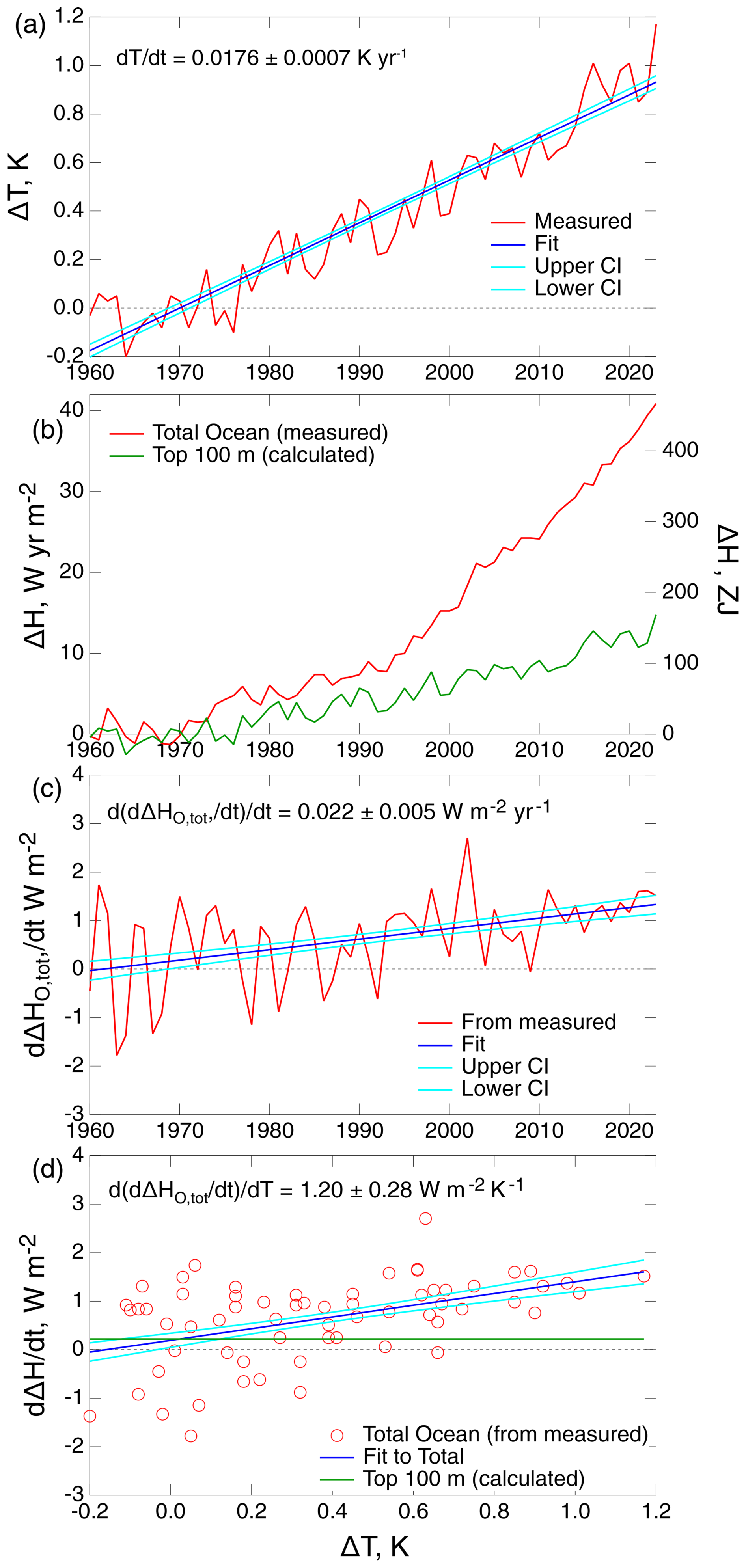
Figure 2 Time dependence of quantities required to quantify uptake of heat by the global ocean over the years 1960–2023. (a) Global mean surface temperature anomaly ΔT (GISTEMP Team, 2024). (b) Heat content anomaly of the global ocean ΔH_O,tot, referenced to 1960, from the assessment of measurements by Cheng et al. (2024) and as calculated for the top 100 m of the global ocean, ΔH_ML, for assumed thermal equilibrium with global temperature anomaly ΔT. The right-hand scale gives ΔH in systematic (SI) units, as employed by Cheng et al. (2024), where the prefix Z denotes 10²¹; the left-hand scale gives ΔH in units that are more readily related to the energy budget of the global ocean per area of the global ocean A_O. (c) Time derivative $\mathrm{d}\mathrm{\Delta }{H}_{\mathrm{O},\mathrm{tot}}/\mathrm{d}t$, based on measured ΔH_O,tot. (d) Time derivatives $\mathrm{d}\mathrm{\Delta }{H}_{\mathrm{O},\mathrm{tot}}/\mathrm{d}t$ and $\mathrm{d}\mathrm{\Delta }{H}_{\mathrm{ML}}/\mathrm{d}t$ in conventional units, as in (c), plotted against ΔT. Confidence band (68 % CI) and fitting coefficients (68 % CI) are shown with the fits.

The total ocean heating rate is the sum of two components, the heating rate of the ML and the heating rate of the DO, with the latter corresponding to the transfer flux of heat from the mixed-layer ocean to the deep ocean:

$$\begin{array}{}\text{(5)}& {\displaystyle \frac{\mathrm{d}\frac{\mathrm{d}{H}_{\mathrm{O},\mathrm{tot}}}{\mathrm{d}t}}{\mathrm{d}T}}={\displaystyle \frac{\mathrm{d}\frac{\mathrm{d}{H}_{\mathrm{m}}}{\mathrm{d}t}}{\mathrm{d}T}}+{\displaystyle \frac{\mathrm{d}\frac{\mathrm{d}{H}_{\mathrm{d}}}{\mathrm{d}t}}{\mathrm{d}T}},\end{array}$$

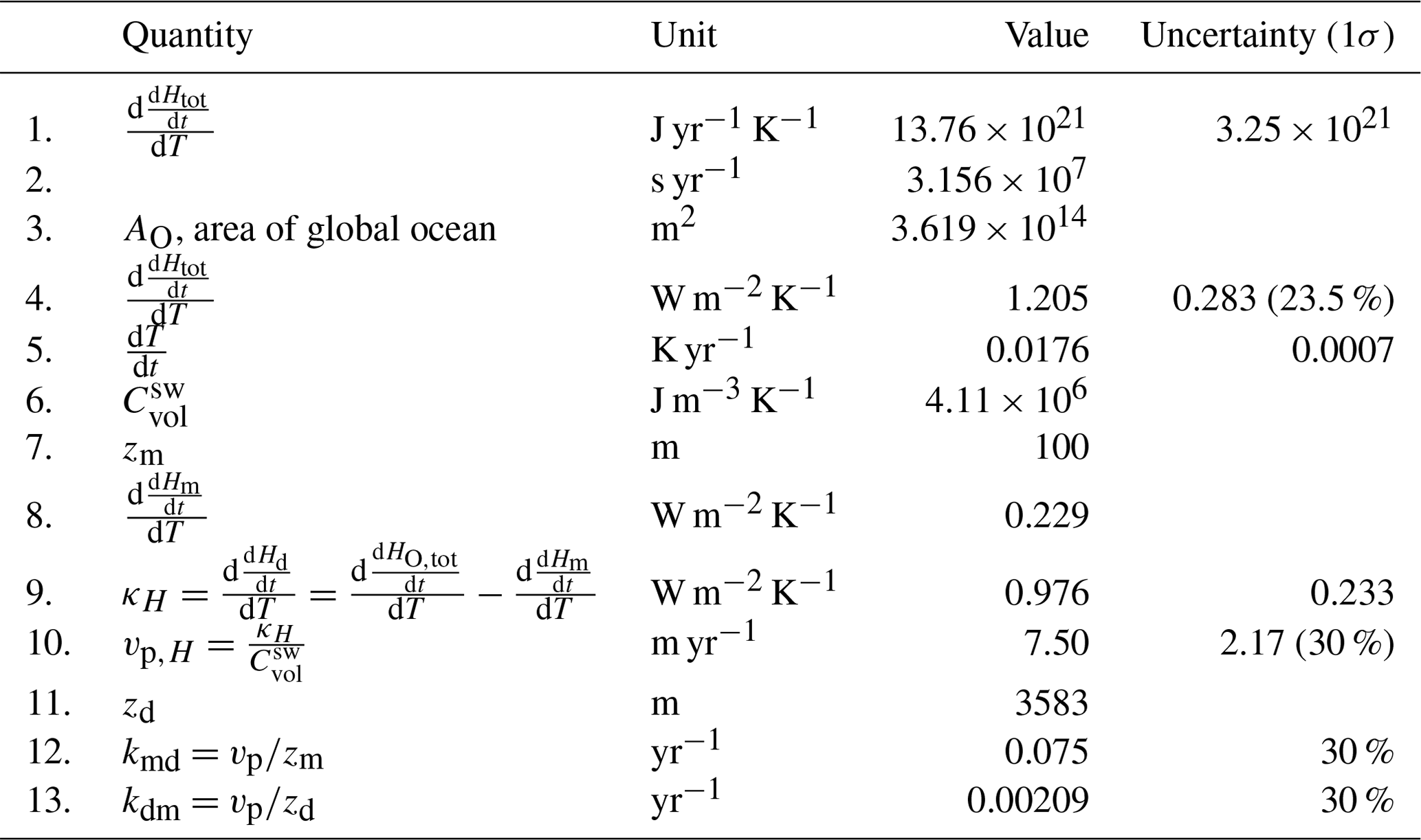
where the second term on the right is the quantity of principal interest here, used to obtain the piston velocity pertinent to the transfer of tracers from the ML to the DO. Table 1 outlines the calculations leading to the evaluation of this piston velocity. In customary units, $\mathrm{d}\left(\mathrm{d}{H}_{\mathrm{O},\mathrm{tot}}/\mathrm{d}t\right)/\mathrm{d}T=$ 1.207 W m⁻² K⁻¹, referred to the area of the global ocean (row 4 of Table 1). The rate of increase in the heat content of the ML is evaluated as the rate of increase in global temperature times the heat capacity of the ML (z_m times the volumetric heat capacity of seawater, $C_{\mathrm{vol}}^{\mathrm{sw}}$):

$$\begin{array}{}\text{(6)}& {\displaystyle \frac{\mathrm{d}{H}_{\mathrm{m}}}{\mathrm{d}t}}={\displaystyle \frac{\mathrm{d}{T}_{\mathrm{m}}}{\mathrm{d}t}}{C}_{\mathrm{vol}}^{\mathrm{sw}}{z}_{\mathrm{m}}.\end{array}$$

(Here the assumption of thermal equilibrium between the ML and the atmosphere is not required but only the weaker assumption that the rate of increase in temperature is the same for both compartments.) For d$T_{\mathrm{m}}/\mathrm{d}t$ = 0.0176 ± 0.0007 K yr⁻¹ (Fig. 2a), $C_{\mathrm{vol}}^{\mathrm{sw}}=$ 4.11×10⁶ J m⁻³ K⁻¹, and z_m again taken as 100 m, $\mathrm{d}\left(\mathrm{d}{H}_{\mathrm{ML}}/\mathrm{d}t\right)/\mathrm{d}T=$ 0.229 W m⁻² (row 8). This quantity must be subtracted from the total $\mathrm{d}\left(\mathrm{d}{H}_{\mathrm{O},\mathrm{tot}}/\mathrm{d}t\right)/\mathrm{d}T$ to yield the increase in deep ocean heating per increase in GMST, ${\mathit{\kappa }}_H=\mathrm{d}\left(\mathrm{d}{H}_{\mathrm{DO}}/\mathrm{d}t\right)/\mathrm{d}T=$ 0.976 W m⁻² K⁻¹, a quantity that is of broad geophysical interest beyond its application here. In turn, the piston velocity, which is related (row 10) to the heat transfer coefficient as

$$\begin{array}{}\text{(7)}& v_{\mathrm{p},H}={\mathit{\kappa }}_H/C_{\mathrm{vol}}^{\mathrm{sw}},\end{array}$$

is 7.50 m yr⁻¹, or ± 30 % 1σ. The piston velocity determined in this way from measurements of the heating rate of the global ocean provides an independent, observationally based measure of this quantity (which is similarly of broad geophysical interest) that can be used with confidence in determining components of the global CO₂ budget. The corresponding transfer coefficients are

$$\begin{array}{}\text{(8)}& \begin{array}{rl}& k_{\mathrm{md}}=v_{\mathrm{p}}/z_{\mathrm{m}}=\mathrm{0.075}{\mathrm{yr}}^{-\mathrm{1}}\mathrm{and}\\ & k_{\mathrm{dm}}=v_{\mathrm{p}}/z_{\mathrm{d}}=\mathrm{0.0021}{\mathrm{yr}}^{-\mathrm{1}},\end{array}\end{array}$$

both likewise uncertain to ± 30 %.

Table 1 Evaluation of piston velocity and transfer coefficients between the mixed-layer ocean and deep ocean.

The values of the transfer coefficients k_md and k_dm obtained in this analysis can be compared to values inferred from the budgets depicted in versions of Fig. 1 presented in recent IPCC assessment reports, as shown in Table 2. Here the values of k_md and k_dm are obtained from the preindustrial stocks and gross fluxes shown in the indicated figures in the several assessment reports by inversion of Eq. (2), specifically for the preindustrial fluxes between the ML and the DO, as

$$\begin{array}{}\text{(9)}& k_{\mathrm{md}}=F_{\mathrm{md}}^{\mathrm{pi}}/S_{\mathrm{m}}^{\mathrm{pi}}\mathrm{and}{k}_{\mathrm{dm}}=F_{\mathrm{dm}}^{\mathrm{pi}}/S_{\mathrm{d}}^{\mathrm{pi}}.\end{array}$$

Also shown in Table 2 are the piston velocities obtained from the transfer coefficients obtained by inversion of Eq. (8). The PI stocks and fluxes are essentially unchanged between the 2007 and 2013 reports. Values of v_p inferred from the fluxes presented in these reports, 10 m yr⁻¹, are somewhat greater than those inferred here, 7.5 ± 2.2 m yr⁻¹. In contrast, the value for v_p given in the 2021 report is a factor of 2.9 higher than the values in the earlier IPCC reports. This value, which cannot be correct, would seem to result from a misreading of a single paper by the authors of the pertinent chapter of AR6. The values and uncertainty range for v_p obtained here are used in the model calculations presented here. As seen in Sect. 5, in the examination of the sensitivity of modeled stock in the DO to uncertainty in piston velocity, a greater piston velocity, such as that inferred from AR4 and AR5, relative to that determined here, would result in a greater modeled stock in the DO over the Anthropocene, relative to that determined here, by about 30 %.

Table 2 Transfer coefficients and piston velocities between the mixed-layer ocean and the deep ocean inferred from recent IPCC assessment reports and determined in this study.

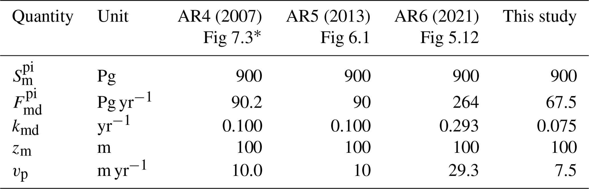
^* Identical values for Sarmiento and Gruber (2002).

Here it should be underscored that the fundamental measure of the rate of transfer of DIC from the ML to the DO (or from the DO to the ML) is the flux. The transfer coefficient k_md is inversely proportional to z_m, whereas the stock in the ML is proportional to z_m (specifically S_m=C_mz_mA_O). Both C_m, the concentration of DIC in the ML, and A_O are independent of z_m. Hence,

$$\begin{array}{}\text{(10)}& F_{\mathrm{md}}=k_{\mathrm{md}}{S}_{\mathrm{m}}={\displaystyle \frac{v_{\mathrm{p}}}{z_{\mathrm{m}}}}{C}_{\mathrm{m}}{z}_{\mathrm{m}}{A}_{\mathrm{O}}=v_{\mathrm{p}}{C}_{\mathrm{m}}{A}_{\mathrm{O}},\end{array}$$

from which it is seen that the piston velocity, not the transfer coefficient, is the fundamental parameter governing the fluxes between the ML and the DO.

3.2 Transfer coefficients coupling the atmosphere and ML

3.2.1 Transfer from the atmosphere to the ML

Gas exchange from the atmosphere to the ML for all low- to medium-solubility gases, being controlled by mass transport on the water side of the atmosphere–ocean interface, is governed by the same physics, namely turbulent transfer. (For higher-solubility gases, the mass transport rate is increasingly influenced by the rate of turbulent transfer in the atmosphere; Schwartz, 1992.) The gross (one-way, not net) mass transport flux of a soluble gas, φ, between the gaseous and aqueous phases is related to the concentration on the leaving side as

$$\begin{array}{}\text{(11)}& {\mathit{\varphi }}_{ij}=v_{ij}{c}_i,\end{array}$$

where φ_ij is the gross flux from phase i to phase j with a dimension of an amount (or mass) per area and time, c_i denotes the concentration on the leaving side as the amount or mass concentration, and v_ij is a mass transfer coefficient (dimension L T⁻¹). Because of this dimension, the mass transfer coefficient is commonly denoted as a velocity.

The water-side mass transfer coefficient v_ma depends strongly on turbulent mixing, which, in turn, in the atmosphere–ocean environment depends on the rate of turbulent mixing on the water side. The diffusivity of the dissolved gas in seawater plays a less important role in the rate of mass transfer. The greater the diffusion coefficient, the greater the transfer coefficient. These dependences have been thoroughly studied in the laboratory and the ocean environment and are rather well characterized and understood (e.g., SG06). Because the controlling physics is the same for all gases, the water-side mass transfer coefficient characterizing the transport of low- to medium-solubility gases into seawater can be considered a more or less universal quantity, albeit one that is not precisely known. SG06 examine laboratory studies and field measurements, e.g., with the long-lived (5730-year half-life) isotopic variant of CO₂ and ¹⁴CO₂ and short-lived (3.8 d) ²²²Rn. Multiple formulations give comparable values and wind speed dependence. For CO₂, SG06 conclude that, for the preindustrial mixing ratio of CO₂ and suitable global mean temperature and ocean salinity (SG06), the global annual mean gas exchange velocity for water-side mass transport of CO₂, expressed in terms of the concentration of CO₂ (not DIC) on the water side of the interface, is about 17 cm h⁻¹; the corresponding transport coefficient representing the gross flux, not the net flux, which would depend on the difference between the concentrations in the two phases. The several prior studies compared by SG06 give values of v_ma that range from 11.2 to 18.7 cm h⁻¹. These estimates result from averages of local and instantaneous transfer velocity, a quantity that depends strongly on wind speed (roughly as the second power) and, to lesser extent, on other situational variables (e.g., Liss and Merlivat, 1986; Takahashi et al., 2009; Wanninkhof et al., 2013).

To evaluate the gross flux from the atmosphere to the ocean, it is desirable to express the mass transport coefficient in terms of gas-phase CO₂ concentration and, ultimately, the atmospheric CO₂ stock. The transfer coefficient between the atmosphere and the ML, referred to the gas-phase CO₂ concentration (v_am), is related to the transport coefficient between the two compartments, referred to the aqueous-phase CO₂ concentration (v_ma), by the dimensionless volumetric Henry's law solubility coefficient $H_{\mathrm{s}}^{\mathrm{cc}}$. Here the notation of Sander et al. (2022) is used, where the subscript s denotes solubility (aqueous per gas, to distinguish it from volatility, gas per aqueous), and the superscripts c refer to concentration (amount per volume, to distinguish it from the mixing ratio, mole fraction, and other units) in the two phases (aqueous concentration per gas concentration), as (e.g., Liss and Slater, 1974; Schwartz, 1992)

$$\begin{array}{}\text{(12)}& v_{\mathrm{am}}=v_{\mathrm{ma}}{H}_{\mathrm{s}}^{\mathrm{cc}}.\end{array}$$

For CO₂, $H_{\mathrm{s}}^{\mathrm{cc}}$ is near unity (0.83 at 291 K; Weiss, 1974; Lewis and Wallace, 1998). For v_ma, taken as 17 cm h⁻¹, the resulting global and annual mean value of v_am is 14.2 cm h⁻¹, again with an uncertainty of ± 30 %. Converting to conventional units and taking into account the area of the global ocean A_O (3.619×10¹⁴ m²; Eakins and Sharman, 2012) and the volume of the atmosphere V_A,

$$\begin{array}{}\text{(13)}& k_{\mathrm{am}}={\displaystyle \frac{A_{\mathrm{O}}}{V_{\mathrm{A}}}}{v}_{\mathrm{am}},\end{array}$$

where V_A is evaluated from the number of moles in the global atmosphere 1.765×10²⁰ mol (Prather et al., 2012) and yields the transfer coefficient k_am= 0.107 yr⁻¹. This value is essentially the same as that which can be inferred from the ratio of preindustrial $F_{\mathrm{am}}/S_{\mathrm{a}}$ given in the predecessor figure to Fig. 1 (Sarmiento and Gruber, 2002), 0.119 yr⁻¹, which evidently results from similar reasoning. Estimates of k_am, as inferred from recent IPCC assessment reports, have varied slightly (see Table 3). Here the value k_am= 0.119 yr⁻¹ from Sarmiento and Gruber (2002) is retained to avoid the proliferation of values; as shown in Sect. 5, the evolution of DIC over the industrial period is quite insensitive to the value of k_am, so the range of values of k_am given in Table 3 is of little consequence. The transfer coefficient k_am, being an intensive quantity, denoting the global and annual mean gross transfer rate of CO₂ from the atmosphere to the surface ocean divided by the amount of CO₂ in the global atmosphere, is independent of the amount of CO₂ in the atmosphere and the amount or concentration of dissolved CO₂ in the ocean. The resulting gross flux from the atmosphere to the ML,

$$\begin{array}{}\text{(14)}& F_{\mathrm{am}}=k_{\mathrm{am}}{S}_{\mathrm{a}},\end{array}$$

scales linearly with the atmospheric stock.

Table 3 Atmosphere–ocean transfer coefficient (deposition velocity) for CO₂ inferred from recent assessments.

3.2.2 Transfer from the ML to the atmosphere

For the transfer of CO₂ from the ML to the atmosphere, the situation is considerably more complicated because the substance that crosses the interface is CO₂, whereas the dissolved substance, the stock of which is the modeled quantity, consists of a mixture of hydrated CO₂ and bicarbonate (mainly) and carbonate ions, collectively denoted dissolved inorganic carbon (DIC). The dissociation equilibria relating the concentrations of these species are well characterized and understood (e.g., SG06), with the effect that the solubility of CO₂ in seawater and the transfer coefficient characterizing the rate of transfer of DIC from seawater to the atmosphere are dependent on pH or, alternatively, on the stock of DIC in the ML. In the model developed here, it is desired to express the fluxes in both directions in terms of the stocks. This situation is readily dealt with using well-established equilibrium relations between concentrations of DIC and CO₂(aq) but has the consequence that the transfer coefficient k_ma is dependent on the concentration of DIC and is thus not a constant in the same sense as k_am. The approach taken here is developed in Appendix B. Summarizing the results of the derivation given there, the return flux from the ML to the atmosphere is given in terms of the transfer coefficient for the forward flux k_am times the stock in the ML S_m and a differential equilibrium constant $K{{}^{\prime }}_{\mathrm{ma}}(S_{\mathrm{m}}$), where the dependence on S_m is explicitly noted as

$$\begin{array}{}\text{(15)}& F_{\mathrm{ma}}\left(S_{\mathrm{m}}\right)=k_{\mathrm{am}}\cdot K{{}^{\prime }}_{\mathrm{ma}}\left(S_{\mathrm{m}}\right)S_{\mathrm{m}},\end{array}$$

where

$$\begin{array}{}\text{(16)}& K{{}^{\prime }}_{\mathrm{ma}}\left(S_{\mathrm{m}}\right)={\left({\displaystyle \frac{\mathrm{d}{S}_{\mathrm{a}}}{\mathrm{d}{S}_{\mathrm{m}}}}\right)}_{\mathrm{eq}}.\end{array}$$

Defining an effective transfer coefficient $k{{}^{\prime }}_{\mathrm{ma}}$,

$$\begin{array}{}\text{(17)}& F_{\mathrm{ma}}\left(S_{\mathrm{m}}\right)=k{{}^{\prime }}_{\mathrm{ma}}{S}_{\mathrm{m}},\end{array}$$

then

$$\begin{array}{}\text{(18)}& k{{}^{\prime }}_{\mathrm{ma}}=F_{\mathrm{ma}}\left(S_{\mathrm{m}}\right)/S_{\mathrm{m}}=k_{\mathrm{am}}\cdot K{{}^{\prime }}_{\mathrm{ma}}\left(S_{\mathrm{m}}\right).\end{array}$$

Noting that

$$\begin{array}{}\text{(19)}& {\left({\displaystyle \frac{\mathrm{d}{S}_{\mathrm{a}}}{\mathrm{d}{S}_{\mathrm{m}}}}\right)}_{\mathrm{eq}}={\displaystyle \frac{V_{\mathrm{A}}}{A_{\mathrm{O}}{z}_{\mathrm{m}}{H}_{\mathrm{s}}^{\mathrm{cc}}}}{\displaystyle \frac{\mathrm{d}\left[{\mathrm{H}}_{\mathrm{2}}{\mathrm{CO}}_{\mathrm{3}}\right]}{\mathrm{d}\left[\mathrm{DIC}\right]}},\end{array}$$

then

$$\begin{array}{}\text{(20)}& K{{}^{\prime }}_{\mathrm{ma}}\left(S_{\mathrm{m}}\right)={\displaystyle \frac{V_{\mathrm{A}}}{A_{\mathrm{O}}{z}_{\mathrm{m}}{H}_{\mathrm{s}}^{\mathrm{cc}}}}{\displaystyle \frac{\mathrm{d}\left[{\mathrm{H}}_{\mathrm{2}}{\mathrm{CO}}_{\mathrm{3}}\right]}{\mathrm{d}\left[\mathrm{DIC}\right]}},\end{array}$$

and in turn

$$\begin{array}{}\text{(21)}& k{{}^{\prime }}_{\mathrm{ma}}=k_{\mathrm{am}}{\left({\displaystyle \frac{\mathrm{d}{S}_{\mathrm{a}}}{\mathrm{d}{S}_{\mathrm{m}}}}\right)}_{\mathrm{eq}}=k_{\mathrm{am}}{\displaystyle \frac{V_{\mathrm{A}}}{A_{\mathrm{O}}{z}_{\mathrm{m}}{H}_{\mathrm{s}}^{\mathrm{cc}}}}{\displaystyle \frac{\mathrm{d}\left[{\mathrm{H}}_{\mathrm{2}}{\mathrm{CO}}_{\mathrm{3}}\right]}{\mathrm{d}\left[\mathrm{DIC}\right]}}.\end{array}$$

This expression is used in the differential equations that describe the evolution of the system in response to the concentration-driven forcing.

4 Historical atmospheric CO₂, preindustrial stocks, and emissions

4.1 Atmospheric CO₂

The 3C-CDM is driven by observed atmospheric CO₂ stock, S_a, obtained from the global mean mixing ratio of atmospheric CO₂ by the conversion factor 2.120 Pg ppm⁻¹. Here the atmospheric mixing ratio of CO₂, $x_{{\mathrm{CO}}_{\mathrm{2}}}$, is taken as the integral of the annual growth rate of the CO₂ mixing ratio presented in the historical tab of the data table accompanying the 2023 Global Carbon Budget (Friedlingstein et al., 2023; GCB23). Values of $x_{{\mathrm{CO}}_{\mathrm{2}}}$ in the earlier part of the modeled period (1750–2022) were obtained from measurements in air trapped in ice in time-resolved cores taken in Antarctica, and in the later part of the period (subsequent to 1959) they were obtained from direct measurements of CO₂ in air, initially at Mauna Loa and the South Pole and subsequently at multiple locations. The several measurement data sets, which are in close agreement during the overlap periods, can be used with high confidence. Preindustrial $x_{{\mathrm{CO}}_{\mathrm{2}}}$ was taken as 278 ppm in the year 1750. The time-dependent anthropogenic atmospheric stock $S_{\mathrm{a}}^{\mathrm{ant}}\left(t\right)$ is obtained as the difference $S_{\mathrm{a}}\left(t\right)-S_{\mathrm{a}}^{\mathrm{pi}}$.

4.2 Preindustrial stocks

Preindustrial stocks are required to initiate the model. In principle, if the system were linear, the modeled quantities could be the anthropogenic perturbations to the stocks, all initiated as 0. However, as noted, the equilibrium solubility of CO₂ in seawater is nonlinear, depending on the amount of DIC in the seawater, and this nonlinear dependence of CO₂ solubility must be accounted for in the model. The nonlinearity is dramatically illustrated by the values of the stocks shown in Fig. 1. In the preindustrial state, the ratio of DIC in the ML to atmospheric CO₂ is 900$/$589.4, or roughly 1.5. In contrast, for the anthropogenic increment, the ratio is 35$/$298, or roughly 0.12, which is more than an order of magnitude less. Hence, it is necessary to use actual measured CO₂ to drive the model and to calculate the anthropogenic stock in the ML as the difference between the calculated ML stock and the PI ML stock, taken here as the stock that would be in equilibrium with the PI atmospheric stock.

The PI stock in the ML is in near equilibrium with the stock in the atmosphere. Under PI conditions, these two compartments would be in equilibrium except for a slight departure that is due to uptake of carbon by the TB that is delivered to the ML by riverine fluxes, resulting in a slight excess of DIC in the ML above its value that would be in equilibrium with the atmosphere. This non-equilibrium situation under PI conditions is neglected here as it does not affect anthropogenic stocks and fluxes examined in this model, but the associated net PI flux (0.6 Pg yr⁻¹, Fig. 1) must be taken into account when comparing calculations to measurements. A second departure from equilibrium under PI conditions, also neglected here, is due to particulate carbon produced from biological activity sinking from the ML to the DO. There, it is oxidized and ultimately returned to the ML via exchange of water between the two compartments, resulting in the concentration of DIC in the DO being greater than that in the ML, an effect that is again neglected here. However, this model explicitly evaluates the net transfer of anthropogenic DIC from the ML to the DO that occurs by exchange of water between the two compartments, using the coefficients characterizing the exchange between the two compartments (mainly from the ML to the DO) developed in Sect. 3.

Because of nonlinearity in the relation between DIC in the ML and atmospheric CO₂ stock, the model explicitly calculates total ML DIC stock rather than anthropogenic stock; time-dependent anthropogenic CO₂ stock is evaluated as the difference between modeled total DIC and PI DIC. Anthropogenic stock in the DO is set to zero at the initiation of the model run, and because the exchange between the ML and DO is linear in stocks, the model simply calculates anthropogenic stock directly from the net exchange between the two compartments.

4.3 Emissions

Although anthropogenic emissions are not required to drive the 3C-CDM, they provide context for the fraction of emissions that is present in the atmosphere (determined by measurement), the fraction taken up by the global ocean (as modeled here and by others and substantiated by a few measurements), and the fraction taken up by the terrestrial biosphere (obtained by difference). Historical anthropogenic emissions over the Anthropocene consist of the sum of emissions from fossil fuel combustion (including cement production) and land-use change emissions. The GCB23 data file presents LUC emissions only from 1850 onward, by which time these emissions were already substantial and, in fact, substantially greater than fossil fuel emissions. In the absence of reported emissions prior to 1850, in the present study emissions between 1750 and 1850 were taken as a linear interpolation between 0 in 1750 and the GCB23 value in the year 1850 (0.72 Pg yr⁻¹). This results in a slightly greater value of integrated emissions in the present study than that given by GCB23. These data are also shown in Sect. 5.

5 Model and results

The model developed and presented here consists of a set of two coupled ordinary differential equations in the stocks in the ML and the DO. The model is forced by the increasing values of atmospheric stock S_a. The gross rate of transfer from the atmosphere to the ML is given simply as the product of the transfer coefficient k_am times the atmospheric stock S_a:

$$\begin{array}{}\text{(22)}& F_{\mathrm{am}}=k_{\mathrm{am}}{S}_{\mathrm{a}}.\end{array}$$

However, as developed in Appendix B, because the transferred entity, CO₂, is not related in constant proportion to the stock in the ML, S_m, the reverse transfer rate, expressed in terms of S_m, must account for the shift in the equilibrium relation between CO₂(aq) and DIC. The equilibrium relation between S_m and S_a is

$$\begin{array}{}\text{(23)}& K_{\mathrm{ma}}={\left({\displaystyle \frac{S_{\mathrm{a}}}{S_{\mathrm{m}}}}\right)}_{\mathrm{eq}}={\displaystyle \frac{V_{\mathrm{A}}}{A_{\mathrm{O}}{z}_{\mathrm{m}}{H}_{\mathrm{s}}^{\mathrm{cc}}}}{\left({\displaystyle \frac{\left[{\mathrm{CO}}_{\mathrm{2}}\left(\mathrm{aq}\right)\right]}{\left[\mathrm{DIC}\right]}}\right)}_{\mathrm{eq}},\end{array}$$

allowing calculation of S_m for a specified value of S_a. Here K_ma is not a true equilibrium constant (in the physical chemistry sense) because it incorporates the following geophysical quantities: V_A, the volume of the atmosphere under standard conditions; A_O, the area of the global ocean; and z_m, the depth taken for the ML, in addition to Henry's law solubility of CO₂, $H_{\mathrm{s}}^{\mathrm{cc}}$ (see Sect. 3.2), and the equilibrium ratio of aqueous CO₂ to total DIC. The net transfer rate is evaluated in terms of the departures from phase equilibrium in the two stocks as

$$\begin{array}{}\text{(24)}& F_{\mathrm{am}}^{\mathrm{net}}=k_{\mathrm{am}}\left(S_{\mathrm{a}}-S_{\mathrm{a}}^{\mathrm{eq}}\right)-k_{\mathrm{am}}K{{}^{\prime }}_{\mathrm{ma}}\left(S_{\mathrm{m}}-S_{\mathrm{m}}^{\mathrm{eq}}\right).\end{array}$$

Here the equilibrium amounts of the stocks in the two phases are based on the sum of the stocks in the two phases, and $K{{}^{\prime }}_{\mathrm{ma}}$ is a “differential” equilibrium constant relating the two phases analogous to K_ma but in terms of the derivative relations between S_a and S_m.

$$\begin{array}{}\text{(25)}& K{{}^{\prime }}_{\mathrm{ma}}={\left({\displaystyle \frac{\mathrm{d}{S}_{\mathrm{a}}}{\mathrm{d}{S}_{\mathrm{m}}}}\right)}_{\mathrm{eq}}={\displaystyle \frac{V_{\mathrm{A}}}{A_{\mathrm{O}}{z}_{\mathrm{m}}{H}_{\mathrm{s}}^{\mathrm{cc}}}}{\left({\displaystyle \frac{\mathrm{d}\left[{\mathrm{CO}}_{\mathrm{2}}\right]}{\mathrm{d}\left[\mathrm{DIC}\right]}}\right)}_{\mathrm{eq}}\end{array}$$

K_ma and $K{{}^{\prime }}_{\mathrm{ma}}$ and the equilibrium stocks $S_{\mathrm{a}}^{\mathrm{eq}}$ and $S_{\mathrm{m}}^{\mathrm{eq}}$ are readily evaluated for specified S_a, here through the program CO2SYS (Lewis and Wallace, 1998). In addition to the concentration of DIC and the geophysical quantities V_A and A_O, K_ma and $K{{}^{\prime }}_{\mathrm{ma}}$ depend on multiple situational variables, importantly temperature and alkalinity, both assumed to be constant over the industrial period (here taken as the global annual mean surface temperature, 18 °C, and alkalinity, 2349 µmol ${\mathrm{kg}}_{\mathrm{sw}}^{-\mathrm{1}}$).

As transfer between the ML and the DO is based on the physical transfer rate, the net transfer rate between the ML and the DO is simply

$$\begin{array}{}\text{(26)}& F_{\mathrm{md}}^{\mathrm{net}}=k_{\mathrm{md}}{S}_{\mathrm{m}}-k_{\mathrm{dm}}{S}_{\mathrm{d}}.\end{array}$$

The set of differential equations to be solved is for the stock in the ML and the anthropogenic stock in the DO,

$$\begin{array}{}\text{(27)}& \begin{array}{rl}& {\displaystyle \frac{\mathrm{d}{S}_{\mathrm{m}}}{\mathrm{d}t}}=k_{\mathrm{am}}\left(S_{\mathrm{a}}-S_{\mathrm{a}}^{\mathrm{eq}}\right)-k_{\mathrm{am}}K{{}^{\prime }}_{\mathrm{ma}}\left(S_{\mathrm{m}}-S_{\mathrm{m}}^{\mathrm{eq}}\right)\\ & -k_{\mathrm{md}}{S}_{\mathrm{m}}^{\mathrm{ant}}+k_{\mathrm{dm}}{S}_{\mathrm{d}}^{\mathrm{ant}}\\ & {\displaystyle \frac{\mathrm{d}{S}_{\mathrm{d}}^{\mathrm{ant}}}{\mathrm{d}t}}=k_{\mathrm{md}}{S}_{\mathrm{m}}^{\mathrm{ant}}-k_{\mathrm{dm}}{S}_{\mathrm{d}}^{\mathrm{ant}},\end{array}\end{array}$$

driven by the external forcer S_a(t). The initial conditions are $S_{\mathrm{m}}\left(\mathrm{0}\right)=S_{\mathrm{m}}^{\mathrm{pi}}$ and $S_{\mathrm{d}}^{\mathrm{ant}}\left(\mathrm{0}\right)=\mathrm{0}$, with $S_{\mathrm{m}}^{\mathrm{ant}}=S_{\mathrm{m}}-S_{\mathrm{m}}^{\mathrm{pi}}$, where $S_{\mathrm{m}}^{\mathrm{pi}}$ denotes the preindustrial stock in the ML, evaluated as being in equilibrium with the preindustrial atmospheric stock S_a(0).

This set of two differential equations is readily solved by an ordinary differential equation (ODE) solver, here the Igor package (https://www.wavemetrics.com, last access: 29 May 2025). The results are shown in Fig. 3 in three ways, all represented as the anthropogenic increments in several quantities. Figure 3a shows the stocks (and also, for comparison, integrated emissions) as a function of time commencing in the year 1750. The atmospheric stock $S_{\mathrm{a}}^{\mathrm{ant}}\left(t\right)$ that is used to drive the model, which is based on measurements, is from the 2023 Global Carbon Budget (GCB23) project (Friedlingstein et al., 2023), with time zero taken as 1750 and the initial atmospheric stock taken as S_a(0) = 2.120 Pg ppm⁻¹ × 278 ppm = 589.36 Pg. The integrated emissions, shown for reference, are obtained from inventories as given by GCB23; here the net emissions for land-use change for the years prior to 1850, which were not given by GCB23, are obtained by linear interpolation between zero in 1750 and 0.72 Pg yr⁻¹ in 1850. The total anthropogenic increase in ocean stock, $S_{\mathrm{o}}^{\mathrm{ant}}$, which is the quantity that is commonly reported in other model studies (and in measurements), is the sum of the anthropogenic stocks in the ML and the DO, which are the quantities modeled here (and which are shown separately in the graph). Also shown by the light blue band is the ± 1σ range of uncertainty associated with the modeled stock due to the corresponding uncertainty range in the piston velocity v_p, readily evaluated by using the corresponding 1σ uncertainty values of v_p. The anthropogenic stock in the TB due to net transfer from the atmosphere $S_{\mathrm{t}}^{\mathrm{ant}}$ is obtained by the difference between integrated total emissions (fossil plus biogenic) and the sum of the atmospheric and ocean stocks and thus does not include the decrease in terrestrial stock due to land-use change emissions. The numbers on the right give the fraction of integrated emissions in the several compartments at the end of the model run. Attention is called to the total stock in the ocean being dominated by the stock in the DO and the stock in the ML making a relatively minor contribution to the total, analogous to heat (Fig. 2b). Also shown, for the comparison discussed below, is the modeled ocean stock, obtained by the integration of the net fluxes given in the historical tab of GCB23.

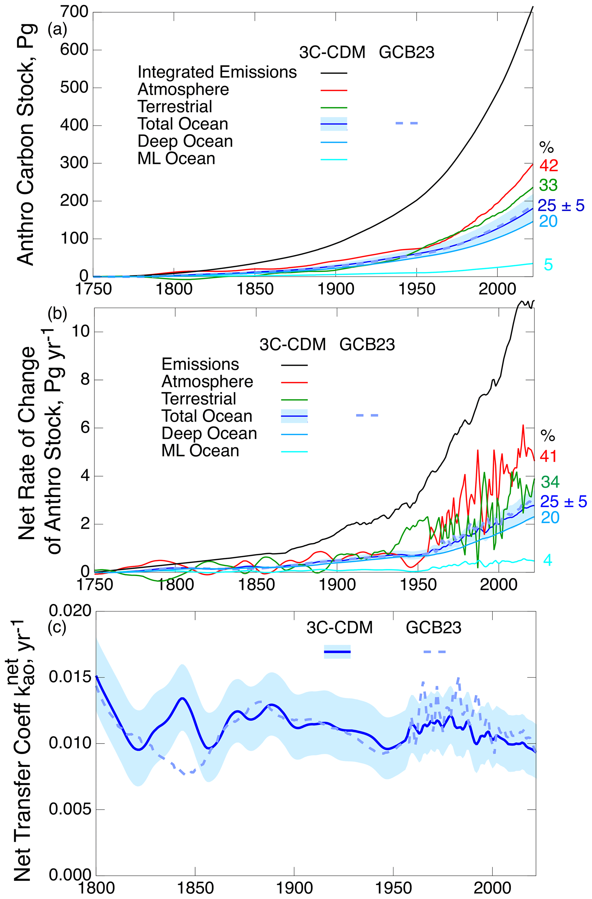
Figure 3 (a) Anthropogenic stocks of carbon in the several compartments of the biogeosphere from the 3C-CDM. (b) Rates of change of the several stocks. (c) Net transfer coefficient between the atmosphere and the total ocean compartment. Here and in subsequent figures, the dark blue curve denotes the central value as calculated by the 3C-CDM, and the shading denotes 1σ uncertainty in the modeled quantity based on the corresponding uncertainty in piston velocity v_p. The numbers on the right give the percentage of integrated emissions (a) or annual emissions (b) in the indicated compartments for the final year of the calculation, 2022. The dashed curves in all three panels show the values of the corresponding quantities from the GCB23 compilation for comparison purposes (Friedlingstein et al., 2023).

The second representation of the results is the rates of change of the several anthropogenic stocks (Fig. 3b), evaluated as the time derivatives of the corresponding stocks. The rate of change of the atmospheric stock, based on measurements and models, is taken from the historical tab of the data file accompanying the GCB23 report. As noted earlier, there is a slight natural flux of ∼ 0.6 Pg yr⁻¹ from the ocean to the atmosphere due to riverine flux into the ocean that must be accounted for in comparisons with observations. Neglecting this, the net flux from the atmosphere into the ocean is treated as anthropogenic. The net flux from the atmosphere to the ocean is equal to the rate of increase in the total ocean stock:

$$\begin{array}{}\text{(28)}& F_{\mathrm{ao}}^{\mathrm{net}}={\displaystyle \frac{\mathrm{d}{S}_{\mathrm{o}}}{\mathrm{d}t}}.\end{array}$$

The 1σ uncertainty range in the rate of increase in the ocean stock is calculated in the same manner as for the stock itself. For the total ocean, and also the TB (again, not modeled but calculated by difference), the rates of change represent the net flux from the atmosphere into the respective compartment; for the DO this rate of change is equal to the net flux from the ML to the DO. The numbers on the right represent the fraction of annual emissions taken up annually by the several compartments for the final year of the model run. Attention is called to the much greater fluctuations in the atmospheric stock subsequent to 1959 versus prior; this is a consequence of the use of measurements of S_a from CO₂ concentrations in air versus from ice cores prior to 1959, in which fluctuations are damped out in the data. The fluctuations are likewise enhanced in the stock in the total ocean and in the ML because of rather tight coupling of the ML to the atmosphere. In contrast, the stock in the DO remains rather smooth after the transition to using annual atmospheric data to drive the model; this is a consequence of the DO stock being (roughly) proportional to the integral of the ML stock, which damps fluctuations. The curves for the rates of change in the several stocks are roughly proportional to the stocks, with the constant of proportionality being the rate of change of atmospheric stock to the stock itself.

The third means of representing the results of this model (Fig. 3c) takes cognizance of the fact that while the stocks (Fig. 3a) in the several compartments and fluxes between the compartments are extensive properties of the system, the net transfer coefficients describing these fluxes (ratios of net fluxes to stocks of leaving compartments) are intensive properties of the system. Thus, it is useful to define, evaluate, and compare net transfer coefficients as a function of time within a given model or across models. As intensive properties, the net transfer coefficients are much more constant over the Anthropocene than the extensive properties, the stocks, or the fluxes because of the removal of the dependence on the secular growth of these quantities. Here, the net flux $F_{\mathrm{ao}}^{\mathrm{net}}$ (Fig. 3b) is in the direction of the atmosphere to the ocean. When the leaving compartment is the atmosphere, the net transfer coefficient from the atmosphere to the ocean is defined as

$$\begin{array}{}\text{(29)}& k_{\mathrm{ao}}^{\mathrm{net}}\equiv F_{\mathrm{ao}}^{\mathrm{net}}/S_{\mathrm{a}}^{\mathrm{ant}},\end{array}$$

shown as a function of time over the Anthropocene in Fig. 3c. The initial years of the model run are omitted from the figure as they are quite noisy because of the low values of the denominator quantity $S_{\mathrm{a}}^{\mathrm{ant}}\left(t\right)$ at small t. As anticipated, the net transfer coefficient exhibits much less secular change than either the stocks or the fluxes, allowing a more detailed examination of the time dependence. As seen below, this near constancy allows examination of the possible time dependence of $F_{\mathrm{ao}}^{\mathrm{net}}$.

The simple model described and presented here yields considerable insight. As an illustration, comparison of the net transfer coefficient for uptake of carbon by the DO $k_{\mathrm{md}}^{\mathrm{net}}$ obtained from the model results to the actual transport coefficient obtained from the piston velocity $k_{\mathrm{md}}=v_{\mathrm{p}}/z_{\mathrm{m}}$ (Fig. 4) illustrates the gradual decrease in $k_{\mathrm{md}}^{\mathrm{net}}$ from its initial value, equal to k_md, by about 12 % over the Anthropocene, which is a consequence of the return flux of anthropogenic carbon from the DO to the ML.

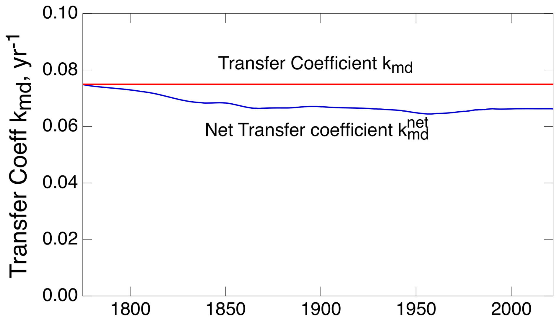
Figure 4 Transfer coefficient k_md and net transfer coefficient $k_{\mathrm{md}}^{\mathrm{net}}$ describing transport between the ML and the DO as a function of time over the Anthropocene.

Another important example is comparison of the gross anthropogenic fluxes between the atmosphere and the ML (Fig. 5a) and the gross and net anthropogenic fluxes between the ML and the DO (Fig. 5b). As shown in Fig. 5a, the return flux from the ML to the atmosphere is nearly equal to the forward flux from the atmosphere to the ML (7 % difference at the end of the run). Such near equality in gross fluxes is indicative of near equilibrium between the two compartments. In contrast, the difference in the gross fluxes between the ML and the DO is about an order of magnitude, and the gross flux between these compartments and the net flux, expressed as the fractional difference, is approximately 11 %. Thus, the rate-limiting step governing the overall net transfer from the atmosphere to the ocean is the transfer from the ML to the DO.

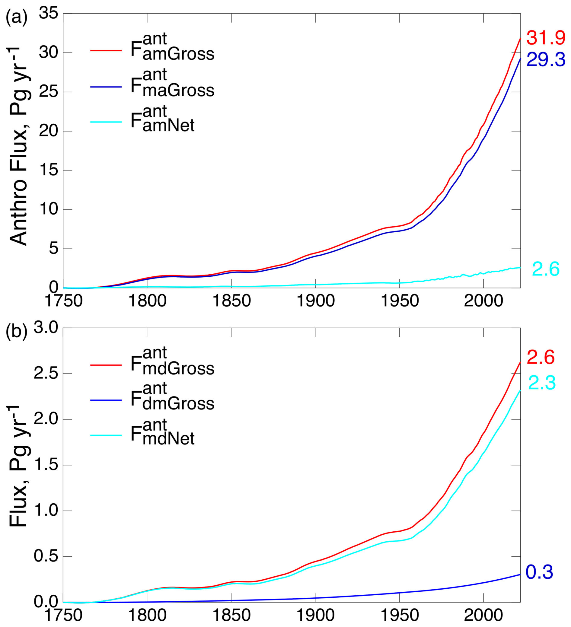
Figure 5 Gross and net anthropogenic fluxes (a) between the atmosphere and the ML and (b) between the ML and the DO over the Anthropocene, as calculated by the 3C-CDM. Numbers on the right give values for the year 2022.

The near equality of the forward and reverse fluxes between the atmosphere and the ML suggests that treating these two compartments as being in equilibrium would yield only slight differences in the evolution of the system. The pertinent calculation is readily carried out by integration of a single ODE, with the forcing that drives transfer from the ML to the DO being the stock in the ML, S_m, where S_m is assumed to be in equilibrium with the atmospheric stock, S_a. That is,

$$\begin{array}{}\text{(30)}& {\displaystyle \frac{\mathrm{d}{S}_{\mathrm{d}}^{\mathrm{ant}}}{\mathrm{d}t}}=k_{\mathrm{md}}{S}_{\mathrm{m}}^{\mathrm{ant}}-k_{\mathrm{dm}}{S}_{\mathrm{d}}^{\mathrm{ant}}\end{array}$$

for the initial condition $S_{\mathrm{d}}^{\mathrm{ant}}=\mathrm{0}$, where

$$\begin{array}{}\text{(31)}& \begin{array}{rl}{S}_{\mathrm{m}}^{\mathrm{ant}}\left(t\right)& =S_{\mathrm{m}}\left(t\right)-S_{\mathrm{m}}^{\mathrm{pi}}\mathrm{and}{S}_{\mathrm{m}}\left(t\right)=S_{\mathrm{m}}^{\mathrm{eq}}\left(t\right)\\ & =K_{\mathrm{am}}\left(S_{\mathrm{a}}\right)S_{\mathrm{a}}\left(t\right).\end{array}\end{array}$$

Treating the ML as being in equilibrium with the atmosphere and forcing the model by the ML stock reduce the model to a two-compartment model, namely 2C-CDM. Treating these compartments as being in equilibrium would afford the advantage of eliminating one model parameter, the deposition velocity k_am, thereby reducing the number of parameters in the model to one, the piston velocity v_p. This equilibrium assumption removes any dependence of the model results on the kinetics of CO₂ transfer between the atmosphere and the ML, also eliminating the need to represent the nonlinear relation between k_ma and k_am. Calculating the rate and extent of net transfer into the ML and the DO under this equilibrium assumption lends strong support to the near-equilibrium hypothesis, with the differences in the stocks of the two compartments – between the full kinetic treatment and the treatment under the assumption between the atmosphere and ML – at the end of the model run being slight, amounting to only 7 % or 8 % (Fig. 6).

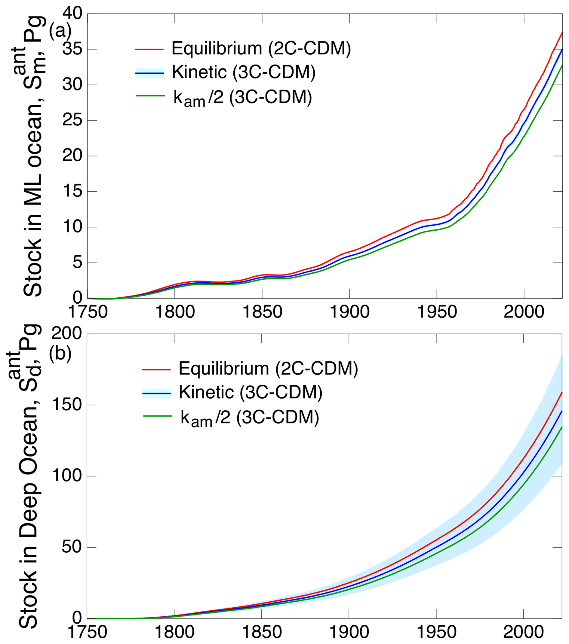
Figure 6 Time dependence of anthropogenic stocks (a) in the ML and (b) in the DO, as calculated with the 3C-CDM (denoted “kinetic”, transfer coefficient k_am= 0.119 yr⁻¹), with k_am decreased by a factor of 2 and with a model variant 2C-CDM that treats the stocks in the atmosphere and the ML as being in equilibrium. Shading denotes 1σ uncertainty based on the corresponding uncertainty in piston velocity v_p; the shaded band in a is barely visible.

The sensitivity of uptake into the ML and the DO to the value of k_am was further examined by reducing the value of this transfer coefficient by a factor of 2, also shown in Fig. 6. Figure 6a shows that the anthropogenic stock in the ML depends only weakly on k_am (−7 % at the end of the model run for k_am divided by 2 or +7 % for the equilibrium state, equivalent to k_am=∞); this insensitivity is a further demonstration of near equilibrium between the two compartments. The anthropogenic ML stock is wholly insensitive to the value of the piston velocity v_p, with the range of that uncertainty propagated into the uncertainty in the ML stock (∼ 25 %) – yet a further consequence of the stock in the ML being in near equilibrium with the atmosphere. In contrast, the extent of uptake into the DO (Fig. 6b) is controlled only by the piston velocity, which governs the rate of transfer from the ML to the DO.

Comparing the results obtained with the equilibrium model versus the full kinetic model with the propagated uncertainty due to uncertainty in v_p (Fig. 7a) shows that the difference in total anthropogenic ocean stock, taken as the sum of the anthropogenic stocks in the ML and DO, between the equilibrium model and the kinetic model (9 % at the end of the model run) is well less than the propagated uncertainty in this quantity due to uncertainty in v_p, shown by the shaded regions surrounding the respective central values (about ± 20 %). This finding also holds true (Fig. 7b) for the net atmosphere–ocean flux and (Fig. 7c) for the intensive quantity, the net transfer coefficient from the atmosphere to the total ocean $k_{\mathrm{ao}}^{\mathrm{net}}$ (Eq. 29). As the differences between the quantities for the kinetic model and the equilibrium model are well within the uncertainty range due to uncertainty in v_p, the equilibrium model might be used with confidence for most practical purposes. However, for completeness, here the results from the kinetic model are compared to the results of other models in Sect. 6. Shown also in the several panels of Fig. 7 are the results from the kinetic model with the transfer coefficient k_am diminished by a factor of 2, which are all well within the propagated uncertainty from uncertainty in v_p, further illustrating the rather small uncertainty in the several measures of the extent and rate of uptake of CO₂ into the global ocean due to uncertainty in k_am.

Also shown in Fig. 7c is the ratio of the anthropogenic stock in the ML to that in the atmosphere, for both the equilibrium model and the two kinetic models. As expected, this ratio is less for the kinetic models than for the equilibrium model. Importantly, the solubility curves exhibit a gradual but clear decrease over the years 1800–2022, amounting to 17 % for the equilibrium model. Because of fluctuations in the net transfer coefficient, the decrease in solubility is more readily discernable than the decrease in the transfer coefficients. Plotting the quantities proportionally on the same graph highlights the decrease in the net transfer coefficient, the pertinent intensive measure of the uptake of the anthropogenic CO₂ rate over the industrial period. Comparison of the curves for $k_{\mathrm{ao}}^{\mathrm{net}}$ and $S_{\mathrm{m}}^{\mathrm{ant}}/S_{\mathrm{a}}^{\mathrm{ant}}$ suggests that $k_{\mathrm{ao}}^{\mathrm{net}}$ may likewise have decreased by a similar amount over the 1800–2022 period, with the decrease perhaps being the greatest and most evident subsequent to about 1960. The return flux from the DO to the ML (Fig. 4) would also contribute to a decrease in $k_{\mathrm{ao}}^{\mathrm{net}}$. Plotting the net uptake rate as the intensive quantity $k_{\mathrm{ao}}^{\mathrm{net}}$ (Fig. 7c) rather than as the extensive quantity, the net flux $F_{\mathrm{ao}}^{\mathrm{net}}$, as has been customary, makes it possible to discern any slight decrease in the net uptake rate due to decrease in equilibrium solubility, the effect of which is swamped in $F_{\mathrm{ao}}^{\mathrm{net}}$ by the increase in net flux due to an increase in the atmospheric stock.

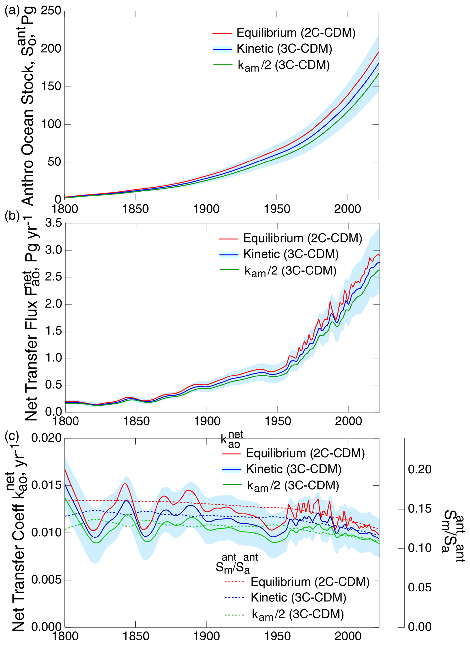
Figure 7 Time dependence of (a) anthropogenic stock in the global ocean, (b) the net atmosphere–ocean flux, and (c) the net atmosphere–ocean transfer coefficient $k_{\mathrm{ao}}^{\mathrm{net}}$ (left-hand axis), as calculated with the 3C-CDM, which explicitly represents the kinetics of mass transport between the atmosphere and the ML with a model variant, the 2C-CDM, which treats the stocks in those two phases as being in equilibrium, and with k_am artificially diminished by a factor of 2 in the 3C-CDM. Dashed curves in (c), with values shown by the auxiliary right-hand axis, proportional to the left-hand axis, denote the ratio of anthropogenic stock in the ML to that in the atmosphere in the three model variants.

Although in the 3C-CDM the stock growth rate of anthropogenic carbon in the TB and transfer coefficient from the atmosphere to the TB are determined by difference, the stock and growth rate in the sum of the ocean and TB compartments and corresponding transfer coefficient from the atmosphere to these two compartments are determined entirely by observations:

$$\begin{array}{}\text{(32)}& S_{\mathrm{ot}}^{\mathrm{ant}}\equiv S_{\mathrm{o}}^{\mathrm{ant}}+S_{\mathrm{t}}^{\mathrm{ant}}=\int Q_{\mathrm{ant}}\mathrm{d}t-S_{\mathrm{a}}^{\mathrm{ant}}.\end{array}$$

The net transfer flux is determined similarly,

$$\begin{array}{}\text{(33)}& {\displaystyle \frac{\mathrm{d}{S}_{\mathrm{ot}}^{\mathrm{ant}}}{\mathrm{d}t}}=Q_{\mathrm{ant}}-{\displaystyle \frac{\mathrm{d}{S}_{\mathrm{a}}^{\mathrm{ant}}}{\mathrm{d}t}},\end{array}$$

as is the net transfer coefficient:

$$\begin{array}{}\text{(34)}& k_{\mathrm{a}\to \mathrm{o}+\mathrm{t}}^{\mathrm{net}}={\displaystyle \frac{Q_{\mathrm{ant}}-\frac{\mathrm{d}{S}_{\mathrm{a}}^{\mathrm{ant}}}{\mathrm{d}t}}{S_{\mathrm{a}}^{\mathrm{ant}}}}.\end{array}$$

Here, the anthropogenic emissions $Q_{\mathrm{ant}}=Q_{\mathrm{ff}}+Q_{\mathrm{lu}}$ are used for the first time in this analysis. Because of uncertainty in this quantity, the value of $k_{\mathrm{a}\to \mathrm{o}+\mathrm{t}}^{\mathrm{net}}$ must be regarded with caution. Nonetheless, examination of the three net transfer coefficients, $k_{\mathrm{a}\to \mathrm{o}+\mathrm{t}}^{\mathrm{net}}$, $k_{\mathrm{at}}^{\mathrm{net}}$, and $k_{\mathrm{ao}}^{\mathrm{net}}$, is informative (Fig. 8); here, $k_{\mathrm{at}}^{\mathrm{net}}$ and $k_{\mathrm{ao}}^{\mathrm{net}}$ are shown for v_p= 7.5 m yr⁻¹ and k_am= 0.119 yr⁻¹. The net transfer coefficient $k_{\mathrm{ao}}^{\mathrm{net}}$, as calculated with the 3C-CDM, is as shown in Fig. 7c. Variation in $k_{\mathrm{ao}}^{\mathrm{net}}$ is dwarfed by that in $k_{\mathrm{a}\to \mathrm{o}+\mathrm{t}}^{\mathrm{net}}$ and $k_{\mathrm{at}}^{\mathrm{net}}$. As noted, $k_{\mathrm{a}\to \mathrm{o}+\mathrm{t}}^{\mathrm{net}}$ is independent of the model calculations, and $k_{\mathrm{at}}^{\mathrm{net}}$ is only weakly dependent on the model calculations through subtraction of the fairly constant (on the scale of Fig. 8) value of $k_{\mathrm{ao}}^{\mathrm{net}}$. On the timescale of the figure, 1850–2022, none of the quantities exhibits appreciable time dependence. As noted in conjunction with Fig. 7c, there may be a slight decrease over the time period that might be discerned in comparison with the ratio of the equilibrium stocks in the atmosphere and the ocean. The large fluctuations in $k_{\mathrm{a}\to \mathrm{o}+\mathrm{t}}^{\mathrm{net}}$ and $k_{\mathrm{at}}^{\mathrm{net}}$ in the earlier years of the record may be due in large part to fluctuations in Q_ant, amplified by small values of $S_{\mathrm{a}}^{\mathrm{ant}}$ in the denominator of Eq. (34). Raupach et al. (2014) called attention to the appreciable decrease in $k_{\mathrm{a}\to \mathrm{o}+\mathrm{t}}^{\mathrm{net}}$ for time subsequent to 1959. The slopes of the least-squares fits to $k_{\mathrm{a}\to \mathrm{o}+\mathrm{t}}^{\mathrm{net}}$ and $k_{\mathrm{at}}^{\mathrm{net}}$ over this period are essentially identical to each other and several-fold greater than the slope of $k_{\mathrm{ao}}^{\mathrm{net}}$, suggesting that any decrease in the net removal rate of excess CO₂ from the atmosphere over this period would be dominated by a decrease in the net uptake rate into the TB. However, the large fluctuations in these quantities in the earlier years of the record might raise questions regarding the confidence that can be placed in that inferred decrease.

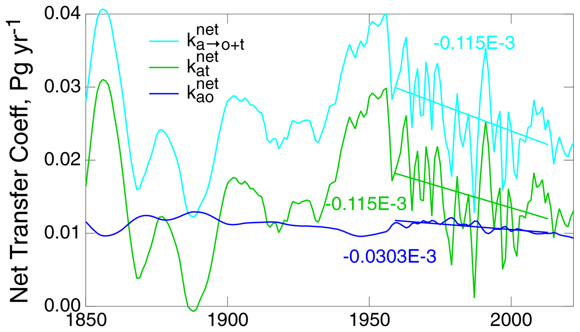
Figure 8 Time dependence of the net transfer coefficients from the atmosphere to the global ocean and terrestrial biosphere taken together, $k_{\mathrm{a}\to \mathrm{o}+\mathrm{t}}^{\mathrm{net}}$, as determined from observations; to the global ocean, $k_{\mathrm{ao}}^{\mathrm{net}}$, as determined by the 3C-CDM; and their difference, $k_{\mathrm{at}}^{\mathrm{net}}$. Also shown are least-squares fits to the three quantities over the time period 1959–2022 and their slopes in units of Pg yr⁻¹ yr⁻¹.

Radiocarbon

Examination of the stocks of radiocarbon in the two ocean compartments (and their sum) and comparison with models and observations provide additional assessment of the skill of the present (or any) model, especially as the stock of atmospheric ¹⁴CO₂ exhibited a very different time history compared to ordinary CO₂, as a consequence of the pulse in concentration due to atmospheric weapons testing (generally denoted “bomb carbon”) and its rapid decline subsequent to cessation of these tests in 1963. The concentration-driven model's treatment of radiocarbon is similar to that for ordinary carbon. However, as the amount of radiocarbon that is transferred between the atmosphere and the ML is so slight that it does not perturb the DIC equilibrium, the simple (DIC-dependent) equilibrium constant between the two phases is used. The rate of transfer from the atmosphere to the ML is the same as for ordinary carbon (Eq. 22); kinetic and equilibrium isotope effects are small and hence neglected. For the stocks of radiocarbon denoted R and the fluxes denoted G, the gross flux of ¹⁴CO₂ from the atmosphere to the ML is

$$\begin{array}{}\text{(35)}& G_{\mathrm{am}}=k_{\mathrm{am}}{R}_{\mathrm{a}},\end{array}$$

and the gross flux from the ML to the atmosphere is

$$\begin{array}{}\text{(36)}& G_{\mathrm{ma}}=k_{\mathrm{ma}}{R}_{\mathrm{m}}.\end{array}$$

Here,

$$\begin{array}{}\text{(37)}& k_{\mathrm{ma}}={\displaystyle \frac{k_{\mathrm{am}}}{K_{\mathrm{am}}}}\end{array}$$

and

$$\begin{array}{}\text{(38)}& K_{\mathrm{am}}={\left({\displaystyle \frac{S_{\mathrm{m}}}{S_{\mathrm{a}}}}\right)}_{\mathrm{eq}}.\end{array}$$

The corresponding differential equations are

$$\begin{array}{}\text{(39)}& \begin{array}{rl}& {\displaystyle \frac{\mathrm{d}{R}_{\mathrm{m}}^{\mathrm{ant}}}{\mathrm{d}t}}=k_{\mathrm{am}}{R}_{\mathrm{a}}^{\mathrm{ant}}-k_{\mathrm{am}}{K}_{\mathrm{ma}}{R}_{\mathrm{m}}^{\mathrm{ant}}-k_{\mathrm{md}}{R}_{\mathrm{m}}^{\mathrm{ant}}+k_{\mathrm{dm}}{R}_{\mathrm{d}}^{\mathrm{ant}}\\ & {\displaystyle \frac{\mathrm{d}{R}_{\mathrm{d}}^{\mathrm{ant}}}{\mathrm{d}t}}=k_{\mathrm{md}}{R}_{\mathrm{m}}^{\mathrm{ant}}-k_{\mathrm{dm}}{R}_{\mathrm{d}}^{\mathrm{ant}}.\end{array}\end{array}$$

The differential equations are analogous to Eq. (27) but with the differential equilibrium constant $K{{}^{\prime }}_{\mathrm{ma}}$ replaced by the ordinary equilibrium constant K_ma, which is an order of magnitude greater (Appendix A, Fig. A1), and the first equation being in the stock itself rather than in the departure from equilibrium. The initial condition is that all the anthropogenic stocks are zero in the year 1750. The equations are linear with constant coefficients, except for the dependence of K_am on time due to the decrease in CO₂ solubility over the industrial period (∼ 45 %, Fig. A1). As with the calculations for CO₂, the anthropogenic stock of ¹⁴C in the terrestrial biosphere is evaluated as the difference between integrated emissions and the increases in the stocks in the atmosphere and the ocean.

The results of the model calculation are shown in Fig. 9; here the several quantities are presented in units of 1×10²⁶ atoms in the global atmosphere (also shown for reference are integrated emissions, which are not used in the calculations). The atmospheric stock that drives the calculation is from the following measurements: Stuiver et al. (1998), the tabulations of Graven et al. (2017), and Hua et al. (2022). Most notable is the strong increase in anthropogenic atmospheric emissions due to bomb carbon over the years 1950–1963 and resultant increases in the stocks in the other compartments. This was then followed by an abrupt decrease in emissions, resulting from the ban on atmospheric testing of nuclear weapons that took effect in late 1963 and the resultant more gradual decrease in atmospheric ¹⁴CO₂ stock.

Prior to 1950 the atmospheric stock increased gradually. This increase in stock is opposite in sign to the well-known decrease in the isotopic ratio, Δ¹⁴CO₂, which is a different way of expressing the same measurements and which is the hallmark of the Suess effect (Suess, 1955) that served as an early demonstration of the increase in atmospheric CO₂ due to emissions of fossil fuel CO₂. The increase in atmospheric stock of ¹⁴CO₂ over this period is a consequence of the increase in the stock of cold CO₂ from fossil fuel emissions outweighing the decrease in Δ¹⁴CO₂ (Schwartz et al., 2024).

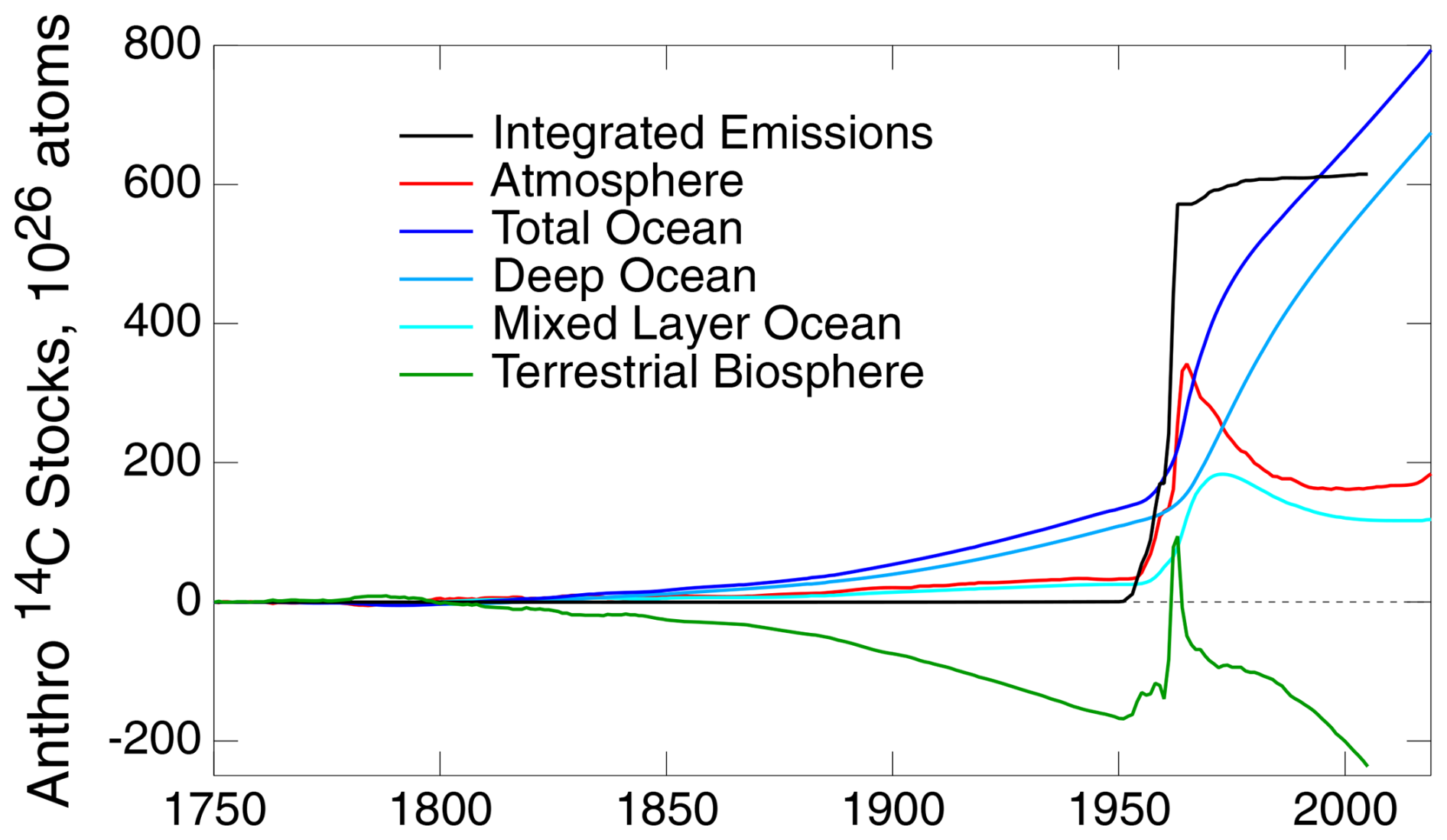
Figure 9 Anthropogenic stocks of radiocarbon in the several compartments of the biogeosphere as calculated with the 3C-CDM. Atmospheric stock is calculated from measurements (Stuiver et al., 1998; Graven et al., 2017; Hua et al., 2022). Emissions prior to 1950 are taken as zero; emissions data for the years 1951–2005 were provided by Tobias Naegler (personal communication, 2020), based on the Yang et al. (2000) emissions inventory.

Over the pre-bomb period, the stocks of ¹⁴C in the two ocean compartments increased in response to the increase in atmospheric stock. As the anthropogenic stock in the DO is the integral of net transfer from the ML, essentially all from the ML to the DO, this stock increases continuously over the entire time period and is the major contributor to the total anthropogenic ocean stock. The sum of the increases in the three compartments substantially exceeds the anthropogenic emissions over this period, which are essentially zero. The question arises: where is this ¹⁴C coming from? The only possible source is the terrestrial biosphere, for which the change in stock, evaluated as the difference between emissions (essentially zero) and the increases in the stocks in the atmosphere and ocean, is negative throughout this period. This, in turn, prompts a second question: why is the stock of ¹⁴C in the TB decreasing? At preindustrial time, prior to significant emissions of cold CO₂ from fossil fuel combustion, the system was in isotopic equilibrium, that is, equal and opposite fluxes of both cold and hot CO₂ between the atmosphere and the TB. As Δ¹⁴C of atmospheric CO₂ decreased because of the input of cold CO₂ into the atmosphere, the tendency toward isotopic equilibrium required a decrease in Δ¹⁴C of carbon in the TB, which could be achieved only by net transfer of Δ¹⁴C from the TB to the atmosphere, leading to the decrease in hot C in the TB and the increase in hot CO₂ in the atmosphere, as shown in measurements (Schwartz et al., 2024) and in more detail in the open discussion of the present paper (https://egusphere.copernicus.org/preprints/2024/egusphere-2024-2893/#AC4, last access: 2 June 2025). All of this is captured by the 3C-CDM, as shown in Fig. 9.

6 Comparison with other models and with observations

Results obtained with the 3C-CDM, specifically the anthropogenic increase in the ocean stock, the time derivative of this increase, and the associated net transfer coefficient, are compared here with the corresponding quantities from other models. These models include concentration-driven and emissions-driven models. The 3C-CDM calculates the stocks in the two ocean compartments, with a key finding being that the majority (∼ 80 %) of the ocean uptake of anthropogenic carbon over the Anthropocene is into the DO compartment with only a minor fraction (∼ 20 %) into the ML (Fig. 3a), and thus that the uptake into the total ocean is governed mainly by k_md. Most models against which the 3C-CDM is compared provide only net uptake of anthropogenic carbon from the atmosphere into the total ocean. Hence, it is the sum of the anthropogenic stocks in the ML and the DO and the net anthropogenic flux from the atmosphere into the ML (which is the sum of the rate of change of the stocks in the two compartments) that can be compared across models here.

As an initial comparison, Fig. 10 shows a compilation (Wang et al., 2016) of net atmosphere–ocean flux over the 1881–2005 period from 13 carbon cycle models that participated in the Coupled Model Intercomparison Project Phase 5 (CMIP5) of the World Climate Research Programme, together with the net atmosphere–ocean flux from the 3C-CDM, as shown in Fig. 3b. The CMIP5 models were emissions driven rather than concentration driven, as in the 3C-CDM. The net uptake flux calculated with the 3C-CDM closely matches the center of gravity of the net flux of the CMIP5 models (after upward adjustment of those fluxes by 0.3 Pg yr⁻¹ to account for preindustrial riverine flow), all increasing from roughly 0.2 Pg yr⁻¹ in the year 1881 to approximately 2.3 Pg yr⁻¹ in the year 2005. However, the spread of the fluxes of the CMIP5 models (among the set of models and as characterized by the large fluctuations in the results of individual models) substantially exceeds the 1σ uncertainty associated with the 3C-CDM results throughout most of the modeled period, up until about 2005, by which time the uncertainty in the 3C-CDM results, which scales in proportion to the net flux, becomes comparable to the intermodel spread of the CMIP5 models. This situation suggests that the atmosphere–ocean flux calculated with the 3C-CDM is comparable to that of the individual CMIP5 models, albeit without the large sub-decadal fluctuations exhibited by most of those models.

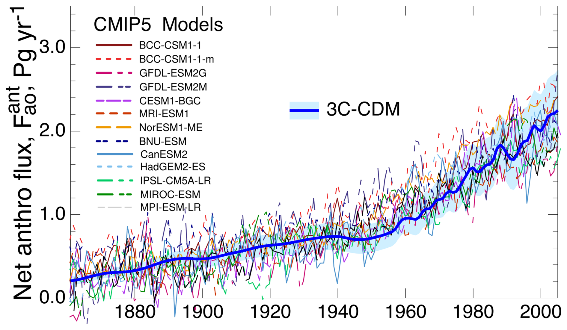
Figure 10 Comparison of net uptake flux, as in Fig. 7b, of anthropogenic atmospheric CO₂ into the global ocean, as determined with the 3C-CDM, with that calculated by several models participating in the CMIP5 intercomparison. CMIP5 data are given as compiled by Wang et al. (2016, their Fig. 1), augmented by 0.3 Pg yr⁻¹ to account for preindustrial natural flux.

The results obtained with the 3C-CDM were compared in Fig. 3 with several measures of the net ocean uptake of excess atmospheric CO₂, as reported regularly by the GCB project by Friedlingstein et al. (2023). The quantity denoted here as net atmosphere–ocean flux is denoted “ocean sink” by Friedlingstein et al. (2023), although this cannot be considered a true, irreversible sink because of return flux from the DO to the ML that would diminish net ocean uptake. This quantity, which is reported in the historical tab of the data tables that accompanied the 2023 Global Carbon Budget (GCB23; Friedlingstein et al., 2023), is a synthesis of multiple model and observational results. The central values of the several measures of the net uptake of excess CO₂ by the global ocean obtained with the 3C-CDM – the anthropogenic ocean stock (Fig. 3a), the net flux (Fig. 3b), and the net transfer coefficient (Fig. 3c) – are essentially identical, within the uncertainty associated with the 3C-CDM results, to the results presented by the GCB23 budget.

As noted above, the intensive quantity, the net transfer coefficient (Fig. 7c), is capable of yielding a much more sensitive comparison than can be obtained with either the anthropogenic stock (Fig. 7a) or the rate of increase in that stock (equivalent to net atmosphere–ocean flux; Fig. 7b), both of which are extensive quantities. For that reason, much of the following comparison is on the net transfer coefficient from the atmosphere to the ocean, $k_{\mathrm{ao}}^{\mathrm{net}}$, defined and evaluated by Eq. (29).

The results of the 3C-CDM are now compared in more detail with the data presented by GCB23. For the period prior to 1959, at which time there was a change in the methodology of the calculation of the sink rate given by GCB23, the ocean sink rate reported by GCB23 was the average of two data sets, that of DeVries (2014) and that of Khatiwala et al. (2013). Briefly, DeVries (2014) determined the net atmosphere–ocean transfer flux by means of the steady-state global Ocean Circulation Inverse Model (OCIM), constrained by momentum balance and the continuity equation, taking into account the frictional, Coriolis, and barotropic pressure forces and the imposed surface wind stress and baroclinic pressure forces. The model is discretized on a grid with 2° horizontal resolution and 24 unevenly spaced vertical levels in the ocean with thickness ranging from 30 m at the surface to 500 m at depth. The parameters of the model are constrained by global observations of potential temperature, salinity, radiocarbon, and CFC-11; these tracers were assimilated into the model to obtain optimal estimates of the climatological mean (steady-state) ocean circulation, ventilation, and air–sea gas exchange rates. The optimized circulation and air–sea gas exchange rates from this model were then used to simulate the oceanic uptake of anthropogenic CO₂ over the industrial era, with the amount of anthropogenic CO₂ estimated as the difference between a time-varying run, in which surface DIC concentration, in equilibrium with global and annual mean atmospheric CO₂, was increased according to observations, and a simulation in which it was held constant. The DeVries time series data are available from the cited paper.

Khatiwala et al. (2013) presented a synthesis of observational and model-based estimates of the storage and transport of anthropogenic DIC in the global ocean, obtained by three approaches: (1) an examination of the perturbation to the carbonate equilibrium, (2) Green's function method representing tracer transport, and (3) a transit time distribution method. These three approaches yielded the anthropogenic inventory for the year 1994 of 106 ± 17, 108 ± 14, and 114 ± 22 Pg, respectively, with the best estimate for the year 2010 of 155 ± 31 Pg. No time series was presented for the Khatiwala data; however it was possible to infer the time series from the GCB average of the two time series and the DeVries time series.

The three time series are shown in Fig. 11 as the net atmosphere–ocean transfer coefficient $k_{\mathrm{ao}}^{\mathrm{net}}$. Also shown in the figure is the net transfer coefficient obtained with the 3C-CDM, together with its associated uncertainty, as in Fig. 3c. The comparison of the net transfer coefficient with the two time series and their average shows that the 3C-CDM results rather closely match those of all three time series. From about 1860–1959, the values of $k_{\mathrm{ao}}^{\mathrm{net}}$ obtained with the 3C-CDM agree with the two data sets and their average, well within the uncertainty range of the 3C-CDM due to 1σ uncertainty in v_p.

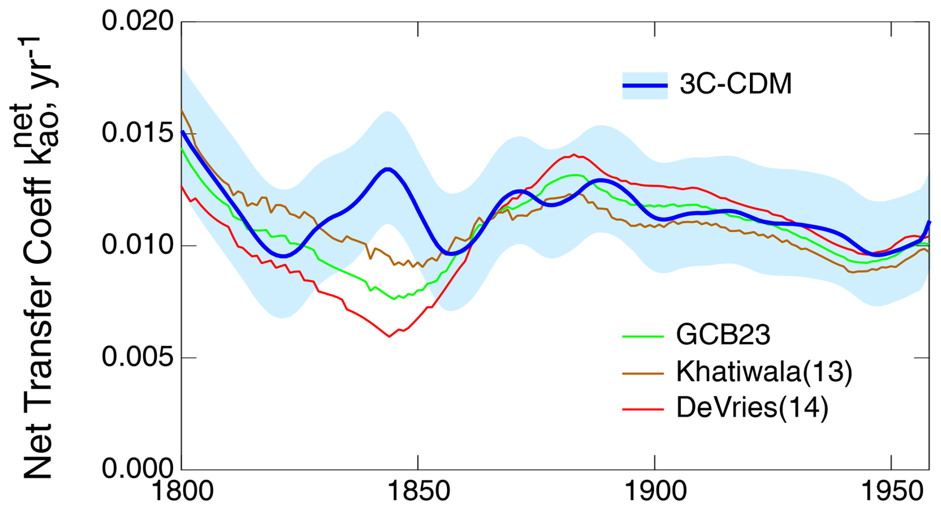
Figure 11 Time dependence of the net transfer coefficient from the atmosphere to the global ocean ($k_{\mathrm{ao}}^{\mathrm{net}}$) over the 1800–1958 period, as given by the GCB23 project (data tables accompanying Friedlingstein et al., 2023, historical tab), DeVries (2014), and Khatiwala et al. (2013, as inferred from the GCB average and the DeVries, 2014, data set).

For the time period subsequent to the year 1959, GCB23 presented global and annual mean net atmosphere to ocean flux as an average from two sets of data, both of which can be considered concentration driven. The first set consisted of what GCB23 denoted as “observation-based fCO₂ products” for eight regression models, where f denotes the fugacity of CO₂, for all practical purposes equivalent to the stock used here to drive the 3C-CDM. The second set consisted of 10 global ocean biogeochemistry models (GOBMs). The approaches taken in those studies are briefly summarized here, and the results of the individual model runs are presented here as the global and annual mean net atmosphere–ocean transfer coefficient, evaluated using Eq. (29) from the net fluxes presented by GCB23 and the global and annual mean anthropogenic stock in the atmosphere, also presented by GCB23. These results are then compared to the results obtained with the 3C-CDM.

For the fCO₂ study, the spatial resolution of most regression models was 1°×1° (with one model having a resolution of 2°×2.5°); the temporal resolution for most models was monthly. The carbon dioxide concentration for the different models was obtained from a variety of time- and space-dependent data sets regridded to the model resolution by inversion methods, such as multi-dimensional regressions, neural networks, and machine learning. Further information on the methods employed by the several models is presented in Table S3 of the Supplement of GCB23. Here, in calculating the global mean net transfer coefficient using Eq. (29), the global mean anthropogenic atmosphere–ocean flux data were used as provided in the ocean sink tab of the GCB23 data set; these data are explicitly meant to be anthropogenic fluxes (i.e., not including the riverine flux), so the data may be directly compared to the anthropogenic fluxes calculated with the 3C-CDM. The results are shown in Fig. 12a as time series along with the results of the 3C-CDM. The net transfer coefficient calculated with the 3C-CDM agrees rather closely with the results of most of the models calculating net atmosphere–ocean flux according to the fCO₂ protocol, with the spread among the models comparable to the uncertainty range of the 3C-CDM.

Also shown in Fig. 12a is the time series of $k_{\mathrm{ao}}^{\mathrm{net}}$ calculated from flux data presented by McKinley et al. (2020) for a diagnostic box model consisting of single compartments for the atmosphere, ML, and DO, similar to the present model, forced with the observed atmospheric CO₂ mixing ratio, using what those investigators characterized as “reasonable” default parameter choices z_m of 200 m and an ocean overturning circulation rate of 60 Sv, corresponding to a k_md of 0.262 yr⁻¹. The model was also forced by surface ocean temperature changes due to eruptions of three large volcanoes during this period (Agung 1963, El Chichón 1982, and Pinatubo 1991). The time series of $k_{\mathrm{ao}}^{\mathrm{net}}$ of this model agrees closely with the other models shown and with the present model. Here it can be observed that in this model the piston velocity v_p was not constrained by observations and that the same net air–sea flux could be obtained with a range value pairs of v_p and z_m, a lower value of v_p being compensated for by a greater value of z_m and vice versa.

The 10 models participating in the GOBM study simulated both the natural and the anthropogenic CO₂ cycles in the ocean. The increase in ocean DIC stock was evaluated as the difference, after correction for model drift, between ocean stock calculated with historical atmospheric CO₂ increase and what GCB23 (Supplement, Section S.3.2) denoted as normal-year climate minus that with constant atmospheric CO₂ and normal-year climate forcing. The horizontal resolution of the models was lower than 1 to 2° depending on the model; the number of vertical levels in the ocean in the several models ranged from 31 to 75. Atmospheric CO₂ forcing was mainly as provided by the GCB, with annual or monthly resolution, and in some instances with partial pressure adjusted by local total pressure. Further information is provided in Table S2 of the Supplement of GCB23. Again in calculating the global mean net transfer coefficient here, the global mean atmosphere–ocean flux data were used as provided in the ocean sink tab of the GCB23 data set. The results are shown in Fig. 12b, again with the results of the 3C-CDM. Again, the atmosphere–ocean flux calculated with the 3C-CDM agrees closely with the results of most of the models, with the uncertainty range of the 3C-CDM, about ± 20 %, essentially overlapping the data reported by the several models contributing to the GOBM protocol.

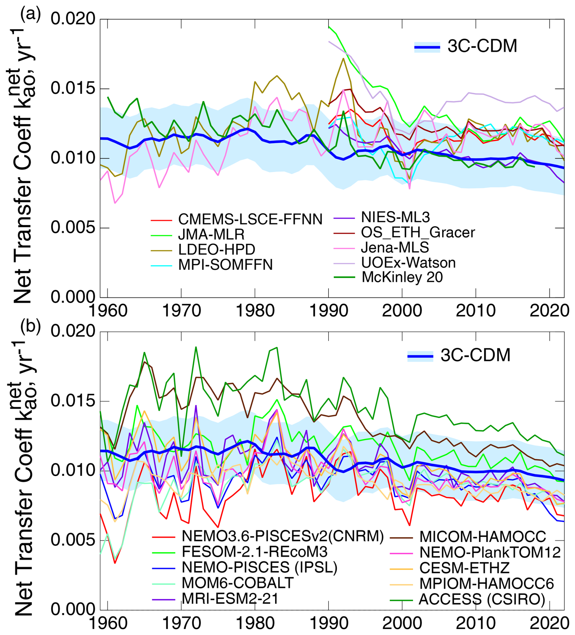
Figure 12 (a) Time dependence of the net transfer coefficient from the atmosphere to the global ocean, as calculated from net atmosphere–ocean fluxes for eight observation-derived data sets (fCO₂) presented by the GCB23 (the data from the UoEx-Watson model, although flagged by the GBC23, are shown for completeness), together with $k_{\mathrm{ao}}^{\mathrm{net}}$, as calculated by the 3C-CDM. Also shown is the net transfer coefficient calculated from flux data for the three-compartment, concentration-driven model of McKinley et al. (2020), as described in the text. Panel (b) is the same as panel (a) but for 10 concentration-driven global ocean biochemistry models calculated according to the GOBM protocol of the GCB23 project. For references to the fCO₂ and GOBM models, see Friedlingstein et al. (2023).

A further set of modeling data against which to compare the results of the 3C-CDM was presented by Melnikova et al. (2023), who compared net atmosphere–ocean fluxes calculated from concentration-driven model runs using two different types of models: Earth system models (ESMs) and what they refer to as simple climate models (SCMs), with the latter having roughly four ocean and four land compartments, depending on the model. In their study, Melnikova et al. (2023) made use of the results of the Reduced Complexity Model Intercomparison Project (RCMIP; Nicholls et al., 2020, 2021). For a brief description of the models examined and for references to the models, see Melnikova et al. (2023). For each of the models, the net transfer coefficient $k_{\mathrm{ao}}^{\mathrm{net}}$ was calculated using Eq. (29) through the ocean uptake rates and the atmospheric CO₂ mixing ratios compiled by Melnikova et al. (2023) (I thank Irina Melnikova for making the data developed in their study available; the data are available at https://zenodo.org/records/10162686/files/SSP2.xlsx?download=1, last access: 29 August 2024). In calculating $k_{\mathrm{ao}}^{\mathrm{net}}$, the values of S_a for the individual models were used if presented; otherwise the values specified in the RCMIP were employed. The resulting time series are shown in Fig. 13 together with the results from the 3C-CDM. The values of $k_{\mathrm{ao}}^{\mathrm{net}}$ for the ESMs and several of the SCMs exhibited large fluctuations in the early years of the intercomparison runs; the fluctuations were even greater in the time period extending back to 1850, the first year for which the data are available, presumably indicative of transients associated with initializations of some components of the models. However, by the end of the time series, the values of $k_{\mathrm{ao}}^{\mathrm{net}}$ for all the models fall within the 1σ uncertainty range of the 3C-CDM results, which is roughly 0.01 ± 0.002 yr⁻¹ in the year 2022.

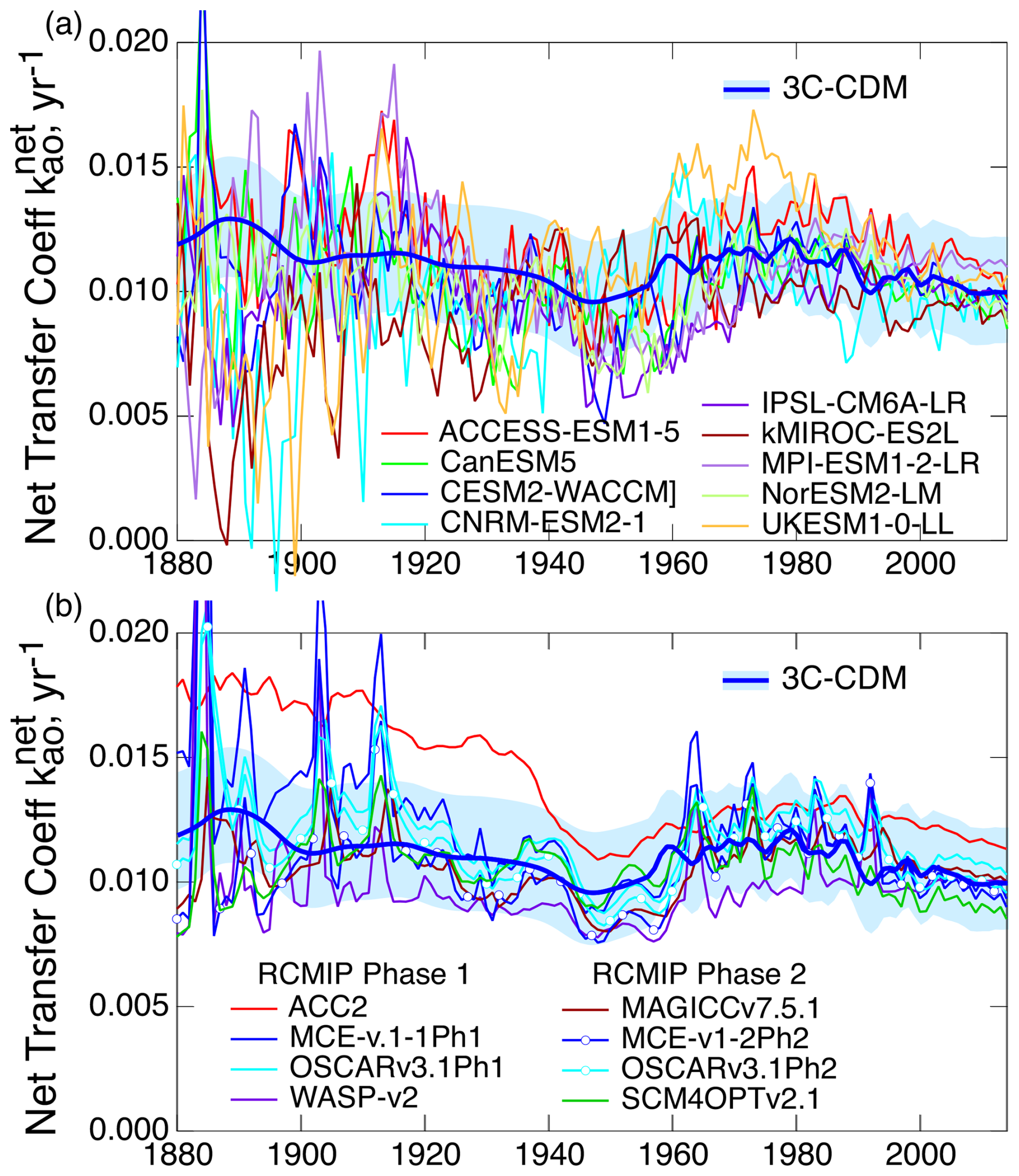
Figure 13 Time dependence of the net transfer coefficient from the atmosphere to the global ocean, as calculated from net atmosphere–ocean fluxes in concentration-driven runs by (a) nine Earth system models and (b) eight simple climate models. Values of $k_{\mathrm{ao}}^{\mathrm{net}}$ were calculated from net atmosphere–ocean fluxes determined in the several studies as compiled by Melnikova et al. (2023). Also shown are results from the 3C-CDM. Instances of the same model being employed in the two phases of the RCMIP are distinguished by markers on the curves.

While models are plentiful, measurements are sparse, requiring sufficient samples as a function of location and depth to allow evaluation of a global integral, which in turn requires a sustained effort to conduct soundings along a sufficient number of transects to allow interpolation, and with the further requirement that the measurements must be sufficiently accurate to quantify the small anthropogenic increment in DIC against the much larger total DIC concentration. A fair assessment of the status of measurement-based assessment of global stock of ocean DIC is that of DeVries (2022), shown by the markers in Fig. 14. Based on that standard, the 3C-CDM accurately reproduces the measurements. That is probably the most that can be said about the accuracy, based on direct measurement of incremental DIC concentration, of the 3C-CDM or any model used to calculate total ocean DIC. Also shown in the figure is the stock of ocean DIC calculated using the Ocean Circulation Inverse Model developed by DeVries and colleagues (DeVries, 2022) which also accurately represents the measurements.

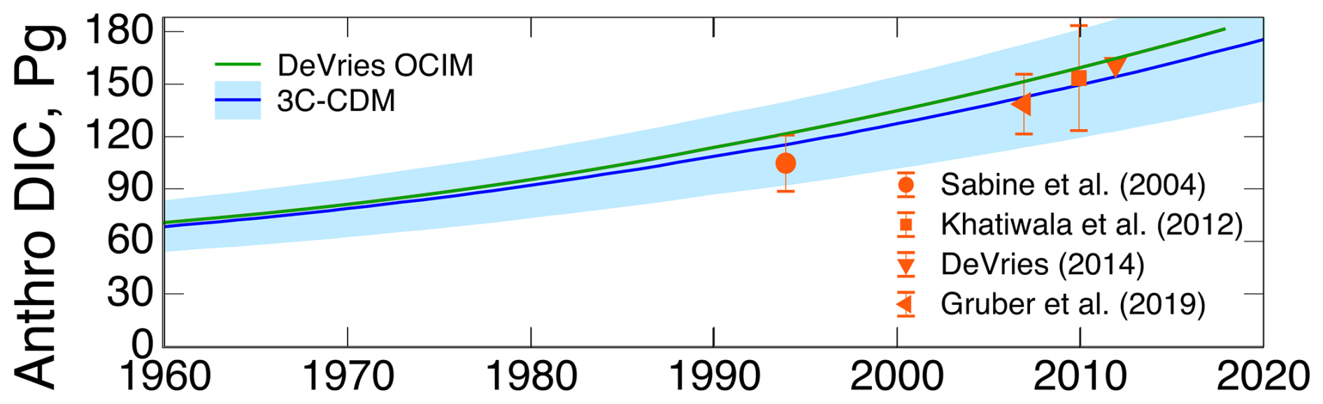
Figure 14 Time dependence of the anthropogenic stock of DIC in the global ocean, as calculated by the Ocean Circulation Inverse Model of DeVries (2022), together with assessed stock of anthropogenic DIC in the global ocean based on measurement campaigns. The figure is based on Fig. 6a of DeVries (2022), with the anthropogenic stock calculated by the 3C-CDM added, including associated 1σ uncertainty. For citations to the measurement data sets, see DeVries (2022).

Figure 15 compares the results from the 3C-CDM with three further observation-derived products. The most direct method (Gruber et al., 2019) determined the rate of increase in the amount of DIC in the global ocean as the difference in ocean carbon stock over the time period 1994–2007 divided by the time between the measurements. The width of the band in the figure denotes that time period. The height of the band in the figure corresponds to the 1σ uncertainty of the Gruber et al. (2019) net uptake flux, reduced from their 2σ estimate for consistency with uncertainties in other data in the figure. Graven et al. (2012) scaled the rate of uptake of anthropogenic carbon to the rate of transfer of excess ¹⁴CO₂ (from nuclear weapons testing in the 1950s and 1960s) from the ML to the DO, which was based on the measured difference in radiocarbon amounts between the 1988–1995 and 2001–2007 time frames; this uptake, like that of anthropogenic CO₂, is now governed principally by transfer from the ML to the DO. The uncertainty range denotes those investigators' estimates of the bounds on the net uptake flux.

Takahashi et al. (2009) evaluated the global net total flux of CO₂ into the ocean (i.e., sum of anthropogenic plus natural) based on local, time-dependent fluxes calculated as the product of the local wind-speed-driven transfer coefficient multiplied by the local partial pressure difference between atmospheric CO₂ and $p_{{\mathrm{CO}}_{\mathrm{2}}}$ of dissolved CO₂ in surface seawater. The CO₂ and $p_{{\mathrm{CO}}_{\mathrm{2}}}$ data were obtained via a time- and space-interpolation method via a 2D diffusion–advection transport equation using a data base of roughly 3 million measurements taken over the period of 1970–2007 and expressed for the reference year 2000, accounting for the increase in atmospheric CO₂ over that time. The local, time-dependent flux was calculated using monthly-mean values of $\mathrm{\Delta }{p}_{{\mathrm{CO}}_{\mathrm{2}}}$ obtained in this way and the mass transport coefficient from reanalysis winds, typically on a 4°×5° grid. That quantity was then integrated over time and space to obtain the global net flux; here it should be noted that the integrand comprised large positive and negative values, reflecting the local and temporal variability of the flux. As this quantity obtained by the integration is the total net flux, it must be decremented by the natural flux (e.g. Gruber et al., 2009), which Takahashi et al. (2009) took as 0.4 Pg yr⁻¹, to obtain the anthropogenic flux. The resulting global mean flux is shown by the open circle, with an accompanying 1σ error estimate, located at the year 2000, the reference year chosen by Takahashi et al. (2009).

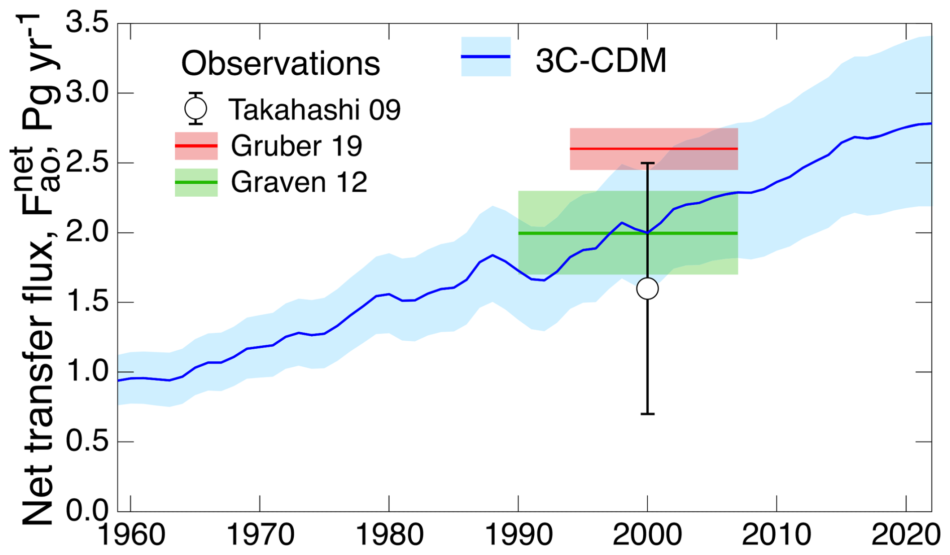
Figure 15 Comparison of net transfer flux of anthropogenic atmospheric CO₂ into the global ocean, as determined by several observation-based studies. The widths of boxes for Gruber et al. (2019) and Graven et al. (2012) denote the time periods over which differences were taken; the heights denote uncertainties, 1σ for Gruber et al. (2019), reduced from their 2σ estimate, and “bounded” for Graven et al. (2012). Uncertainty bar for Takahashi et al. (2009) denotes 1σ uncertainty. Also shown are the results from the 3C-CDM with 1σ uncertainty range.

In sum, this section and Fig. 3 present comparisons of the anthropogenic enhancement to ocean carbon stock, the net anthropogenic atmosphere–ocean flux, and the net atmosphere–ocean transport coefficient, as calculated with the present concentration-driven model with results from multiple other models and available observational data. These comparisons show consistent agreement of the results from this model with the numerous other model calculations and observational data sets examined.

There is also a paucity of ocean radiocarbon data with which to compare the present model results. Additionally, there is the complication of the baseline. The few existing observational studies assume zero anthropogenic ocean carbon prior to the bomb era. Similarly, most model studies examine the changes in stocks only subsequent to 1950 and hence set anthropogenic stocks to zero at that time, in contrast to the 3C-CDM, which is initiated at the preindustrial time (1750). Hence, the changes in stocks are best compared as changes over the post-bomb era. This is achieved in Fig. 16 by offsetting the 3C-CDM results downward by about 150×10²⁶ atoms, the amount of increase in ocean stock in the pre-bomb industrial era (Fig. 8), so that all the curves are forced to coincide at approximately 1957, which was taken as the zero point in previous studies. With that offset, there is fairly good agreement between the 3C-CDM and other model results and between the models and measurement-based assessments, with almost uncanny agreement with the hand-drawn curve of Broecker et al. (1995), which was based largely on measurements in the GEOSECS program (black triangle). A concern in the comparison with the emissions-driven calculation of Naegler and Levin (2006) is that their study shows substantial positive anthropogenic ¹⁴C in the terrestrial biosphere relative to its value in 1957 at all subsequent times, decreasing only slightly after about 1980, whereas the anthropogenic TB stock calculated here as the difference between emissions and stocks in the other compartments (Fig. 9) decreases rather quickly over the post-bomb era, reaching its pre-bomb level by approximately 2004. Resolving this concern will have to await another day.

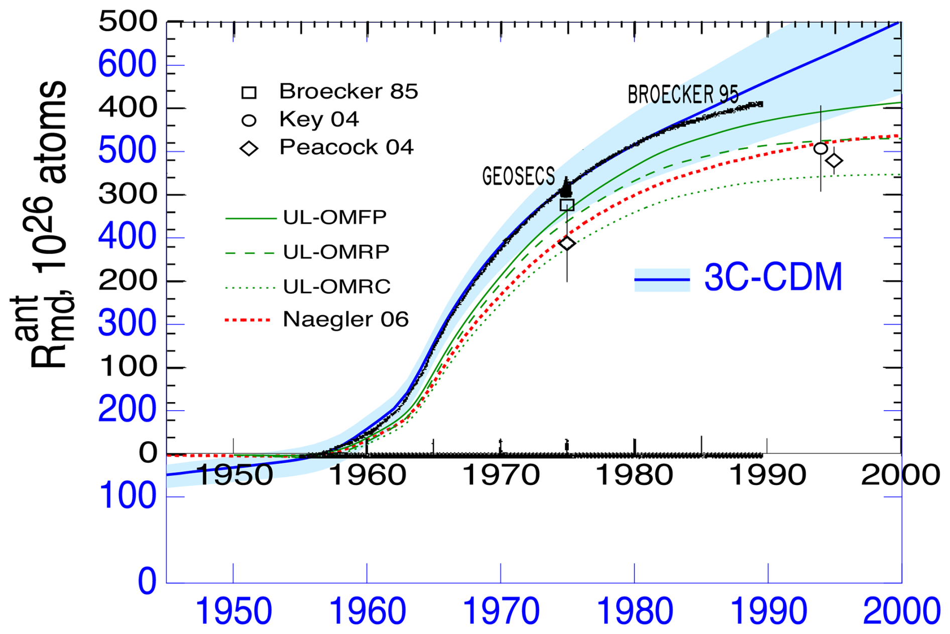
Figure 16 Anthropogenic dissolved inorganic radiocarbon [DI¹⁴C] in the global ocean, as inferred from observations (Broecker et al., 1985; GEOSECS: Broecker et al., 1995; Key et al., 2004; Peacock, 2004) and as calculated with the 3C-CDM, by Naegler and Levin (2006), with several model variants denoted UL from Mouchet (2013), and with a hand-drawn sketch from Broecker et al. (1995). The blue scale denotes 3C-CDM results offset downward by 150×10²⁶ atoms to bring values into coincidence at approximately 1957.

7 Discussion and conclusions

7.1 Discussion

There is keen geophysical and societal interest in the disposition of emissions of anthropogenic CO₂ into the atmosphere in the past, present, and future. Although there are confident measurement-based assessments of atmospheric CO₂ over the Anthropocene, measurements of the fraction of emitted uptake into the ocean are sparse, and there is no confident measure of the amount of CO₂ that has been (or is being) taken up by the terrestrial biosphere. Projections of future atmospheric CO₂ rest entirely on models. As noted wryly by Knutson and Tuleya (2005), “If we had observations of the future, we obviously would trust them more than models, but unfortunately observations of the future are not available at this time”. Consequently, there is an acute need for assessment of the confidence that can be placed in model-based projections. The current approach to modeling the CO₂ budget favors complex carbon cycle models that account for the uptake of atmospheric CO₂ into the ocean and the terrestrial biosphere. These models typically represent the processes that govern uptake and transport of natural and anthropogenic carbon at horizontal scales of the order of 1°, with the number of vertical levels in the ocean of the order of 10. Time steps may be as short as hours. As noted in the Introduction, this approach requires dozens to hundreds of parameters that in turn depend on numerous situational variables, such as temperature and wind speed, and, for uptake into the TB, on water availability and insolation, for numerous vegetation types. As a means of assessing their accuracy, these models are run in emissions-driven mode over time historically over the Anthropocene to obtain the integrated net uptake of emitted CO₂ into the global ocean and the terrestrial biosphere; the difference between emissions and uptake is the anthropogenic increase in atmospheric stock, which can then be compared to atmospheric measurements. Such comparisons, together with comparison of results of multiple models, serve as a measure of the confidence that can be placed in the models and their predictive capability. As an important example, the increase in the mixing ratio of atmospheric CO₂ from 1850 to 2014 was found in the most recent model intercomparison project of the World Climate Research Programme (Coupled Model Intercomparison Project Phase 6; CMIP6) to range from 100 to 135 ppm (Hajima et al., 2024), encompassing the observed increase of 111 ppm. However, such intercomparisons do little to explain the reasons for the departure from observations or the spread among models. Thus, from the perspective of many users of model output, this approach to representing the processes governing the disposition of emitted atmospheric CO₂ into the receiving compartments is opaque: the user of the model results must simply take them “on faith”, with only the vaguest understanding of the method by which the results were obtained, the input parameters employed and their values, the sensitivities to those parameters, the reasons for the departure from observations and differences among the various models, and ultimately the confidence that can be placed in projections obtained with these models.

The present study takes a different tack. Here a simple model is developed that describes the rate and extent of uptake of excess CO₂ by the global ocean. The model has three global compartments: the atmosphere, the mixed-layer ocean, and the deep ocean, with the depth of the ML taken as 100 m. As reported here, the model is run in concentration-driven mode, that is, using the stock of atmospheric CO₂ from measurements to drive the model and examining only the uptake into the two ocean compartments. Although such concentration-driven model runs are only diagnostic, not prognostic, they are capable of yielding considerable insight into the controlling processes and their rates. The 3C-CDM has only two independent parameters: the deposition velocity of low- to intermediate-solubility gases from the atmosphere to the ML (adjusted for the solubility and diffusive properties of CO₂), k_am, and the piston velocity characterizing the rate of water exchange between the ML and the deep ocean, v_p. Importantly, both of these parameters may be considered intrinsic and universal properties of Earth's geophysical system, not specific to CO₂ and not determined by measurements in the CO₂ system. The model also incorporates well-understood and well-characterized equilibria involving the several dissolved inorganic carbon species: CO₂, bicarbonate, and carbonate.

The keystone of the present approach to modeling the uptake of CO₂ by the global ocean is the use of the piston velocity v_p characterizing the rate of exchange of water between the ML and the DO that is equal to the piston velocity governing transport of heat from the ML to the DO. Specifically, this piston velocity is obtained (Sect. 3) from the increase over time in the heat content of the global ocean as determined by multiple measurements; likewise, the uncertainty in the piston velocity, ± 30 %, derives from the uncertainty associated with the heat transport rate between the ML and the DO. The rate of uptake of DIC into the DO in the model thus rests rather firmly on the measured rate of uptake of heat by the global ocean over the time period of 1960 to the present, the same process and the same time period as those governing the bulk of uptake of DIC, thus serving as an ideal surrogate for CO₂ transport.

In the work presented here, the 3C-CDM is used to calculate the rate and extent of uptake of atmospheric CO₂ into the two ocean compartments, with atmospheric CO₂ taken as a forcing function. This application of the model yields a transparent understanding of the processes controlling ocean uptake of CO₂, transport between the atmosphere and the ML and between the ML and the DO, and the basis of the measurement that underlies the values of the two intrinsic parameters. The present study provides a direct connection between uncertainties in the two independent parameters governing the net uptake of excess atmospheric CO₂ by the global ocean and the uncertainty in the net uptake rate. The largest contribution to uncertainty in the rate and extent of uptake of anthropogenic CO₂ by the global ocean, about ± 20 % (1σ) in the year 2022, is due to uncertainty in v_p. As DIC in the ML is in near equilibrium with atmospheric CO₂, uncertainty in the transfer coefficient (deposition velocity) governing the gross rate of uptake of atmospheric CO₂ by the ML, k_am, makes only a minor contribution to the overall uncertainty in the rate of uptake of atmospheric CO₂ by the global ocean. There is some indication in the model results, based on theoretical understanding, that the net transfer coefficient $k_{\mathrm{ao}}^{\mathrm{net}}$ characterizing uptake of excess CO₂ by the global ocean may have decreased slightly (∼ 17 %) over time because of a decrease in solubility of excess CO₂ in the ML and a slight return flux from the DO to the ML. All of this may be compared to the absence of qualitative and quantitative understanding in analysis and interpretation of results from carbon cycle models.

The rate of uptake of excess CO₂ by the global ocean obtained with the 3C-CDM is 2.84 ± 0.6 Pg yr⁻¹ in the year 2022. This value is in essential agreement with the value of 3.0 ± 0.3 Pg yr⁻¹ for 2009–2019 given in an assessment by Gruber et al. (2023) based on multiple methods. The uptake rate determined here corresponds to a net atmosphere–ocean transfer coefficient referred to as excess atmospheric CO₂, $k_{\mathrm{ao}}^{\mathrm{net}}$, of 0.010 ± 0.002 yr⁻¹. The net transfer coefficient is found to be a more sensitive measure compared to the net transfer flux for comparing transfer fluxes across models and for examining the variation in this flux over time within a given model. This intensive quantity exhibits only slight secular variation because of the normalization to the excess atmospheric stock, in contrast to the extensive quantity, the net flux, the time dependence of which is dominated by the increase in atmospheric CO₂. As the net transfer coefficient is much more stable with time than the net transfer flux because it does not increase with increasing atmospheric CO₂, it would seem useful for the net transfer coefficient to be reported in future studies.

The results of the 3C-CDM agree well with measurements of ocean uptake of CO₂ over the time period from the mid-1990s to the early 2010s. The results obtained with the 3C-CDM compare fairly well with the limited available measurements of the anthropogenic increase in ocean DIC stock (Fig. 14) and its rate of increase (Fig. 15), although it must be underscored that such measurements are fraught with difficulty, relying on differences between total stocks and natural stocks or between total stocks at two different time periods. Measurement of the rate of uptake of total CO₂ by the global ocean as the spatial integral of net flux, as was done by Takahashi et al. (2009), would seem to be particularly challenging, in part because the net flux between the atmosphere and the ocean is a small fraction (7 %, global and annual average) of the gross flux (Fig. 5a). The model for radiocarbon also compares well with limited measurements of radiocarbon in the global ocean (Fig. 16).

The comparisons presented in Sect. 6 of the results of the concentration-driven model developed here, 3C-CDM, and those obtained from a variety of complex carbon cycle models to more simple models show surprisingly good agreement, within the roughly ± 20 % uncertainty range associated with present results, in the net atmosphere–ocean transport rate of excess CO₂ over the Anthropocene. Why surprisingly? Because of the vastly different approaches taken – the complexity of carbon cycle models versus the simplicity of the present model. The comparisons with other models span the entire Anthropocene. Despite the multifarious approaches of current CO₂ models and the wide range of $k_{\mathrm{ao}}^{\mathrm{net}}$ calculated from results of model calculations in earlier years of the Anthropocene, the multiple studies converge on a present-day value of $k_{\mathrm{ao}}^{\mathrm{net}}$ equal to about 0.010 ± 0.002 yr⁻¹, or about 1 % yr⁻¹. This convergence, in turn, lends strong support to the use of the piston velocity, which characterizes the rate of exchange of water between the ML, as derived from measurements of the increase in the heat content of the global ocean, as a tracer to describe the rate of uptake of excess CO₂ and to the value of the piston velocity determined here: 7.5 ± 2.2 m yr⁻¹.

The present model study shows that the fraction of anthropogenically emitted CO₂ that is taken up by the global ocean is 25 ± 5 %, at present or as integrated over the industrial period. The present study apportions this uptake, with the fraction of the total net ocean uptake that is transported into the DO being about 80 %. Given the long turnover time characterizing return of water mass and any conservative tracers from the DO to the ML, $k_{\mathrm{dm}}^{-\mathrm{1}}$, or about 450 ± 140 years based on the piston velocity determined here, this uptake into DO may be considered irreversible, at least on the timescale of the Anthropocene thus far. Ultimately, however, on the millennial timescale, the DO would no longer serve as a sink for anthropogenic CO₂.

The 3C-CDM results (Fig. 7c) suggest a slight decrease in $k_{\mathrm{ao}}^{\mathrm{net}}$, from 0.0113 to 0.0093 yr⁻¹, over the period 1900 to the present for v_p= 7.5 m yr⁻¹ and k_am= 0.119 yr⁻¹ (with similar changes for other values of these parameters). Such a slight decrease, which might not otherwise be discernable, is suggested because of a similar decrease in the fractional amount of CO₂ dissolved in the ML over the time period; an increase in return flux from the DO to the ML over this period (Fig. 4) would also contribute to a decrease in $k_{\mathrm{ao}}^{\mathrm{net}}$. From an observational perspective, the difference between emissions and growth of atmospheric stock indicates that over the 1959–2013 time period, the net transfer coefficient from the atmosphere to the combined ocean and TB compartments, $k_{\mathrm{a}-\mathrm{ot}}^{\mathrm{net}}=k_{\mathrm{ao}}^{\mathrm{net}}+k_{\mathrm{at}}^{\mathrm{net}}$, determined as the difference between emissions and atmospheric growth, appears to have decreased substantially from 0.034 to 0.022 yr⁻¹, a decrease of 0.012 yr⁻¹ (Raupach et al., 2014). This decrease is 6-fold greater than the decrease in $k_{\mathrm{ao}}^{\mathrm{net}}$ calculated with the 3C-CDM over the same time period (0.002 yr⁻¹), as shown in Fig. 7c. It remains to be understood whether the large difference is due to a decrease in the terrestrial sink over this time period, an error in the present model, or an error in the observations. It is essential that the reasons for the difference in the two quantities be resolved.

As the version of the model presented here, being concentration driven, is diagnostic, uptake of excess CO₂ into the terrestrial biosphere (TB), either annually or integrated over the Anthropocene, is not directly modeled but, by conservation of matter, is evaluated as the difference between net anthropogenic emissions and the sum of the increase in the atmospheric stock and uptake into the ocean. For both the integrated uptake and the current uptake rates, the fraction of anthropogenic emissions taken up by the TB is 34 ± 5 %, which is comparable to the amount taken up by the global ocean but with a central value that is slightly greater. Representation of uptake of excess CO₂ by the global ocean, as developed here, places a confident constraint on the uptake of excess CO₂ into the TB that will allow confident extension of the model developed here into the emissions-driven mode that must actively represent this uptake. Such extension, to be presented in subsequent papers in this series, will allow the model to be used prognostically rather than diagnostically.

The reliance in this study on the rate of heat uptake by the global ocean underscores the value of continued sustained measurement of the heat content in the global ocean, not just as a measure of change in Earth's energy budget, important in its own right, but also as a surrogate for transport of other tracers, importantly CO₂. Increasing numbers of measurements of global heat content are now being obtained by a flotilla of autonomous profiling buoys under the umbrella of the Argo program, as summarized recently by Cheng et al. (2022). It is to be expected that this expanding data set will result in a decrease in uncertainty in the piston velocity v_p and thus an improved understanding and prognostic capability for the disposition of anthropogenic CO₂ under prospective CO₂ emission profiles. It would, of course, be of enormous value to have a system of well-calibrated autonomous floats, similar to the Argo system, that directly measure ocean DIC content. Any improvements in the knowledge of the piston velocity from such future measurements would only strengthen the confidence that can be placed in the model developed here.

Although the objective of the present study is enhancing understanding of the uptake of excess CO₂ by the global ocean thus far over the Anthropocene, it is of course of interest to ask to what extent the findings of this study might be applicable to the future. As the parameters of the model (the transfer coefficients k_ao and k_md) can be considered properties of Earth's geophysical system and are derived from observations, the values of these quantities would be expected, to first order, to exhibit little or no change in the future. However in the future, they might be subject to change because of the effects of climate change on the controlling processes. Thus, a change in global mean wind speed might enhance the rate of exchange of CO₂ (and other gases) between the atmosphere and the ML. Similarly, changes in ocean circulation due to future climate change might result in a change in heat transport between the ML and the DO, with feedbacks not just on the rate of uptake of DIC by the DO examined here but on Earth's climate system itself.

Finally, although the emphasis here has been on the budget of anthropogenic CO₂, knowledge of the anthropogenic increase in the ocean DIC would also be highly pertinent to the issue of ocean acidification.

7.2 Conclusion

A simple, transparent three-compartment, two-parameter model describing the net transport of atmospheric CO₂ into the global ocean is developed and exercised over the Anthropocene. The two parameters are derived from measurements of global ocean heat uptake in response to increasing atmospheric temperature since 1960 and the deposition velocity of low- to intermediate-solubility gases to ocean water. The results of this model agree closely with available observations and with results of complex carbon cycle models. These findings lead to the conclusion that this simple carbon model represents the net uptake of anthropogenic CO₂ into the global ocean as well as or better than current carbon cycle models. Hence, from the perspective of describing the uptake of anthropogenic CO₂ into the global ocean over the industrial era, this model would meet the needs of many in the research and policy communities concerned with the disposition of anthropogenic CO₂ emissions. Moreover, as the current model is transparent, it readily allows for examination of the dependence of the results on the governing parameters.

Appendix A: Equilibrium solubility of CO₂ in ocean surface water

Figure A1 (a) Dependence of the equilibrium aqueous concentration [DIC] (left axis) and mixed-layer stock S_m (right axis) of dissolved inorganic carbon, i.e., total CO₂, on the atmospheric dry-air mixing ratio $x_{{\mathrm{CO}}_{\mathrm{2}}}$ or stock S_a of CO₂. S_m is calculated for mixed-layer depth z_m= 100 m, ocean temperature of 18 °C, and total alkalinity of 2349 µmol kg${}_{\mathrm{sw}}^{-\mathrm{1}}$. Open circles denote 20-year intervals of atmospheric $x_{{\mathrm{CO}}_{\mathrm{2}}}$ from 1750 to 2010, with points corresponding to the preindustrial (PI) period in 1750, the beginning of contemporaneous measurements of the atmospheric CO₂ mixing ratio in 1959, and the present in 2022. (b) Equilibrium constant for the stocks in the two compartments (Eq. A1). (c) Anthropogenic equilibrium constant (Eq. A2). (d) Differential equilibrium constant (Appendix B, Eq. B20).

The equilibrium solubility of CO₂ in seawater directly affects the distribution of excess CO₂ between the atmospheric and mixed-layer compartments. As noted in the main text, in conjunction with Fig. 1, the equilibrium concentration of DIC in seawater exhibits a sublinear dependence on the CO₂ mixing ratio; i.e., solubility decreases with an increasing CO₂ mixing ratio $x_{{\mathrm{CO}}_{\mathrm{2}}}$. For the analysis presented here, the solubility of CO₂ was calculated with the program CO2SYS (Lewis and Wallace, 1998) for a temperature of 18 °C, representative of the mean for the global ocean, and for alkalinity of 2349 µmol ${\mathrm{kg}}_{\mathrm{sw}}^{-\mathrm{1}}$, selected to obtain preindustrial stock of DIC equal to 900 Pg, as given in previous analyses. Several measures of the equilibrium DIC are shown in Fig. A1 for the entire range of $x_{{\mathrm{CO}}_{\mathrm{2}}}$ over the Anthropocene. The sublinearity of the dependence of DIC on $x_{{\mathrm{CO}}_{\mathrm{2}}}$ over the Anthropocene is manifested in Fig. A1a by the small relative increase in the equilibrium concentration of DIC or in the stock in the ML (depth 100 m), S_m, which is about 7 % versus the much greater relative increase in the stock in the atmosphere S_a of about 50 %. This has the effect of distributing incremental anthropogenic CO₂ increasingly into the atmosphere versus the ocean. The conventional measure of the solubility, the equilibrium constant, and the ratio of the total stocks in the two compartments in equilibrium,

$$\begin{array}{}\text{(A1)}& K_{\mathrm{am}}={\left({\displaystyle \frac{S_{\mathrm{m}}}{S_{\mathrm{a}}}}\right)}_{\mathrm{eq}},\end{array}$$

decreases over this period by about 45 % (Fig. A1b). Perhaps a more relevant measure of the decrease in solubility is the decrease in what may be denoted as the anthropogenic equilibrium constant, which is the ratio of the changes in the two stocks (Fig. A1c):

$$\begin{array}{}\text{(A2)}& K_{\mathrm{am}}^{\mathrm{ant}}={\displaystyle \frac{S_{\mathrm{m}}^{\mathrm{ant}}}{S_{\mathrm{a}}^{\mathrm{ant}}}}.\end{array}$$

Figure A1b, c, and d are drawn to the same relative scale so that the relative changes in the several quantities may be readily perceived. Finally, Fig. A1d shows what is denoted here as the differential equilibrium constant that affects the rate of change in the ML stock for a given rate of change in the atmospheric stock. This differential equilibrium constant is developed in Appendix B.

Appendix B: Transfer fluxes of CO₂ between the atmosphere and the mixed-layer ocean

B1 Kinetics of transfer of CO₂ between gas and aqueous phases

The only CO₂ species in the atmosphere is gaseous CO₂. In solution, however, dissolved CO₂ (commonly denoted as the hydrate carbonic acid, H₂CO₃) dissociates to an equilibrium mixture of H₂CO₃, bicarbonate ion ${\mathrm{HCO}}_{\mathrm{3}}^{-}$, and carbonate ion ${\mathrm{CO}}_{\mathrm{3}}^{\mathrm{2}-}$, with the totality of the three species being denoted as dissolved inorganic carbon (DIC). The equilibria are well characterized, and the kinetics of these dissociation–association reactions are sufficiently rapid for equilibrium to be assumed on the timescales of interest here. Because the only species that exchanges between the solution and the gas phase is CO₂, the rate of this exchange is proportional to the concentration of H₂CO₃, not to that of DIC. This has an effect on the kinetics of the equilibration between gaseous CO₂ and DIC and on how the rates of exchange between the two phases are related to the stocks of CO₂ and DIC, the quantities of principal interest here. This phenomenon is well recognized (e.g., SG06, pp. 330–331) but is nonetheless worth revisiting to develop relations between flux densities (expressed in terms of concentrations) and fluxes (expressed in terms of stocks in the two compartments).

The gross flux density from the atmosphere to the ML is proportional (by the transfer coefficient γ_am) to the volumetric concentration (denoted by square brackets) of gaseous CO₂:

$$\begin{array}{}\text{(B1)}& {\mathit{\varphi }}_{\mathrm{am}}={\mathit{\gamma }}_{\mathrm{am}}\left[{\mathrm{CO}}_{\mathrm{2}}\left(g\right)\right].\end{array}$$

As noted in the text, the coefficient γ_am for this phase transfer process is not a constant (at a given temperature and pressure), as would be the case for a rate coefficient of a chemical reaction, but depends on situational variables, importantly the wind speed that induces convective mixing in the vicinity of the interface. For moderate- to low-solubility gases such as CO₂, the rate-limiting step is mass transport on the water side of the interface. The gross flux density from the ML to the atmosphere is similarly proportional to the concentration of aqueous H₂CO₃:

$$\begin{array}{}\text{(B2)}& {\mathit{\varphi }}_{\mathrm{ma}}={\mathit{\gamma }}_{\mathrm{ma}}\left[{\mathrm{H}}_{\mathrm{2}}{\mathrm{CO}}_{\mathrm{3}}\left(\mathrm{aq}\right)\right].\end{array}$$

The concentrations have a dimension amount per volume, the flux densities φ have a dimension amount per area and time, and the transfer coefficients γ have a dimension amount per area and time per (amount per volume) or length per time (and are thus frequently denoted as a transfer “velocity”). The net flux density is the difference between the gross flux densities:

$$\begin{array}{}\text{(B3)}& {\mathit{\varphi }}_{\mathrm{am},\mathrm{net}}={\mathit{\gamma }}_{\mathrm{am}}\left[{\mathrm{CO}}_{\mathrm{2}}\left(\mathrm{g}\right)\right]-{\mathit{\gamma }}_{\mathrm{ma}}\left[{\mathrm{H}}_{\mathrm{2}}{\mathrm{CO}}_{\mathrm{3}}\left(\mathrm{aq}\right)\right].\end{array}$$

In equilibrium, the net flux ${\mathit{\varphi }}_{\mathrm{am},\mathrm{net}}=\mathrm{0}$, from which it is seen that the two transfer coefficients are related by the equilibrium constant for dissolution of CO₂, commonly denoted as Henry's law solubility constant, which is a function of temperature but is only weakly dependent on solution composition and very weakly on atmospheric pressure and CO₂ partial pressure.

$$\begin{array}{}\text{(B4)}& H_{\mathrm{s}}^{\mathrm{cc}}={\displaystyle \frac{{\mathit{\gamma }}_{\mathrm{am}}}{{\mathit{\gamma }}_{\mathrm{ma}}}}=\left({\displaystyle \frac{{\mathrm{H}}_{\mathrm{2}}{\mathrm{CO}}_{\mathrm{3}}\left(\mathrm{aq}\right)}{{\mathrm{CO}}_{\mathrm{2}}\left(g\right)}}\right)\end{array}$$

Here the notation $H_{\mathrm{s}}^{\mathrm{cc}}$ follows the convention of Sander et al. (2022), wherein the subscript s, denoting solubility, states that the ratio is solution per gas phase, and where the superscripts c and c denote concentrations in both phases. As an equilibrium constant, $H_{\mathrm{s}}^{\mathrm{cc}}$ is not dependent on situational variables such as wind speed, turbulent intensity, and the like, in contrast to the individual transfer coefficients γ_am and γ_ma.

Equation (B4) allows for examination of the kinetics of relaxation of a perturbation from a system initially in equilibrium in order to determine the kinetics of this relaxation. For a closed system initially in equilibrium that is perturbed by the addition of a small incremental amount of CO₂,

$$\begin{array}{}\text{(B5)}& \begin{array}{rl}{\mathit{\varphi }}_{\mathrm{am},\mathrm{net}}& ={\mathit{\gamma }}_{\mathrm{am}}\left({\left[{\mathrm{CO}}_{\mathrm{2}}\left(g\right)\right]}_{\mathrm{0}}+\mathit{\delta }\left[{\mathrm{CO}}_{\mathrm{2}}\left(g\right)\right]\right)\\ & -{\mathit{\gamma }}_{\mathrm{ma}}\left({\left[{\mathrm{H}}_{\mathrm{2}}{\mathrm{CO}}_{\mathrm{3}}\left(\mathrm{aq}\right)\right]}_{\mathrm{0}}+\mathit{\delta }\left[{\mathrm{H}}_{\mathrm{2}}{\mathrm{CO}}_{\mathrm{3}}\left(\mathrm{aq}\right)\right]\right),\end{array}\end{array}$$

where the subscript 0 denotes the initial equilibrium state and where δ denotes the departure from equilibrium, from which

$$\begin{array}{}\text{(B6)}& {\mathit{\varphi }}_{\mathrm{am},\mathrm{net}}={\mathit{\gamma }}_{\mathrm{am}}\mathit{\delta }\left[{\mathrm{CO}}_{\mathrm{2}}\left(\mathrm{g}\right)\right]-{\mathit{\gamma }}_{\mathrm{ma}}\mathit{\delta }\left[{\mathrm{H}}_{\mathrm{2}}{\mathrm{CO}}_{\mathrm{3}}\left(\mathrm{aq}\right)\right].\end{array}$$

By Eq. (B4)

$$\begin{array}{}\text{(B7)}& {\mathit{\varphi }}_{\mathrm{am},\mathrm{net}}={\mathit{\gamma }}_{\mathrm{am}}\left(\mathit{\delta }\left[{\mathrm{CO}}_{\mathrm{2}}\left(g\right)\right]-{\displaystyle \frac{\mathrm{1}}{H_{\mathrm{s}}^{\mathrm{cc}}}}\mathit{\delta }\left[{\mathrm{H}}_{\mathrm{2}}{\mathrm{CO}}_{\mathrm{3}}\left(\mathrm{aq}\right)\right]\right).\end{array}$$

It is desired to express the reverse flux density in terms of [DIC] rather than [H₂CO₃]. Following Sarmiento and Gruber (SG06, p. 330), application of the chain rule

$$\begin{array}{}\text{(B8)}& \mathit{\delta }\left[{\mathrm{H}}_{\mathrm{2}}{\mathrm{CO}}_{\mathrm{3}}\left(\mathrm{aq}\right)\right]={\displaystyle \frac{\mathrm{d}\left[{\mathrm{H}}_{\mathrm{2}}{\mathrm{CO}}_{\mathrm{3}}\left(\mathrm{aq}\right)\right]}{\mathrm{d}\left[\mathrm{DIC}\right]}}\mathit{\delta }\left[\mathrm{DIC}\right]\end{array}$$

together with the definition

$$\begin{array}{}\text{(B9)}& \mathit{\beta }={\displaystyle \frac{\mathrm{d}\left[{\mathrm{H}}_{\mathrm{2}}{\mathrm{CO}}_{\mathrm{3}}\left(\mathrm{aq}\right)\right]}{\mathrm{d}\left[\mathrm{DIC}\right]}}\end{array}$$

yields the expression

$$\begin{array}{}\text{(B10)}& {\mathit{\varphi }}_{\mathrm{am},\mathrm{net}}={\mathit{\gamma }}_{\mathrm{am}}\left(\mathit{\delta }\left[{\mathrm{CO}}_{\mathrm{2}}\left(g\right)\right]-{\displaystyle \frac{\mathit{\beta }}{H_{\mathrm{s}}^{\mathrm{cc}}}}\mathit{\delta }\left[\mathrm{DIC}\right]\right).\end{array}$$

The quantity β is an equilibrium property of the CO₂–DIC system that is generally evaluated numerically from knowledge of the equilibrium constants for dissociation of H₂CO₃. Here, β has the dimension of an equilibrium constant, the ratio of the concentrations of reagent and product, but it is a differential quantity, the ratio of the changes in concentrations resulting from a slight perturbation rather than the ratio of the concentrations themselves, and it is consequently denoted here as a differential equilibrium constant. Importantly, β is dependent on ocean alkalinity and, to a lesser extent, through the equilibrium constants, on salinity and temperature. For the purpose of the present analysis, the alkalinity of seawater is taken as 2349 µmol kg${}_{\mathrm{sw}}^{-\mathrm{1}}$ (consistent with the values of S_m and S_a given for preindustrial conditions in the several prior versions of Fig. 1) with a salinity of 35 and temperature of 18 °C. The dependence of β on the CO₂ mixing ratio over the range of interest for the Anthropocene is shown in Fig. B1 for these conditions.

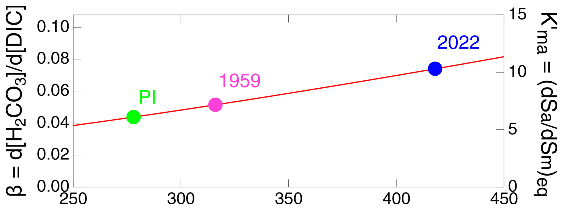
Figure B1 (left axis) Differential equilibrium constant β= d[H₂CO${}_{\mathrm{3}}]/\mathrm{d}$[DIC] denoting equilibrium change in H₂CO₃ concentration per change in DIC concentration as a function of the CO₂ mixing ratio (in dry air) evaluated for seawater alkalinity of 2349 µmol kg${}_{\mathrm{sw}}^{-\mathrm{1}}$, salinity of 35, and temperature of 18 °C. (right axis) Differential equilibrium constant $K{{}^{\prime }}_{\mathrm{ma}}=\mathrm{d}{S}_{\mathrm{a}}/\mathrm{d}{S}_{\mathrm{m}}$, the change in S_a per change in S_m evaluated for the depth of the mixed layer z_m= 100 m, as developed in Appendix B2. Points are also shown corresponding to the preindustrial (PI) time in 1750, the beginning of contemporaneous measurements of atmospheric CO₂ mixing ratio in 1959, and the present in 2022, as in Fig. A1.

B2 Application to transfer of CO₂ between the atmosphere and the global ocean

For consideration of the rates of transfer of CO₂ in the atmosphere–ML system, it is desired to relate rates of change in stocks in the several compartments, expressed in terms of flux F rather than flux density ϕ, to stocks S rather than concentrations C. The flux between the AC and the ML and the stocks in the two compartments are related to the flux density and the two concentrations as

$$\begin{array}{}\text{(B11)}& \begin{array}{rl}& \mathit{\phi }={\displaystyle \frac{F}{A_{\mathrm{o}}}};S_{\mathrm{m}}=A_{\mathrm{o}}{z}_{\mathrm{m}}\left[\mathrm{DIC}\right];\\ & S_{\mathrm{a}}=V_{\mathrm{atm}}\left(T_{\mathrm{sfc}}{p}_{\mathrm{sfc}}\right)\left[{\mathrm{CO}}_{\mathrm{2}}\left(g\right)\right],\end{array}\end{array}$$

where A_o is the area of the global ocean, z_m is the depth of the ML, and $V_{\mathrm{atm}}=N_{\mathrm{air}}R{T}_{\mathrm{sfc}}/p_{\mathrm{sfc}}$, with N_air being the amount (moles) of air in the global atmosphere. Substitution into Eq. (B10) yields the global net flux of CO₂ from the atmosphere to the mixed layer for a small departure from phase equilibrium, δS_a and δS_m:

$$\begin{array}{}\text{(B12)}& F_{\mathrm{am},\mathrm{net}}={\displaystyle \frac{{\mathit{\gamma }}_{\mathrm{am}}{A}_{\mathrm{o}}}{V_{\mathrm{atm}}}}\left(\mathit{\delta }{S}_{\mathrm{a}}-{\displaystyle \frac{V_{\mathrm{atm}}}{{\mathit{\gamma }}_{\mathrm{am}}{A}_{\mathrm{o}}}}{\displaystyle \frac{\mathit{\beta }}{H_{\mathrm{s}}^{\mathrm{cc}}}}\mathit{\delta }{S}_{\mathrm{m}}\right).\end{array}$$

Comparison with Eq. (14) of the main text, which defines the transfer coefficient relating the gross flux of CO₂ from the atmosphere into the global ocean to the atmospheric stock,

$$\begin{array}{}\text{(B13)}& k_{\mathrm{am}}\equiv F_{\mathrm{am}}/S_{\mathrm{a}},\end{array}$$

allows for the identification

$$\begin{array}{}\text{(B14)}& k_{\mathrm{am}}={\displaystyle \frac{{\mathit{\gamma }}_{\mathrm{am}}{A}_{\mathrm{o}}}{V_{\mathrm{atm}}}}\end{array}$$

so that

$$\begin{array}{}\text{(B15)}& F_{\mathrm{am},\mathrm{net}}=k_{\mathrm{am}}\left(\mathit{\delta }{S}_{\mathrm{a}}-K{{}^{\prime }}_{\mathrm{ma}}\mathit{\delta }{S}_{\mathrm{m}}\right),\end{array}$$

where

$$\begin{array}{}\text{(B16)}& K{{}^{\prime }}_{\mathrm{ma}}={\displaystyle \frac{V_{\mathrm{atm}}}{A_{\mathrm{o}}{z}_{\mathrm{m}}}}{\displaystyle \frac{\mathit{\beta }}{H_{\mathrm{s}}^{\mathrm{cc}}}}={\left({\displaystyle \frac{\mathrm{d}{S}_{\mathrm{a}}}{\mathrm{d}{S}_{\mathrm{m}}}}\right)}_{\mathrm{eq}}.\end{array}$$

More generally, with $K{{}^{\prime }}_{\mathrm{ma}}$ viewed as a function of DIC concentration in the ML or, equivalently, S_m,

$$\begin{array}{}\text{(B17)}& F_{\mathrm{am},\mathrm{net}}=k_{\mathrm{am}}\left(S_{\mathrm{a}}-K{{}^{\prime }}_{\mathrm{ma}}\left(S_{\mathrm{m}}\right)S_{\mathrm{m}}\right),\end{array}$$

where the dependence of $K{{}^{\prime }}_{\mathrm{ma}}$ on S_m is explicitly indicated. Like β, $K{{}^{\prime }}_{\mathrm{ma}}$ may be thought of as a differential equilibrium constant but pertinent not to $x_{{\mathrm{CO}}_{\mathrm{2}}}$ and [DIC] but rather to the two stocks. However unlike k_am, which can be considered a geophysical constant, independent of the CO₂ partial pressure or the DIC concentration, $K{{}^{\prime }}_{\mathrm{ma}}$ exhibits a dependence on DIC concentration (or equivalently on $x_{{\mathrm{CO}}_{\mathrm{2}}}$ in equilibrium with the DIC concentration). Moreover, $K{{}^{\prime }}_{\mathrm{ma}}$ depends on the arbitrary choice of the depth taken for the mixed layer z_m. As $K{{}^{\prime }}_{\mathrm{ma}}$ is proportional to β through geophysical constants (and inversely proportional to z_m), it can be shown on the same graph as β, using a proportional axis (Fig. B1), with its numerical value increasing from 5 to 10 over the Anthropocene. For z_m= 100 m, as employed throughout this analysis, the proportionality factor in Eqs. (B12) and (B15), $V_{\mathrm{atm}}/(A_o{z}_{\mathrm{m}}{H}_{\mathrm{s}}^{\mathrm{cc}}$), equals 139.26. $K{{}^{\prime }}_{\mathrm{ma}}$ can equivalently be interpreted as the ratio of the reverse transfer coefficient (from the ML to the AC) to the forward transfer coefficient (from the AC to the ML), $k{{}^{\prime }}_{\mathrm{ma}}$,

$$\begin{array}{}\text{(B18)}& K{{}^{\prime }}_{\mathrm{ma}}={\displaystyle \frac{k{{}^{\prime }}_{\mathrm{ma}}}{k_{\mathrm{am}}}},\end{array}$$

where $k{{}^{\prime }}_{\mathrm{ma}}$ represents the transfer coefficient characterizing the flux from the ML to the AC expressed in terms of the departure of S_m from its equilibrium value as

$$\begin{array}{}\text{(B19)}& F_{\mathrm{ma}}=k{{}^{\prime }}_{\mathrm{ma}}\left(S_{\mathrm{m}}-S_{\mathrm{m},\mathrm{eq}}\right)=K{{}^{\prime }}_{\mathrm{ma}}{k}_{\mathrm{am}}\left(S_{\mathrm{m}}-S_{\mathrm{m},\mathrm{eq}}\right).\end{array}$$

The transfer coefficient $k{{}^{\prime }}_{\mathrm{ma}}$, as defined here, is used in the solution of the differential equations for the evolution of the stocks of CO₂ in response to the anthropogenic perturbation as it automatically takes into account the redistribution of the DIC species associated with transfer of CO₂ from the ML to the AC.

The differential equilibrium constant $K{{}^{\prime }}_{\mathrm{ma}}$ is closely related to a quantity known as the buffer factor or Revelle factor (SG06, p. 332):

$$\begin{array}{}\text{(B20)}& \mathfrak{R}={\left({\displaystyle \frac{\mathrm{dln}{p}_{{\mathrm{CO}}_{\mathrm{2}}}}{\mathrm{dln}\left[\mathrm{DIC}\right]}}\right)}_{\mathrm{eq}},\end{array}$$

which is commonly employed to relate the change in CO₂ partial pressure to the change in DIC, taking into account the equilibria of the DIC species.

$$\begin{array}{}\text{(B21a)}& \begin{array}{rl}K{{}^{\prime }}_{\mathrm{ma}}& ={\left({\displaystyle \frac{\mathrm{d}{S}_{\mathrm{a}}}{\mathrm{d}{S}_{\mathrm{m}}}}\right)}_{\mathrm{eq}}={\left({\displaystyle \frac{S_{\mathrm{a}}}{S_{\mathrm{m}}}}\right)}_{\mathrm{eq}}{\left({\displaystyle \frac{\mathrm{dln}{S}_{\mathrm{a}}}{\mathrm{dln}{S}_{\mathrm{m}}}}\right)}_{\mathrm{eq}}\\ & ={\left({\displaystyle \frac{S_{\mathrm{a}}}{S_{\mathrm{m}}}}\right)}_{\mathrm{eq}}{\left({\displaystyle \frac{\mathrm{dln}{p}_{{\mathrm{CO}}_{\mathrm{2}}}}{\mathrm{dln}\left[\mathrm{DIC}\right]}}\right)}_{\mathrm{eq}}={\left({\displaystyle \frac{S_{\mathrm{a}}}{S_{\mathrm{m}}}}\right)}_{\mathrm{eq}}\mathfrak{R}.\end{array}\end{array}$$

Expressing F_ma by Eq. (B18) thus automatically satisfies this Revelle relation.

The inverse of $K_{\mathrm{ma}}^{\prime }$ (shown in Fig. A1d),

$$\begin{array}{}\text{(B21b)}& K{{}^{\prime }}_{\mathrm{am}}={\left(K{{}^{\prime }}_{\mathrm{ma}}\right)}^{-\mathrm{1}}={\left({\displaystyle \frac{\mathrm{d}{S}_{\mathrm{m}}}{\mathrm{d}{S}_{\mathrm{a}}}}\right)}_{\mathrm{eq}},\end{array}$$

is about an order of magnitude less than K_am. It is $K{{}^{\prime }}_{\mathrm{am}}$ that appears in the differential equation for the evolution of the carbon stock in the ML (Eq. 27), whereas in the differential equation for the evolution of the radiocarbon stock (Eq. 39), it is K_am.