Spring–neap tidal cycles modulate the strength of the carbon source at the estuary–coast interface

Estuaries are dynamic environments with large biogeochemical variability modulated by tides, linking land to the coastal ocean. The carbon cycle at the land–sea interface can be better constrained by increasing the frequency of observations and by identifying the influence of tides with respect to the spring–neap variability. Here, we use FerryBox measurements from a ship of opportunity travelling between two large temperate estuaries in the North Sea and find that the spring–neap tidal cycle drives a large percentage of the biogeochemical variability, in particular in inorganic and organic carbon concentrations at the land–sea interface in the outer estuaries and the adjacent coastal region. Of particular importance to carbon budgeting is the up to 74 % increase (up to 43.0 ± 17.1 mmol C m⁻² d⁻¹) in the strength of the estuarine carbon source to the atmosphere estimated during spring tide in a macrotidal estuary. We describe the biogeochemical processes occurring during both spring and neap tidal stages, their net effect on the partial pressure of carbon dioxide in seawater, and the ratios and fluxes of dissolved inorganic and dissolved organic carbon. Surprisingly, while the two example outer estuaries in this study differ with respect to the timing of the variability, the metabolic state progression, and the observed phytoplankton species distribution, an increase in the strength of the potential carbon source to the atmosphere occurs at both outer estuaries on roughly 14 d cycles, suggesting that this is an underlying characteristic essential for the correct estimation of carbon budgets in tidally driven estuaries and the nearby coastal regions. Understanding the functioning of estuarine systems and quantifying their effect on coastal seas should improve our current biogeochemical models and, therefore, future carbon exchange and budget predictability.

1 Introduction

Coastal seas and estuaries are heterogeneous environments characterized by dynamic biogeochemical variability (Bauer et al., 2013), largely driven by river inputs of water and dissolved and suspended matter from land to the coastal ocean (Burson et al., 2016; Frigstad et al., 2020). Estuaries of large rivers undergo biogeochemical variability on regular short-term (day–night biological cycles and diurnal/semi-diurnal tidal cycles) or medium-term (synodic monthly tidal cycles) scales as well as irregular variability through flood or drought events affecting the flow rate (Regnier et al., 2013; Joesoef et al., 2017; Shen et al., 2019). They are also affected by anthropogenic activities, which can alter ecosystem functioning and carbon and nutrient cycling, and it can take decades for ecosystems to recover (Rewrie et al., 2023b). Thus, while the variability in estuaries and coastal oceans can be difficult to capture, it is essential to attempt to quantify the key processes driving this variability at the land–ocean interface, including how regional physics can affect biogeochemistry (Gattuso et al., 1998; Canuel and Hardison, 2016).

The understanding of carbon cycling at the land–sea interface (LSI) still has large knowledge gaps (Legge et al., 2020), as biogeochemical processes, such as primary production, remineralization, carbonate precipitation and dissolution, and air–sea and sediment–water exchanges, can all alter the carbonate system over short spatial scales (Cai et al., 2021), and tides can add a further layer of complexity. Generally, estuarine waters are a source of CO₂ to the atmosphere (Borges, 2005; Chen and Borges, 2009; Canuel and Hardison, 2016; Riemann et al., 2016; Volta et al., 2016; Hudon et al., 2017), with a global estimate of 0.25 Pg C yr⁻¹ (Cai, 2010). In fact, the amount of carbon released to the atmosphere by estuaries could potentially counteract the carbon absorbed by continental shelves (Laruelle et al., 2010). Spring–neap tidal variability can be an important factor influencing carbon biogeochemistry. Previous studies have addressed this indirectly by focusing on either regenerated nutrients (Webb and D'Elia, 1980) and light and nutrient availability (Cadier et al., 2017) or by investigating the relationship to chlorophyll dynamics (Xing et al., 2021), primary production at shelf edges (Sharples et al., 2007; Lucas et al., 2011), or particle settling in the abyssal seafloor (Turnewitsch et al., 2017). Here, we investigate the influence of spring–neap variability on the estuary–shelf sea interface – specifically how it modulates the lateral and vertical carbon fluxes.

With a good understanding of the underlying processes that govern the variability at the LSI, the carbon biogeochemistry in outer estuaries can be modelled and used to better balance the carbon budgets of shelf seas (Ward et al., 2017; Dai et al., 2022). For example, excluding the effect of estuarine plumes from a computation of the annual CO₂ flux in the southern North Sea increased the sea-to-air flux by 20 % (Schiettecatte et al., 2007). However, challenges remain: for example, a coupled hydrodynamic–ecosystem model used to investigate the impact of coastal acidification in the North Sea was still not able to reproduce pCO₂ correctly (Artioli et al., 2012). Numerous studies have found that the best way to capture and assess the intrinsic estuarine heterogeneity and tidal complexity is to increase observations, so as to correctly identify and characterize the processes in regions where observations already exist (Schiettecatte et al., 2007; Kuliński and Pempkowiak, 2011; Voynova et al., 2015; Regnier et al., 2022). In an estuarine setting, for example, high-frequency observations are particularly important due to the large horizontal gradients present (Kerimoglu et al., 2018; Cai et al., 2021). Furthermore, the difference in the tidal energy between spring and neap tides influences the location and intensity of mixing processes (Chegini et al., 2020). A high observational frequency that is able to capture both spatial and temporal variability can be achieved with ship-of-opportunity (SOO) measurements (Jiang et al., 2019).

In a recent study, Macovei et al. (2022) observed high seawater pCO₂ outside the Humber River estuary as well as variability that seemed to match the spring–neap tidal cycles. However, the authors found that, while the Copernicus Marine Environment biogeochemical shelf sea model (Butenschön et al., 2016) captured the pCO₂ spatial distribution in the central North Sea, in the nearshore, outer-estuary region, neither the overall pCO₂ levels nor the variability in pCO₂ was accurately reproduced. Furthermore, not accounting for the influence of estuaries in coastal regional models, as evidenced by Canuel and Hardison (2016), raises the uncertainty in the carbon budget estimations and can lead to erroneous results. A recent study showed that rivers perturb the coastal carbon cycle to a larger extent offshore than previously considered (Lacroix et al., 2021) and that they can influence coastal regions via changes in estuarine discharge (Garvine and Whitney, 2006; Voynova et al., 2017; Kerimoglu et al., 2020). In addition, the land-based inputs and the partitioning between the inorganic and organic carbon forms is needed for regional budget calculations (Kitidis et al., 2019). In this context, this study examines the tidally driven spring–neap biogeochemical variability in the outer estuaries of two large European rivers, characterizes this variability with respect to the carbon concentrations and fluxes at the LSI, and quantifies the largely unaccounted for impact on regional carbon budget assessments.

2 Methods

2.1 Study area

The North Sea as a whole has previously been characterized as an important carbon sink (Thomas et al., 2005); however, recently, driven by summertime biological activity, a decrease in the buffer capacity, and a diminishing efficiency of the continental shelf pump (Tsunogai et al., 1999), its carbon uptake capacity has weakened (Lorkowski et al., 2012; Clargo et al., 2015; Bourgeois et al., 2016). The seawater pCO₂ in the North Sea was found to be increasing at a faster rate than the atmospheric one, mainly driven by non-thermal effects in the summer months, shifting the carbon uptake– release boundary northwards (Macovei et al., 2021a). This affects the central North Sea, which separates the northern region – as a dominant sink – from the southern region – as an overall source of CO₂ to the atmosphere. This creates a fragile balance regarding the direction of the carbon dioxide flux, which depends on the dominance of thermal or biological forcing (Hartman et al., 2019; Kitidis et al., 2019). Therefore, the North Sea is an ideal location to investigate this variability at the LSI using long-term and high-frequency observations. The MS HAFNIA SEAWAYS (DFDS seaways, Copenhagen, Denmark) is a cargo vessel that regularly transited the North Sea between 2014 and 2018. The ship was equipped with a FerryBox as part of the Coastal Observing System for Northern and Arctic Seas (COSYNA; Baschek et al., 2017) and travelled between Immingham (UK) and Cuxhaven (Germany). These ports are located within the outer estuaries of the Humber and Elbe rivers, respectively, two tidally driven estuaries with different characteristics and catchment regions (Fig. 1). While the carbon dynamics in the central North Sea have been previously assessed (Macovei et al., 2021a), this work is focused on the land–sea interface – in particular the two temperate estuaries and their adjacent coastal regions specified in Fig. 1c and d.

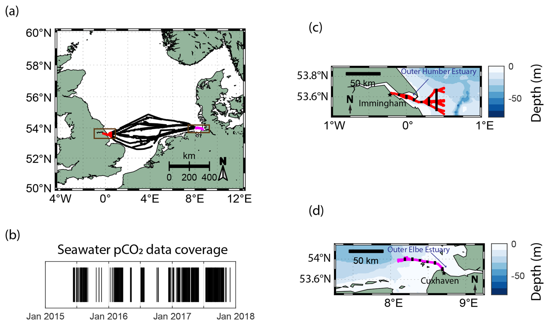
Figure 1 The SOO routes (a) and the temporal pCO₂ data coverage (b) of MS HAFNIA SEAWAYS travelling in the North Sea between 2015 and the end of 2017. Black markers in panel (b) indicate the available measurements during this period. Zoomed-in views of the locations of the near-shore measurements (brown boxes in panel a) used in this study and the NOAA ETOPO2 bathymetry near (c) Immingham (UK; in red) and (d) Cuxhaven (Germany; in magenta) are also shown. In panels (c) and (d), the locations of the selected samples for the box plot analysis in Figs. 3 and 5 are indicated using black markers.

The Humber River catchment extends over 24 000 km², and its average river discharge (1990–1993) is England's largest at 250 m³ s⁻¹ (Sanders et al., 1997). Its geology is Carboniferous limestone in the west and Permian and Triassic sandstone in the east, while the overlying Quaternary deposits are mostly clays (Jarvie et al., 1997b). The catchment area is a mix of industrialized, agricultural, and urban areas, and the anthropogenically influenced runoff affects the biogeochemical processes in the estuary (Jarvie et al., 1997a). Between 70 % and 80 % of the catchment is arable land or grassland, and the agricultural practices cause the nitrate concentrations in the surface waters to frequently exceed the 50 mg L⁻¹ EU Nitrates Directive standard (Cave et al., 2003). The excess nutrients are carried to the estuary, which starts at Trent Falls, about 60 km inland from the coast, but estuarine primary production is strongly light-limited by high turbidity (Jickells et al., 2000). Therefore, most nutrients are likely transported offshore, rather than being assimilated in the estuary. The estuary outflows of the Humber and other British east coast rivers form the East Anglian plume, which influences primary production in the southern North Sea further offshore of the immediate river and estuary outflows, reaching as far as the Southern Bight of the North Sea (Dyer and Moffat, 1998; Weston et al., 2004). The effluent from industrial sources increases the biological oxygen demand in the estuary; therefore, the Humber estuary oxygen concentrations are low (Cave et al., 2003). Tides in the Humber Estuary are semi-diurnal, and the tidal range of up to 7.2 m makes it a macrotidal and well-mixed estuary.

The Elbe River catchment extends over 148 000 km², with an average river discharge (2005–2007) of 730 m³ s⁻¹, making it one of Europe's largest rivers (Schlarbaum et al., 2010). The source of the river is found in Czechia in the Giant Mountains, which are primarily comprised of granite. The Elbe then flows through sandstone mountains before crossing the flat fertile marshlands of north Germany. River water chemistry is strongly correlated with the watershed geology (Newton et al., 1987); therefore, one would expect the alkalinity in the Elbe to be lower than in the Humber River, which flows through limestone bedrock. However, Hartmann (2009) found that the carbonate abundance in silicate-dominated geology is also important. In addition, the erosion rate, mean annual temperature, catchment area, and soil regolith thickness can all influence the river carbon chemistry (Lehmann et al., 2023). The anthropogenic pressure in the Elbe watershed is high, with most of the catchment being dominated by agricultural land use (Quiel et al., 2011). While water quality has improved since the 1980s (Dähnke et al., 2008; Amann et al., 2012; Rewrie et al., 2023b), the measures have disproportionately reduced the phosphorus input, so the current nutrient load has an increased nitrogen-to-phosphorus ratio (Geerts et al., 2013). The Elbe Estuary extends from the Geesthacht Weir to the mouth of the estuary at Cuxhaven, Germany, a further 141 km downstream. The large Port of Hamburg, situated in the upper estuary, also increases the anthropogenic pressure in the estuary due to regular dredging and industrial activities that facilitate the development of oxygen-depleted zones (Geerts et al., 2017). Tides are semi-diurnal and have a tidal range of up to 4 m. Therefore, the Elbe Estuary falls between a meso- and macrotidal estuary and the salinity profiles classify it as a partially mixed to well-mixed estuary (Kerner, 2007).

2.2 FerryBox measurements

A FerryBox is a modular automated measurement system that can be installed on SOOs or fixed stations to provide high-frequency observations of sea surface waters (Petersen, 2014). Their characteristics make them ideal as autonomous biogeochemical observatories on moving platforms (Petersen and Colijn, 2017). FerryBox systems are mature platforms with a well-established FerryBox community and EuroGOOS Task Team. Many publications have used FerryBox data in our study area (Voynova et al., 2019; Kerimoglu et al., 2020; Macovei et al., 2021a), and Chegini et al. (2020), for example, used FerryBox measurements to identify and characterize the effect of spring and neap tides to the stratification regime in the German Bight. A suite of instruments were installed on the MS HAFNIA SEAWAYS (Table 1). Quality-controlled temperature, salinity, and pCO₂ data obtained by this SOO are now publicly available on the PANGAEA repository (https://doi.org/10.1594/PANGAEA.930383, Macovei et al., 2021c) and have been used in a previous study evaluating surface seawater pCO₂ trends (Macovei et al., 2021a). All other data are currently available in the European FerryBox Database (https://ferrydata.hereon.de, last access: 26 March 2025) and on the COSYNA data web portal (Baschek et al., 2017).

Table 1 The FerryBox-integrated instruments installed on MS HAFNIA SEAWAYS that were employed for measurements between 2015 and 2017 and used in this study.

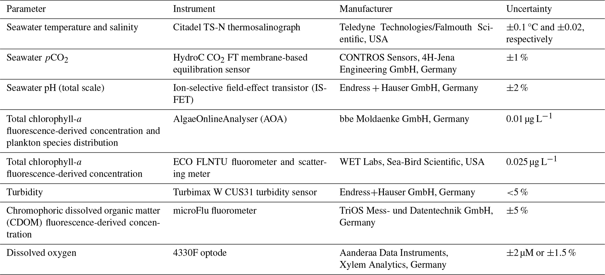
During the data collection period (2.5 years), 53 maintenance visits were performed. The flow cells of the sensors were cleaned and, if deemed necessary, the sensors were replaced. New sensors are always calibrated by the manufacturer, with documentation provided. The temperature and salinity sensor, the WET Labs chlorophyll sensor, and the chromophoric dissolved organic matter (CDOM) sensor were not changed. The pCO₂ sensor was changed four times, and appropriate data processing methods were applied, as described by Macovei et al. (2021b), to ensure a span-drift correction; moreover the sensor was quality-controlled (Macovei et al., 2021c) to ensure that no abrupt changes in the data occurred. The ion-selective field-effect transistor pH sensor was changed once, the AlgaeOnlineAnalyser (AOA) chlorophyll sensor was changed three times, and the oxygen optode was changed three times, with verification samples for the latter instrument collected 22 times.

The FerryBox system starts measurements automatically based on the GPS location after departure from port. As some instruments need time to reach optimal functioning, we only use data from the ship's journeys arriving to port. The arrival time into ports was consistent, irrespective of the tidal stage or sea level (Fig. 2a, b). As high and low tides progress every day (12.5 h cycle), long time series, like those used in this study, will likely include all tidal stages with no bias. All of the statistical analyses were carried out using original, quality-controlled data. There are sufficient data without gaps to capture consecutive spring and neap tide events and also to characterize the typical state of the system during the spring and neap tidal stages.

2.3 Processing of FerryBox data

The turbidity sensor was calibrated using discrete samples that were collected by the auto-sampler installed on board the vessel and measured in the laboratory between February 2016 and July 2017 (R²=0.92, n=19). Measurements at the upper limit of detection or above were discarded.

The FerryBox was equipped with a bbe Moldaenke GmbH AOA, which provided valuable information about the relative distribution of plankton classes contributing to the total pigment signal (Wiltshire et al., 1998). The sensor can usually differentiate between diatoms, green algae, blue-green algae, and cryptophytes. However, the total chlorophyll was likely overestimated by this instrument. We also measured total chlorophyll with a WET Labs sensor. We compared the WET Labs measurements with laboratory high-performance liquid chromatography (HPLC) measurements, collected in March 2016 from the onboard autosampler (R²=0.94, n=4). The AOA measurements were then calibrated to the corrected WET Labs measurements. As four different AOA instruments were used during the study period, linear relationships were calculated for each instrument deployment in each of the two outer estuaries, with coefficients of determination ranging from 0.52 to 0.95 (details in Fig. S1).

Between February 2016 and November 2017, the performance of the ISFET pH sensor was evaluated 11 times during maintenance visits by measuring buffer solutions with pH values of 7.0 and 9.0. Using the time regression of the difference between the measurements and the standards, we assessed that the instrument exhibited a drift of 0.00045 pH units per day, which we corrected for before reporting the final results.

We used the MATLAB CO2SYS toolbox (van Heuven et al., 2011) with the Cai and Wang (1998) K₁ and K₂ dissociation constants, which are appropriate for salinities as low as 0, and the Dickson et al. (1990) K SO₄ constant to calculate dissolved inorganic carbon (DIC) concentrations from pCO₂ and pH. We converted the ISFET pH measured on the total scale to the NBS scale before calculating, in order to fit the requirements of the dissociation constants used. This conversion was performed using CO2SYS, with the associated values of temperature, salinity, and pCO₂ for each pH value. To compare with the dissolved organic carbon (DOC) concentrations, the DIC concentrations were converted to micromoles per litre (µmol L⁻¹) using the Gibbs Seawater toolbox for MATLAB (McDougall and Barker, 2011). An empirical relationship between CDOM fluorescence, expressed on the quinine sulfate unit (QSU) scale, and the DOC concentration was used to calculate the latter. This relationship was based on the measurements of DOC concentrations and CDOM fluorescence during the HE407 research cruise with RV Heincke, which took place in the outer Elbe Estuary and German Bight in August 2013. Water samples were analysed in the laboratory, and the following linear relationship (R²=0.67, n=10) was found with results from the Trios microFlu CDOM fluorometer integrated into the FerryBox on board: $\mathrm{DOC}\left[\mathrm{\mu }\mathrm{mol}{\mathrm{L}}^{-\mathrm{1}}\right]=\mathrm{10.75}\times \mathrm{CDOM}\left[\mathrm{\mu }\mathrm{g}{\mathrm{L}}^{-\mathrm{1}}\right]+\mathrm{162.06}$. While we acknowledge the limitations of using an empirical relationship based on a single cruise, this relationship is close to other literature references discussed below, and the resulting DOC concentrations fall within the range of direct water sample measurements made by the Flussgebietsgemeinschaft Elbe. Converting the proxy CDOM results into estuarine DOC concentrations is useful for understanding the partitioning of dissolved carbon between the inorganic and organic fractions.

2.4 Additional data

Sea level data at the Immingham Docks were obtained from the British Oceanographic Data Centre (https://www.bodc.ac.uk/data/hosted_data_systems/sea_level/uk_tide_gauge_network/processed/, last access: 26 March 2025). Sea level data at the Cuxhaven Pier were obtained from the German Federal Waterways and Shipping Administration (WSV), communicated by the German Federal Institute of Hydrology (BfG) (https://www.pegelonline.wsv.de/gast/stammdaten?pegelnr=5990020, last access: 26 March 2025). The reporting frequency of the datasets was 15 and 1 min, respectively. In order to extract the spring–neap tidal cycle, sea level data were processed by running a moving maximum and a moving minimum calculation with a 100 h window (to smooth the time series). The highest (lowest) difference between the 100 h smoothed maximum and minimum sea level occurs during spring (neap) tides, with a recurrence interval approximately matching the literature value of 14.77 d (Kvale, 2006). The times of the spring and neap tides were identified with a peak search function on the smoothed tidal range. Data were categorized by assigning measurements taken within ±25 h of the identified peaks to spring tide or neap tide periods, respectively.

We cross-checked our findings with fixed-point salinity data from the Cuxhaven observing station, equipped with a FerryBox and situated at the outflow of the Elbe Estuary into the North Sea. This station is now also part of the ICOS-D network (since 2023) and has been successfully used by Rewrie et al. (2025) to estimate primary production and net ecosystem metabolism at the LSI. The time span of this dataset is 2020–2022, after the Cuxhaven FerryBox station was equipped with a CDOM sensor. While this is a few years later than the MS HAFNIA SEAWAYS dataset, the comparison to a station with a high temporal resolution is valuable. To the best of our knowledge, there is no equivalent biogeochemical observing station in the Humber Estuary.

Atmospheric carbon dioxide measurements were obtained from the Mace Head observatory in Ireland (World Data Centre for Greenhouse Gases, 2020). These are reported as dry-air mole fraction (xCO₂), expressed in parts per million (ppm). We used barometric pressure, dew point temperature, and 10 m wind speed from the ERA5 reanalysis product (Hersbach et al., 2018) selected for the closest pixel to the Humber Estuary region, as provided by the Copernicus Climate Data Store (https://cds.climate.copernicus.eu, last access: 26 March 2025). When estimating sea-to-air carbon fluxes, we calculated average values of the years 2015–2017 for the required input terms. The atmospheric xCO₂ was converted to pCO₂ using the saturated water vapour pressure formula from Alduchov and Eskridge (1996).

Finally, we used the DriftApp Tool of the coastMap geoportal (https://hcdc.hereon.de/drift-now/, last access: 26 March 2025; available under a CC BY-NC 4.0 licence) to simulate water mass movement in our study areas. This application specifies drift trajectories using the PELLETS-2D Lagrangian transport program (Callies et al., 2011). Drift simulations are based on 2D marine currents extracted from archived output of the 3D hydrodynamic model BSHcmod that is run operationally at the Federal Maritime and Hydrographic Agency of Germany (BSH). The tool has successfully been used for particle and water mass tracking applications (Callies, 2021; Callies et al., 2021). We simulated 24 h backward trajectories from selected locations in the two outer estuaries starting both at the high and low tides during spring and neap tide conditions, which we selected from the sea level data.

3 Results

The frequency of the repeating ship journeys to each port is too low to resolve the semi-diurnal high and low tides that characterize the two estuaries, but it is high enough to provide data during each stage of a spring–neap tidal cycle. Our observations showed cyclical variability, so we applied spectral analysis on our dataset using the fast Fourier transform method with the “fft” MATLAB function. The signal with the highest power had a period of 14.5 d for the Humber Estuary and 14.1 d for the Elbe Estuary, indicating that spring–neap cycling is the main mode of pCO₂ variability for SOO data in these regions (Fig. 2c). We applied the same analysis to continuous (1 min resolution) salinity data from the Cuxhaven observing station with the dominant period at 12.4 h, indicating that the semi-diurnal tides dominate the variability at the resolution provided by the station. After filtering out the high-frequency data with a 3.5 d moving average, the dominant frequency in the power spectral density plot occurred at 14.5 d revealing the spring–neap-driven biogeochemical variability in the station data too (Fig. 2d). Further examples of Cuxhaven station data demonstrate fortnightly variability in biogeochemical parameters, such as CDOM (Fig. 2e) and turbidity (Fig. 2f). For a similar investigation of arrival time and spectral analysis in the outer Humber Estuary and further data from the Cuxhaven station, see the Supplement (Fig. S2).

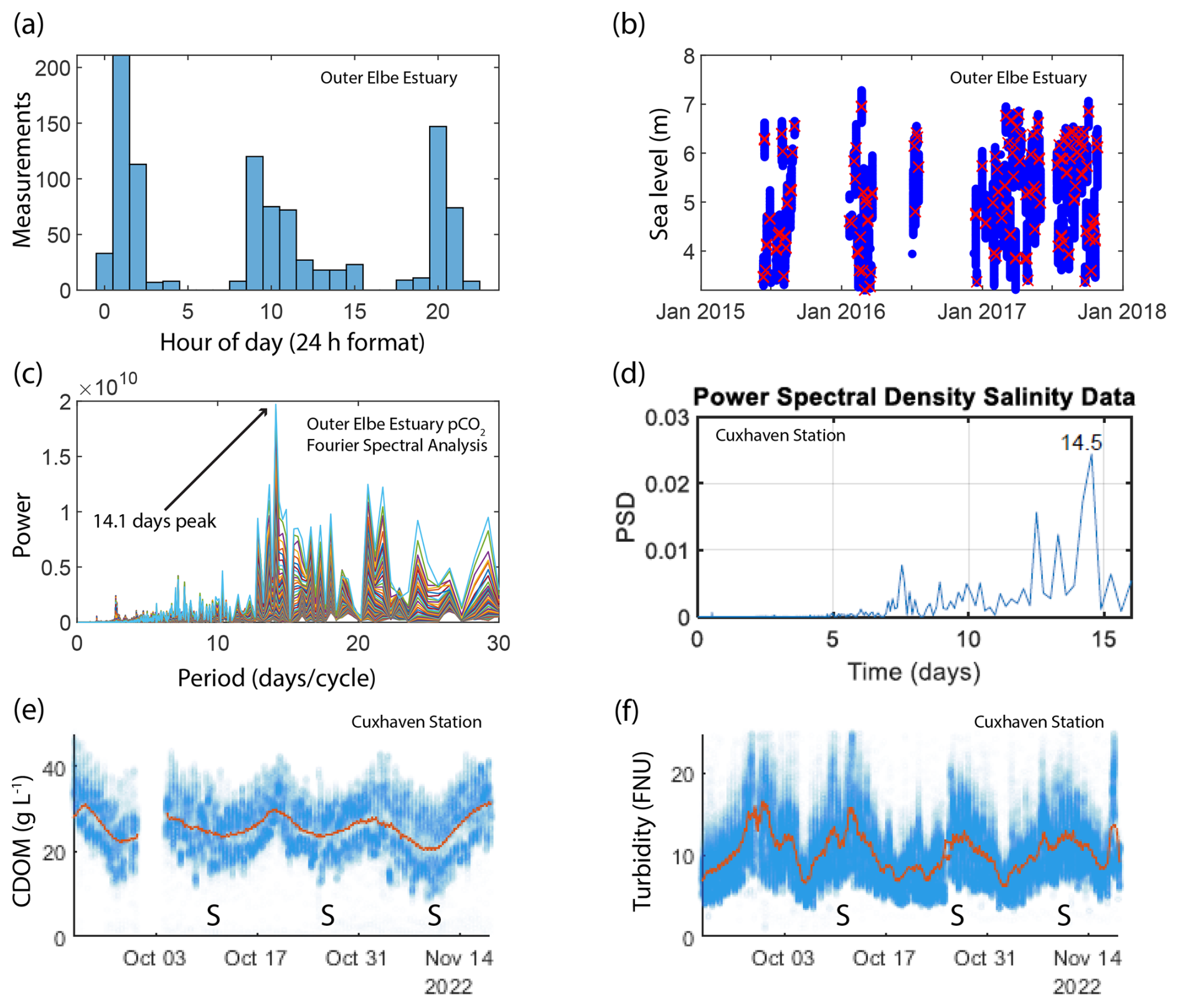
Figure 2 (a) Histogram showing the ship arrival time in Cuxhaven port in the outer Elbe Estuary. (b) The sea level at the arrival time (red crosses) compared to the usual sea level range (blue dots) in the outer Elbe Estuary. (c) The power versus period (inverse of frequency) plot resulting from a fast Fourier transform analysis on pCO₂ SOO data in the outer Elbe Estuary. (d) A Fourier analysis of the salinity data from the Cuxhaven fixed-point measurement station in the outer Elbe Estuary performed on a 3.5 d moving average to filter out the high frequencies, which would produce a strong 12.5 h peak. The resulting power spectral density plot shows a peak at 14.5 d. We also show the cyclical biweekly biogeochemical variability at Cuxhaven by selecting observations from a 2-month period in autumn 2022. The CDOM (e) and turbidity (f) observations are shown using blue markers, whereas a 3.5 d moving average is shown in orange. Spring tides are indicated using “S” on the time axes.

3.1 Tidally controlled biogeochemistry in the Humber Estuary and adjacent coast

The SOO observations reveal that biogeochemical parameters in the outer Humber Estuary vary according to the spring–neap tidal cycle. We selected all available measurements (Fig. 1c) around six positions based on the longitude (±0.005° around every 0.1°) and further split and sorted them into times when spring or neap tides are expected (Fig. 3). The chosen locations demonstrate the gradients from port, through the outer estuary, and to the adjacent coastal sea waters. For other methods of selecting the data with similar results, see Fig. S3. Statistical differences between groups are assessed using a Welch t test (“ttest2” MATLAB function), with a rather strict significance level of 0.01 to avoid false positives. This statistical method tests the null hypothesis that two populations, with not necessarily equal variances, have equal means, and it is appropriate to compare our spring and neap tide groups.

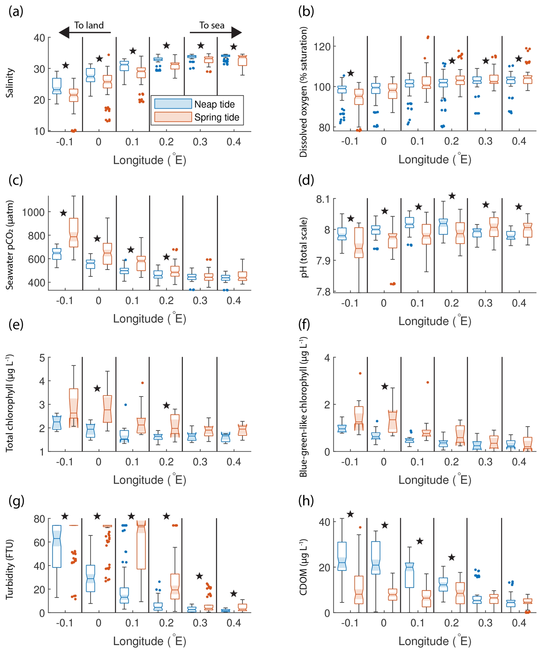
Figure 3 Box plots of salinity (a), dissolved oxygen saturation (b), seawater pCO₂ (c), pH (d), total chlorophyll concentration (e), blue-green-like chlorophyll concentration (f), turbidity (g), and CDOM (h) grouped in six regions in the outer Humber Estuary, comparing the neap (blue) and spring (red) tide measurements. The box plots display the median, interquartile range, and outliers. When the notches of two box plots do not overlap, they have different medians at the 5 % significance level. We also indicate the statistical difference between spring and neap tide measurements using symbols above the specific pair. Spring tide turbidity values are above the upper limit of detection in the westernmost two box plots in panel (g) and are, therefore, reported as this maximum value, without variance. Star symbols indicate statistically significant differences between spring and neap tide groups assessed with Welch's t test.

Significant differences between the mean spring tide and the mean neap tide results indicated that salinity was significantly lower during spring tide than during neap tide at all locations (Fig. 3a). Both the spring and neap tide datasets selected captured various stages of the semi-diurnal tidal cycle. For example, at the most upstream location, the spring tide salinity was 18.9 ± 0.3 during low tides and 22.6 ± 0.7 during high tides, whereas the neap tide salinity was 22.6 ± 2.4 during low tides and 25.8 ± 3.2 during high tides. Stronger oxygen undersaturation was observed during spring tides (Fig. 3b). Seawater pCO₂ was significantly higher during spring tide at the four westernmost locations in the outer Humber Estuary, with a maximum median value of 787 µatm (interquartile range of 700 to 844 µatm) (Fig. 3c). At the same four locations, the spring tide pH was significantly lower than the neap tide pH, while, surprisingly, the spring tide pH was significantly higher than neap tide values at the easternmost offshore locations (Fig. 3d). The total chlorophyll-a (Fig. 3e) and blue-green signal from the AOA measurements (Fig. 3f) had a high variance but generally presented higher values during spring tides. Turbidity was significantly higher at spring tide than at neap tide at all chosen locations (Fig. 3g). CDOM had a reverse pattern to turbidity and pCO₂, with spring tide values significantly lower than neap tide values at the four westernmost locations (Fig. 3h). Most variables show a gradient between the estuary and the offshore regions. Salinity medians (ranging from 21 to 31) were lower than the North Sea salinity (ranging from 32 to 35), and a low-salinity plume was observed up to 0.2° E, or 7 km offshore of the estuary mouth. There was also a west-to-east gradient in the oxygen saturation measurements. Turbidity, total and blue-green-like chlorophyll-a, and CDOM were all lower offshore than in the estuary. In fact, during spring tide, turbidity measurements exceeded the upper limit of the sensor (∼ 74 FTU, formazin turbidity units).

The results presented in Fig. 3 show that the outer Humber Estuary experiences two distinct states, depending on the spring–neap tidal cycle. The advantage of the repeating ship journeys is that the transition between these states and the cyclical variability were observed. In order to show this, we chose a 2-month period with relatively good data coverage and present the Humber Estuary data as a Hovmöller plot (Fig. 4). We show the same variables as in Fig. 3 and overlay a line plot of the tidal range to co-locate the spring–neap tidal cycle with the observed changes in the biogeochemical parameters. This addition helps to show the relationship between the physical forcing and the biogeochemical response.

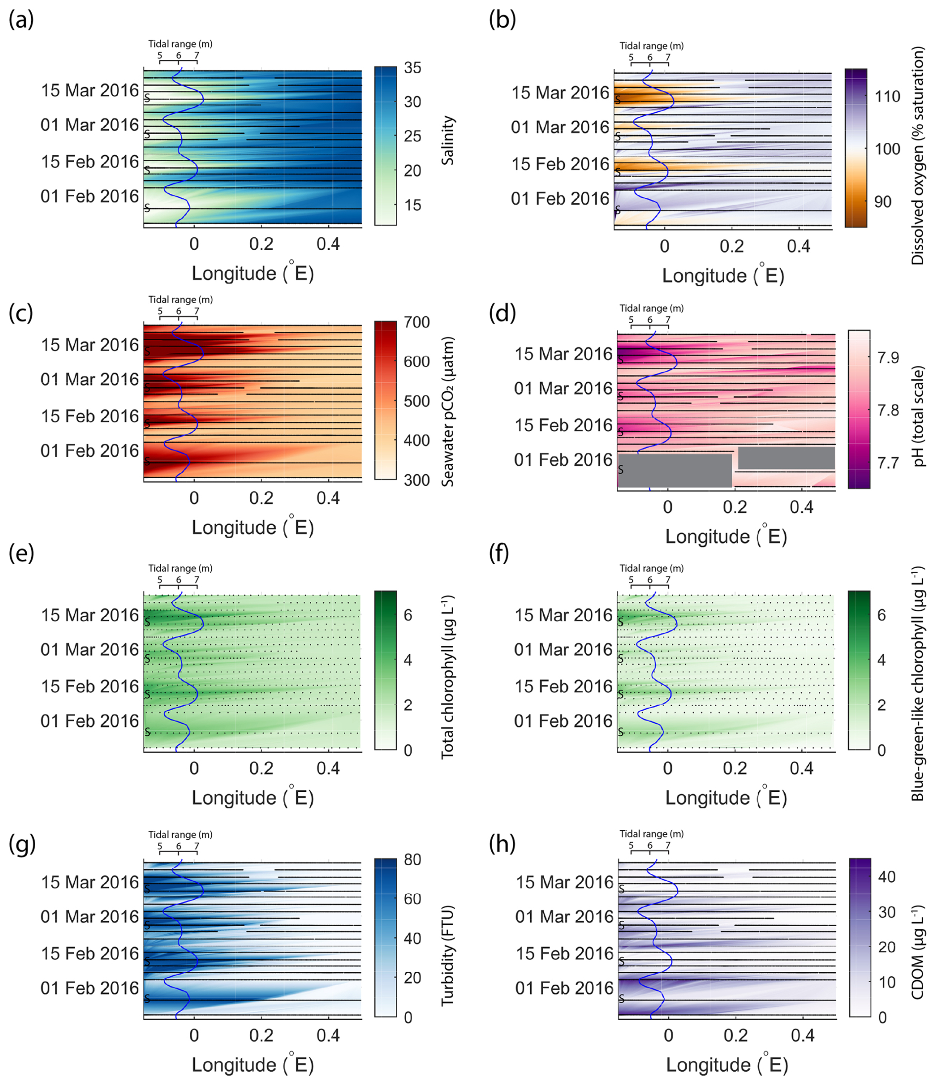
Figure 4 An example of fortnightly variability in biogeochemical parameters in the outer Humber Estuary matching the spring–neap tidal cycle. The time and longitude coordinates of the measurements are shown in black. The tidal range is shown using the blue line, and spring tides are indicated using “S”. Large data gaps are masked out with grey boxes. The variables shown are salinity (a), dissolved oxygen saturation (b), pCO₂ (c), pH (d), total chlorophyll (e), blue-green-like chlorophyll (f), turbidity (g), and CDOM (h).

In the 2-month period shown in Fig. 4, four spring tides and four neap tides occurred. The transition between the two tidal states was influenced via the tidal range by modulating the strength of the estuarine influence. For example, the offshore extent of the spring-tide-driven conditions and the maximum levels reached during the less-pronounced spring tide event (24 February 2016) were smaller for most variables presented here, except for salinity and pCO₂. Similar to the median conditions in 2015–2017 (Fig. 3), CDOM was higher during neap tide. Especially further upstream in the estuary, the physical and biogeochemical variability was high and was correlated with the spring–neap tidal cycles. From neap to spring tide, the seawater changed from a salinity of 15, oxygen undersaturation, and high carbon dioxide oversaturation to a salinity higher than 25, oxygen oversaturation, and carbon dioxide close to atmospheric balance. In the estuary region, turbidity was below 20 FTU during neap tides and above the detection limit of 74 FTU during spring tides.

3.2 Tidally controlled biogeochemistry in the outer Elbe Estuary

The ship stopped at the mouth of the Elbe Estuary at Cuxhaven (Fig. 1d), but we were able to observe the estuarine signal: the median of the salinity measurements at the easternmost location was low, at around 19, for both the spring and neap tide (Fig. 5a). This region has been described as the outer Elbe Estuary (Rewrie et al., 2023b) and is known to feature rapid changes in pCO₂ with changing salinity (Brasse et al., 2002). The high interquartile range at this location makes differentiating spring and neap tide measurements more difficult. Salinity increased offshore off the estuary outflow; however, unlike in the Humber, statistically significant lower salinity was observed during neap tides. The medians of the oxygen measurements were higher than 100 % saturation, except in the region closest to Cuxhaven, where a significant difference between spring and neap tide oxygen was observed, with neap tide oxygen being significantly lower (Fig. 5b). Seawater pCO₂ was generally higher towards the estuary, and it was above the atmospheric level, with medians ranging from 422 to 594 µatm. Unlike in the Humber, there was no difference between the spring and neap tide in seawater pCO₂ in the outer Elbe Estuary, except at two locations (8.39 and 8.69° E) where the Welch t test showed that neap tide pCO₂ values were significantly higher than the spring tide pCO₂ values (Fig. 5c). Furthermore, in the outer Elbe Estuary, the seawater pCO₂ values were lower overall and closer to the atmospheric balance compared with the Humber Estuary. There was no significant difference in spring-to-neap pH, with little variability and median values between 8 and 8.05 depending on the location (Fig. 5d). Similar to the Humber Estuary, the total and blue-green chlorophyll-a concentrations in the Elbe Estuary showed a high variance (Fig. 5e, f). Unlike in the Humber, however, there was no statistical difference between the spring and neap tide, and the blue-green-like chlorophyll-a concentrations were not proportionally as high. Turbidity was generally below 20 FTU except for some outliers (Fig. 5g). Similar to the Humber Estuary, neap tide CDOM measurements (Fig. 5h) were higher than during spring tide, and the maximum measurements were recorded upstream, at lower salinities. We split the high-resolution fixed-point data from the Cuxhaven station in the same way as the ship data. There were statistically significant differences (Welch's t test at the 1 % confidence level) between spring and neap tide data for the biogeochemical variables that we tested. Furthermore, investigating a 2-month period in more detail clearly displays a 2-week spring–neap cycle (Fig. 2e, f).

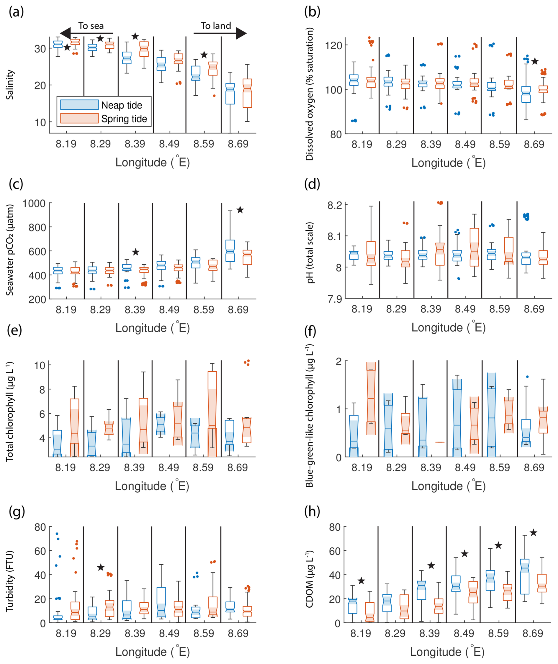
Figure 5 Box plots of salinity (a), dissolved oxygen saturation (b), seawater pCO₂ (c), pH (d), total chlorophyll concentration (e), blue-green-like chlorophyll concentration (f), turbidity (g), and CDOM (h) grouped in six regions in the outer Elbe Estuary, comparing the neap (blue) and spring (red) tide measurements. The box plots display the median, interquartile range, and outliers. When the notches of two box plots do not overlap, they have different medians at the 5 % significance level. Statistically significant differences between spring and neap tide groups according to a Welch t test are indicated using star symbols.

Figure 6 presents data from the same period as that shown in Fig. 4 but for the outer Elbe Estuary. The tidal range is again shown on a secondary axis, but this time the axis is reversed so that spring tide events are represented by the curve moving away from the river end on the right side of the diagram. The tidal range, usually between 3.25 and 4.25 m, was smaller than in the Humber Estuary. Here, typical conditions that coincided with the peak spring tide in the Humber Estuary – low salinity, oxygen undersaturation, high pCO₂, high chlorophyll, and high turbidity – occurred with a delay after the spring tide (peaks in colour changes in Fig. 6 happen after the apexes in the tidal range line). This time lag was between 4–5 d, when the tidal range was dropping and the system was close to entering a neap tide stage. Blue-green algae (Fig. 6f) were not a major contributor to the total chlorophyll concentration (Fig. 6e) in the Elbe Estuary. Maximum turbidity (Fig. 6g) and CDOM (Fig. 6h) were lower and higher than in the Humber Estuary, respectively (Fig. 4g and h).

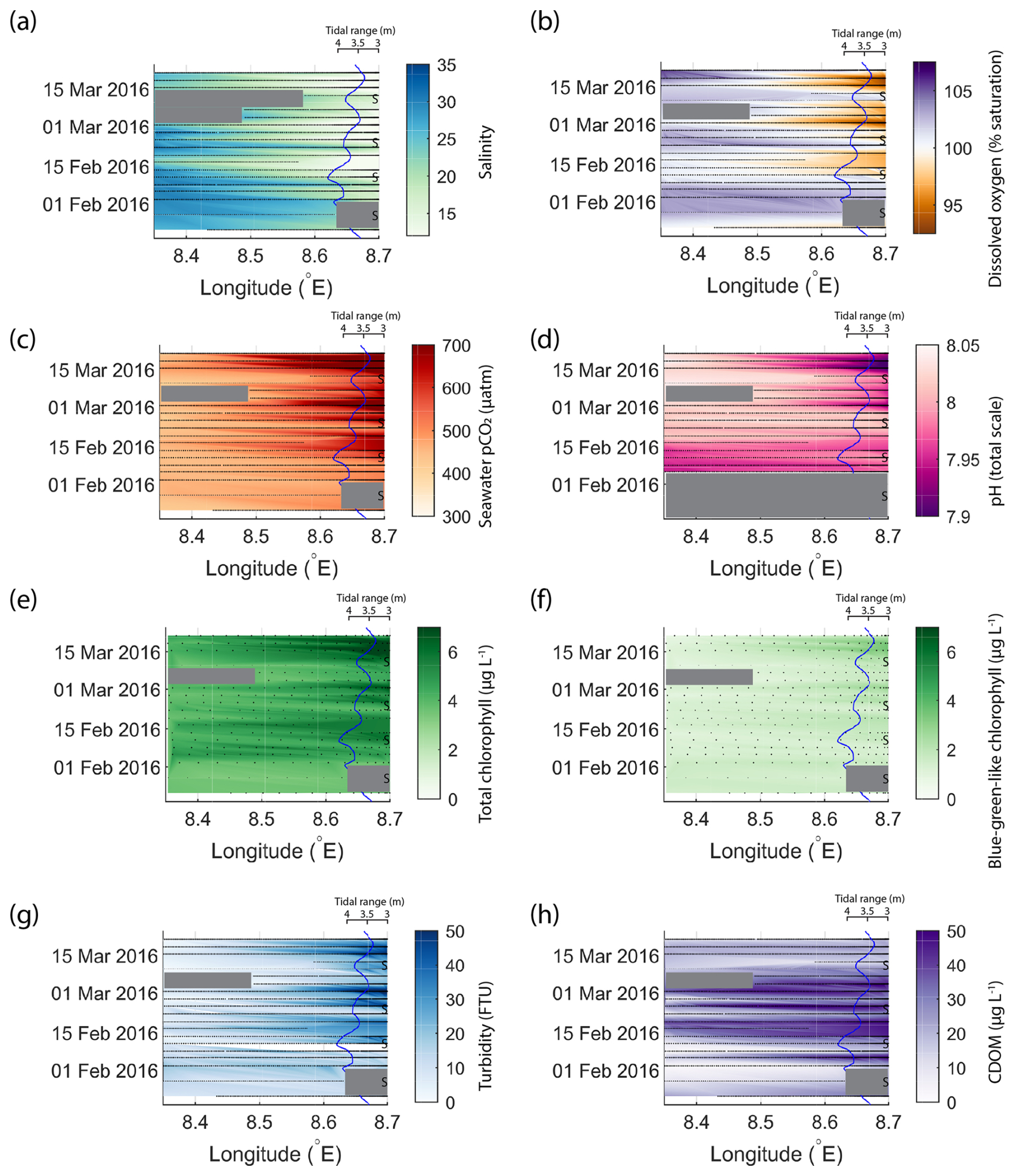
Figure 6 Variability in biogeochemical parameters in the outer Elbe Estuary during the same period as shown for the Humber Estuary in Fig. 4. The time and longitude coordinates of the measurements are shown in black. The tidal range is shown using the blue line, and spring tides are indicated using “S”. Note the reversal of the axis and the change in tidal amplitude compared to Fig. 4. Large data gaps are masked out with grey boxes. The variables shown are salinity (a), dissolved oxygen saturation (b), pCO₂ (c), pH (d), total chlorophyll (e), blue-green-like chlorophyll (f), turbidity (g), and CDOM (h).

3.3 Comparing the Humber and Elbe outer estuaries

There are differences identified in the previous sections; therefore, in Table 2, we provide a comparative summary of some correlations between the measured biogeochemical parameters in each outer estuary, and we also present the relative phytoplankton algal class composition.

Table 2 Comparison of the respective Pearson correlation coefficients of seawater salinity and pCO₂ with other FerryBox-measured essential ocean variables (EOVs). Data from the whole 3-year time series divided between the two studied estuaries are used, irrespective of tidal cycle. All correlation coefficients are significant at the 0.01 level, and the number of measurements for each correlation is indicated. Also shown is the relative contribution of plankton species in the two outer estuaries. The total chlorophyll-a concentration is split into these four constituents.

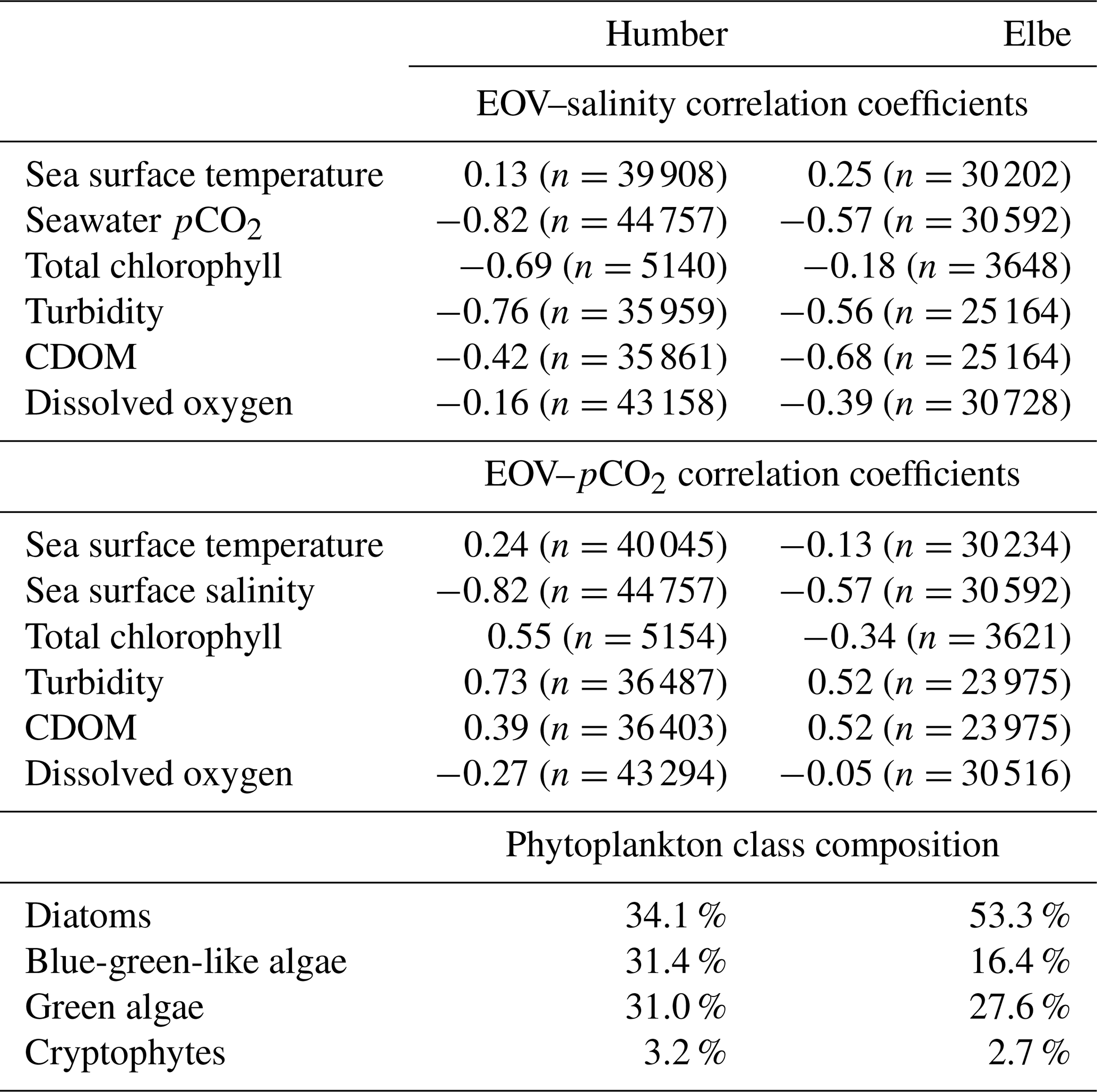
The negative correlation coefficients between salinity and pCO₂, chlorophyll, turbidity, CDOM, and oxygen suggest that all of these parameters are higher in the low-salinity endmember. Turbidity, CDOM, and pCO₂ are all higher in the low-salinity endmember than in the shelf sea and are, therefore, positively correlated with each other in this estuarine setting. The relative contribution of blue-green-like algae was higher in the outer Humber Estuary than in the outer Elbe Estuary, where diatoms produced more than half of the observed phytoplankton chlorophyll.

3.4 Spring–neap effects on sea–air carbon fluxes at the land–sea interface

The seawater pCO₂ in the outer Humber Estuary was higher than the atmospheric level, indicating that this estuarine outflow on the coast is a potential carbon source to the atmosphere. Moreover, the seawater pCO₂ was much higher during spring tides (Figs. 3c and 4c) than during neap tides (increasing from a mean of 640 ± 59 to 813 ± 142 µatm at the most upstream location), leading to the estuary becoming a stronger potential source of carbon dioxide to the atmosphere, which we calculate here. If this spring–neap cycle difference is not considered, assessments of the role of estuaries in regional carbon budgets might underestimate the contribution of estuaries to the carbon cycle. We calculate average seawater pCO₂ at the same locations as the box plot analysis (Fig. 3c) and use these averages and the average 2015–2017 atmospheric pCO₂ (401 ± 6.2 µatm) to calculate sea–air carbon dioxide fluxes at each location and differentiate between the CO₂ flux during neap and spring tides. We found no correlation between the daily averaged wind speed data and the tidal amplitude (Pearson's p value of 0.45, tested on 181 data points in the first 6 months of 2017). As there was no association between the higher pCO₂ at spring tides with, for example, higher wind speeds, we use the climatological average of the ERA5 wind speed in the Humber Estuary of 6.9 m s⁻¹. This isolates the investigated influence on sea–air carbon fluxes to tidally driven seawater pCO₂ (and not to wind speed). We calculate CO₂ fluxes using the “CO2flux” function available online (https://github.com/mvdh7/co2flux, last access: 26 March 2025) (Humphreys et al., 2018) with the Wanninkhof (2014) gas transfer parameterization and the Weiss (1974) carbon dioxide solubility. At 0.4° E, where the riverine influence is limited, the average neap flux was 3.6 ±3.7 mmol C m⁻² d⁻¹ and the average spring flux was 5.0 ±5.5 mmol C m⁻² d⁻¹. At the most upstream location, the increase between neap and spring tide averages was around 74 %, from 24.7 ±7.9 to 43.0 ± 17.1 mmol C m⁻² d⁻¹, respectively. The uncertainties in the flux calculations are propagated using the uncertainty of the atmospheric pCO₂, the standard deviation of the mean of the seawater pCO₂ measurements at a certain location and tidal category, and the 20 % uncertainty for the gas transfer velocity coefficient found by Wanninkhof (2014). Monthly averaged climatological wind speeds at our studied location range from 5.3 to 8.4 m s⁻¹, but we only use the annual average because our observations span multiple years and we do not differentiate by month. We defined an area the width of the river channel upstream and the width of the observational coverage offshore and integrated the fluxes over the resulting boxes. Based on our definition of spring and neap tide periods, these occupy around 50 d in 1 year. Therefore, based on the 2015–2017 conditions, the outer Humber Estuary releases 2.1 ± 1.2 Gg C yr⁻¹ to the atmosphere during neap tide periods, compared to 3.4 ± 2.1 Gg C yr⁻¹ during spring tide periods, changing the area-integrated sea–air flux of this estuary during spring tide by over 60 %. This change does not refer to the rest of the 265 d during transitional tidal periods.

4 Discussion

4.1 Drivers of biogeochemical variability

The spring–neap tidal cycles influence the strength of the potential carbon source to the atmosphere in outer estuaries, accounting for the largest variability in pCO₂ on timescales longer than semi-diurnal, based on Fourier transform analysis (Fig. 2c). In outer estuaries like the Humber Estuary, this results in a stronger (by over 60 %) area-integrated carbon source to the atmosphere during spring tides compared to neap tide conditions. In our observations, the periodicity of the biogeochemical changes, including salinity, turbidity, seawater pCO₂, dissolved oxygen saturation, and chlorophyll, largely aligns with the spring–neap tidal cycle periodicity, suggesting that this is an essential modulator of carbon cycling and ecosystem parameters at the land–sea interface. Below, we identified the processes that likely force the outer Humber Estuary system to experience the observed spring–neap pCO₂ tidal variability.

Estuaries are generally considered to be net heterotrophic environments and sources of carbon to the atmosphere (Smith and Hollibaugh, 1993; Chen and Borges, 2009; Cai, 2010; Canuel and Hardison, 2016; Volta et al., 2016). In contrast, shelf seas, such as the North Sea, are generally net autotrophic, and their in situ primary production is driven by the riverine nutrient loads (Kühn et al., 2010). Therefore, the outer-estuary region is characterized by large gradients, with respect to not only salinity but also biogeochemical parameters, such as nutrient concentrations and pH (Kerimoglu et al., 2018). The observed spring tide oxygen undersaturation and increase in seawater pCO₂ in the outer Humber Estuary are indicative of a net heterotrophic environment. While higher chlorophyll concentrations were also observed during spring tides, we postulate that this is not locally produced biomass and does not lead to a decrease in seawater pCO₂ via autochthonous primary production. Water mass movement simulations (Fig. S4) suggest that the chlorophyll observed in the outer estuary during spring tides could be allochthonous and could be produced in the river or inner estuary. The similarity of the observed chlorophyll fluorescence to blue-green-algae-like material also hints towards a more inland origin of the organic matter. The cells could be damaged in contact with salt water, and the chlorophyll released can be observed by our instruments (Yang et al., 2020). The Humber Estuary is generally turbid and exhibits an increase of at least 18 % in turbidity during spring tides. These conditions do not facilitate local primary production that would lower the seawater pCO₂.

4.2 Organic matter transformations at the estuary–sea interface

In the outer estuaries of Humber and Elbe, the negative correlation between CDOM and salinity and the positive correlation between CDOM and pCO₂ (Table 2) confirm our existing knowledge about the origin and estuarine distribution of this component of the riverine dissolved matter. For instance, CDOM was strongly negatively correlated with salinity and showed a conservative behaviour indicative of a terrestrial source in a study of Norwegian rivers (Frigstad et al., 2020). Dissolved organic carbon, for which CDOM can be used as a proxy, can feature a variety of behaviours in estuaries depending on the flushing time and variations in the source of organic matter (Bowers and Brett, 2008; García-Martín et al., 2021). What is particularly noteworthy in our study is that higher CDOM concentrations were usually associated with neap tides in both estuaries (Figs. 3h and 5h). This suggests that the fraction of organic carbon in the dissolved form in the outer estuary is larger during the neap tide periods than during spring tides. At the same time, inorganic carbon in the form of dissolved carbon dioxide also varies with the spring–neap cycle (Figs. 3c and 5c). This has an impact on the quantity and type of lateral carbon transport across the LSI. On a shorter timescale of variability, Chen et al. (2016) found examples of higher CDOM during the ebb tide phase, when phytoplankton is not dispersed by the more dynamic conditions at high tide. The resuspension of bottom sediments at spring tide might also suppress the effect of terrestrial sources, usually the main input of CDOM to the estuary (Ferreira et al., 2014). High CDOM can also come from the bacterial degradation of phytoplankton-derived detritus (Astoreca et al., 2009), and high turbidity can protect the detritus from photodegradation (Juhls et al., 2019), although the switch between tidal conditions might be too fast for this process to play a major role. We postulate that, in tidally driven outer estuaries, cycling between the spring and neap tidal stages provides favourable conditions for dissolved organic material to be either brought to the surface from the benthos or transported to the outer estuary from further inshore during spring tides and subsequently transformed into a measurable form during neap tides by our CDOM instrument.

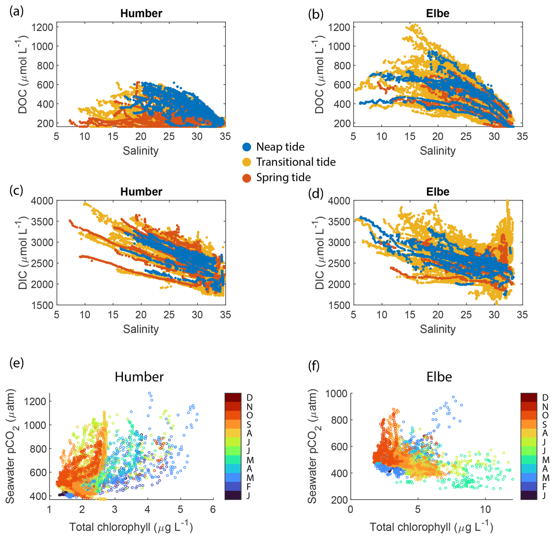
Figure 7 Estimated (a, b) dissolved organic carbon and (c, d) dissolved inorganic carbon concentrations in the Humber and Elbe estuaries plotted against salinity and colour-coded according to the spring–neap tidal cycle. The relationship between seawater pCO₂ and total chlorophyll in the outer estuaries of the (e) Humber and the (f) Elbe. The data points are colour-coded by month.

The addition of dissolved organic matter in the outer estuary is supported by the positive non-linear distribution of CDOM-derived DOC against a theoretical linear salinity gradient when assuming conservative mixing (Fig. 7a, b), indicating a source of DOC within the estuary, at the LSI. Although we do not capture salinities for the freshwater endmember, some data points in the middle of the outer estuary lie above the line connecting the marine term to the lowest available salinity. The DOC enhancement at intermediate salinity values was pronounced during neap tides in the Humber; for example, at salinities of 22.5 ± 1, the mean spring tide DOC concentration was 297 ± 106 µmol L⁻¹, while the mean neap tide DOC was 467 ± 86 µmol L⁻¹. There was no similar pattern in the Elbe, where the mean DOC concentrations were higher than in the Humber example at the same salinity values but were statistically indistinguishable between spring and neap tide. The ratio between the forms of dissolved carbon favoured the inorganic one. At a salinity of 20 ± 1, DOC was approximately 10 % and 18 % of the total dissolved carbon pool in the Humber and the Elbe, respectively. This is slightly lower than the 20 % average in UK rivers (Jarvie et al., 2017). The calculated DOC concentrations for the outer Humber Estuary were higher than the Humber riverine endmember used by García-Martín et al. (2021), in the range reported by Tipping et al. (1997) for the Humber and by Williamson et al. (2023) for the Trent tributary, and actually lower than the Humber value reported by Painter et al. (2018) and Dai et al. (2012). The Elbe DOC concentrations were within the range of measurements conducted by the Flussgebietsgemeinschaft Elbe at the Cuxhaven station (FGG Elbe-Datenportal, River Basin Community; https://www.fgg-elbe.de/elbe-datenportal.html, last access: 26 March 2025). The linear empirical DOC:CDOM relationship that we used has a high intercept of 162 µmol L⁻¹. This means that there is DOC in the water even when the CDOM fluorescence readings are zero. The fluorometer can only detect a specific fluorescent chemical group and nothing that does not fluoresce. Furthermore, in a study in the coastal Arctic, another empirical relationship between DOC and CDOM quinine sulfate fluorescence found a similarly high intercept of 110 µmol L⁻¹ (Pugach et al., 2018). Mid-estuary non-conservative DOC enhancement, such as in our study, was also found by McKenna (2004), who attributed it to phytoplankton-derived autochthonous inputs. In the studied estuaries, the measured high chlorophyll concentrations coincide with low oxygen; hence, the primary production happens elsewhere, and the DOC that we observe at neap tides is a result of transformations of allochthonous organic matter. Alternatively, the high turbidity during spring tides could prevent our fluorescence-based instrument from detecting the entire amount of CDOM present in the surface waters.

The calculated DIC on the Elbe side was higher than other reported values in the Elbe Estuary or German Bight (Reimer et al., 1999; Rewrie et al., 2023b), but similar relationships with salinity in the outer Elbe Estuary were observed at certain times during our period of observations, as shown in the Supplement provided by Rewrie et al. (2023b). The DIC values reported here are, however, subject to the combined uncertainties in the measurements and the calculations. The pCO₂–pH pair, which we used due to our data availability, has the highest calculation uncertainty, with a carbonate ion squared combined standard uncertainty of nearly 40 µmol kg⁻¹ (Orr et al., 2018). There were also DIC data in the Elbe outflow at salinities higher than 30 which did not follow the salinity relationship of the other data points (Fig. 7d). These data were calculated using measurements from July–August 2017, a period during which another study found elevated DIC concentrations in the Elbe Estuary (Rewrie et al., 2023a).

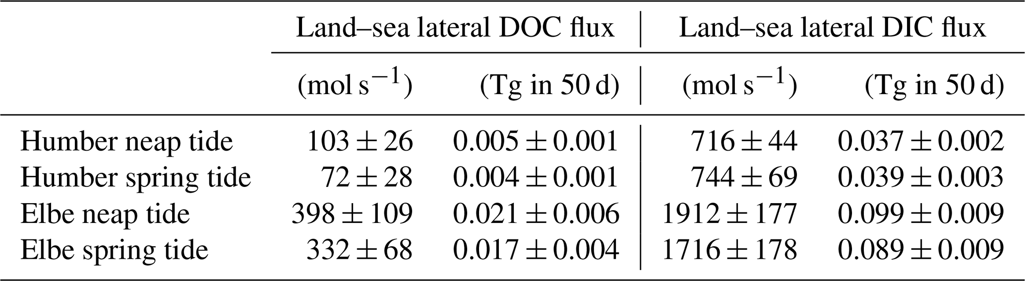
Having observed the spring–neap influence on the concentrations of dissolved carbon fractions, we used the average DOC and DIC concentrations at the most upstream locations sampled (westernmost longitude group in the outer Humber Estuary box plot and easternmost longitude group in the outer Elbe Estuary) to provide a quantitative assessment of lateral land–sea fluxes (Table 3). We use average literature discharge for the Humber and the 2016–2017 measured discharge for the Elbe (FGG) adjusted for tributary influence based on Amann et al. (2012). We also employ a similar methodology to the vertical carbon flux calculations in Sect. 3.4 to calculate the mass of carbon transported during the spring or neap tide events in an average year, excluding the other 265 d during transitional tide periods. The lateral flux of DOC is 43 % and 20 % higher during neap tide in the Humber and Elbe outer estuaries, respectively. The lateral flux of DIC in the Elbe also increases by 11 % during neap tides, whereas the DIC flux decreases by 4 % during neap tides in the Humber. All of the differences are statistically significant at the 5 % level, tested with a two-sample t test. We also provide the equivalent mass transport out of our estuaries during the two different tide events. For context, Kitidis et al. (2019) estimate a whole Northwest European Shelf DOC and DIC riverine flux of 2.1 and 18.9 Tg C yr⁻¹, respectively, upstream of the estuaries and 2.6 and 2.0 Tg C yr⁻¹, respectively, in the outer estuaries.

Table 3 Average (± standard deviation) lateral organic and inorganic carbon fluxes from the two outer estuaries depending on the spring–neap tidal stage.

There are also differences between the two outer estuaries related to the dissolved oxygen and chlorophyll measurements. In an open-marine setting, oxygen and pCO₂ are strongly inversely correlated, which is a function of primary production and respiration (DeGrandpre et al., 1997). In coastal regions, however, there are distinct pCO₂-to-dissolved oxygen relationships due to variability in Revelle factors and different sea–air equilibration times (Zhai et al., 2009). In both the Humber and Elbe outer estuaries, pCO₂ and dissolved oxygen were inversely correlated, although the correlation was weak in the Elbe. Combining this with the direct versus inverse correlations between pCO₂ and chlorophyll in the Humber and Elbe, respectively (Table 2), indicates that the two outer estuaries have a different metabolic behaviour. Having high chlorophyll coinciding with low oxygen and high pCO₂ suggests that the chlorophyll was not locally produced in the outer Humber Estuary. Instead, this location is the site where chlorophyll-containing organic matter that was likely produced upstream in the estuary was typically remineralized. During the summer and autumn seasons, however, in months when the minimum seawater temperature was higher than 12.5 °C, the relationship was closer to what is expected during conventional marine primary production (orange tones at pCO₂ levels below 550 µatm in Fig. 7e). When combining the whole-year data and including the very high pCO₂ brackish-water-influenced measurements, the usual negative correlation changes. Due to the location of the ports, the ship did not enter the Elbe Estuary main channel as far upstream as in the Humber Estuary (Fig. 1d and c, respectively); therefore, in the outer Elbe Estuary, we were observing a more typical marine behaviour (Fig. 7f). The outer Humber Estuary is highly turbid and a location of organic matter degradation, whereas the organic matter in the Elbe is processed further upstream in the estuary, allowing the outer Elbe Estuary to take up some carbon through organic matter production, leading to the differences in Fig. 7e and f.

Some studies have found that higher chlorophyll concentrations in estuaries are associated with neap tides, when the water residence time is longer and conditions are calmer (Lucas et al., 1999; Trigueros and Orive, 2000; Domingues et al., 2010; Flores-Melo et al., 2018). Production from phytoplankton is limited by light and nutrient availability. In estuarine settings, the high nutrient availability means that the chlorophyll peak usually coincides with peak solar irradiance (Jakobsen and Markager, 2016). Over a longer seasonal term, this guides the onset of spring plankton blooms. On shorter timescales, the optimal conditions for primary production occur at the onset of stratification, as the estuary is shifting towards a neap tide stage but also benefiting from the extra nutrients brought to the surface during the previous dynamic spring tide stage. This succession of events is what likely led to our outer Elbe Estuary observations (Fig. 6e). In contrast to the paradigm of high chlorophyll at neap tides and similar to what we observed in the Humber Estuary, the Tagus estuary in Portugal showed higher biomass during spring tides (Cereja et al., 2021). This was caused by the resuspension of sediments and the mixing of microphytobenthos into the water column, a phenomenon also described by Macintyre and Cullen (1996). The high chlorophyll concentrations that we measured during spring tide in the Humber Estuary either have a similar origin or, alternatively, come from somewhere else and are, therefore, not locally produced.

The dominant phytoplankton class were diatoms, while green algae made up around 30 % of the total chlorophyll in both estuaries. However, the relative abundance of blue-green-like algae in the Humber was nearly double that in the Elbe (31 % versus 16 %, respectively; Table 2). This was mainly driven by the increasing blue-green-like-algae chlorophyll concentrations at spring tides (Figs. 3f and 4f). Blue-green algae, or cyanobacteria, are microscopic photosynthetic prokaryotes, which are more common in freshwater (Iriarte and Purdie, 1993). Their occurrence in the North Sea is usually restricted to the Skagerrak–Norwegian Channel region (Brandsma et al., 2013). Although this study focuses on estuary-influenced regions, and cyanobacteria can actually dominate the plankton biomass in estuaries or be in phase with tidally driven stratification events (Eldridge and Sieracki, 1993; Murrell and Lores, 2004), there are likely no relevant concentrations of cyanobacteria in this region of the North Sea. The instrument is possibly interpreting the fluorescence excitation from a slightly different algal group as that coming from cyanobacteria. During an usual open-ocean spring bloom, the most efficient nutrient-utilizing plankton are the diatoms (Flores-Melo et al., 2018). What we could be observing in the outer Humber Estuary is a smaller-scale version of this effect, where diatoms are outcompeting other algae during neap tides, and the latter are utilizing the spring tide niche for their development (Rocha et al., 2002). Alternatively, if the chlorophyll that we observed at spring tides was not autochthonous, our observations could be influenced by how refractory the material is. Different phytoplankton species release varying dissolved organic matter, and the organic matter from the blue-green-like algae is more resistant to degradation by microorganisms and, therefore, observable by our instruments (Osterholz et al., 2021).

4.3 Models versus observations

The carbon flux to the atmosphere in the outer Humber Estuary ranged between 3.6 mmol m⁻² d⁻¹ offshore at neap tide and 43.0 mmol m⁻² d⁻¹ nearshore at Immingham at spring tide. This places the outer-estuary outgassing between estimates for the southern North Sea at 2.1 mmol m⁻² d⁻¹ (Prowe et al., 2009) and Northwest European Shelf estuaries as a whole at 54–170 mmol m⁻² d⁻¹ (Kitidis et al., 2019), but it emphasizes the proper accounting of this flux with consideration of the spring–neap cycle. Excess dissolved inorganic carbon produced by respiration and remineralization makes estuaries carbon sources to the atmosphere. A study found that about 60 % of the heterotrophic carbon in an estuary was lost by evasion to the atmosphere (Raymond et al., 2000). Here, we show that this evasion happens along a gradient and varies according to the different stages in the tidal spring–neap cycle; therefore, the estuarine influence on nearshore seawater pCO₂ can extend further offshore than expected, depending on a reference point, with influence on regional flux calculations.

The importance of the LSI is now a more prominent topic in the literature, and the knowledge gaps are identified as research priorities (Legge et al., 2020). The areas adjacent to river mouths were necessary to consider when closing the carbon budget of the Baltic Sea (Kuliński and Pempkowiak, 2011). We have evidence that high-pCO₂ waters can be advected seaward due to river outflow and tidal exchanges (Reimer et al., 2017). The Southern Bight of the North Sea was a carbon sink over an annual integration with a flux of 2.27 mmol m⁻² d⁻¹, but including estuarine plumes in the calculation decreased the carbon uptake potential to 1.78 mmol m⁻² d⁻¹ (Schiettecatte et al., 2007). In spite of all this, some Earth system models still lack the implementation of estuarine systems because of the computational constrains with respect to reproducing their variability (Regnier et al., 2013). We observed this effect in particular for the outer Humber Estuary region in a previous study (Macovei et al., 2022). A model that correctly replicated high chlorophyll observations in the central North Sea also replicated the associated decrease in sea surface pCO₂. However, the same model underestimated seawater pCO₂ in the area of influence of the Humber Estuary, likely because it associated the high chlorophyll recorded during spring tides with carbon dioxide drawdown. Here, we show that these variables are not necessarily negatively correlated in outer estuaries (Fig. 7e, Table 2), where conflicting processes occur, and this can lead to incorrect CO₂ sea–air flux estimates. As for all coastal environments, outer estuaries are also vulnerable to anthropogenically driven climate change, and uncertainty regarding the direction of change remains. Resolving the competing and rapidly varying processes of the future river-influenced coastal seas first requires a thorough understanding of the present-day processes.

5 Conclusion

Estuaries are complex environments, with tides inducing large variability in biogeochemical parameters. Here, we used the high measurement frequency and multitude of sensors that FerryBox systems installed on a ship of opportunity allow and described the spring–neap tidal variability in two large outer estuaries draining into the North Sea. We find that spring–neap variability plays an important role in modulating carbon fluxes at the land–ocean interface. Moreover, this study demonstrates that the spring–neap variability usually seen at a fixed-point station can also be observed from a regularly transiting ship, with the added benefit of determining the spatial extent of the estuarine influence on the coast. In the macrotidal, well-mixed Humber Estuary, seawater pCO₂ was up to 21 % higher during the more turbid spring tides, under heterotrophic conditions, as shown by the widespread oxygen undersaturation. At the most upstream location in our study area in the outer Humber Estuary, the sea-to-air carbon dioxide flux increased from 24.7 ± 7.9 mmol C m⁻² d⁻¹ during neap tides to 43.0 ± 17.1 mmol C m⁻² d⁻¹ during spring tides. The lateral dissolved organic carbon flux, on the other hand, increased from 72 ± 28 mol s⁻¹ during spring tides to 103 ± 26 mol s⁻¹ during neap tides. This means that the strength of carbon evasion from macrotidal, well-mixed estuaries could be misrepresented in models and budget calculations if the fortnightly tidal cycle is not considered. Moreover, we showed that the estuarine outflow influence stretched at least 7 km offshore and that this is sometimes not correctly reproduced in models, as observed by Macovei et al. (2022) using another dataset. We described the competing processes forcing pCO₂ in the outer estuaries and showed how different biogeochemical parameters correlate. Spring tide conditions were associated with higher phytoplankton biomass, mainly driven by blue-green-like algae, which were remineralized in the outer estuary. Neap tide conditions were associated with higher CDOM, produced in the estuary, likely derived from allochthonous material. The dissolved carbon pool in both outer estuaries studied here was dominated by the inorganic form, with DOC being less than 20 % of the total. However, indications of the non-conservative addition of DOC into the outer estuary were observed at intermediate salinity values, in particular in the Humber, where DOC concentrations during neap tides were 57 % higher than during spring tide, altering the lateral flux ratio of dissolved organic to dissolved inorganic carbon across the LSI depending on the spring–neap cycle. The conclusions presented describe well-mixed tidal outer estuaries, and this is an important first step in understanding the drivers of biogeochemical variability in classical estuaries before the complexity of global-scale land–sea interactions are assessed. Although the North Sea is one of the most studied marginal seas, its biogeochemistry is still not fully parameterized for integration into models, in particular in the freshwater-influenced areas. With this study, we are following the call of the community by providing observations at the land–ocean interface, and our results can be used to improve the performance of regional biogeochemical models, with ulterior upscaling into Earth system models and carbon budgeting.