Disentangling future effects of climate change and forest disturbance on vegetation composition and land surface properties of the boreal forest

Forest disturbances can cause shifts in boreal vegetation cover from predominantly evergreen to deciduous trees or non-forest dominance. This, in turn, impacts land surface properties and, potentially, regional climate. Accurately considering such shifts in future projections of vegetation dynamics under climate change is crucial but hindered (e.g., uncertainties in future disturbance regimes). In this study, we investigate how sensitive future projections of boreal forest dynamics are to additional changes in disturbance regimes. We use the dynamic vegetation model LPJ-GUESS to investigate and disentangle the impacts of climate change and intensifying disturbance regimes in future projections of boreal vegetation cover as well as changes in land surface properties such as albedo and evapotranspiration. Our simulations find that (1) warming alone drives shifts towards more densely forested landscapes, (2) more intense disturbances reduce tree cover in favor of shrubs and grasses, and (3) the interaction between climate and disturbances leads to an expansion of deciduous trees. Our results additionally indicate that warming decreases albedo and increases evapotranspiration, while more intense disturbances have the opposite effect, potentially offsetting climate impacts. Warming and disturbances are thus comparably important agents of change in boreal forests. Our findings highlight future disturbance regimes as a key source of model uncertainty and underscore the necessity of accounting for disturbances-induced effects on vegetation composition and land surface–atmosphere feedback.

1 Introduction

Climate change induces widespread changes in ecosystem state and functions (McDowell et al., 2020; Allen et al., 2010). Next to changing mean conditions, climate change is expected to lead to an increase in extreme climatic events in many regions (Calvin et al., 2023; Field, 2012; Rahmstorf and Coumou, 2011). At the ecosystem level, this alters regimes of ecosystem disturbances such as fire, windthrow, or biotic agents (McDowell et al., 2020; Seidl et al., 2017; Reichstein et al., 2013).

Such disturbances may lead to widespread tree mortality and loss of forest cover. While they are inherent elements of many forest ecosystems, changes in disturbance regimes (i.e., changes in their frequency, intensity, or size) can nevertheless have profound impacts, especially in systems already subjected to environmental pressure, where resilience and regeneration abilities are low (Pugh et al., 2019a; Allen et al., 2010; Johnstone et al., 2016). Understanding the impact of disturbances is, therefore, crucial for reliably projecting the future development of forest ecosystems under climate change.

The boreal forest, or taiga, is the second-largest terrestrial biome with respect to both area and carbon mass (Pan et al., 2024, 2011; Malhi et al., 1999), spanning the Northern Hemisphere in a circumpolar band between approximately 50 and 70° N. (Pfadenhauer and Klötzli, 2020). Its characteristic vegetation comprises conifer forests, dominated by various species of Abies, Picea, and Pinus in North America and western Eurasia and by Larix in Siberia (Pfadenhauer and Klötzli, 2020). In the boreal forest, disturbances are an integral part of ecosystem dynamics, and tree species are thus adapted and resilient to historical disturbance regimes (Pfadenhauer and Klötzli, 2020; Ilisson and Chen, 2009; Johnstone et al., 2010). However, evidence from both paleoecology (Peros et al., 2008; Edwards et al., 2005) and recent field surveys (Baltzer et al., 2021; Mack et al., 2021; Johnstone et al., 2010; Brice et al., 2020) suggests that changing disturbance regimes can disrupt existing successional cycles and induce reorganization of the complete ecosystem. In many places, evergreen needleleaf trees fail to regenerate after disturbance, and transitions to broadleaf summergreen forests or non-forest ecosystems are reported (Baltzer et al., 2021; Mack et al., 2021).

Boreal forests influence regional and global climate (Bonan, 2008; Randerson et al., 2006). Aside from being a carbon sink, vegetation composition influences surface properties such as albedo or evapotranspiration. (Swann et al., 2010; Liu et al., 2019; Rogers et al., 2013; Bonan, 2008; Chapin et al., 2005). Shifts in vegetation composition can, therefore, result in significant alterations to the carbon, water, and energy balance of the region (Mack et al., 2021; Boisier et al., 2013; Zhang et al., 2013; Alexander et al., 2012; Swann et al., 2010; Bonan, 2008). Consequently, understanding the role of disturbance-induced vegetation shifts in future vegetation and climate dynamics and their accurate representation in climate change projections are important.

Several studies have tackled part of this question; for example, Kim et al. (2024), Wang et al. (2020), and Sulla-Menashe et al. (2018) aimed to quantify the disturbance effect from observations. However, this remains incomplete, as disturbed sites are also subject to background climate change, and the disturbance effect can therefore not be isolated. Additionally, observational time series of forest dynamics, especially large-scale assessments from remote sensing, are still relatively short (∼ 30 years) compared to the multidecadal to centennial timescales of forest succession. While longer time series of post-disturbance dynamics can be constructed from chronosequences, those rely on a space-for-time substitution effect and do not take temporal changes in climate into account. Therefore, it remains difficult to pinpoint if the observed changes will be permanent or transient in nature.

Process-based vegetation models are a prime research tool to complement observational findings in these regards, as they allow for the factorial simulation of different drivers over longer time periods. Zhang et al. (2020), Wårlind et al. (2014), Zhang et al. (2013), Warszawski et al. (2013), Foster et al. (2019), and Wolf et al. (2008) explored the impact of future climate change on boreal forest dynamics and land surface properties with dynamic vegetation models (DVMs) without considering changes in disturbance regimes. Rogers et al. (2013) investigated the impact of changing disturbance regimes on land surface properties and climate but did not consider climate change effects on vegetation. Hansen et al. (2021), Brice et al. (2020), Foster et al. (2022), and Mekonnen et al. (2019) explored the interplay between climate change and disturbance regimes for parts of Alaska and Canada over the 21st century. However, none of these studies explored long-term effects beyond the 21st century or regeneration after disturbance. To our knowledge, no biome-wide modeling studies currently exist that systematically investigate both 21st-century and long-term future impacts of changing disturbance regimes, climate change, and their interaction for different climate futures.

In this study, we use the DVM LPJ-GUESS (Smith et al., 2001, 2014) to fill this gap. LPJ-GUESS includes a process-based representation of plant physiology (photosynthesis, respiration, and evapotranspiration) and resolves the vegetation structure at the level of individual tree cohorts, organized into multiple patches across the landscape. This allows for the simulation of disturbances, mortality, and establishment in a way well suited to the study of disturbance regimes and post-disturbance regeneration. We perform factorial simulation experiments of both different climate scenarios and external disturbance regimes, spanning return intervals from the low end of what is historically observed to the high end of what is historically observed and projected for the future, to disentangle their respective future roles in vegetation dynamics of high-latitude forests.

We address the following research questions:

1. What is the impact of climate change, changing disturbance regimes, and their interactive effect on boreal vegetation composition?

2. How do changes in vegetation influence climate-relevant biogeophysical land surface properties, namely, albedo and evapotranspiration?

3. Are disturbance-induced changes permanent or is vegetation able to regenerate once disturbance pressure is again lifted?

2 Methods

2.1 Vegetation modeling

2.1.1 General LPJ-GUESS model description

We work with version 4.1 of the well-established dynamic vegetation model LPJ-GUESS (Smith et al., 2001, 2014; Nord et al., 2021), driven by gridded temperature, precipitation, and downwelling shortwave radiation, as well as global CO₂ concentrations and soil properties. Here, we use a version parameterized for Arctic vegetation, as summarized in Table A1. This version has been validated in previous studies, e.g., against species distribution maps (Zhang et al., 2013; Miller and Smith, 2012; Wolf et al., 2008), flux measurements of carbon cycle dynamics (Rawlins et al., 2015; McGuire et al., 2012), observational data of snowpack and soil properties (Pongracz et al., 2021; Chaudhary et al., 2020), and remotely sensed land surface properties (Zhang et al., 2018).

Plant physiological processes follow the approach of LPJ-DGVM (Sitch et al., 2003). As the focus of this study is on vegetation dynamics, we briefly sketch out the main processes here – as described in detail by Smith et al. (2001) and Smith et al. (2014) – followed by a detailed description of population dynamics and disturbances. CO₂ and water fluxes are calculated by a coupled photosynthesis and stomatal conductance scheme based on the approach of BIOME3 (Haxeltine and Prentice, 1996). For each simulation year, the net primary production (NPP) accrued by an average individual plant is allocated to leaves, fine roots, and (for woody plants) sapwood, following a set of prescribed allometric relationships (Sitch et al., 2003). Litter from phenological turnover, mortality, and disturbances enters the soil decomposition cycle. For details on soil processes, including C–N dynamics and soil hydrology, refer to Smith et al. (2014), Sitch et al. (2003), and Gerten et al. (2004).

2.1.2 Population and disturbance dynamics in LPJ-GUESS

LPJ-GUESS employs a hierarchical model structure that allows for a detailed representation of population dynamics such as recruitment, competition, and disturbance. Within each grid cell of climate data (0.5°×0.5° resolution), multiple patches are simulated (25 patches are used in this study). Patches can be thought of as a random, independent sample of the grid cell; thus, the model outputs the average across all patches in a grid cell. Vegetation dynamics within each patch emerge from growth and competition for light, space, and soil resources among woody-plant cohorts and a herbaceous understory. Plants within a patch are represented by different age cohorts of a number of plant functional types (PFTs) described by properties such as growth form, phenology, photosynthetic pathway (C₃ or C₄), and bioclimatic limits (see Table A2 for the PFT parameterization used in this study). Each age cohort includes multiple individuals of that PFT assumed to all have identical properties (“cohort mode”). Establishment and mortality are represented as stochastic processes at the cohort level. Both the probability of establishment and disturbance depend on the productivity of the PFT. The probability of mortality additionally depends on the cohort age, whereas establishment depends on the amount of light reaching the forest floor. PFTs are able to reproduce as soon as they are productive.

Disturbances in LPJ-GUESS are equally modeled as a stochastic process. The expected frequency of disturbances is encoded through the yearly disturbance probability p_D. If a patch experiences a disturbance, aboveground vegetation is converted to coarse woody debris and slowly decomposes over time. Here, the patch structure emulates heterogeneity in the landscape and accounts for the fact that disturbances are not necessarily stand-replacing at the landscape scale. We opted for this standardized implementation of disturbances to reduce the degrees of freedom in our experiments and be able to focus on downstream impacts.

2.2 Input data

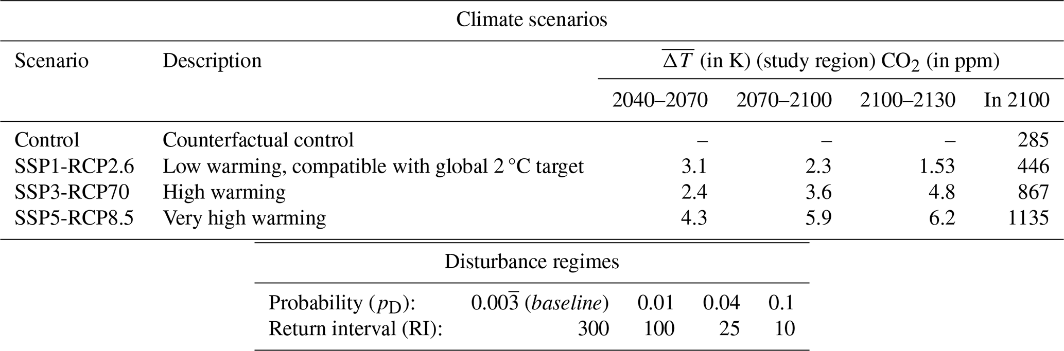
We run LPJ-GUESS with the daily simulated climate from the Inter-Sectoral Impact Model Intercomparison Project (ISIMIP) repository at a 0.5°×0.5° resolution (Lange and Büchner, 2021). From within the ISIMIP ensemble, data of the MRI-ESM2.0 Earth system model were chosen, as they feature a medium climate sensitivity and, thus, give a temperature response that best corresponds to the ensemble mean. We also use corresponding yearly atmospheric CO₂ concentration data from ISIMIP. We use all scenarios available from the ISIMIP – SSP1-RCP2.6, SSP3-RCP7.0, and SSP5-RCP8.5 – as well as a counterfactual Control scenario that was created with constant preindustrial CO₂ concentrations of 285 ppm but recreates non-CO₂ forcing and interannual variability (Fig. 1a and Table 1) Over the study region, both mean temperature and mean precipitation increase in all climate warming scenarios (Fig. A1). The climate response for the SSP3-RCP7.0 and SSP5-RCP8.5 scenarios is very similar, despite their different CO₂ levels. Temperature increases are most pronounced in the winter months (Fig. B1a). In the Control scenario, average temperatures remain below 0 °C from October to April, whereas this is the case from November until March in the strongest warming scenario SSP5-RCP8.5. Precipitation changes are stronger in the summer and also show higher interannual variability (Fig. B7b). We use soil data from the Harmonized World Soil Database, aggregated to the resolution of the climate data (FAO and IIASA, 2023). The model assumes yearly nitrogen deposition of 750 g ha⁻¹ (Tian et al., 2018).

2.3 Modeling protocol

We combined each climate warming scenario with a range of disturbance regimes. Equally, we combined all disturbance scenarios with a counterfactual Control climate simulation to account for interannual and decadal variability in climate. Thus, we simulated 16 scenarios in total (see Table 1 and Fig. 1b for an overview). To reduce dimensionality, for the purpose of this study, we describe disturbance regimes based on disturbance probability, while keeping intensity and size constant. We chose disturbance probabilities that span from the low end of what is historically observed (return intervals of ∼ 300 years; see, e.g., Burrell et al., 2022, and Rogers et al., 2013) to the high end of what is historically observed and projected for the future (return intervals up to 10 years; see, e.g., Buma et al., 2022, Burrell et al., 2022, or Turner et al., 2019).

We simulate all grid cells within the boreal forest (taiga) biome as being predominantly covered by needleleaf evergreen trees, as defined by the World Wildlife Fund (WWF) classification of terrestrial ecoregions of the world (Olson et al., 2001), after the spin-up period. We considered needleleaf evergreen trees to be dominant if that PFT constituted the maximum share of aboveground carbon (AGC) or fractional plant cover (FPC) in that grid cell. Figure B3 compares the study regions to the whole ecoregion as defined by Olson et al. (2001).

The simulation setup is given in Fig. 1a. First, we spun the model up for 1000 years, recycling the preindustrial climate of 1850–1879. During spin-up, we prescribed a disturbance probability p_D of $\mathrm{0.00}\stackrel{\mathrm{‾}}{\mathrm{3}}$ (return interval, RI, of 300 years). We chose this low end of observed disturbance because it allowed us to create the largely undisturbed but ecologically realistic setup needed to separate disturbance from climate effects during the simulation period. In the climate warming scenarios, we next simulated historical warming until the year 2015, while keeping p_D constant, after which we saved the simulation state. We then restarted the simulation from the state, running the different model configurations of climate–disturbance combinations until the year 2100 (experimental phase). In 2100, we switched the disturbance probability back to the baseline (the same as during spin-up) and ran the model until 2500 to observe recovery (spin-down phase). For this, we created time series of constant end-of-century temperature, precipitation, and radiation, randomly sampling the data of the years from 2095 to 2100 to account for interannual variability. We used CO₂ from the year 2100 for the whole period.

In the case of the Control simulations, we followed the same protocol but used counterfactual climate based on the preindustrial CO₂ concentration throughout.

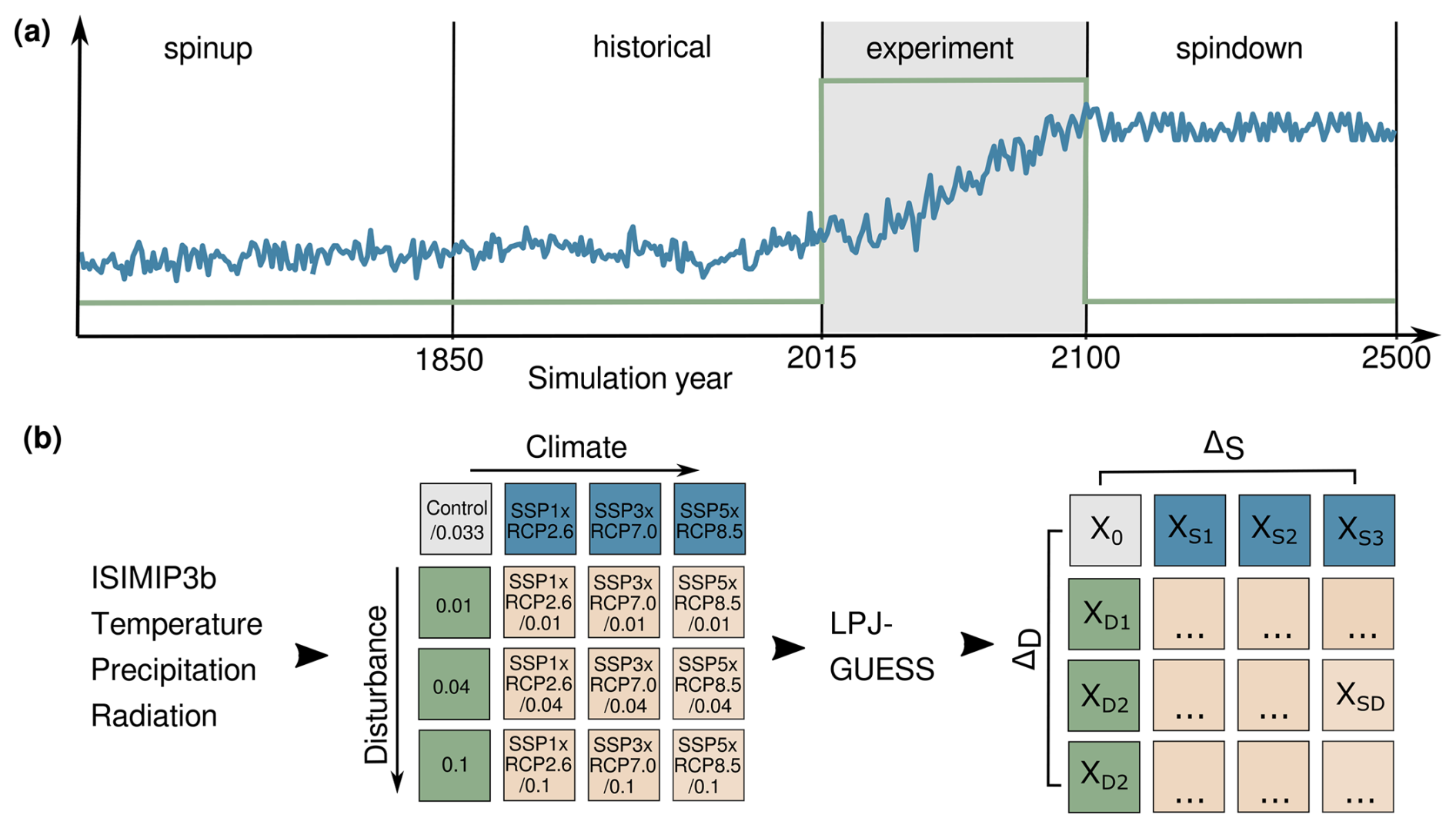
Figure 1 Simulation setup. (a) The elements of a simulation run: spin-up, historic, experimental, and spin-down phase. The blue line indicates an example climate scenario represented by the mean annual temperature, whereas the green line indicates a disturbance regime. Both trajectories are illustrative and not true to scale (see Fig.A1 for the time series of climate variables). (b) Overview of the factorial experiments performed and the methodology for driver attribution.

Table 1 Experimental setup. In the following, we refer to different climates as scenarios, disturbances as regime or probability, and a climate–disturbance combination as a (model) configuration; see also Fig. 1. $\stackrel{\mathrm{‾}}{\mathrm{\Delta }\text{T}}$ is relative to the Control scenario.

2.4 Data analysis

2.4.1 Vegetation composition

We analyze the vegetation composition in terms of fractional plant cover (FPC) and aboveground carbon (AGC). FPC_i describes the fraction of soil covered by a specific PFT i. If the value of total vegetation cover FPC_V is smaller than 1, vegetation does not cover the soil completely, and the bare soil fraction is calculated as 1−FPC_V. Here, FPC can be larger than 1 in the case of dense, multilayered vegetation. We chose FPC as our main variable of interest, as it most directly influences the later calculation of the albedo and evapotranspiration land surface properties. Within this study, we use the term FPC when the soil fraction is included (so this can be larger than 1). We use the fraction of vegetation cover ${\mathit{\chi }}_i^{\mathrm{V}}$ to express the percentage of vegetation FPC (excluding bare soil) that consists of a specific PFT:

$$\begin{array}{}\text{(1)}& {\displaystyle }\text{FPC}={\text{FPC}}_{\mathrm{V}}+{\text{FPC}}_{\text{Soil}},\text{(2)}& {\displaystyle }{\text{FPC}}_{\mathrm{V}}=\sum _i^I{\text{FPC}}_i\forall \text{PFTs }i,\text{(3)}& {\displaystyle }{\mathit{\chi }}_i^{\text{V}}={\displaystyle \frac{{\text{FPC}}_i}{{\text{FPC}}_{\mathrm{V}}}},\text{(4)}& {\displaystyle }{\text{FPC}}_{\text{Soil}}=\text{max}(\mathrm{0},\mathrm{1}-{\text{FPC}}_{\mathrm{V}})={\mathit{\chi }}_{\text{Soil}}.\end{array}$$

For clarity of analysis, we combine all shrub and non-woody PFTs into one non-tree vegetation type. Further, we combine the BNE (“Boreal needleleaf evergreen”) and BINE (“Shade-intolerant boreal needleleaf evergreen”) PFTs to represent all boreal needleleaf (NL) evergreen trees. For the driver attribution (see Sect. 2.4.3), we additionally combine the IBS (“Shade-intolerant (pioneering) broadleaf summergreen”) and TeBS (“Temperate broadleaf summergreen”) PFTs into one broadleaf (BL) summergreen category.

To account for interannual variability, the end-of-century state is represented by the mean and standard deviation over the years from 2085 to 2100. For all other analyses, we smooth data with a 30-year window.

We validate our simulated historical aboveground carbon by comparing it to lidar-based estimates of aboveground biomass across the study region, taken from NASA's North American Carbon Program (NACP) campaign (Neigh et al., 2013, 2015; Margolis et al., 2015). The dataset uses measurements of the years 2005 and 2006 to obtain a point estimate per grid cell. We regridded the data to the LPJ-GUESS resolution of 0.5° and converted them from biomass to aboveground carbon using a conversion factor of 0.5 (Pugh et al., 2024; Sandström et al., 2007). We used aboveground carbon for validation, as carbon cycle indicators are the best-suited diagnostic variables to assess the model performance of LPJ-GUESS.

2.4.2 Biophysical land surface properties

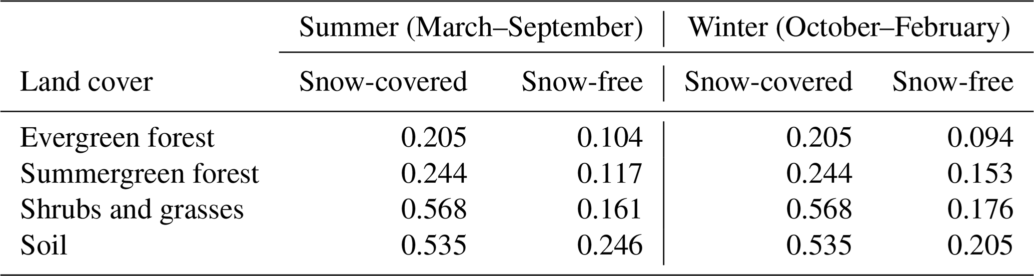
We calculate monthly albedo Λ of a grid cell as the sum of the characteristic seasonal albedo values of different vegetation types Λ_i, multiplied by their respective FPC (adapted from Gregor et al., 2022, and Miller and Smith, 2012):

$$\begin{array}{}\text{(5)}& \begin{array}{rl}\mathrm{\Lambda }& =\sum _i^I\left({\mathit{\chi }}_{\mathrm{S}}{\mathrm{\Lambda }}_{i,\mathrm{S}}+{\mathit{\chi }}_{\mathrm{0}}{\mathrm{\Lambda }}_{i,\mathrm{0}}\right){\text{FPC}}_i\\ & +\left({\mathit{\chi }}_{\mathrm{S}}{\mathrm{\Lambda }}_{\mathrm{Soil},\mathrm{S}}+{\mathit{\chi }}_{\mathrm{0}}{\mathrm{\Lambda }}_{\mathrm{Soil},\mathrm{0}}\right){\mathit{\chi }}_{\mathrm{Soil}},\end{array}\end{array}$$

where χ_S indicates the snow-covered fraction, χ₀ indicates the snow-free fraction, I is the number of PFTs, and χ_Soil is the soil fraction (see Eq. 4).

Characteristic albedo values are taken from Boisier et al. (2013) (see also Table 2). We classify BNS trees as broadleaf summergreen, as previous studies have shown that they are closest in specific albedo (e.g., Hollinger et al., 2010).

LPJ-GUESS outputs the average snow depth h_S (in cm). We calculate the snow cover fraction χ_S from this as follows:

$$\begin{array}{}\text{(6)}& {\mathit{\chi }}_{\mathrm{S}}={\displaystyle \frac{h_{\mathrm{S}}}{\mathrm{0.1}+h_{\mathrm{S}}}},\end{array}$$

following Wang and Zeng (2010).

The model outputs monthly transpiration, soil evaporation, and leaf interception. Total evapotranspiration is calculated as the sum of the three.

Both albedo and evapotranspiration show high interannual variability. Therefore, we performed a two-sided Wilcoxon signed-rank test on a per-grid-cell basis to assess if albedo and evapotranspiration significantly differed from the Control/0.003 (baseline) configuration over the years from 2070 to 2100 (p<0.01).

Table 2 Characteristic albedo values Λ_i for different land cover types adapted from Boisier et al. (2013).

2.4.3 Attribution of drivers

To attribute impacts to drivers in combined climate–disturbance configurations, we assume the observed total effect Δ_SD to be the combination of a climate effect Δ_S, a disturbance effect Δ_D, and an effect Δ_X representing interactions and other nonlinearities (following Verbruggen et al., 2024):

$$\begin{array}{}\text{(7)}& {\mathrm{\Delta }}_{\mathrm{SD}}={\mathrm{\Delta }}_{\mathrm{S}}+{\mathrm{\Delta }}_{\mathrm{D}}+{\mathrm{\Delta }}_X.\end{array}$$

We define an effect Δ_i as follows:

$$\begin{array}{}\text{(8)}& {\mathrm{\Delta }}_i=x_i-x_{\mathrm{0}},\end{array}$$

where x₀ is the Control model state, and x_i is the model state of a configuration i. From our factorial experiments, we can calculate Δ_S, Δ_D, and Δ_SD directly (see Fig. 1b); from there, Δ_X can be calculated as follows:

$$\begin{array}{}\text{(9)}& {\mathrm{\Delta }}_X=x_{\mathrm{0}}+x_{\mathrm{SD}}-x_{\mathrm{S}}-x_{\mathrm{D}}.\end{array}$$

2.4.4 Tools

LPJ-GUESS simulations were performed on the CoolMuc2 Linux cluster of the Leibniz Supercomputing Centre, Munich. All data analyses were executed in the R programming language (R Core Team, 2022) in RStudio version 2022.12.0 using the tidyverse 1.3.2. (Wickham et al., 2019), furrr 0.3.1 (Vaughan and Dancho, 2022), sf 1.0.9 (Pebesma and Bivand, 2023; Pebesma, 2018), terra 1.7.3 (Hijmans, 2023), and rnaturalearth 0.3.2. (Massicotte and South, 2023) packages. Plots were created with ggplot2 (Wickham, 2016) and cowplot 1.1.1 (Wilke, 2020) using the Crameri color scales (Crameri et al., 2020), as implemented by Pedersen and Crameri (2022).

3 Results

3.1 Vegetation composition

Following the spin-up phase, the study region's vegetation is predominantly comprised of needleleaf evergreen trees, accounting for 80 % of the AGC and 59 % of vegetation cover excluding the bare soil fraction (FPC_V; Eq. 3; see also Table B1). Broadleaf summergreen trees (10 % of AGC and 5 % of vegetation cover) and non-tree vegetation (6 % of AGC and 34 % of vegetation cover) are relevant subdominant populations in our simulations. The range of total AGC compares well to satellite-derived data (Fig. B2); however, observed values are lower and feature a pronounced peak around 3 kg m⁻², while the distribution of modeled data is broader. LPJ-GUESS tends to overestimate aboveground carbon in Western Canada, Scandinavia, and western Russia, whereas it underestimates it in Siberia (Fig. B3).

When keeping the disturbances constant at their baseline values, warming reduces the bare soil fraction from 42 % in the Control scenario to 27 % in the strongest warming scenario (SSP5-RCP8.5) by 2100 (first bar of each block in Fig. 2a). Consequently, the fraction of vegetation cover increases. Vegetation composition changes moderately across climate scenarios The relative contribution of non-tree vegetation to vegetation cover decreases, while that of both needleleaf and broadleaf summergreen trees increases. In the strongest warming scenario (SSP5-RCP8.5), vegetation by the end of the century is composed of 69 % needleleaf trees, 21 % broadleaf trees, and 9 % non-tree vegetation (compared to respective values of 57 %, 8 %, and 34 % in the Control simulations). However, in terms of dominant vegetation cover, we see little change across climate scenarios. The majority of grid cells remain dominated by needleleaf evergreen trees, while small areas of the southern ecotone transition to the dominance of either pioneering or temperate broadleaf summergreen species (left panel in Fig. 2c and first row of Fig. B4).

Overall AGC increases with warming from 3.6 to 7.5 kg m⁻² (first bar of each block in Fig. 2b). Broadleaf summergreen trees show above-average gains (from 19 % to 32 % in the strongest warming scenario – SSP5-RCP8.5) at the expense of non-tree and needleleaf evergreen vegetation, with the AGC shares of the latter two categories decreasing from 4 % to 1 % and from 75 % to 67 %, respectively.

In contrast, keeping the climate constant but increasing the disturbance probability barely affects the bare soil fraction χ_Soil but strongly impacts vegetation composition (first block of Fig. 2a). Disturbances strongly reduce the share of needleleaf evergreen trees until they arrive at 5 % of vegetation cover FPC_V (and 3 % of total FPC when including soil; Eq. 1) for the highest disturbance probability of p_D=0.1 in the year 2100. Non-tree vegetation makes up 91 % of all vegetation cover by the end of the century in this configuration, while broadleaf summergreen trees comprise 4 %. Consequently, the vast majority of grid cells are dominated by non-tree vegetation by the end of the century in this disturbance regime for all climate scenarios (center panel of Fig. 2c and right column of Fig. B4).

AGC is strongly reduced by disturbances from 3.6 to 0.5 kg m⁻² for the highest disturbance probability (first block of Fig. 2b). This happens mainly at the expense of trees, while non-tree vegetation gains carbon in both relative and absolute terms.

We see different dynamics in the case of the combined climate–disturbance configurations. In a warmer climate, an increase in disturbance leads to a further reduction in bare soil, for example, reaching 24 % in the high-warming–high-disturbance configuration (SSP5-RCP8.4/0.04), compared to 27 % for high warming alone (Fig. 2a). For the highest disturbance probability of 0.1, the soil fraction increases again to 30 %. In terms of vegetation composition (see also Fig. B4), the disturbance-induced replacement of needleleaf evergreen trees with non-tree vegetation remains the dominant pattern. However, we see an opposing warming-induced increase in broadleaf summergreen trees, which is further exacerbated by disturbance. This increase is nonlinear, reaching its peak for the second-highest disturbance regime p_D=0.04, where broadleaf summergreen trees make up 32 % of vegetation cover FPC_V and 24 % of total FPC (compared to respective values of 21 % and 15 % for warming alone). For the highest disturbance scenario of 0.1, the share of broadleaf summergreen trees is again comparable to the baseline disturbance. We see a similar effect in terms of AGC, where broadleaf summergreen species, for example, make up 54 % of AGC in the combined SSP5-RCP8.5/0.04 configuration by 2100, compared to 32 % for warming alone.

The higher absolute and relative share of pioneering broadleaf vegetation translates to a shift towards broadleaf summergreen dominance in distinct, mostly southern, regions of the study domain (right panel in Fig. 2c). The number of such shifts increases with disturbance and climate (Fig. B4). The majority of remaining grid cells show needleleaf evergreen dominance for a p_D of 0.01 and transition to predominantly non-tree vegetation for a p_D of 0.04.

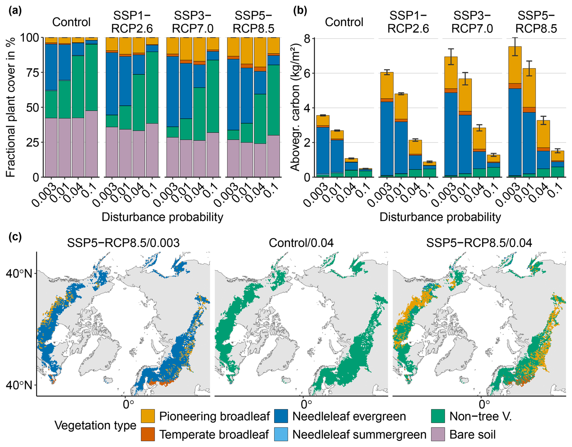
Figure 2 End-of-century vegetation composition across the study domain. (a) Mean FPC by PFT for all scenarios across the study domain. Mean vegetation FPC is always smaller than 1, and the bare soil fraction is calculated as 1−FPC_V. Therefore, absolute FPC equals relative FPC. (b) Aboveground carbon (AGC) per PFT and model configuration. Bars indicate the mean over the years from 2700 to 2100; error bars denote the standard deviation. (c) Spatial patterns of end-of-century dominant vegetation (defined as the largest share of FPC per grid cell) exemplary for a high warming–baseline disturbance (left), Control climate–high disturbance (middle), and high warming–high disturbance configuration (right).

To further disentangle the role of the different drivers in the combined configuration, we next perform the factorial attribution and investigate the relative contribution of drivers over time (Fig. 3). Here, we focus on the SSP5-RCP8.5/0.04 configuration, which showed the strongest interaction effect between climate and disturbance. The SSP1-RCP2.6/0.1 and SSP5-RCP8.5/0.1 configurations are given in the Appendix (Figs. B5 and B6, respectively).

In the climate-only configuration for the SSP5-RCP8.5/0.04 scenario, FPC_V increases until the end of the experimental period (blue lines in Fig. 3a). At the end of the experimental period, FPC_V declines again and stabilizes after 200 years at a Δ_S of 0.1. Needleleaf tree cover χ_NL equally increases, reaches a peak Δ_S of 0.2 mid-experimental phase, and then declines again (Fig. 3b). χ_BL again reaches preindustrial levels 100 years into the spin-down period, and Δ_S is −0.1 at the end of the simulation. By contrast, broadleaf tree cover χ_BL shows a steady increase, by 0.13 at the end of the experimental phase and by 0.37 by the end of the spin-down phase (Fig. 3d). χ_non-tree decreases from the start of the experimental period (Fig. 3f). By the middle of the experimental phase, it has declined by −0.15, and it stays around this value for the rest of the simulation. The response for SSP-RCP2.6 is weaker overall, but it shows similar patterns (Fig. B5)

Disturbances do not have an effect on FPC_V, as visible from Fig. 2a. χ_BL is strongly reduced by disturbance (by −0.24 in this configuration at the end of the experimental period). After disturbance pressure is lifted, it takes 200 years for χ_BL to recover. χ_BL is not affected by disturbances, except for a small increase in the century after disturbance pressure is lifted. χ_non-tree strongly increases, by 0.26 by the end of the experimental phase. Once disturbance pressure is lifted, this reverts (first quickly and then slowly), reaching pre-experimental levels after 250 years. Dynamics for the higher disturbance probability p_D of 0.1 look similar, but total vegetation cover is reduced during the experimental phase, driven by a stronger decimation of evergreen tree cover (Figs. B5 and B6).

In the combined SSP5-RCP8.5/0.04 configuration, increases in FPC_V exceed those of the pure climate forcing. As disturbances do not have an impact for a p_D of 0.04, there is a small interaction effect of 0.03 by the end of the experimental phase and by 0.07 at peak levels 70 years after the experimental phase ends. However, the decrease in χ_BL is stronger than what would have been expected from the net of climate-driven increase and disturbance-driven decreases, leaving an interaction of 0.09 by the end of the experimental phase. In contrast, the combined increase in χ_BL is 2 times the climate-driven effect by the end of the experimental phase and more than 3 times Δ_S at peak levels 30 years later, creating an interaction effect of 0.15 and 0.26, respectively. Here, a notable difference emerges in the case of the SSP1-RCP2.6 scenario, where the interaction effect is much smaller. The picture is less clear in the case of χ_non-tree. Δ_SD follows Δ_D very closely for the first decades of the experimental period before leveling off and declining sharply after the end of the disturbance period. Therefore, the disturbance effect is positive during the experimental period, null at its end, and negative (maximum Δ_x of −0.13) during the spin-down phase. The differences between scenarios are again small in this case.

By the end of the simulation (year 2500), all disturbance-related effects have disappeared (Δ_SD=Δ_S, Δ_D=0, Δ_X=0), and vegetation is in equilibrium again (Δ_SD=const) in all cases, with little difference between scenarios.

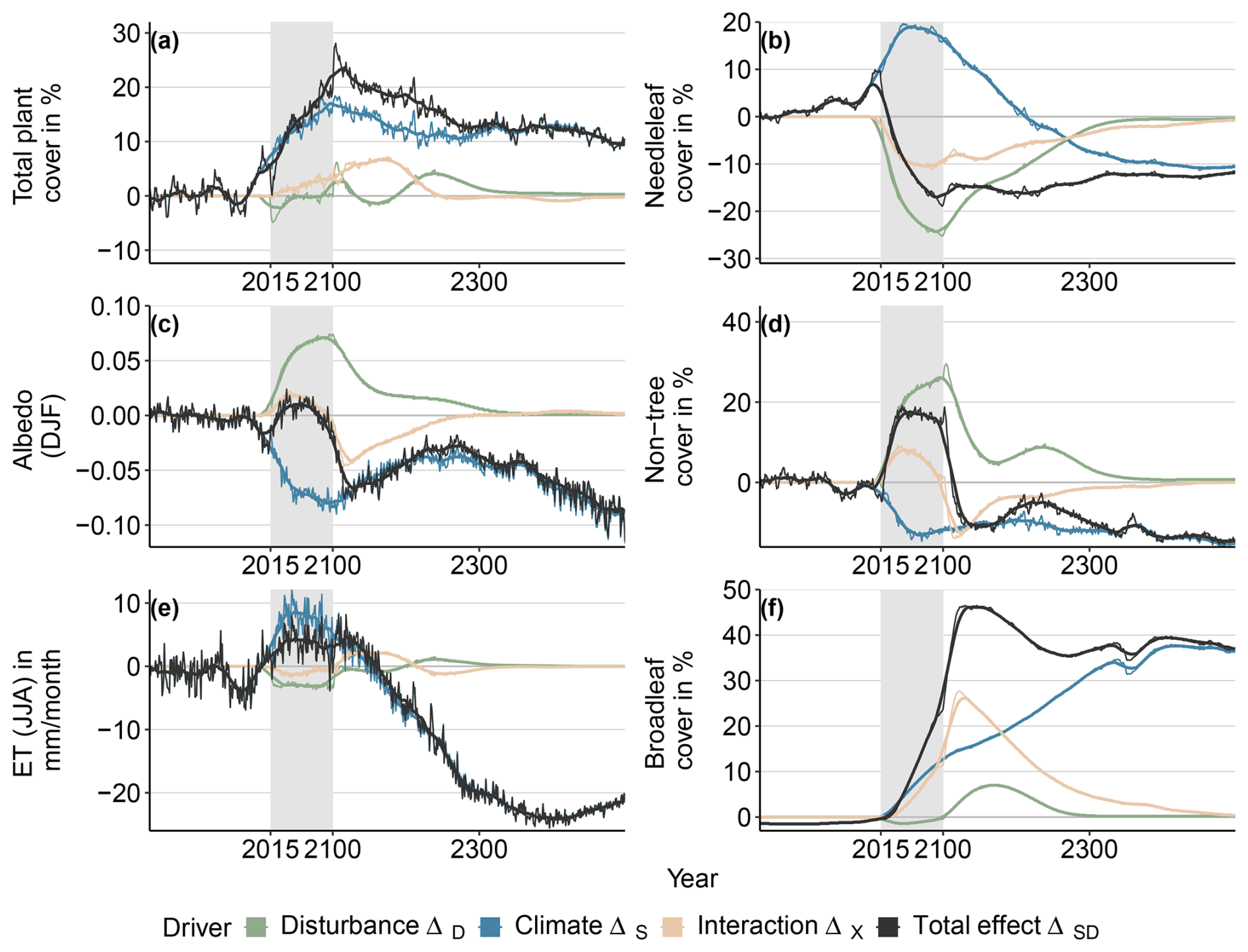
Figure 3 Total effects relative to Control conditions and their attribution to different factors for vegetation composition, albedo, and evapotranspiration for the SSP5-RCP8.5/0.04 model configuration. Gray boxes indicate the experimental period during which the disturbance regime is changed.

Kim et al. (2024)Potter et al. (2020)Rogers et al. (2013)Kuusinen et al. (2006)Wang et al. (2021)Ju et al. (2010)

Table 3 Comparison of simulated monthly values for albedo and evapotranspiration under the Control/historical climate to observed values.

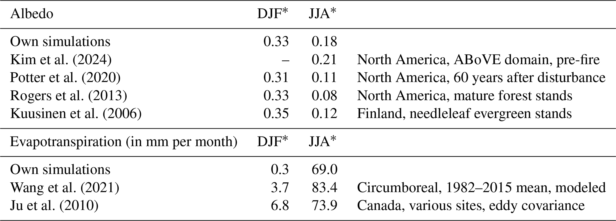
^* The following abbreviations are used in the table: DJF – December–January–February; JJA – June–July–August.

3.2 Surface properties

3.2.1 Albedo

Albedo exhibits pronounced seasonality. Under Control conditions, it reaches peak values of 0.36 ± 0.005 in March and minimum values of 0.18 ± 0.01 in October (Fig. 4a). Simulated winter albedo agrees well with recent observations, whereas summer albedo in our study is at the high end of observations (see Table 3). Warming alone decreases albedo, especially in winter, where maximum values at the end of the century are reduced to 0.33 ± 0.003 in the low-warming scenario (SSP1-RCP2.6) and by 0.25 ± 0.005 in the strongest warming scenarios (SSP5-RCP8.5; solid light- and dark-blue lines in Fig. 4a). The seasonal amplitude in albedo decreases with warming, from 0.18 ± 0.006 for the Control climate to 0.16 ± 0.002 for a low-end warming scenario (SSP1-RCP2.6) and 0.14 ± 0.001 for a high-end warming scenario (SSP5-RCP8.5). Albedo reductions are visible throughout the study region. There are, however, spatial variations with respect to the magnitude, with distinct patches of strong anomalies in Eastern Canada and Eurasia, while other areas, especially regions in Western Canada, Alaska, and southern Russia, show very little change (left panel in Fig. 4c).

An increase in disturbance probability alone has the opposite effect. Increasing p_D from 0.003 to 0.04 while keeping climate constant increases winter albedo to 0.40 ± 0.005 in winter and to 0.21 in summer (dashed pink line in Fig. 4a and pink bars in Fig. 4b). The seasonal amplitude increases to 0.23. The magnitude of change is more uniform throughout the study region (center panel in Fig. 4c).

In the combined scenarios, the pattern of increasing albedo with disturbance probability and decreasing albedo with warming is preserved. However, the net effect differs between scenarios. For the moderate increase in disturbance probability p_D=0.01, the climate effect prevails, resulting in a net decrease in albedo (second group in Fig. 4b). For the highest disturbance probability p_D=0.1, the disturbance effect is stronger, leading to a net increase in albedo compared to baseline disturbance (right group in Fig. 4b). In the middle case of p_D=0.04, we observe a net increase for the SSP1-RCP2.6 scenario and a slight net decrease for the SSP5-RCP8.5 scenario. In the winter months, SSP5-RCP8.5/0.04 is almost on par with the Control/baseline configuration (dashed dark-blue line in Fig. 4a). This change is not uniform across the domain (right panel in Fig. 4c). The SSP5-RCP8.5/0.04 climate–disturbance configuration, for example, shows an albedo increase in distinct regions, whereas it displays albedo decreases in others, resulting in the small net change visible in Fig. 4a and b. While the pure climate–disturbance effect results in significant changes in the majority of the study region, the combined effect can not be separated from interannual variability in this particular configuration.

Investigating the different albedo drivers over time, again for the SSP5-RCP8.4/0.04 example configuration, shows that the climate and disturbance effects constantly increase over the scenario and maintain comparable orders of magnitude, although in different directions (Fig. 3c). At the end of the experimental period, the climate effect is −0.079, while the disturbance effect is 0.068. The interaction effect is small at this point (−0.01). The total albedo effect is, therefore, negligible for most of the scenario (< 0.01), only declining in the last decade of the experimental period to reach −0.023 in 2100. These trends are reversed after the end of the scenario: Δ_SD converges with Δ_S, while Δ_D declines but only approaches 0 after the year 2300. Consequently, we see a counteracting interaction effect until this point as well. The final net albedo effect in simulation year 2500 is −0.088. In both configurations of the high disturbance probability 0.1, the net albedo increased by up to 0.07, due to stronger disturbance-mediated increases as well as interaction effects (Figs. B5 and B6).

3.2.2 Evapotranspiration

Like albedo, evapotranspiration shows high seasonality (Fig. 5a). For all configurations, evapotranspiration is low (< 1 mm per month) in winter (December–January–February – DJF) and reaches the highest levels in July. Peak evapotranspiration reaches 69 ± 2 mm per month in the Control/baseline scenario. Additionally, evapotranspiration shows the strongest interannual variation. Our simulated values are slightly lower than observations but capture the seasonal amplitude well (see Table 3).

Warming alone increases evapotranspiration. The strongest effect is seen in spring, where evapotranspiration (ET) increases by about 4.9 ± 2.3 mm per month for the low-end warming scenario (SSP1-RCP2.6) and 10.2 ± 3 mm per month in the highest warming scenarios (SSP5-RCP8.5; solid light- and dark-blue lines in Fig. 5a and left group in Fig. 5). Notably, maximum evapotranspiration does not differ between the low-end and the high-end warming scenario (76.4 ± 2 and 76.5 ± 3 mm per month, respectively). Climate-induced change in evapotranspiration is seen across the study domain, but the magnitude varies (left panel of Fig. 5c). The strongest decrease is seen in Eastern Canada and southeastern Russia.

Disturbance alone decreases evapotranspiration (dashed pink line in Fig. 5a and pink bars in Fig. 5), for the most intense disturbance regime by −3.47 ± 0.25 mm per month. This decrease is concentrated in distinct areas, while most of the study regions shows no significant change (middle panel of Fig. 5c).

For the majority of combined climate–disturbance configurations, the net effect is an increase in evapotranspiration (Fig. 5b). The exception is SSP1-RCP2.6/0.1 (low-end warming scenario), where evapotranspiration remains unchanged from the baseline, as the climate and disturbance effects offset each other. The spatial analysis shows that, again, evapotranspiration increases in most areas (right panel of Fig. 5 for SSP5-RCP8.5/0.04). However, there are distinct areas that show no significant change. Maximum evapotranspiration is 72.3 ± 2.8 mm per month and 72.7 ± 2.6 mm per month for the SSP1-RCP2.6 and SSP5-RCP8.5 scenarios, respectively, for a p_D of 0.04 (dashed blue lines in Fig. 5a).

Drivers of evapotranspiration effects over time show similar patterns to albedo, although in reversed directions (Fig. 3e). Again, for the SSP5-RCP8.5/0.04 example configuration, climate increases evapotranspiration with peak levels of +8.5 mm per month around the year 2050, while disturbances reduce evapotranspiration. Contrary to albedo, Δ_D is smaller in magnitude than Δ_S, and the net effect over the experimental period is therefore positive, reaching 3.1 mm per month at the end of the scenario. There is no interaction effect. The disturbance effect declines immediately after the end of the scenario. Δ_S and Δ_SD reverse and become negative around 50 years after the experimental period. The final effect at the end of the simulation period is −24 mm per month. Similarly to albedo, the disturbance-induced effect is stronger for a p_D of 0.1, but convergence happens equally fast.

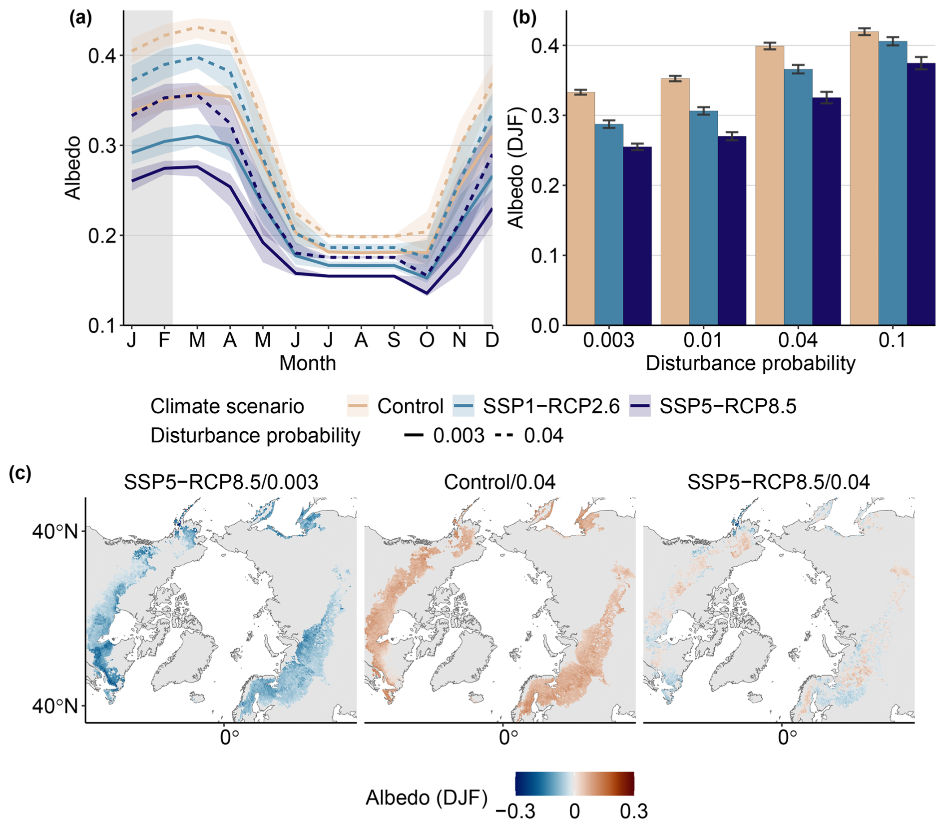
Figure 4 End-of-century albedo across the study domain. (a) Seasonal albedo for selected configurations. Pink lines indicate the Control climate, whereas blue lines show low-end (light blue) and high-end (dark blue) warming. Solid lines indicate baseline disturbance regimes, whereas dashed lines denote a p_D of 0.04. Thick lines show the mean over 2070–2100, whereas ribbons range over individual years. (b) Winter (DJF) albedo for a range of configurations. Bars indicate the mean over the years from 2070 to 2100, while error bars denote ± 1 standard deviation. (c) Spatial patterns of albedo anomaly (relative to Control/baseline) for a high warming–baseline disturbance (left), Control climate–high disturbance (middle), and high warming–high disturbance configuration (right). Stippling indicates areas where albedo does not significantly differ from the Control/0.003 (baseline) configuration (p<0.01).

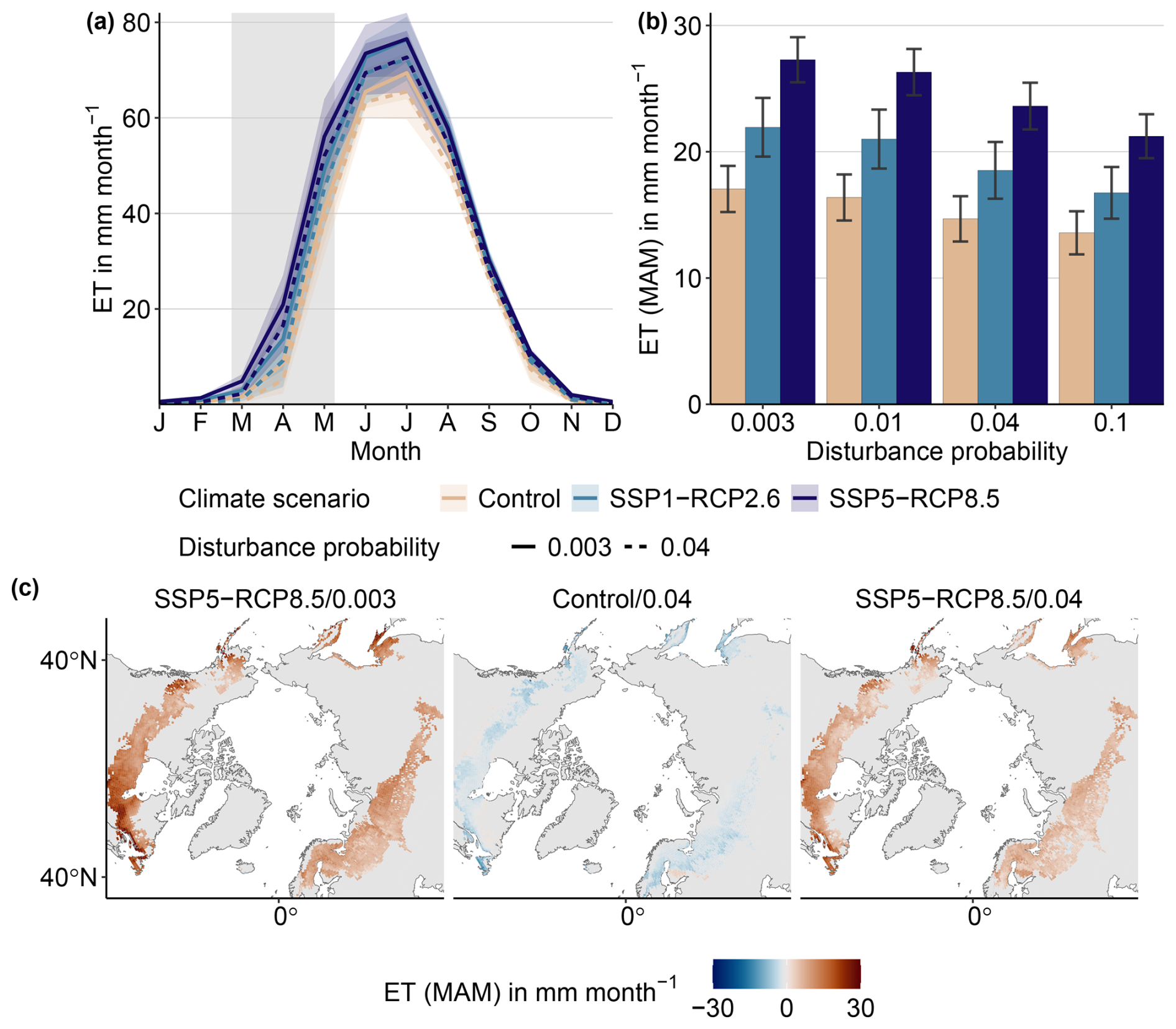
Figure 5 End-of-century evapotranspiration (ET) across the study domain. (a) Seasonal ET for selected configurations. Pink lines indicate the Control climate, whereas blue lines show low-end (light blue) and high-end (dark blue) warming. Solid lines indicate baseline disturbance regimes, whereas dashed lines denote a p_D of 0.04. Thick lines show the mean over 2070–2100, whereas ribbons range over individual years. (b) Spring (March–April–May – MAM) ET for a range of configurations. Bars indicate mean over the years from 2070 to 2100, while error bars denote ± 1 standard deviation. (c) Spatial patterns of ET anomaly (relative to Control/baseline) for a high warming–baseline disturbance (left), Control climate–high disturbance (middle), and high warming–high disturbance configuration (right). Stippling indicates areas where evapotranspiration does not significantly differ from the Control/0.003 (baseline) configuration (p<0.01).

4 Discussion

4.1 Vegetation composition

Historical species distributions produced by our model are in line with observational data and previous modeling studies performed with LPJ-GUESS (see e.g., discussion of Zhang et al., 2013, or Wolf et al., 2008), and the range of total AGC corresponds to observations (Fig. B2). The higher AGC in our simulations is expected, as we simulate potential natural vegetation and do not consider land use change or harvest impacts, which are especially important in Scandinavia and Canada (Pugh et al., 2019b; Potapov et al., 2017; Curtis et al., 2018). Additionally, a disturbance probability of 300 years employed during spin-up is low compared to the observed frequency in some areas. For example, in Western Canada and Alaska, fire return intervals of 100 years are reported, explaining the fact that our model setup leads to an accumulation of aboveground carbon in these regions, compared to observations. The chosen setup is, thus, a trade-off between capturing historical conditions and our goal to obtain largely undisturbed vegetation at the start of the scenario to be able to separate disturbance from climate effects during the experimental period. The species composition under historical climate is robust in our model against a change in disturbance probability within historical return intervals that rarely exceed the 100- to 50-year range (Fig. 2; Burrell et al., 2022; Rogers et al., 2013). Therefore, it is, nevertheless, reasonable to assume that our simulations represent a realistic ecological state.

In general, we find that climate is the dominant driver of the increase in total vegetation cover and carbon, while a complex interplay between climate, disturbance, and their interactions mediates changes at the PFT level and, thus, vegetation composition. Climate change induces an increase in needleleaf evergreen tree cover at the expense of non-tree vegetation, as warming favors the expansion and northward migration of trees (Boulanger and Pascual Puigdevall, 2021; Gustafson et al., 2021; Rees et al., 2020; Zhang et al., 2013), whereas disturbances have the opposite effect, decreasing needleleaf evergreen tree cover and increasing that of non-tree vegetation in our simulations. Depending on the combination of climate and disturbance regime employed, we can thus find a net replacement of non-tree vegetation with needleleaf trees, with opposite or diverging trends in different regions. In the case of broadleaf trees, climate change favors their expansion, whereas disturbance does not affect their FPC share. Therefore, in the absence of interaction effects, disturbance does not affect total vegetation cover, as the replacement of needleleaf evergreen trees with non-tree vegetation results in no net change. Climate, in turn, has a net positive effect, as the expansion of both needleleaf evergreen and broadleaf summergreen trees exceeds what is being replaced by non-tree vegetation.

The interaction between climate and disturbance leads to a combined response that, for needleleaf evergreen trees and non-tree vegetation, is closer to the sole disturbance effect, as would be expected. However, for non-tree vegetation, this is reversed after the end of the scenario, and disturbance effects quickly disappear. Both can be explained by the strong expansion of broadleaf summergreen trees in the combined scenarios. Broadleaf trees substitute both needleleaf evergreen tree and non-tree vegetation after disturbance, preventing their respective climate- and disturbance-driven expansion. Given the assumption that future disturbance rates will significantly surpass historical levels, a decline in needleleaf evergreen tree cover is likely. This is also in line with trends observed over the last decades by researchers such as Wang et al. (2020), who reported a decrease in needleleaf evergreen tree cover and an increase in broadleaf summergreen trees and non-tree vegetation over the years from 1984 to 2014.

Spatial patterns of broadleaf summergreen tree dominance in our simulations correspond to observations from recent field surveys in North America that have reported such vegetation shifts predominantly in Alaska and Western Canada, while the Eastern Canadian Shield and Plains show higher rates of recovery and shifts between different needleleaf species (Figs. 2c and B4; Baltzer et al., 2021). Our model additionally projected state shifts in southern Russia in our simulations, although comparable field surveys from this region are still lacking. Pioneering broadleaf vegetation, such as Aspen or Birch species, is an integral part of succession cycles in many ecosystems of the boreal region (Pfadenhauer and Klötzli, 2020). Thus, one might anticipate their expansion at elevated disturbance levels based solely on a higher proportion of vegetation in an early-successional state in the model. However, when the disturbance rate was increased under a controlled climate, it had minimal impact on these species' absolute or relative abundance. Consequently, their rise cannot be solely attributed to this. Instead, a shift in climatic conditions is additionally needed to render broadleaf species more competitive in post-disturbance recovery (Baltzer et al., 2021; Mekonnen et al., 2019; Wårlind et al., 2014).

An effect that might not be expected at first glance is the resilience of total vegetation FPC to disturbance (Fig. 2a), as a reduction in vegetation density due to high disturbance is likely. We explain this finding in our simulations through the replacement of tree cover with non-tree vegetation. Therefore, while aboveground biomass rapidly decreases, FPC increases due to the higher relative leaf area of non-tree vegetation. This also explains the increase in vegetation cover and the reduction in bare soil with increasing disturbance rate. The undisturbed vegetation composition in our simulations is remarkably resilient against climate change, which also corresponds to recent observations (Kim et al., 2024; Sulla-Menashe et al., 2018). The same is not true of AGC, which is strongly diminished by disturbances (Fig. 2b). Again, this affects mainly needleleaf evergreen trees, while broadleaf summergreen trees and non-tree vegetation are resilient to disturbance and increase their AGC share, also in line with recent field observations (Baltzer et al., 2021; Mack et al., 2021). As our analysis focuses on aboveground processes, it does not allow for further conclusions regarding the impact on the boreal carbon balance, where belowground processes play an important role.

Overall, our findings suggest that modeling results of future vegetation distributions are highly sensitive to the choice of disturbance regime. Therefore, without an accurate representation of disturbance regimes, there is the danger of overestimating the stability of future vegetation. Due to the interaction effects between climate and disturbances, this sensitivity becomes increasingly important with warming, while historical simulations are more robust.

4.2 Land surface properties and potential climate feedbacks

Our simulated historical albedo is high compared to observations in summer, while winter albedo, the main focus of our analysis, shows high agreement. Our results indicate that disturbance and climate have significant but opposing effects on albedo. Therefore, depending on the climate–disturbance configuration, we may see a net increase, a net decrease, or little net change (Fig. 4).

Previous modeling studies, such as Krause et al. (2019), Zhang et al. (2018), or Zhang et al. (2013), have predominantly found albedo decreases of up to −0.25, depending on the climate scenario employed and specific region. This corresponds to our finding for a moderate disturbance scenario (second group in Fig. 4b). These studies did not explicitly consider the effects of disturbance, and the assumed disturbance rates are not always reported. However, it is likely that their results predominantly capture climate effects. Our results indicate that albedo decreases may be reduced or even reversed in a high-disturbance world.

Vegetation shifts are the main driver of albedo change, most importantly the relative shifts between non-tree vegetation and needleleaf evergreen tree cover. Contrary to what previous studies have postulated (Baltzer et al., 2021; Wang and Friedl, 2019; Rogers et al., 2013), the strong increase in broadleaf summergreen tree cover, which we found in our simulations (especially between the years 2100 and 2200), does not translate to an albedo increase. This can be explained by the fact the broadleaf summergreen tree expansion also occurs at the expense of non-tree vegetation and bare soil, which have higher specific albedo. Here, it is important to note that the bare soil fraction in our results is quite high, which of course influences our albedo calculations. It should be noted that the calculated albedo values are highly dependent on the specific albedo values used (Table 2). The values that we used were not derived specifically for the boreal forest, and it is possible that they underestimated the difference in albedo between vegetation types. Indeed, some studies report albedos of 0.6–0.8 in early-successional and/ or broadleaf summergreen forest stands (Kim et al., 2024; Zhang et al., 2018; Rogers et al., 2013). Such values would be unattainable with our approach. In other studies, however, albedo values are in line with our findings, e.g., mean albedo values after disturbance not exceeding 0.5 in Potter et al. (2020). All of these studies report albedo values at the site level, representing mixtures of different vegetation types and soils that are not directly translatable to specific albedo values. If specific albedos for the boreal forest were available, they would greatly improve the accuracy of albedo calculations in the future.

Snow cover dynamics drive the seasonal albedo amplitude but play a minor role in albedo changes in the climate scenarios. This might seem surprising at first, as one might intuitively expect reduced snow cover due to warming. In LPJ-GUESS, warming results in earlier snowmelt and later onset of the snow season over the study area, while snow cover during winter is barely affected by warming (Fig. B7a). This is expected from the climate forcing data used (Fig. B1) and is in line with 21st-century projections from Phase 5 and Phase 6 of the Coupled Model Intercomparison Project as well as previous results from dynamic vegetation models (McCrystall et al., 2021; Krause et al., 2019; Krasting et al., 2013). Uncertainties regarding future snow cover in the climate data used will, of course, in turn, influence our albedo calculations. Here, we also want to note that Potter et al. (2020) found snow cover to be an important predictor of post-fire albedo changes when combining the statistical analysis of recent fire events with climate projections.

Evapotranspiration shows inverse patterns compared with albedo, as climate leads to an increase here, whereas disturbance leads to a decrease. Additionally, in contrast to albedo, the magnitude of change is larger for climate-induced increases. Therefore – within the realistic parameter space assessed in this study – there is no configuration that would achieve a net decrease in evapotranspiration. However, the net effect can be significantly reduced compared to the pure climate effect (Fig. 5).

The impact of disturbances on evapotranspiration is not as well studied as that of albedo. Previous modeling studies found overall increases in evapotranspiration throughout our study domain (Krause et al., 2019; Zhang et al., 2013), even though Krause et al. (2019) found diverging signals when comparing several DVMs. Again, from our results, we can expect those changes to be reduced when accounting for a high-disturbance future.

Climate-driven evapotranspiration change can occur due to direct climate effects, such as temperature or precipitation increase; CO₂-mediated changes in water use efficiency; and climate-modulated vegetation change, which is challenging to untangle. As temperature and precipitation both increase over the course of the scenario, it is likely that climate-induced changes are at least partly driven by direct climate effects. However, as climate is held constant after 2100, we can assume any changes taking place after that are modulated by vegetation.

We expected an increase in evapotranspiration after disturbance due to a higher share of broadleaf summergreen trees and, in turn, a higher leaf area index (LAI), something we cannot confirm from our results. From the individual components making up evapotranspiration, it appears to us that the reduction in needleleaf evergreen tree cover reduces interception and increases runoff, especially in spring, and thus leads to less water being available for evapotranspiration (Fig. B8). Other studies investigating evapotranspiration after fire disturbance have also found reductions, both in the field (Liu et al., 2018) and in modeling results (Bond-Lamberty et al., 2009). It should be noted that some processes governing ecophysiological control on ET are lacking in LPJ-GUESS. Yet, in global simulations, LPJ-GUESS has been shown to accurately simulate ET compared to a number of hydrological datasets (Zhou et al., 2024). However, future model development aiming for a better representation of plant hydraulic strategies may be able to further improve model performance (Papastefanou et al., 2020, 2022; Meyer et al., 2024).

An increase in both albedo and evapotranspiration would result in a cooling of the land surface, while a decrease would have an inverse effect. As LPJ-GUESS was not coupled to an atmospheric model, we cannot determine the actual net effect, especially as other processes, such as cloud formation or surface roughness, can additionally play a role (Gregor et al., 2022; Swann et al., 2010). Previous coupled studies with LPJ-GUESS report a net warming effect due to vegetation dynamics with a high degree of intra-annual and spatial variation (Zhang et al., 2018). Our results indicate that accounting for an increase in disturbance and resulting vegetation changes is lightly to weaken that effect.

4.3 Legacy effects and resilience

We find that disturbance-induced effects on vegetation are long-lasting (∼ several hundreds of years) but ultimately transient and reversible on the centennial timescale if disturbance pressure is lifted again. The tree cover fraction takes the longest to recover, where the total effect converges again with the undisturbed trajectory after up to 400 years.

Our results confirm that the end-of-century vegetation state does not represent an equilibrium, as already shown by researchers such as Pugh et al. (2018). Importantly, this is also true for scenarios in which only the disturbance interval changes (green lines in Figs. 3, B5, and B6). Therefore, we would expect these scenarios to also show sustained change post-2100 before settling in a high-disturbance-intensity equilibrium. Exploring these equilibria and dynamics would be a worthwhile avenue for additional research.

It is interesting to note that, the recovery curves look quite similar across disturbance intensities once disturbances are set back to baseline probabilities, and the convergence timescales of trajectories with different disturbance histories differ little across disturbance intensities and climate scenarios. This indicates that disturbance legacies are dominated by the internal successional dynamics of the vegetation more than previous dynamics. Of course, our stylized scenarios are not a likely long-term scenario, as a return to baseline disturbance regimes or constant climate after 2100 is very unlikely. The question of reversibility is, nevertheless, relevant in the context of forest management and climate mitigation.

However, recovery patterns need to be interpreted cautiously, as there are a number of limitations in the implementation of establishment and disturbance in the model: in LPJ-GUESS, there is no interaction between grid cells for reasons of computational efficiency; thus, there is no lateral exchange of seeds, which would control spatial migration. Rather, migration is emulated through a background establishment rate (a small rate of establishment that will always occur as soon as PFTs are within their bioclimatic limits). This may lead to a faster northward expansion of trees than if migration would be limited by seed dispersal (Zani et al., 2023). Additionally, the production of offspring (and thus establishment) can occur once a plant is productive (there is no maturation period). This means that, by model design, regeneration failure – eroding of seed banks through overly frequent disturbances (Turner et al., 2019; Hansen et al., 2018) – cannot occur. Here, different reproductive strategies, e.g., serotony or resprouting, would also be important to consider (Baltzer et al., 2021; Hansen et al., 2021). Therefore, while our results indicate a general possibility for recovery, the conditions under which this is a realistic scenario need to be explored in more detail in the future.

In this context, disturbance type is also important. Here, we employed a standardized disturbance event to reduce dimensionality in our simulations and ensure controlled experiments. However, it is important to keep in mind that specific disturbances can have additional effects that we do not consider here. For example, wildfire affects soil conditions, via processes such as the burning of the peat layer and changes in nutrient cycling (Mack et al., 2021; Mekonnen et al., 2019). Further, our disturbance dynamics are uniform in space and time and not linked to vegetation type, as, for example, a detailed fire disturbance module would be. In that case, we would especially expect disturbance frequency and impact to differ with vegetation type. Broadleaf summergreen trees are less susceptible to fire, and the literature suggests that broadleaf summergreen tree dominance could maintain itself through fire suppression (Hansen et al., 2021; Mekonnen et al., 2019; Johnstone et al., 2016, 2010). Wind damage and pathogen attacks are equally linked to climate conditions and species compositions (Mitchell, 2013; Seidl et al., 2017). Additionally, there are interaction effects of disturbances. For example, deadwood from windthrow provides a habitat for bark beetles or fuel for wildfires (Seidl et al., 2017). Taken together, all of these limitations suggest a potential overestimation of the recovery ability of vegetation in the model.

Disturbance-induced changes in land surface properties are mainly driven by changes in non-tree vegetation cover, which is less subject to legacy effects and internal dynamics than tree cover and more directly controlled by climate. Therefore, both albedo and evapotranspiration recover quickly once disturbance pressure is lifted again, and legacy effects disappear after approximately 25 years. We stress that our results provide information on the potential ability to recover, rather than a realistic projection of likely dynamics after the 21st century. With sustained disturbance regimes, the respective changes in land surface properties would likely persist.

5 Conclusions

In this study, we investigated the relative impact of climate change, intensifying disturbance regimes, and their interaction on boreal vegetation and land surface properties. We found that, in general, climate drives shifts towards denser and more forested vegetation, while disturbances reduce the prevalence of trees in favor of shrubs and grasses. The interaction between climate and disturbances increases broadleaf summergreen tree cover, causing shifts from needleleaf evergreen and non-tree vegetation to broadleaf summergreen dominance. The shifts that we observe are not driven by prescribed bioclimatic limits but are, rather, an emergent feature of the model, arising from a shift in competitive balance. This highlights the ability of LPJ-GUESS to realistically capture the influence of climate change on succession and thus post-disturbance recovery dynamics.

In our simulations, disturbances affect albedo and evapotranspiration. In both cases, the disturbance effect opposed the pure climate effect, while interactions between the two factors played a minor role. ET is more closely coupled to direct climate effects, with vegetation changes playing a subordinate role. In contrast, vegetation shifts (due to both disturbances and warming) are the main drivers of observed albedo changes. Here, disturbance-induced effects have the potential to weaken or even reverse climate-induced changes.

Disturbances caused long-lasting legacies in vegetation composition, which only regenerated on the centennial timescale. In contrast, albedo and evapotranspiration recovered on a decadal timescale. Therefore, while our results show the ability of disturbances to severely disrupt land surface–atmosphere interactions, they also highlight the theoretical potential for regeneration. Better understanding how seed dispersal and maturation would affect this regeneration potential remains an important avenue for future research.

We find simulated future vegetation distributions to be highly sensitive to the choice of disturbance regime. Due to the interaction effects between warming and disturbances, this sensitivity becomes increasingly important when moving into a high-warming future, while historical simulations are more robust against the choice of disturbance regime. Without an accurate representation of disturbance, there is a risk of misjudging future vegetation composition and resulting land surface properties.

Appendix A: Methods

Table A1 Overview of relevant PFT-related parameters: Leaf – leaf type (needleleaf – NL; broadleaf – BL); Pheno – phenology (evergreen – EG; summergreen – SG); Shade – shade tolerance; $t_{t,c/s,min/max}^{\mathrm{E}/\mathrm{S}}$ – coldest (min)/warmest (max) month temperature needed for establishment (E)/survival (S); GDD5${}_{\min ,i}^{\mathrm{E}}$ – growing season temperature sum; L_i – longevity. Readers are referred to Table A2 for the definitions of the PFTs listed in this table.

Table A2 Overview of the PFTs used.

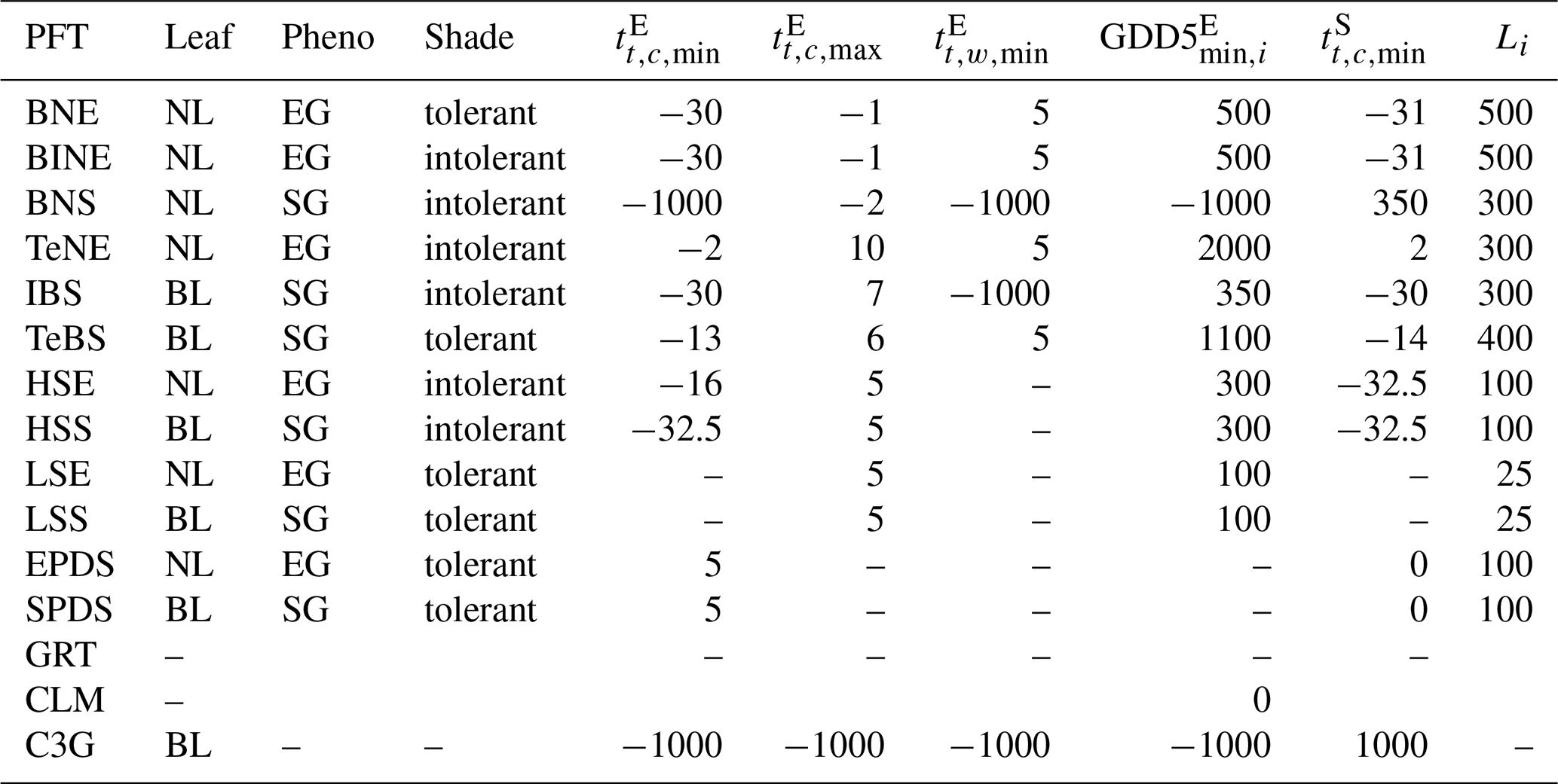
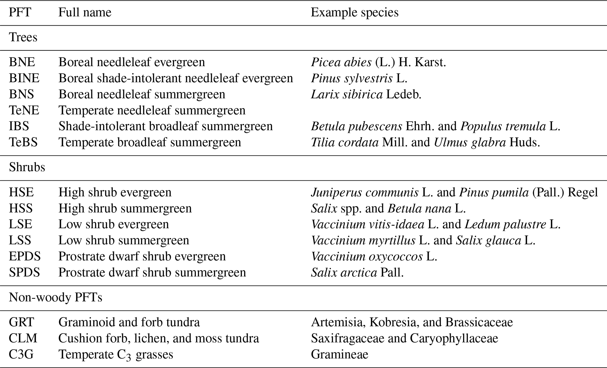
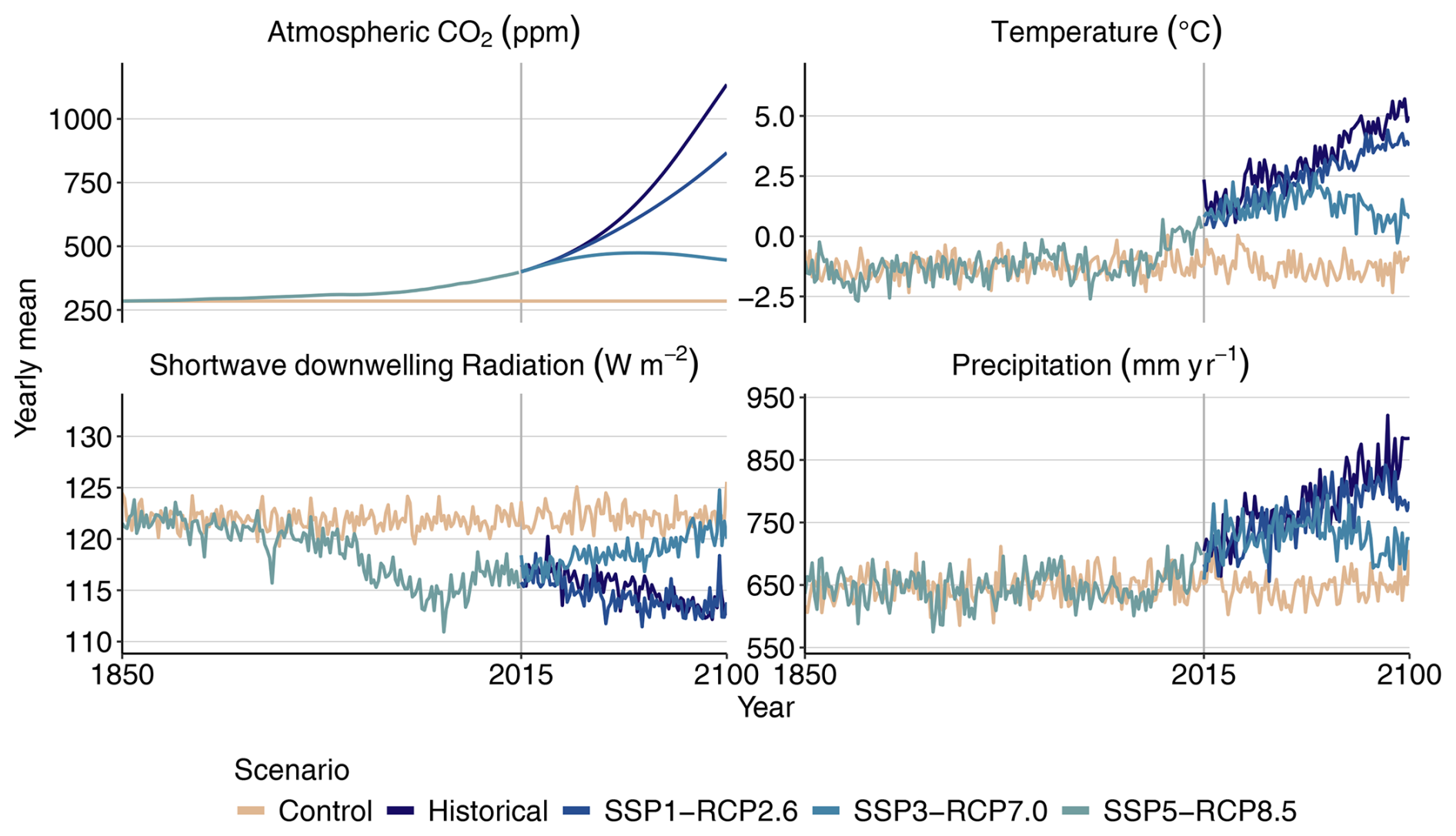
Figure A1 Climate data used to force the simulations. Note that model runs continue until 2500, with further recycling of data of the years 2095–2100.

Appendix B: Results

Table B1 Average vegetation composition at the end of the spin-up period (spatial and annual mean across the years from 1850 to 1880). Factorial simulations are restarted from this state.

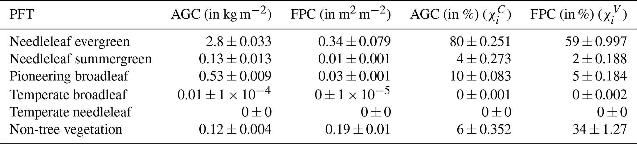
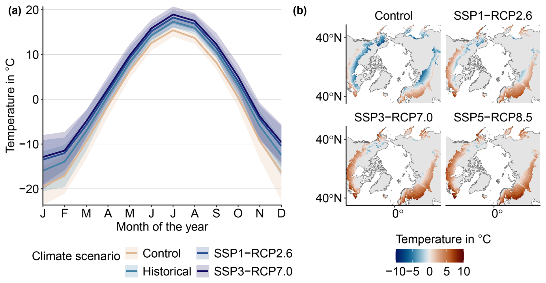
Figure B1 Overview of the MRI-ESM2 temperature data used to force LPJ-GUESS. (a) Seasonal curves, averaged over the years from 2070 to 2100. The ribbon indicates spread over years. For a similar depiction of precipitation, see Fig. B7b. (b) Maps averaged over the same time frame.

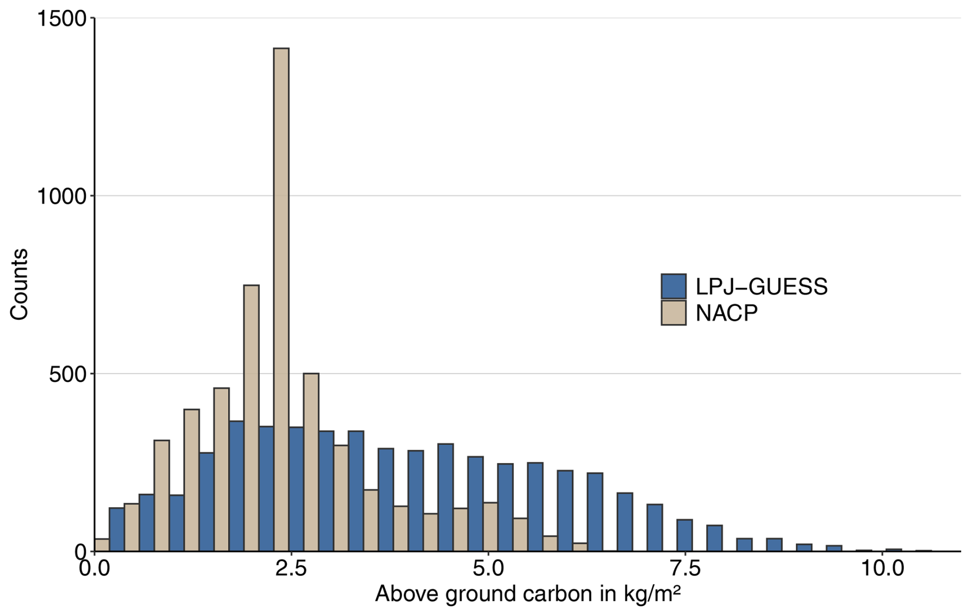
Figure B2 Comparing the aboveground carbon (AGC) simulated by LPJ-GUESS with remotely sensed AGC from NASA's NACP mission. Both datasets show the year 2005.

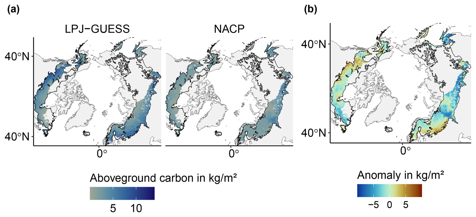
Figure B3 Comparing aboveground carbon (AGC) simulated by LPJ-GUESS with remotely sensed AGC from NASA's NACP mission: (a) absolute values and (b) anomalies. Both datasets show the year 2005 across the spatial domain. The black outline indicates the boreal biome as defined by Olson et al. (2001).

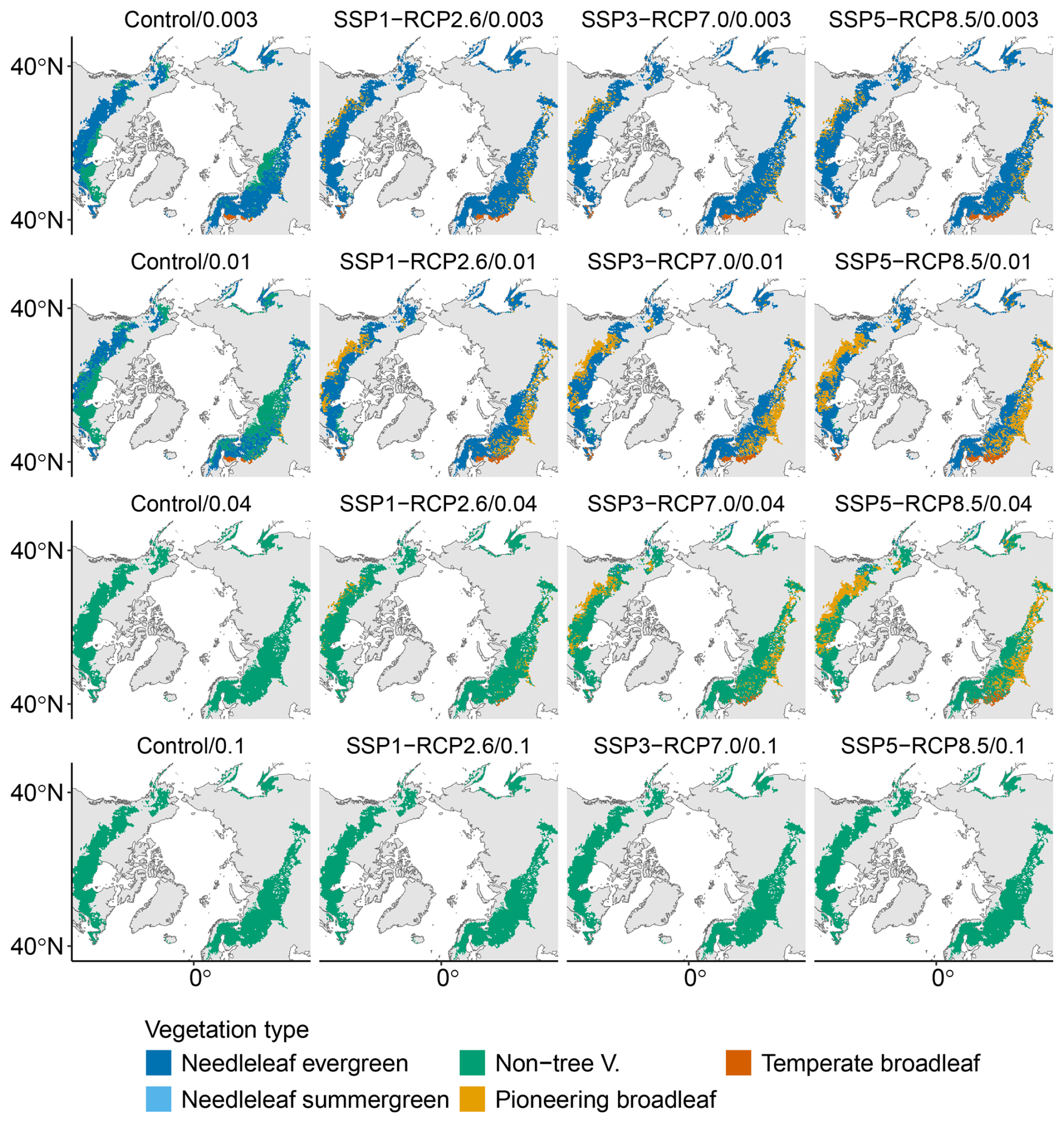
Figure B4 End-of-century dominant vegetation type for all configurations. Rows show a shift in climate, whereas columns show a shift in disturbance regime.

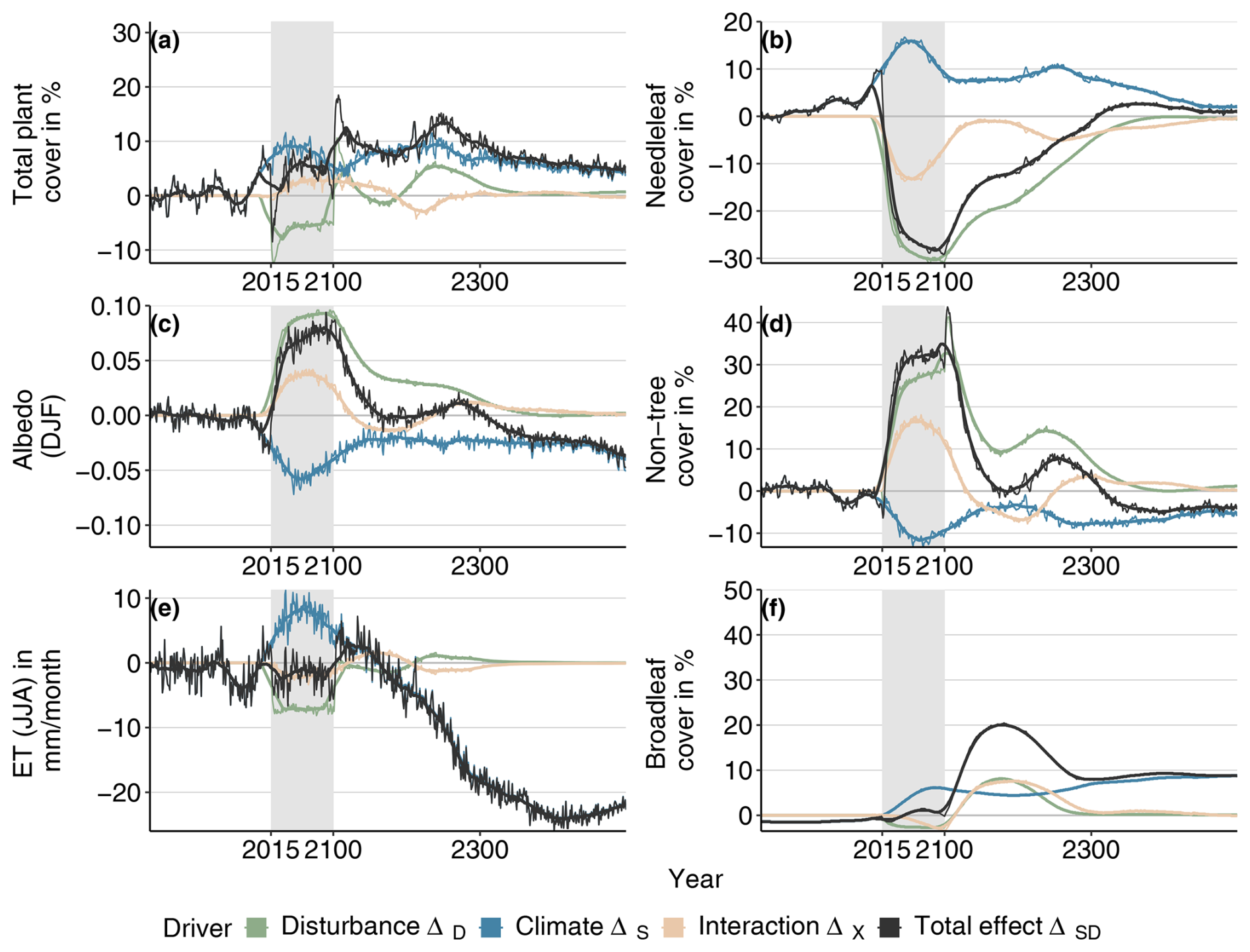
Figure B5 Total effects relative to Control conditions and their attribution to different factors for vegetation composition, albedo, and evapotranspiration for the SSP1-RCP2.6/0.1 model configuration. The black line indicates the difference between the baseline (Control/0.003, baseline) and the SSP1-RCP2.6/0.1 combined scenario, the blue line represents the difference between the baseline and the SSP1-RCP2.6/0.03 scenario, and the green line denotes the difference between the baseline and the Control/0.1 scenario. The pink line represents the interaction effect (difference between the black line and the sum of the green and the blue lines). Gray boxes indicate the experimental period during which the disturbance regime was changed.

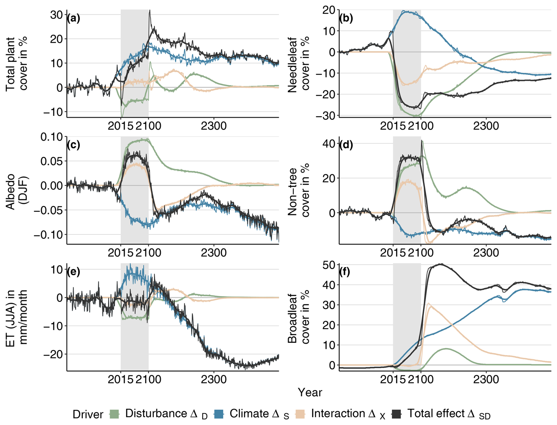
Figure B6 Total effects relative to Control conditions and their attribution to different factors for vegetation composition, albedo, and evapotranspiration for the SSP5-RCP8.5/0.1 model configuration. The black line indicates the difference between the baseline (Control/0.003, baseline) and the SSP5-RCP8.5/0.1 combined scenario, the blue line represents the difference between the baseline and the SSP5-RCP8.5/0.03 scenario, and the green line denotes the difference between the baseline and the Control/0.1 scenario. The pink line represents the interaction effect (difference between the black line and the sum of the green and the blue lines). Gray boxes indicate the experimental period during which the disturbance regime was changed.

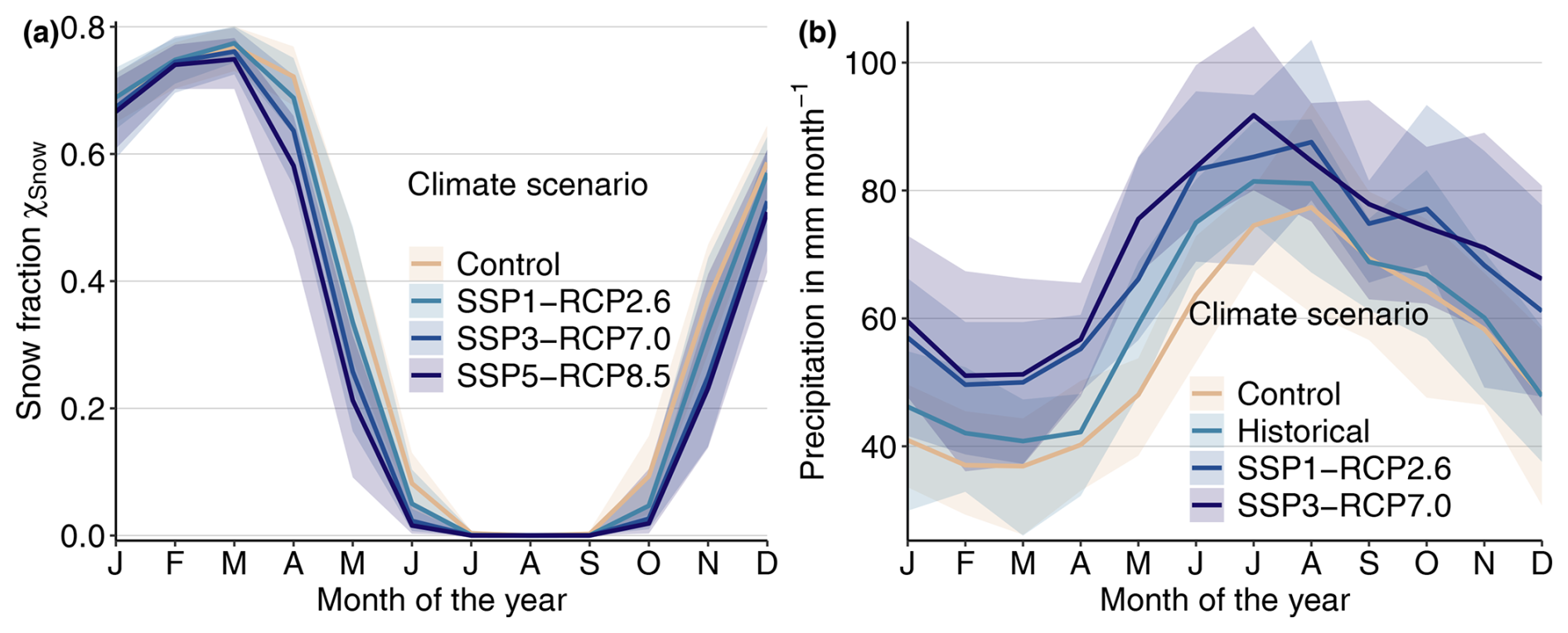
Figure B7 End-of-century seasonal curves of the snow cover fraction (a) and precipitation (b). Thick lines indicate the mean over the years from 2070 to 2100, whereas ribbons indicate the range over individual years.

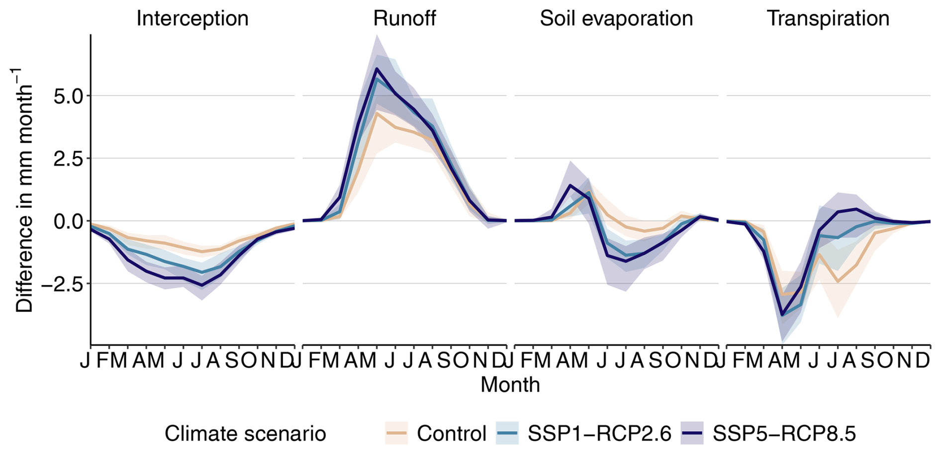
Figure B8 End-of-century seasonal curves of the difference in state Δ_D between a p_D of 0.00$\stackrel{\mathrm{‾}}{\mathrm{3}}$ and 0.04 for different evapotranspiration components as well as surface runoff. Evapotranspiration is the sum of interception, soil evaporation, and transpiration. The ribbon indicates the spread of the years 2070–2100.