Evolution of biogeochemical properties inside poleward undercurrent eddies in the southeast Pacific Ocean

Oceanic eddies are ubiquitous features of the circulation thought to be involved in transporting water mass properties over long distances from their source region. Among these is a particular type that has a core within the thermocline with little surface expression. Despite their significance, their role in ocean circulation remains largely undocumented by observations. This study characterizes the variations in internal biogeochemistry, disparities with external properties, and processes influencing the dissolved oxygen budget of poleward undercurrent eddies (PUDDIES) during their transit to oceanic waters. Employing a high-resolution coupled simulation of the Southeast Pacific, we document biogeochemical properties and processes associated with the nitrogen cycle inside PUDDIES and contrast them with those of the surrounding environment. Our findings reveal that PUDDIES capture a biogeochemical signal contingent upon their formation location along the coast, particularly associated with the core of the Peru–Chile Undercurrent at the core of the oxygen minimum zone (OMZ). While permeability at the periphery facilitates exchange with external waters, thereby modulating the original properties, the core signal retains negative oxygen (O₂) anomalies and positive anomalies of other biogeochemical tracers. These anomalous conditions result in tracer values exceeding the 90th percentile of their distribution in the open ocean, in contrast to the formation zones, where anomalies only surpass the 50th percentile. This indicates that PUDDIES may play a role in modulating the average properties of the open ocean. Suboxic (O₂<20 µM) cores are prevalent near the coast but decrease in abundance with distance from shore, giving way to a predominance of hypoxic (20 µM < O₂<45 µM) cores (predominating at 60 % in the open sea), suggesting core ventilation during transit. The principal mechanism governing O₂ input to or output from the eddy core entails lateral and vertical advection, with vertical mixing supplying O₂ to a lesser extent. Biological activity consumes O₂ inside PUDDIES for around 6 to 12 months, especially intensely for the first 100 d, thus facilitating the persistence of low O₂ conditions and extending the lifetime of biogeochemical anomalies within the core (up to 800 km offshore). Ammonium and nitrite deplete earlier in the eddy core with a decay rate greater than that of nitrate and nitrous oxide, while these accumulate in the open sea (up to 16 % and 100 % higher than the mean state, respectively). Our results suggest that southern regions of the southeast Pacific OMZ undergo greater deoxygenation and nutrient enrichment due to PUDDIES compared to northern regions. However, the combination of various physical conditions can generate zones with more pronounced changes in the nitrite (subsurface water masses due to interactions with the PUDDIES, such as at 30° S). The maximum contribution of NO${}_{\mathrm{2}}^{-}$ takes place in particular along this latitude, with a 460 % increase compared to the mean state, near the coastal zone.

In summary, PUDDIES formed along the Chilean coast capture distinct biogeochemical “signatures” depending on where they form. In the north, minimal ventilation fosters suboxic conditions and denitrification – leading to deficits of nitrate (NO${}_{\mathrm{3}}^{-}$) and nitrous oxide (N₂O) but high NO${}_{\mathrm{2}}^{-}$ and ammonium (NH${}_{\mathrm{4}}^{+}$) – whereas central and southern subregions show increased NO${}_{\mathrm{3}}^{-}$ and higher N₂O. Moreover, cross-shore exchange between Equatorial Subsurface Water and Subantarctic Water further amplifies this variability, giving rise to eddies with diverse nutrient and oxygen properties as they move offshore.

1 Introduction

Oxygen plays a fundamental role for life in the ocean, and numerous processes regulate its concentration in the water column. In subsurface waters (100–800 m depth), oxygen concentrations (O₂) decrease significantly due to the decomposition of organic matter and limited ventilation, leading to the formation of oxygen minimum zones (OMZs) in eastern boundary upwelling systems (EBUS; Wyrtki, 1962; Helly and Levin, 2004; Karstensen et al., 2008; Paulmier and Ruiz-Pino, 2009; Stramma et al., 2010). Under these conditions of low oxygen in the subsurface (i.e., dissolved O₂ less than 20 µM), heterotrophic metabolic processes are important, dominated by the activity of bacteria and archaea, resulting in significant shifts in biogeochemical cycles (Lam et al., 2009; Paulmier and Ruiz-Pino, 2009; Wright et al., 2012).

The nitrogen cycle in the oceans involves various chemical species with different oxidation states. Outside the OMZ, where conditions are oxygenated, dinitrogen (N₂) is transformed into ammonium (NH${}_{\mathrm{4}}^{+}$), nitrite (NO${}_{\mathrm{2}}^{-}$), and nitrate (NO${}_{\mathrm{3}}^{-}$) through nitrification, with nitrous oxide (N₂O) produced as a byproduct. However, within the OMZ, where O₂ is depleted, nitrate becomes the primary oxidant, triggering denitrification. In this process, nitrate is reduced to gaseous forms (N₂ and N₂O), which can then be released into the atmosphere. This process has implications for primary production, carbon sequestration, and the release of N₂O into the atmosphere, a potent greenhouse gas (Goreau et al., 1980; Fauzi et al., 1993; Sarmiento and Gruber, 2006; Lam et al., 2009; Paulmier and Ruiz-Pino, 2009; Wright et al., 2012).

The southeast Pacific Ocean is the site of one of the most extensive and shallow OMZs (Paulmier and Ruiz-Pino, 2009), where even anoxic conditions can be observed (Ulloa et al., 2012). Several authors have determined the vertical and zonal (offshore) extent of the OMZ, which exhibits significant seasonal variability, modulated both meridionally by subsurface currents toward the pole and zonally by mesoscale processes (jets, eddies, fronts, filaments, etc.; Bettencourt et al., 2015; Chaigneau et al., 2011; Grados et al., 2016; Hormazabal et al., 2013; Morales et al., 2012; Stramma et al., 2013; Vergara et al., 2016; Pizarro-Koch et al., 2019). These processes result in changes in water mass properties and together contribute up to a 25 % reduction in O₂ volume during spring (Pizarro-Koch et al., 2019).

Furthermore, future projections suggest the expansion of these O₂-depleted zones through global warming (Matear and Hirst, 2003; Stramma et al., 2010; Oschlies et al., 2018), although uncertainties remain (Almendra et al., 2024). The increase in sea surface temperature will affect O₂ solubility, and enhanced water column stratification will impact a range of biological processes that influence O₂ concentrations (Couespel et al., 2019; Keeling et al., 2010; Matear and Hirst, 2003; Oschlies et al., 2018; Schmidtko et al., 2017). In addition, various mechanisms can potentially modify ventilation processes, leading to changes in subsurface water properties. While in current generation climate models, the changes in mean circulation either in the tropics or the high-latitudes, mediated by diapycnal mixing, are invoked to explain the ventilation process (Pitcher et al., 2021), regional modeling studies highlight the importance of mesoscale dynamics, such as mesoscale eddies and zonal jets, in expanding and ventilating oceanic zones with oxygen deficits (Bettencourt et al., 2015; Auger et al., 2021; Calil, 2023). The regional models also provide a more realistic representation of the OMZs than the climate models that do not resolve sub- to mesoscale dynamics. This is why understanding the role of mesoscale dynamics on the O₂ and carbon cycles in EBUS has been a key focus of research in recent years.

“Poleward undercurrent eddies” (PUDDIES) are types of subsurface or intrathermocline eddies characterized by coherent anticyclonic lenticular-shaped vortices with cores located within the pycnocline and relatively homogenous interior waters (Dugan et al., 1982; McWilliams, 1985; Kostianoy and Belkin, 1989). PUDDIES originate in the EBUS (Frenger et al., 2018) due to the interaction of the poleward-flowing current with the continental slope, generating submesoscale instabilities with anticyclonic vorticity, subsequently forming these characteristic mesoscale structures (Hormazabal et al., 2013; Combes et al., 2015; Molemaker et al., 2015; Thomsen et al., 2016; Contreras et al., 2019). These eddies represent 30 %–55 % of the anticyclone eddies originating in the EBUS (Pegliasco et al., 2015; Combes et al., 2015) with cores that are warmer, saltier, O₂-depleted, and nutrient-enriched relative to surrounding waters (Collins et al., 2013; Hormazabal et al., 2013; Morales et al., 2012; Johnson and McTaggart, 2010). Therefore, PUDDIES can play a crucial role in transporting these water properties hundreds or thousands of kilometers offshore to subtropical gyres, potentially contributing to the expansion of the OMZ beyond the coastal region (Frenger et al., 2018). Observations of low O₂ events in open ocean regions provide support for this idea (Lukas and Santiago-Mandujano, 2001; Johnson and McTaggart, 2010; Cornejo D'Ottone et al., 2016; Schütte et al., 2016; Stramma et al., 2013, 2014; Karstensen et al., 2015), with further evidence of biogeochemical processes typically observed only in the OMZ, such as N₂O production (Cornejo D'Otonne et al., 2016; Arévalo-Martínez et al., 2016; Grundle et al., 2017) and nitrogen loss through denitrification (Altabet et al., 2012; Löscher et al., 2015). Additionally, the observed O₂ utilization rates within the eddy cores range from 0.29 to 44 nmol O₂ L⁻¹ d⁻¹, which is up to 3 to 5 times higher than in the surrounding waters (Cornejo D'Ottone et al., 2016; Karstensen et al., 2015). There is evidence of harboring microbial communities and metabolisms associated with low-oxygen environments that persist even when the eddies enter highly oxygenated waters, a phenomenon known as the “stewpot effect” (Löscher et al., 2015; Frenger et al., 2018).

The Southeast Pacific (SEP) is characterized by extensive subsurface mesoscale eddy activity with radii ranging from ∼25 to ∼50 km and cores of ∼500 m of vertical extent (Chaigneau et al., 2009; Hormazabal et al., 2013; Combes et al., 2015; Frenger et al., 2018). They transport a total volume of approximately 1 Sv (1 Sv = 1×10⁶ m³ s⁻¹) westward with an average velocity of ∼2 km d⁻¹ (Hormazabal et al., 2013). The cores of these eddies exhibit homogenous salinity profiles (>34.5) and low O₂ concentrations (<1.0 mL L⁻¹), linking them to Equatorial Subsurface Water (ESSW) transported poleward by the Peru–Chile Undercurrent (PCUC; Hormazabal, 2004; Colas et al., 2012; Hormazabal et al., 2013). Generally, the low values of O₂ in subsurface eddies are related to higher concentrations of nitrate, phosphate, and silicate (Czeschel et al., 2015). However, under suboxic conditions (O₂<20 µM), the prevailing anaerobic metabolism is denitrification, where nitrate is utilized as an electron acceptor, leading to increased production of NO${}_{\mathrm{2}}^{-}$ and N₂O (Goreau et al., 1980; Fauzi et al., 1993; Lam et al., 2009; Wright et al., 2012). Within these eddies, various biogeochemical processes coexist that are highly sensitive to O₂ variations, while physical processes modulate biogeochemical patterns through vertical and lateral mixing, submesoscale stirring, or mass exchange with water masses from different origins through turbulent advection (José et al., 2017; Karstensen et al., 2017; Lovecchio et al., 2022).

This complex of processes involved during the life cycle of a PUDDY, along with the lack of continuous in situ measurements, limits our understanding of nutrient recycling throughout their lifetime and the balance between processes controlling the rate of change of O₂ and nutrients. In the present study, we aim to characterize the internal biogeochemistry of eddies formed under various low-oxygen conditions in the SEP. We analyze the physical and biogeochemical factors influencing the variability in the lifespan of elements trapped within the PUDDIES, with a particular focus on those related to the nitrogen cycle as they travel across the OMZ toward better-ventilated oceanic waters. Specifically, we document the evolution of water mass properties and processes inside PUDDIES with contrasting initial O₂ concentrations (suboxic versus hypoxic) to evaluate their role in maintaining the OMZ. Additionally, we aim to address knowledge gaps in the biogeochemical dynamics of this type of eddy, stemming from the lack of observational data, particularly in the SEP. To quantify the changes PUDDIES undergo, we use a regional coupled biogeochemical model simulation.

Our approach involves a robust statistical analysis of contrasting water mass properties inside and outside the PUDDIES. First, we characterize the initial biogeochemical signal from their formation to assess how, and to what extent, the biogeochemical properties of PUDDIES' cores vary across different regions of the SEP. Second, we quantify how these properties influence the subsurface waters through which PUDDIES travel, evaluating the balance of processes involved.

The structure of this study is as follows: Section 2 details the model and methods used for the identification and characterization of PUDDIES. Section 3 describes the biogeochemical characterization inside and outside the PUDDIES, changes in the O₂ budget, and variations in biogeochemical properties from the coastal to oceanic zones. Section 4 discusses the results, and Sect. 5 presents the main conclusions and future projections.

2 Methods

2.1 Regional biogeochemical coupled model

We used a high-resolution, coupled physical–biogeochemical model simulation of the SEP that considers the main processes involved in the transformation of water masses relevant to OMZ variability and the dynamics of the Peru–Chile Undercurrent (PCUC). This current plays a significant role in generating PUDDIES and in the southward extension of the OMZ in the Peru–Chile EBUS.

The physical dynamics were simulated using the Regional Ocean Modeling System (ROMS), a regional ocean circulation model that solves the primitive equations with free surface and sigma coordinates (Shchepetkin and McWilliams, 2005). ROMS was coupled with the biogeochemical model BioEBUS, specifically developed for eastern boundary upwelling systems (EBUS) and based on the nitrogen cycle using the N₂P₂Z₂D₂ model formulation (Koné et al., 2005; Gutknecht et al., 2013). We adopted the same configuration as specified in several other studies in the region (Dewitte et al., 2012; Vergara et al., 2016; Pizarro-Koch et al., 2019). The model has a spatial resolution of $\mathrm{1}/\mathrm{12}$°, with 37 vertical levels. We used 3 d mean outputs, which are suitable for resolving mesoscale features. The overall domain covers the latitudinal range of 12° N to 40° S from the coast to 95° W, although the present study focuses on latitudes off the coast of Chile between 20 and 40° S (Fig. 1a). The simulated period was from 2000 to 2008.

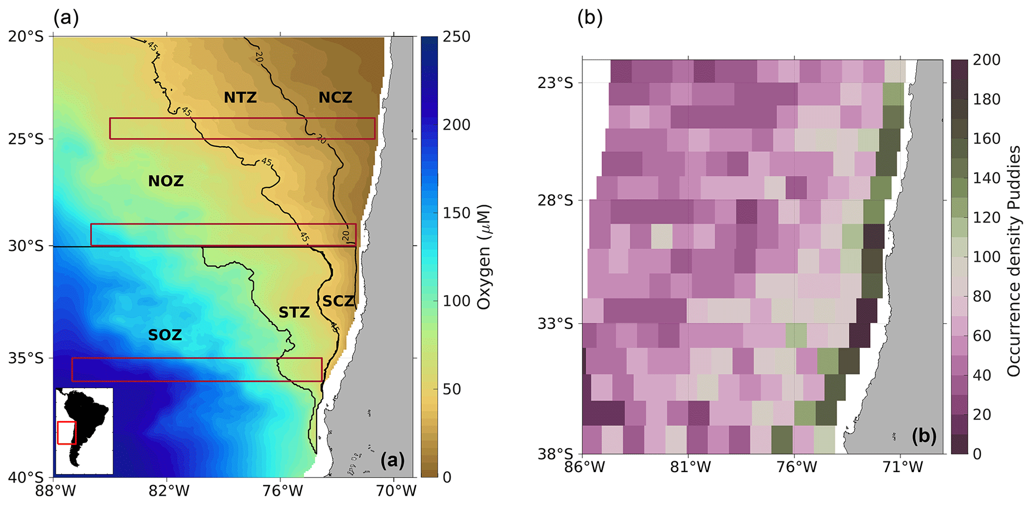
Figure 1 (a) Modeled dissolved O₂ climatology off the Chilean coast and (b) spatial distribution of the occurrence density of PUDDIES identified over the 9-year period. Oxygen was considered to be in the isopycnal layer of 26.6 kg m⁻³, representative of the OMZ core (defined with the S_core layer; see Sect. 2.2). The study area covers 20–40° S and from the coast to 88° W. The contours used to subdivide regions are based on biogeochemical differences among water masses (see details in Sect. 2.2). Northern Coastal Zone (NCZ) is delimited by the suboxic zone limit (O₂=20 µM); Northern Transition Zone (NTZ) and Southern Coastal Zone (SCZ) separate at 30° S and the traditional OMZ limit (O₂=1 mL L⁻¹ or ∼45 µM); Northern Oceanic Zone (NOZ) is delimited with O₂>45 µM to the north of 30° S; and Southern Transition Zone (STZ) is delimited with oxygen contours of 45 µM < O₂<90 µM and Southern Oceanic Zone (SOZ) with 90 µM < O₂, both south of 30° S. Red elongated rectangles enclose the zonal bands used to derive the average properties of PUDDIES at 25° S (from 71 to 85° W), 30° S (72 to 86° W), and 36° S (74 to 87° W; see Sects. 2.6.2 and 3.4). (Right box) Occurrence density (color map) is quantified by the total number of PUDDIES identified in each 1° × 1° area for each snapshot (Δt=3 d), with the possibility that the same eddy may be counted more than once if remaining in the same area. Numbers refer to the total occurrence density by region (see details in Sect. 2.5).

The model uses atmospheric momentum forcing data from NCEP-NCAR, statistically downscaled based on the QuickSCAT satellite data (see Goubanova et al., 2011, for details). Latent heat flux and other variables, used for estimating other air–sea fluxes, such as air temperature and humidity, are provided by monthly climatology with a resolution of 1° × 1° from COADS (da Silva et al., 1994). The boundary conditions for temperature, salinity, and horizontal velocity were provided by the SODA 1.4.2 reanalysis (Smith et al., 1992). The BioEBUS model consists of 12 compartments interacting through advection–diffusion equations and source minus sink (SMS) processes. The considered components include inorganic dissolved nutrients (NO${}_{\mathrm{3}}^{-}$, NO${}_{\mathrm{2}}^{-}$, and NH${}_{\mathrm{4}}^{+}$), large and small phytoplankton (“small” representing nanophytoplankton, mainly small flagellates between 2 and 20 µm, and “large” representing microphytoplankton, mainly diatoms between 20 and 200 µm), large and small zooplankton (“small” representing microzooplankton, mainly heterotrophic ciliates between 20 and 200 µm, and “large” mesozooplankton, mainly copepods between 200 µm and 2 mm), and detritus (small and large). Dissolved organic nitrogen (DON) is considered following the formulation of Dadou et al. (2001, 2004) and Huret et al. (2005), O₂, including its ocean–atmosphere interaction, is based on Peña et al. (2010) and Yakushev et al. (2007), and the production of N₂O uses the parameterization of Suntharalingam et al. (2000, 2012). The boundary and initial conditions for the BioEBUS model were obtained from the CARS2006 climatology (CSIRO Atlas of Regional Seas) for O₂ and NO${}_{\mathrm{3}}^{-}$, with constant vertical profiles adopted for NH${}_{\mathrm{4}}^{+}$, NO${}_{\mathrm{2}}^{-}$, and dissolved organic nitrogen (DON) (based on Koné et al., 2005). The estimated phytoplankton biomass comes from the model. Detailed information on simulation and validation of the physical model (ROMS) is given by Dewitte et al. (2012) and Vergara et al. (2016). The parameter configuration of BioEBUS is the same as that used in Montes et al. (2014).

The time rate of change of the concentration of each component is governed by the advection–diffusion equation (see Gutknecht et al., 2013). For instance, the O₂ balance is given by

$$\begin{array}{}\text{(1)}& \begin{array}{rl}{\displaystyle \frac{\partial {\mathrm{O}}_{\mathrm{2}}}{\partial t}}& =-\mathrm{\nabla }\cdot \left(\mathit{u}{\mathrm{O}}_{\mathrm{2}}\right)+K_{\mathrm{H}}{\mathrm{\nabla }}^{\mathrm{2}}{\mathrm{O}}_{\mathrm{2}}+{\displaystyle \frac{\partial }{\partial z}}\left(K_z{\displaystyle \frac{\partial {\mathrm{O}}_{\mathrm{2}}}{\partial z}}\right)\\ & +\text{SMS}\left({\mathrm{O}}_{\mathrm{2}}\right)\end{array}\end{array}$$

where $\mathit{u}=(u,v,w)$ represents the fluid velocity, with components u for zonal, v for meridional, and w for vertical. The first term on the right-hand side represents advection (ADV $=-\mathrm{\nabla }\cdot \left(\mathit{u}{\mathrm{O}}_{\mathrm{2}}\right)$), which is a scalar but can also be decomposed into the sum of zonal (XADV $=-u\frac{\partial {\mathrm{O}}_{\mathrm{2}}}{\partial x}$), meridional (YADV $=-v\frac{\partial {\mathrm{O}}_{\mathrm{2}}}{\partial y}$), and vertical (VADV $=-w\frac{\partial {\mathrm{O}}_{\mathrm{2}}}{\partial z}$) components. The second and third terms correspond to horizontal (HMIX) and vertical (VMIX) diffusion, where K_H is the horizontal eddy diffusion coefficient (set to 100 m² s⁻¹ in this version of the model), and K_z is the turbulent diffusion coefficient calculated using the K-profile parameterization mixing scheme (Large et al., 1994). The last term SMS(O₂) represents the effect of sources and sinks associated with biogeochemical processes. For O₂, the source process is primary production, and the sink processes include remineralization, nitrification, and zooplankton excretion (Peña et al., 2010).

2.2 Characterization of the study area

The study area extends from 20 to 40° S and from the Chilean coast to 88° W. In this region, the OMZ core (O₂<45 µM or ∼1 mL L⁻¹) is centered at a density surface of σ_θ=26.6 kg m⁻³ (S_core), following the core of ESSW near the coastal zones as a reference, which is similar to Pizarro-Koch et al. (2019; see Sect. 2.2). S_core depth varies, being shallower in the coastal area and deeper in the oceanic region (Table 1). Near the slope, a deepening in S_core is observed north of 30° S, where the slope is narrower, whereas south of 30° S, it widens.

All variables were interpolated from the original sigma vertical coordinate to depth at 5 m intervals from 800 m to the surface. In the model, there are 28 vertical levels spanning ∼1000 m depth to the surface and 9 vertical levels for depths >1000 m (Fig. S1). Regions were selected for averaging tracers and rates based on the characteristic water masses in the region, resulting in domains with irregular shapes (see Fig. 1a). The water masses that were considered include primarily the Subantarctic Water (SAAW; also called East-southern Pacific Intermediate Water (ESPIW), characterized here by 11.5 °C, 33.8) south of 30° S, where the OMZ is predominantly hypoxic (O₂<45 µM; as described by Naqvi et al., 2010; Pizarro-Koch et al., 2019) and significantly narrower. The biogeochemistry of SAAW differs notably from that of Subtropical Water (STW; 20 °C, 35.2) north of 30° S, which features a zonally broader OMZ characterized by suboxic conditions (O₂<20 µM, Fig. 2; following Wright et al., 2012), particularly in oxygen, ammonium, and nitrite.

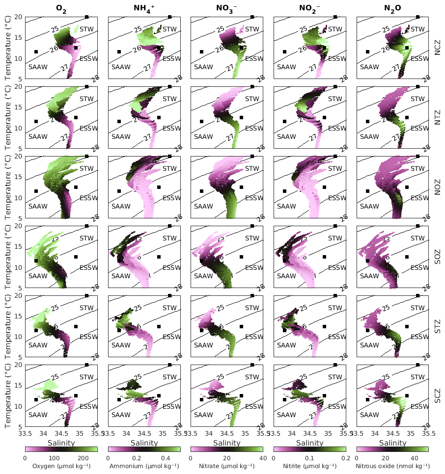
Figure 2 Diagram showing the averages of conservative temperature, absolute salinity, and biogeochemical tracers (in color) for the six study zones (see Fig. 1a). The biogeochemical tracers include oxygen (column 1), ammonium (column 2), nitrate (column 3), nitrite (column 4), and nitrous oxide (column 5). From top to bottom, the region names are: Northern Coastal Zone (NCZ); Northern Transition Zone (NTZ); Northern Oceanic Zone (NOZ); Southern Oceanic Zone (SOZ); Southern Transition Zone (STZ); and Southern Coastal Zone (SCZ). The zone selection is based on the characteristic water masses in the region, primarily the SAAW (Subantarctic Water) south of 30° S, whose biogeochemistry differs significantly from the STW (Subtropical Water) north of 30° S, particularly in oxygen, ammonium, and nitrite. The separation of the coastal, transitional, and oceanic zones considered the dominance of the ESSW in the subsurface waters and its oxygenation away from the coast.

The separation of coastal, transitional, and oceanic zones considered the dominance of Equatorial Subsurface Water (ESSW; 12.5 °C, 34.9) in the subsurface waters and its increasing oxygenation farther from the coast (Silva et al., 2009). Given the importance of ESSW in defining the study areas and in serving as the primary water source enclosed in the PUDDIES, the isopycnal surface associated with the ESSW and OMZ core was used as a reference. Specifically, we focused on the isopycnal with a density of 26.6 kg m⁻³, corresponding to the reference OMZ core in this model (Pizarro-Koch et al., 2019), which was used in part of our statistical analysis.

We thus came up with six subregions: Northern Coastal Zone (NCZ; suboxic conditions); Northern Transition Zone (NTZ; hypoxic conditions); Northern Oceanic Zone (NOZ; with 45 µM < O₂); Southern Oceanic Zone (SOZ; with 90 µM < O₂); Southern Transition Zone (STZ; with 45 µM < O₂<90 µM); and Southern Coastal Zone (SCZ; hypoxic conditions, Fig. 1a).

Within the first ∼100 km off the coast, the formation zone for PUDDIES was identified, where a large number of surface and subsurface eddies are typically generated (e.g., Chaigneau et al., 2009), as shown by the occurrence density of PUDDIES (Fig. 1b green strip). We considered the total number of PUDDY profiles with a grid box of approximately 1° by 1° in order to characterize the biogeochemical properties of the source water that the PUDDIES eventually enclose upon formation (see Sect. 2.6.1).

2.3 Definition of “mean state” and mesoscale contribution

To estimate the physical and biogeochemical perturbations from the mean field associated with the eddies, we used a Reynolds decomposition, which for the field of NO${}_{\mathrm{3}}^{-}$ concentration is written as follows in Eq. (2):

$$\begin{array}{}\text{(2)}& {\mathrm{NO}}_{\mathrm{3}}\left(x,y,z,t\right)=\langle {\mathrm{NO}}_{\mathrm{3}}{\rangle }_{\text{9-year}}+{{\mathrm{NO}}_{\mathrm{3}}}^{\prime }\left(x,y,z,t\right)\end{array}$$

where $\langle {\mathrm{NO}}_{\mathrm{3}}{\rangle }_{\text{9-year}}\left(x,y,z\right)$ is the “mean state” of NO${}_{\mathrm{3}}^{-}$ calculated as an overall mean across 9 years simulated between 2000 and 2008. Fluctuations of this “mean state” thus consider the large intraseasonal and seasonal variability and are denoted as ${{\mathrm{NO}}_{\mathrm{3}}}^{\prime }\left(x,y,z,t\right)$. Similarly, the other variables, 〈S〉_9-year, 〈NO₂〉_9-year, etc., denote the “mean state”, whereas S^′, NO${}_{\mathrm{2}}^{\prime }$, etc. correspond to anomalies, which include eddy fluctuations and changes associated with annual and interannual variability. The average anomalies were denoted as 〈S^′〉, $\langle {{\mathrm{NO}}_{\mathrm{2}}}^{\prime }\rangle$, etc. This decomposition method was used for all variables analyzed in each selected subregion (Fig. 1a). To evaluate the impacts of the PUDDIES on the various fields, we used an algorithm to identify subsurface eddies (see details in Sect. 2.5) and then compared the perturbed fields inside the PUDDIES with the total field. This latter procedure is further explained in Sect. 2.6.

2.4 Calculation of AOU, ΔNO${}_{\mathrm{3}}^{-}$, and ΔN₂O

The apparent oxygen utilization (AOU), NO${}_{\mathrm{3}}^{-}$ production (ΔNO${}_{\mathrm{3}}^{-}$), and N₂O production (ΔN₂O) provide an estimate of how much has been produced/consumed by biological processes since the water mass was formed in terms of oxygen, nitrate, and nitrous oxide, respectively. These estimates are associated with the time the water mass has spent without coming into contact with the ocean surface or being ventilated.

The AOU calculation was derived from the García and Gordon (1992) algorithm, based on the O₂ saturation concentration at any temperature and salinity:

$$\begin{array}{}\text{(3)}& \text{AOU}=[{\mathrm{O}}_{\mathrm{2}}{]}_{\mathrm{sat}}-[{\mathrm{O}}_{\mathrm{2}}]\end{array}$$

where [O₂]_sat is the oxygen saturation and was calculated based on Thermodynamic Equation of Seawater – 2010 (TEOS-10) (using the Gibbs-SeaWater Oceanographic toolbox) (https://www.teos-10.org/software.htm, last access: 18 August 2025); for [O₂], we used the modeled oxygen. The N₂O production (ΔN₂O) was calculated using the methodology of Gruber and Sarmiento (2002) and the following relationship, Eq. (4):

$$\begin{array}{}\text{(4)}& \mathrm{\Delta }{\mathrm{N}}_{\mathrm{2}}\mathrm{O}=\left[{\mathrm{N}}_{\mathrm{2}}\mathrm{O}\right]-[{\mathrm{N}}_{\mathrm{2}}\mathrm{O}{]}_{\mathrm{sat}}\end{array}$$

where [N₂O]_sat is the nitrous oxide saturation calculated from modeled temperature and salinity; for [N₂O], we used the modeled nitrous oxide. NO${}_{\mathrm{3}}^{-}$ production (ΔNO${}_{\mathrm{3}}^{-}$) is defined as follows,

$$\begin{array}{}\text{(5)}& \mathrm{\Delta }{\mathrm{NO}}_{\mathrm{3}}^{-}=\left[{\mathrm{NO}}_{\mathrm{3}}^{-}\right]-[{\mathrm{NO}}_{\mathrm{3}}^{-}{]}_{\mathrm{preformed}}\end{array}$$

where [NO${}_{\mathrm{3}}^{-}$] is the modeled nitrate. The value of [NO${}_{\mathrm{3}}^{-}$]_preformed in subsurface waters considered for the above calculation was that of the Equatorial Subsurface Water (ESSW), except in SOZ, where the value for Subantarctic Water (SAAW) was taken from Llanillo et al. (2012). The assessment of the modeled O₂, NO${}_{\mathrm{3}}^{-}$, and surface NO${}_{\mathrm{3}}^{-}$ is provided in Appendix A.

2.5 PUDDY identification

For the identification of PUDDIES, the algorithm proposed by Faghmous et al. (2014, 2015) was adapted to deal with subsurface eddies that have a weak dynamical signature at the surface of the ocean. The original algorithm is based on the presence of local extreme values of sea level anomalies (SLA) (minimum in the case of cyclonic eddies and maximum in the case of anticyclonic eddies, considering a neighborhood defined a priori around it). Because the SLA signal from subsurface eddies may be rather weak or absent, the present study used anomalies in the layer thickness (δh) defined as the difference between the depths of the density surfaces S_upper=26.0 kg m⁻³ and S_lower=26.9 kg m⁻³. Thus, positive anomalies (δh>0) indicate the presence of subsurface anticyclonic eddies due to their convex shape (for our case, PUDDIES). When δh is at its maximum (δh_max), the largest closed contour around the geographical location of δh_max is considered as the edge of the eddy, as δh_max is associated with the center of the eddy, and the points contained within the eddy edge are the body of the eddy (Fig. S2a; Faghmous et al., 2015). Starting from δh_max, a gradual decrease of 0.1 m was used to establish the size and amplitude of the eddy. Only eddies that reached a minimum horizontal area of 30 grid points ($A_{\min }\sim \mathrm{1.95}\times {\mathrm{10}}^{\mathrm{9}}$ m², equivalent to a radius of ∼25 km) were considered, as eddies below this threshold are not well identified (reducing the total of selected PUDDIES by 30 %). Additionally, only eddies with a radius not exceeding 150 km (∼32 pixels in diameter) were included, as larger eddies are also not well detected, with at most three closed-contour structures per snapshot being discarded. This also helps distinguish eddies in coastal regions from other processes, such as coastal trapped waves or upwelling events, which occur on larger spatial scales.

Eddy identification was performed using 3 d averages across the entire period. Subsequently, all δh_max positions were classified by subregion and in 1° × 1 ° cells for their enumeration (Fig. 1b) and for characterizing the average properties of these PUDDIES along the coast (see Sect. 2.6.1; statistical analyses are shown in Sect. 3).

2.6 Compound formation

2.6.1 Average PUDDY profiles

To understand the typical conditions within PUDDIES identified in the formation zone and each subregion, average profiles were constructed as follows: (i) all eddy centers (i.e., δh_max positions) were classified in 1° × 1° grid cells along the coast and also within the regions defined in Fig. 1a, (ii) for each eddy center, vertical profiles were extracted between the density surfaces S_upper and S_lower for all variables, in each corresponding region, (iii) then, these profiles were time-averaged to obtain typical profiles for each variable. For the different regions, the values associated with the S_core are shown (Sect. 3.2) to emphasize changes in the ESSW core. The analysis of these results is presented in Sect. 3.1 and 3.2.

2.6.2 Average zonal compound

Based on the identification of eddies over a 9-year period, different latitude bands (25, 30, and 36° S, Fig. 1a) were selected to create a composite constructed from 3D PUDDIES, considering all the δh_max values identified within 1° × 1° areas. For these PUDDIES, we estimated characteristics within the entire eddy volume as follows: (i) for each δh_max (PUDDY center), a mask of the entire volume was created; (ii) the area mask was calculated to identify the edge using Faghmous et al.'s (2014, 2015) algorithm, which was found to be the most accurate approach (Fig. S3; see sensitivity analysis in the Supplement); (iii) this mask was applied across all depths (at 5 m intervals), creating an irregular cylinder between S_upper and S_lower; (iv) from the total volume enclosed by the cylinder, an average vertical profile was obtained at each time step for each variable (see an example of vertical PUDDY characterization in Fig. S2b–e).

A total of 862 PUDDIES (δh_max values) were accounted for in the 25° S zonal band, 810 in the 30° S band, and 658 in the 36° S band. Additionally, for each latitude, biogeochemical variables averaged over the 9-year period, representing the mean state (defined in Sect. 2.3), were used to calculate an average profile associated with a 1° × 1° area. Anomalies were then calculated as the difference between these two profiles. The results of this statistical analysis and the subsurface modifications caused by PUDDIES are presented in Sect. 3.4.

2.7 Calculation of percentiles

To assess the significance of the internal contribution of PUDDIES relative to the mean state (defined in Sect. 2.3), we employed a bootstrap method, which involved randomly sampling more than 200 positions in each region and deriving diagnostics. A total of 92 random time steps were selected, and for each time step, 1000 latitudes and 1000 longitudes were generated within the domain. These positions were then filtered for each region. The total number of random positions found per region was as follows: 1246 in NCZ, 1474 in NTZ, 3509 in NOZ, 6808 in SOZ, 521 in STZ, and 235 in SCZ (Table S2).

For each obtained position, the biogeochemical properties were extracted at the S_core. This approach generated an ensemble of values, allowing us to infer the 50th, 75th, and 90th percentiles (P50, P75, P90), used to provide an estimate of significance levels.

3 Results

3.1 Contrasting biogeochemical characteristics inside and outside the PUDDIES in the formation zone

The region within the first ∼100 km off the coast was considered a formation zone for PUDDIES where a large number of surface and subsurface eddies are typically generated (e.g., Chaigneau et al., 2009; Fig. 1b, green strip). Approximately 1° of latitude × 1° longitude boxes were selected along the coast to characterize the biogeochemical properties of the source water that the PUDDIES eventually enclose upon formation (see Sect. 2.6.1).

Over the 9-year study period in the simulated study region (Fig. 1a), an average of approximately 14 PUDDIES was observed at each time step, resulting in a total of ∼15 340 PUDDY profiles (defined as the vertical profile associated with the δh_max) identified (see Sect. 2.5). If the same eddy remained within the same 1° × 1° grid area, it was counted multiple times (using a 3 d time step) until the center of the eddy moved to an adjacent 1° × 1° grid. The area with the highest density of identified PUDDY profiles was concentrated in the coastal region (2548), within the first ∼100 km from shore, with the maximum abundance noted between 29 and 35° S (Fig. 1b). To assess the impact of PUDDIES along the coastal strip, we evaluated the mean distribution of several variables (salinity, O₂, NO${}_{\mathrm{3}}^{-}$, NO${}_{\mathrm{2}}^{-}$, NH${}_{\mathrm{4}}^{+}$, and N₂O) in areas of approximately 1° × 1° along the coast from 20 to 38° S and between the isopycnal surfaces S_upper and S_lower that define the OMZ core in the model (see details in Sect. 2.6.1). Then, we calculated the mean profiles of these variables in the center of the PUDDIES observed in each discrete coastal area (1° × 1°) and estimated anomalies of the profiles relative to the general mean profile of the corresponding box (Fig. 3, see also Fig. S4 in the Supplement).

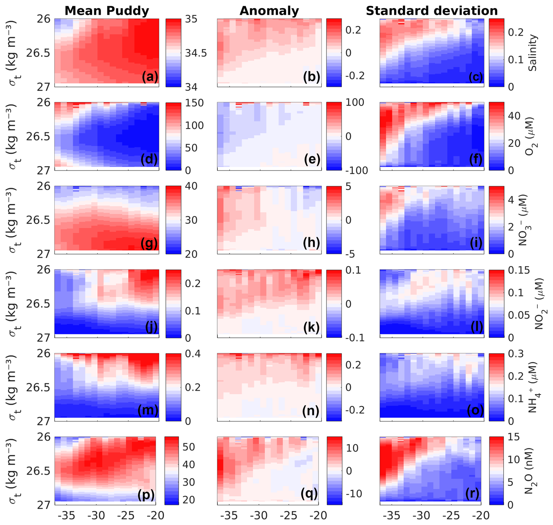
Figure 3 Composite mean vertical profiles (left column), their anomalies relative to the long-term mean (middle column), and the standard deviation of the anomalies (right column) associated with biogeochemical features within the center of the PUDDIES over the first ∼100 km from the slope where there are higher occurrence of PUDDIES (strip in green in Fig. 1b). From top to bottom: (a–c) absolute salinity (g kg⁻¹), (d–f) O₂, (g–i) NO${}_{\mathrm{3}}^{-}$, (j–l) NO${}_{\mathrm{2}}^{-}$, (m–o) NH${}_{\mathrm{4}}^{+}$, and (p–r) N₂O. Eddy mean profiles were obtained by calculating the mean of total profiles identified during nine years in 1° × 1° boxes along the coast between the isopycnal layers S_upper and S_lower (see Sect. 2.6.1). The standard deviation is interpreted as the variability of the properties existing at the center. The x axis represents the latitude in degrees, and the y axis shows the potential density anomaly.

Meridional changes in water properties along the coastal strip impact the initial properties of the PUDDIES. In the northern sector (between 20 and 30° S), the waters are warmer and more saline and have lower O₂ (Fig. 3a, d), with higher concentrations of NO${}_{\mathrm{2}}^{-}$ and NH${}_{\mathrm{4}}^{+}$ (Fig. 3j and m). In contrast, toward the south (south of 30° S), these characteristics generally show the opposite tendency, consistent with the water properties observed within PUDDY cores. However, NO${}_{\mathrm{3}}^{-}$ and N₂O exhibit maximum levels in the central region (near 30° S) (Fig. 3g and p), where eddies with the highest N₂O concentrations are also observed. Oxygen levels were higher at the upper and lower limits of the OMZ (i.e., near σ_θ=26.3 kg m⁻³ and σ_θ=26.7 kg m⁻³) and remained relatively low in the OMZ core (σ_θ∼26.5 kg m⁻³). Both NH${}_{\mathrm{4}}^{+}$ and NO${}_{\mathrm{2}}^{-}$ anomalies generated by the PUDDIES showed maximum values in the upper limit of the eddy cores (near σ_θ=26.3 kg m⁻³; Fig. 3k, n) and were fairly uniform along the coastal strip, except between 22 and 24° S and the north-central region, which showed slightly higher anomalies (Fig. 3k). South of 33° S, in the narrowest part of the OMZ, the largest anomalies in O₂, NO${}_{\mathrm{3}}^{-}$, and N₂O are observed (Fig. 3e, h, q), accompanied by a higher standard deviation (Fig. 3f, i, r).

Table 1 General characteristics of the study subregions. The S_upper layer refers to σ_θ=26.0 kg m⁻³, the S_core layer refers to σ_θ=26.6 kg m⁻³, and the S_lower layer corresponds to σ_θ=26.9 kg m⁻³. Their average depth is indicated, with (±) indication of the errors estimated based on a bootstrap method (see Sect. 2). Mean thickness was defined as the distance between the S_upper and S_lower isopycnal layers.

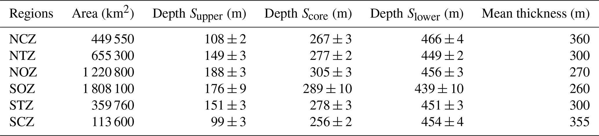
Table 2 Linear regression between average AOU (µM, 〈AOU〉_9-year) and average salinity (g kg⁻¹, 〈S〉_9-year) and between average oxygen (µM, 〈O₂〉_9-year) and 〈S〉_9-year within each subregion in the S_core layer (σ_θ=26.6 kg m⁻³). Linear correlation coefficient (R²) provides a measure of how well 〈AOU〉_9-year and 〈O₂〉_9-year are accounted for by a linear model where mean absolute salinity is considered a predictor. Errors in the parameter estimates are provided.

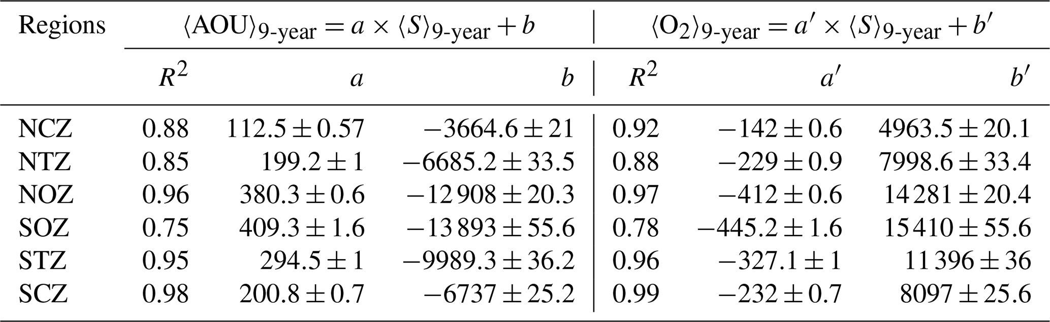
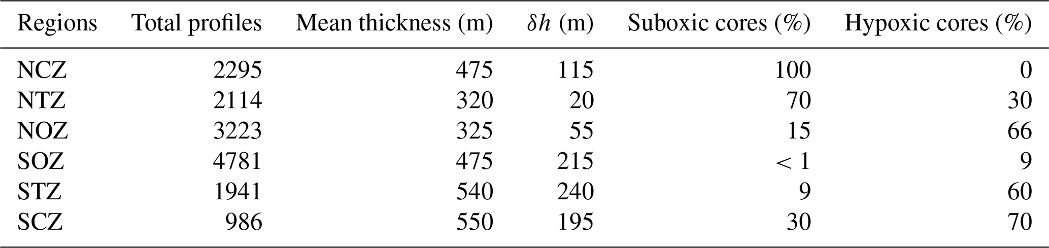
Table 3 Percentage of total identified PUDDIES showing suboxic (O₂<20 µM) and hypoxic (20 µM < O₂<45 µM) cores within each region. Total profiles indicate the PUDDY profiles identified over the entire study period. Mean thickness shows the distance between S_upper (σ_θ=26.0 kg m⁻³) and S_lower (σ_θ=26.9 kg m⁻³), and δh is the average anomaly thickness generated due to the passage of PUDDIES in that region (i.e., composite δh anomaly).

3.2 Biogeochemical characteristics inside the offshore PUDDIES

From the total of 15 340 PUDDY profiles, statistics over the six subregions defined in Sect. 2.2 (see also Fig. 1a) were performed. These results are synthesized in Tables 1 to 3. Table 1 provides statistics associated with general characteristics of the subregion, Table 2 presents statistics on ESSW properties, while Table 3 focuses on PUDDIES' characteristics.

3.2.1 Oxygen and salinity relationship in ESSW

An evaluation of the relationship between average salinity (〈S〉_9-year, as a conservative variable), average oxygen (〈O₂〉_9-year), and average AOU (〈AOU〉_9-year) was conducted for each subregion (Table 2). This analysis was performed using the isopycnal with a density of 26.6 kg m⁻³, where the ESSW core was observed (see Sect. 2.2).

Each water mass acquires characteristics through physical and biogeochemical processes, producing particular relationships between the physicochemical variables. Low O₂ waters are closely related to relatively salty ESSW waters. In our study region, this water mass is located between two low-salinity and relatively well-ventilated water masses (i.e., SAAW above and Antarctic Intermediate Water (AAIW) below). Thus, salinity and O₂ show a linear inverse correlation between the upper and lower oxyclines that delimit the OMZ. Nevertheless, the occurrence of biogeochemical processes can disrupt this relationship. Therefore, it is useful to quantify which regions show these nonlinear biogeochemical processes in the context of the hypothesis that a linear relationship between O₂ and salinity corresponds to an aging of the water mass due to a lack of ventilation. A nonlinear relationship would imply the presence of other processes, such as denitrification. Linear regression was performed between absolute salinity, O₂, and AOU on the S_core surface, where AOU provides a measure of the apparent O₂ consumption since the ESSW formation (Table 2).

Oxygen and AOU exhibited a strong linear relationship with absolute salinity (R²>0.85) in regions where there is a greater contribution from ESSW (NCZ, NTZ, NOZ, STZ, and SCZ). The slope values ranged from 112.5 to 380 for AOU and 142 to 412 for O₂ fit. In contrast, the SOZ exhibited a weaker linear relationship (R²<0.80), likely due to the mixing properties of SAAW and AAIW with ESSW (Fig. 2, Table S1). SCZ (R²>0.98) showed the strongest relationship in the coastal zone, which decreased in NCZ (R²<0.96), where denitrification processes have been recorded and there are evident high values of AOU and nitrate deficiency (Fig. 4a, b; Tables 2 and S1). In the northern region, the linear fit improves as it approaches the oceanic zone (NOZ) (R²>0.96), indicating a strong presence of the ESSW and a reduced influence from either this biological process or mixing with another water mass.

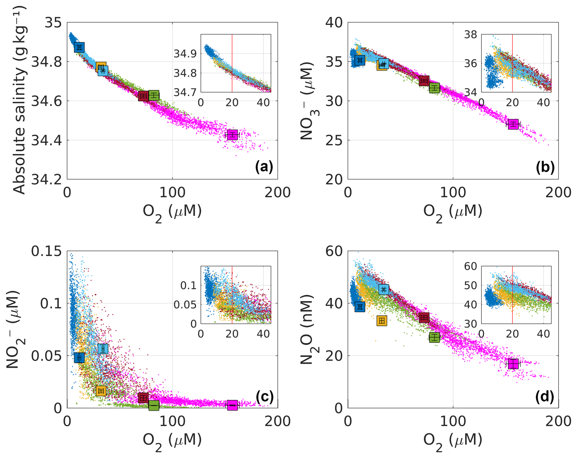
Figure 4 Relationship between mean O₂ concentration and (a) absolute salinity, (b) NO${}_{\mathrm{3}}^{-}$, (c) NO${}_{\mathrm{2}}^{-}$, and (d) N₂O at the S_core layer for all identified PUDDIES. The dots represent the core properties of all PUDDIES (in the S_core) identified over a 9-year period, at each time step. The color indicates the subregion (see Sect. 2.6.1), which was compared to the mean state value (colored squares, Sect. 2.3). A positive oxygen gradient is observed from coastal regions (NCZ – dark blue; SCZ – light blue), followed by transition zones (NTZ – yellow; STZ – brown) to the oceanic regions (NOZ – green; SOZ – magenta). Error bars inside the squares correspond to the standard deviation of biogeochemical values within the S_core for each subregion. The smaller box shows a magnified view of the larger box to highlight hypoxic (20 µM < O₂<45 µM) and suboxic (1 µM < O₂<20 µM) conditions. The red line indicates the threshold of O₂=20 µM.

3.2.2 Conditions of suboxia and hypoxia in the oceanic PUDDIES

We assessed the number of PUDDIES exhibiting suboxia and hypoxia in each region by identifying the predominant type of low-oxygen cores in coastal, transition, and oceanic zones. The main results are presented in Table 3. The percentage of PUDDIES exhibiting hypoxia (O₂<45 µM) and suboxia (O₂<20 µM) was determined by classifying the range of O₂ concentrations observed in the center of the eddies. The presence of PUDDIES with these characteristics in the more remote regions was quantified (referred to as NOZ and SOZ in Table 3).

3.2.3 Differences between biogeochemical properties inside and outside PUDDIES

To understand the biogeochemical impacts of eddies in oceanic waters, the tracer values found in the core of the PUDDIES were compared with the “mean conditions” (Fig. S5) of each region in S_core. The presence of PUDDIES manifests a physical change in the mean thickness through the perturbation of isopycnal layers during the passage of PUDDIES, which appears as the average anomaly thickness (δh), different in each subregion (Table 3), and biogeochemical changes with greater contrast observed away from the coast in the south (Fig. 4). Values of 〈AOU^′〉, $\langle \mathrm{\Delta }{{\mathrm{NO}}_{\mathrm{3}}}^{\prime }\rangle$, and $\langle \mathrm{\Delta }{{\mathrm{N}}_{\mathrm{2}}\mathrm{O}}^{\prime }\rangle$ observed inside the PUDDIES were higher than 〈AOU〉_9-year, 〈ΔNO₃〉_9-year, and 〈ΔN₂O〉_9-year observed outside (Figs. 4, 5, 6; Table S1, S2), confirming that eddies maintain hypoxic or suboxic cores that impact regions farther offshore, as shown in Sect. 3.2.2 (Table 3).

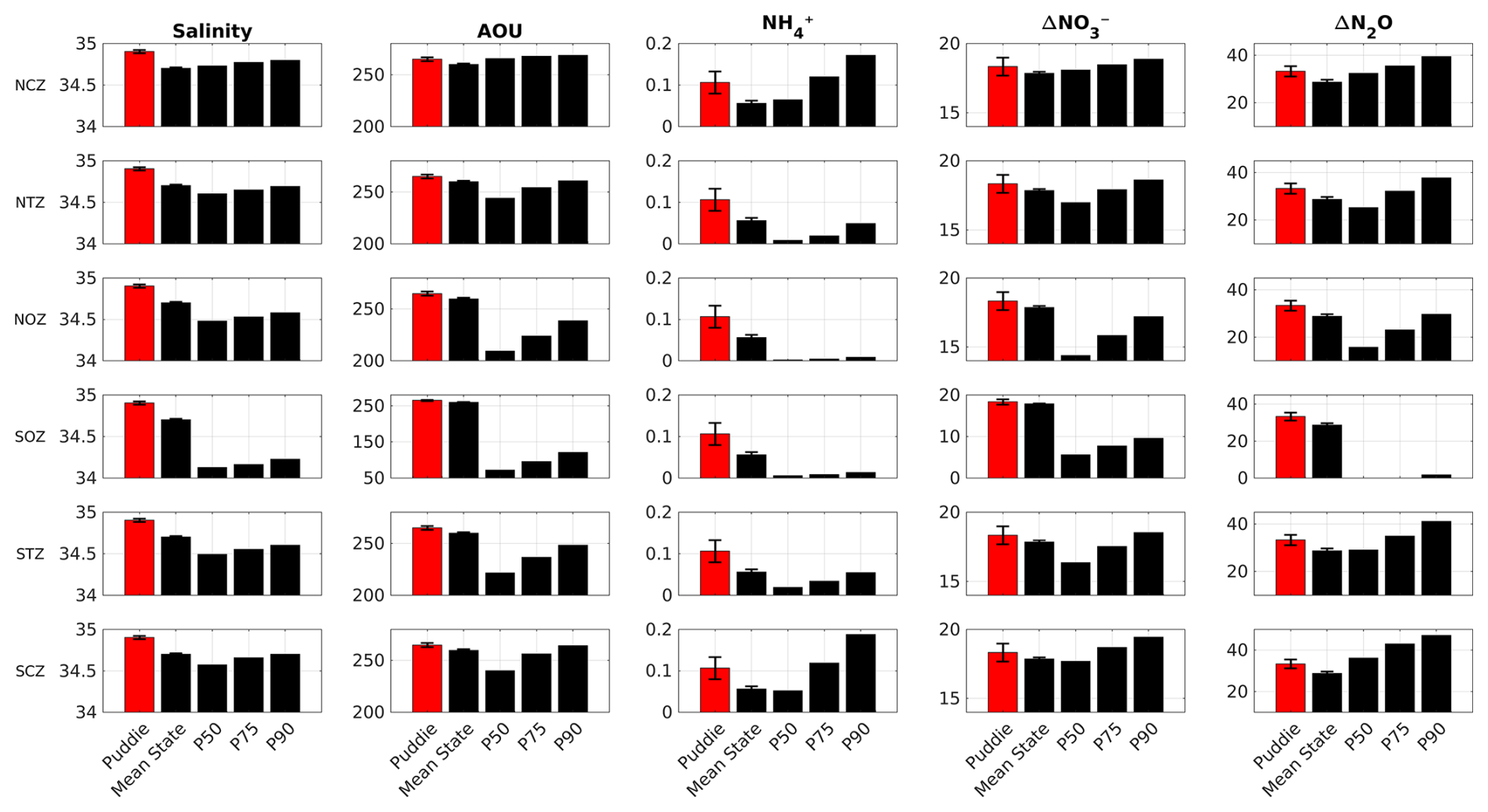
Figure 5 Comparison between the average value associated with all PUDDIES (red color), the mean state, and the 50th, 75th, and 90th percentiles (black color, P50, P75, P90, respectively) for absolute salinity (g kg⁻¹), AOU, NH${}_{\mathrm{4}}^{+}$, ΔNO${}_{\mathrm{3}}^{-}$ (µM), and ΔN₂O (nM) in each region (see Sect. 2.4). The profiles for calculating the percentiles are based on a distribution between 235 and 6800 values – according to the size of the region – obtained from random resampling using Monte Carlo's method (see Sect. 2.7). The averages were calculated for the S_core layer (see Sect. 2). The error bars indicate the standard deviation for PUDDIES and for the mean state (see also Tables S1 and S2 for complementary information).

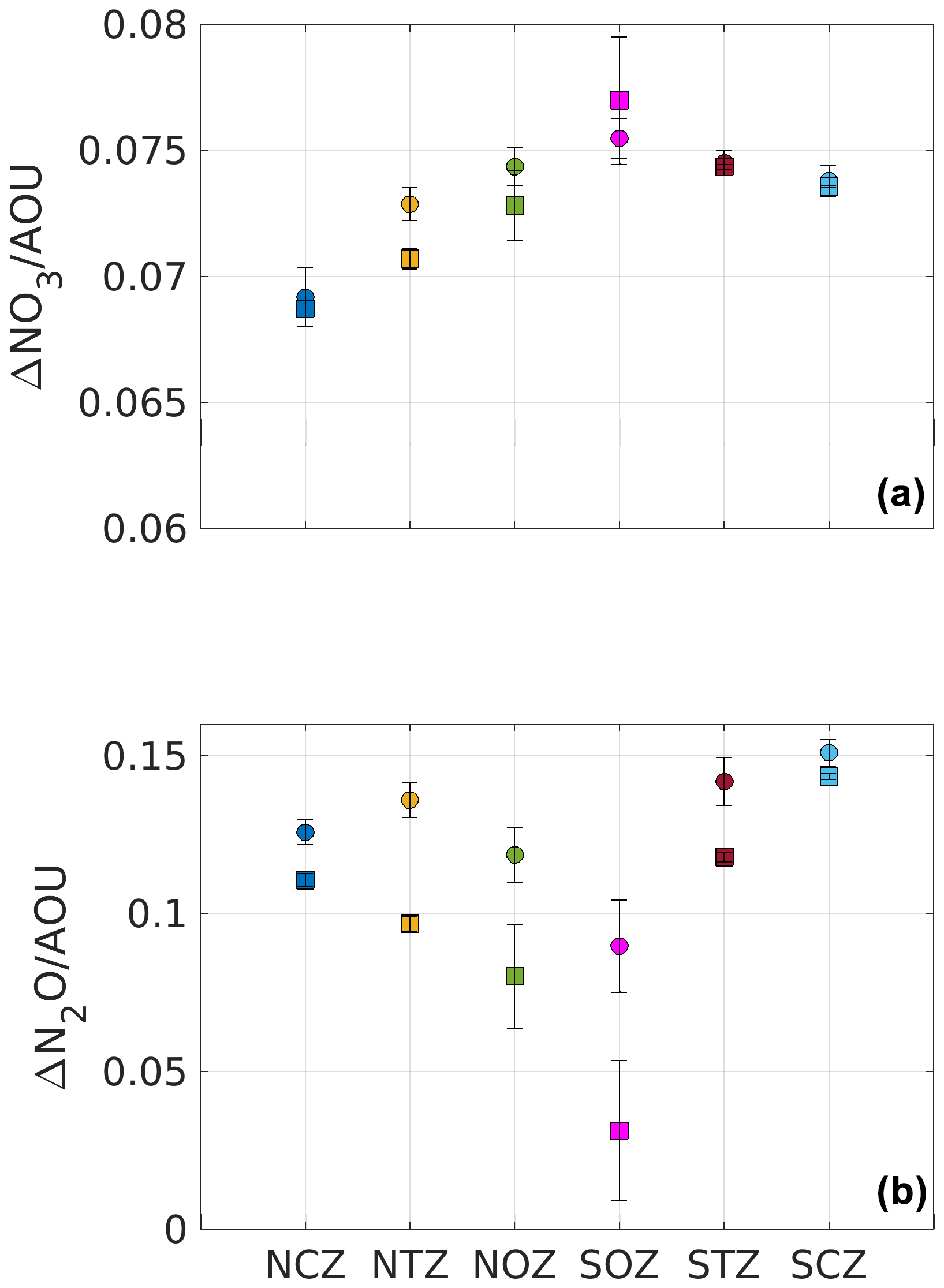
Figure 6 Mean ratios for composite PUDDIES and mean conditions within each region. (a) Ratios of ΔNO${}_{\mathrm{3}}^{-}/\text{AOU}$. Note that values are smaller than the Redfield ratio ($R_{\mathrm{N}/\mathrm{O}}=\mathrm{0.11}$). (b) Ratios of $\mathrm{\Delta }{\mathrm{N}}_{\mathrm{2}}\mathrm{O}/\text{AOU}$. Values of composite PUDDIES are indicated with circles, while values of the mean state conditions are indicated with squares. Values are for the S_core layer (see Sect. 2). Color code is similar to that of Fig. 4. The error bar indicates half the standard deviation calculated from the relationship between $\mathrm{\Delta }{\mathrm{NO}}_{\mathrm{3}}^{-}/\text{AOU}$ and $\mathrm{\Delta }{\mathrm{N}}_{\mathrm{2}}\mathrm{O}/\text{AOU}$ within the S_core for each subregion.

On the other hand, the asymptotic behavior of NO${}_{\mathrm{2}}^{-}$ was similar to that of NH${}_{\mathrm{4}}^{+}$ (not shown), occurring when O₂<45 µM (NCZ, NTZ, and SCZ) and tending toward undetectability in regions where O₂>45 µM (Fig. 4c). In SCZ, PUDDIES with higher concentrations of N₂O than in NCZ (which has suboxic conditions) and NTZ (with hypoxic conditions) can be observed (Fig. 4d, Table S1).

In general, in the NCZ and SCZ, PUDDIES maintain the same average salinity, exhibiting an increment of 0.5–0.7 µM ΔNO${}_{\mathrm{3}}^{-}$ (+2.5 %–4 %), 0.01–0.05 µM NH${}_{\mathrm{4}}^{+}$ similar to NO${}_{\mathrm{2}}^{-}$ (+12.5 %–83 %), and 3–4.5 nM ΔN₂O (+9 %–16 %) associated with an increase of 5–9 µM AOU (+2 %–4 %) higher than the mean state (Figs. 4 and 5; more details, see Table S1). These anomalies were greater than the 50th percentile (P50) for ΔNO${}_{\mathrm{3}}^{-}$ and ΔN₂O and close to the 75th percentile (P75) for AOU and NH${}_{\mathrm{4}}^{+}$ with salinity exceeding P90 (Fig. 5), indicating a significant elevation of biogeochemical elements in the coastal zones due to PUDDIES compared to the mean state. Offshore, the contrast with the mean state was greater, particularly in the SOZ, reaching 100 % for NH${}_{\mathrm{4}}^{+}$, 43 % for ΔNO${}_{\mathrm{3}}^{-}$, 215 % for ΔN₂O, 45 % for AOU, and 0.3 g kg⁻¹ for salinity. These values exceed the P90 (Table S2). Similarly, in the NOZ and STZ, only NH${}_{\mathrm{4}}^{+}$ exceeded P90, while the rest remained at P75. In NTZ, the AOU and ΔN₂O had values close to or greater than P75, while NH${}_{\mathrm{4}}^{+}$ and ΔNO${}_{\mathrm{3}}^{-}$ exceeded P90 (Fig. 5). The perturbations to the mean state contributed by PUDDIES in the open sea are more significant than near the coast, although salinity and biogeochemical tracers decrease as the core becomes more oxygenated offshore.

The AOU $/$ ΔNO${}_{\mathrm{3}}^{-}$ ratio allows us to quantify the remineralization of organic matter through aerobic processes, which is determined by the Redfield ratio ($R_{\mathrm{N}/\mathrm{O}}$; $\mathrm{16}/\mathrm{138}=\mathrm{0.11}$; Redfield et al., 1963). Changes in this relationship indicate the presence of other biological processes that contribute/consume nitrogen in a system, such as nitrogen fixation ($\mathrm{\Delta }{\mathrm{NO}}_{\mathrm{3}}^{-}/\text{AOU}>R_{\mathrm{N}/\mathrm{O}}$) and denitrification ($\mathrm{\Delta }{\mathrm{NO}}_{\mathrm{3}}^{-}/\text{AOU}<R_{\mathrm{N}/\mathrm{O}}$). On the other hand, the $\mathrm{\Delta }{\mathrm{N}}_{\mathrm{2}}\mathrm{O}/\text{AOU}$ ratio provides a measure of N₂O accumulation, so that a high $\mathrm{\Delta }{\mathrm{N}}_{\mathrm{2}}\mathrm{O}/\text{AOU}$ is associated with the denitrification process (Sarmiento and Gruber, 2006).

We observed a $\mathrm{\Delta }{\mathrm{NO}}_{\mathrm{3}}^{-}/\text{AOU}$ ratio lower than $R_{\mathrm{N}/\mathrm{O}}$, inside and outside the PUDDIES (Fig. 6, upper box), indicating a deficit of NO${}_{\mathrm{3}}^{-}$ and high O₂ consumption due to the elevated remineralization in subsurface waters. The ratio is higher in the suboxic region (NCZ) with an AOU : ΔNO${}_{\mathrm{3}}^{-}=\mathrm{15}:\mathrm{1}$, while in the other regions this signal of old and poorly ventilated waters also extends, albeit in different proportions (Table S1). When $\frac{\langle \mathrm{\Delta }{{\mathrm{NO}}_{\mathrm{3}}}^{\prime }\rangle }{\langle {\text{AOU}}^{\prime }\rangle }<\frac{\langle \mathrm{\Delta }{\mathrm{NO}}_{\mathrm{3}}{\rangle }_{\text{9-year}}}{\langle \text{AOU}{\rangle }_{\text{9-year}}}$, it must be the case that 〈AOU^′〉 is greater than 〈AOU〉_9-year or $\langle \mathrm{\Delta }{{\mathrm{NO}}_{\mathrm{3}}}^{\prime }\rangle$ is less than 〈ΔNO₃〉_9-year. Since the second assumption is not met, it is true that 〈AOU^′〉 is greater than 〈AOU〉_9-year (Table S1). However, in regions NTZ and NOZ, $\frac{\langle \mathrm{\Delta }{{\mathrm{NO}}_{\mathrm{3}}}^{\prime }\rangle }{\langle {\text{AOU}}^{\prime }\rangle }>\frac{\langle \mathrm{\Delta }{\mathrm{NO}}_{\mathrm{3}}{\rangle }_{\text{9-year}}}{\langle \text{AOU}{\rangle }_{\text{9-year}}}$, indicating that $\langle \mathrm{\Delta }{{\mathrm{NO}}_{\mathrm{3}}}^{\prime }\rangle$ is greater than 〈ΔNO₃〉_9-year or 〈AOU^′〉 is less than 〈AOU〉_9-year. Given that 〈AOU^′〉 is greater than 〈AOU〉_9-year, it must be that $\langle \mathrm{\Delta }{{\mathrm{NO}}_{\mathrm{3}}}^{\prime }\rangle$ is greater than 〈ΔNO₃〉_9-year, so the production of NO${}_{\mathrm{3}}^{-}$ was greater in the PUDDIES found in these regions compared to others (Table S1). On the other hand, it holds that $\frac{\langle \mathrm{\Delta }{{\mathrm{N}}_{\mathrm{2}}\mathrm{O}}^{\prime }\rangle }{\langle {\text{AOU}}^{\prime }\rangle }>\frac{\langle \mathrm{\Delta }{\mathrm{N}}_{\mathrm{2}}\mathrm{O}{\rangle }_{\text{9-year}}}{\langle \text{AOU}{\rangle }_{\text{9-year}}}$. Since 〈AOU^′〉 is greater than 〈AOU〉_9-year, it also follows that $\langle \mathrm{\Delta }{{\mathrm{N}}_{\mathrm{2}}\mathrm{O}}^{\prime }\rangle$ is greater than 〈ΔN₂O〉_9-year, and therefore the production of N₂O was proportionally larger than O₂ consumption in the PUDDIES (Fig. 6, lower box; Table S1). Note that although in SCZ and STZ the eddies exhibited the highest values of $\frac{\langle \mathrm{\Delta }{{\mathrm{N}}_{\mathrm{2}}\mathrm{O}}^{\prime }\rangle }{\langle {\text{AOU}}^{\prime }\rangle }$, $\frac{\langle \mathrm{\Delta }{\mathrm{N}}_{\mathrm{2}}\mathrm{O}{\rangle }_{\text{9-year}}}{\langle \text{AOU}{\rangle }_{\text{9-year}}}$ was also high (Fig. 6). Additionally, the variability of physicochemical conditions in the core increased with distance from the coast and oxygenation.

To sum up, according to our model results, PUDDIES generate significant changes in the mean conditions observed in all regions; particularly large differences were found in AOU and ΔN₂O in SOZ. In contrast, the differences in ΔNO${}_{\mathrm{3}}^{-}$ and AOU were not significant in the coastal regions (NCZ and SCZ).

3.3 Oxygen budget in the PUDDIES

The processes that contribute to the modulation of the total O₂ content are represented in the advection–diffusion equation (Eq. 1, Sect. 2.1). One part of the equation is associated with O₂ changes due to physical processes (referred to as PHYS), and another part is related to the production/consumption of O₂ through biogeochemical processes (SMS), so we can write $\frac{\partial {\mathrm{O}}_{\mathrm{2}}}{\partial t}=\text{PHYS}+\text{SMS}$. PHYS comprises horizontal advective processes (HADV = XADV + YADV), horizontal mixing (HMIX) in the x–y plane, vertical advection (VADV), and vertical mixing (VMIX) in the z direction so that PHYS = HADV + VADV + HMIX + VMIX. Note that HMIX and VMIX are mainly related to small-scale (subgrid-scale processes) mixing (e.g., Pizarro-Koch et al., 2019). On the other hand, the SMS (source minus sink processes of O₂) includes primary production, remineralization, nitrification, and zooplankton excretion (SMS = PP + Rem + Nitrif + Exc).

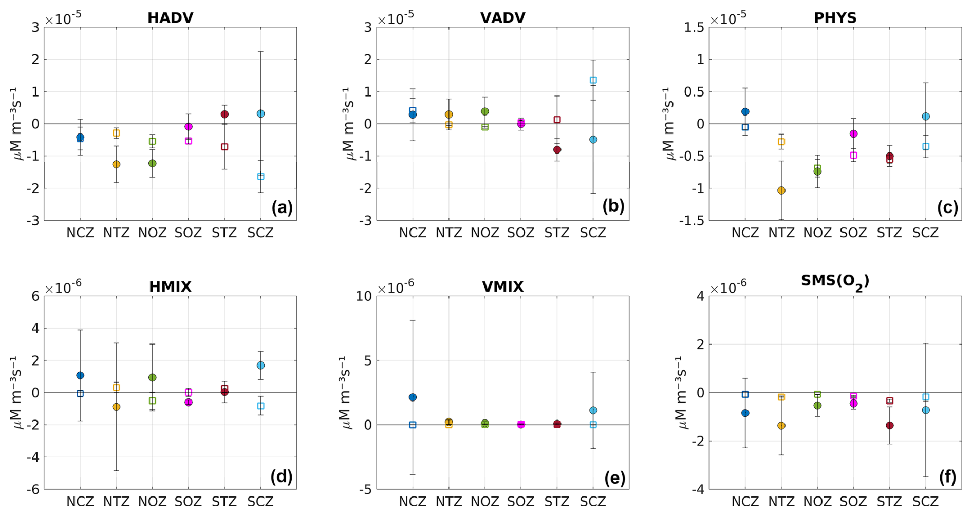
Figure 7 Mean terms involved in the O₂ budget (see Eq. 1). The different terms were temporally averaged inside the eddies in each subregion. PHYS is the sum of physical processes, which encompass horizontal advection (HADV = XADV + YADV), vertical advection (VADV), horizontal mixing (HMIX), and vertical mixing (VMIX). The biogeochemical processes are included as source minus sink (SMS) processes impacting O₂. In particular, SMS includes the O₂ fluxes from primary production, nitrification, remineralization, and zooplankton excretion. Positive (negative) values indicate processes contributing to increasing (depleting) O₂ inside the eddy. (a) HADV, (b) VADV, (c) PHYS, (d) HMIX, (e) VMIX, and (f) SMS. The averaging was carried out by dividing the composite PUDDY profile (see Sect. 2.6.1) into two parts: above (fill circles) and below (squares) the 26.5 kg m⁻³ isopycnal surface. This division was based on the marked vertical variability observed in the probability density function, as indicated by the variance and skewness (Fig. S6). The vertical bars represent standard deviations of the O₂ budget terms within S_core for each subregion.

We analyzed the contribution of each component of the equation to the O₂ balance in the center of the PUDDIES, dividing the contributions above and below the S_core (Fig. 7). This was motivated by the fact that there is a significant variance in the upper part of the eddy cores, which is also associated with a large skewness (Fig. S6). This indicates a marked vertical variability in the probability density function of the different terms involved in the O₂ balance in the upper part of the eddy cores, probably induced by vertical mixing. Positive (negative) values indicate O₂ increase/production (decrease/consumption). In general, we observed that the contribution of PHYS was negative, mainly in the lower part of the eddy, while only in NCZ and SCZ did positive values dominate at the top, although they were weak, indicating O₂ increase within the core (Fig. 7c). On the other hand, O₂ consumption through SMS (maximum in the transition zones NTZ and STZ) occurred in the upper part of the PUDDIES (Fig. 7f). This proves that elevated biological activity is maintained in the eddies far from shore, with higher intensity in younger eddies but weakening in eddies that reach regions very distant from the coast (NOZ and SOZ). Although the SMS fluxes are of the order O(10⁻⁶), 1 order of magnitude lower than the PHYS, small changes in O₂ due to SMS can also result in a sharp local spatial gradient in O₂ that induces strong changes in the advection of O₂. This could significantly impact the behavior of biogeochemical components that are highly sensitive to minimal changes in O₂ concentration, especially under hypoxic or suboxic conditions.

The advection components (O(10⁻⁵)) can be interpreted as the ability to maintain O₂ at the center of the eddy during the eddy's displacement. They dominate the O₂ budget compared to mixing processes (O(10⁻⁶)) involving diffusion of O₂ (Fig. 7a, b). The lateral fluxes (HADV) showed O₂ leakage (HADV <0) from the core mainly in the northern eddies but not in the southern eddies (HADV >0), where O₂ influx to the core was evident (Fig. 7a). Assuming vertical oxygen advection dominates over shear-induced oxygen transport, in the northern regions, VADV >0 dominates in the upper part of the PUDDIES, indicating O₂ input. In contrast, in the southern regions, this pattern is reversed. In coastal zones, vertical advective processes become significant, with VADV >0, highlighting the greater O₂ input in SCZ (Fig. 7b).

Vertical mixing fluxes were positive in newly formed eddies (mainly in coastal regions), while lateral diffusion fluxes showed high variability in magnitude and direction (Fig. 7d, e).

3.4 Subsurface water band changes by PUDDIES

In this section, a robust approach was used to demonstrate the effect of PUDDIES on the mean state through the modification of biogeochemical properties, vertical structure, and the contribution of various processes to changes in the subsurface water band delimited by the density surfaces S_upper and S_lower across different latitudes (25, 30, and 36° S) during their interaction. All PUDDIES identified in the three latitudinal bands over the 9-year period were used to build a composite by extracting properties in x–y–z dimensions to obtain the average zonal variables associated with PUDDIES (details in Sect. 2.6.2).

Table 4 Estimates of the decay rate of tracers along 25, 30, and 36° S for the mean state and anomalous conditions within PUDDIES. The decay rate is derived from an exponential fit of the form $y=A{e}^{-kx}$, where x represents the distance from the coast in km and y is the concentration of the biogeochemical tracer. k is the decay rate, and A represents the tracer concentration in the coastal strip (1° × 1°). A zonal extent of 1445 km was used at 25 and 30° S, while at 36° S, we used 1334 km (i.e., the same range of longitude as in Fig. 8). Values of k are statistically significant at the 95 % confidence level.

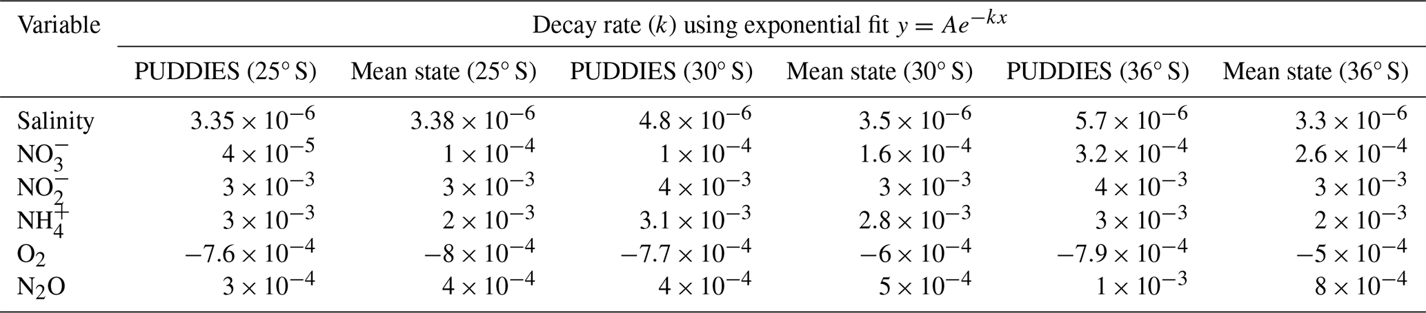
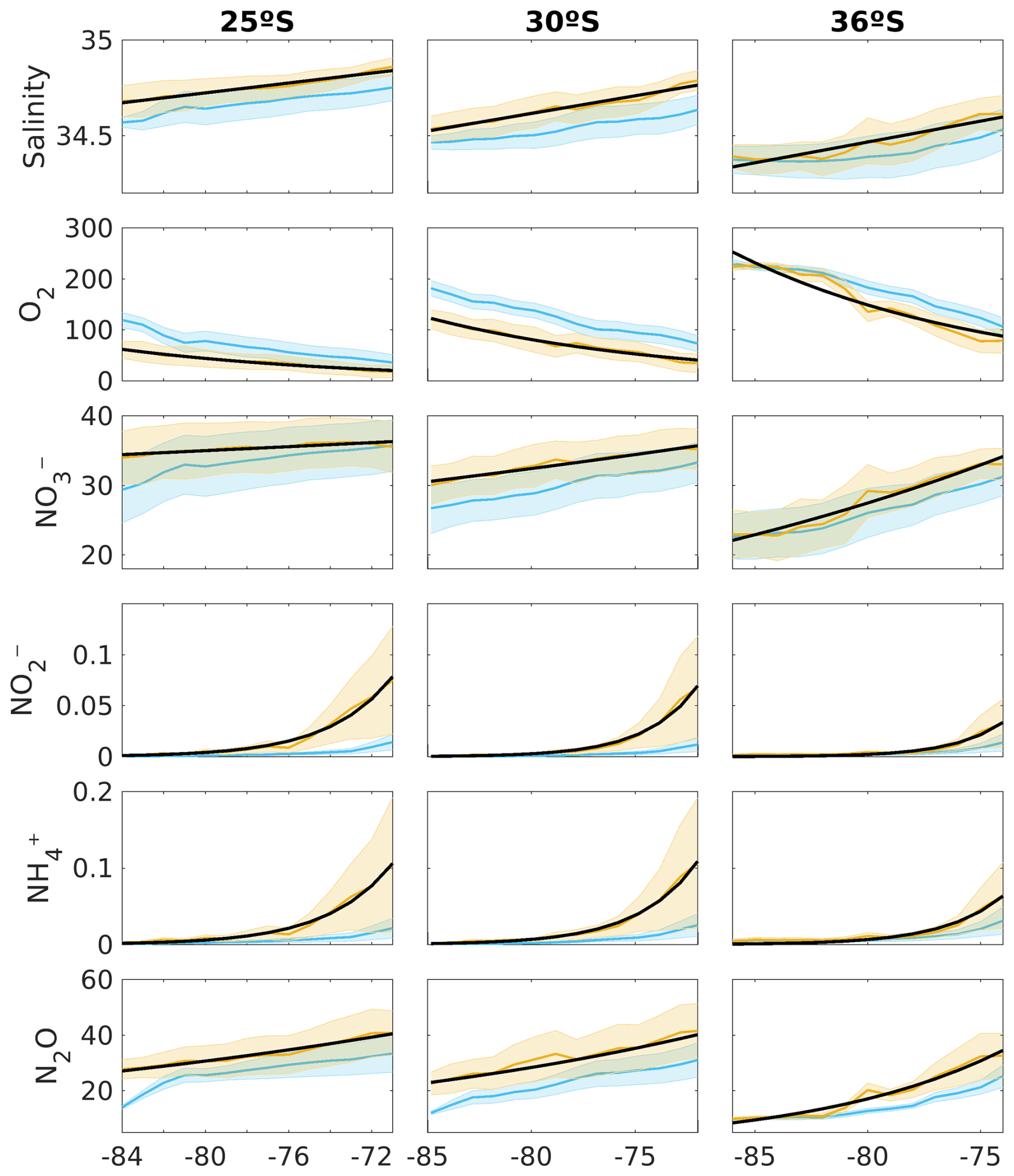
Figure 8 The orange line indicates the average biogeochemical properties of the total volume of PUDDIES identified in the zonal bands corresponding to the latitudes of 25° S (left), 30° S (middle), and 36° S (right), and the blue line indicates the mean state associated with that volume. In order from top to bottom: absolute salinity (g kg⁻¹), oxygen, nitrate, nitrite, ammonium (µM), and nitrous oxide (nM). The x axis shows the longitude in degrees west. At 25, 30, and 36° S, 862, 810, and 658 PUDDY profiles were considered, respectively. The shading indicates the standard deviation among the PUDDIES. The black line stands for the result of an exponential model of the form $y=A{e}^{-kx}$ that provides the decay rate of mean biogeochemical properties with increasing distance from the coastal zone (see Table 4 for values of k for both mean state and PUDDIES).

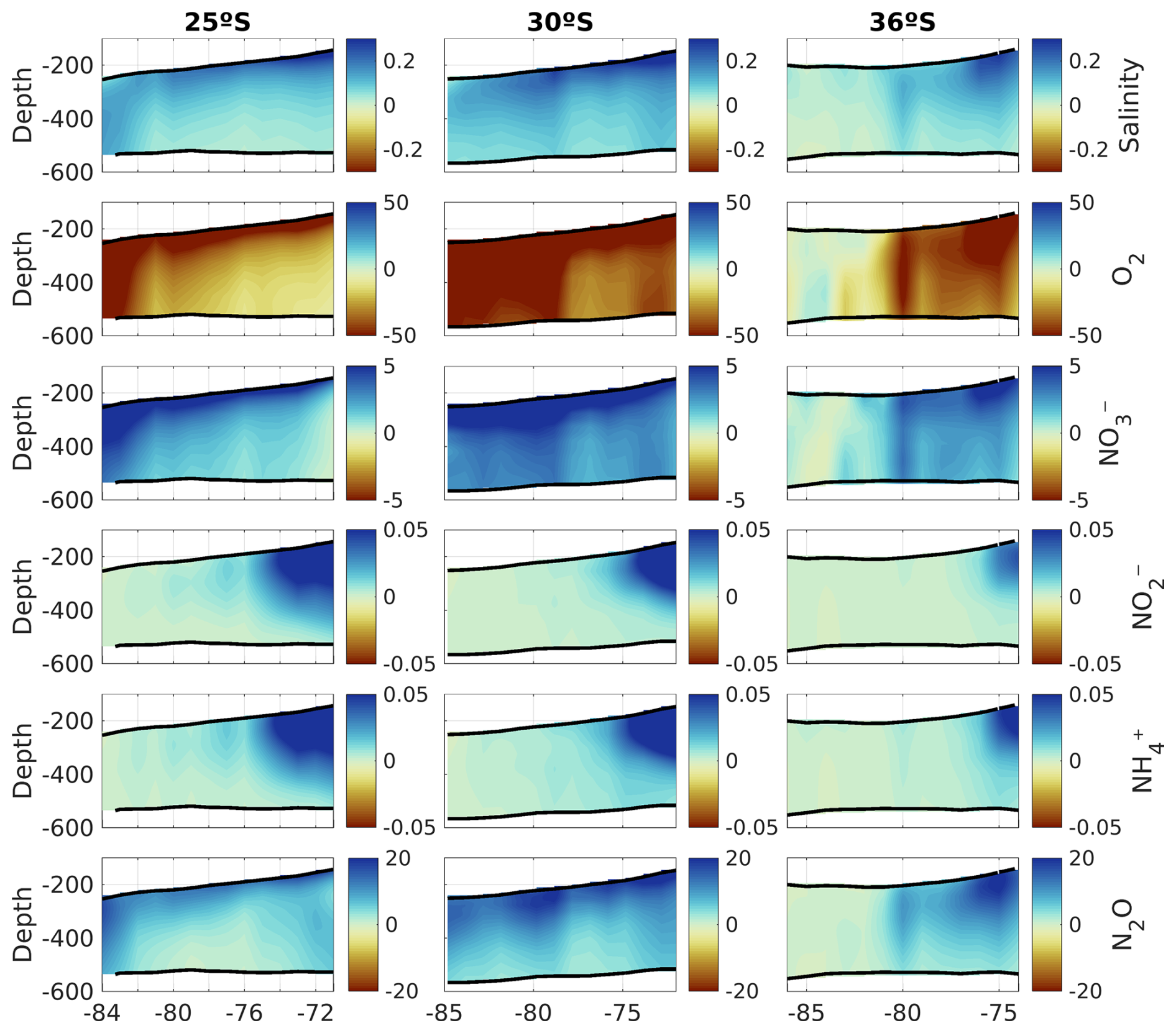
Figure 9 PUDDIES' composite anomalies for tracers along three zonal bands at different latitudes (25° S – left, 30° S – middle, and 36° S – right). In order from top to bottom: absolute salinity (g kg⁻¹), oxygen, nitrate, nitrite, ammonium (µM), and nitrous oxide (nM). Anomalies are only shown between the isopycnal layers S_upper and S_lower (black contours). The x axis shows the longitude in degrees. The number of PUDDIES used for the composites is identical to that used for Fig. 8.

We compared the characteristics acquired by PUDDIES in the subsurface band corresponding to 25, 30, and 36° S with the mean state of the same volume (Fig. 8). First, we observed a decrease in salinity farther from the coast, which indicates the intrusion of external waters distinct from the ESSW. At 25° S, PUDDIES farther from the coast retain saltier water with higher nitrate concentrations (16 % higher than the mean state) and lower oxygen levels (49 % less than the mean state) than those at 30° S (12 % increase in NO${}_{\mathrm{3}}^{-}$ and 33 % decrease in O₂) and 36° S (which becomes completely mixed). Decay rates in PUDDIES at 30° S are higher than the mean state, except for NO${}_{\mathrm{3}}^{-}$ and N₂O, while at 36° S, only N₂O exhibits a lower decay rate in PUDDIES (Table 4). At 25° S, the opposite is observed, with lower decay rates in PUDDIES except for NH${}_{\mathrm{4}}^{+}$ and NO${}_{\mathrm{3}}^{-}$. However, the biogeochemical concentrations in both PUDDIES and the mean state gradually decrease southward. PUDDIES' contributions are generally higher at 30° S, as shown by anomalies highlighting low O₂ and high NO${}_{\mathrm{3}}^{-}$ and N₂O concentrations (Fig. 9). At 25° S, PUDDIES input more NH${}_{\mathrm{4}}^{+}$ and NO${}_{\mathrm{2}}^{-}$ (∼400 % higher than the mean state) in the subsurface band near the coastal zone, while in the oceanic zone, NO${}_{\mathrm{3}}^{-}$ and N₂O (∼200 % more than the mean state) are the primary contributions, alongside waters with low O₂. The maximum contribution of NO${}_{\mathrm{2}}^{-}$ occurred at 30° S, with a 460 % increase compared to the mean state near the coastal zone. At 36° S, PUDDIES show increased contributions in the transition zones, unlike at other latitudes, with salinity, NO${}_{\mathrm{2}}^{-}$, and NO${}_{\mathrm{3}}^{-}$ maintaining high concentrations up to 76° W. N₂O also exhibits higher contributions from PUDDIES at 36° S, particularly in the near-coastal (29 % higher than the mean state) and transitional zones. NH${}_{\mathrm{4}}^{+}$ and NO${}_{\mathrm{2}}^{-}$ concentrations are highest near the formation zones at all three latitudes and decrease sharply in the transitional zones or at the beginning of the oceanic zone. In the northern regions, where the OMZ is broader and there is less differentiation between water masses, in contrast, farther south, the SAAW erodes the OMZ, making it narrower and causing more abrupt biogeochemical changes between the coastal and transition zones.

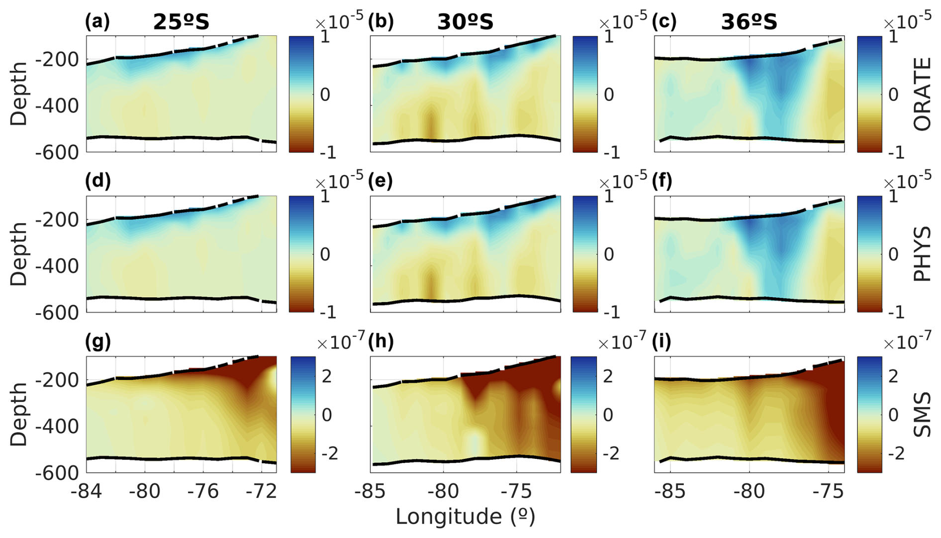
Figure 10 Same as Fig. 9 but for the main terms of the O₂ budget: (a–c) the rate of change of oxygen, (d–f) the sum of all physical processes, and (g–i) source minus sink (SMS) of biogeochemical processes.

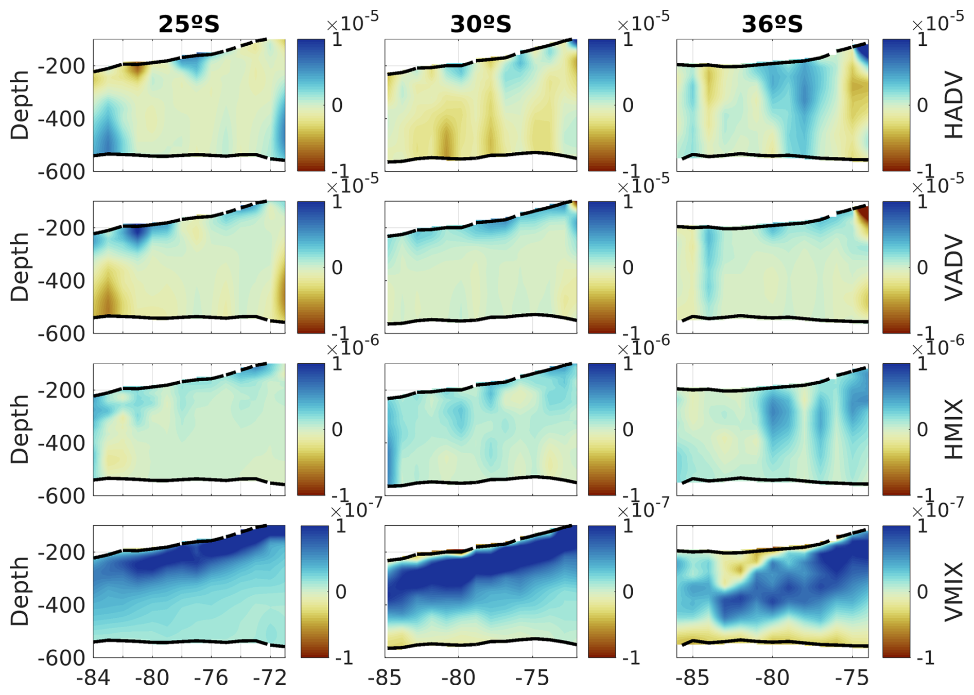
Figure 11 Same as Fig. 10 but for the various contributions of PHYS (see Eq. 1). From top to bottom: horizontal advection (HADV), vertical advection (VADV), horizontal mixing (HMIX), and vertical mixing (VMIX).

Additionally, the dynamics associated with each latitude could drive different changes. The net oxygen budget, referred to as O-RATE in Fig. 10, shows that in the upper parts of the eddies, there is always a positive oxygen contribution into the PUDDIES, with ventilation increasing in the southern eddies within the transitional zone, as seen at 36° S. Oxygen primarily enters through physical processes, with horizontal and vertical advection (HADV and VADV) being dominant (Fig. 11). Oxygen depletion in PUDDIES is also influenced by advective processes, which allow the inflow of less oxygenated waters, ventilating the cores primarily in the middle and lower parts of the eddies (30° S band) or distributed between the S_upper and S_lower layers in the near-coastal zone (36° S band). Oceanic regions (up to ∼800 km offshore) in the 30 and 36° S bands show intensified SMS activity (e.g., ammonification, zooplankton excretion, and nitrification; Figs. 10 and 11). To estimate the time PUDDIES take to cover a certain distance (i.e., 100 km (∼1°)), we could consider a propagation speed of ∼2 km d⁻¹ similar to surface eddies (Chaigneau et al., 2009; Hormazabal et al., 2013). Accordingly, it would take them approximately 50 d to travel that distance. Then, the observed SMS <0 in the oceanic zone at 30° S remained in the PUDDIES for about a year.

At 30° S and 36° S, SMS <0 extends into the lower parts of the eddies near the coastal zone more intensely (∼100–150 d), potentially prolonging the lifespan of NO${}_{\mathrm{2}}^{-}$ and NH${}_{\mathrm{4}}^{+}$. Furthermore, lower oxygen concentrations intrude through HADV and VADV, particularly at 36° S.

4 Discussion

Several studies have reported in situ subsurface eddies with similar biogeochemical characteristics to those observed in the present study (Stramma et al., 2013, 2014; Cornejo D'Ottone et al., 2016; Arévalo-Martínez et al., 2016; Grundle et al., 2017; Hormazabal et al., 2013; Karstensen et al., 2017). However, studies focused on a detailed recycling of bioelements within these eddies are scarce. While recent studies have used high-resolution coupled models to describe and quantify more complex processes involved in the O₂, nutrient, or organic matter balance within eddies (José et al., 2017; Frenger et al., 2018; Lovecchio et al., 2022), the agents generating natural variability in the lifespan of these bioelements associated with the nitrogen cycle during their trajectory from the OMZ to oceanic waters have not been analyzed in detail.

In this work, a robust statistical analysis was conducted considering all PUDDIES identified over a 9-year period using two approaches. In the first approach, we characterized the biogeochemical signal of the source water inside the PUDDIES. Subsequently, we analyzed the eddy cores, focusing on the average PUDDY profiles (using δh_max; see Sect. 2.6.1) and presented the values in the isopycnal layer of 26.6 kg m⁻³ to assess how and to what extent the biogeochemical properties of the PUDDY cores differ across various regions of the SEP from their formation zone (results in Sect. 3.1, 3.2, and 3.3).

In the second approach, we considered the entire volume of the PUDDIES to characterize their average conditions and quantify how these properties modify the intrathermocline band where the PUDDIES travel – from the coastal zone, through the transition zone, and into the oceanic zone (see Sect. 3.4). Additionally, we evaluated the balance of processes involved in the interaction of the PUDDIES along their trajectory (details in Sect. 3.3 and 3.4). This analysis allowed us to identify differences in the impact of PUDDIES at different latitudes and gain a deeper understanding of the processes involved.

4.1 Biogeochemical anomalies in PUDDIES from their formation

Subsurface anticyclonic eddies appear to be formed by separating the Peru–Chile Undercurrent from the slope (e.g., Molemaker et al., 2015; Thomsen et al., 2016; Contreras et al., 2019). Here, we observed a higher recurrence of PUDDIES in specific sectors, namely, between 29 and 35° S (Fig. 1b), related to the widening of the continental shelf. This change in topography may lead to greater separation of the PCUC from the slope, creating favorable conditions for the generation of PUDDIES, as observed by Chaigneau et al. (2009). PUDDIES appear to originate from instabilities forced in the bottom boundary layer at the upper continental slope, where the core of the PCUC interacts with the sea bottom (Contreras et al., 2019) and where the core of the OMZ is observed. This water, trapped within the PUDDIES, is characterized by positive NH${}_{\mathrm{4}}^{+}$, NO${}_{\mathrm{3}}^{-}$, NO${}_{\mathrm{2}}^{-}$, and N₂O anomalies and very low O₂ that vary with latitude, as described in Sect. 3.1. However, unlike O₂ and salinity, which exhibit a more uniform gradient along the coast, several other biogeochemical components have more irregular spatial distributions depending on whether conditions are hypoxic or suboxic.

In the northern part of the coastal zone, limited ventilation creates an environment with suboxic conditions and denitrification, resulting in NO${}_{\mathrm{3}}^{-}$ and N₂O deficits and NO${}_{\mathrm{2}}^{-}$ and NH${}_{\mathrm{4}}^{+}$ enrichment. In contrast, the central coastal waters exhibit increased NO${}_{\mathrm{3}}^{-}$, with the southern part showing higher N₂O concentrations. Additionally, as the formation of PUDDIES is associated with cross-shore velocities – exchanging nutrients between the continental shelf and open sea (Thomsen et al., 2016) – the mixture of ESSW and SAAW waters, also affected by the southward reduction in the contribution of ESSW (Fig. 2; Silva et al., 2009), enhances the biogeochemical variability of the PUDDIES generated along the Chilean coast (Fig. 3).

In summary, PUDDIES formed along the Chilean coast capture distinct biogeochemical “signatures” depending on where they form. In the north, minimal ventilation fosters suboxic conditions and denitrification, leading to deficits of NO${}_{\mathrm{3}}^{-}$ and N₂O but high NO${}_{\mathrm{2}}^{-}$ and NH${}_{\mathrm{4}}^{+}$, whereas central and southern subregions show increased NO${}_{\mathrm{3}}^{-}$ and higher N₂O. Moreover, cross-shore exchange between ESSW and SAAW further amplifies this variability, giving rise to eddies with diverse nutrient and oxygen properties as they move offshore.

4.2 Persistence of biogeochemical anomalies away from the coast

In each subregion (Fig. 1a), the PUDDIES exhibited distinct biogeochemical configurations, as summarized in Figs. 4, 5, and 6 (results in Sect. 3.2). The dominance of SAAW in the southern regions explains the largest number of hypoxic PUDDIES containing higher O₂ concentrations and lower levels of NO${}_{\mathrm{3}}^{-}$, NH${}_{\mathrm{4}}^{+}$, NO${}_{\mathrm{2}}^{-}$, and N₂O compared to PUDDIES farther north, where suboxic cores are more prevalent (Silva et al., 2009). Consequently, PUDDIES that capture a larger fraction of ESSW during their formation exhibit biogeochemical contributions closer to the P75 (Fig. 5; Table S2) and show a higher O₂ deficit than the mean state. This suggests that the southern regions are experiencing greater deoxygenation and nutrient enrichment due to the influence of PUDDIES compared to the northern regions, where the OMZ is much broader.

When estimating the percentage of core distributions exhibiting hypoxia and suboxia, the results showed that hypoxic cores predominantly occur in oceanic waters (Table 2). In general, as we move away from the Chilean coast, biogeochemical element concentrations decrease significantly, though the magnitude of the decrease varies by element (Fig. 4). Although PUDDIES share common characteristics within each region, some variability is observed. This reflects the variety of drivers – such as kinetic and potential energy, vorticity, and other dynamics – as well as the differences in the properties of the source water they enclose, their trajectory (potentially interacting with different external water masses), and the physical and biogeochemical processes occurring within them during their lifespan. These factors can enhance or diminish the PUDDY's ability to transport properties far from its formation zone.

However, the results indicate an effective transport of these properties to oceanic regions, where values exceed the P90. In contrast, for the transition zones (NTZ and STZ), only AOU, salinity, and NH${}_{\mathrm{4}}^{+}$ exceed the P90, while ΔN₂O and ΔNO${}_{\mathrm{3}}^{-}$ are closer to the P75. This regional difference clearly demonstrates that the perturbations to the mean state caused by PUDDIES are more significant in the open ocean than near the coast (Figs. 4 and 5; Table S1).

4.3 Changes in the biogeochemistry of subsurface water masses by the PUDDIES

Our results showed changes from the coastal to oceanic zones across three latitudes, where a decrease in dissolved inorganic nitrogen compounds, along with a salinity decay rate, confirmed that PUDDIES age and mix with external waters as they move into the oceanic zone (Fig. 8; Table 4). Similar patterns were observed by José et al. (2017) in the upwelling system off Peru, Frenger et al. (2018) across the main EBUS, and Lovecchio et al. (2022) in the Northern Canary upwelling system. This offshore change suggests that PUDDIES have relatively permeable boundaries, but the level of coherence and isolation within the PUDDY core can significantly influence the lifespan of compounds enclosed in it. The macronutrient behavior observed was consistent with Frenger et al. (2018), though in our case, N₂O – despite its minimal concentrations – exhibited a pattern similar to other macronutrients, such as NO${}_{\mathrm{3}}^{-}$ (Fig. 8). Decay rates for NO${}_{\mathrm{2}}^{-}$ and NH${}_{\mathrm{4}}^{+}$ were faster than those for NO${}_{\mathrm{3}}^{-}$ and N₂O (Table 4).

Nitrate showed higher concentrations compared to other nitrogen compounds. Additionally, as long as NH${}_{\mathrm{4}}^{+}$ and NO${}_{\mathrm{2}}^{-}$ are present (Figs. 4, 8, and 9), nitrification can replenish the NO${}_{\mathrm{3}}^{-}$ pool in subsurface waters where photosynthesis does not consume it. In addition, N₂O production depends on [NH${}_{\mathrm{4}}^{+}$], [NO${}_{\mathrm{2}}^{-}$], and [O₂] levels and the nitrification and denitrification processes. According to the model parameterization (for more details, see Gutknecht et al., 2013), the maximum N₂O production occurs when O₂=1 µM, with SMS(N₂O) =α(Nitrif) +β(Nitrif) (α, β constant), whereas when O₂ is high or O₂<1 µM, the N₂O production decreased because SMS(N₂O) → α(Nitrif). On one hand, N₂O production diminishes as NO${}_{\mathrm{2}}^{-}$ and NH${}_{\mathrm{4}}^{+}$ availability declines, as observed in the open sea; on the other hand, in coastal zones, denitrification rapidly depletes these compounds until N₂O production ceases at oxygen concentrations below 1 µM. Since the model does not account for N₂O consumption by biological processes (via denitrification or fixation) but only through atmospheric exchange, the PUDDIES act as a source of N₂O as they move offshore and the observed N₂O decrease within PUDDIES can only result from physical processes facilitating exchange with external waters.

Notably, the 30° S zonal band exhibited the largest anomalies in biogeochemical characteristics (Fig. 9). Along this band, the high occurrence of PUDDIES, including those formed at or south of this latitude, is significant due to the characteristic northwest trajectory of eddies. This could explain the high nutrient concentrations there (Fig. 3). Newly formed PUDDIES must be supported by dissolved organic nitrogen from the source water with higher O₂ consumption (SMS) during the first 100–150 d, as Lovecchio et al. (2022) proposed. Mixing with external waters (Fig. 8) is driven by physical processes, particularly advection (HADV and VADV, Figs. 10 and 11). Compared to the other two latitudes, higher O₂ consumption (SMS <0) at 30° S suggests higher local nutrient production through remineralization (i.e., more organic material is being broken down), potentially extending the lifespan of NO${}_{\mathrm{2}}^{-}$ and NH4⁺, which are necessary for the ΔN₂O and ΔNO${}_{\mathrm{3}}^{-}$ activity that remained in the PUDDIES for about a year around 800 km offshore. Biological activity sustains low-oxygen cores for longer periods, preserving original conditions even with O₂<20 µM in the cores, where denitrification continues while the edges ventilate. Additionally, horizontal advective processes further reduce oxygen levels in the lower part of the eddy by allowing the intrusion of low-oxygen waters, contrasting with observations at 25 and 36° S.

This combination of conditions suggests that regions of significant interaction with PUDDIES can transform the biogeochemistry of the subsurface layer in meaningful ways. Both approaches used to characterize PUDDIES provide valuable insights into how and to what extent these PUDDIES evolve, driving changes in the intrathermocline from their formation to their dispersion across the SEP.

4.4 Advantages and disadvantages of the model for low-oxygen conditions

We now discuss the limitations of the model formulation in accounting for the transition between the two oxygen regimes (hypoxic versus suboxic) and its implications for PUDDIES' life cycle. AOU : NO${}_{\mathrm{3}}^{-}$ ratios of 250:30 (up to 20:1) have been documented in the Atlantic from in situ monitoring of NO${}_{\mathrm{3}}^{-}$ within mode water eddies (Karstensen et al., 2017) and in eddy cores with NO${}_{\mathrm{3}}^{-}<\mathrm{25}$ µM at O₂<5 µM in the SEP (Stramma et al., 2013). The eddies modeled here showed AOU values similar to those found by Karstensen et al. (2017) in the eastern tropical North Atlantic, although NO${}_{\mathrm{3}}^{-}$ was overestimated by 3–5 µM, leading to an AOU : ΔNO${}_{\mathrm{3}}^{-}$ ratio of 5:1 (Figs. 4b and 6 – upper box; Stramma et al., 2013). Suboxic PUDDIES build up NO${}_{\mathrm{2}}^{-}$, although the modeled maximum concentration appears underestimated compared to previously reported in situ data (Stramma et al., 2013; Cornejo and Farías, 2012; Cornejo D'Ottone et al., 2016). Consequently, the relationship between NO${}_{\mathrm{2}}^{-}$ and ΔN₂O in the northern zone also showed an underestimation. At the modeled N₂O maximum (>30 nM, Fig. 6), field data show NO${}_{\mathrm{2}}^{-}$ values >1 µM (Cornejo and Farías, 2012), while the modeled NO${}_{\mathrm{2}}^{-}$ maximum reaches 0.15 µM (Figs. 4 and 5). Comparing our results with eddies monitored in the SEP, the N₂O concentrations observed in open ocean eddies agree with those measured by Cornejo D'Otonne et al. (2016; Figs. 4d, S5) in an eddy originating near the coast off Concepción (∼37° S, south zone), although there are differences of up to 20 nM with the eddy reported by Arévalo-Martínez et al. (2016; Figs. 4d, S5) off northern Chile. These results suggest a better representation of biogeochemical processes by the model in a hypoxic rather than suboxic environment.

Biogeochemical components are challenging to model due to the numerous physical, biogeochemical, and biological processes involved. Specifically, under hypoxic or suboxic conditions, the nitrogen cycle is more complex due to additional processes that occur within a narrow O₂ range, increasing the system's sensitivity. Processes removing nitrogen from the system, such as denitrification, also generate intermediate products, such as N₂O and NO${}_{\mathrm{2}}^{-}$ (e.g., denitrification, NO${}_{\mathrm{3}}^{-}$ reduction). Denitrification is a complex process to parameterize, involving a range of steps for each nitrogen component and various rates of decomposition of particulate (large and small) and dissolved material. However, despite the attempt to consider these processes realistically, the model remains an approximation but reasonably represents the involved processes, primarily within the intrathermocline band (see Appendix A). In the suboxic zone, while the model underestimated O₂, NO${}_{\mathrm{3}}^{-}$ remained overestimated, but in the subsurface band associated with the OMZ core, the model represented the lowest biases in O₂ and nitrogen evaluated with climatological observations (see Appendix A). This allowed us to present a robust statistical analysis of biogeochemical properties inside and outside the PUDDIES. Despite the difficulty in simulating realistically sharp mean gradients in water mass properties (Pizarro-Koch et al., 2019), the model did highlight typical features, such as NO${}_{\mathrm{3}}^{-}$ consumption and production of NO${}_{\mathrm{2}}^{-}$ and N₂O, and processes that persist within PUDDIES far from their origin within the OMZ.

5 Conclusions

Using a high-resolution coupled simulation of the SEP, we characterized the biogeochemical changes within PUDDIES, their differences with the external properties, and the processes involved in the O₂ balance during their transport to oceanic waters. The model resolved eddy dynamics and biogeochemical processes related to the nitrogen cycle, including characteristic EBUS processes such as denitrification. This methodology allowed us to statistically approximate the biogeochemical changes occurring within these PUDDIES, quantify the modifications to water bodies along their paths, and identify the dominant mechanisms regulating compound concentrations from the formation zone to hundreds of kilometers offshore.

During formation, PUDDIES capture a biogeochemical signal that varies depending on their origin, which is associated with the core of the Peru–Chile Undercurrent. Peripheral permeability enables exchange with external waters, modulating the original signature. However, the core signal retains characteristic negative O₂ anomalies and positive anomalies for other biogeochemical tracers. These disturbances may cause average properties to exceed the 90th percentile (P90) in the open ocean, in contrast to the formation zone, where values remain above the 50th percentile (P50). While a high percentage of PUDDIES near the coast exhibit suboxic cores (all in the north and 70 % in central-south Chile), the proportion decreases with distance from the coast, where hypoxic cores become predominant (60 % in the STZ and NOZ). This suggests core ventilation during their trajectory, as indicated by an estimate of the salinity decay rate as a function of latitude.

The dominant mechanism for O₂ exchange in the eddy core is lateral and vertical advection, with vertical mixing contributing 2 orders of magnitude less. O₂ consumption through biological activity (SMS) was maintained inside the PUDDIES (around 6 to 12 months) up to the oceanic zones (e.g., at 30° S, the O₂ consumption was maintained up to ∼800 km from the coast), enabling the persistence of low O₂ conditions in the core despite peripheral ventilation. This persistence supports processes such as denitrification, which occur under hypoxic or suboxic conditions within the OMZ and can extend into areas far beyond the OMZ, sustained in core niches with O₂<20 µM. The SCZ and STZ experience significant deoxygenation and nutrient enrichment due to PUDDIES formed with larger anomalies. At 30° S, a combination of factors significantly impacts the intrathermocline biogeochemistry due to PUDDIES transiting this latitude. The maximum contribution of NO${}_{\mathrm{2}}^{-}$ occurred at 30° S, with a 460 % increase compared to the mean state, near the coastal zone. Clearly, the formation of PUDDIES is a critical process in extending the OMZ boundaries at its southern edge. Additionally, the interplay of physical conditions can generate regions with substantial subsurface water mass changes due to interactions with PUDDIES.

Biogeochemical tracers exhibit varying lifespans depending on their original concentrations, as well as their demand and production rates. Ammonium (NH${}_{\mathrm{4}}^{+}$) and nitrite (NO${}_{\mathrm{2}}^{-}$) tend to decline first, with their concentrations being highest in the coastal zone (300 %–400 % higher than the mean state) and exhibiting high decay rates with distance from the coast, while other components decrease more slowly and persist longer. Despite being produced in low concentrations, N₂O is retained in PUDDIES farther from the coast, serving as a proxy for denitrification in the source water and contributing to the subsurface reservoir of this greenhouse gas in the open ocean (up to ∼100 % higher than the mean state). Characterizing PUDDIES provides valuable insights into how they evolve and drive intrathermocline changes from their formation to dispersion across the SEP. Beyond offering insights into the biogeochemical dynamics of PUDDIES, this study's findings can also help guide in situ monitoring, particularly in remote areas where unusual biogeochemical signals may indicate the presence of a PUDDY.

Higher-resolution models enable better characterization of mixing processes involved in eddy core ventilation and the exchange of properties with external waters through submesoscale dynamics (Brannigan et al., 2017). Coupling with more complex biogeochemical models will help quantify the effects of additional SMS processes within PUDDIES not included in this study. This is planned for future research. Validation and supplementary statistics through further observations in the study area are also recommended to deepen our understanding of coupled processes in surface and subsurface eddies.

Appendix A: Model assessment

A1 Data

Observed climatological O₂ and NO${}_{\mathrm{3}}^{-}$ fields were taken from the CSIRO Atlas of Regional Seas (CARS2009; https://doi.org/10.5281/zenodo.16875985, Dunn and Ridgway, 2002; Ridgway et al., 2002; Ridgway et al., 2025) for the biogeochemical model assessment, which has a spatial resolution of 0.5° and a monthly mean resolution. The model validation was performed over the first 800 m. The vertical resolution of the data set is 10 m to the first 300 m, 25 to 500 m, and 50 m down to 800 m.

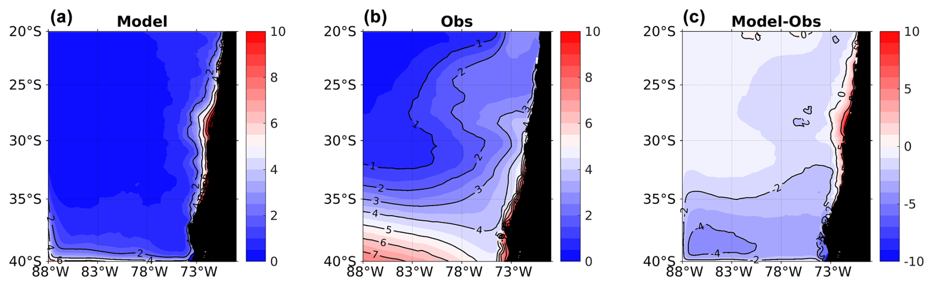
Figure A1 Spatial distribution of mean surface NO${}_{\mathrm{3}}^{-}$. (a) ROMS-BioEBUS simulation, (b) CARS climatology, and (c) BIAS (model–observations). Units are µM.

A2 Surface nitrate

The model simulates low NO${}_{\mathrm{3}}^{-}$ (<2 µM) in general, except in the areas near the coast and in the southwest, where concentrations reached 8 µM (Fig. A1a). The observed concentrations were higher, particularly in the south (Fig. A1b). Overall, the model underestimated NO${}_{\mathrm{3}}^{-}$ concentrations in most of the domain, although the differences with observations remain relatively small, ranging between 0 and 4 µM south of 30° S and between 0 and 2 µM north of 30° S (Fig. A1a, c). Adjacent to the coast between 25 and 35° S, the model overestimates concentrations by ∼7 µM (Fig. A1c). In general, differences were minimal over most of the study area, and it can therefore be considered that the model represents surface NO${}_{\mathrm{3}}^{-}$ fairly well.

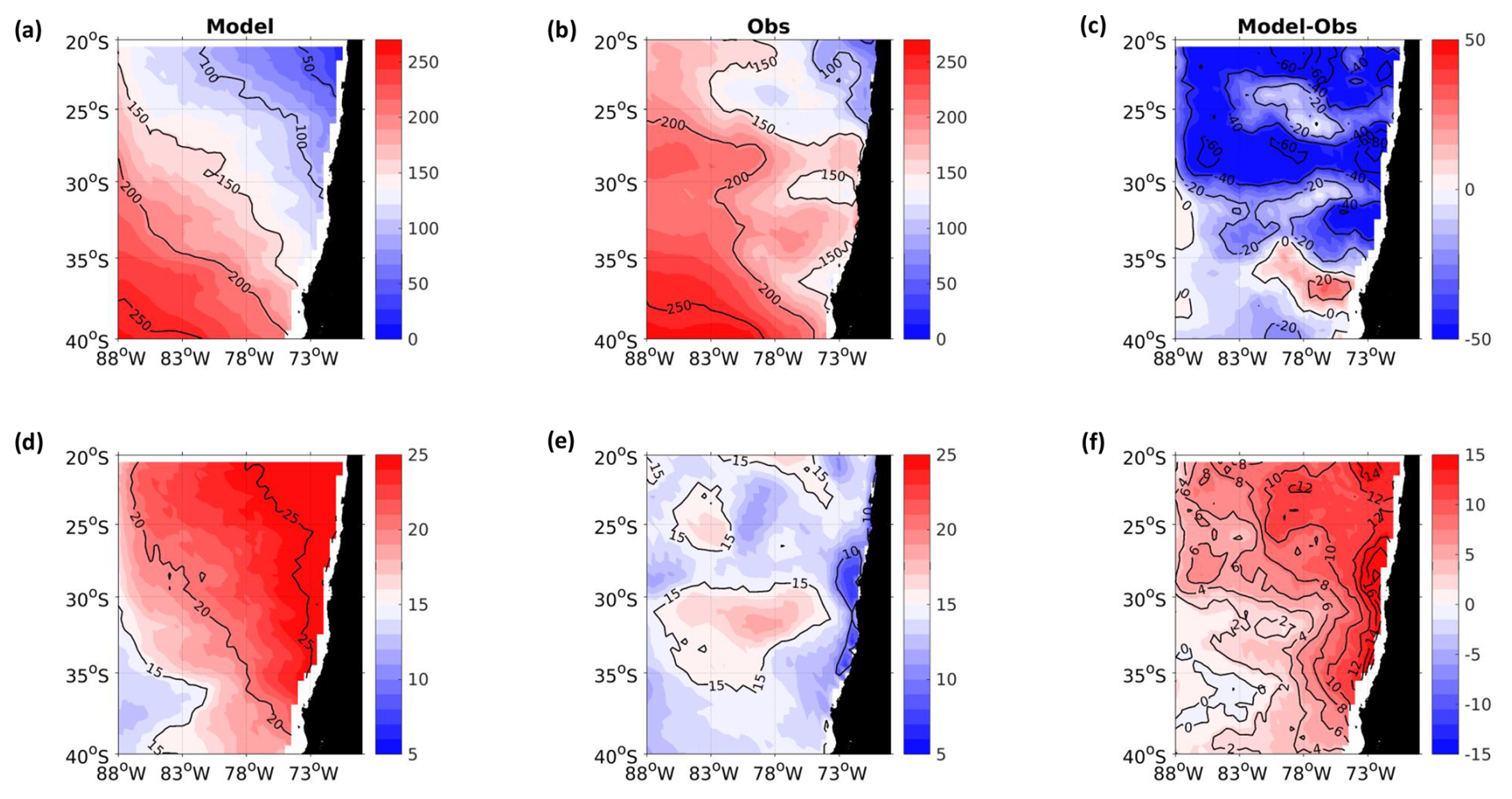
Figure A2 (a–c) Mean O₂ and (d–f) mean NO${}_{\mathrm{3}}^{-}$ concentration in the isopycnal layer S_upper=26.0 kg m⁻³ from the ROMS-BioEBUS simulation (a, d), the CARS climatology (b, e), and the BIAS (c, f). Units are µM.

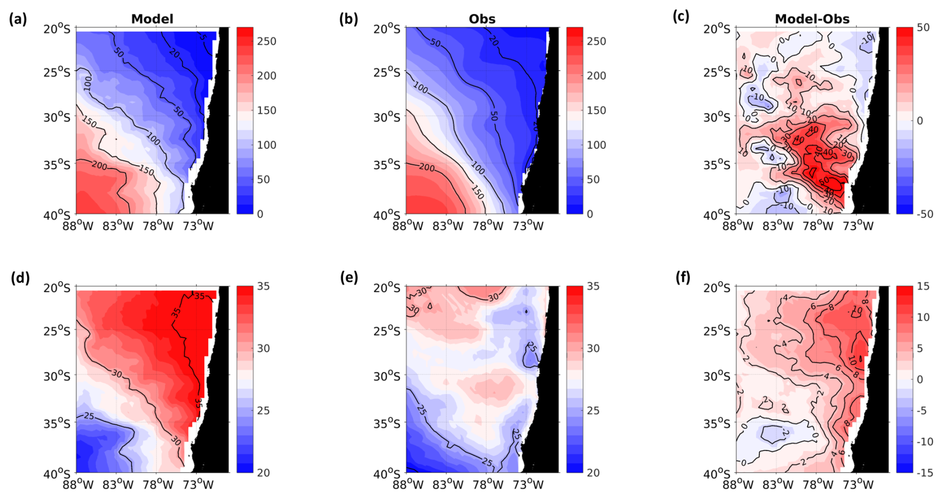
Figure A3 Same as Fig. A2 but for the isopycnal layer S_core=26.6 kg m⁻³.

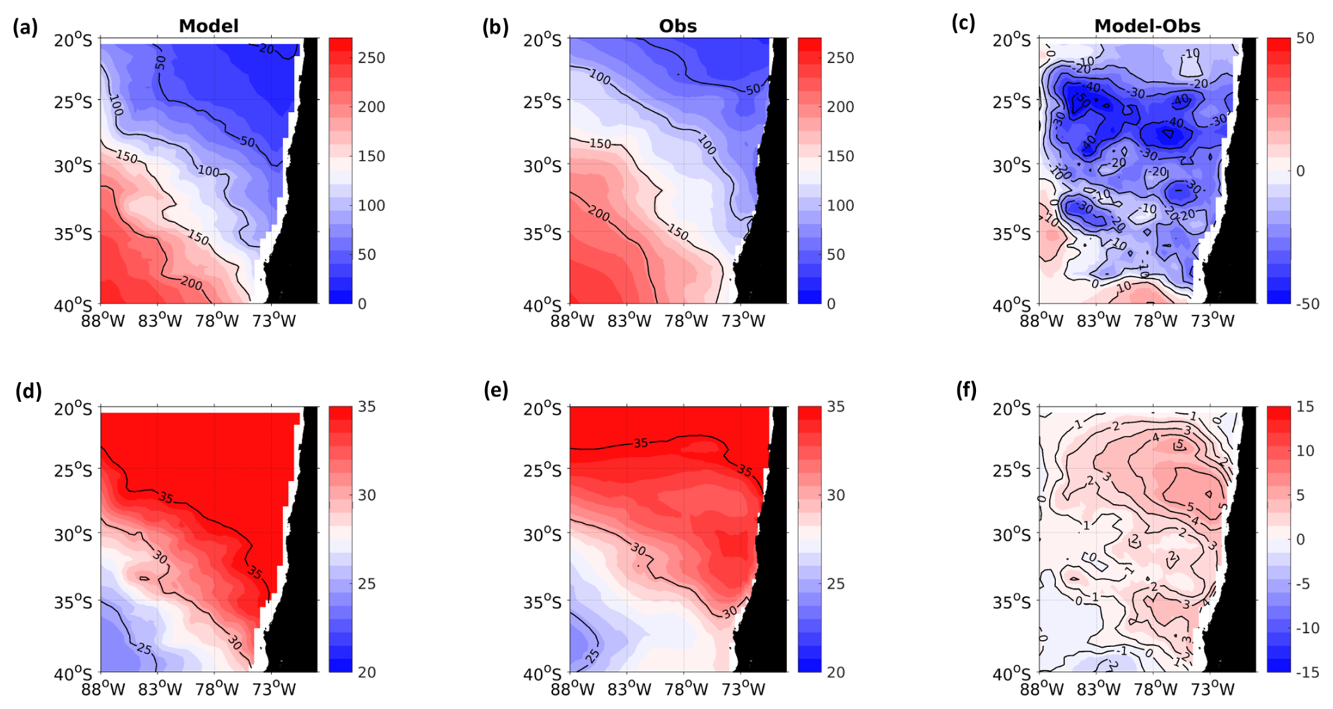
Figure A4 Same as Fig. A2 but for the isopycnal layer S_lower=26.9 kg m⁻³.

A3 Oxygen and nitrate on the isopycnal layers

The comparison between observations and the model is carried out over different density layers S_upper, S_lower, and S_core (Figs. A2, A3, A4). The model captures the principal characteristics of O₂ and NO${}_{\mathrm{3}}^{-}$, displaying a similar structure and latitudinal and zonal gradients. Compared with observed data, lower O₂ concentrations and higher NO${}_{\mathrm{3}}^{-}$ concentrations were predicted near the coast and north of 30° S associated with the meridional changes of the offshore extension of the OMZ.

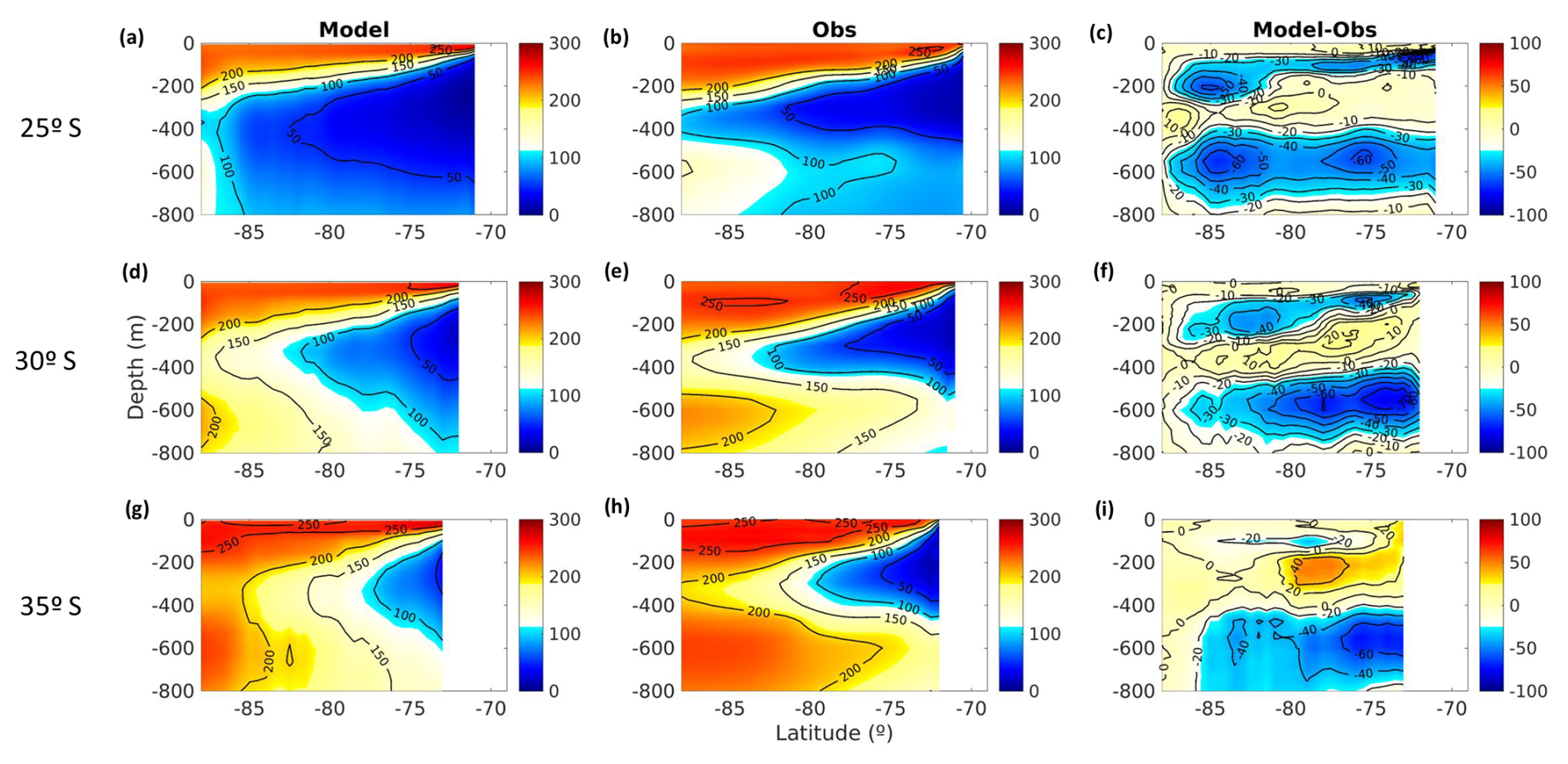
Figure A5 Zonal section of mean O₂ concentration at (a–c) 25° S, (d–e) 30° S, and (f–h) 35° S (a, d, g) from the ROMS-BioEBUS simulation (left boxes), CARS climatology (middle boxes), and BIAS (right boxes). Units are µM.

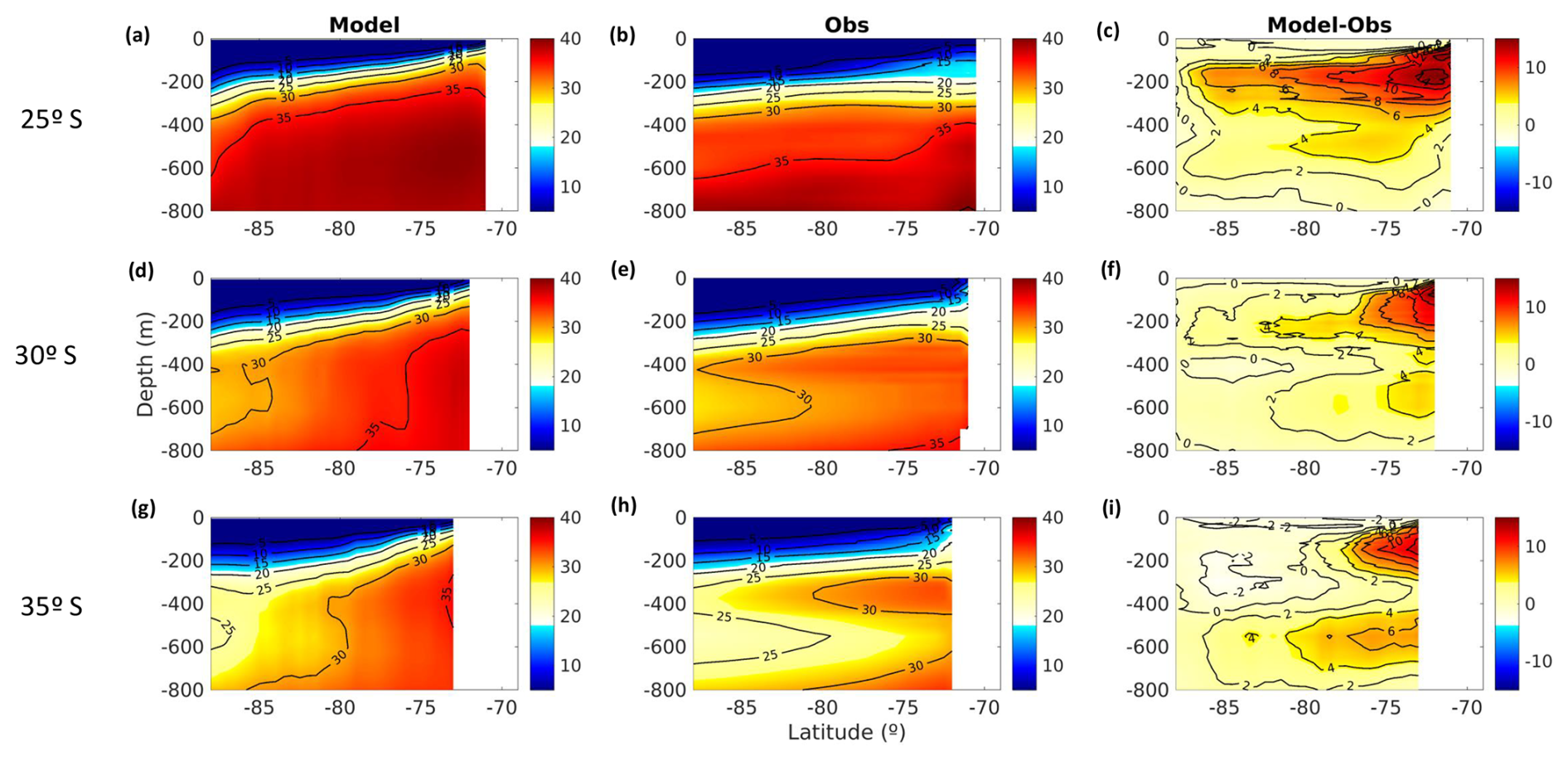
Figure A6 Same as Fig. A5 but for mean NO${}_{\mathrm{3}}^{-}$ concentration.

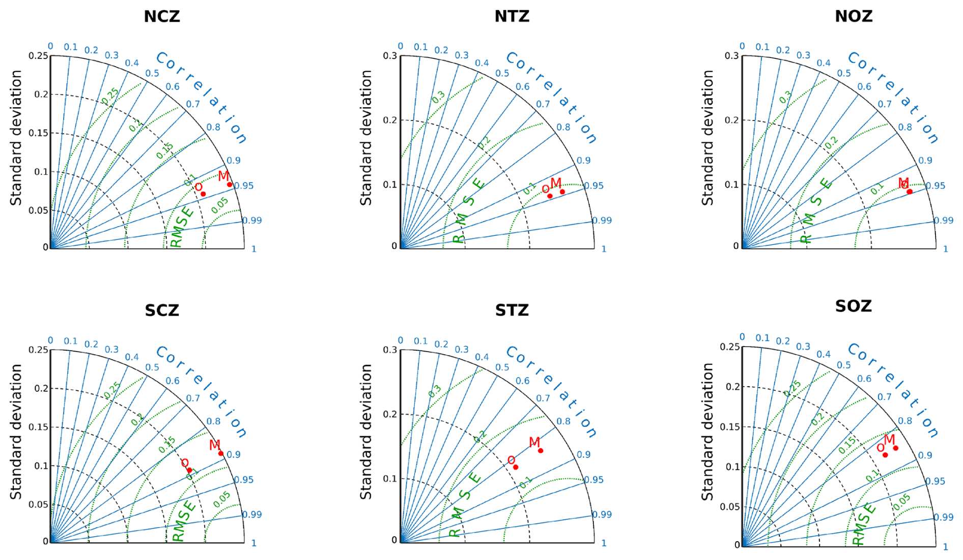
Figure A7 Taylor diagram for mean O₂ concentrations over the six subregions (Fig. 1a) and within the first 800 m. M is for the model, while O is for the CARS climatology. The x-y axis refers to the standard deviation (black lines), correlations are shown in the radial axis (blue lines), and RMSE is indicated by curved lines (green). Region names are: Northern Coastal Zone (NCZ), Northern Transition Zone (NTZ), Northern Oceanic Zone (NOZ), Southern Oceanic Zone (SOZ), Southern Transition Zone (STZ), and Southern Coastal Zone (SCZ).

Figure A8 Same as Fig. A7 but for mean NO${}_{\mathrm{3}}^{-}$ concentration.

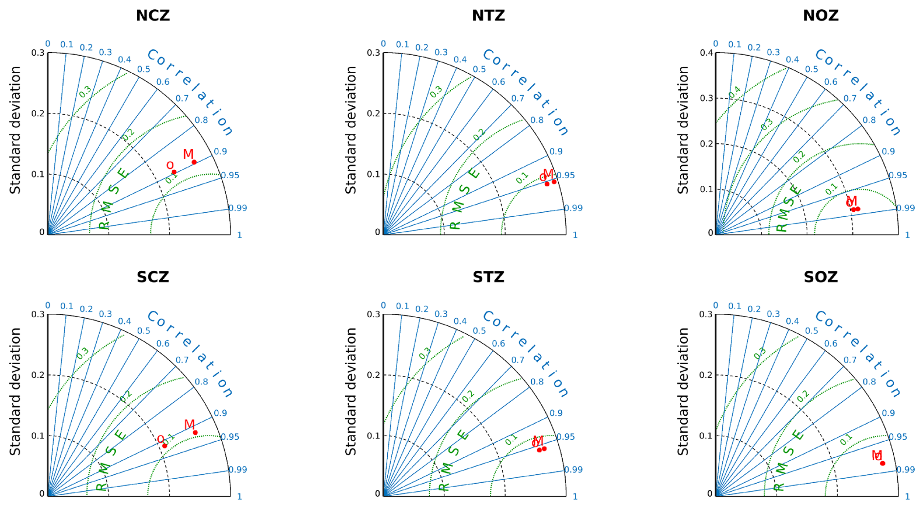
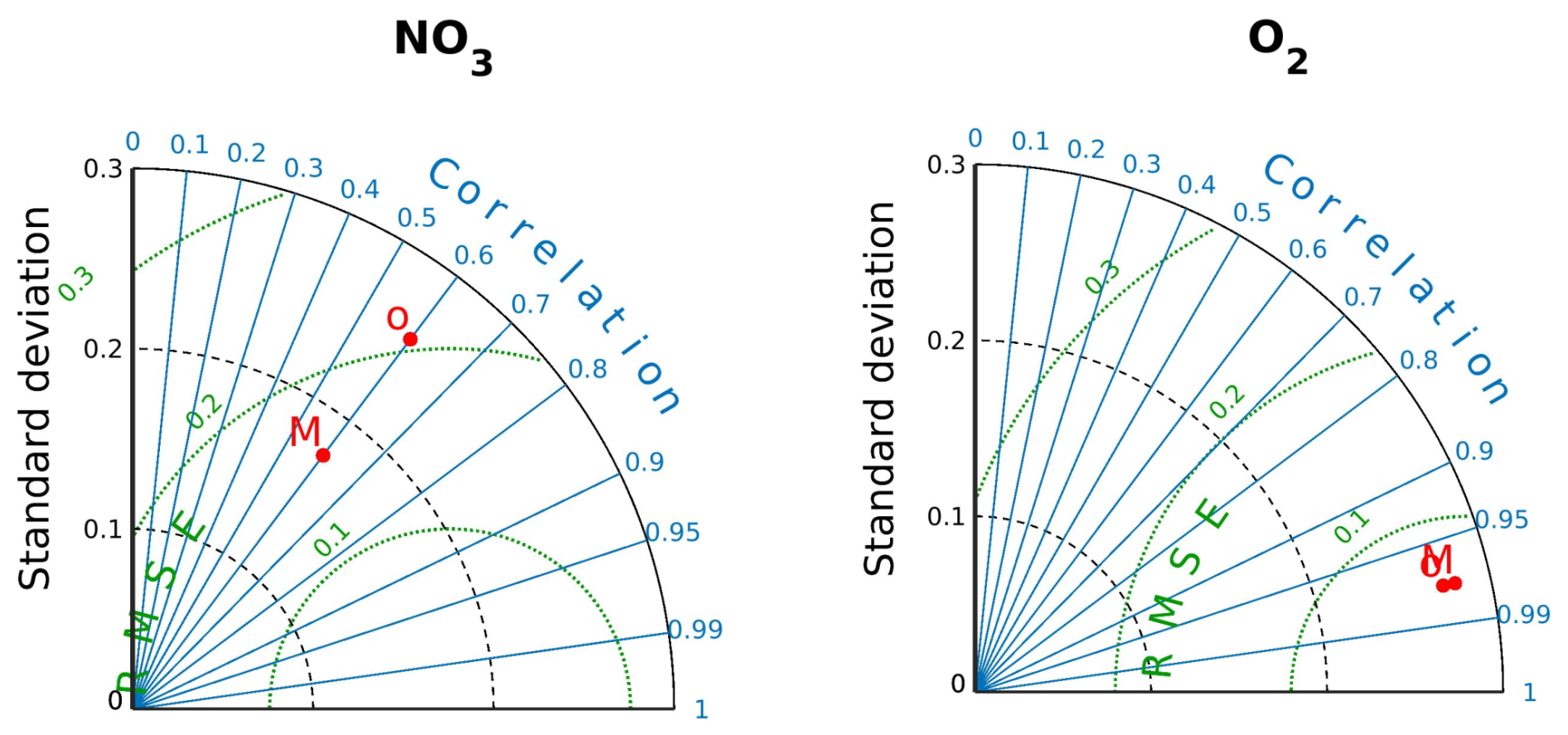
Figure A9 Taylor diagram for mean NO${}_{\mathrm{3}}^{-}$ and O₂ concentrations over the entire S_core volume. Details are similar to those in Figs. A7 and A8.

In the S_upper surface, observations reveal discontinuous areas with lower O₂ concentrations north of 25° S (O₂<100 µM), between 30–31 and 35–36° S (O₂<150 µM). The model mostly underestimated these O₂ concentrations by 40 µM north of 30° S and by around 20 µM between 30 and 35° S and overestimated them by 20 µM between 35 and 38° S near the slope but performed better south of 35° S offshore. For NO${}_{\mathrm{3}}^{-}$, observations indicated very low concentrations mainly along the coast between 23 and 35° S (<10 µM), with an increase to >15 µM in the oceanic region. Therefore, the model overestimated concentrations in the coastal zone (>10 µM) and in the northern oceanic zone (4–8 µM, Fig. A2).

Regarding the S_core layer, the model performed better in the northern region, underestimating O₂ concentrations between 0 and 10 µM. Off the coast, the bias ranged from −10 to 10 µM. However, south of 30° S, between 75 and 80° W, the model overestimated O₂ concentrations by over 40 µM, whereas west of 82° W, the bias varied between −10 and 10 µM. Nitrate concentration is overestimated by the model in the coastal region with concentrations exceeding 6–8 µM, particularly in the northern oceanic area (2–4 µM). The model is more realistic in terms of NO${}_{\mathrm{3}}^{-}$ in the region west of 78° W and south of 30° S (Fig. A3).

In the S_lower layer, the model simulates generally lower O₂ concentrations than observations north of 30° S, underestimating by 10–40 µM. This bias is smaller south of 30° S (10–30 µM) and in the southwest (0–10 µM). The model realistically simulates NO${}_{\mathrm{3}}^{-}$, with deviations from observations ranging from −2 to 5 µM and with the greatest overestimation occurring in the region where O₂<50 µM (Fig. A4).

A4 Vertical structure

The comparison between the model and observations is done along zonal sections at 25, 30, and 35° S (Figs. A5, A6). Along the latitudinal gradient, the contour of 50 µM shows that the OMZ narrows toward the south. Observations provide evidence of an elongated low-oxygen tongue in subsurface waters that is more pronounced than in the model simulations, along with an intrusion of oxygenated waters both at the surface and at depth (∼600 m), enclosing the low-oxygen water with a marked oxycline (Fig. A5). The oxyclines showed a greater bias, with the model tending to underestimate the observed data, particularly in the lower oxycline with an underestimation of up to 60 µM. In the subsurface layer between 200 and 400 m, the model better represents O₂ levels, especially at 25–30° S where differences ranged from 0 to 10 µM (Fig. A5c, f). At 35° S, there is an overestimation (40 µM) between 75 and 80° W at a low depth of 200–300 m (Fig. A5i).

Along 25° S, the model simulates higher subsurface NO${}_{\mathrm{3}}^{-}$ concentrations near the coast compared to observations, showing differences of up to 15 µM. Below 400 m of depth, overestimations range from 0 to 4 µM (Fig. A6a, b, c). These differences decrease toward the south; at 30 and 35° S, the most significant differences extend from the coast to 76° W and below −300 m (overestimations of 8–12 µM), whereas elsewhere, the differences remain between 0 and 4 µM. Subsurface NO${}_{\mathrm{3}}^{-}$ is underestimated by 2 µM by the model at 35° W and west of 80° W (Fig. A6f, i).

Taylor diagrams synthesize the agreement between model and observations for the annual mean O₂ and NO${}_{\mathrm{3}}^{-}$ in each of the subregions integrated in the upper 800 m of the water column (Figs. A7, A8). Estimates of standard deviation, correlation, and RMSE reveal that the current model configuration is generally in reasonable agreement with observations, primarily in the subsurface layer where most of the properties of PUDDIES were computed (Fig. A9). Therefore, there is confidence in using the model for the biogeochemical characterization of these mesoscale processes.