Temporal patterns of greenhouse gas emissions from two small thermokarst lakes in Nunavik, Canada

Small thermokarst lakes, formed by the thawing of ice-rich permafrost, are significant sources of greenhouse gases (GHGs). Most estimates of emissions rely solely on daily measurements, which may bias annual flux calculations. In this study, we combined GHG flux measurements from two intensive summer campaigns with nearly 2 years of continuous temperature, oxygen and conductivity profiling in two small (< 200 m²) thermokarst lakes in Nunavik (56°33^′28.8^′′ N, 76°28^′46.5^′′ W), Canada. One campaign occurred during a colder period (8.8 °C average temperature) and the other during a warmer one (14.6 °C average temperature), with one lake being humic and sheltered and the other more transparent and wind-exposed. Average diffusive fluxes of CO₂ (22.1 ± 20.5 $\mathrm{mmol}{\mathrm{m}}^{-\mathrm{2}}{\mathrm{d}}^{-\mathrm{1}}$; mean ± standard deviation) and CH₄ (14.3 ± 14.2 $\mathrm{mmol}{\mathrm{CO}}_{\mathrm{2}}-\mathrm{eq}{\mathrm{m}}^{-\mathrm{2}}{\mathrm{d}}^{-\mathrm{1}}$) were consistent with values reported for similar thermokarst lakes, while N₂O fluxes were negligible (−0.8 ± 1.3 $\mathrm{mmol}{\mathrm{CO}}_{\mathrm{2}}-\mathrm{eq}{\mathrm{m}}^{-\mathrm{2}}{\mathrm{d}}^{-\mathrm{1}}$). Emissions increased fourfold during the warmer summer, alongside the emergence of a diel trend, where daytime (09:00–17:00 EST) CO₂ fluxes increased by 47 %, CH₄ by 95 %, and negative N₂O fluxes by 75 % relative to nighttime fluxes. Moreover, ebullitive CH₄ fluxes were six times higher than diffusive fluxes in the humic, sheltered lake, reaching 117.0 ± 44.7 $\mathrm{mmol}{\mathrm{CO}}_{\mathrm{2}}-\mathrm{eq}{\mathrm{m}}^{-\mathrm{2}}{\mathrm{d}}^{-\mathrm{1}}$. Seasonal flux estimates indicate that emissions could peak in autumn and spring, as the lakes accumulated large concentrations of GHG at the bottom. Our findings highlight the importance of including both daytime and nighttime measurements, as well as storage fluxes (emitted in spring and autumn), to improve the accuracy of GHG emission estimates from thermokarst lakes.

1 Introduction

Permafrost thaw in ice-rich soils results in the formation of thermokarst lakes, which vary widely in size – from a few hundred square metres to over 50 km². These lakes, common across Arctic and subarctic regions of Siberia, Alaska and Canada, differ from other northern lakes in their mixing regime, transparency and biogeochemistry (e.g. Sepulveda-Jauregui et al., 2015; Prėskienis et al., 2021; Serikova et al., 2019). They typically contain large amounts of organic carbon leached from degrading permafrost soils (Tarnocai et al., 2009; Schuur et al., 2009), often leading to significant greenhouse gas (GHG) emissions, along with pronounced seasonality in emission rates (Bouchard et al., 2015; Heslop et al., 2020; Kuhn et al., 2023; Matveev et al., 2016; Wik et al., 2016). Due to climate change and permafrost thawing, thermokarst lakes in some regions are still expanding downward and laterally, while others are experiencing drainage through changes in hydro-connectivity (Smith et al., 2005). As the ice-free season lengthens, warmer and wetter conditions may further enhance GHG production, originating either from thawing permafrost carbon or from freshly fixed carbon, each with distinct feedback effects (Prėskienis et al., 2021).

Much research to date has focused on large thermokarst lakes in areas of continuous permafrost with Yedoma soils (Pleistocene, ice-rich, carbon-rich permafrost). Thermokarst lakes in non-Yedoma landscapes of subarctic regions are typically small, shallow and notably turbid (Grosse et al., 2013; Laurion et al., 2010; Bouchard et al., 2015; Crevecoeur et al., 2015; Wik et al., 2016). They result from the degradation of palsas (organic-rich mounds) or lithalsas (on mineral soils). Lakes on palsas tend to be dark and rich in organic matter, while those on lithalsas often display a range of colours resulting from the presence of suspended silts and clays, as well as varying amounts of organic matter leached from the watershed (Matveev et al., 2018). In subarctic areas, thousands of thermokarst lakes are smaller than 0.1 km² and often fall outside large-scale surface area classifications (Downing, 2010; Wik et al., 2016). Moreover, studies have reported increases in thermokarst lake area in recent decades, for example in Nunavik (northern Quebec), Canada, with a 96 % increase from 1957 to 2009 (Jolivel and Allard, 2013). To better assess their contribution to the global carbon budget, both their areal extent and limnological functioning need to be evaluated.

GHG emissions from thermokarst lakes consist of diffusive and ebullitive fluxes. Diffusive emissions are influenced by gas accumulation in the upper layers of the water column and turbulence at the lake surface. Ebullitive fluxes, on the other hand, involve bubbles released from the sediments and depend on factors such as sediment temperature (Wik et al., 2014; Kuhn et al., 2021), atmospheric pressure (Goodrich et al., 2011), dominant vegetation and lake depth (Burke et al., 2019). Significant amounts of CH₄ are typically released through ebullition, with high release rates often observed in lakes with carbon-rich sediments, such as thermokarst lakes (Wang et al., 2021; Wik et al., 2016; Yang et al., 2023). Many studies have shown that ebullitive CH₄ fluxes are predominant in thermokarst lakes, largely overcoming diffusive fluxes (Walter et al., 2006; Sepulveda-Jauregui et al., 2015). However, other studies have reported cases where diffusive fluxes of CO₂ and CH₄ can dominate, potentially influenced by sediment type (Matveev et al., 2016, 2018). N₂O emissions from thermokarst lakes are not well documented. N₂O concentrations reaching up to 222 % saturation have been measured in the water column of a high Arctic thermokarst lake, highlighting the need for better quantification of N₂O emissions from these systems (Begin et al., 2021). However, studies have reported near-equilibrium N₂O concentrations in shallow northern lakes, including boreal (Huttunen et al., 2002), thermokarst (Abnizova et al., 2012) and eutrophic systems (Davidson et al., 2024).

In dimictic lakes, gases typically accumulate under the ice cover in winter and at the bottom of stratified lakes in summer, sometimes reaching concentrations that are orders of magnitude higher than at the surface. Therefore, spring and autumn are often marked by peaks in diffusive emissions as the water column mixes, a process known as the storage flux (Sepulveda-Jauregui et al., 2015; Greene et al., 2014). However, the mixing dynamics of thermokarst lakes differ from those of larger lakes due to their smaller fetch, partial wind sheltering and higher concentrations of dissolved organic matter (DOM) and suspended solids. These factors can lead to distinct patterns of GHG outgassing accumulated over winter and summer, especially during spring turnover, which may be brief or even absent in humic lakes (Matveev et al., 2019). Significant seasonal variations in diffusive emissions have been documented in thermokarst lakes across various regions (Hughes-Allen et al., 2021; Prėskienis et al., 2021; Zabelina et al., 2020).

Diel variations in diffusive emissions are also commonly observed in lakes during the open water period. While some studies report higher fluxes at night or in the early morning (Podgrajsek et al., 2014; Eugster et al., 2022; Zhao et al., 2024), others find increased emissions during the day (Sieczko et al., 2020; Martinez-Cruz et al., 2020; Erkkilä et al., 2018). It is generally accepted that diel wind patterns are closely linked to diel flux patterns in larger lakes, where nighttime is often characterised by low wind speeds and a stable atmospheric boundary layer. However, in smaller, sheltered systems, recent research suggests that nighttime diffusive fluxes may dominate (Anthony and MacIntyre, 2016). This is attributed to surface cooling, which generates large eddies that bring GHG-enriched water to the surface, as well as small eddies that enhance gas exchange at the water–air interface. Because thermokarst lakes typically contain high concentrations of chromophoric DOM (CDOM), they tend to be strongly stratified during summer, with a shallow, diurnal upper mixed layer. Thus, convection-enhanced diffusion may be a key driver of GHG emissions in these systems (MacIntyre et al., 2010; Holgerson et al., 2016). Northern studies are often constrained by logistical challenges, with limited flux measurement points and a tendency to collect data only during the day – potentially introducing significant bias (Prėskienis et al., 2021; Hughes-Allen et al., 2021; Yang et al., 2023; Kuhn et al., 2023). Diffusive fluxes are commonly estimated using wind-driven models (Cole and Caraco, 1998; Wanninkhof, 2014), but these models are less accurate for very small, wind-sheltered lakes. While the eddy covariance method provides continuous measurements, it is less effective for small lakes due to footprint area constraints. Chamber-based methods, though more suitable, are limited to point measurements.

Upscaling emissions from small thermokarst lakes remains challenging due to their dynamic nature, variable morphology and dependence on regional factors such as permafrost conditions, soil properties and local meteorology. Simplified estimation methods can introduce substantial variability in results. Therefore, we highlight the need for more studies quantifying fluxes from these very small – but abundant – lakes, with careful consideration of diel and seasonal variability. Such efforts are essential for refining CO₂, CH₄ and N₂O flux estimates, which are key components of the global GHG budget.

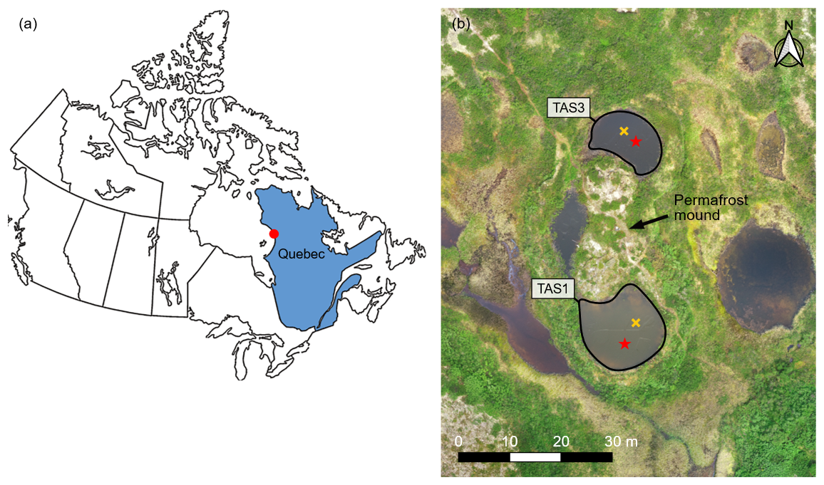
Figure 1 Location map of the Tasiapik Valley: (a) Map of Canada highlighting the study site marked with a red dot, and (b) areal contours of the two lakes under study. The locations of the mooring lines are marked with red stars, while the bubble traps locations are marked with yellow crosses. Aerial photography by Madeleine St-Cyr.

This study quantified GHG emissions from two lithalsa thermokarst lakes in a subarctic region of Canada. Despite being located on the same degrading permafrost mound, the lakes differ in key characteristics: one is more sheltered and humic, while the other is wind-exposed and more transparent. The objectives were to (1) characterise their physicochemical properties, (2) assess the magnitude and diel variation of summer GHG fluxes and (3) explore how seasonal patterns in limnophysical conditions may influence GHG dynamics. We conducted two contrasting summer campaigns in 2022 and 2023 – one during a colder period and the other during a warmer one – focusing on temporal patterns in GHG diffusive fluxes and the magnitude of ebullitive fluxes in 2023. In addition, we continuously monitored water column conditions for 2 yr, alongside hourly meteorological data, enabling extrapolation beyond the flux observation period.

2 Methods

2.1 Study site

The study site (56°33^′28.8^′′ N, 76°28^′46.5^′′ W) is located in the Tasiapik Valley, near the Inuit community of Umiujaq in Nunavik, Quebec, Canada. In the lower part of the valley, the surface deposits are predominantly marine silt, while the upper part consists of a thin layer of littoral sands. Discontinuous permafrost started penetrating the silt unit in the lower valley around 6500 years BP. In the upper valley, the sand layer generally prevented permafrost aggradation, but in areas with a thinner sand layer, the underlying silt froze, leading to the formation of permafrost mounds (Dagenais et al., 2020; Fortier et al., 2020).

The region has a subpolar continental climate, characterised by long winters and short, cool summers. Over the period 1997–2023, the mean annual air temperature was approximately −3 °C. Vegetation in the Tasiapik Valley is highly variable: the upper valley is dominated by lichen-covered mounds surrounded by shrubs, while the lower valley is primarily covered by forested tundra. This diversity of vegetation types highlights the valley's role as an ecotone, a transitional zone between tundra and boreal forest ecosystems. Climate change trends observed in Nunavik indicate that permafrost in the region has been degrading over the past 25 years (Lemieux et al., 2016).

Table 1 Morphometric characteristics of the studied thermokarst lakes, derived from bathymetric maps created in July 2022, along with Secchi depth measurements.

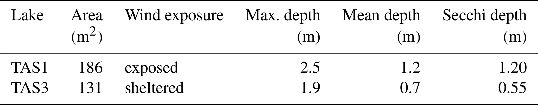
Table 2 Chemical and optical properties of the two lakes surveyed in 2022 and 2023, including the absorption coefficient at 320 nm (a₃₂₀; a proxy for chromophoric DOM), dissolved organic carbon (DOC), specific ultraviolet absorbance at 254 nm (SUVA₂₅₄), total nitrogen (TN), total phosphorus (TP), pH, conductivity, and total suspended solids (TSS). Data are presented for both surface and bottom samples.

NA: not available.

2.2 Lake surveys

We closely monitored two lakes located in the upper valley (Fig. 1), referred to as TAS1 and TAS3 for consistency with previously sampled lakes in the region (unpublished results). Two intensive summer campaigns were conducted: one from 7–16 July 2022, and another from 9–21 August 2023. In addition, the lakes were continuously monitored from October 2021 to August 2023 to study their oxythermal structure. The two shallow thermokarst lakes are situated on a single degrading lithalsa mound, as shown in the bathymetric map (Fig. S1 in the Supplement). Currently, they remain hydrologically isolated due to an underlying silt layer, with their interannual water balance entirely dependent on the ratio of annual precipitation to evaporation (Bussière et al., 2022). Given their shallow depth, water levels fluctuate significantly. In the future, these lakes may merge into a single waterbody. Like other lakes in the region, they are small, shallow and strongly absorb light. Despite their size, they are stratified, with frequent anoxic conditions in bottom waters, similar to other subarctic thermokarst lakes (Matveev et al., 2018).

TAS1 has a surface area of 186 m² (Table 1) and is located on the south side of the permafrost mound, surrounded by shrubs, though it remains relatively exposed to the wind (Fig. 1). In July 2022, its maximum water level was 2.60 ± 0.02 m, slightly decreasing to 2.50 ± 0.02 m in August 2023. Compared to TAS3, TAS1 has lower concentrations of dissolved organic carbon (DOC), CDOM absorption (at 320 nm, a₃₂₀) and total suspended solids (TSS), making it a more transparent lake with a Secchi depth (Z_SD) of 1.20 m. Nutrient concentrations were also high, with total phosphorus (TP) averaging 245 µg L⁻¹ and total nitrogen (TN) 1337 µg L⁻¹, indicating high potential productivity (Table 2).

TAS3 has a surface area of 131 m² and is located on the northern side of the permafrost mound (Table 1, Fig. 1). Surrounded by higher vegetated ramparts, it is shallower and more sheltered from the wind. The average water level fluctuated considerably between the two summer campaigns, reaching 1.80 ± 0.02 m in July 2022 and decreasing to 1.50 ± 0.04 m in August 2023. TAS3 is more humic than TAS1, with twice the DOC concentration and nearly three times the a₃₂₀ values (Table 2). Its TSS level is also three times higher than in TAS1, making it more opaque, with a Z_SD of just 55 cm. Despite these differences, TAS3 exhibited similarly high nutrient concentrations to TAS1 (Table 2).

2.3 Meteorological conditions

To relate oxythermal conditions and GHG fluxes from the lakes to atmospheric conditions, air temperature, wind speed and wind direction were obtained from a meteorological station located 200 m from the main site (CEN, 2024). In addition, local wind speed was measured 0.2 m above the water surface of both lakes during the intensive summer campaigns using DS-2 Sonic anemometer (resolution: 0.01 m s⁻¹, 1°) mounted on a small floating platform. To estimate the roughness length (z₀), we applied the logarithmic wind profile equation using the wind speed measurements taken at 0.2 m above the lakes during the two intensive campaign periods, along with wind speed data from the nearby meteorological station at 10 m height. Calculations were performed under quasi-neutral atmospheric conditions (bulk Richardson number between −0.05 and +0.05), yielding z₀ values of 0.087 m at TAS1 and 0.112 m at TAS3.

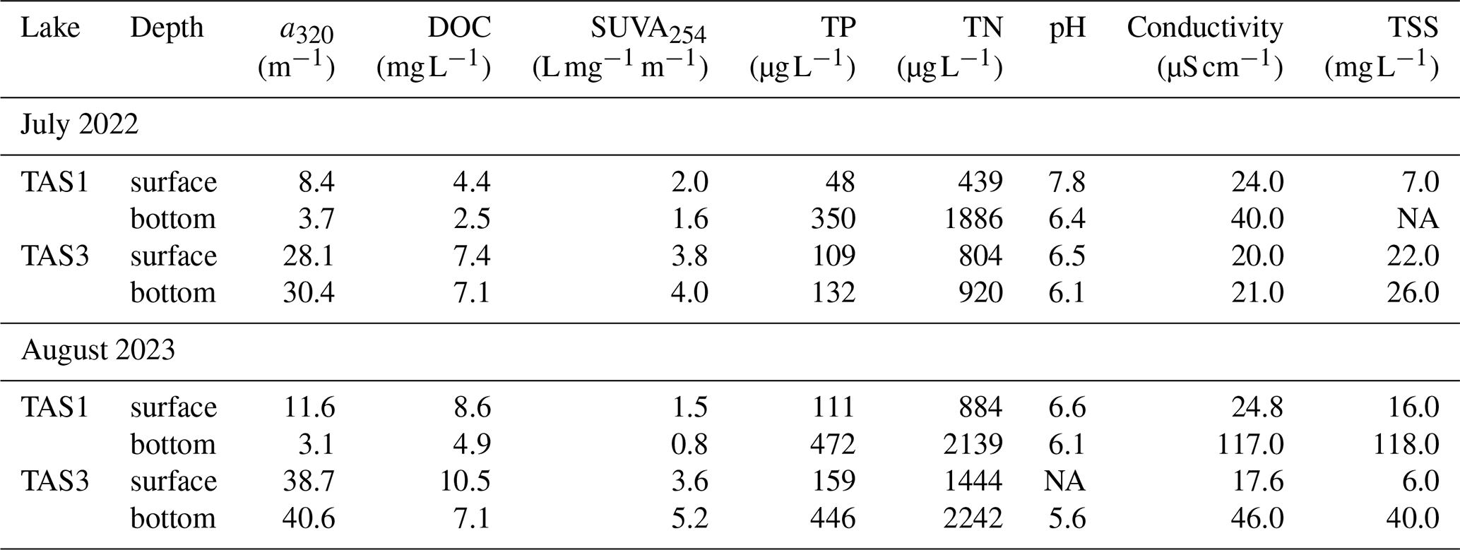
Figure 2 Schematic of the instrumentation deployed in the lakes, including (a) an anemometer mounted on a floating platform (deployed in July 2022 and August 2023), (b) a mooring line equipped with data loggers for continuous oxythermal measurements, (c) a floating chamber connected to an infrared CO₂ analyser (deployed in July 2022 and August 2023), and (d) a bubble trap (deployed in August 2023). Panels (e) and (f) show photographs of TAS1 and TAS3, respectively.

2.4 Limnological profiling

The oxythermal structure was continuously monitored from 7 July 2022 to 21 August 2023 for TAS1 and from 28 September 2021 to 21 August 2023 for TAS3. Dissolved oxygen (PME miniDOT, ± 10 µM, ± 0.1 °C), conductivity (HOBO U24-001, ± 1 µS cm⁻¹, ± 0.1 °C) and pressure (HOBO U20L-01, ± 0.3 % FS, ± 0.44 °C) were recorded at the surface and bottom only. As these loggers also recorded temperature, water temperature was measured at a total of six depths, including four additional depths with HOBO U22-001 (± 0.21 °C) (see logger depths in Table S1 in the Supplement). The submersible automated data loggers were installed on a mooring line at the deepest point of each lake and recorded at hourly intervals (Fig. 2). The buoy was positioned just below the water level to avoid interference from ice during the winter. As the water level was lower in August 2023, the buoy was slightly above the surface, bringing the loggers closer to the surface than in July 2022.

In addition to continuous data collected by the loggers, manual measurements of temperature, dissolved oxygen and conductivity were collected. In 2022, data were recorded using a portable YSI ProODO device (resolution: 0.1 % for dissolved oxygen, 0.1 °C for temperature) and a Seven2Go™conductivity metre (resolution: 0.01 µS cm⁻¹). In 2023, measurements were taken with a ProSOLO device (resolution: 0.1 % for dissolved oxygen, 0.1 °C for temperature, 0.001 mS cm⁻¹ for conductivity).

The buoyancy frequency (N, cycles per hour), which quantifies water column stability, was calculated using the following equation:

$$\begin{array}{}\text{(1)}& N=\sqrt{-{\displaystyle \frac{g\mathrm{d}\mathit{\rho }}{\mathit{\rho }\mathrm{d}z}}}{\displaystyle \frac{\mathrm{3600}}{\mathrm{2}\mathit{\pi }}},\end{array}$$

where g is the acceleration due to gravity (9.81 m s⁻²), ρ is the water density (kg m⁻³) and z is the depth (m). We derived water density from our in situ temperature measurements at the surface and bottom of each lake using the Kell equation (Jones and Harris, 1992). This enabled us to estimate the vertical water density gradient ($\mathrm{d}\mathit{\rho }/\mathrm{d}z$). To quantify the stabilising effect of stratification relative to the destabilising effect of wind-induced shear, the Wedderburn number (W) was calculated as

$$\begin{array}{}\text{(2)}& W={\displaystyle \frac{g\mathrm{\Delta }\mathit{\rho }{h}^{\mathrm{2}}}{\mathit{\rho }{u}_{\ast w}^{\mathrm{2}}L}},\end{array}$$

where Δρ is the density difference across the diurnal thermocline (kg m⁻³), h is the depth of the thermocline (m), ρ is the average water density (kg m⁻³), u_∗w is the friction velocity (m s⁻¹) and L is the length of the lake in the wind direction (m). Values of W > 10 indicate minimal thermocline tilting, 1 < W < 10 indicate partial tilting and W < 1 indicate full upwelling.

2.5 Water chemistry

Several limnological characteristics were measured in each lake during the intensive campaigns, including TP, TN, TSS, pH, conductivity, DOC and CDOM; TP and TN were quantified from unfiltered water samples collected in 50 mL plastic tubes, which were acidified with H₂SO₄ to a pH of 2 and stored at 4 °C until analysis by colorimetry following digestion (details in Bartosiewicz et al., 2016). For CDOM and DOC, water samples were filtered through pre-rinsed polyethersulfone filters (0.2 µm porosity) and stored in amber glass vials at 4 °C. For DOC analysis, 40 µL of pure HCl was added to the vials to adjust the pH to 2 prior to analysis using a Total Organic Carbon analyser (Aurora 1030W, O.I. Analytical) with the persulfate oxidation method. CDOM samples were brought to room temperature within a week of field collection, and absorbance scans were conducted between 200 and 800 nm using a dual beam spectrophotometer (Varian Cary 100 Bio UV-Visible, ± 2 nm) with a 1 cm pathlength quartz cuvette. Null-point adjustment was applied to blank-corrected absorbance spectra using the mean value from 790 to 800 nm. The absorption coefficient at 320 nm (a₃₂₀) was used as a proxy for CDOM concentration. For TSS, water samples were filtered onto pre-burned and pre-weighed glass fibre filters (GF75, 0.7 µm nominal porosity, Advantec). The filters were stored in aluminium foil in the freezer and then dried overnight at 60 °C to determine TSS content.

2.6 GHG flux measurements and estimations

To estimate GHG fluxes, we measured the dissolved concentrations of CO₂, CH₄ and N₂O, as well as CO₂ diffusive fluxes using a floating chamber during the intensive summer campaigns in July 2022 and August 2023. At each lake, measurements were taken over multiple consecutive days across different hours of the day and night. This approach enabled us to reconstruct diel variability in gas fluxes, dissolved gas concentrations and k₆₀₀, yielding between 9 and 13 data points per lake for both intensive campaigns. Ebullitive fluxes of CO₂ and CH₄ were measured at the centre of the lake using an inverted funnel submerged below the water surface; CO₂-equivalent emissions were calculated by applying a global warming potential (GWP): values of 27 for CH₄ and 273 for N₂O, based on a 100-year time horizon, with CO₂ having a GWP value of 1 (IPCC, 2023). All data are presented in Eastern Standard Time (EST).

2.6.1 Dissolved gas concentrations

Dissolved gas concentrations were obtained at the lake surface during each diffusive flux measurement using the headspace method. To account for the accumulation of GHG in the water column, gases were also collected at various depths. In 2022, four profiles were carried out (10, 80, 160 and ∼ 230 cm at TAS1; 10, 50, ∼ 105 and ∼ 155 cm at TAS3). In 2023, two profiles were conducted (10, 120 and 230 cm at TAS1; 10, 70 and 140 cm at TAS3). Water samples were collected from the centre of the lakes using a Van Dorn horizontal sampler (integrating a depth layer of approx. 15 cm). The water was immediately transferred to a 2 L LDPE gas exchange bottle, except at the surface, where it was sampled directly into the bottle. A 30 mL headspace of atmospheric air was created using a syringe connected to an inlet at the bottom of the bottle. The bottle was shaken vigorously for 3 min, and 20 mL of the gaseous headspace was transferred to a 12 mL gas-tight Exetainer vial that had been pre-flushed twice for 10–15 s with nitrogen and vacuumed twice for 3 min. Water temperature was measured at the beginning and end of the exchange process. Atmospheric samples were also taken daily. Gas samples were analysed using a Trace 1310 gas chromatograph (Thermo Fisher Scientific). We used two parallel channels, one with TCD-FID detectors (column HSQ 80/100, MS 5A 80/100) for CH₄ and CO₂, and one with an ECD detector (column HSQ 80/100) for N₂O. Calibration curves were established for CO₂ (up to 10 000 ppm), CH₄ (up to 45 000 ppm) and N₂O (up to 1 ppm). Detection limits were 200 ppm for CO₂, 3 ppm for low CH₄ concentrations, 50 ppm for CH₄ concentrations above 1000 ppm and 0.1 ppm for N₂O. Dissolved CH₄ and CO₂ concentrations were calculated using Henry's law, adjusted for temperature and atmospheric pressure.

2.6.2 Diffusive fluxes

Diffusive fluxes (F_D) of CO₂ ($\mathrm{mmol}{\mathrm{m}}^{-\mathrm{2}}{\mathrm{d}}^{-\mathrm{1}}$) were measured over a full diel cycle during both intensive campaigns (18 measurements in 2022 and 24 in 2023; see Table S2 in the Supplement). These fluxes were obtained by monitoring gas concentration in a floating chamber (area: 0.147 m², volume: 0.0128 m³, including volume of the tube) connected to an infrared gas analyser (EGM4, PP Systems) for approximately 30 min, following the method of MacIntyre et al. (2021):

$$\begin{array}{}\text{(3)}& F_{\mathrm{D}}={\displaystyle \frac{SP{V}_{\text{ch}}}{RT{A}_{\text{ch}}}}D,\end{array}$$

where S is the linear slope of CO₂ (ppm) versus time, P is the atmospheric pressure (Pa), V_ch is the chamber volume (m³), R is the gas constant ($\mathrm{J}{\mathrm{mol}}^{-\mathrm{1}}{\mathrm{K}}^{-\mathrm{1}}$), T is the water temperature (K), A_ch is the chamber surface area (m²) and D is a unit conversion factor to obtain flux values in $\mathrm{mmol}{\mathrm{m}}^{-\mathrm{2}}{\mathrm{d}}^{-\mathrm{1}}$.

To estimate the CH₄ and N₂O fluxes, we used the concentration gradient and the gas transfer velocity (k):

$$\begin{array}{}\text{(4)}& F_{\mathrm{D}}=k(C_{\text{sf}}-C_{\text{eq}}),\end{array}$$

where C_sf is the gas concentration at the water surface (obtained from the headspace method) and C_eq is the aqueous gas concentration in equilibrium with the atmosphere at ambient temperature, both in µM. From this equation, we obtained the k value for CO₂ using direct flux measurements from the chamber and surface water CO₂ concentrations. The corresponding k values for CH₄ and N₂O were computed using the following equation:

$$\begin{array}{}\text{(5)}& k_x=k_{{\mathrm{CO}}_{\mathrm{2}}}{\left({\displaystyle \frac{{\text{Sc}}_x}{{\text{Sc}}_{{\mathrm{CO}}_{\mathrm{2}}}}}\right)}^{-n},\end{array}$$

where Sc_x is the Schmidt number (the ratio of kinematic viscosity to molecular diffusion) for gas x at ambient temperature. The exponent n was set to $\mathrm{1}/\mathrm{2}$ when wind speeds exceeded 3.6 m s⁻¹, and $\mathrm{2}/\mathrm{3}$ when wind speeds were below 3.6 m s⁻¹ (Jähne et al., 1987).

2.6.3 Ebullitive fluxes

Ebullitive fluxes (F_E) of CO₂ and CH₄ were measured in 2023 following the method outlined by Wik et al. (2013). Bubble traps, consisting of inverted funnels with a collection area of 0.23 m², were installed for a total 11 d in both lakes (Fig. 2). The traps were anchored with submerged weights and tied with ropes to fixed shoreline points to minimise movement and drifting. They were positioned near the lake centre to improve representativity of ebullition across the central lake area. N₂O concentrations could not be quantified due to interference from high CH₄ concentrations. The bubble traps were connected to a 140 mL graduated polypropylene syringe and were sampled every 1 to 4 d, depending on the gas accumulation rate. Gas was collected in two replicates (Exetainers) for quantification by gas chromatography. Ebullitive fluxes (F_E) were calculated using the following equation:

$$\begin{array}{}\text{(6)}& F_{\mathrm{E}}={\displaystyle \frac{P{V}_{\mathrm{g}}}{\mathrm{\Delta }t{V}_{\mathrm{m}}A}},\end{array}$$

where P is the partial pressure of the gas (dimensionless), V_g is the total volume of gas in the funnel (m³), Δt is the time interval between two measurements (days), V_m is the molar volume of gas at local air temperature (m³ mol⁻¹) and A is the collection area of the funnel (m²).

3 Results

We first present the annual variations in temperature, oxygen and conductivity observed in the two thermokarst lakes. We then detail the results from the two intensive campaigns, including meteorological conditions, physicochemical profiles and GHG concentrations and fluxes, to examine the magnitude and diel variations during the summer.

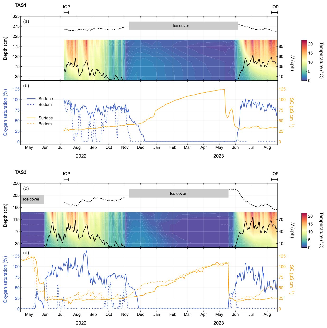
Figure 3 Physicochemical profiles from summer 2022 to summer 2023, showing temperature and buoyancy frequency N for (a) TAS1 and (c) TAS3, with the water surface marked by a black dotted line. Oxygen saturation and specific conductivity (SC) are shown for (b) TAS1 and (d) TAS3. Temperature at the very surface was not measured, as the buoy was positioned below the air–water interface to prevent it from becoming trapped in the ice cover. Nevertheless, winter temperature data suggest that ice may have grown over the buoys, pushing down the mooring and changing the depth of surface sensors, making surface data unreliable. Intensive summer campaign periods are indicated by brackets for July 2022 and August 2023.

3.1 Seasonal profiles

Both lakes had an open-water period of approximately 5 months (June to October) and remained ice-covered for approximately 7 months (November to May) (Fig. 3). Ice-cover duration was determined using Sentinel-2 imagery analysis with an ice detection algorithm through the Google Earth Engine platform, following the approach of Domart et al. (2024). In the winter preceding the 2022 summer campaign, ice began forming on both lakes on 10 November 2021, with ice breakup occurring on 6 June 2022 for TAS1 and 3 June 2022 for TAS3. In the following winter, ice cover formed on both lakes from 10 November 2022 and lasted until 6 June 2023 for TAS1, whereas TAS3 experienced earlier ice breakup on 19 May 2023. During summer, both lakes underwent partial mixing events due to their sensitivity to temperature fluctuations, which caused stratification to weaken rapidly, making the lakes more susceptible to wind-driven mixing. However, complete mixing only occurred in autumn and spring, classifying them as dimictic lakes, although the spring mixing period was notably brief.

At TAS1, the mooring was installed from 7 July 2022 to 21 August 2023, so data from the spring mixing period and the onset of stratification before the 2022 summer campaign are unavailable. However, air temperature data indicate a colder period between late June and early July 2022 (Fig. S2 in the Supplement). This probably led to full oxygenation of the bottom waters by mid-July, as shown by the bottom oxygen logger positioned at 58 cm above the lake bottom (logger depths in Table S1). During the 2022 summer, alternating phases of partial mixing and stratification were observed (Fig. 3a). After a brief period of stratification at the end of July, marked by a peak N value of 64 cph (black curve in Fig. 3a), weakened stratification followed from 4 to 11 August with an N value of 7.5 cph, then stronger stratification by 23 August with N reaching 57.1 cph. Stratification weakened at the end of August, with autumnal mixing beginning by mid-September 2022, followed by reverse stratification from 2 November. Bottom waters turned fully anoxic by 12 November, while surface anoxia was not detected until 9 December. Ion accumulation under the ice throughout the winter increased conductivity to a maximum of 124 µS cm⁻¹ before it dropped on 12 May 2023, probably due to partial ice melt before full ice-off by 6 June 2023. Temperature, conductivity and oxygen profiles suggest that the spring mixing period in TAS1 was extremely brief, lasting only about five days (1–5 June 2023, Fig. 3a and b), but oxygen levels remained near anoxia. Surface oxygen began to increase on 5 June, yet bottom anoxia returned as early as 8 June. Throughout the summer of 2023, thermal stratification persisted, being more pronounced than in 2022 and maintaining bottom anoxia. During the comparable summer period (7 July–21 August), the average N value was 44.6 cph in 2023, compared to 34.4 cph in 2022. Oxygen data from 26 June to 14 July 2023 were deemed unreliable for TAS1 and had to be discarded. However, the thermal structure suggests that anoxic conditions probably persisted during this period (indicated by the red dotted line in Fig. 3b).

At TAS3, the mooring was deployed for nearly 2 yr, from 28 September 2021 to 21 August 2023. During the first recorded winter in 2022, ion accumulation under the ice increased conductivity to a maximum of 123 µS cm⁻¹ before it dropped on 11 May 2022, probably due to partial ice melt. The spring mixing period lasted approximately 23 d (11 May-3 June; Fig. 3c and d), as indicated by conductivity and oxygen data. Thermal stratification established quickly, leading to rapid bottom-water deoxygenation, with complete anoxia occurring within 5 d (Fig. 3c and d), as recorded by the oxygen logger positioned at 44 cm above the sediment layer (Table S1). From 25 June to 10 July, cooler weather allowed brief reoxygenation events to occur (e.g. on 25 June and 4 July; N = 7.5 cph). This was followed by alternating stratification and mixing, with N reaching a maximum of 80.4 cph by late July and a minimum of 17.3 cph at the beginning of August. Strong stratification re-established itself in mid-August, with N reaching 61.6 cph, and intermittent weakening occurred thereafter. Yet bottom waters remained anoxic until the autumn turnover, which started in mid-September. However, bottom-water reoxygenation remained incomplete prior to ice formation. As observed at TAS1, inverse stratification set in on 2 November, leading to full bottom-water anoxia by 7 November, which progressively reached the surface by 27 November. Winter conductivity peaked at 110 µS cm⁻¹ before it dropped on 19 May 2023 following ice breakup. Spring turnover was shorter than in spring 2022 (approx. 13 d, 19 May–1 June 2023, Fig. 3c and d), and stratification redeveloped more quickly, leading to near-instantaneous bottom anoxia by 9 June 2023. As for TAS1, thermal stratification persisted throughout summer in 2023 and was stronger than in 2022 (average N during 7 July–21 August is 50.8 cph vs. 41.2 cph). From 8 July 2023 onward, bottom-water conductivity progressively increased, probably due to the stronger and more persistent stratification in this warmer year.

3.2 Meteorological conditions

Overall, summer 2022 was colder than summer 2023. The average air temperature from mid-June to August was 10.3 ± 4.7 °C in 2022, compared to 13.6 ± 4.3 °C in 2023. In 2022, the average temperature over this period was 0.9 °C lower than normal, whereas in 2023 it was 2.4 °C higher than normal.

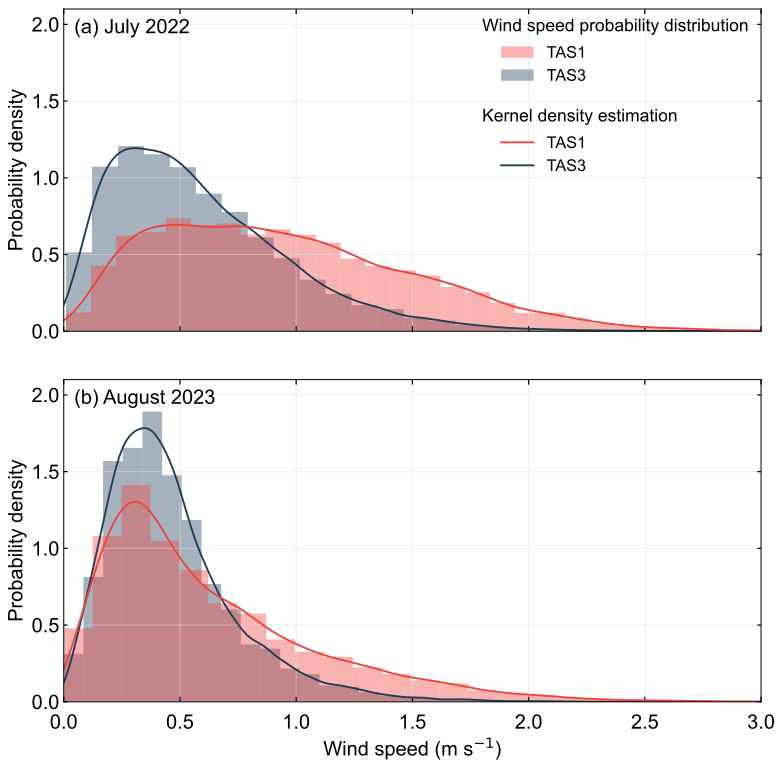
Figure 4 Wind speed probability density function and kernel density estimation at the surface (0.2 m from surface) of TAS1 and TAS3 during the intensive summer campaigns of (a) 7–16 July 2022 and (b) 9–21 August 2023.

Weather conditions varied considerably between the two intensive campaign periods, with July 2022 being significantly colder and windier than August 2023. During the July 2022 campaign, the mean air temperature was 8.8 °C (range: 1.3–23.1 °C), which is 2.7 °C below the July normal of 11.5 ± 5.1 °C. In contrast, August 2023 was substantially warmer, with an average temperature of 14.6 °C (range: 6.6–23.4 °C), which is +2.8 °C above the August normal of 11.8 ± 4.1 °C. The mean wind speed at 10 m height was 4.0 ± 1.7 m s⁻¹ in July 2022, compared to 3.5 ± 2.0 m s⁻¹ in August 2023. Closer to the water surface (0.2 m above), wind speeds were on average 1.4 times higher in 2022 than in 2023. Wind conditions also varied between the sampling sites, with TAS1 experiencing wind speeds 1.5 times higher than TAS3 on average (Fig. 4), as TAS3 is more sheltered by surrounding vegetation and topography. In both years, prevailing surface winds of TAS1 were mainly from the north and west, whereas winds at TAS3 predominantly came from the west (Fig. S3 in the Supplement).

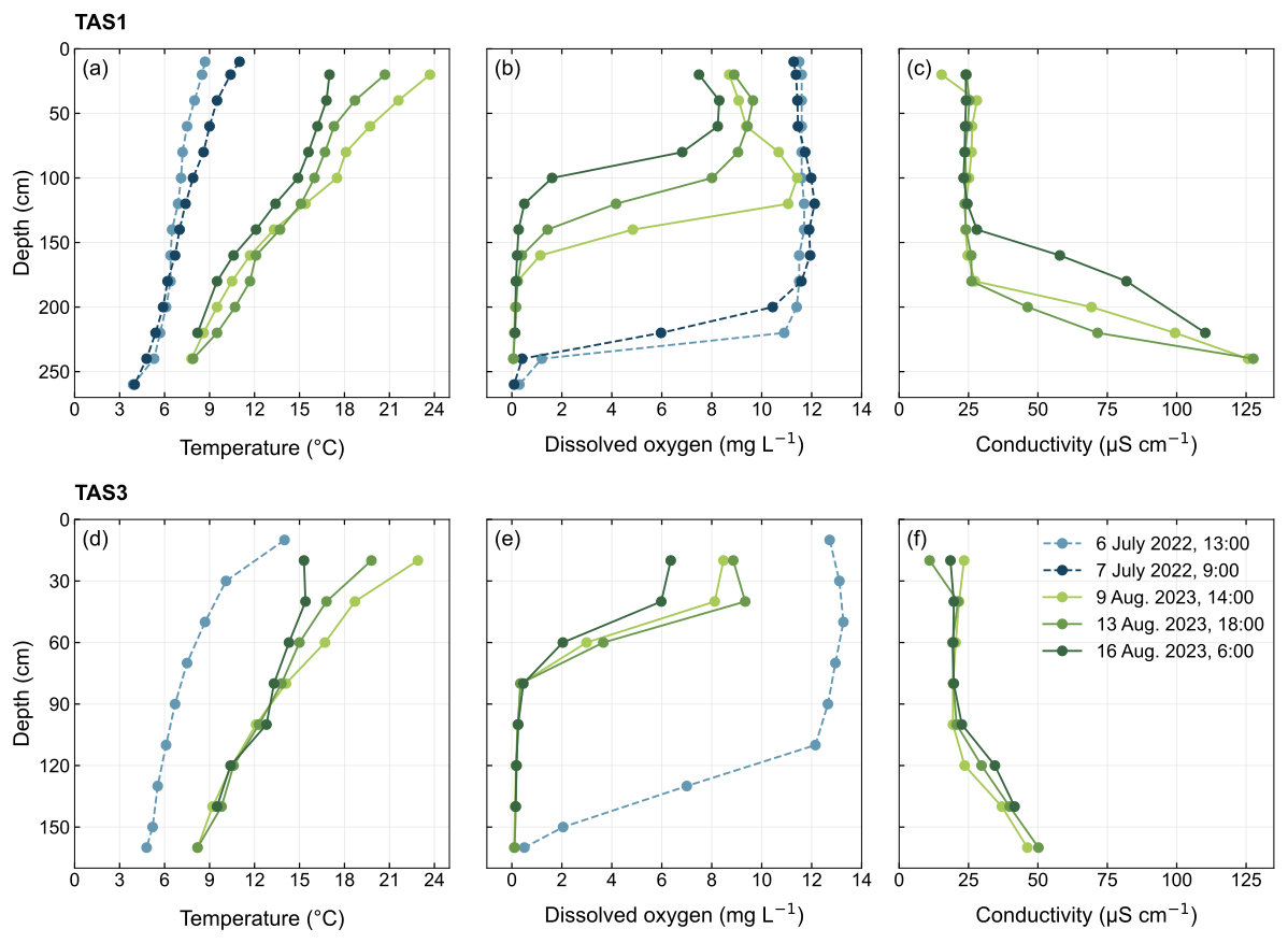
Figure 5 Vertical profiles of temperature, dissolved oxygen and specific conductivity in TAS1 (a–c) and TAS3 (d–f). Dotted lines are profiles in 2022, and solid lines are profiles in 2023.

3.3 Vertical structure of the water column during the intensive sampling periods

Vertical profiles collected manually from the lakes are presented on Fig. 5. Temperature profiles (Fig. 5a and d) indicate that stratification was most pronounced in August 2023, due to warmer conditions and the later timing within the open water season (by 1 month). Despite their shallow depths (2.5–2.6 m at TAS1 and 1.5–1.8 m at TAS3), both lakes exhibited oxygen stratification, with anoxic conditions at the bottom during both observation periods (Fig. 5b and e).

Prior to the 2022 intensive campaign, the lakes had recently undergone a 15 d partial mixing event (25 June–10 July), as indicated by the weaker stratification and bottom-layer reoxygenation at TAS3 (Fig. 3c and d). This mixing event probably released accumulated gases from the previous winter and stratification period. During this time, mixed surface layers were significantly deeper than in August 2023. Based on the rapid decline in dissolved oxygen marking the boundary of the isolated layer, mixed layers extended to 2.1 m at TAS1 and 1.1 m at TAS3 (Fig. 5). These deeper mixed layers allowed a larger portion of the water column to interact with the atmosphere, resulting in greater oxygenation, with levels nearing 100 % saturation (Fig. 5). In TAS3, oxygen supersaturation was observed on the afternoon of 6 July, reaching up to 124 % near the surface and extending down to 0.9 m. However, below the mixed layer, oxygen remained depleted, suggesting the accumulation of GHGs. Despite the small fetch of these lakes (approx. 15 m at TAS1 and approx. 12 m at TAS3), our estimations revealed low Wedderburn numbers (W) during the day (Fig. S4 in the Supplement), indicating susceptibility to mixing as wind increased. At TAS3, W mostly indicated partial thermocline tilting (1 < W < 10) during the day, whereas at TAS1, it generally suggested minimal tilting (>10). By mid-July (from 12 July), as temperature warmed and wind was weaker, values suggested minimal thermocline tilting in both lakes.

In contrast, during the August 2023 campaign, strong thermal stratification prevailed, leading to anoxic bottom waters from early June in both lakes. The mixed layers were much shallower – only 1.0 m at TAS1 and 0.5 m at TAS3. This stronger thermal stratification was reflected in the sharper oxygen concentration gradient, especially at TAS3, and a larger part of the water column that remained anoxic. In addition, the specific conductivity increased considerably with depth, particularly at TAS1 (up to 128 µS cm⁻¹ or total dissolved solids of 123 mg L⁻¹), which contributed to stronger density stratification. For example, temperature accounted for a density difference of 1.796 kg m⁻³ on 13 August, while conductivity contributed approximately to 0.074 kg m⁻³, based on the simplified relationship of ρ = 1000 + 0.000695 TSD kg m⁻³ (Collins, 1987). Our estimations of W mostly indicated partial tilting during the day but minimal tilting at night (reaching up to 10⁸ on 15 August). Episodes of full upwelling (W < 1) were estimated during the day on 11 and 17 August TAS3. Throughout both intensive campaigns, TAS3 consistently showed lower W values, suggesting a greater potential for tilting compared to TAS1.

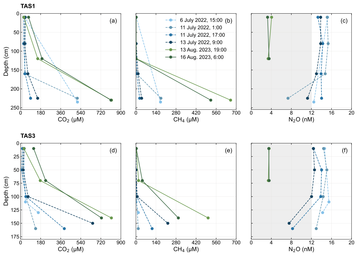
Figure 6 Concentration profiles of CO₂, CH₄ and N₂O from TAS1 (a–c) and TAS3 (d–f). Dotted lines represent profiles from 2022, while solid lines represent profiles from 2023. The shaded area represents the concentrations below atmospheric equilibrium values.

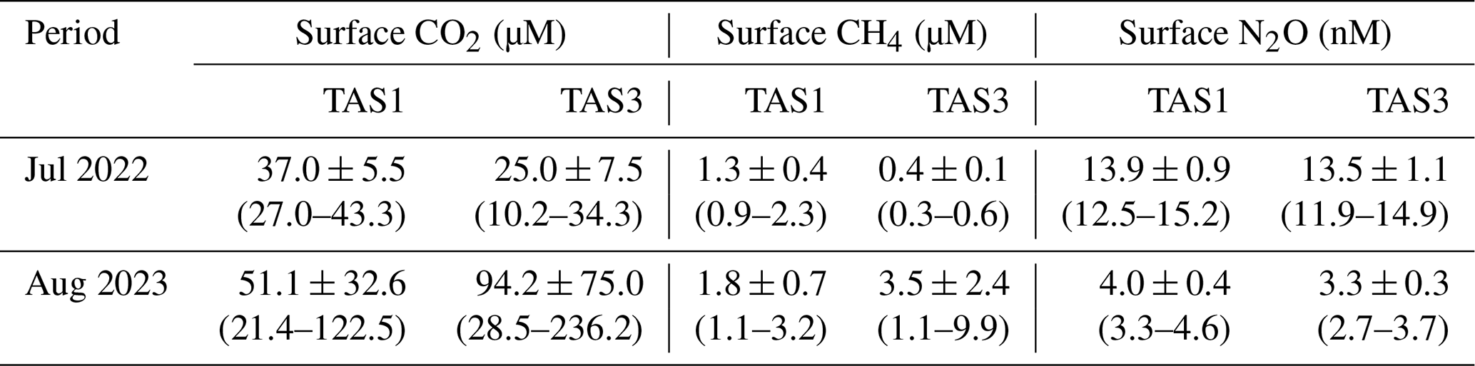
Table 3 Near-surface CO₂, CH₄ and N₂O concentrations measured at TAS1 and TAS3. Values are presented as mean ± standard deviation (min-max). N=10 for 2022 and N=13 for 2023.

3.4 Summer GHG concentrations

During both intensive summer campaigns, the lakes were supersaturated with CO₂ and CH₄ at the bottom but mostly undersaturated with N₂O (Fig. 6). In the July 2022 campaign, increased accumulation of GHGs in the bottom layers resulted in a pronounced vertical gradient of gas concentrations. Specifically, CO₂ concentrations at the bottom were, on average, 11 times higher than at the surface, while the CH₄ gradient was even more pronounced, with bottom concentrations 144 times greater than at the surface on average. In contrast, N₂O concentrations decreased with depth, with surface values on average 1.2 times lower than those in the deeper layers. These gradients resulted in surface gas concentrations that were mostly above air equilibrium for CO₂, CH₄ and N₂O (Tables 3 and S4). To assess gas saturation, we used global atmospheric partial pressure values, which averaged 20.1 µM for CO₂, 0.0034 µM for CH₄ and 12.0 nM for N₂O (grey section, Fig. 6). Moreover, differences in surface dissolved gas concentrations were observed between the two lakes. CO₂ and CH₄ surface concentrations were, respectively, 1.5 and 2.9 times higher at TAS1 compared with TAS3, despite similar bottom concentrations of both gases and a lower pH at TAS3, which could have favoured CO₂ solubility (Tables S5, 2).

During the August 2023 campaign, GHG accumulation in the bottom layers led to a steeper vertical gradient. CO₂ concentrations at the bottom were, on average, 12 times higher than at the surface, while bottom CH₄ concentrations were 223 times higher than at the surface. N₂O bottom concentrations were not available in 2023. These gradients resulted in surface gas concentrations that were strongly above air equilibrium for CO₂ and CH₄ but below air equilibrium for N₂O (Table 3). When comparing the two lakes, CO₂ and CH₄ surface concentrations at TAS3 were approximately twice those found at TAS1, despite lower bottom concentrations at TAS3 (Table S5). This difference was again accompanied by a lower pH at TAS3 (Table 2).

Overall, the lakes accumulated 2.4 times more CO₂ and 5 times more CH₄ at the bottom in August 2023 compared to July 2022. While bottom N₂O concentrations are unavailable for 2023, concentrations in the middle of the water column were already 3 times lower than those observed in 2022. Surface concentrations of CO₂ and CH₄ were also higher in August 2023 compared to July 2022, while N₂O levels were much lower.

3.5 Summer GHG fluxes

In both years, CO₂ and CH₄ exhibited variable fluxes, with emissions predominantly positive, while N₂O fluxes remained consistently close to equilibrium.

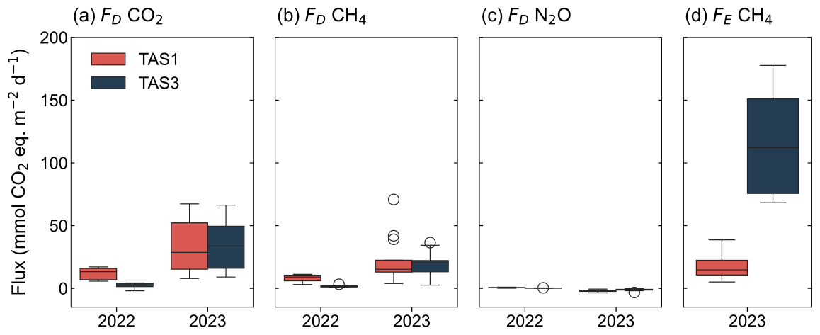
Figure 7 Boxplots of (a) diffusive CO₂ flux, (b) diffusive CH₄ flux, (c) diffusive N₂O flux, and (d) ebullitive CH₄ flux. Fluxes are expressed in $\mathrm{mmol}{\mathrm{CO}}_{\mathrm{2}}\mathrm{equivalent}{\mathrm{m}}^{-\mathrm{2}}{\mathrm{d}}^{-\mathrm{1}}$, assuming a GWP of 27 for CH₄ and 273 for N₂O. Ebullitive flux measurements are only available in summer 2023.

In 2022, CO₂ diffusive fluxes ranged from −2.0 to 17.1 $\mathrm{mmol}{\mathrm{m}}^{-\mathrm{2}}{\mathrm{d}}^{-\mathrm{1}}$, with R² values from the linear regressions averaging 0.94. CH₄ fluxes ranged from 0.1 to 1.1 $\mathrm{mmol}{\mathrm{m}}^{-\mathrm{2}}{\mathrm{d}}^{-\mathrm{1}}$, and N₂O fluxes oscillated around zero, never exceeding 0.0036 $\mathrm{mmol}{\mathrm{m}}^{-\mathrm{2}}{\mathrm{d}}^{-\mathrm{1}}$ (Table S3 in the Supplement). In terms of CO₂-equivalent emissions, CO₂ accounted for the largest portion of average diffusive emissions, contributing nearly 56 % of the total, followed by CH₄ at 41 %, and N₂O at only 3.0 % (Fig. 7). This analysis excludes ebullition, as it was not assessed in 2022. Average diffusive GHG emissions from TAS1 were 5 times higher than those from TAS3, consistent with the higher surface concentrations observed at TAS1 as well as the more turbulent conditions (average k₆₀₀ of 3.5 cm h⁻¹ at TAS1 and 1.9 cm h⁻¹ at TAS3) (Table S6 in the Supplement). One of our k estimates was negative (11 July 2022, 17:15 at TAS3; see Table S2), which can happen near equilibrium due to uncertainties in the measurements. This value was excluded from the analysis.

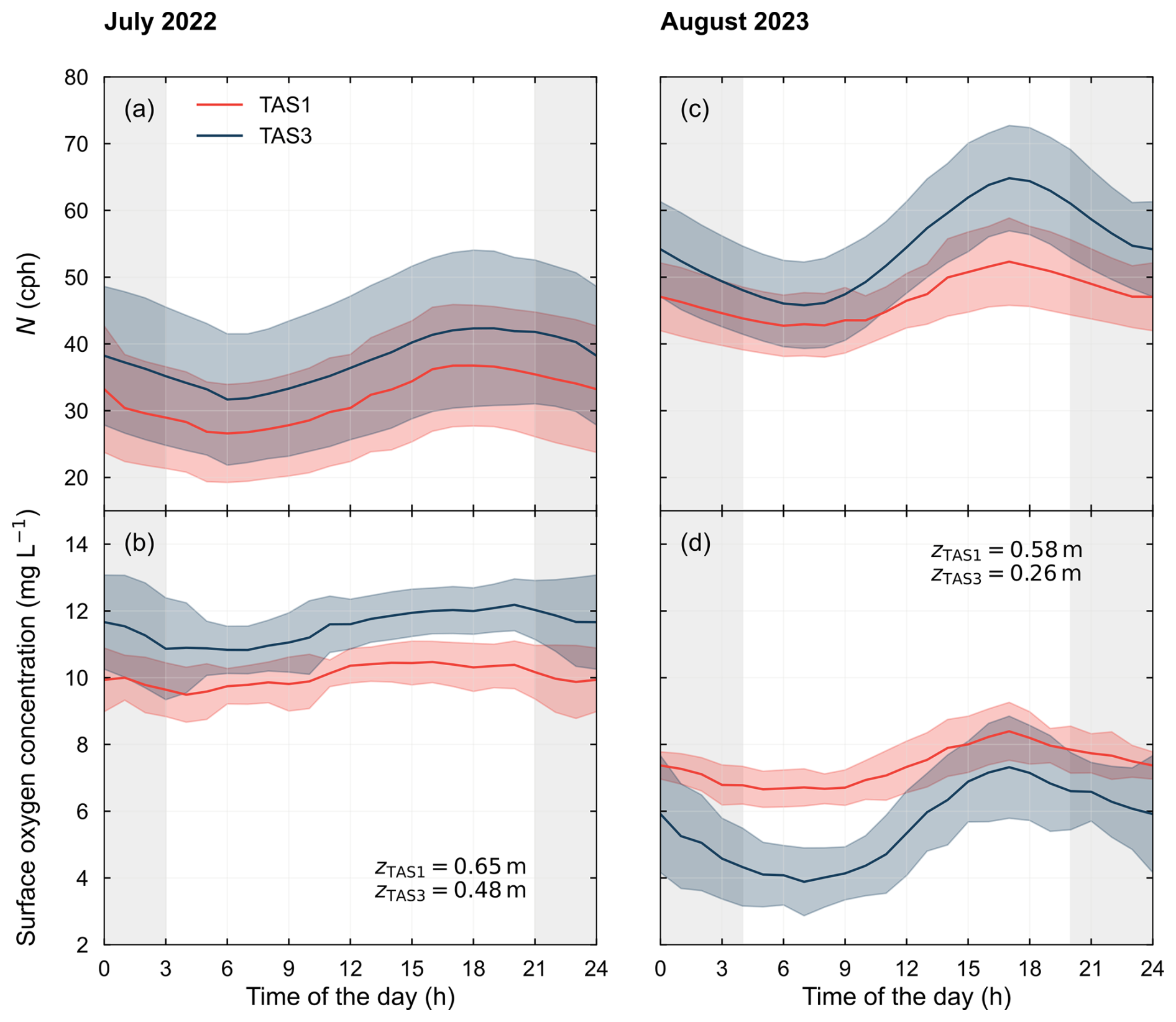
Figure 8 Diel cycles of buoyancy frequency N (a, c) and surface dissolved oxygen at depth z (c, d) for the July 2022 (a, b) and August 2023 (c, d) intensive summer campaign periods. The coloured shaded area represents the standard deviation calculated for each hour of the day based on all available measurements within that hour. The grey shaded area indicates periods of zero solar radiation. Time of day is expressed in EST.

In 2023, CO₂ diffusive fluxes ranged from 7.8 to 67.4 $\mathrm{mmol}{\mathrm{m}}^{-\mathrm{2}}{\mathrm{d}}^{-\mathrm{1}}$, with R² values from the linear regressions averaging 0.99. CH₄ fluxes ranged from 0.3 to 7.2 $\mathrm{mmol}{\mathrm{m}}^{-\mathrm{2}}{\mathrm{d}}^{-\mathrm{1}}$, and N₂O fluxes ranged from −13.2 to −0.7 $\mathrm{mmol}{\mathrm{m}}^{-\mathrm{2}}{\mathrm{d}}^{-\mathrm{1}}$ (Table S3), resulting from the negative gradients at the air–water interface (Fig. 6). Similar to 2022, CO₂ remained the dominant contributor in terms of CO₂-equivalent diffusive emissions, comprising 64 % of total emissions, while CH₄ contributed 39 %, and N₂O mitigated total emissions by 4 % (sink; Fig. 7). Despite total diffusive fluxes being similar between TAS1 and TAS3 in 2023, surface concentrations of CO₂ and CH₄ were lower at TAS1 (Table 3). This difference is due to the more turbulent conditions at TAS1 (average k₆₀₀ of 5.7 cm h⁻¹), which increased the overall emissions compared with those at TAS3 (average k₆₀₀ of 2.9 cm h⁻¹; see Table S6). Significant CH₄ ebullitive fluxes were recorded at both sites, ranging from 0.5 to 18.1 $\mathrm{mmol}{\mathrm{m}}^{-\mathrm{2}}{\mathrm{d}}^{-\mathrm{1}}$, while CO₂ ebullitive fluxes remained negligible (Table S3). At TAS1, CH₄ ebullitive fluxes were slightly lower than diffusive fluxes, whereas at TAS3, they were more than 6 times higher than diffusive fluxes on average. Consequently, ebullition accounted for 70 % of total emissions at TAS3, primarily driven by CH₄.

Overall, GHG emissions were higher during the intensive campaign period in August 2023 compared to July 2022. The mean diffusive flux of CO₂ was 4.7 times higher, while CH₄ fluxes were almost 4 times greater. This increase is attributed to higher surface concentrations of both gases (Table 3) and greater turbulence, as indicated by the higher k values in 2023 (Table S6). These conditions were reflected in the N₂O fluxes, which were consistently negative in 2023, although this flux remains negligible relative to the total flux.

3.6 Summer diel cycles in stratification and diffusive fluxes

During both intensive summer campaigns, clear diel cycles in the buoyancy frequency (N) and dissolved oxygen (DO) were observed (Fig. 8), as indicated by the data collected from the moorings. Although temperature was more variable in 2022 (Fig. S5 in the Supplement), peaks in both N and DO typically occurred in the evening (around 18:00; all times are expressed in EST), while the lowest values were recorded in the morning (around 07:00). The grey shaded area in the figure indicates periods of zero solar radiation. All data are presented in Eastern Standard Time (EST).

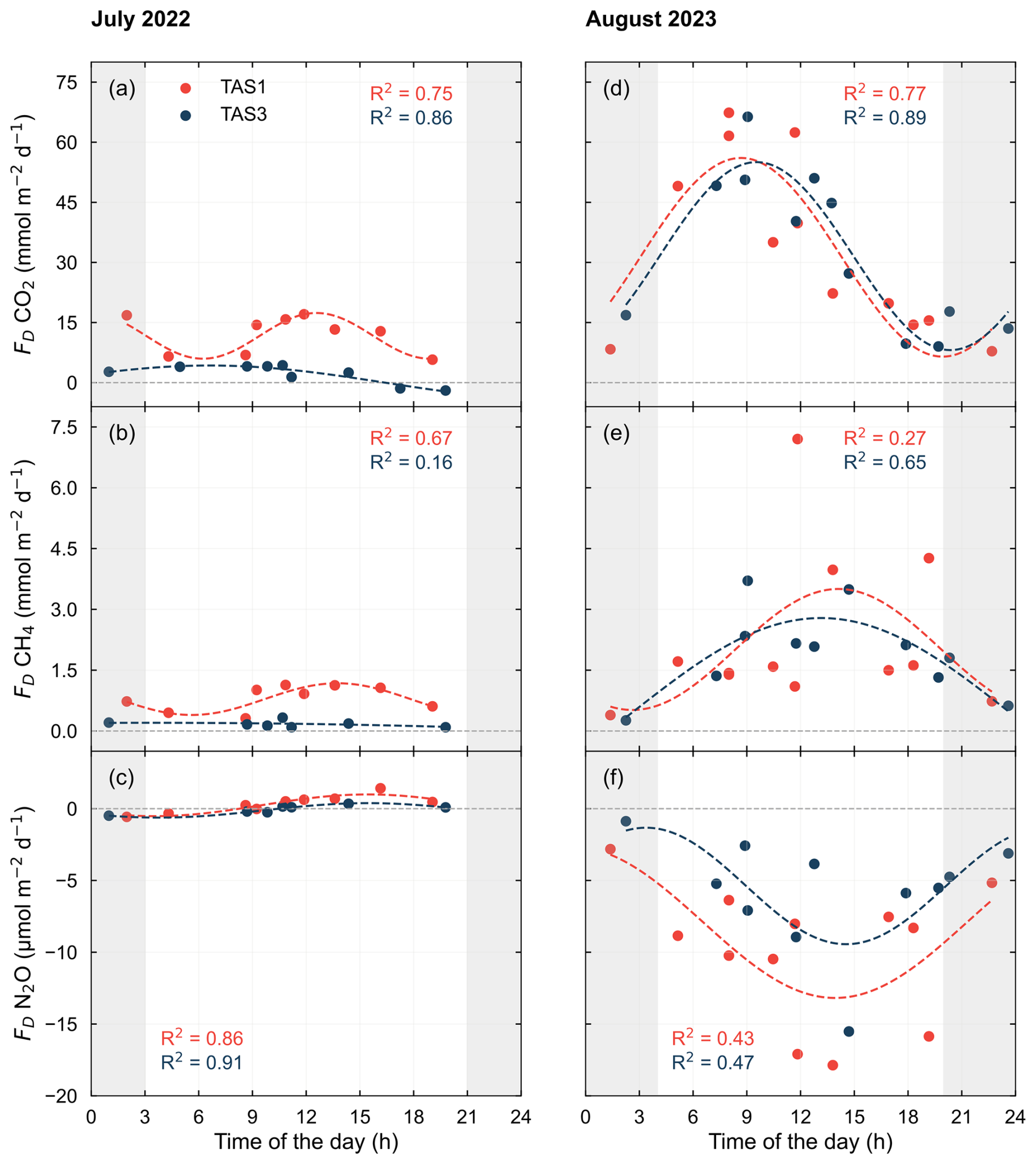
Figure 9 Diel cycles of CO₂ (a, d), CH₄ (b, e) and N₂O (c, f) diffusive fluxes for the July 2022 (a–c) and August 2023 (d–f) intensive summer campaign periods. CO₂ fluxes were measured directly with the floating chamber, while CH₄ and N₂O fluxes were obtained by applying the k values derived from CO₂ fluxes to their respective concentrations. The grey dotted line represents atmospheric equilibrium, and the grey shaded area indicates periods of zero solar radiation. Although the data are presented on a diurnal cycle, the measurements were taken over a 2 week period (see Table S2). Coloured dotted lines represent sine-fitted trend lines. Time of day is expressed in EST.

Measurements of CO₂ fluxes, dissolved gas concentrations and k₆₀₀ over multiple consecutive days across different hours allowed us to reconstruct diel variability for both intensive campaigns (Fig. 9). In 2022, no discernible diel patterns were observed in either the surface concentrations (Fig. S6a–c in the Supplement), the gas transfer coefficient (Fig. S7a in the Supplement) or the diffusive emissions of CO₂, CH₄, and N₂O (Fig. 9a–c). However, in 2023, distinct diel cycles for diffusive emissions of all three gases emerged (Fig. 9d–f), along with the gas transfer coefficient in both lakes, with higher k values observed during the daytime (Fig. S7b). CO₂ fluxes and concentrations exhibited a morning peak between 06:00 and 12:00, followed by a decline to their lowest levels during the evening and night (18:00–03:00; Fig. 9d). CH₄ concentrations were generally higher in the morning and lower at night, though this pattern was less pronounced at TAS1, where concentrations were slightly higher during the day. CH₄ fluxes also displayed a clear diel pattern, with daytime peaks between 09:00 and 18:00 and minima recorded at night (21:00–03:00; Fig. 9e). While N₂O concentrations showed no clear diel trend (Fig. S6d–f), N₂O fluxes displayed similar variability to CH₄, with negative fluxes peaking during the day (09:00–18:00), approaching equilibrium at night (21:00–03:00; Fig. 9f).

4 Discussion

The results highlight that GHG emissions from small thermokarst lakes are highly sensitive to interannual variations in meteorological conditions. In this section, we discuss the physicochemical characteristics specific to thermokarst lakes, the summer patterns of dissolved gases and fluxes and the role of diel and seasonal variability in upscaling lake emissions. Finally, we reflect on the limitations of the study.

4.1 Physicochemistry

Thermal stratification in both lakes in summer, despite their shallow depth (< 3 m), reflects strong near-surface absorption of solar radiation driven by low water clarity as well as sheltering from winds. Stratification was more persistent in 2023, coinciding with warmer air temperatures, leading to persistent bottom anoxia. Partial mixing during nighttime cooling eroded this stratification, bringing oxygen-depleted water from deeper layers to the surface, causing surface waters to remain continuously undersaturated with respect to oxygen that summer (Fig. 8). The subsurface oxygen peak, such as the 119 % saturation at 100 cm below water surface at TAS1 on 9 August at 15:00, suggest photosynthesis and resistance to mixing. In contrast, 2022 saw cooler, windier conditions that allowed partial mixing and brief bottom reoxygenation. However, oxygen levels quickly returning to anoxic conditions as stability increased (Fig. 3) suggest a high oxygen demand from deeper water and lake sediments. Oxygen supersaturation observed near the surface in TAS3 reflects active photosynthesis and efficient mixing within the surface layer. Overall, the differences observed between the two summers underscore the sensitivity of small lakes to interannual variations in meteorological conditions. Warmer conditions, as observed in 2023, can lead to a rapid onset of spring thermal stratification, potentially preventing the release of gases accumulated during the winter and maintaining a hypoxic lower water column, which allows methane to accumulate more rapidly (e.g. Cortés and MacIntyre, 2020).

Lake-specific features further influenced stratification strength and vertical mixing. TAS3, with a₃₂₀ values more than 3 times higher than at TAS1 in both years (Table 2), absorbed more solar radiation and consistently developed stronger density gradients and shallower mixed layers. In addition, TAS1 experienced more frequent partial mixing (Fig. 3b) and signs of deeper oxygen penetration (Fig. 5b), although differences in sensor placement may have influenced observations, with the logger positioned 58 cm above the bottom at TAS1 compared to 44 cm at TAS3.

Finally, the discrepancy in ice-off dates between lakes in 2023, with TAS3 melting approximately 2.5 weeks earlier than TAS1, suggests that the ice detection algorithm, which relies on Sentinel-2 imagery, may have missed the actual breakup at TAS1 due to the small size of the lakes and the spatial resolution of 10 m of the imagery. Conductivity data suggest that partial ice melt at TAS1 occurred in mid-May, though not enough to reoxygenate the water, unlike at TAS3. This discrepancy could be due to the higher concentration of CDOM in the ice at TAS3, which could have enhanced sunlight absorption and accelerated melting.

4.2 Summer dissolved gases

The increased supersaturation of CO₂ and CH₄ at the bottom of both lakes during the warmer August 2023 intensive campaign, coupled with the undersaturation of N₂O, underscores the key role of thermal stratification in regulating gas concentrations and vertical gradients. The observed steeper vertical gradients suggest that stratification limited gas evasion to the atmosphere due to reduced mixing and prolonged isolation of the hypolimnion (Fig. 6). Moreover, the rapid onset of thermal stratification after ice-cover loss in 2023 (Fig. 3) probably trapped some dissolved gases accumulated during the winter. The increased bottom concentrations of CO₂ and CH₄ in 2023 may also reflect heightened microbial activity and organic matter decomposition in the hypolimnion driven by higher temperatures (see below). While bottom N₂O data were unavailable in 2023, the lower mid-water column N₂O concentrations (Fig. 6) suggest that the expanded anoxic water column created favourable conditions for N₂O consumption (Beaulieu et al., 2014), resulting in negative fluxes.

The greater accumulation of GHGs in the lower layers of both lakes in 2023, along with a shallower mixing layer, increased the potential for GHG transport to the surface during mixing and penetrating convection. This, in turn, enhanced both the variability and magnitude of surface GHG accumulation compared to 2022. Notably, the higher GHG concentrations at the surface of TAS3 in 2023 may reflect deeper diurnal mixing, as suggested by lower W values during the day (1 < W < 10). Since the mixing layer at TAS3 is shallower than at TAS1 (Fig. 5), wind can more easily disrupt stratification. In addition, the steeper oxygen gradient in this lake may promote CH₄ production by extending anoxic conditions over a larger portion of the water column. Although photosynthesis and respiration influence CO₂ concentrations through daytime consumption and nighttime production, the large variability in surface concentrations suggests that these processes alone cannot fully explain the observed differences.

The disparities in surface gas concentrations between the two lakes and intensive campaign periods highlight the complexity of the processes governing gas dynamics in thermokarst lakes. Overall, the enhanced GHG accumulation observed during the warmer summer suggests that future climate warming could further amplify GHG buildup in stratified lakes, generating larger seasonal variations.

4.3 Summer GHG fluxes

Studies presenting GHG fluxes from thermokarst lakes and ponds remain scarce. To compare our results with other studies, Table 4 lists the reported CO₂ and CH₄ flux from different regions. This non-exhaustive list includes only studies that explicitly identify water bodies formed through thermokarst activity.

In general, our diffusive flux aligns with the range of CO₂ and CH₄ fluxes reported for lakes and ponds in the region. Our results show that under warm and stratified conditions (August 2023), the total diffusive flux was four times higher than under colder conditions (July 2022). However, N₂O fluxes were notably lower during this period (higher but negative). Despite the high GWP of N₂O (GWP of 273), its uptake had minimal impact on the total GHG fluxes. This pattern is consistent with findings from Davidson et al. (2024), where a shallow eutrophic lake in Denmark acted as a N₂O sink in late summer. Similarly, Bartosiewicz et al. (2016) reported a negligible contribution of N₂O to total GHG emissions from a small, shallow lake in southeastern Canada, where concentrations often remained low or even undersaturated during a heat wave. On the other hand, greater exposure to wind (as in TAS1) resulted in higher k values and higher fluxes, indicating that GHG dynamics can differ significantly between nearby lakes.

Table 4 Reported CO₂ and CH₄ fluxes from thermokarst lakes and ponds. Negative values represent uptake from the atmosphere. N_b is the number of waterbodies studied. Type of permafrost are continuous (C), discontinuous (D) and sporadic (S). Methods for acquiring diffusive flux are chamber (CH), headspace equilibration (HS), sensors measuring concentration directly in the field (SR), bubble traps (BT) and wind models (WM).

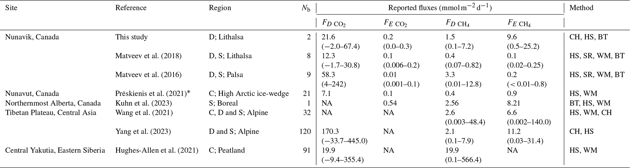
^∗ Kettle lakes in Prėskienis et al. (2021) were later identified by Coulombe et al. (2022) as glacial thermokarst lakes and thus were included in the average grouping ice-wedge trough ponds, ice-wedge thermokarst lakes, and glacial thermokarst lakes. NA: not available.

The high CH₄ ebullition fluxes recorded are consistent with findings from other studies documenting large CH₄ ebullition flux during the stratified phase (Davidson et al., 2024). The values observed at TAS3, particularly humic and sheltered, are among the highest reported for CH₄ ebullition in Nunavik (Table S3). However, even higher CH₄ ebullition fluxes have been reported from Arctic thermokarst lakes (Table 4). In terms of CO₂-equivalent emissions, CH₄ ebullition at TAS3 contributed 70 % of total emissions, compared to 25 % at TAS1. The exact reasons for the higher ebullition rates at TAS3 remain unclear, but several factors may contribute. One possibility is its higher organic content, with bottom DOC levels nearly three times higher than at TAS1 (Table 2), potentially reflecting a higher microbial productivity. Plankton was abundant in TAS3 (though not analysed), and the presence of dense shrub cover along its shores suggests that falling leaves contribute organic material to the water column and sediment, fuelling methanogenic activity (Heslop et al., 2015). However, we acknowledge that our estimates of CH₄ ebullition were based on measurements taken from a single funnel deployed at the centre of the lake. This approach restricts the spatial representativeness of the results, especially since ebullition is known to be highly heterogeneous, with localised hotspots often occurring near lake edges or thawing permafrost zones (Wik et al., 2011; Kuhn et al., 2023). This spatial limitation may partially explain the differences observed between the lakes. Future studies should therefore aim to deploy multiple bubble traps across various lake zones to capture this heterogeneity and better constrain whole-lake ebullition estimates.

While both intensive campaign periods occurred during the summer season, we acknowledge that they were conducted at different times, with the 2023 campaign occurring later in the season. Beyond the overall differences in environmental conditions between both summers – 2022 being colder than 2023 – the timing of sampling may have captured distinct seasonal phases. Late summer is typically characterised by a warmer water column and greater accumulation of GHGs at the bottom due to prolonged stratification throughout the season (Prėskienis et al., 2021).

4.4 The importance of diel variability in upscaling emissions

Estimates of GHG emissions from lakes often rely on daytime measurements, but our findings indicate that this approach can significantly overestimate total 24 h fluxes. Numerous studies have also reported diel variability in subtropical lakes (Zhao et al., 2024), boreal and temperate lakes (Sieczko et al., 2020; Erkkilä et al., 2018; Podgrajsek et al., 2014; Martinez-Cruz et al., 2020), subarctic lakes (Jammet et al., 2017) and glacial lakes (Eugster et al., 2022), as well as across multiple sites in the Northern Hemisphere (Golub et al., 2023). In 2023, the pronounced diel pattern in surface gas concentrations and k led to significantly higher daytime (09:00–17:00) diffusive fluxes: 47 % higher for CO₂, 95 % for CH₄, and 75 % for N₂O (negative fluxes for N₂O; Fig. 9). Notably, this pattern was not observed in July 2022, probably due to the colder weather and weaker stratification following a recent mixing event, which may have resulted in gas venting (Fig. 3). The drivers of diel GHG emission patterns are multifaceted, involving both physical (mixing patterns) and biological factors (production vs. consumption rates), though the latter were not explored in this study. For instance, the decline in surface oxygen observed approximately 3 h after sunrise (Fig. 8) may be attributed to increasing morning winds, which promote vertical mixing, combined with ongoing respiration that outpaces photosynthesis early in the day.

Our results show that the high morning CO₂ fluxes were primarily driven by elevated gas concentrations in the upper water column, illustrated by the significant correlation between flux and departure from saturation (r = 0.49, p =  0.018). The higher morning CO₂ concentrations coincided with weaker stratification and lower oxygen levels at that time (Figs. S6d and 8c, d). The rapid decrease from noon was probably due to increased photosynthetic activity driven by solar radiation (which peaks around 12:00; Fig. S5) and reduced CO₂ solubility as daytime temperatures rose. This pattern aligns with findings from Arctic thermokarst lakes (Prėskienis et al., 2021), where nighttime respiration and daytime photosynthesis, along with nighttime convective mixing, were suggested to concurrently drive CO₂ and O₂ dynamics by bringing GHG-enriched, oxygen-depleted water from deeper layers to the surface (Anthony and MacIntyre, 2016). Similarly, elevated morning CO₂ concentrations have been reported in a boreal humic lake, where surface concentrations were strongly influenced by the stability of stratification (Huotari et al., 2009).

Wind-induced turbulence played a dominant role in controlling fluxes of CH₄ and N₂O, as these gases were more closely linked to k patterns (r = 0.78, p < 0.001; r = −0.98, p < 0.001 for CH₄ and N₂O, respectively), with their surface concentrations remaining relatively stable. However, CH₄ in TAS3 followed a pattern similar to CO₂, highlighting the need for additional measurements to better resolve these diel patterns. Wind-driven dynamics contributing to higher daytime fluxes have also been reported in boreal lakes (Sieczko et al., 2020). These differing dynamics caused CH₄ and N₂O fluxes to peak later in the day compared to CO₂. This contrasts with findings from Eugster et al. (2020), who reported elevated CO₂ and CH₄ fluxes at night (02:00–06:00) in a deep glacial lake, and Podgrajsek et al. (2014), who observed high CH₄ fluxes during the night and early morning (00:00–08:00) in a boreal lake, both coinciding with periods of strongest surface cooling and convection. These results highlight the importance of conducting full 24 h sampling in order to accurately capture GHG emissions from lakes, not only in biologically productive systems, but also in high-latitude thermokarst environments. Despite their small size and shallow depth, these lakes exhibit pronounced diel patterns in stratification and oxygen dynamics, demonstrating that GHG fluxes are largely driven by physical processes. Furthermore, the distinctive light regimes of the Arctic and sub-Arctic regions, characterised by prolonged daylight hours, could intensify stratification during the summer. This emphasises the importance of considering latitude-specific dynamics when evaluating lake GHG budgets.

4.5 Larger-scale estimates and limitations

While our GHG flux measurements are limited to two intensive summer campaigns, we recognise that emissions from thermokarst lakes can vary substantially beyond these short observation windows. In particular, the accumulation of CO₂ and CH₄ in bottom waters during summer and winter stratification may lead to substantial emissions during spring and autumn turnover events. To explore the potential scale of these seasonal variations, we performed an indicative extrapolation of diffusive GHG fluxes using seasonal limnophysical data and dissolved gas concentrations measured in the water columns during summer. The methodological approach and detailed results are listed in Tables S7–S9 in the Supplement) and should be interpreted with caution given the simplifying assumptions and lack of direct flux measurements outside summer.

The larger-scale estimate analysis suggests that GHG fluxes may peak during spring and autumn, particularly at TAS3, where stronger stratification allowed for greater gas buildup at the bottom. CH₄ was the dominant contributor to these estimated peak fluxes when mixing probably released stored gases. The larger GHG fluxes estimated during the summer of 2023 compared to summer 2022 reflects enhanced stratification and intensified decomposition processes, leading to greater accumulation and subsequent release of CO₂ and CH₄. While we were unable to estimate k during the autumn 2023 and spring 2024 periods, it is likely that fluxes would have been substantially higher due to the higher buildup of GHG at the bottom (Table S8 in the Supplement). Overall, these findings emphasise the potential magnitude of emissions outside the summer period and highlight the importance of monitoring GHG fluxes year-round to gain a deeper understanding of the dynamics and drivers behind seasonal emission patterns.

Several factors should be considered to improve the accuracy of GHG flux estimates. First, under calm conditions, microstratification can slow the vertical exchange of gases even within the top few centimetres of the water column. Aurich et al. (2025) demonstrated that CO₂ concentrations may vary significantly between 5 and 25 cm depth during windless periods, with the surface being supersaturated. When quantifying gas concentration with the headspace method, water is typically collected from the upper 10–20 cm, which could overestimate concentrations at the actual surface during warm, calm periods, potentially inflating flux estimates when applying a gas transfer model. In contrast, all measurements in the present study were conducted at the lake centre, which may have led to an underestimation of fluxes. Previous studies, such as Kuhn et al. (2023), have shown that diffusive fluxes near the edges can be significantly higher (twice in their study) than at the centre. Finally, with only one funnel used per lake to measure ebullition, we may have missed localised high-ebullition sites, particularly near the edges, despite the lakes being very small. For instance, Kuhn et al. (2023) reported CH₄ ebullition fluxes up to four times higher at the thawing edges of thermokarst lakes compared to the lake centre.

5 Conclusions

In this study, two thermokarst lakes – one more humic and sheltered and the other more transparent and wind-exposed – were monitored for nearly 2 yr, with continuous measurements of temperature, oxygen and conductivity. These long-term observations were complemented by GHG flux and concentration measurements from two intensive summer campaigns – one colder and the other warmer – to quantify emissions and their variability. The thermokarst lakes were significant emitters of CO₂ and CH₄, with lake N₂O uptake only minimally offsetting these emissions. Our results show large temporal variations in GHG fluxes during the warm intensive campaign in 2023, with peak CO₂ fluxes occurring in the morning and peak CH₄ and N₂O fluxes observed later in the day. The differences observed between the warmer and the cooler intensive campaigns were partly due to the mixing regime and the accumulation of dissolved gases in the water column. Stratification allowed for the buildup of dissolved GHGs, which were then brought to the surface during nighttime cooling and mixing, subsequently released to the atmosphere as wind speeds rose. Notably, ebullitive CH₄ fluxes were predominant in the more humic and sheltered lake, which received organic inputs from leafy shrubs, illustrating the potential differences between two adjacent lakes. While our seasonal flux estimates suggest that emissions may peak in autumn and spring, highlighting the role of GHG storage and release in stratified water bodies, these remain speculative, as no direct seasonal GHG measurements were conducted. This highlights the importance of long-term monitoring that accounts for both seasonal and diel patterns in emissions, alongside the environmental factors that regulate the efficiency of lake mixing and GHG production and consumption.