Marine heatwaves deeply alter marine food web structure and function

Marine heatwaves (MHWs) have become longer, more frequent and more intense in recent decades. MHWs have caused large-scale ecological impacts. This includes coral bleaching; mass mortality of seagrass, fishes and invertebrates; and shifts in the abundance and distribution of marine species. However, the implications of these MHW-induced impacts on marine species for the structure and functioning of marine food webs are not clearly understood. In this study, we use the EcoTroph-Dyn ecosystem modelling approach to examine the impacts of MHWs occurring during the year's warmest month on the trophodynamics of marine ecosystems. EcoTroph-Dyn represents marine ecosystem dynamics at a spatial resolution of 1° longitude by 1° latitude and a temporal resolution of 15 d. We applied the model to simulate changes in trophodynamic processes, energy transfer and ecosystem biomass using daily temperature and monthly net primary production (NPP) data that were derived from satellite observations from 1998 to 2021. We compared and contrasted the simulated changes in biomass by trophic level, with results generated from temperature and NPP time series that had been filtered to remove MHWs. Our results show a significant decline in biomass between 1998 and 2021, specifically caused by MHWs. For example, in the northeastern Pacific Ocean, our model simulated an MHW-induced decline in biomass of 8.7 % ± 1.0 (standard error) from 2013 to 2016. Overall, MHW-induced biomass declines are more pronounced in the Northern Hemisphere and Pacific Ocean. Moreover, the MHW-induced declines in high trophic-level biomass were larger than in lower trophic levels and lasted longer post-MHW. Finally, this study highlights the need to integrate MHWs into modelling the effects of climate change on marine ecosystems. It shows that the EcoTroph approach, and especially its new dynamic version, provides a framework for understanding more comprehensively the implications of climate change for marine ecosystem structure and functioning.

1 Introduction

Over the last century, marine heatwaves (MHWs) – defined as a period of more than 5 d of anomalously warm sea surface temperatures (SSTs) exceeding a specific threshold, typically determined by natural climatological variations – have increased in frequency, duration and intensity (Frölicher and Laufkötter, 2018; Oliver et al., 2018). Between the 1920s and the 2010s, their duration and frequency increased by 17 % and 34 %, respectively, resulting in more than a doubling of the number of MHW days at a global scale (Oliver et al., 2018). Since the 2000s, MHWs that are spatially and temporally extensive have been recorded in the world oceans, such as the North Pacific MHW (“the Blob”) in 2013–2016 (Bond et al., 2015; Cavole et al., 2016), the Mediterranean Sea in 2003 and the 2022 MHW (Garrabou et al., 2009, 2022), the Western Australia MHW in 2011 (Pearce et al., 2011) and the Tasman Sea MHW in 2015–2016 (Oliver et al., 2017).

Marine ectotherms' physiological functions are directly affected by ocean temperature changes that are closely related to impacts on their body temperature (Guibourd de Luzinais et al., 2024; Pörtner and Farrell, 2008). These species are adapted to perform optimally at a range of body temperatures, with upper and lower temperature limits within which they can survive (Pörtner and Farrell, 2008). When environmental temperatures exceed the temperature optima, e.g. during MHWs, the organism is stressed, leading to functional constraints and declines in performance (Pörtner and Farrell, 2008). Particularly, abnormally high temperatures during MHWs often exceed organisms' thermal limits, impacting their distribution, growth and survival (Guibourd de Luzinais et al., 2024; Smale et al., 2019; Smith et al., 2023). Moreover, the impacts of MHWs at the population level have cascading effects at the community and ecosystem levels. For example, MHW-induced declines in phytoplankton biomass and diversity have led to significant changes in zooplankton and other marine invertebrate diversity and biomass (Cavole et al., 2016). MHWs cause coral bleaching that also impacts coral reef ecosystems (Garrabou et al., 2009, 2022; Pearce et al., 2011). Range shifts driven by MHWs result in the “tropicalisation” of fish communities (Wernberg et al., 2016). Ultimately, MHWs result in the mass mortality of fish and invertebrates, modifying ecosystem functioning (Cannell et al., 2019; Cavole et al., 2016; Collins et al., 2019). However, these ecological impacts of MHWs are not ubiquitous and vary largely between MHW events, species and ecosystems (Fredston et al., 2023; Oliver et al., 2021; Pershing et al., 2018; Smale et al., 2019; Smith et al., 2023).

The ecological impacts of MHWs have predominantly been studied using laboratory experimentations, analyses of ecological time series and numerical modelling (Joyce et al., 2024). For example, Carneiro et al. (2020) assessed the evolution of physiological and biochemical parameters and survival rates of the clam Anomalocardia flexuosa in response to simulated MHWs. Under laboratory conditions, A. flexuosa was allowed to adapt to a stable control condition before being exposed to simulated conditions of MHW occurrence lasting up to 21 d by warming the tank water by 3 °C above the control temperature. Fredston et al. (2023) studied the effects of MHWs on marine species biomass by analysing scientific trawl survey data (FishGlob data) and historical temperature records. Previous studies assessed MHW impacts through numerical modelling approaches. For example, Cheung et al. (2021) and Cheung and Frölicher (2020) employed climate-fish-fisheries models to investigate MHW implications for biomass and potential catches of exploited marine species and their implications for fisheries. They found that MHWs may cause biomass decreases and shifts in the biogeography of fish stocks that are faster and bigger in magnitude than the effects of decadal-scale mean changes. They projected a doubling of impact levels by 2050 amongst the most important fisheries species over previous assessments that focus only on long-term climate change. Gomes et al. (2024) use the Ecopath with Ecosim (EwE) modelling approach to assess the ecological impacts of “the Blob” MHW (2013–2016). They highlighted the alteration of trophic interactions and energy flux following the MHW, which might have profound consequences on the specific ecosystem structure and function. However, there is a gap in applying the ecosystem modelling framework to study the global impacts of MHWs on ecosystem structure and functions.

Trophic dynamics of marine ecosystems are affected by ocean temperature (Eddy et al., 2021; du Pontavice et al., 2020). In particular, ocean warming affects biomass transfer efficiency and the flow kinetic, which corresponds to the speed of energy transfer through the food web (du Pontavice et al., 2020). A faster flow kinetic under ocean warming represents the increasing dominance of short-lived species so that each unit of biomass spends less time at a given trophic level (TL) and, on average, across all TLs, ultimately leading to a decrease in total biomass (Gascuel et al., 2008). Simultaneously, ocean warming is expected to induce a decrease in biomass transfer efficiency, altering both consumer production and biomass due to larger energy losses between each TL (du Pontavice et al., 2020). Therefore, ocean warming alters both the amount and speed of matter and energy transfer in the food web, potentially leading to a decline in consumer biomass through independent and cumulative effects (du Pontavice et al., 2021; Guibourd de Luzinais et al., 2023). We expect that temperature changes during MHWs will also impact trophodynamics and marine animal biomass. However, the effects of MHWs on ecosystem structure and function have not yet been clearly understood on a global scale.

This study aimed to disentangle the additional or synergistic consequences of MHWs occurring during the year's warmest month, when species are undergoing thermal stress, from the effects of the slow-onset climate change in marine ecosystems. We used the EcoTroph-Dyn ecosystem model that was developed and applied to study the responses of marine ecosystems to MHWs (see Guibourd de Luzinais et al., 2024). We explored the effects of different scenarios of MHW-induced community mortality that were dependent on climatic conditions and species' resistance capacities. We undertook a global-scale hindcast analysis over the 1998 to 2021 period and analysed the added impacts of MHWs on marine ecosystem biomass and trophodynamics under climate change. Subsequently, we delved into distinct geographical characteristics and identified marine ecosystems that are particularly sensitive to MHW-induced biological impacts. Last but not least, as a case study, we examined a recognised MHW (the Blob, which occurred in the northeastern Pacific Ocean from 2013 to 2016) and highlighted how MHWs can trigger long-term changes in the ecosystem.

2 Material and methods

2.1 The EcoTroph dynamic model

We used EcoTroph-Dyn, a dynamic version derived from the steady-state EcoTroph trophodynamic modelling approach first proposed by Gascuel (2005) and further developed by Gascuel and Pauly (2009). In EcoTroph, biomass is produced by primary producers (TL = 1) and consumed by heterotrophic organisms (TL > 1). Thus, the food web's functioning is represented as a continuous flow of biomass surging up the food webs, from primary producers (low TLs) to top predators (high TLs). The resulting ecosystem structure is a continuous distribution of biomass along a gradient of TLs, i.e. biomass trophic spectra (Gascuel, 2005; Fig. 1). Practically, each biomass trophic spectrum with a TL above 1 is split into small trophic classes bounded by predefined lower and upper trophic levels (with conventional TL width = 0.1 – primarily because of computational efficiency while maintaining a good representation of food web structure and functions – in the steady-state version of EcoTroph). The biomass spectrum in EcoTroph generally refers to the total biomass of all consumers, including organisms living in pelagic, mid-water and benthic habitats. The time needed for the biomass to flow from one trophic class to the next varies along the food chain, with biomass transfers generally being faster in lower TLs (as species generally have short life expectancies) than in the higher ones.

EcoTroph has been applied to study the long-term effects of fishing (e.g. du Pontavice et al., 2023; Gasche et al., 2012; Gasche and Gascuel, 2013; Halouani et al., 2015; Tremblay-Boyer et al., 2011) and climate change (du Pontavice et al., 2021) on ecosystem biomass and production. EcoTroph-Dyn, the dynamic version of EcoTroph, simulates changes in biomass flows in each trophic biomass spectrum at a 15 d time step. This time step was used because it represents the average duration of most naturally occurring or experimentally simulated MHWs (Smale et al., 2015). EcoTroph-Dyn includes algorithms that model changes in flow kinetics, the boundaries of trophic classes, the resulting biomass states and flow between trophic classes and an algorithm that models the biomass loss associated with MHW occurrence. EcoTroph-Dyn's algorithm details are described in Guibourd de Luzinais et al. (2024). Here, we provide a summary of these algorithms.

The quantity of biomass flowing from a trophic class to the next, due to predation or ontogeny, is not conservative and can be calculated at each time step as

$$\begin{array}{}\text{(1)}& {\mathit{\varphi }}_{\mathit{\tau }+\mathrm{\Delta }\mathit{\tau },t+\mathrm{1}}={\mathit{\varphi }}_{\mathit{\tau },t}\cdot e^{-\left({\mathit{\mu }}_t+{\mathit{\eta }}_{\mathit{\tau },t}\right)\cdot \mathrm{\Delta }{\mathit{\tau }}_t},\end{array}$$

where μ_τ (expressed in TL⁻¹) represents the mean natural losses (due to non-predation mortalities, excretion and respiration). The η_τ,t parameter (expressed in TL⁻¹) represents the additional loss rate specifically due to mortalities induced by MHW events (see Sect. 3.2.2). Equation (1) additionally describes the transfer efficiency (TE) between continuous TLs, representing the estimated proportion of biomass flow passed from one TL to the next. TE can be formulated as an empirical equation based on SST, as presented by du Pontavice et al. (2021):

$$\begin{array}{}\text{(2)}& \mathrm{TE}=e^{-{\mathit{\mu }}_{\mathit{\tau }}}=e^{(-\mathrm{2.162}+b+(-\mathrm{0.025}+a)\cdot \mathrm{SST})}\cdot \mathrm{1.038013},\end{array}$$

where a and b are specific parameters for each biome type (du Pontavice et al., 2021) and SST is the sea surface temperature of the time simulated.

The flow kinetic parameter K_τ (expressed in TL yr⁻¹), representing the speed of biomass flows (trophic transfers) from low to high TLs, is inversely proportional to biomass residence time (the time each biomass unit stays at a given TL). K_τ is expressed as a function of trophic level, using the empirical equation described in Gascuel et al. (2008):

$$\begin{array}{}\text{(3)}& K_{\mathit{\tau }}=\mathrm{20.19}\cdot {\mathit{\tau }}_j^{-\mathrm{3.258}}\cdot e^{\mathrm{0.041}\cdot {\mathrm{SST}}_y},\end{array}$$

where SST_y corresponds to the annual moving average sea surface temperature in year y and τ_j corresponds to the trophic level of the j TL class.

MHWs cause marine organism mortality, impacting their life expectancy (Smith et al., 2023). In EcoTroph-Dyn, these changes in life expectancy are reflected in the loss rate in the biomass spectrum, representing the proportion of biomass that neither persists nor progresses through the food web (Gascuel et al., 2008; Guibourd de Luzinais et al., 2024; du Pontavice et al., 2021). Therefore, according to equations used in the steady-state version of EcoTroph, the flow kinetic during MHWs increases as follows:

$$\begin{array}{}\text{(4)}& K_{\mathit{\tau }}=\mathrm{20.19}\cdot {\mathit{\tau }}_j^{-\mathrm{3.258}}\cdot e^{\mathrm{0.041}\cdot {\mathrm{SST}}_y}\cdot (\mathrm{1}+{\mathit{\eta }}_{\mathit{\tau }}),\end{array}$$

where η_τ, the MHW-associated additional loss rate, is only considered during MHWs.

Biomass spectra in EcoTroph-Dyn are split into trophic classes of variable width. The width of trophic classes [τ_j; τ_i+1[ was determined based on the estimated mean flow kinetics so that biomass could transfer up a trophic class in each time step ($\mathrm{\Delta }t=\mathrm{1}/\mathrm{24}$ year). Thus:

$$\begin{array}{}\text{(5)}& \mathrm{\Delta }\mathit{\tau }={\mathit{\tau }}_{j+\mathrm{1}}-{\mathit{\tau }}_j=K\mathit{\tau }\cdot \mathrm{\Delta }t.\end{array}$$

According to fluid dynamic equations, the EcoTroph-Dyn state variable B_τ,t represents the biomass present at time step t in the TL class [τ,τ+Δτ[. It is expressed as

$$\begin{array}{}\text{(6)}& B_{\mathit{\tau },t}={\displaystyle \frac{\mathrm{1}}{K_{\mathit{\tau },t}}}\cdot {\mathit{\varphi }}_{\mathit{\tau },t}\cdot \mathrm{\Delta }\mathit{\tau },\end{array}$$

where ϕ_τ,t is the mean quantity of biomass flowing in the trophic class [τ, τ+Δτ[ at time step t and K_τ,t is the mean flow kinetic in the trophic class [τ, τ+Δτ[.

Finally, the production P_τ,t of the trophic class [τ, τ +Δτ[ at time step t is

$$\begin{array}{}\text{(7)}& P_{\mathit{\tau },t}=\underset{s=\mathit{\tau }}{\overset{s=\mathit{\tau }+\mathrm{\Delta }\mathit{\tau }}{\int }}\mathrm{\Phi }\left(s,t\right)\cdot \mathrm{d}s={\mathrm{\Phi }}_{\mathit{\tau },t}\cdot \mathrm{\Delta }\mathit{\tau }.\end{array}$$

Hence, according to Eqs. (6) and (7), EcoTroph highlights the fact that biomass stems from the ratio of the production to the flow kinetic. Production is expressed in t⋅ TL ⋅ yr⁻¹; that is, biomass in weight moving up the food web by one TL on average during 1 year.

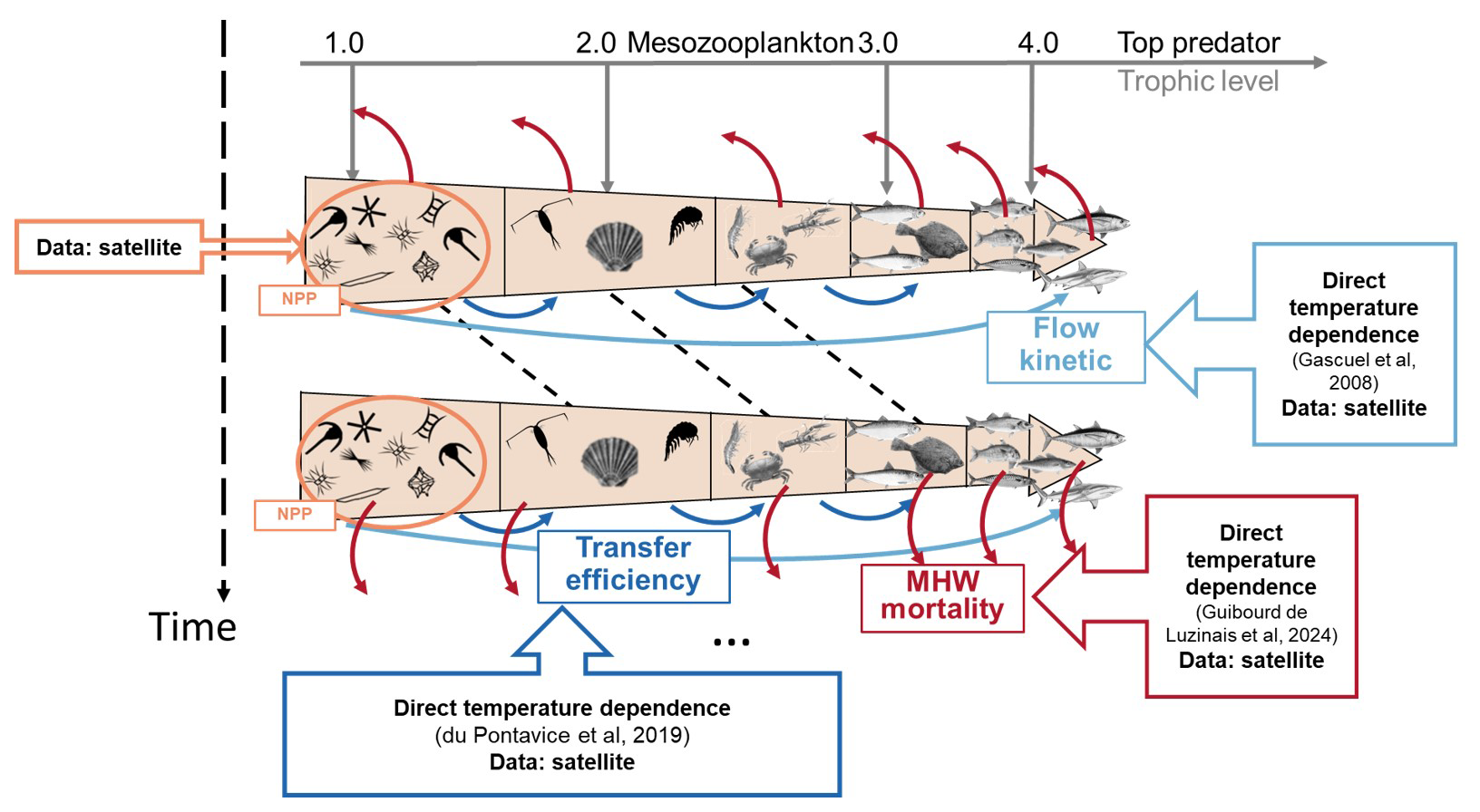
Figure 1 Schematic diagram illustrating the ecological framework represented by EcoTroph-Dyn (adapted from du Pontavice et al., 2021). The trophic functioning of marine food webs is represented by a biomass flow, starting with biomass entering the system at trophic level 1 through net primary production (NPP). Biomass then moves through each trophic level according to trophic transfer efficiency. The flow kinetics, temperature and MHW dependance is crucial in defining trophic class boundaries and estimating biomass for each trophic level over time. When MHWs occur, there is a loss of biomass flow at each trophic level. The empirical models used for each parameter (MHW losses (η), transfer efficiency (TE) and flow kinetic (K)) and where satellite data (SST and NPP) are incorporated into the model to account for marine heatwaves are noted in the figure.

2.2 MHW loss rate algorithm

We compute the loss rate in the biomass flow associated with MHWs based on the percentage of species undergoing thermal stress, i.e. species exposed to temperatures exceeding their thresholds. A detailed description of the MHW loss rate algorithm is described in Appendix A1. Here, we provide the main steps for the incorporation of the effects of marine heatwaves into EcoTroph-Dyn:

1. Detection and characterisation of MHWs with climatology (period of 1982–2011),

2. Estimation of species distribution and associated thermal niche,

3. Matching historical MHW distributions and characteristics with species distribution,

4. Calculation of the percentage of species undergoing thermal stress in each ocean spatial cell,

5. Based on this percentage, estimation of an additional loss rate associated with MHWs.

Finally, we assumed in the mathematical expression of loss rate (η_i) that species are continuously challenged by increased MHW intensity, which is expressed as

$$\begin{array}{}\text{(8)}& {\mathit{\eta }}_i=e^{-e^{b\mathit{\_}t{l}_i\cdot \mathit{\alpha }\cdot \left({\mathrm{MHW}}_{\mathrm{cat},i}-\frac{\mathrm{lt}\mathrm{50}\mathit{\_}t{l}_i}{\mathit{\alpha }}\right)}}\cdot \mathit{\beta },\end{array}$$

where b_tl_i and lt₅₀_tl_i correspond to the slope of the function and the index of marine heatwave intensity (MHW_cat,i) at which 50 % of the species undergo thermal stress in cell_i. β corresponds to the MHW duration, with β ranging from β=0 (no MHW) to β=1 (MHW lasting 15 d) (see Sect. 3.3.1). MHW_cat,i corresponds to an MHW intensity index (defined in Appendix A1), and α is a coefficient assumed to represent the species' resistance capacity to MHW conditions, thus reducing the mortality rate due to species' exposure to thermal stress.

We used an α=0.2 in our simulations. However, we also explored the sensitivity of the results to community resistance capacity by testing four alternative values of α. The α values that we tested were full resistance (α=0, i.e. we fixed η_i=0; no mortality due to thermal stress), partial resistance (α=0.2, 0.5; 20 % and 50 % of the species die because of thermal stress, respectively) and no resistance (α=1; all species die when they are under thermal stress). We performed a three-way ANOVA; that is, a statistical test we used to analyse the effects of trophic levels, biomes and α value on biomass change. We also related the loss rate to the MHW duration over the 15 d by assuming that the duration increased the mortality rate.

2.3 EcoTroph-Dyn simulations

The EcoTroph-Dyn model was applied to simulate consumer biomass and production (between TLs 2 and 5.5) from 1998 to 2021 for each 1° × 1° spatial cell of the global ocean (Fig. S1 in the Supplement). Model outputs were summarised spatially by biome: the tropical, temperate or upwelling biome, based on Reygondeau et al. (2013). We excluded polar biomes because net primary production (NPP) data, one of the forcing variables of the EcoTroph-Dyn model, were not available in high-latitude regions during the winter period.

2.3.1 Environmental forcing data

We simulated and compared consumer biomass and production under scenarios with and without MHWs. The simulations were driven by daily SST observations from the data of the National Oceanic and Atmospheric Administration Advanced Very High Resolution Radiometer (NOAA-AVHRR) (https://www.ncei.noaa.gov/access/metadata/landing-page/bin/iso?id=gov.noaa.ncdc:C00680, DOC/NOAA/NESDIS/NCDC, 2008), as well as NPP data predicted from the EPPLEY-VGPM algorithm and satellite remote sensing data (http://orca.science.oregonstate.edu/npp_products.php, last access: 5 May 2022).

From the daily SST time series in each ocean cell, we identified every MHW day. We defined an MHW as when the daily SSTs exceed an extreme temperature threshold value for at least 5 consecutive days (Hobday et al., 2016). The extreme temperature threshold value was calculated for each 1° latitude × 1° longitude spatial cell as the 90th percentile of daily SST from the 30-year historical time series from January 1982 to December 2011. We did not calculate threshold values by season; thus, MHW events were identified by a single threshold across the year. As a result, we detected MHWs mostly occurring during the year's warmest months. We used the R package heatwaveR described at https://robwschlegel.github.io/heatwaveR/ (last access: 17 October 2022) (Schlegel and Smit, 2018) to detect MHWs in each spatial cell from January 1998 to December 2021.

For the scenarios with MHWs, we used the SST time series from the NOAA-AVHRR data.

To simulate scenarios without MHW in the SST time series, we decomposed the daily SST time series (Y_t) of each ocean spatial cell using a Census X-11 procedure (Pezzulli et al., 2005; Shiskin, 1967; Vantrepotte and Mélin, 2011). With this method, the time series can be decomposed as

$$Y_t=T_t+S_t+H_t,$$

where Y_t represents the daily SST at day t, T_t represents the long-term mean annual changes in temperature, S_t represents the seasonal component (repetitive pattern over time) and H_t represents the additional temperature variability that is not attributed to the annual trend or seasonality.

The T_t underlying long-term direction is obtained from the 365 d running average of the initial series Y_t. The seasonal component (S_t) is then computed by applying a centred moving average to the trend-adjusted series (Y_t−T_t). The estimation of S_t on the trend-adjusted series avoids any confusion with the inter-annual (trend) signal. After the revised estimation of these two components (see the method in Pezzulli et al., 2005; Vantrepotte and Mélin, 2011), the additional temperature variability component was computed as $H_t=Y_t-S_t-T_t$.

We applied the following procedure to create a daily SST time series for the scenarios without MHW. When the daily Y_t value was identified as MHW and Y_t was above the value (T_t+S_t), we replaced the daily SST value (Y_t) with the expected temperature without the additional variability (H_t) component, i.e. T_t+S_t. For MHW days with Y_t below T_t+S_t or non-MHW days, we kept the daily SST value Y_t (see Fig. S2, where the process of creating this time series is illustrated). In our study, we can have an MHW day declared even though $Y_t<T_t+S_t$. This specific situation is rare (less than 0.5 % of time series) and occurs because of the use of an annual threshold value to detect MHW events that mainly occurred during the year's warmest months. (See Fig. S2 just before the month of April for schematic visualisation.) The time series created using this algorithm is referred to here as “without MHW”.

Finally, to adapt the daily SST time series to EcoTroph-Dyn time step resolution ($\mathrm{1}/\mathrm{24}$ year), we aggregated the initial temperature time series Y_t and the “without MHW” time series at a 15 d scale. Specifically, we averaged the daily SST for every 15 d of a year. We then computed the proportion of MHW days (β) within each 15 d. Thus, β=0 when no MHW day is identified in a 15 d time step, and β=1 when an MHW lasts the 15 d of the time step.

Gridded monthly NPP data from 1998 to 2021 were obtained from satellite-derived estimation. The NPP data were estimated using the EPPLEY Vertically Generalized Production Model (VGPM) computation method (Behrenfeld and Falkowski, 1997). The EPPLEY-VGPM method is a hybrid model that employs the basic model structure and parameterisation of the standard VGPM computation. This model estimates net primary production (NPP) based on chlorophyll concentration, incorporating the vertical distribution of primary production. The specificity of the EPPLEY-VGPM method is that the polynomial description of the maximum daily net primary production found in a given water column (Pb_opt, expressed in units of mg of carbon fixed per mg of chlorophyll per hour) is replaced by the exponential relationship described by Morel (1991), based on the curvature of the temperature-dependent growth function described by Eppley (1972).

After excluding spatial cells from the polar biome, we had a total of 34 643 cells, 13 340 of which contained incomplete time series of NPP. For cells with incomplete time series, we utilised the spline function from the R package “stats” to interpolate the missing NPP values. In each ocean cell, the interpolation was constrained by the minimum and maximum satellite data values of the NPP observed over their respective time series. This approach ensured reliable interpolation and reduced potential bias.

Finally, to match the NPP time series with the resolution of the EcoTroph-Dyn time step ($\mathrm{1}/\mathrm{24}$ of a year), we duplicated the monthly NPP values to cover the two sets of 15 d of each month.

2.3.2 Biomass simulations

We simulated the changes in biomass spectra in each spatial cell from 1998 to 2021 for the scenarios with and without MHW. We calculated the differences in consumer biomass change between scenarios with and without MHW. Biomass change was computed using the reference period from 1998 to 2009 under the “without MHW” scenario, allowing us to examine the projected declines in biomass specifically attributable to MHWs. We explored the sensitivity of the results to species' resistance capacity to MHW conditions using the four resistance capacity settings represented by the values of the coefficient α.

We initialised the model by applying a “burn-in” period of 12 years without any environmental forcing. Indeed, simulation testing indicates that a burn-in period of at least 10 years is needed for biomass spectra to reach equilibrium (Fig. S3). Increasing the burn-in period beyond 12 years does not significantly change the equilibrium biomass spectra (t test p value = 0.6118). We thus used the average of the time series (1998 to 2021) as the burn-in period in each ocean spatial cell.

2.3.3 Northeastern Pacific Ocean MHW case study

An analysis focusing on the MHW that occurred in the northeastern Pacific Ocean from 2013 to 2016 (commonly known as “the Blob”; Bond et al., 2015) was undertaken to assess the capability of EcoTroph-Dyn to transcribe past MHW events. First, we extracted the EcoTroph-Dyn simulation outputs (with and without MHW) in the region, delineated by the boundary of nine biogeochemical provinces that had been identified by Reygondeau et al. (2013) and adapted from Longhurst (2007). These biogeochemical provinces include the Central American coast (CAMR), California ocean and California coastal current (OCAL and CCAL), Alaska coastal downwelling (ALSK), North Pacific tropical gyre (NPTG), northeastern Pacific subtropical (NPSE), North Pacific polar front (NPPF), Eastern Pacific subarctic gyres (PSAE) and Western Pacific subarctic gyres (PSAW). Second, we computed biomass change using the reference period from 1998 to 2009 under the “without MHW” scenario, allowing us to examine the projected declines in biomass specifically attributable to the Blob. Finally, we discussed and compared our results with the literature.

3 Results

3.1 Environmental forcing with and without MHWs

In response to climate change, the NPP and SST are already perturbed. Global total NPP decreased by 1 % in the period 2015–2021 compared to the 1998–2009 period. However, large spatial variability was observed in NPP changes (Fig. 2a). In particular, NPP decreased by 20 % in the northeastern Pacific, while an increase of 20 % was estimated for the Southern Ocean. Under the “without MHW” scenario (Fig. 2b), global average SST increased by 0.28 °C in the period 2015–2021 compared to the 1998–2009 period, with some areas warming by up to 0.5 °C. However, under the “with MHW” scenario (Fig. 2c), SST increased by 0.32 °C in 2015–2021 compared to the period 1998–2009, with some areas, such as the northeastern Pacific, warming by up to 1 °C over the same period. Globally, the estimated increase in average SST from 2015 to 2021 was 4 % higher in the “with MHWs” scenario compared to the “without MHW” scenario.

Under the “with MHWs” scenario, MHWs occurring during the year's warmest month increased in intensity, duration and surface extent from 1998 to 2021 (Fig. 3a, b), with large spatial variability (Fig. 3c, d). MHWs with intensity lower than 3 °C above the climatology were identified on average in 28.5 % of the ocean surface (Fig. 3a). These MHWs lasted, on average, more than 40 d (Fig. 3b). In contrast, MHWs characterised as higher intensity (≥ 3 °C above climatology) were identified in < 20 % of the ocean surface area (Fig. 3a). These relatively more intensive MHWs lasted, on average, 32 d (Fig. 3b). Furthermore, more MHW days of lower intensity were identified for low-latitude regions (23° N–6° S) (Fig. 3c, d) compared to MHW days identified in higher latitude regions (> 23° N and 25° S).

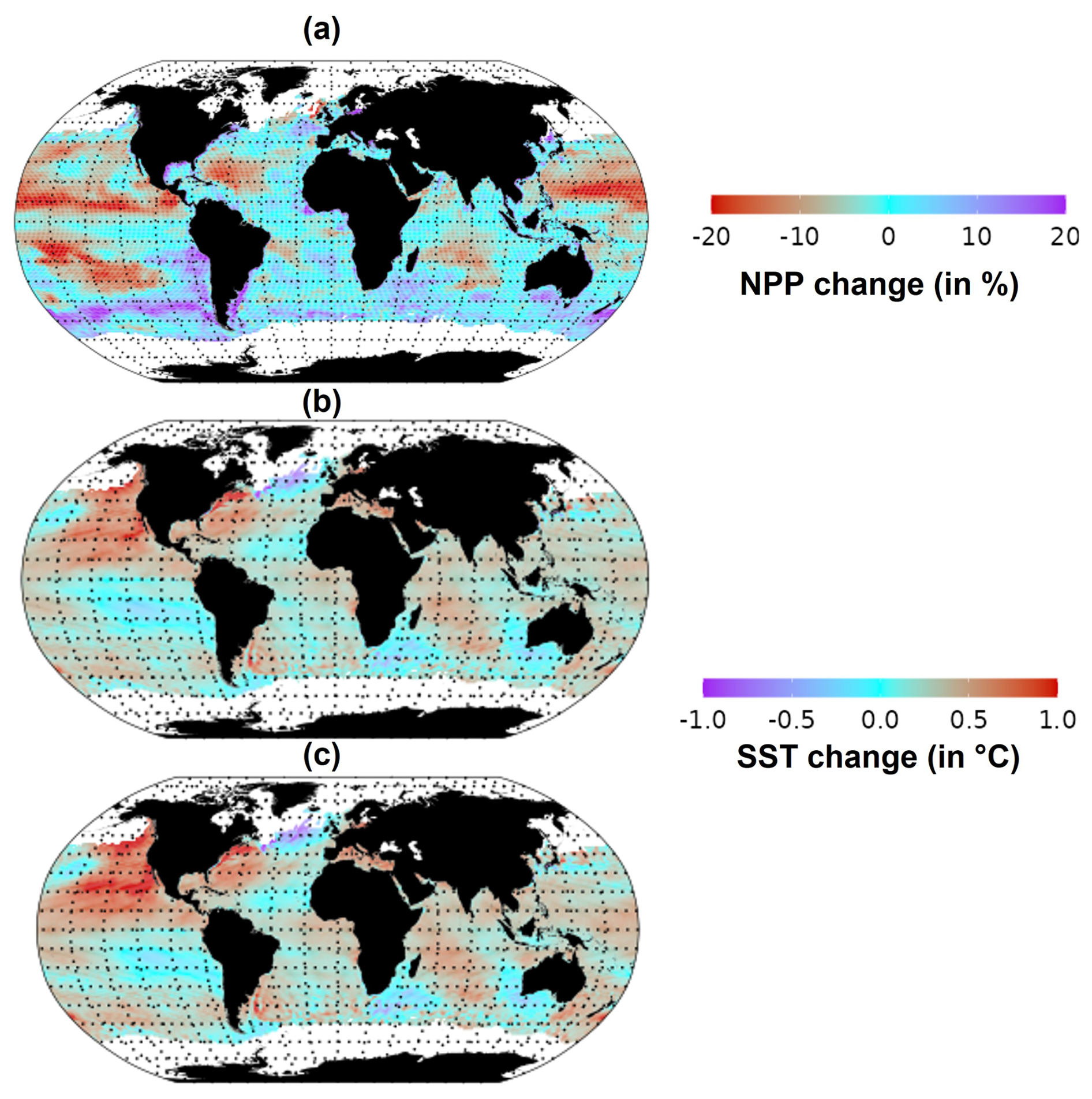
Figure 2 Changes in SST and NPP between the average of 2015–2021 relative to the average of 1998–2009. (a) NPP, (b) SST under the “without MHW” scenario and (c) SST under the “with MHWs” scenario.

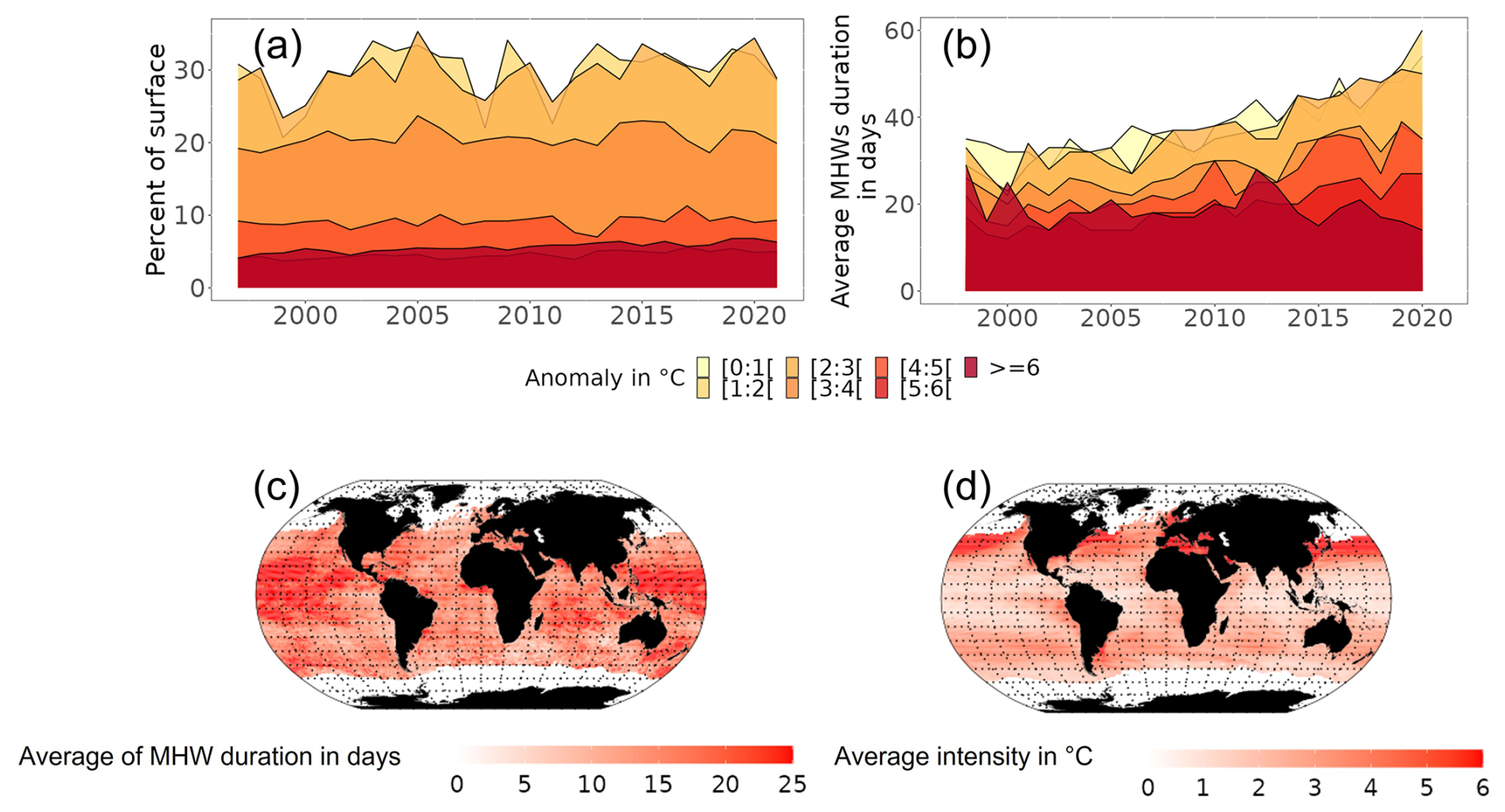
Figure 3 Temporal and spatial characteristics of MHWs identified for the period 1998 to 2021. (a) Changes in the percentage of the oceans' total surface area with MHW in each year categorised by their intensity. (b) Evolution of average duration of MHWs categorised by their intensity. (c) Average duration of each MHW event in days that occurred over the period 2015–2021. (d) Average intensity of each MHW event over the period 2015–2021.

3.2 Biological impacts of MHWs at the global scale

3.2.1 Impact on total consumer biomass

The projected changes in total consumer biomass were higher under the “with MHWs” scenario relative to the “without MHW” scenario. Globally, total consumer biomass was projected to decrease on average by 0.07 ± 0.02 % yr⁻¹ (standard error) relative to the baseline period of 1998–2009 (Fig. 4a) (GLS, generalized least squares, p value < 0.05). In contrast, simulations under the “with MHWs” scenario with an MHW resistance capacity setting of α=0.2 projected an average decrease in total consumer biomass of 0.12 ± 0.02 % yr⁻¹ relative to the baseline period of 1998–2009 (p value < 0.05). Thus, simulations that focussed on annual mean changes in temperature only masked the effects of MHWs on the long-term changes in consumer biomass in the ecosystem (Fig. S4).

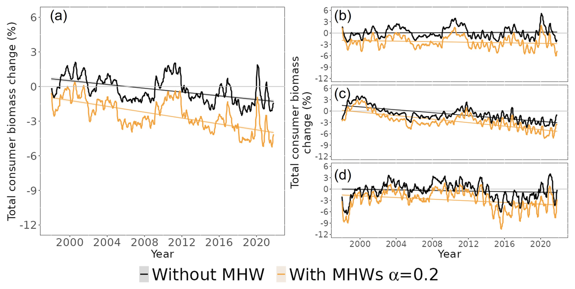
Figure 4 Simulated total consumer biomass change in the ocean from 1998 to 2021 under the “without MHW” (black lines) and “with MHWs” (light-orange lines) scenarios, with a resistance capacity setting of α=0.2: (a) the world ocean (excluding the polar biome), (b) temperate biomes, (c) tropical biomes and (d) upwelling biomes, respectively (Fig. S1 for biome spatial definition). The horizontal grey line separates the positive and negative total consumer biomass changes.

While total consumer biomass was projected to decrease slightly across the three biomes (temperate, tropical and upwelling biomes represented in Fig. 4b, c and d, respectively), in the scenario “with MHWs”, the declines in tropical biomes were larger than the global average. Under the “without MHW” scenario, total consumer biomass in temperate biomes was projected to increase by 0.01 % ± 0.01 (standard error), while in tropical and upwelling biomes, it was projected to decrease by 0.18 % ± 0.01 and 0.02 % ± 0.01 yr⁻¹, respectively, relative to the baseline period. Under the “with MHWs” scenario with α=0.2, total consumer biomass in temperate, tropical and upwelling biomes was projected to decrease more strongly by 0.03 % ± 0.01 %, 0.23 % ± 0.02 % and 0.10 % ± 0.02, respectively, relative to the baseline.

3.2.2 Impacts by trophic level

MHWs exacerbated the projected climate change impacts on biomass, particularly for higher trophic-level groups. Indeed, our model projected a similar level of biomass loss across trophic levels in the “without MHW” scenario, with a projected decrease in global total consumer biomass of 1.0 ± 0.1 % SE in the period 2015–2021 relative to 1998–2009 (Fig. 5a–c – black lines). In contrast, under the “with MHWs” scenario and with a resistance capacity setting of α=0.2, total consumer biomass was projected to decrease by 4.4 ± 0.1 % for high trophic-level classes (TL ∈ [4;5.5]), while the decrease was smaller for the low trophic-level (TL ∈ [2;3[, 3.4 ± 0.1 %) and mid-trophic-level (TL ∈ [3;4[, 4.1 ± 0.1 %) classes (Fig. 5a–c – light-orange lines).

The impact on high trophic levels differed between biomes, with the tropical and upwelling biomes being notably more impacted. Under the “without MHW” scenario, our model projected a decrease in high trophic-level consumer biomass of 0.5 ± 0.1 % SE, 2.4 ± 0.1 % and 2.2 ± 0.1 % in temperate, tropical and upwelling biomes, respectively, in the period 2015–2021 relative to 1998–2009 (Fig. 5f, i and m – black lines). In contrast, under the “with MHWs” scenario and with a resistance capacity setting of α=0.2, high trophic-level consumer biomass was projected to decrease by 3.3 ± 0.1 %, 6.6 ± 0.1 % and 5.9 ± 0.1 % in temperate, tropical and upwelling biomes, respectively, while a smaller biomass decrease for the low and mid-trophic level was expected (Fig. 5f, i and m – light-orange lines).

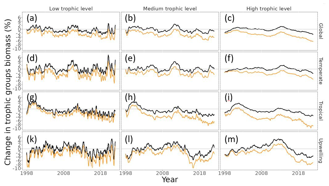
Figure 5 Projected changes in consumer biomass for each trophic level and biome relative to the 1998–2009 average under the “without MHW” (black lines) and “with MHWs” (light-orange lines) scenarios, with low trophic level (TL ∈ [2;3[), medium TL (TL ∈ [3;4[) and high TL (TL ∈ [4;5.5]). Panels (a)–(c) correspond to the global scale; panels (d)–(f) correspond to the temperate biome; panels (g)–(i) correspond to the tropical biome; and panels (k)–(m) correspond to the upwelling biomes. Panels (a), (d), (g) and (l) correspond to low TLs; panels (b), (e), (h) and (l) correspond to medium TLs; and panels (c), (f), (i) and (m) correspond to high TLs. The simulation results under the “with MHWs” scenario used a resistance capacity setting of α=0.2.

3.2.3 Various responses of ecosystems to MHWs

Over the 2015 to 2021 period, MHWs impacted total consumer biomass with large variations in both the direction and magnitude of the impacts between biomes (Fig. 6). Under the “without MHW” scenario, the model projected an increase in total consumer biomass in 33.5 % of the ocean area, especially in temperate biomes (Fig. 6a). Under the “with MHWs” scenario, this proportion decreased, and a biomass increase was projected to occur in only 24 % of the global ocean, with a projected global biomass decrease of 4.8 % in the period 2015–2021 relative to 1998–2009 (compared to only a 2.4 % biomass loss under the “without MHW” scenario). In high latitudes (> 25° N and 25° S), MHWs exhibiting high intensity but short duration (Fig. 3c and d) resulted in moderate additional biomass losses, up to 8 % in 2015–2021 (Fig. 6c). Conversely, in low latitudes (25° N–25° S), MHWs led to substantial additional biomass losses, exceeding 10 % on average (Fig. 6c), and up to 20 % in biodiversity hotspots such as Indonesia, off the coast of Papua New Guinea and Central America. Thus, high-latitude and upwelling areas appeared to be refuge zones from MHWs compared to the low latitudes. Looking at the MHW's additional impact in food webs (Figs. S5, S6 and S7), similar spatial patterns and responses are projected with a higher impact (biomass decreases) on high trophic levels compared to lower trophic levels.

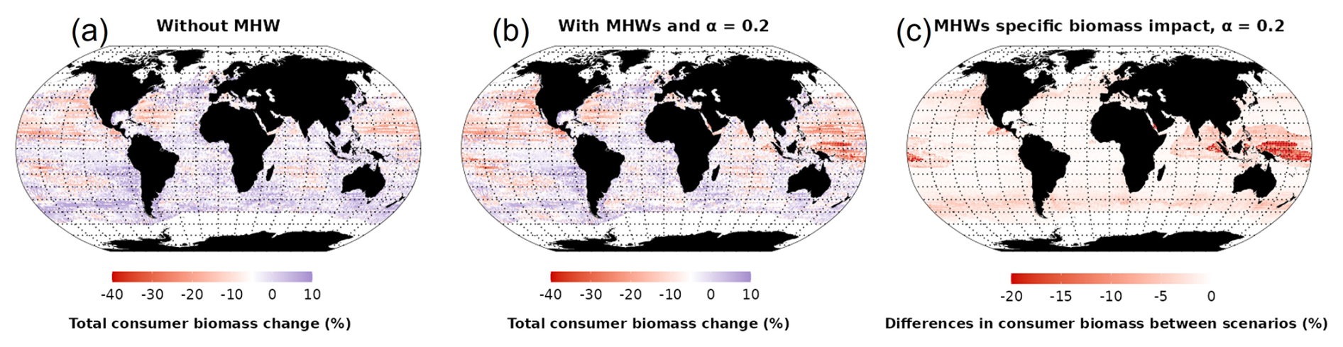
Figure 6 Changes in total consumer biomass during 2015–2021 compared to 1998–2009. (a) Total consumer biomass under the “without MHW” scenario, (b) total consumer biomass under the “with MHWs” scenario with α=0.2 and (c) differences in consumer biomass between scenarios.

3.3 Sensitivity to resistance capacity setting (α)

Ecosystem total consumer biomass response to MHWs depended on community resistance capacity. Assuming species have full resistance (α=0) or no resistance (α=1) to MHWs, total consumer biomass was projected to decrease by 2.3 % and 15.3 % in the period 2015–2021 relative to 1998–2009, respectively (Fig. 7a). Simulations using different α values projected changes in total consumer biomass that were consistent in direction but differed significantly in magnitude. A three-way ANOVA was performed to analyse the effect of trophic levels, biomes and α value on biomass change. This ANOVA revealed a statistically significant effect on biomass change of trophic levels, biomes and α values (p value < $\mathrm{2}\times {\mathrm{10}}^{-\mathrm{16}}$), individually. Additionally, the interaction between biomes, trophic levels and α value had a significant effect on biomass change (F(27, 16 737) = 442.4, p value $<\mathrm{2}\times {\mathrm{10}}^{-\mathrm{16}}$). The lower the resistance capacity of species (higher α value), the greater the loss of total consumer biomass. On a biome scale, these variations in biomass loss were greater for the tropics, with values ranging from 3.1 % (α=0) to 20.2 % (α=1) (Fig. 7c). In comparison, sensitivity was lower in the temperate and upwelling biomes, with a decrease between 1.4 % (α=0) and 11.2 % (α=1) and between 3.8 % (α=0) and 12.3 % (α=1), respectively (Fig. 7b and d).

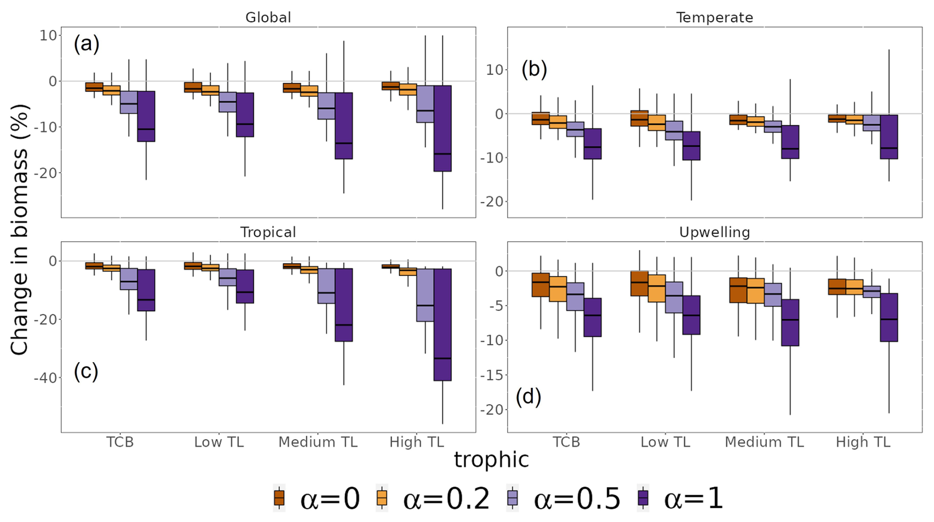
Figure 7 Sensitivity of changes in total consumer biomass to different resistance capacity settings. Changes are aggregated for the whole biomass spectrum (TCB) and by trophic level (TL) (low TL, medium TL and high TL). Colours represent different resistance capacity settings (α values): (a) global ocean, (b) temperate biomes, (c) tropical biomes and (d) upwelling biomes. The different horizontal lines of the box plot refer to the median, 25th and 75th quantiles.

The sensitivity of changes in total consumer biomass to the resistance setting increased with trophic level. At a global scale, the response of low TLs ranged from a consumer biomass decrease of 1.4 % (α=0) to 8.0 % (α=1), while high TLs exhibited values ranging from 0 % (α=0) to 11 % (α=1) (Fig. 7a). Furthermore, the sensitivity of trophic levels to the α value was greater in the tropical biome and lower in the temperate and upwelling biomes relative to that of the global ocean.

3.4 A case study of a northeastern Pacific MHW

Our model projected that the MHW in the northeastern Pacific from 2013 to 2016 (the Blob) resulted in long-term changes in the biomass spectrum in the region (Fig. 8c). Temperature anomalies were on average ≥ 4 °C (between 2013 and 2016) and up to 8 °C in 2015 relative to 1982–2011. This temperature anomaly had some ecological repercussions. On average, without accounting for MHWs, total consumer biomass in our simulation was hindcast to decrease by 1.5 % ± 0.3, 3.1 % ± 0.4, 6.6 % ± 0.2 and 5.2 % ± 0.3 in 2013, 2014, 2015 and 2016, respectively, compared to the reference period of 1998 to 2009 (black line in Fig. 8c). However, when accounting for MHWs with α=0.2, the total consumer biomass loss decreased on average by an additional 3.1 % in 2013, 2014, 2015 and 2016. Furthermore, the difference in linear trend (slope and intercept) between the biomass time series 1998 to 2013 and 2017 to 2021 indicated that the MHW (the Blob) had a significant effect on long-term changes in biomass (GLS, generalized least squares, p value < 0.05).

The magnitude of the hindcast total consumer biomass differed significantly between biogeochemical provinces (ANOVA, F(1, 2906) = 7.854, p value < 0.05, Fig. 8d). Comparing the consumer biomass before (1998–2012) and during (2013–2016) the occurrence of the Blob, all biogeochemical provinces in the northeastern Pacific, except the Alaska coastal downwelling (ALSK) and Central American coast (CAMR), exhibited a significant total consumer biomass decrease (ANOVA, F(1, 151) = 155.443, p value < $\mathrm{2}\times {\mathrm{10}}^{-\mathrm{16}}$) under the scenario with and without MHWs. Under the “without MHW” scenario, total consumer biomass in the North Pacific tropical gyre (NPTG) biogeochemical provinces, followed by the California current (CCAL+OCAL biogeochemical provinces), was hindcast to decline the most amongst the provinces when comparing before, during and after the Blob (Fig. 8d). Under the “with MHWs” scenario and with a resistance capacity setting of α=0.2, all biogeochemical provinces were hindcast to have an additional biomass decrease during and after the Blob. This additional biomass decrease ranged from 0.9 % to 5 % and from 1.4 % to 5.1 % during and after the Blob, with an average decrease of 2.7 % ± 0.4 % and 3.1 % ± 0.3 %, respectively (Fig. 8d). In particular, the California current and the Alaska coastal downwelling provinces were most affected by the MHW, with additional biomass decreases of 5 % and 3.8 % relative to the “without MHW” scenario, during and after the Blob.

The impact of the Blob on various trophic levels was similar to the global pattern, with a rapid reaction (in terms of biomass loss) observed at lower TLs and higher TLs exhibiting a delayed response (Fig. S8). Considering the influence of MHWs from 2013 to 2016 using the “with MHWs” scenario and α=0.2 resistance capacity, there was a hindcast biomass reduction of 6.8 % ± 0.7, 6.3 % ± 0.6 and 4.3 % ± 0.3 for low, medium and high TLs, respectively, when compared to the reference period of 1998 to 2009. Compared to pre-event conditions, by 2021, aside from low TLs, medium and high TLs gave no sign of recovery from the Blob MHW event.

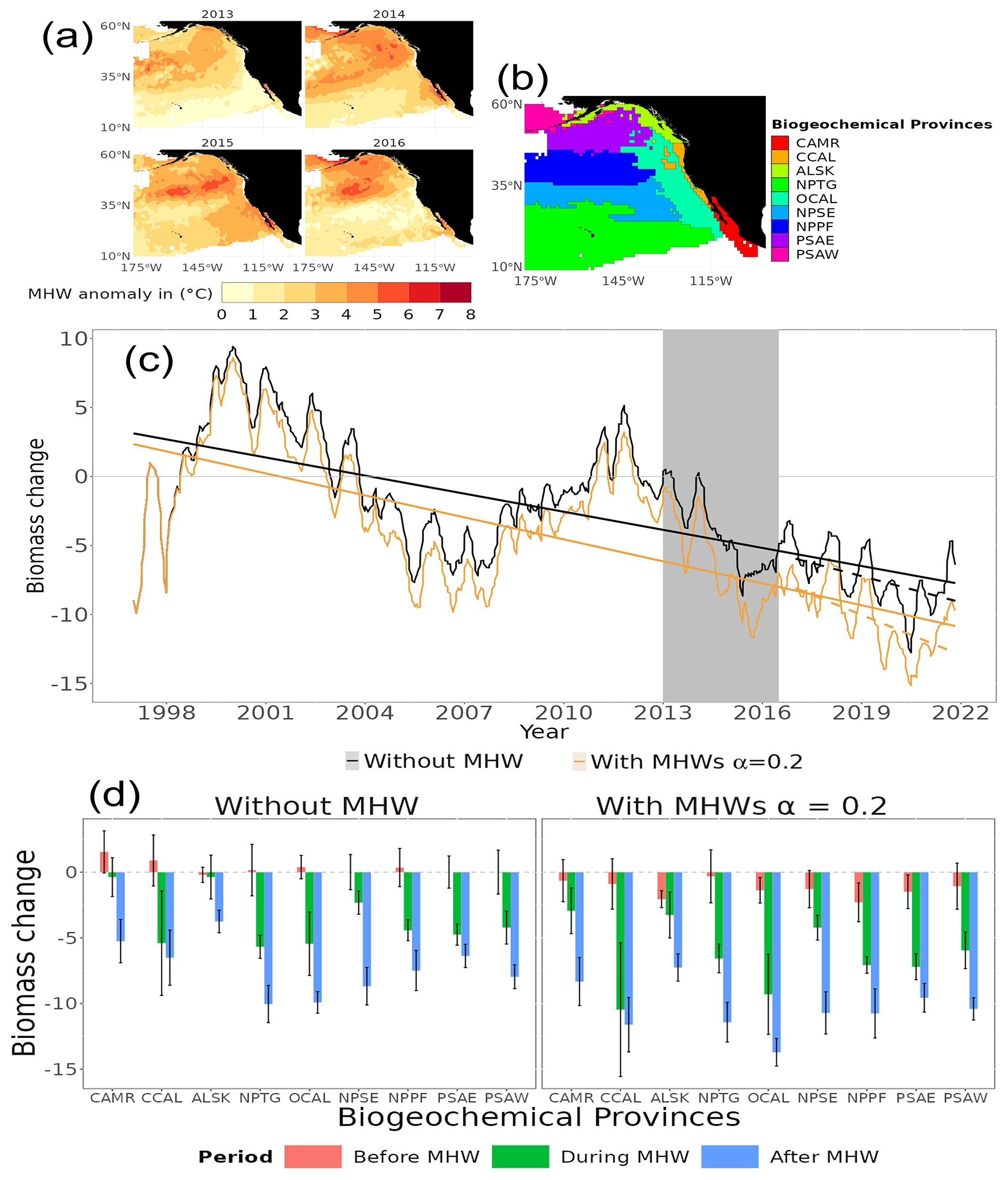
Figure 8 Hindcast of temporal and spatial biological impacts of the MHW from 2013 to 2016 in the northeastern Pacific (the Blob). (a) Temperature anomalies between 2013 and 2016. (b) Biogeochemical provinces definition, with Central American coast (CAMR), California ocean and coastal current (OCAL and CCAL), Alaska coastal downwelling (ALSK), North Pacific tropical gyre (NPTG), northeastern Pacific subtropical (NPSE), North Pacific polar front (NPPF), Eastern Pacific subarctic gyres (PSAE) and Western Pacific subarctic gyres (PSAW). (c) Generalised least squares models (lines) and total consumer biomass change in the “without MHW” and “with MHWs” scenarios in the black and light-orange colours, respectively. The vertical grey shaded area indicates the duration of the Blob. (d) Average total consumer biomass changes before (1998–2012 – pink), during (2013–2016 – green), and after (2017–2021 – blue) the Blob for each biogeochemical province. The error bars correspond to standard errors.

Trophic dynamics of the biomass spectra in the northeastern Pacific were hindcast to be impacted by the Blob (Fig. S9). The trophodynamic indicators flow kinetic and trophic efficiency increased and decreased, respectively, in the model. Under the scenario “without MHW”, the average hindcast flow kinetic of the biomass spectra in the northeastern Pacific increased by 0.6 % ± 0.2, while the transfer efficiency decreased by 0.7 % ± 0.2 in the period 2013–2016 relative to 1998–2009. Consideration of the MHW under the “with MHWs” scenario exacerbated the increase in flow kinetic and decrease in trophic efficiency significantly by 0.7 % and 0.4 %, respectively (t test p value < 0.05).

4 Discussion

In this study, we accounted for MHWs in the last four decades using hindcast simulations and showed the potential of synergistic impacts of MHWs (pulses) and long-term climate change (presses) on biomass and trophodynamics of ecosystems (Bender et al., 1984; Harris et al., 2018). These reconstructed MHW impacts varied spatially because of MHW spatial dynamics, regional differences in ocean biogeochemical and physical conditions and ecosystem trophodynamic characteristics. Furthermore, in studying the Blob, we highlighted the fact that MHWs could exacerbate the long-term impacts of climate change that vary between biogeochemical provinces.

4.1 Impacts of MHWs on global marine consumer biomass

Over the past two decades, MHWs have led to increased mortality rates and significant alterations in the functioning and structure of ecosystems (Smith et al., 2023; Wernberg et al., 2013, 2016). Our modelling analysis suggests that, without accounting for MHWs and their ecological effects, the decline in global-scale biomass associated with climate change may have been significantly underestimated. We show that MHWs have exacerbated the impacts of long-term climate change, impacting trophodynamic parameters such as the flow kinetic and transfer efficiency in ecosystems, which is congruent with studies by Arimitsu et al. (2021), Gomes et al. (2024) and Smith et al. (2023). These perturbations in ecosystem functioning result in biomass loss through food webs. Although MHW temperature anomalies have mostly lasted for weeks to months only, we emphasise that the resulting ecosystem perturbations last for a longer time (decades) and influence long-term biomass change (Fig. 8; Babcock et al., 2019; Cheung and Frölicher, 2020; Guibourd de Luzinais et al., 2024). Finally, the intensity and duration of MHWs have influenced the magnitude of the perturbation in ecosystem functioning (Oliver et al., 2021; Smith et al., 2023). We have highlighted the fact that the intensity and duration of MHWs have continuously increased since the beginning of the 21st century (Fig. 3), leading to a sharp biomass decrease over the hindcast period (Fig. 4). Such short-term biomass decreases have strengthened the impacts of long-term climate change (Cheung and Frölicher, 2020; Collins et al., 2019).

At a global scale, over the whole time series and in different MHW resistance capacity scenarios, high TL biomass experienced greater impacts from MHWs and was not able to recover to pre-perturbation levels as effectively as the low and medium TL biomass. The gap in biomass recovery was most apparent in tropical and upwelling biomes, where the hindcast biomass of high TLs consistently decreased over time. The time needed for the biomass to return to pre-perturbed levels was related to the rate of biomass turnover, which was also dependent on the speed of biomass flows. This turnover decreased with trophic level and was low for organisms at the top of the food chain (Gascuel et al., 2008; du Pontavice et al., 2020; Schoener, 1983). Thus, the high frequency of MHWs in recent years may be greater than the time that high TLs need to recover from the impacts of individual MHWs; this could contribute to the continued decline in high-TL biomass.

4.2 Trophodynamics approach as a framework for deciphering ecosystem responses to MHWs

In our modelling approach, trophodynamic changes were assessed through transfer efficiency (TE) and flow kinetics. TE (dimensionless) is defined as the fraction of energy transferred from one trophic level (TL) to the next and summarises all the losses in the trophic network (Jennings et al., 2002; Libralato et al., 2008; Lindeman, 1942; Niquil et al., 2014; Pauly and Christensen, 1995; Schramski et al., 2015; Stock et al., 2017). It is an emergent property of marine ecosystems and an essential parameter in many applications of marine ecology, such as estimating biomass flux in production models (e.g. Carozza et al., 2016; du Pontavice et al., 2021; Gascuel et al., 2011; Jennings et al., 2008; Tremblay-Boyer et al., 2011). Unlike previous applications of EcoTroph at an annual timescale (du Pontavice et al., 2021, 2023), where changes in transfer efficiency reflected long-term changes in species assemblages, having a transfer efficiency that evolved on a biweekly basis (14 d) allowed us to take into account metabolic fluctuations over a shorter period. The temperature during MHWs increases the basal metabolism (catabolism) of marine organisms (Grimmelpont et al., 2023; Minuti et al., 2021), thus reducing the energy available for anabolic processes that can only occur once catabolic needs are met (Eddy et al., 2021). The estimation of transfer efficiency only considers anabolic processes (Eddy et al., 2021); hence, this balance between catabolism and anabolism is how MHWs could disrupt transfer efficiency on a biweekly scale. The flow kinetics expressed in TL yr⁻¹ quantifies the speed of the trophic flux, i.e. the rate of biomass transfer from lower trophic levels to higher ones, due to predation and/or ontogenesis (Gascuel et al., 2008; du Pontavice et al., 2020). This rate is inversely proportional to the biomass residence time (BRT; du Pontavice et al., 2020), which is the average time a unit of biomass spends moving from one TL to the next higher one through predation (Gascuel et al., 2008; Schramski et al., 2015). This flow kinetics can be measured by the production $/$ biomass ratio (P $/$ B; Gascuel et al., 2008), which is used in many ecosystem models, particularly Ecopath with Ecosim (EwE; Christensen and Pauly, 1992).

MHWs disrupt the metabolism of individuals and, on a larger scale, impact the entire ecosystem with trophodynamic changes throughout the trophic network (Fig. S9; Arimitsu et al., 2021; Collins et al., 2019; Gomes et al., 2024; Smith et al., 2023). However, due to their different physical characteristics depending on the ecosystems and the varying functioning of these ecosystems, they do not induce the same structural and functional changes, leading to different biomass losses. Tropical ecosystems are composed of species with low transfer efficiency (TE, low ratio between stored energy and ingested energy), with significant energy losses that increase with temperature (Brown et al., 2004; du Pontavice et al., 2020; Schramski et al., 2015). To compensate for this low efficiency, predation activity is high, resulting in rapid biomass transfers between prey and predators (biomass flow; du Pontavice et al., 2020). In these ecosystems, communities (which may be dominated by short-lived and fast-growing species) are generally living at the upper end of their thermal preferences (Begon and Townsend, 2021; Pinsky et al., 2019; Vinagre et al., 2016). They experience thermal stress associated with MHWs, leading to substantial mortality across the trophic network, with a higher proportion occurring in lower trophic levels regardless of the intensity of the MHWs as low TLs tend to have lower thermal limits than high TLs (Guibourd de Luzinais et al., 2024). MHWs scarcely affect transfer efficiency (TE), with an estimated average decrease of 0.05 % between 1998 and 2021 because the metabolism of species is already very high (du Pontavice et al., 2020). However, MHWs exacerbate prey mortality rates, resulting in proportionally higher predation rates, i.e. biomass remains for a shorter time at each trophic level, corresponding to an acceleration of biomass flow (estimated at 1 % on average between 1998 and 2021). Given the relatively high number of MHW days (Fig. 3; Hobday et al., 2018; Marin et al., 2021; Oliver et al., 2018), these modifications to biomass flow are “persistent” and involve significant biomass losses.

In temperate ecosystems, biomass is transferred more slowly between trophic levels, with less loss (higher trophic efficiency; du Pontavice et al., 2020; Eddy et al., 2021). In EcoTroph-Dyn, temperate communities experience thermal stress and mortality only during high-intensity MHWs (Guibourd de Luzinais et al., 2024). MHWs affect the metabolic efficiency of species by increasing basal metabolism and respiration-related losses, which decreases TE across the trophic spectrum, estimated in our simulations at an average of 0.2 % between 1998 and 2021. These higher metabolic demands lead to an increase in predation activity, which, combined with lower mortality (compared to tropical waters), reduces the biomass residence time at each trophic level in the food chain, i.e. a slight acceleration of the speed of biomass flow between each trophic level (estimated in our simulations at an average of 0.3 % between 1998 and 2021). Since MHWs in these ecosystems are characterised by significant temperature anomalies but over relatively short durations (Fig. 3; Frölicher et al., 2018; Oliver et al., 2018), these modifications to biomass flow are “temporary” and involve lower biomass losses.

Finally, in upwelling ecosystems, communities are characterised by low transfer efficiencies with high biomass residence times, indicating slow biomass transfers between prey and predators (du Pontavice et al., 2020). MHWs cause thermal stress and moderate mortality in these ecosystems (Guibourd de Luzinais et al., 2024). They lead to a decrease in the metabolic efficiency of species (estimated in our simulations at an average of 0.03 % between 1998 and 2021), along with an increase in predation activity, moderately impacting the rate of biomass flows in the ecosystem (estimated in our simulations at an average of 0.3 % between 1998 and 2021). The MHWs occurring in these ecosystems are of high intensity and last relatively long (an average of 23 d yr⁻¹ between 1998 and 2021). One might expect more significant impacts than in tropical environments; however, this was not the case. This could potentially be explained by (i) the high productivity of these ecosystems, which supports a highly biodiverse food web (Largier, 2020; Pauly and Christensen, 1995; Rykaczewski and Checkley, 2008; Ryther, 1969), leading to better resilience to environmental changes and extreme temperature events (Bernhardt and Leslie, 2013); and (ii) the specific functioning of these ecosystems with cool water rising from depth to the surface, which tends to reduce the number of MHW days compared to the adjacent open ocean (Varela et al., 2021). More generally, it has been highlighted that ocean warming does not affect coastal regions with upwelling in the same way as the open ocean (Varela et al., 2021).

Generally, in our simulations, higher temperatures and frequent mortality events promoted the emergence of species and the growth of populations, adapted to warm waters, both characterised by rapid growth and short lifespans (Beukhof et al., 2019; du Pontavice et al., 2020). This phenomenon was observed, for example, during the Blob event in the California ocean and California coastal current (OCAL and CCAL) provinces, with an increase of tropical species that usually live much farther south, such as tuna, sailfish and marlin (Cavole et al., 2016).

The specific examination of the Blob allowed us to elucidate how this MHW differentially affected the biogeochemical provinces (Longhurst, 2007; Reygondeau et al., 2013) and influenced their long-term responses. According to our simulations (Fig. 8), the biomass in the affected oceanic regions had not returned to the reference levels (1998–2009) by 2021. Following the MHW, all biogeochemical regions experienced significant biomass losses (ANOVA, p value < 0.05), although with varying magnitudes. Differences in exposure to the intensity and duration of temperature anomalies can potentially explain these differences in responses. For example, the coastal part of the California current and the subarctic gyres of the northeastern Pacific were subject to lower anomalies of different durations (Varela et al., 2021). In addition, differences in the structure and functioning of trophic networks may also have contributed to the variation in responses to MHWs between provinces (Morgan et al., 2019; Peterson et al., 2017; Ruzicka et al., 2012). The biogeochemical zones have different compositions of pelagic communities that may respond differently to MHWs (Peterson et al., 2017). For instance, the Gulf of Alaska saw its planktonic community shift towards smaller plankton and zooplankton, resulting in a loss in the nutritional quality and quantity of the forage portion of the pelagic community for their predators, highlighting the disruption of biomass flow (Arimitsu et al., 2021; Piatt et al., 2020; Suryan et al., 2021). In contrast, in the California current biogeochemical region, the MHW was associated with a substantial increase in the abundance of pyrosomes, which implied a limitation of energy flow moving towards higher trophic levels (Gomes et al., 2024). This was not necessarily the case for the oceanic part of the California current. These different changes in the composition and abundance of the lower trophic levels are represented in EcoTroph-Dyn by changes in the amount of energy flowing through the food web. EcoTroph-Dyn also takes into account the differences in trophodynamic characteristics (e.g. transfer efficiency, flow kinetics) between biogeochemical zones. For example, communities in the Gulf of Alaska are more efficient than those in the Californian current (du Pontavice et al., 2020), and the energy entering the food web was less disrupted than in the California current, which may explain the greater impact of the MHW on the California current.

4.3 Model validation and sources of uncertainties

We have developed an innovative approach to modelling marine ecosystems, linking trophic ecology with MHW hindcast to assess their ecological impacts on a seasonal timescale and at a global scale. Despite its apparent simplicity and the reduced number of parameters, EcoTroph-Dyn is part of the family of “complete ecosystem models and dynamic system models” (Plagányi, 2007) as it represents all trophic levels, from primary producers to top predators. It merges individual “species” into categories defined solely by their trophic level and describes ecosystems through a continuous distribution of biomass (trophic biomass spectrum), from primary producers to top predators. EcoTroph-Dyn does not account for specific climate effects on individual species and populations. The model assumes that variations in environmental conditions will lead to new biomass transfer dynamics in theoretical ecosystems at equilibrium. EcoTroph-Dyn meets the criteria described by Link (2010) to be considered a plausible representation of marine ecosystems. These criteria include the following: (i) the biomass values of all functional groups must cover 5 to 7 orders of magnitude, (ii) there must be a 5 % to 10 % decrease in biomass density (on a logarithmic scale) for each unit increase in trophic level, (iii) specific biomass production values (P $/$ B) must never exceed specific biomass consumption values (C $/$ B) and (iv) the ecotrophic efficiency (EE) for each group must be less than 1. Additionally, the model relies on empirically obtained equations (Gascuel et al., 2008; du Pontavice et al., 2020) and has demonstrated its ability to replicate the effects of fishing and climate change on marine ecosystems (e.g. du Pontavice et al., 2021, 2023; Tremblay-Boyer et al., 2011).

To discuss the validity of our hindcasts, we focussed on the most studied MHW (the Blob) in the literature with available quantitative data (e.g. Arimitsu et al., 2021; Bond et al., 2015; Cavole et al., 2016; Cheung and Frölicher, 2020; Gomes et al., 2024; Piatt et al., 2020; Suryan et al., 2021). The historical biomass change simulations from our “with MHWs” simulations and the α=0.2 scenarios showed the same biomass evolution per trophic group as the observational data based on species biomass surveys (Suryan et al., 2021). However, our historical simulations estimated lower biomass and also showed a smaller biomass decrease compared to observed data (Suryan et al., 2021). This would indicate a possible underestimation of biomass and ecosystem response to MHWs by EcoTroph-Dyn. The underestimation of ecological responses to MHWs is likely caused by the choice of a lower α value that lowers the sensitivity of the ecosystem to MHWs. To reduce the uncertainty over the α value, future studies could calibrate it for specific regions using observational data of MHW impacts on marine ecosystems' biomass.

Our simulations of biomass changes, according to the “with MHWs” and α=0.2 scenarios, also fell within the range of historical biomass simulations reported by studies using other approaches to represent ecosystem functioning (e.g. the species-based Dynamic Bioclimate Envelope Model (DBEM) by Cheung and Frölicher (2020) and Ecotran, an extension of the popular Ecopath modelling framework by Gomes et al. (2024); see Fig. 9). Additionally, we projected that the trophodynamic kinetic parameter of biomass flow increased by 3 % in the “with MHWs” and α=0.2 scenarios, which is consistent with the estimates highlighted by Gomes et al. (2024) (3.7 %). Finally, the decreases in trophodynamic transfer efficiency parameters highlighted in EcoTroph-Dyn with the Blob case study correspond to previous estimates (e.g. Arimitsu et al., 2021), showing a reduction in the availability and quality of food in the food web. It is worth noting that historical simulations obtained using a smaller (larger) α led to an underestimation (overestimation) of biomass losses and changes in biomass flow parameters relative to the estimates of Cheung and Frölicher (2020) and Gomes et al. (2024).

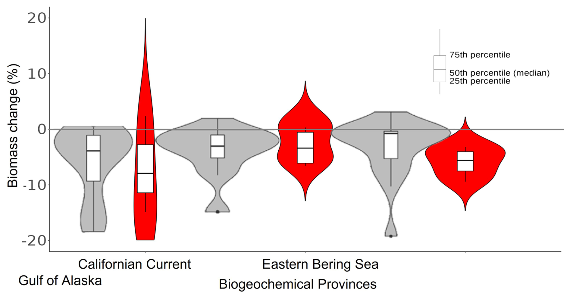
Figure 9 Biomass change associated with the northeastern Pacific MHW (2013–2016) per biogeochemical province. Grey violin plots correspond to results from Cheung and Frölicher (2020), while the red ones correspond to our hindcast EcoTroph-Dyn simulation with α=0.2 (figure adapted from Cheung and Frölicher, 2020).

One of the main uncertainties in modelling MHWs in EcoTroph-Dyn is the assumption of the resilience of the biomass spectrum to MHWs, i.e. parameter α. It is important to note that the α values applied in this study were chosen arbitrarily, albeit reasonably, and were able to capture a broad range of potential responses to MHWs. It would therefore have been valuable to test EcoTroph-Dyn against other MHWs in the world ocean in order to acquire better estimates of the α parameter and more reliable results regarding the consequences of MHWs. However, to date, few MHWs are as well studied as the Blob, limiting these analyses. As discussed in Guibourd de Luzinais et al. (2024), given the diversity of ecosystem functioning, there is no reason why communities in different ecosystems, biogeochemical regions or trophic levels should have the same capacity to resist MHWs. Thus, we encourage future studies to use various observational data on the impacts of MHWs across the ocean (if available) to better estimate the α parameter as a function of different ecosystems, biogeochemical regions or trophic levels in order to reduce the uncertainties in projections.

Here, we focussed solely on the direct impacts of MHWs occurring during the year's warmest month via thermal stress, resulting in species mortality (Oliver et al., 2021; Smith et al., 2023). However, MHWs in other seasons can also have consequences on populations by affecting a specific stage of the life cycle of certain species (Crickenberger and Wethey, 2018; Oliver et al., 2021; Smith and Thatje, 2013). For example, MHWs that stress adult breeders can lead to a decrease in reproductive investment and, consequently, fewer, smaller and lower quality gametes (e.g. Shanks et al., 2020), resulting in a loss of abundance and biomass of some species (Johansen et al., 2021). While taking seasonality into account will increase the number of detected extreme events, some may not have ecological consequences (Oliver et al., 2021; Smith et al., 2023). Thus, our approach can be seen as conservative and may underestimate the impact of MHWs. Nevertheless, we detected MHWs with potentially significant ecological impacts. Studying MHWs occurring in seasons other than summer would involve considering the phenological effects of MHWs. However, since the EcoTroph-Dyn model does not directly represent this phenological aspect of marine organisms, future studies can apply other approaches that explicitly represent seasonal processes such as spawning and migration to elucidate the effects of phenology.

Furthermore, uncertainties in our results arise from the environmental drivers of EcoTroph-Dyn. In our current investigation, EcoTroph-Dyn was driven by satellite data. For the NPP forcing variable, we implemented the EPPLEY-VGMP algorithm (Behrenfeld and Falkowski, 1997; Morel, 1991), which, like other algorithms such as CbPM and CAFE, derives NPP from satellite-derived estimates of Chl a and SST. First, in this study, we did not consider the “with” and “without” MHWs scenarios for NPP. Acknowledging that MHWs generally increase NPP at high latitudes while decreasing it at low latitudes (Arteaga and Rousseaux, 2023; Bouchard et al., 2017; Le Grix et al., 2022; LeBlanc et al., 2020), we may have overestimated MHW impacts on ecosystem functioning at high latitudes and underestimated their impact at low latitudes. Furthermore, the variability and uncertainty in the estimation of the NPP by satellites directly affects the reliability of our results. In EcoTroph-Dyn, as well as in other marine ecosystem models, ocean primary production (and its related phytoplankton biomass) plays a crucial role in both sustaining and constraining the biomass of higher trophic levels (e.g. Blanchard et al., 2012; Carozza et al., 2016; Cheung et al., 2011; Jennings and Collingridge, 2015). However, there exists significant variability in NPP estimation among satellite NPP algorithms (Milutinović and Bertino, 2011; Westberry et al., 2023). These discrepancies are particularly pronounced over continental shelves and oligotrophic gyres, primarily due to variations in model parameterisation and growth rate representation (Milutinović and Bertino, 2011; Westberry et al., 2023). Second, in this study, in order to propose a suitable representation of the world ocean, we use an interpolation method to reconstruct an incomplete NPP time series. The interpolation was constrained by the minimum and maximum satellite data values of the NPP observed over their respective time series to ensure reliable interpolation and reduce potential bias. Third and lastly, in this study, we duplicated the NPP monthly values to enable the EcoTroph-Dyn to run with 15 d time steps. This duplication may have smoothed marine ecosystem responses to the historical changes in marine environment; however, it has not changed trends and the conclusions of our results. Consequently, elucidating the sources of the current uncertainty associated with satellite-derived NPP and refining these estimates pose significant challenges in comprehending the responses of marine food webs to MHWs.

Moreover, EcoTroph-Dyn does not account explicitly for species; thus, we could only assess aggregated food web responses to MHWs. The model projected that the aggregated response across species is expected to be negative, although it is known that some species would exhibit positive effects from MHW occurrence (Cavole et al., 2016; Smith et al., 2023; Suryan et al., 2021; Wernberg et al., 2016). To be cautious, we considered various loss rate scenarios to obtain a complete range of responses from marine ecosystems. Running the aforementioned five MHW-induced loss rate scenarios, we found that the aggregated resistance capacities α had a significant (ANOVA, p value < $\mathrm{2}\times {\mathrm{10}}^{-\mathrm{16}}$) and large effect. All scenarios are consistent with each other, with an increasing biomass loss over marine ecosystems with decreasing resistance capacities (increasing α). Even though the global impact of MHWs is negative, species-explicit modelling could improve our understanding of how various impacts of climate change and species-level responses will affect trophodynamics and ecosystem structure and function.

4.4 Implications and future research

In our study, we highlighted the specific impacts of MHWs on ecosystem structure and function, particularly through the case study of the MHW known as “the Blob” (the longest and strongest period of abnormal temperature ever recorded (Collins et al., 2019; Oliver et al., 2021)). The anomalously low wind during the 2013–2014 winter induced the anomalously weak Ekman transport of colder water from the north and, coupled with anomalously low air–sea heat exchange, triggered the Blob (Bond et al., 2015). Furthermore, these processes as well as the El Niño Southern Oscillation (ENSO) have already contributed to the increased average duration and intensity of MHWs in the northeastern Pacific Ocean. Given that projections for the 21st century indicate that ENSO events will increase in intensity and frequency (Holbrook et al., 2020; Oliver et al., 2021), events such as the Blob are expected to occur more frequently (Holbrook et al., 2020; Oliver et al., 2021). This underscores the need for ongoing research to better understand how MHWs disrupt ecosystems. Finally, throughout the 21st century, ecosystem responses will depend on the ability of communities to adapt to the long-term increase in ocean temperature and their ability to withstand short-term extreme temperatures (Johansen et al., 2021). Therefore, to enhance our understanding of how marine ecosystems will respond to climate change, future studies should focus on potential scenarios of adaptive responses to future climate and associated MHWs. The EcoTroph-Dyn model is a tool to understand the ecological consequences of MHWs at global and local scales and to project their impacts under future scenarios. However, the model focuses on aggregated energy flows between trophic groups, while ecological responses to MHWs of species in each group may vary substantially. Some species may acclimatise or adapt to MHWs. Consideration of the potential acclimatisation/adaptation in the model requires the development of specific adaptation scenarios and model settings in addition to the model settings presented here.

5 Conclusions

Utilising the EcoTroph-Dyn trophodynamic framework for MHWs, we highlighted substantial and latent repercussions of MHWs, notably biomass loss and biomass flow alteration, which are particularly consequential for higher TLs. As a result, the recovery/restoration time can extend over several years, if not decades. The EcoTroph-Dyn model demonstrates its capacity to characterise the impacts of MHWs on ecosystem structure and functions, with a slight underestimation of the magnitude of the impacts when the model is applied to examine the Blob MHW. However, considering the dynamics and characteristics of current and future MHWs, it can be anticipated that ecosystems might not be afforded the necessary temporal window to recover between successive MHW events, which can significantly disrupt long-term trends associated with climate change.

Appendix A

A1 MHW characterisation and detection

To characterise MHW in each ocean spatial cell, we analysed daily SST observations from the NOAA's AVHRR data (DOC/NOAA/NESDIS/NCDC, 2008; https://www.ncei.noaa.gov/access/metadata/landing-page/bin/iso?id=gov.noaa.ncdc:C00680, last access: 3 May 2022). We defined MHW as a discrete, prolonged and anomalously warm water event when the daily SSTs exceed an extreme temperature threshold value for at least 5 consecutive days (Hobday et al., 2016). The extreme temperature threshold value was calculated for each 1° latitude × 1° longitude spatial cell as the 90th percentile of daily SST from the 30-year historical time series from January 1982 to December 2011. We did not calculate threshold values by season; thus, MHW events were identified by a single threshold across the year. As a result, we detected MHWs mostly occurring during the year's warmest months (see Fig. A1a for a schematic explanation). This approach to identifying the MHW threshold represents biological extreme temperature in the local (spatial cell) context. It is appropriate to assess the direct mortality associated with MHWs (Oliver et al., 2021). We determined a reference average sea surface temperature (SST average) for each spatial cell by analysing data from 1 January 1982 to 31 December 2011. Utilising this reference average SST, we classified each spatial cell into thermal classes, with each class representing a 1 °C increment of the reference SST average, ranging from −1 to 29 °C (refer to Fig. A1b). We used the R package heatwaveR, described at https://robwschlegel.github.io/heatwaveR/ (last access: 17 October 2022), to compute the MHW characteristics in each spatial cell from January 1982 to December 2021. Thus, we finally obtained MHW characteristics for each 1° by 1° of longitude and latitude ocean grid cell up to December 2021. The considered MHW characteristics are the threshold value defining MHWs, MHW's duration (in days), category and intensity (mean SST anomaly) and declaration of MHW days over the SST time series.

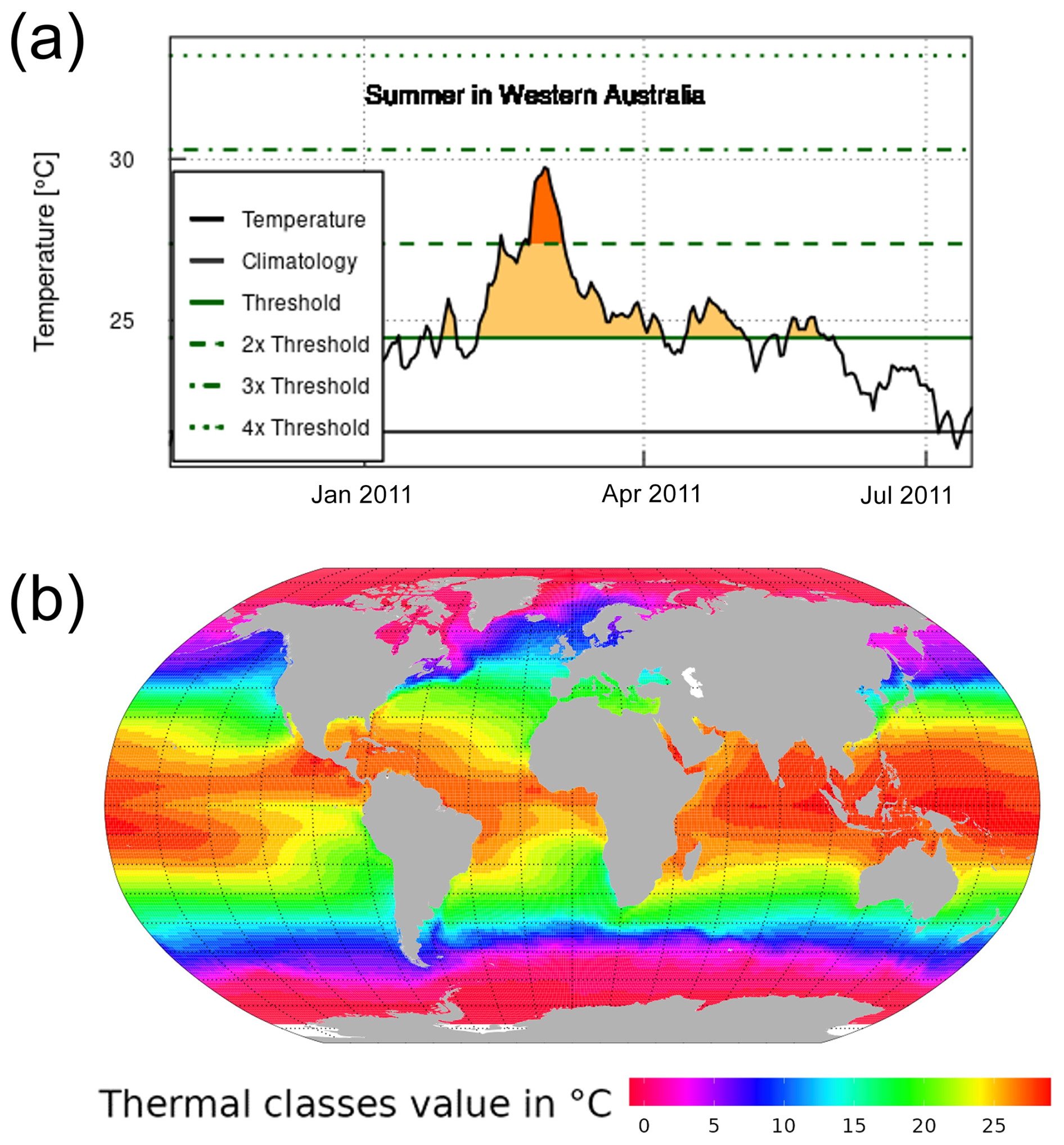
Figure A1 Marine heatwave detection method and reference average SST of each ocean cell. (a) Schematic explanation of MHW detection for a spatial cell. The solid horizontal green and black lines represent the extreme threshold value and the reference temperature, respectively. (b) A map of thermal classes of 1 °C intervals from −1 to 29 °C, categorised based on the reference temperature of each spatial cell over the period 1 January 1982 to 31 December 2011.

A2 Estimation of species distribution and associated thermal niche

We developed an algorithm depending on the MHWs' characteristics to express the loss rate of trophic transfers associated with MHWs. First, we identified a list of marine species from their occurrence records (3242 bivalves, 500 cephalopod species, 3116 crab species and 12 782 fish species), gathered from the publicly accessible databases OBIS (https://www.iobis.org, last access: November 2021), the Intergovernmental Oceanographic Commission (https://ioc-unesco.org, last access: November 2021), GBIF (https://www.gbif.org, last access: November 2021), FishBase (https://www.fishbase.org, last access: November 2021) and the International Union for the Conservation of Nature (https://www.iucnredlist.org/resources/spatial-data-download#marine, last access: November 2021). We then cleaned the data by removing duplicate entries, terrestrial occurrences and occurrences outside the known species habitat from the aggregated species occurrence dataset (Froese and Pauly, 2018). Additionally, we excluded zooplankton from the algorithm development due to limited evidence of direct mortality induced by marine heatwaves (MHWs), with observed responses mainly manifesting as range shifts and alterations in community structure (Arimitsu et al., 2021; Suryan et al., 2021; Winans et al., 2023). Marine mammals and seabirds were also omitted from the algorithm development, as their mortality linked to MHWs primarily stems from secondary effects such as diminished quality and quantity of food supply (Cavole et al., 2016; Piatt et al., 2020) rather than direct heat stress impact. Subsequently, the data were rasterised into a grid covering the global oceans (1° longitude by 1° latitude), denoting the historical presence of each species. Species with occurrence records in fewer than 30 cells were excluded from further analysis (Hernandez et al., 2006).

In a second step, we utilised an ensemble species distribution modelling approach (Asch et al., 2018; Reygondeau, 2019) at a 1° grid scale. Four environmental niche models (ENMs) were applied: Bioclim, Boosted Regression Trees models (Thuiller et al., 2009), Maxent (Phillips et al., 2006) and the Non-Parametric Probabilistic Ecological Niche model (Beaugrand et al., 2011), using global climatology satellite data (AVHRR). Model accuracy was assessed using the area under the curve (AUC) analysis of the receiver operating characteristic (ROC), discarding models with an AUC below 0.5 (Sing et al., 2005). The evaluation employed the pROC package in R (Robin et al., 2011). We then calculated the average habitat suitability index (HSI) weighted by the AUC values of each ENM for each spatial cell and species. An HSI threshold for each species was estimated using its prevalence. Spatial cells with an HSI below the threshold were deemed non-viable habitats.

Species' predicted thermal niches were quantified from spatial distributions using averaged satellite SST data (AVHRR) from 1982 to 2011. The average SST from 1982 to 2011 was recorded for each spatial cell above the HSI threshold. We then characterised the predicted thermal niche (histogram of all the average values of SST) and, more specifically, the upper temperature threshold for each species from the 95th percentile of the SST records where they were predicted to occur.

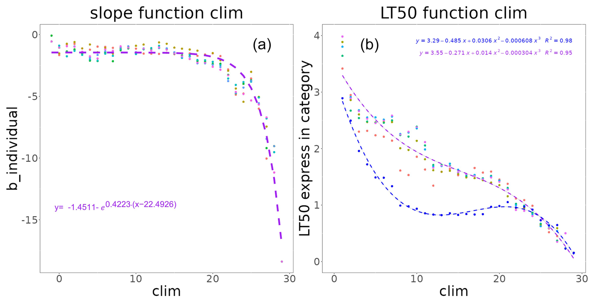
Figure A2 The coefficients correspond to thermal stress models for each reference temperature, with (1) corresponding to the Gompertz slope at the inflexion point coefficient b and (2) the MHW category that causes 50 % of species to undergo thermal stress (lt50), with blue and other colours corresponding to the trophic levels below 2.5 and above 2.5, respectively.

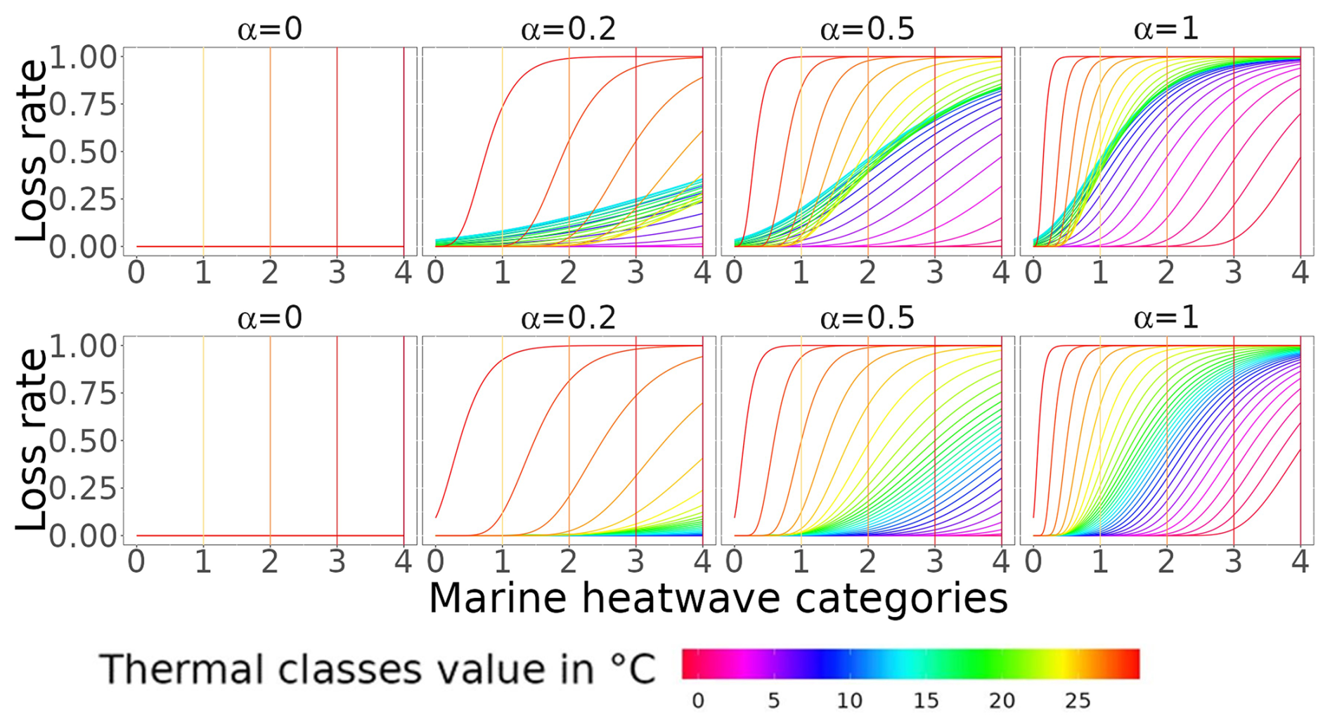
Figure A3 Loss rate associated with MHW occurrences, with the ecological hypothesis that MHW increases in intensity/category continuously challenging the aggregated response across species. On the plots, b is equal to 1. The top and bottom rows correspond to the loss rate of trophic level < 2.5 and trophic level > = 2.5, respectively.

A3 Additional loss rate associated with MHW

For each spatial cell belonging to each thermal class, we calculated the percentage of species in each trophic class exposed to thermal stress induced by MHW intensity above the estimated temperature threshold (95th percentile of the thermal niche). Matching MHW intensity in each spatial cell from 1981 to 2021 with species' temperature thresholds, we determined the percentage of species exposed to temperatures exceeding their thresholds. The thermal stress of a species was assumed to be dependent on the MHW category (1 to 4, based on SST anomaly) and species' trophic level (< 2.5, 2.5–3.0, 3.0–3.5, 3.5–4.0, 4.0–4.5, 4.5–5.0, > 5.0), estimated from FishBase and SeaLifeBase.

To obtain a continuous representation of the percentage of species undergoing thermal stress as the intensity of MHW increases, we decided to transform the discrete MHW categorisation (Hobday et al., 2018) to a continuous MHW intensity index as follows:

$$\begin{array}{}\text{(A1)}& {\mathrm{MHW}}_{\mathrm{cat},i}={\displaystyle \frac{\text{MHW mean anomaly},i}{\text{cat1 associated anomaly},i}}.\end{array}$$

The MHW mean anomaly was calculated as the difference between the MHW mean SST anomaly and the reference temperature of each thermal class (i), and “cat1-associated anomaly” is the mean threshold value used to identify category 1 MHWs in each spatial cell.

We fit the estimated percentage of species undergoing thermal stress with the MHW intensity index and species' trophic class to a non-linear function. A Gompertz function was selected after preliminary tests because it is better fitted to data than logistic or other mathematical functions with similar shapes. The Gompertz function is expressed as

$$\begin{array}{}\text{(A2)}& \begin{array}{rl}& \text{percentage of species undergoing thermal stress}=\\ & {\exp }^{-{\exp }^{b\mathit{\_}t{l}_i\cdot \left({\mathrm{MHW}}_{\mathrm{cat},i}-\mathrm{lt}\mathrm{50}\mathit{\_}t{l}_i\right)}}.\end{array}\end{array}$$

We estimated the parameters b_tl_i, lt50_tl_i and MHW_cat,i for each thermal class i. The parameters b_tl_i and lt50_tl_i correspond to the slope of the function and the index of marine heatwave intensity (MHW_cat,i) at which 50 % of the species are undergoing thermal stress, respectively.

For each thermal class i, parameters b_tl_i and lt50_tl_i were expressed as (see Fig. A2)

$$\begin{array}{}\text{(A3)}& b\mathit{\_}t{l}_i=-\mathrm{1.4511}-e^{\mathrm{0.4223}\cdot \left(i-\mathrm{22.4926}\right)},\end{array}$$

$$\begin{array}{ll}{\displaystyle }\mathrm{lt}\mathrm{50}\mathit{\_}t{l}_i& {\displaystyle }=\mathrm{3.29}-\mathrm{0.485}\cdot i+\mathrm{0.0306}\cdot i^{\mathrm{2}}-\mathrm{0.000608}\cdot i^{\mathrm{3}}\\ {\displaystyle }& {\displaystyle }\text{when trophic level}<\mathrm{2.5}\end{array}$$

and

$$\begin{array}{}\text{(A4)}& \begin{array}{rl}\mathrm{lt}\mathrm{50}\mathit{\_}t{l}_i& =\mathrm{3.55}-\mathrm{0.271}\cdot i+\mathrm{0.014}\cdot i^{\mathrm{2}}-\mathrm{0.000304}\cdot i^{\mathrm{3}}\\ & \text{when trophic level}>=\mathrm{2.5}.\end{array}\end{array}$$

Finally, to move from the thermally stressed stage to the loss rate (η_ι), we assumed that species were continuously challenged by MHW-increased intensity (Fig. A3 for schematic differences), expressed as

$$\begin{array}{}\text{(A5)}& {\mathit{\eta }}_i={\exp }^{-{\exp }^{b_i\cdot \mathit{\alpha }\cdot \left({\mathrm{MHW}}_{\mathrm{cat},i}-\frac{\mathrm{lt}{\mathrm{50}}_i}{\mathit{\alpha }}\right)}}\cdot \mathit{\beta }.\end{array}$$

We explored the sensitivity of the results to species' acclimation capacity to MHW conditions by assuming that acclimation reduces the mortality rate due to species' exposure to thermal stress. We tested four acclimation capacity settings represented by the values of the coefficient α. These settings are full acclimation (α=0; no mortality due to thermal stress), partial acclimation (α=0.2, 0.5; 20 % and 50 % of the species die because of thermal stress, respectively) and no acclimation (α=1; all species die when they are under thermal stress). We also related the loss rate to the MHW duration over the fortnight by assuming that the duration increases the mortality rate. The duration of MHW is represented by β and ranges from β=0 (no MHW) to β=1 (MHW lasting 15 d of the fortnight) (see Sect. 2.3.2 for β computation).