Development of a statistical model for global burned area simulation within a DGVM-compatible framework

Fire-enabled Dynamic Global Vegetation Models (DGVMs) play an essential role in predicting vegetation dynamics and biogeochemical cycles amid climate change, but modelling wildfires has been challenging in process-based biophysics-oriented DGVMs, regarding the role of socioeconomic drivers. In this study, we aimed to build a simple global statistical model that incorporates socioeconomic drivers of wildfire dynamics, together with biophysical drivers, within a DGVM-compatible framework. Using monthly burnt area (BA) data from the latest global burned area product from GFED5 as our response variable, we developed Generalized Linear Models to capture the relationships between potential predictor variables (biophysical and socio-economic) that are simulated by DGVMs and/or available in future scenarios. We used predictors that represent aspects of fire weather, vegetation structure and activity, human land use and behavior and topography. Based on an iterative process of choosing various variable combinations that represent potential key drivers of wildfires, we chose a model with minimum collinearity and maximum model performance in terms of reproducing observations. Our results show that the best performing (deviance explained 56.8 %) and yet parsimonious model includes eight socio-economic and biophysical predictor variables encompassing the Fire Weather Index (FWI), Monthly Ecosystem Productivity Index (MEPI), Human Development Index (HDI), Population Density (PPN), Percentage Tree Cover (PTC), Percentage Non-Tree Cover (PNTC), Number of Dry Days (NDD), and Topographic Positioning Index (TPI). When keeping the other variables constant (partial residual plots), FWI, PTC, TPI and PNTC were positively related to BA, while MEPI, HDI, PPN, and NDD were negatively related to BA. While the model effectively predicted the spatial distribution of BA (Normalized Mean Error = 0.72), its standout performance lay in capturing the seasonal variability, especially in regions often characterized by distinct wet and dry seasons, notably southern Africa (R²= 0.72 to 0.99), Australia (R²= 0.68) and South America (R²= 0.75 to 0.90). Our model reveals the robust predictive power of fire weather and vegetation dynamics emerging as reliable predictors of these seasonal global fire patterns. Finally, simulations with and without dynamically changing HDI revealed HDI as an important driver of the observed global decline in BA.

1 Introduction

Globally, the impacts of climate change continue to manifest through extreme weather events and changes in weather patterns (Clarke et al., 2019). In Australia, the mean annual burned area in forested regions was about 1.8 million ha per year between 1988–2001, increasing to 3.5 million ha per year between 2002–2018, before the 2019–2020 “Black Summer” fires burned over 15 million ha nationally (Australian Government, 2020; Canadell et al., 2021). Similarly, in Canada, the 1986–2022 mean annual burned area was about 2.1 million ha, compared with the record-breaking 15 million ha burned in 2023 (Curasi et al., 2024; Jain et al., 2024; MacCarthy et al., 2024). These multi-decadal increases in burned area in both countries are consistent with evidence that climate change has intensified fire-conducive weather over time. Even though the effects of fires may be positive through contributing to selected natural ecosystem processes, large and frequent fires are often destructive and have far-reaching effects through loss of life, biodiversity, landscape aesthetic value, and increase in forest fragmentation and soil erosion (Bowman et al., 2017; Knorr et al., 2016; Nolan et al., 2022). The negative role of climate change in driving large and frequent burning has been well documented (Brown et al., 2023). However, climate change by itself does not fully account for the recent changes in global wildfire patterns as human activities are crucial drivers as well (Pausas and Keeley, 2021). For instance, recent empirical investigations have highlighted a notable 25 % reduction in burnt area extent over the past two decades, explicitly attributing this decline to human activities (Andela et al., 2017). Wu et al. (2021) argue that future demographic and climate patterns will cause an increase in burnt areas, particularly in high latitude warming and tropical regions. However, Knorr et al. (2016) concluded that, under a moderate emissions scenario, global burnt areas will continue to decline, but they will begin to rise again around mid-century with high greenhouse gas emissions. Cunningham et al. (2024), on the other hand reported that although total burnt area is declining globally, extreme fire events are increasing as consequence of climate change especially in boreal and temperate conifer biomes. Future global fire dynamics are clearly driven by the overarching interaction between human activities (altered ignition patterns, surveillance and management) and climate (Krawchuk et al., 2009). Accurately evaluating these factors through modelling could guide prescribing solutions that will ensure reliable fire management and attainment of Sustainable Development Goals (SDGs) (Koubi, 2019; Robinne et al., 2018).

Modelling continues to be an essential tool for comprehending and forecasting wildfire dynamics, founded on the intricate interplay among fire weather, vegetation, and human activities (Bistinas et al., 2014; Hantson et al., 2016). Models for wildfire can be process-based or statistical. While process-based models delve into the physics and dynamics of wildfires and vegetation, statistical models, on the other hand, tend to focus on analyzing historical data and identifying correlations to predict future wildfire events (Morvan, 2011; Xi et al., 2019). Process-based models such as fire-enabled DGVMs stand out in understanding interactions between climate, vegetation, and human activities in a mechanistic manner (Hantson et al., 2016; Rabin et al., 2017). However, their predictive skill is often not yet satisfactory (Hantson et al., 2020). The predictive skill of process-based models is often limited due to incomplete representation of fire drivers, uncertainty in parameterization, and difficulties in accurately simulating human-fire interactions (Archibald, 2016; DeWilde and Chapin, 2006; Hantson et al., 2020). Hence statistical approaches have often been used to evaluate human impacts on wildfires, in combination with weather and vegetation drivers (Haas et al., 2022; Kuhn-Régnier et al., 2021). Statistical approaches can effectively quantify and evaluate empirical relationships between fire occurrences and diverse predictors, providing flexibility in handling diverse data from multiple spatial and temporal scales. However, some authors reported that the application of statistical models for ecosystems other than the ones used in their derivation is often not reliable (e.g. Perry, 1998). This is mainly because statistical models assume that the relationship between predictors and responses is stationery and context dependent, which is not typical of fires that are stochastic in nature. Integration of mechanistic process-based techniques and statistical methods remains one common way forward to advance our understanding of fire dynamics.

The integration of DGVMs and statistical models increasingly benefits from remote sensing data (Dantas De Paula et al., 2020). Remote sensing provides spatially explicit observations, such as vegetation cover, leaf area index (LAI), and biomass, which are used to initialize, calibrate, and validate DGVM simulations (Yang et al., 2020). Meanwhile, statistical models help correct biases in DGVM outputs and enhance predictions by combining empirical relationships with mechanistic model results. This integration enables more reliable modelling of global wildfires, offering a macroscopic perspective, and allowing researchers to analyze large-scale patterns across diverse ecosystems (Doerr and Santín, 2016; Flannigan et al., 2009). The strength of modelling fires at a global scale lies in its ability to capture overarching patterns (spatial, seasonal and inter-annual) that might provide valuable insights for strategic wildfire control. While one can argue about the potential oversimplification of local factors and the challenges in representing fine-scale heterogeneity, global models do, on the other hand, excel in capturing and understanding the effect of climate change, partly because they capture large climatic gradients (Robinne et al., 2018). The ability to capture the interconnectedness of ecosystems and fire regimes on a planetary scale contributes to a more holistic approach to understanding global vegetation dynamics and carbon cycling (Bowman et al., 2013; Kelly et al., 2023). As such, studies on evaluating drivers of burnt areas at a global scale in the face of ongoing climatic shifts are crucial in ensuring sustainable management of vulnerable ecosystems.

There is a growing recognition of the significance of exploring both interannual and seasonal variations to comprehensively understand the dynamics of fire across diverse ecosystems (Dwyer et al., 2000), partly because of the strong seasonal dynamics of vegetation. Also, understanding seasonal cycles of fires helps to identify peak fire seasons, regions prone to seasonal outbreaks, potential shifts in fire regimes over time and facilitating adaptive management strategies (Carmona-Moreno et al., 2005). Incorporating monthly data in global fire modelling helps researchers to accurately capture seasonal variations in fire activity. Hence, global models developed using monthly data are necessary.

Recent efforts have seen global burnt area models based on Convolution Neural Network (CNN: Bergado et al., 2021), Random Forest (RF) and Generalized Additive Models (GAM) (Chuvieco et al., 2021) which are currently not easily integrated into DGVMs, although we note that recent work from Son et al. (2024) is an important step towards integration of an advanced recursive neural network in a DGVM. GLMs are easier to implement into DGVMs, and their partial residual plots show the relationships of each predictor with the response variable when all other drivers are kept constant, which facilitates a discussion of potential underlying mechanisms. The risk of overfitting can be minimized by only choosing potential driver variables that are mechanistically expected to play an important role and by choosing only a limited number of uncorrelated driver variables. Accordingly, Haas et al. (2022) developed a GLM for global burnt area with good model skill but without accounting for seasonal dynamics and without a focus on driver variables that can be predicted with DGVMs. Generally, most earlier fire modules in DGVMs such as the LPJ-Lmfire (v1) were informally parameterized to predict seasonal fire cycles and do not consider the fuller range of predictors available in a more rigorous statistical framework (Fosberg et al., 1999; Pfeiffer et al., 2013). Nurrohman et al. (2024) produced monthly fire predictions from downscaling of annual model outputs without building a statistical approach that is trained based on monthly inputs. This left an opportunity to improve burnt area models in DGVMs to accurately represent the detailed seasonal dynamics. To our knowledge, there haven't been any reports on a simpler and more efficient statistical model specifically crafted to capture the seasonal cycles of global burnt areas, while also being easily integrated into DGVMs. Closing this gap can best be facilitated by developing a statistical model based on variables pertinent to fire modelling, with the goal to later integrate it into DGVMs. This integration can efficiently enhance our comprehension of inadequately understood factors while leveraging the potential of finely detailed temporal resolution burnt area datasets.

The main aim of this research is to build a parsimonious statistical model for global seasonal burnt areas that can be integrated into a DGVM. The specific objectives are to (1) to improve our understanding of major drivers of global burnt area dynamics, (2) to leverage a GLM for predicting global burnt areas using DGVM-compatible predictors and (3) to evaluate the interannual and seasonal cycles of burnt area extent, both globally and regionally.

2 Data and Methods

In this study, we used GLM to assess the drivers and distribution of global wildfires based on a combination of vegetation, weather, anthropogenic and topographic predictors. The spatial and temporal variability (interannual and seasonality) was also evaluated. Figure 1 provides an overview of the steps that were followed during modelling.

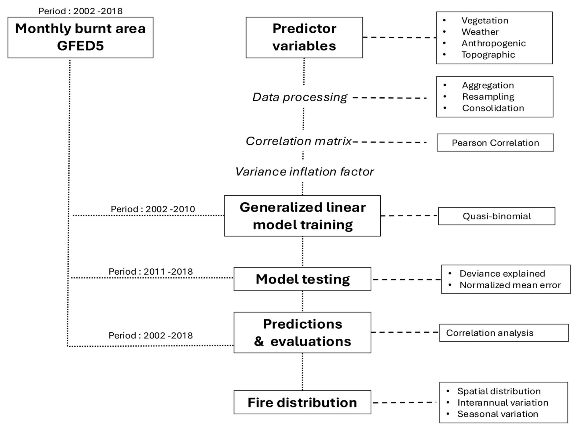
Figure 1 Study workflow showing an overview of steps followed in model training, testing, prediction and evaluation together with the outputs and time periods.

2.1 Fire data

Monthly BA data for the period 2002–2018 were derived from monthly mean fractional BA from the GFED5. We selected this data because of their improved ability to detect burnt area scars (Chen et al., 2023). GFED5 BA data are classified according to 17 major land cover types using the MODIS classification scheme. We used this land cover information to remove burnt area in cropland land cover type (type croplands and croplands/natural vegetation mosaic), to exclude the effect of cropland residue burning which we suppose is likely to have different drivers from burning in non-arable lands. The BA data comes at a resolution of 0.2° × 0.2°, therefore we aggregated it by a factor of 2 to a resolution of 0.0°. This was done for ease of processing at a global scale and at the same time to ensure that our outputs are DGVM integrable since they are commonly applied at 0.0° globally.

2.2 Predictor variables

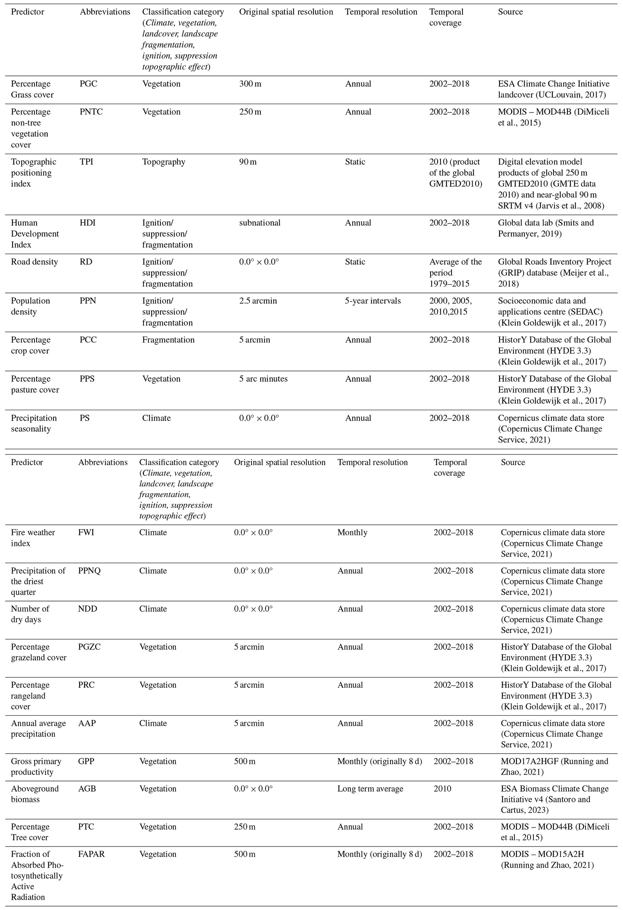
In this study, we only used variables which don't prohibit the use of the model for future projections. Whilst there are many possible variables that could be tried as predictors of fire, especially in terms of socioeconomics predictors, we restricted our selection to variables where: climate and vegetation variables typically available in a DGVM framework; socioeconomic variables with future scenario projections; and time-invariant topographic variables. Previous studies used several variables that we couldn't include due to lack of future scenario projections such as nighttime lights, cattle density (Forkel et al., 2019), vegetation optical depth (Forkel et al., 2019), lightning (Rabin et al., 2017), soil moisture (Mukunga et al., 2023), soil fertility (Aldersley et al., 2011). Consequently, we considered predictor variables that are compatible with DGVM integration to train the model effectively. The chosen predictor variables were categorized based on their representational nature and their roles in fire modelling (See Table 1).

Table 1 List of predictor variables that were considered in this study including their classifications, resolution (spatial and temporal) and the respective data sources.

2.2.1 Vegetation-related predictors

We used nine vegetation predictor variables to comprehensively evaluate their role on global fire distribution. These variables encompass Percentage Grass Cover (PGC), Percentage Non-Tree Cover (PNTC), Percentage Crop Cover (PCC), Percentage Graze Cover (PGZC), Percentage Rangeland Cover (PRC), Percentage Tree Cover (PTC), Fraction of Absorbed Photosynthetically Active Radiation (FAPAR), Aboveground Biomass (ABG), and Gross primary productivity (GPP). Previous work emphasizes the important role of vegetation on burnt area dynamics. For example, Thonicke et al. (2010), discussed the crucial role of vegetation structure in shaping fire occurrence, spread and intensity. PGC defines the land covered by grass, influencing fuel availability, while PNTC considers non-tree vegetation such as grass and shrubs, contributing to overall fuel dynamics. PCC reflects the presence of cultivated crops which have been found to suppress fire occurrence as they fragment the landscape acting and so act as a barrier to fire spread (Haas et al., 2022).

PGZC, PRC, PTNC and PTC were used to evaluate the relationship between landcover and burnt area distribution. Previous studies reported that land use/cover type has made a significant contribution to wildfire distribution (Gallardo et al., 2016; Villarreal and Vargas, 2021). GPP, AGB, and FAPAR were proxies for vegetation productivity and type, and fuel load. Also, some studies emphasized the varying effects of vegetation parameters on fire events (Bowman et al., 2020; Kuhn-Régnier et al., 2021).

To evaluate the role of fuel accumulation from the previous year on the burnt area, we derived the Monthly Ecosystem Productivity Index (MEPI) using monthly Gross Primary Productivity (GPP) data following Eq. (1). MEPI was originally defined in the work by Forrest et al. (2024). This index allowed us to quantify the relationship between vegetation growth, fuel accumulation and subsequent fire activity, providing a more nuanced understanding of the factors influencing fire dynamics.

$$\begin{array}{}\text{(1)}& \mathrm{MEPI}={\displaystyle \frac{{\mathrm{GPP}}_m}{max({\mathrm{GPP}}_m,{\mathrm{GPP}}_{m-\mathrm{1},},\mathrm{\dots },{\mathrm{GPP}}_{m-\mathrm{13}})}}\end{array}$$

where GPPm is the month's GPP, and the denominator is the maximum GPP of the past 13 months. Furthermore, we calculated additional metrics including GPP12 (the mean gross primary productivity over the previous 12 months), (FAPAR12) (the mean fraction of absorbed photosynthetically active radiation over the past 12 months), and FAPAR6 (the mean FAPAR over the last 6 months). These metrics serve to capture average vegetation productivity, serving as refined indicators of fuel accumulation. Kuhn-Régnier et al. (2021) highlighted the important role of antecedent vegetation as a key driver for global fires.

2.2.2 Topographic-related predictors

To evaluate how topography can influence the occurrence and spread of fires, we incorporated Topographic Positioning Index (TPI). Topography has been reported to be more influential in regions with complex terrain and microclimatic conditions (Blouin et al., 2016; Fang et al., 2015; Oliveira et al., 2014). Some studies used slope (Cary et al., 2006) and surface area ratio (Parisien et al., 2011) in their models and reported topography to marginally contribute to wildfire dynamics. However, recent studies reported some significant contributions of topography to global burnt area distribution when using the TPI (Haas et al., 2022). TPI is designed to encompass and evaluate the complex influence of terrain features, such as elevation and slope, on the distribution of burnt areas. Thus, TPI goes beyond simplistic representations of landscapes and offers a more nuanced perspective on how terrain characteristics contribute to the occurrence and extent of wildfires. Given the role of terrain on fire behavior and propagation patterns, the inclusion of TPI in this study allows for a comprehensive examination of wildfire distribution.

2.2.3 Anthropogenic influence predictors

To capture the impact of anthropogenic factors on both fire ignition and suppression, we adopted the Human Development Index (HDI), Population Density (PPN), and Road Density (RD). The inclusion of HDI aims to encapsulate human influence on ecological landscapes, thereby affecting the dynamics of both ignition and suppression processes. HDI is a composite index developed by the United Nations Development Program (UNDP) to assess long-term progress in three basic dimensions of human development, including health (life expectancy at birth), education (mean years of schooling and expected years of schooling), and standard of living (gross national income per capita) (Uddin, 2023). HDI values range from 0 to 1, with higher values indicating higher levels of human development. Although HDI itself may not directly relate to fire occurrence, it stands as a valuable socio-economic indicator that significantly influences overall fire dynamics and management, like how Gross Domestic Product (GDP) has been used in other fire models (Perkins et al., 2022). To address the limitations of using GDP as a proxy for human development in predicting global fires, we opted for HDI. Previous research has utilized GDP for this purpose (Zhang et al., 2023), however, GDP is an indicator of a country's economic performance (Callen, 2008). In contrast, HDI is a broader socioeconomic indicator which evaluates a country or other administrative region's development status based on the critical factors of life expectancy, education, and income. We assume it acts as a proxy for factors such as investments and advancements in fire control methods, surveillance, technology, and outreach strategies increasing awareness, thus providing a more nuanced understanding of the socio-economic context shaping fire behavior than GDP. To evaluate model sensitivity to inclusion of HDI, we trained our model based on the three settings: including, excluding and holding HDI constant.

2.2.4 Weather-related predictors

We employed the Canadian Fire Weather Index (FWI) to capture the impact of fire weather on the distribution of wildfires. FWI is renowned for its comprehensive framework integrating diverse meteorological parameters to evaluate potential fire behavior and danger (de Jong et al., 2016). The FWI is widely adopted by fire management agencies facilitating informed decisions on fire prevention, preparedness, and suppression strategies. It has been shown to correlate well with burnt areas across the globe (Jones et al., 2022). We used the number of dry days (NDD) as a proxy for biomass production limitations. While it falls in the category of weather-related fire predictors, in this study it's an indirect indicator of how moisture availability can affect available combustible vegetation. We incorporated additional covariates capturing seasonal and annual weather dynamics that influence fires, including Precipitation Seasonality (PS), and Annual Average Precipitation (AAP). The selection of these predictors was informed by their significance in previous global fire modelling studies (Chuvieco et al., 2021; Joshi and Sukumar, 2021; Le Page et al., 2015; Mukunga et al., 2023; Saha et al., 2019), as well as insights from seminal works such as that by Pechony and Shindell (2010).

2.3 Data processing

We harmonized the spatial and temporal resolution of the predictor dataset to conform to our analytical framework, which had a spatial resolution of 0.0° and a temporal resolution of one month. This involved employing techniques such as aggregation, resampling, and consolidation. For instance, while the native temporal resolution of FAPAR and GPP were 8 d, we transformed it into a monthly temporal resolution to align with our primary variable. Most predictors originally possessed an annual temporal resolution, except for FWI which was also available every month. For annual predictors, we replicated the same data for each month. Similarly, long-term variables like AGB, RD, and TPI were utilized every month to synchronize with the shorter-resolution predictors. PPN, which was available at a 5-year interval, was used monthly over the represented 5-year span.

2.4 Variable selection

To address variable collinearity, we conducted pairwise correlation analyses among predictor variables using the R statistical package (R Core Team, 2012). Following established guidelines by Dormann et al. (2013), we applied the conventional threshold of R>0.5 to enhance the model's efficiency. Moreover, we employed the Variance Inflation Factor (VIF) to evaluate collinearity among predictor variables, removing those with VIF values surpassing 5, as recommended by O'Brien (2007). Post collinearity tests, an additional 3 parameters were adopted to progressively select the best model, namely: (1) a simple (∼ parsimonious) model which comprise of a full suite of categories of covariate combinations (i.e. vegetation, climate, topography, ignitions), (2) the deviance explained value and (3) the Normalised Mean Square Error (NME) value as illustrated in the making of Burnt Area Simulator for Europe (BASE: Forrest et al., 2024).

2.5 Model training and testing

A quasi-binomial GLM was selected for modelling BA due to its capability to handle non-Gaussian error distributions, ease of transference to other modelling framework's ability to generate partial residual plots, i.e., the effect of each predictor in the model while the others are held constant (Bistinas et al., 2014; Haas et al., 2022; Lehsten et al., 2016). Residual plots were utilized to examine the magnitude and nature of each predictor's relationship with wildfire burnt area distribution. We used data from the period 2002–2010 for model training, the period 2011–2018 for model testing, and the full period 2002–2018 dataset for predictions and model evaluation. During model testing we compared the performance of the model on training data vs testing data to assess model robustness.

2.6 Model selection

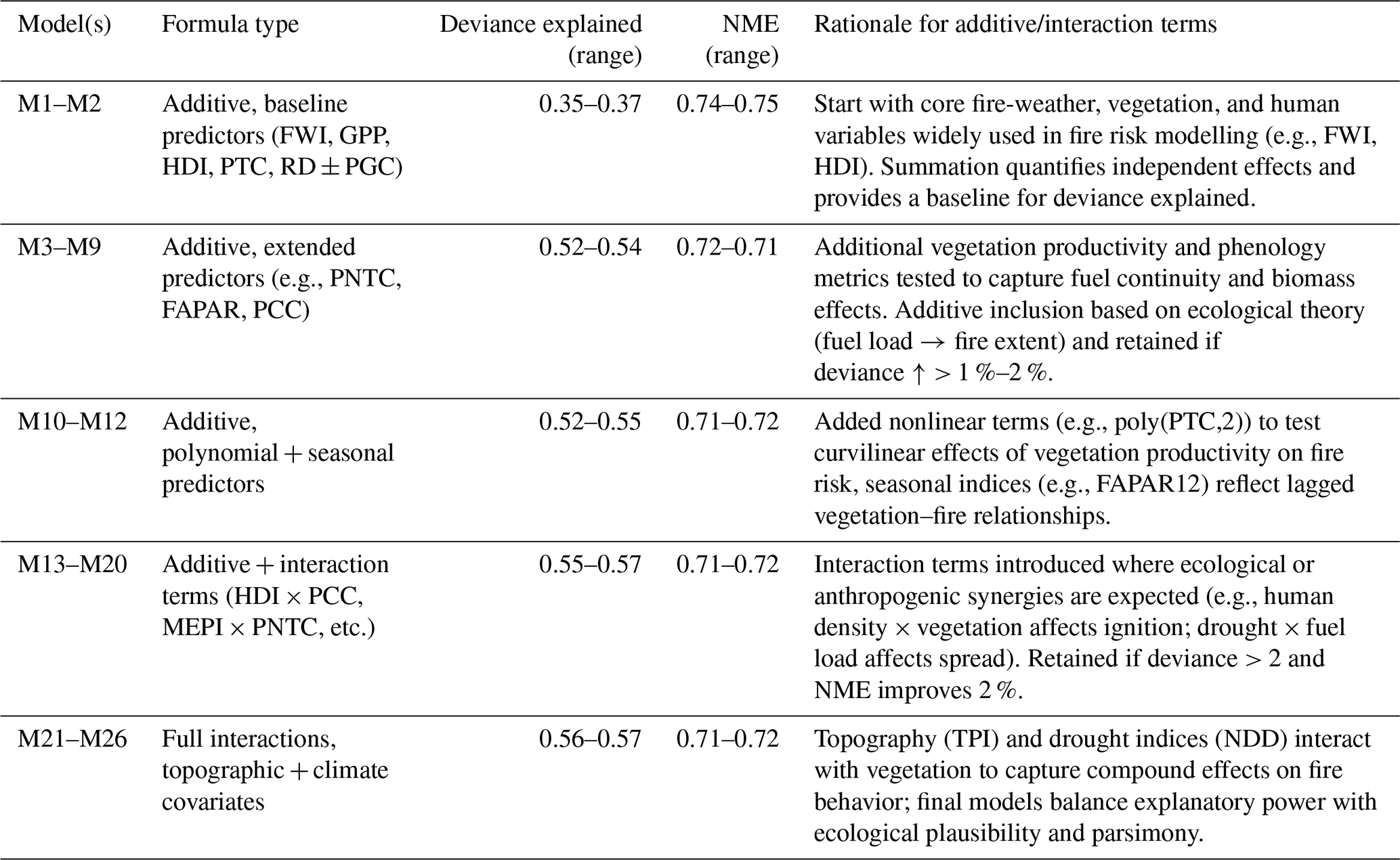
We employed a sequential model-building approach, beginning with additive structures (M1–M12) to estimate the independent contribution of climate, vegetation, and human variables on burned area (Table 2). This approach aligns with established fire risk modelling practices (e.g., Forrest et al., 2024). Additional predictors were introduced if they represented ecologically meaningful processes (e.g., drought severity, vegetation productivity) and improved model fit (deviance explained and Normalised Mean Error). Multiplicative interaction terms (M13 onward) were added only when fire ecology theory suggested synergistic effects (e.g., human ignitions under extreme weather, vegetation dryness and temperature) and retained if deviance explained improved. This stepwise approach ensures both statistical rigor and ecological interpretability rather than ad hoc formula selection.

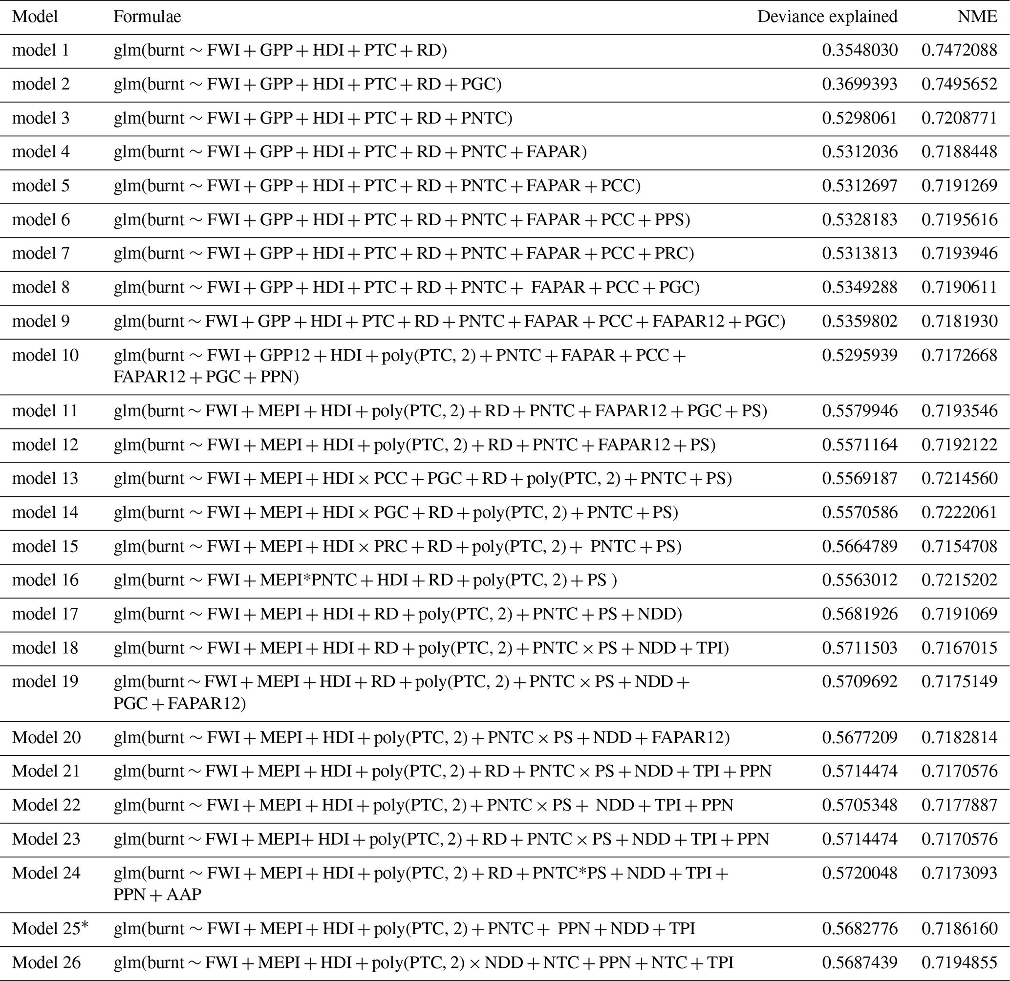
Table 2 Summary of models (M1–M26) with corresponding formulas, performance metrics, and rationale for predictor inclusion or interaction terms. Predictor additions were guided by ecological theory (e.g., fuel load, climate extremes, anthropogenic factors) and retained based on statistical improvements.

2.7 Model performance evaluation

Model performance was assessed using the NME following Kelley et al. (2013). NME serves as a standardized metric for evaluating global model performance, facilitating direct comparison between predictions and observations. The NME was calculated following Eq. (2).

$$\begin{array}{}\text{(2)}& \mathrm{NME}={\displaystyle \frac{\sum A_i{\mathrm{Iobs}}_i-{\mathrm{sim}}_i\mathrm{I}}{\sum A_i{\mathrm{Iobs}}_i-\mathrm{obs}\mathrm{I}}}\end{array}$$

The NME score was computed by summing the discrepancies between observations (obs) and simulations (sim) across all cells (i), weighted by the respective cell areas (A_i), and then normalized by the average distance from the mean of the observations. A lower NME value reflects superior model performance, with a value of 0 indicating a perfect alignment between observed and simulated values. After conducting a collinearity test, the models were systematically evaluated using various combinations of predictor variables. A total of 26 model runs were conducted, each incorporating different sets of variables while iteratively excluding some, to discern the extent to which each predictor explained variance when others were not included (see Table A1). We followed the stepwise approach of variable inclusion, exclusion, interaction terms, log transformations, and polynomial transformations as described by Forrest et al. (2024). While their analysis focused on Europe, our objective was to replicate and test the method at a global scale. To evaluate the reliability of the predicted interannual variability and seasonal cycles, we applied a regression function to determine the relationship (R²) between the observed and predicted trends using annual average data for the period 2002–2018. An R² of 1 shows good performance in our predictions and an R² of 0 shows poor performance in our predictions. To assess the trend in predicted interannual variability, we used the Mann-Kendall test (Kendall, 1975; Mann, 1945). This widely used method detects monotonic trends in environmental data. Being non-parametric, it works for all distributions, does not require normality, but assumes no serial correlation.

3 Results

3.1 Correlation between variables

We found correlated variables that we had to exclude from the analysis. Specifically, variables such as AGB, FAPAR12, FAPAR6, AAP, and RD were excluded due to their strong correlations with other variables (see Fig. 2). There were however some variables that correlated but had to be returned to the model due to their significant contribution to fire modelling and model performance. For example, NDD was strongly correlated to PTC (∼ −0.68), but both increased the variance explained by the full model.

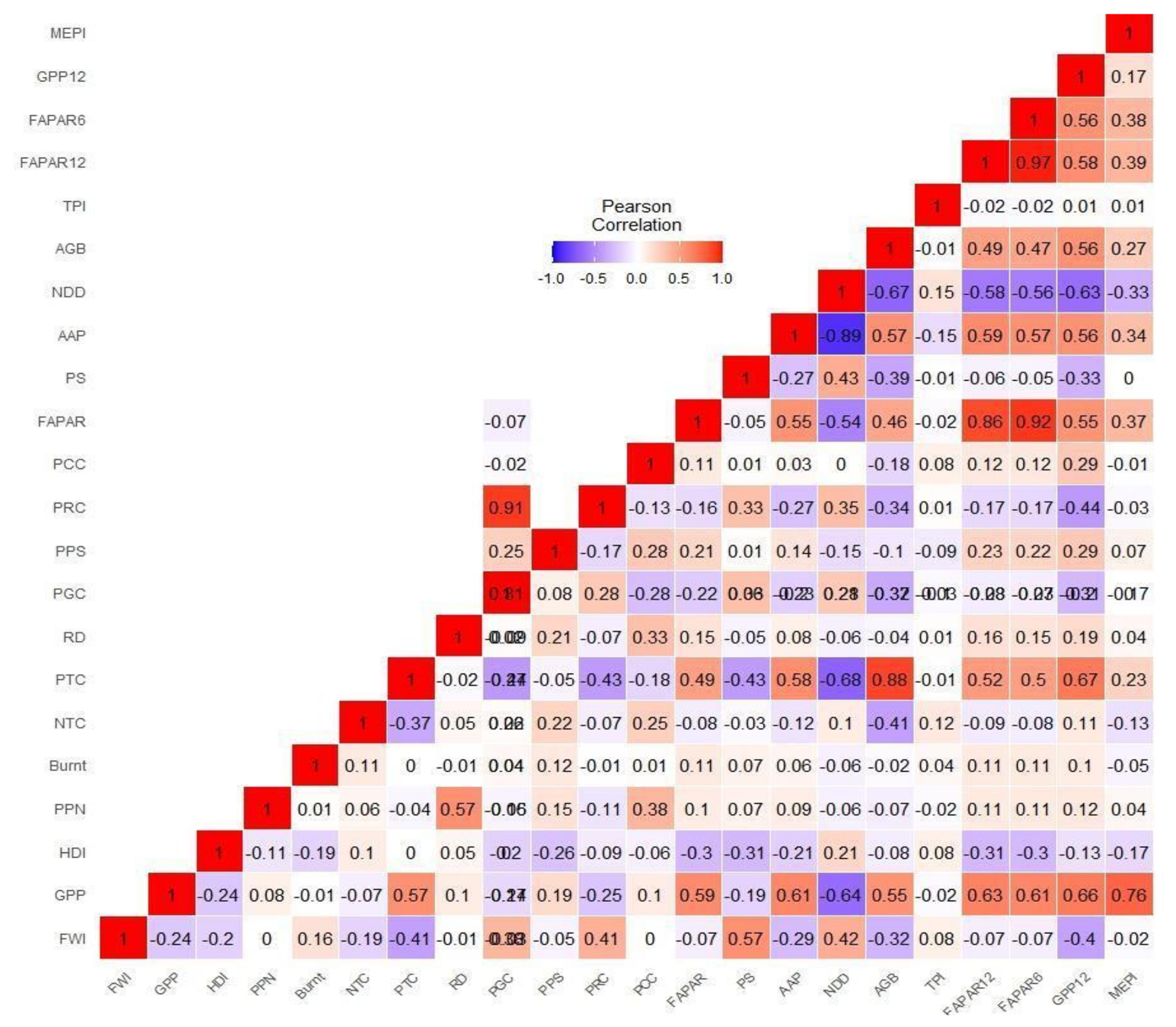
Figure 2 Correlation matrix of all the variables that were considered for modelling in this investigation.

3.2 Optimal model selection and GLM results

The initial models (model 1 to model 3) progressively include more variables and substantial improvement is observed in model 3 which explained 52.98 % following the inclusion of PNTC. Models 4 to 8 involve adding vegetation (FAPAR) and various land use types (PCC, PPS, PRC, PGC). This is accompanied by marginal improvement in deviance explained, indicating these factors provide some additional predictive power but are not as impactful as existing vegetation covariates (such as GPP). Models 10 to 12 introduce polynomial terms for PTC. This results in an increase in performance explaining 55.88 % in model 12. Models 13 to 16 incorporate interactions between HDI and land use types (e.g., PCC and PRC), resulting in marginal improvement in performance with the highest recorded in model 15 which explained 56.65 %. Models 19 to 26 fine-tune the overall performance by incorporating various variables and their interactions. Model 24, which includes a comprehensive set of climatic, vegetation, human, and topographic variables along with their interactions, achieves the highest performance as it explained 57.20 %. The marginal improvements observed in subsequent models indicate that while additional variables contribute to the model, the primary influencing factors were already identified by model 19, however it was not the simplest model (∼ parsimonious), and included variables for which future projections are currently unavailable (e.g., RD), due to the lack of established projection models or datasets. Since the main objective of the study was to produce a DGVM-compatible model, availability of future projections for these datasets was indispensable to model building. We removed some of the redundant variables till model 24 (∼ 11 variables), however, it was not as parsimonious as model 25 (∼ 8 variables). Therefore, model 25, which offers a balance of parsimony, simplicity, high deviance explained, and low NME, was selected as the best model in this analysis. Our results reveal that each predictor variable incorporated in the final analysis significantly predicted the distribution of wildfires (p<0.05), as outlined in Table 3.

Table 3 Summary of GLM coefficients for the final model, presenting t-values and p-values for predictors. The results indicate that all predictors in the final model were statistically significant for wildfire distribution (p<0.05).

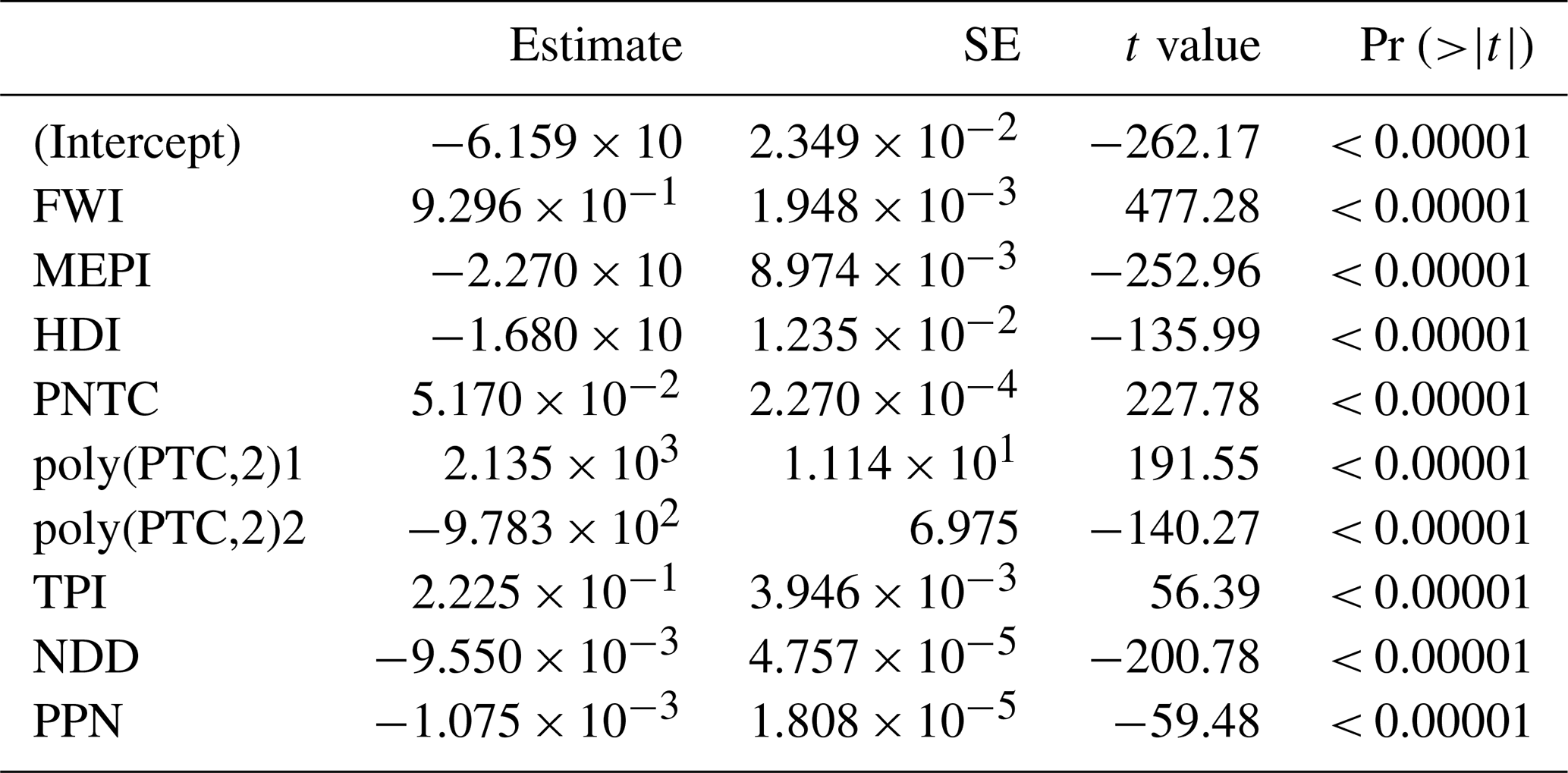
Our analysis results revealed the relationship between various predictors and BA distribution, as depicted in Fig. 3. Among the predictors studied, FWI, PNTC, PTC and TPI showed a positive relationship with BA distribution. Notably, FWI and PNTC showed particularly strong relationships, underscoring the substantial role of fire weather, fuel availability on the expansion of BA extent. Conversely, several predictors showed a negative relationship with BA distribution, including the MEPI, HDI, PPN and NDD. A polynomial of PTC shows a slightly bell-shaped relationship with burnt area fraction.

Overall, our observations highlight the critical role of factors such as fire weather, fuel availability, vegetation cover, climate conditions, and landscape characteristics in shaping BA distribution patterns. Figure 3 visually represents the differential relationship of these predictors on BA distribution, offering a comprehensive overview of the underlying mechanisms driving wildfire dynamics.

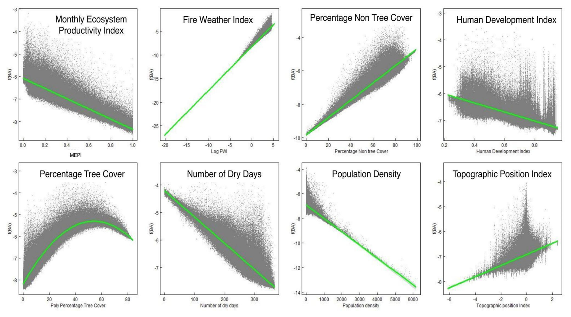
Figure 3 Partial Residual Plots illustrating the relationship between burnt Areas (BA) and the eight final predictor variables. These plots show the effect of each predictor while the others are held constant (Larsen and McCleary, 1972). Predictor variables were Monthly Ecosystem Productivity Index (MEPI), Fire Weather Index (FWI), Percentage Non-Tree Cover (PNTC), Human Development Index (HDI), Percentage Tree Cover (PTC), Topographic Position Index (TPI), Population Density (PPN) and Number of Dry Days (NDD).

3.3 Performance evaluation

The model demonstrated comparable performance across the training and testing datasets. Specifically, the training data yielded a deviance explained of 0.57 and an NME of 0.73, while the testing data yielded a deviance explained of 0.56 and an NME of 0.70. The close agreement between training and testing performance supports the robustness of the model and justifies its application to the full dataset, which we subsequently evaluated with respect to both spatial and temporal predictive capability.

The full dataset model demonstrated strong performance in predicting BA, as it explained 56.83 % of the variability in burnt area. Our model's performance, based on eight predictors and operating at a finer temporal resolution (monthly), is considered satisfactory and parsimonious. Overall, the model accuracy yielded an NME of 0.718, indicating a generally close correspondence between observed and predicted burnt area patterns.

The correlation analysis further shows significant variation in the strength of relationship between observed and predicted burnt area extent across the 14 GFED regions annually (Fig. 4a) and seasonally (Fig. 4b). These include: Boreal North America (BONA), Temperate North America (TENA), Central America (CEAM), Northern Hemisphere South America (NHSA), Southern Hemisphere South America (SHSA), Europe (EURO), Middle East (MIDE), Northern Hemisphere Africa (NHAF), Southern Hemisphere Africa (SHAF), Boreal Asia (BOAS), Central Asia (CEAS), Southeast Asia (SEAS), Equatorial Asia (EQAS) and Australia and New Zealand (AUST).

Our model overall performed poorly in predicting interannual variability as exhibited by a poor strength of relationship between the predicted trend when compared to the observed (R²= 0.24). This poor relationship was exhibited across most of the GFED regions (R²<0.50, Fig. 4a), except for the NHSA which showed strong similarities between the predicted trend and observed trend (R²= 0.55). This observation suggests that the combination of covariates that we incorporated in this model has limited strength in capturing global interannual variability in burnt areas.

Unlike the global interannual trends, there was a strong strength of similarity between observed and predicted seasonal cycles in most GFED regions (refer to Figs. 4b and A4). The model predicted better in GFED regions that are situated in Southern Africa, South America, Australia and Asia (R²>0.50). However, a few poor seasonal predictions were recorded in GFED regions situated in North America, North Africa and Europe as indicated by a poor relationship between observed burnt area and predicted burnt area (R²<0.50).

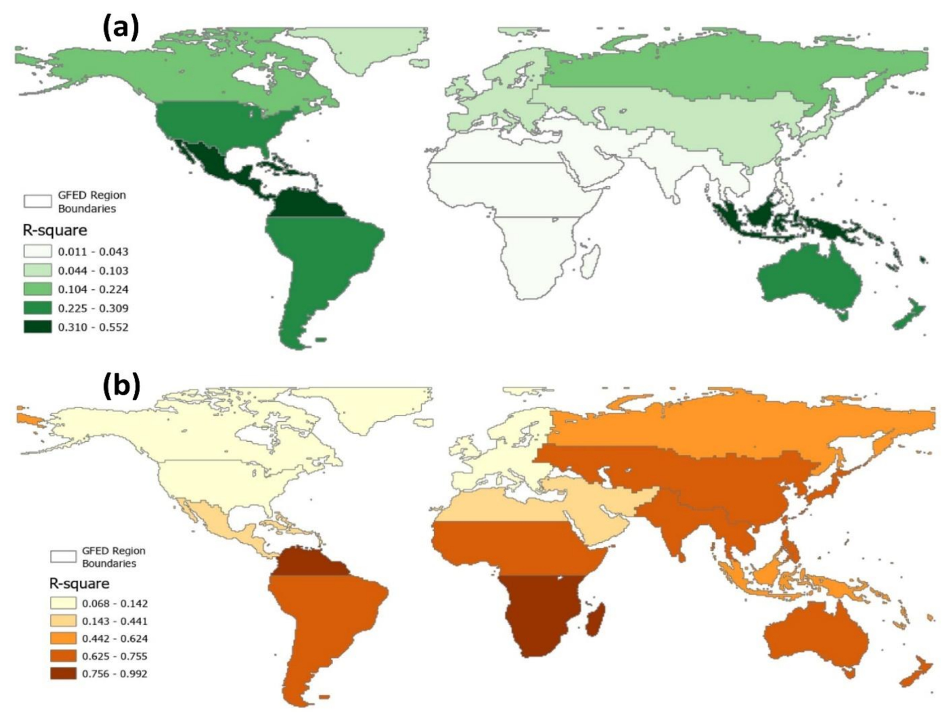
Figure 4 Evaluation of the selected model using observed burned area data from GFED5 predicted data (2011–2018). The maps show r-square values highlighting the model's performance for interannual (a) and seasonal variability (b) per GFED region.

Spatially, our model effectively captured the distribution of BA in the tropics and the southern hemisphere, demonstrating notable similarities between observed and predicted burnt area fractions on an annual basis (see Fig. 5). However, in extratropical regions, particularly in the northern hemisphere, instances of overprediction were observed. This discrepancy is evident in the inconsistencies between observed annual distribution patterns and those predicted by the model.

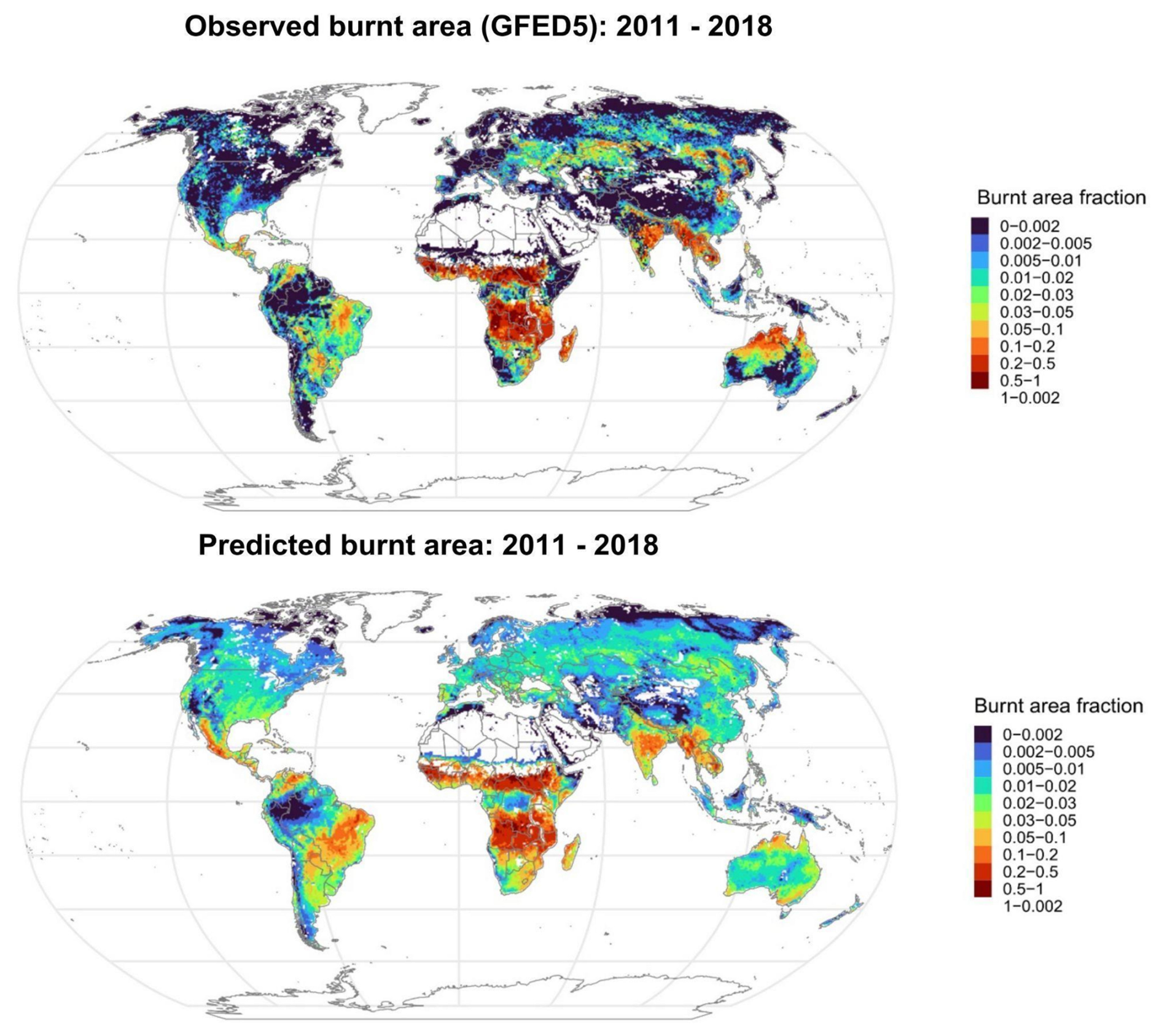
Figure 5 Annual burnt area fraction distribution map with the observed burnt area (top) and predicted burnt area (bottom).

3.4 Interannual distribution

Our analysis results revealed a substantial global decrease in burnt areas exceeding 1 million square kilometers from 2002–2018, with the peak decline observed in 2004 (see Fig. 6). This downtrend was reproduced by the model, but the model underestimated the interannual variability and the model-predicted decline was stronger than observed. However, it aligns with the decreasing patterns reported in earlier studies (Andela et al., 2017; Jones et al., 2022). Excluding and holding HDI constant in the model made the projected trend remain steady, suggesting the role of anthropogenic developments (increasing HDI over time) driving a downward trend in wildfire distribution.

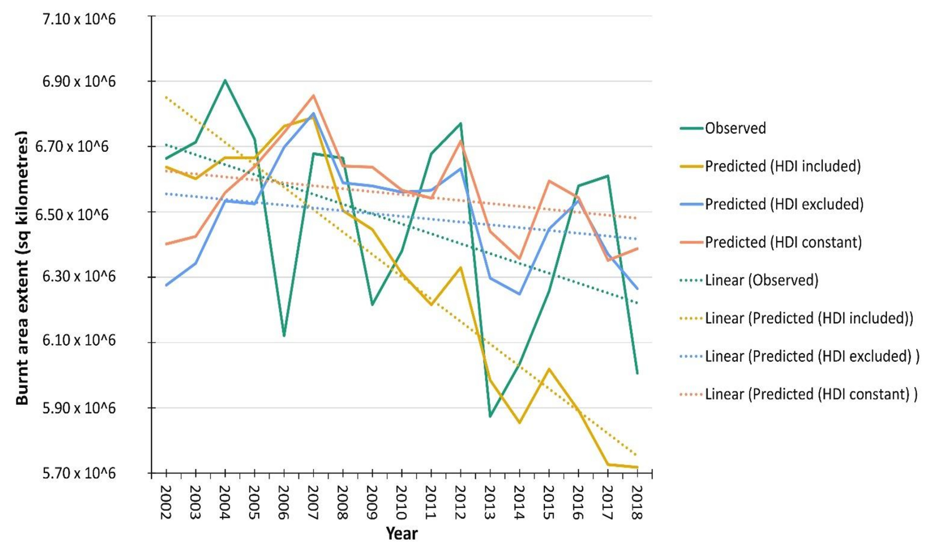
Figure 6 Interannual variability in burnt area extent showing the observed trend (based on GFED5 burnt estimates detection for the period 2002–2018) and model projections of the respective period under different HDI treatments: when HDI was excluded, included and held constant from the value of the first year in the model.

The Mann Kendall trend analysis further shows significant variation in the magnitude and direction of predicted burnt area extent across the 14 GFED regions (refer to Fig. 7 and Table A2). Five regions (SHAF, SHSA, NHAF, CEAS) predicted a significantly positive trend (p<0.05) in burnt area extent, while the other regions predicted no significant trends (NHSA, SHSA, MIDE, TENA, AUST, EURO, EQAS, CEAM, BONA, BOAS). Overall, the projected positive trend predominated in GFED regions situated in central and southern Africa, and central and southern Asia. In contrast, the Americas, Australia, and Europe demonstrated no significant trend, as illustrated in Fig. 7.

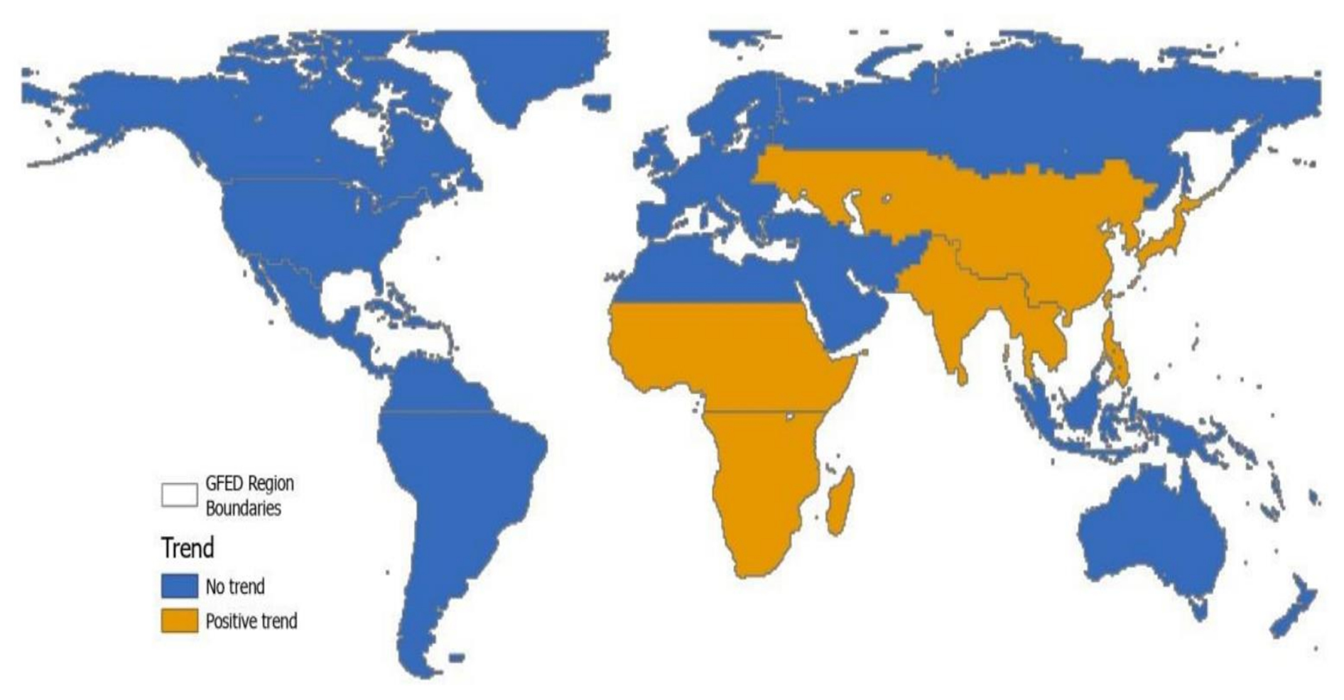
Figure 7 Variation in the direction of trend of interannual variability for burnt areas across different GFED regions.

3.5 Seasonal distribution

Our analysis results show that the global extent of BA shows an alternating seasonal cycle with strong peaks in February and August (see Fig. 8). The predicted pattern slightly underestimates the burnt area, however, appears to be closely knit with the observed trend (R²= 0.54).

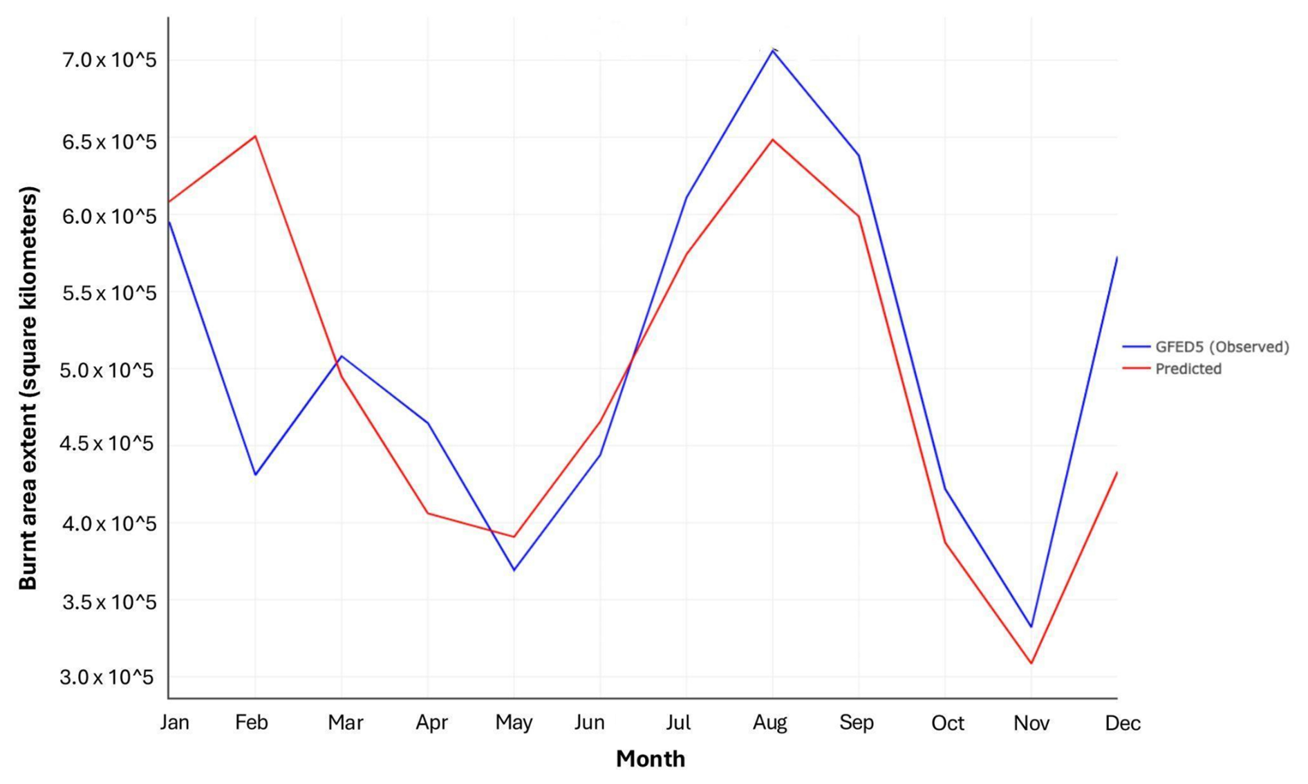
Figure 8 Global seasonal burnt area patterns showing the observed (GFED 5) and predicted burnt area extent.

4 Discussion

4.1 Main drivers of global burned area

We found that our candidate variables, namely FWI, PNTC, PTC, TPI, MEPI, HDI, PPN and NDD, had strong influence on burnt areas. FWI and PNTC exhibited a strong positive relationship with fire occurrence, underscoring the importance of conducive fire-weather conditions and combustible fuel in driving wildfire occurrence and spread. High PNTC is most likely related to high amounts of flammable vegetation, such as grasses and shrubs. Our findings that fire weather (∼ FWI) and fuel availability (∼ PNTC) influence burnt area extent align with previous studies (Andela et al., 2017; Bistinas et al., 2014; Forkel et al., 2019; Kuhn-Régnier et al., 2021). The other studies, however, did focus on the annual burnt area, not the seasonal cycle, which is also crucial to adapt to changes in fire risk.

Our results show that higher PNTC leads to higher burnt area fractions. In contrast, areas with lower PNTC show lower burnt area fractions. Areas with high PNTC typically consist of grasses and shrubs (∼ height <2 m), while areas with low PNTC are often characterized by trees. Grass and shrubs often encourage frequent burning much more than trees (Juli et al., 2017; Wragg et al., 2018). Conversely, low PNTC indicates high tree cover, which is often less flammable, leading to fewer fires. Though our findings support previous literature indicating that regions with abundant combustible vegetation and favorable fire-weather conditions are prone to frequent burning (Kraaij et al., 2018; Thonicke et al., 2010), we observed a surprising negative relationship between NDD and burnt area. Previous studies found a positive relationship between NDD and burnt area fractions (Haas et al., 2022), like our single-factor plots of NDD and burnt area in Fig. A3. This result most probably shows that relationships derived with annual data, as in the other studies mentioned here, cannot simply be transferred to seasonal fire predictions. Studies have shown that the effect of dryness on fire varies depending on vegetation communities in Mediterranean ecosystems (Cardil et al., 2019). Stott (2000) echoed similar sentiments for tropical environments, indicating the complex relationship between vegetation, dryness and fire. Our efforts to investigate this complex relationship through an interaction term did not significantly improve our model accuracy (∼ model 26). Hence, future studies may benefit from further exploring the complex relationship between dryness and vegetation at a global scale, particularly the effect of incorporating polynomial terms on correlated predictors in a linear model.

Our findings revealed that HDI, MEPI and PPN are negatively associated with trends in global fire extent. For HDI, our findings imply that technological advancements, improved surveillance systems, and effective mitigation efforts play a significant role in limiting the extent of burnt areas. Contrary to expectations based on Haas et al. (2022), PPN, which should correlate with more ignitions, does not appear to increase the burnt area extent (see Fig. 3). In fact, we observed that lower PPN corresponded to larger burnt areas, likely due to the impact of human activities on landscape fragmentation through road construction, and measures to suppress fires in human inhabited spaces to protect properties (Kloster et al., 2010). Saunders et al. (1991) observed that the response of fire to changes in PPN is governed by two opposing processes, an increase in population leads to more ignition sources, while simultaneously prompting greater fire management efforts to suppress fires. They further highlighted that fire suppression rates are highest in densely populated areas. This suggests that the scale (both spatial and temporal) of analysis may influence nature and extent to which PPN affects burnt area extent. Our results for the effect of PPN have important implications for DGVMs and land surface models. These models differ widely in the assumed effect of PPN, often using a unimodal response simulating BA annually, in some cases distributing the wildfires across seasons in a second step, using rather simplified assumptions (Teckentrup et al., 2019). Similarly, we anticipated a positive relationship between MEPI and burnt areas, as MEPI is indicative of ecosystem dryness and flammability. However, our findings revealed a negative relationship, indicating that other factors may be influencing the connection between MEPI and the extent of burnt areas. Our findings are in line with those of Forrest et al. (2024) who initially investigated the effect of this index on burnt areas in Europe. Unlike previous global studies that utilized annual GPP, our research employed a more refined measure, MEPI. Future research could benefit from evaluating the relationships between MEPI and burnt areas in other GFED regions and temporal scales.

4.2 Spatial variation in model performance

Our model exhibits stronger performance in predicting the spatial distribution of fires in southern Africa, Australia, and South America than in other world regions (See Fig. 4). The stronger performance in these areas is likely due to the well-defined and predictable fire regimes in these regions. Since fire activity here is strongly governed by distinct wet-dry seasonal cycles, which align closely with fire weather, enabling our model to capture these patterns effectively using linear functions (See Fig. A5), hence better model generalization.

Conversely, our model tends to overpredict fires in the northern hemisphere, particularly in North and Central America, as well as Asia. Performance here declines as fire regimes are more heterogeneous and driven by a combination of biophysical and anthropogenic factors (Chuvieco et al., 2021; Forkel et al., 2019). High interannual variability in burnt areas in these regions is due to irregular droughts, land use change, and fire suppression policies that make prediction more challenging for linear models. Additionally, the influence of snow cover, freeze-thaw cycles, and varied ignition sources in temperate and boreal regions further complicates seasonal pattern detection (Flannigan et al., 2009). Chuvieco et al. (2021) reported about this challenge when building global models. Thus, our findings build upon existing models on global burnt area distribution. What sets our model apart from previous models is its ability to reliably identify global seasonal fire distribution patterns. This simplicity offers a notable advantage, as it facilitates more nuanced interpretation and implementation of DGVMs compared to annual models.

4.3 Attribution of global trends

Previous studies have improved our understanding of drivers of fire but differ in approach and attributional focus for fire trends. For instance, Joshi and Sukumar (2021) employed region-specific multilayer neural networks to reveal spatially varying sensitivities between fire and socio-environmental drivers, providing strong spatial diagnostics but limited transparency on attributions of burnt area trends. Kraaij et al. (2018) provided detailed biome-level attribution of destructive fires by linking drought, fuel state and vegetation context in case studies (e.g., fynbos/plantation complexes), emphasizing vegetation and weather controls at local scales. Mukunga et al. (2023) used random-forest analyses to quantify the added value of human predictors for ignition probability, focusing on anthropogenic controls of ignitions rather than burnt area extent. Building on these approaches, our study contributes novel attributional insight because it explicitly integrates a compact set of DGVM compatible fire-weather and fuel indices (FWI, PTC, TPI, PNTC) with a socio-economic indicator (HDI) within a parsimonious statistical framework for burnt area trends. This allows direct attribution of directional effects (for example, the negative association between HDI and burnt area) across regions. Work by Andela et al. (2017), primarily attributed the decline in global burnt areas to agricultural expansion and intensification. Earl and Simmonds (2018) supported this view, adding that increased net primary productivity in Northern Africa also played a significant role. However, our results suggest that human development is a more important driver than agricultural expansion alone. Despite the conventional emphasis on agricultural factors, our attempt to incorporate cropland and rangeland fractions as predictor variables did not substantially enhance our understanding of this trend (model 5–10, Table 2). Interestingly, our analysis revealed that excluding the HDI from our model and holding it constant to the value of the first year predicted a steady trend that deviates from the observed negative trend in global fire extent and including HDI is partly followed by a decreasing trend (Fig. 5). This highlights the significant influence of HDI in projecting the purported negative global fire trend. Importantly, HDI is not uniform worldwide but varies substantially across regions and levels of socioeconomic development. For instance, in high-HDI countries, greater financial resources, infrastructure, and institutional capacity often translate into stronger investments in fire control technologies, improved surveillance systems, and more effective prevention campaigns. By contrast, in low and middle HDI countries, limited resources and weaker institutional frameworks may constrain fire management capabilities, resulting in greater reliance on natural fire dynamics or less formalized suppression efforts. As many countries continue to develop, it translates improvements in HDI and fire management strategies. Although strategies are often implemented independently and on a smaller scale, their cumulative impact on global fire trends is substantial. Thus, HDI serves as a broad socioeconomic indicator that we assume acts as a proxy for the combined effects of investments, advancements in fire control methods, surveillance, technology, and outreach strategies that increase awareness (Teixeira et al., 2023). Therefore, our model underscores the necessity for global initiatives aimed at enhancing fire control measures through comprehensive awareness campaigns, capacity-building efforts, resource mobilization, and the development and deployment of reliable surveillance technologies. By addressing these factors collectively, we can effectively mitigate the extent and severity of global wildfires, thereby safeguarding ecosystems and human livelihoods.

4.4 Interannual variability

Despite demonstrating the significant role of the HDI in predicting global fire trends, our model struggled to achieve high precision in forecasting interannual variability both globally (see Fig. 5) and within specific GFED regions (see Fig. A1). Recognizing that this limitation might stem from an inadequate representation of vegetation (fuel) dynamics, we incorporated FAPAR12 in models 9 to 12 (Table A1) and MEPI in models 11 to 26 (Table A1). Unfortunately, these adjustments did not enhance our ability to predict the interannual variability of wildfires. Studies have found a relationship between increased precipitation in the years preceding the fire season and fire activity in the drier savanna regions of Southern Africa (Shekede et al., 2024). Hence, we also explored the role of previous fuel accumulation on subsequent fire seasons using GPP12 in model 10, respectively. While this approach did not improve global interannual predictions, it showed a slight enhancement in deviance explained (from 0.5357 to 0.5461). This improvement might have been confounded by the effects of the fire-aerosol positive feedback mechanism in Africa (Zhang et al., 2023) and periodic El Niño conditions, which can affect rainfall patterns and lead to drier vegetation conditions, reducing the predictability of fire occurrence, especially with linear models (Shikwambana et al., 2022). We note that in the recent comparison of fire-enabled DGVMs in the Fire Model Intercomparison Project (FireMIP) project (Hantson et al., 2020), all models did a poorer job of matching the interannual variability than the spatial patterns by a considerable margin. The seven acceptably-performing models achieved a mean spatial NME (across all data and model comparisons) of 0.84 with respect to spatial patterns, but an NME of 1.15 for interannual variability. Our modelling efforts highlight the complexity of accurately predicting wildfire trends and underscore the need for future research to identify covariates that more effectively capture the interannual variability of fires at a global scale.

4.5 Fire seasonality

Globally, our model predicts a notable peak in burnt areas during February and August (Fig. 8). The February peak corresponds to dry conditions and fuel accumulation in northern hemisphere regions such as NHSA, NHAF, and MIDE (Fig. A2), with the complementary August peak occurring in regions such as SHSA, SHAF, and AUST. Our model predicts this with only two sub annual predictors - the logarithm of FWI and MEPI as already demonstrated for Europe by Forrest et al. (2024). This underscores the enduring influence of fire weather and vegetation growth and phenology as principal drivers of seasonal burnt area cycles, with factors such as moisture content in vegetation and soil, as well as humidity, playing pivotal roles in modulating ignition and fire extent within ecosystems. The seasonal forecasts generated by our model hold significant implications for guiding adaptive strategies, fire management and prevention at both regional and global scale.

The findings of this study exhibit robustness in capturing the global seasonal cycle (R²= 0.536, see Fig. 7), but notable exceptions were observed in North America, the Middle East and Mediterranean North Africa, and Europe (R²<0.50, see Fig. 8). This discrepancy could be attributed to the intricate climatic conditions inherent to these regions, which influence fires in a manner that eludes simple linear modelling. For instance, tropical regions with clear-cut wet and dry seasons tend to exhibit more regular fire cycles, largely governed by seasonal shifts in precipitation, temperature, and vegetation growth. These predictable patterns make them well-suited to linear modelling approaches (Kavhu and Ndaimani, 2022; van Der Werf et al., 2017). In contrast, extra-tropical areas experience more irregular and less seasonally driven fire activity. Here, the interaction of drought events, land management, and socio-economic drivers introduces variability that weakens model performance (Chuvieco et al., 2021; Forkel et al., 2019). Additionally, varied ignition sources in temperate and boreal zones disrupt consistent seasonal fire patterns (Flannigan et al., 2009). Given the parsimonious design of our model, with only eight predictors and only two of those on a monthly time step, we think that the model's performance is acceptable. Furthermore, this acceptable seasonal performance fills a gap in the available global fire models. To our knowledge there are no such models which are strongly data-constrained (i.e statistically fitted as opposed to empirical or processes-based) and which predict the seasonal cycle. The closest is SIMFIRE, which is fitted to observed data but which calculates annual burnt area and then distributes throughout the year using a prescribed seasonal cycle based on observed data (Rabin et al., 2017). So, whilst the work presented is not yet integrated into a DGVM, it represents a significant advance in this direction. This is particularly important given the comparatively poor performance of global fire models in predicting the seasonal concentration of burnt area (Hantson et al., 2020, Table 3). However, for certain regions, it might be possible to increase model performance by implementing further region-specific predictors and relationships. Accurate predictions regarding the seasonal dynamics of diverse GFED regions can facilitate the identification of temporal windows when fires are prevalent, thereby furnishing valuable insights for simulating carbon emissions in DGVMs.

4.6 Model limitations and excluding drivers of burnt area

Several covariates initially considered, such as landcover variables (∼ PCC, PPS, PRC, PGC), vegetation (∼ FAPAR) and socioeconomic (∼ RD), did not make it to the final model (See Table A1) despite their potential relevance identified in previous studies (Forkel et al., 2019; Hantson et al., 2015; Knorr et al., 2014; Pausas and Keeley, 2021; Perkins et al., 2022). The differences in our findings are related to differences in the statistical or modelling approach and the fact that most of these studies addressed annual BA patterns, not seasonal variations. Nevertheless, these other factors can clearly also be important for understanding fire dynamics, e.g., influencing fuel availability, landscape structure, and ignition sources. For instance, grazing lands can significantly impact fire behavior by altering fuel types and continuity, with areas used for grazing potentially reducing fuel loads (Davies et al., 2010; Strand et al., 2014). Similarly, FAPAR indicates vegetation health and productivity, affecting fuel moisture content and thus fire risk (Pausas and Ribeiro, 2013). However, these factors are apparently indirectly represented by the final model, as they are correlated to the driver variables in the final model. FAPAR, for example, is generally highly correlated with GPP. Furthermore, RD is associated with human-caused ignitions and fire suppression capabilities (Forkel et al., 2019). However, it was excluded here because its contributions were already effectively represented by HDI and PPN, which capture broader socioeconomic conditions and infrastructure impacts. Apart from that, Haas et al. (2022) observed a shift in the direction of contribution for covariates when PPN and RD are used together. Considering that we may not have future projections for RD unlike PPN, including the issue of collinearity, we decided to retain only PPN in our model. Furthermore, our attempt to include RD in our models 21, 23 and 24 (Table A1) yielded marginal improvements, which were not different from when we excluded it in model 25. Overall, the decision to exclude most of these covariates was aimed at reducing redundancy and multicollinearity, ensuring a balance between model complexity and predictive power. By focusing on more comprehensive variables with high explanatory power, the final model achieves robust explanatory power. However, the often-small differences in the deviance explained and the NME between different models imply that vegetation-fire modelers might also pick a slightly different set of variables for DGVM integration without using much predictive power.

While our research represents relevant efforts in developing a streamlined model capable of accurately capturing seasonal variations in global fire distribution, it's important to acknowledge certain limitations. The selection of covariates and the statistical model was constrained by the necessity for integration within DGVMs applied to predict future dynamics, potentially omitting some previously identified key predictors (∼ lightning frequency, gridded livestock densities) and modelling techniques (∼ Random Forest, Neural networks, XgBoost, CatBoost) for global fires (Forkel et al., 2019; Joshi and Sukumar, 2021; Mukunga et al., 2023; Zhang et al., 2023). This might contribute to observed shortcomings in our model's ability to predict spatial fire distribution in certain regions and to capture interannual variability across many parts of the world. Future investigations should aim to explore the inclusion of other established predictors and methodologies in global fire modelling once they become easily compatible with DGVM integration. Despite these challenges, our study possesses intrinsic value, and the developed model stands as a relatively simple tool for informing global seasonal fire predictions.

4.7 Next steps for DGVM integration, future directions and model improvements

To integrate the model presented here into a DGVM and enable future predictions, the remotely sensed variables of vegetation state (PTC, PNTC and MEPI) must be replaced with equivalent variables from the DGVM. DGVMs include GPP and the cover fractions of vegetation types required to calculate PTC, PNTC and MEPI, so these variables provide a robust and universal coupling strategy to capture the effect of vegetation on burnt areas. However, all model results are imperfect and biased to some degree, so the DGVM variables will not correspond perfectly with the remotely sensed ones used for model training. This error will propagate to the burnt area calculation and so this discrepancy should be investigated. In the likely event that this discrepancy is not small, the GLM should be refitted using the model-calculated variables to implicitly account for biases in the DGVM simulation, although the burnt area estimated will still be dependent on the DGVM's skill to capture certain dynamics and states. However, we note that our comparatively restricted variable set and simple GLM approach will be more straightforward to integrate and less sensitive to errors in the DGVM simulated state than machine learning approaches with larger suites of predictor variables. For example Son et al. (2024) achieved excellent correspondence with observed data using an advanced recursive neural network which was partially integrated into the JSBACH DGVM. However, only the fuel predictor was taken from the prognostically simulated JSBACH model state, other high importance dynamic predictors (including plant functional type cover fractions and both absolute values and anomalies of LAI and water content of four soil layers) are all determined from fixed input data – remotely sensed of climate reanalysis. Thus, in this case, the quality of the results from hypothetical full integration will be dependent on the ability of JSBACH to simulate many more variables correctly. The model presented here is tailored for integration into a DGVM by using only a few variables which can be robustly predicted, and, as a simple GLM in contrast to more complex machine learning methods, is less prone to overfitting and relying on correlations in the data which may not hold in the DGVM predicted state. Furthermore, the new model includes seasonal variations in burned area, which are not captured by all existing fire modules within DGVMs (Hantson et al., 2020).

In comparison to the vegetation variables, the inclusion of the other variables (FWI, HDI, PPN, NDD, TPI) is trivial as they can either be prescribed input variables or can be calculated from the climate input. Finally, to build a fully coupled vegetation-fire model, it is then necessary to include the effects of the simulated fire on the vegetation. For this step we can use the mortality and combustion components of fire models already available and integrated into DGVMs, for example the BLAZE model (Rabin et al., 2017) or the appropriate equations in SPITFIRE (Thonicke et al., 2010). These parameterizations may need to be adjusted to account for the different simulated burnt areas.

5 Conclusions

We present a parsimonious statistical model to simulate global burnt area on a monthly timestep thus including seasonal variations. This is an important advance as representation of the seasonal cycle is a weakness in global fire models, both in and out of DGVMs, and across different model types. Notably, this representation of the seasonal cycle was achieved with only two sub annual predictor variables. We found the drivers FWI, TPI, and PNTC are positively associated with BA, whereas MEPI, HDI, PPN, and NDD exhibit negative relationships, and PTC showed a unimodal response with strongest effect at intermediate tree cover. The diversity of these drivers underscores the multifaceted influence of both climatic and socio-economic drivers on fire dynamics. Our model explicitly accommodates these drivers, capturing how variations in climate, vegetation productivity, and human development interact to modulate fire occurrence and extent. Notably, the use of HDI to represent societal development as a proxy for fire management capacity and the transition away from fire-dependent agricultural practices provides a coarse but global socioeconomic driver beyond GDP and population density. Including this in DGVMs can improve fire, vegetation and human feedbacks, particularly with respect to Shared Socioeconomic Pathways (SSPs, O'Neill et al., 2017) or other scenarios.

Overall, the model developed in this study has demonstrated strong performance in simulating global burned area patterns. It holds potential for integration into DGVMs to enhance the representation of fire dynamics, albeit it remains to be tested how well the model performs when remote-sensing-derived vegetation and land cover variables are replaced with those simulated by a DGVM.

Appendix A

Table A1 Results of modelling attempts using different combinations of predictor variables using a progressive inclusion of covariates approach.

^* Selected best model.

Table A2 Mann-Kendall test results for trend analysis across GFED regions from 2002–2018. The GFED regions include Boreal North America (BONA), Temperate North America (TENA), Central America (CEAM), Northern Hemisphere South America (NHSA), Southern Hemisphere South America (SHSA), Europe (EURO), Middle East (MIDE), Northern Hemisphere Africa (NHAF), Southern Hemisphere Africa (SHAF), Boreal Asia (BOAS), Central Asia (CEAS), Southeast Asia (SEAS), Equatorial Asia (EQAS) and Australia and New Zealand (AUST). Regions with significant trends are bold (NHAF, SHAF, CEAS, SEAS); the remaining ten regions show insignificant trends.

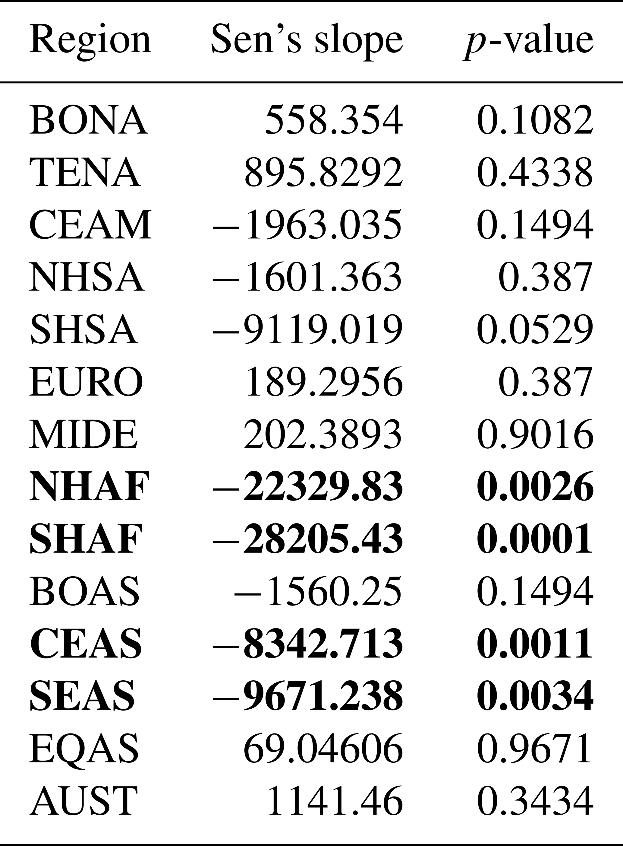
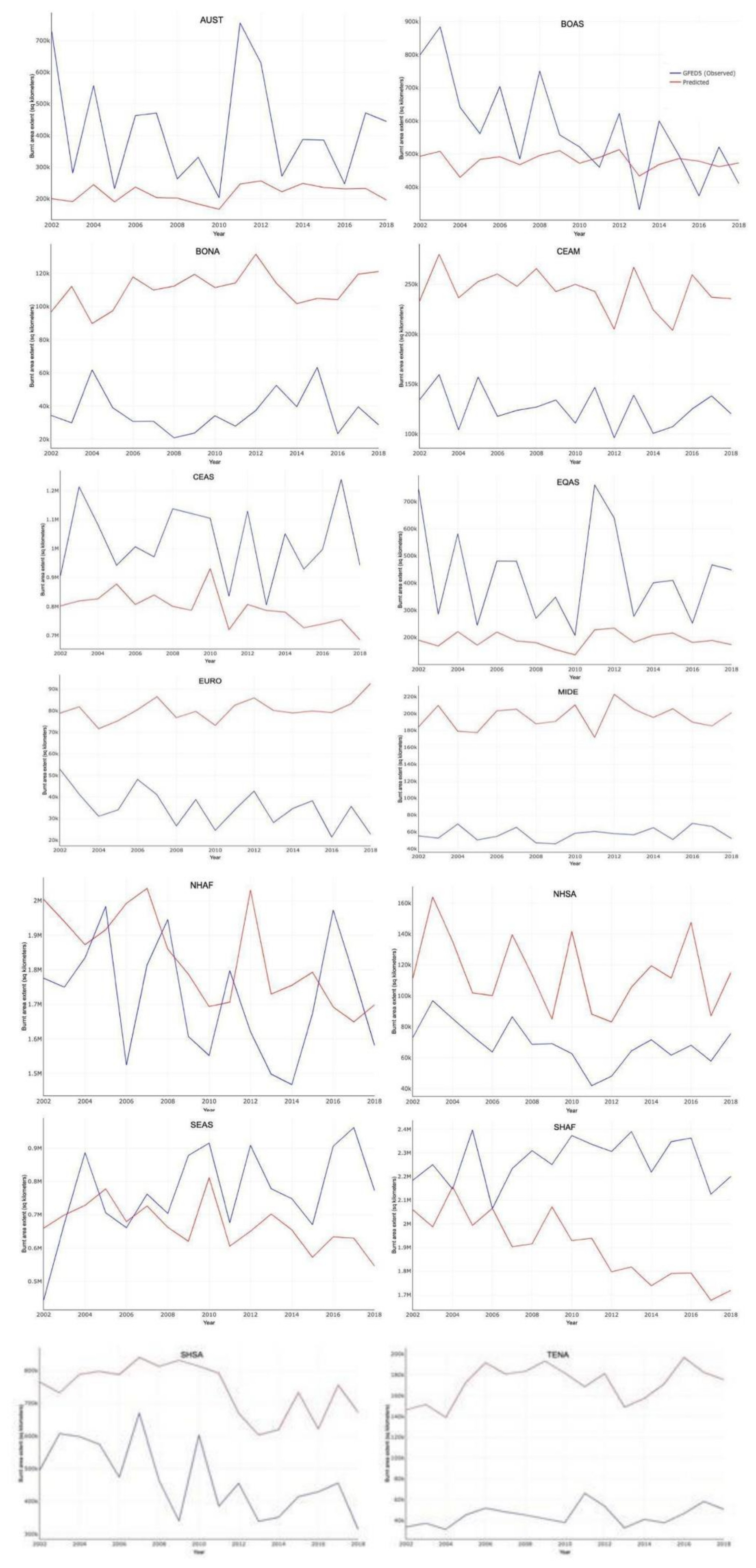
Figure A1 Shows the observed (in red) and predicted (in blue) interannual variability in burnt area fractions across different GFED regions.

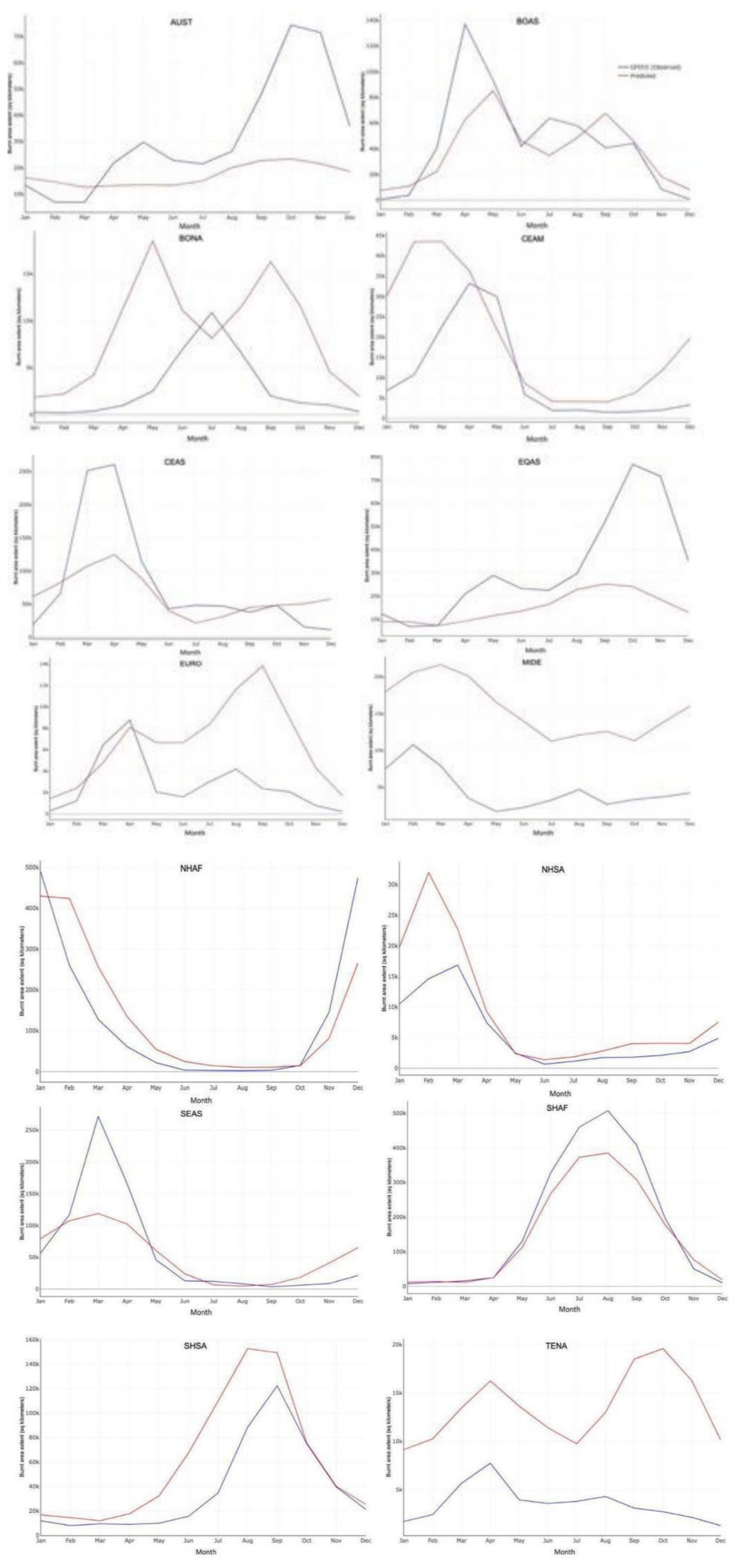
Figure A2 Shows the observed (in red) and predicted (in blue) seasonal variability in burnt area fractions across different GFED regions.

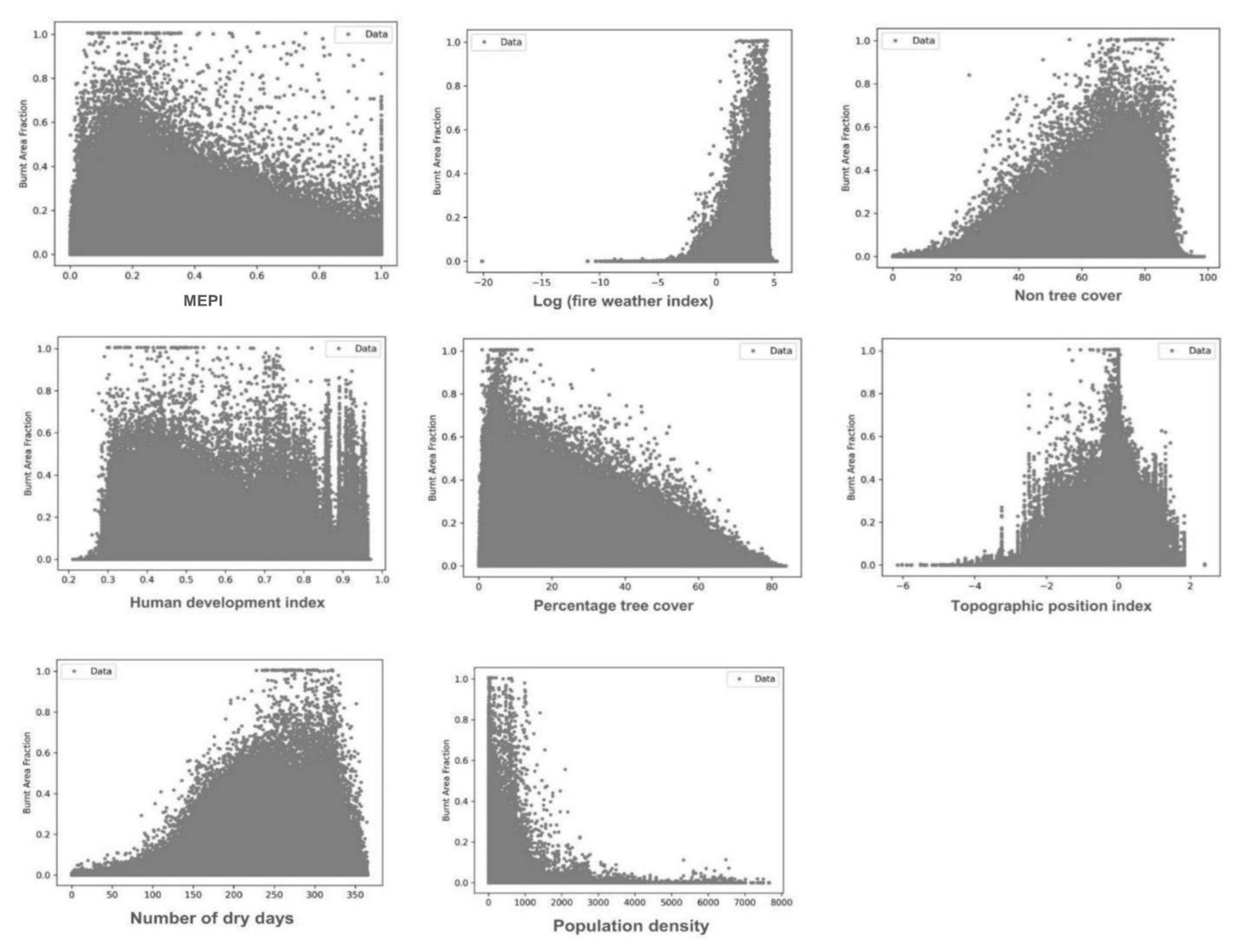
Figure A3 Scatter plots illustrating single-factor relationships between burnt area fraction and various environmental and socio-economic variables: Monthly Ecosystem Productivity Index, Fire Weather Index, Percentage Non-Tree Cover, Human Development Index, Percentage Tree Cover, Topographic Position Index, Percentage Dry Days, Road Density, Precipitation Seasonality and Annual Precipitation Index. The plots highlight distinct patterns, such as the negative correlation between percentage tree cover and burnt area fraction, and the positive correlation between number of dry days and burnt area fraction.

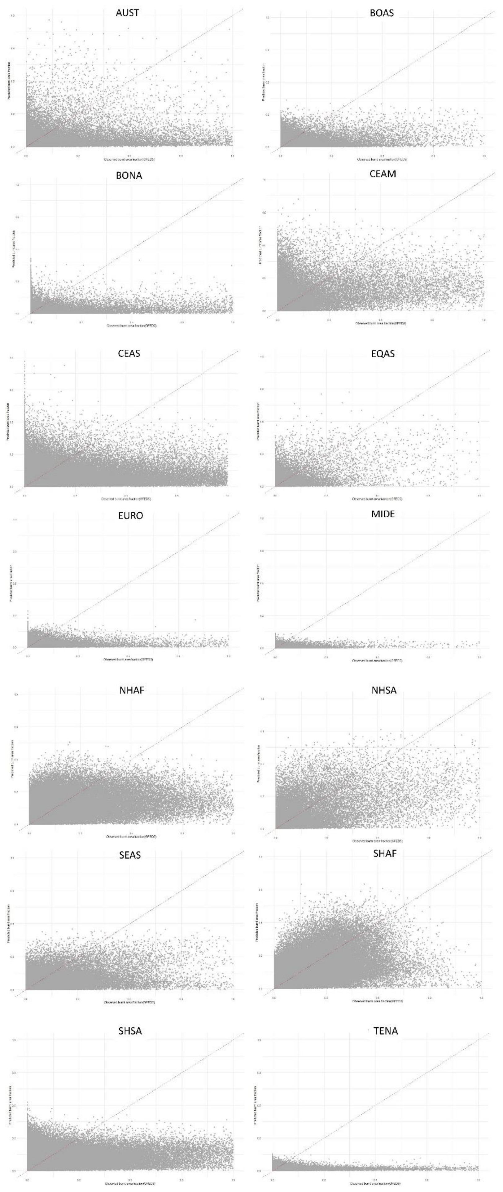
Figure A4 Scatter plots illustrating interannual comparison by GFED regional boundaries between observed burnt area fraction (GFED5) and predicted burnt area fraction for the period between 2002 and 2018.

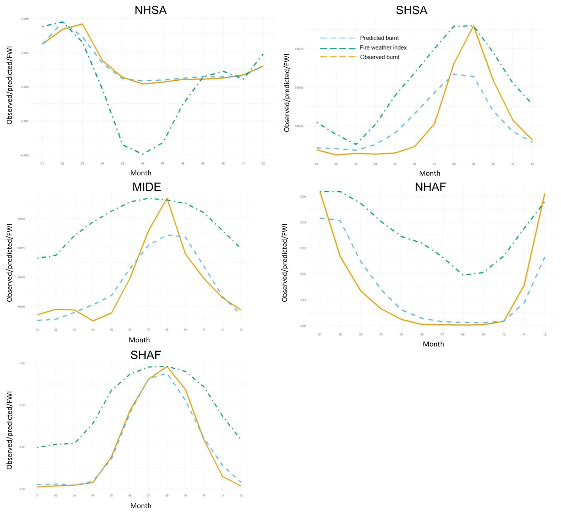
Figure A5 Shows the seasonal comparison by GFED5 regional boundaries between observed burnt area (in orange), predicted burnt (in sky blue), fire weather index (in bluish green).