Biological production in the Indian Ocean upwelling zones –Part 1: refined estimation via the use of a variable compensation depth in ocean carbon models

Biological modelling approach adopted by the Ocean Carbon-Cycle Model Intercomparison Project (OCMIP-II) provided amazingly simple but surprisingly accurate rendition of the annual mean carbon cycle for the global ocean. Nonetheless, OCMIP models are known to have seasonal biases which are typically attributed to their bulk parameterisation of compensation depth. Utilising the criteria of surface Chl a-based attenuation of solar radiation and the minimum solar radiation required for production, we have proposed a new parameterisation for a spatially and temporally varying compensation depth which captures the seasonality in the production zone reasonably well. This new parameterisation is shown to improve the seasonality of CO₂ fluxes, surface ocean pCO₂, biological export and new production in the major upwelling zones of the Indian Ocean. The seasonally varying compensation depth enriches the nutrient concentration in the upper ocean yielding more faithful biological exports which in turn leads to accurate seasonality in the carbon cycle. The export production strengthens by ∼ 70 % over the western Arabian Sea during the monsoon period and achieves a good balance between export and new production in the model. This underscores the importance of having a seasonal balance in the model export and new productions for a better representation of the seasonality of the carbon cycle over upwelling regions. The study also implies that both the biological and solubility pumps play an important role in the Indian Ocean upwelling zones.

1 Introduction

The Indian Ocean is characterised by the unique seasonally reversing monsoon wind systems which act as the major physical drivers for the coastal and open-ocean upwelling processes. The major upwelling systems in the Indian Ocean are (1) the western Arabian Sea (WAS; Ryther and Menzel, 1965; Smith, 2001; Sarma, 2004; Wiggert et al., 2005, 2006; Murtugudde et al., 2007; McCreary et al., 2009; Naqvi et al., 2010; Prasanna Kumar et al., 2010; Roxy et al., 2015), (2) the Sri Lanka Dome (SLD; Vinayachandran and Yamagata, 2008; Vinayachandran et al., 2004), (3) the Java and Sumatra coasts (SC; Murtugudde et al., 1999; Susanto et al., 2001; Osawa and Julimantoro, 2010; Xing et al., 2012) and (4) the Seychelles–Chagos thermocline ridge (SCTR; Murtugudde and Busalacchi, 1999; Dilmahamod et al., 2016, Fig. 1). The physical and biological processes and their variability over these key regions are inseparably tied to the strength of the monsoon winds and associated nutrient dynamics. The production and its variability over these coastal upwelling systems are a key concern for the fishing community, since they affect the day-to-day livelihood of the coastal populations (Harvell et al., 1999; Roxy et al., 2015; Praveen et al., 2016) and are important for the Indian Ocean rim countries due to their developing country status.

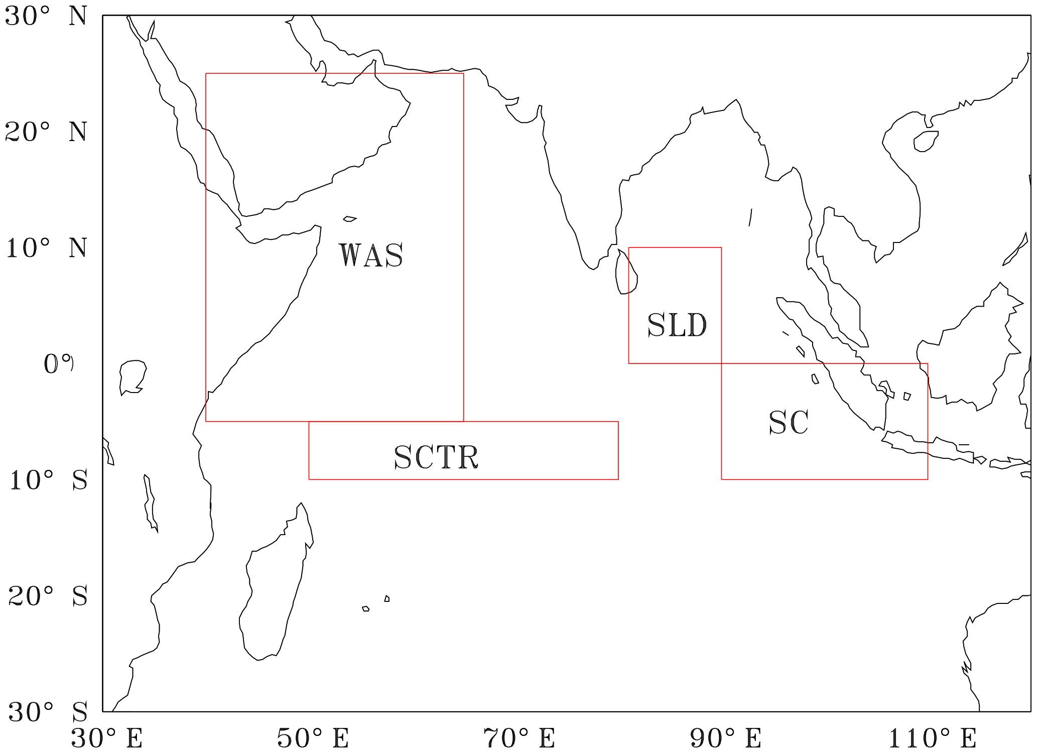
Figure 1 Red boxes shows the study regions (1) WAS (western Arabian Sea, 40–65^∘ E, 5^∘ S–25^∘ N), (2) SLD (Sri Lanka Dome, 81–90^∘ E, 0–10^∘ N), (3) SC (Sumatra coast, 90–110^∘ E, 0–10^∘ S) and (4) SCTR (Seychelles–Chagos thermocline ridge, 50–80^∘ E, 5–10^∘ S).

The Arabian Sea is a highly productive coastal upwelling system characterised by phytoplankton blooms both in summer (Prasanna Kumar et al., 2001; Naqvi et al., 2003; Wiggert et al., 2005) and winter (Banse and McClain, 1986; Wiggert et al., 2000; Barber et al., 2001; Prasanna Kumar et al., 2001; Sarma, 2004). The Arabian Sea is known for having the second largest Tuna fishing region in the Indian Ocean (Lee et al., 2005). The Somali and Omani upwelling regions experience phytoplankton blooms that are prominent, with net primary production (NPP) exceeding 435 g C m⁻² yr⁻¹ (Liao et al., 2016). On the other hand productivity over the SLD (Vinayachandran and Yamagata, 1998) is triggered by open-ocean Ekman suction with strong Chl a blooms during the summer monsoon (Murtugudde et al., 1999; Vinayachandran et al., 2004). Similarly, the SC upwelling is basically due to the strong alongshore winds, and its variation is associated with the impact of equatorial and coastal Kelvin waves (Murtugudde et al., 2000; Valsala and Rao, 2016). The interannual variability associated with the Java–Sumatra coastal upwelling is strongly coupled with ENSO (El Niño–Southern Oscillation) through the Walker cell and Indonesian throughflow (Susanto et al., 2001; Valsala et al., 2011) and peaks from July to August with a potential new production of 0.1 Pg C yr⁻¹ (Xing et al., 2012). The SCTR productivity has a large spatial and interannual variability. The warmer upper-ocean condition associated with El Niño reduces the amplitude of subseasonal SST variability over the SCTR (Jung and Kirtman., 2016). The Chl a concentration peaks in summer when the south-east trade winds induce mixing and initiate the upwelling of nutrient-rich water (Murtugudde et al., 1999; Wiggert et al., 2006; Vialard et al., 2009; Dilmahamod et al., 2016).

Understanding the biological production and variability in the upwelling systems is important because it gives us crucial information regarding marine ecosystem variability (Colwell, 1996; Harvell et al., 1999). The observations also provide vital insights into physical and biological interactions of the ecosystem (Naqvi et al., 2010) as well as the biophysical feedbacks (Murtugudde et al., 1999), although limitations of sparse observations often force us to depend on models to examine the large spatio-temporal variability of the ecosystem (Valsala and Maksyutov, 2013). Simple- to intermediate-complexity marine ecosystem models have been employed in several of the previous studies (Sarmiento et al., 2000; Orr et al., 2001; Matsumoto et al., 2008). However, the representation of marine ecosystems with proper parameterisations in models has always been a daunting task. This is an impediment to the accurate representation of biological primary and export productions in models (Friedrichs et al., 2006, 2007) and these issues also impact the modelling of upper trophic levels (Lehodey et al., 2010).

Biological production can be quantified with a better understanding of primary production, which depends on water temperature, light and nutrient availability (Brock et al., 1993; Moisan et al., 2002) and this became the key reason for parameterising production in models as one or more combinations of these terms (Yamanaka et al., 2004). Any of these basic parameters can be tweaked to alter production in models. For example, the availability of nutrients and light determines the phytoplankton growth (Eppley, 1972) or growth rate (Boyd et al., 2013). Stoichiometry and carbon-to-Chl a ratios are other important factors to be considered in modelling (Christian et al., 2001; Wang et al., 2009) but we will not consider them in this study.

The Ocean Carbon-Cycle Model Intercomparison Project (OCMIP) greatly improved our understanding of the global carbon cycle (Najjar and Orr, 1998). OCMIP-II further introduced a simple phosphate-dependent production term in biological models for long-term simulations of the carbon cycle in response to anthropogenic climate change with an accurate annual mean state (Najjar and Orr, 1998; Orr et al., 2001; Doney et al., 2004). However, the OCMIP-II model simulations come with a penalty of strong seasonal biases when compared with the observations (Orr et al., 2003). In this protocol, the community compensation depth (hereafter Zc) is defined as the depth at which photosynthesis equals the entire community respiration, and the irradiance at which this balance achieved is the compensation irradiance (E_com). Note that Zc is clearly different from the conventional euphotic zone depth (Morel, 1988). Within Zc, the production of organic phosphorous representing the biological production (in the present context the net community production; NCP) is given as $J_{\mathrm{prod}}=\frac{\mathrm{1}}{\mathit{\tau }}\left(\left[{\mathrm{PO}}_{\mathrm{4}}\right]-\left[{\mathrm{PO}}_{\mathrm{4}}{}^{\ast }\right]\right)$, where [PO₄] is the model phosphate concentration and [PO₄^∗] is observational phosphate concentration. τ is the restoration timescale, assumed to be 30 days. Whenever the model phosphate exceeds the observational phosphate, it allows production. At Zc, the NCP is zero and above Zc the net primary production (NPP) exceeds the community respiration and the ecosystem will grow (Smetacek and Passow, 1990; Gattuso et al., 2006; Sarmiento and Gruber, 2006; Regaudix-de-Gioux and Duarte, 2010; Marra et al., 2014). However, Zc was held constant in time and space in OCMIP-II models (Najjar and Orr, 1998; Matsumoto et al., 2008) because the OCMIP-II protocol takes a minimalist approach to biology and simplifies the model calculations with a very limited set of state variables suitable for long-term simulations when implemented in coarse-resolution models (Orr et al., 2005). However, in reality Zc varies in space and time (Najjar and Keeling, 1997) just as the euphotic zone depth does, as documented in ship measurements (Qasim, 1977, 1982). The variation in Zc indicates the seasonality of the production zone itself.

Most of the biophysical models prescribe a constant value for Zc, e.g. a default value of Zc = 75 m in OCMIP-II protocol (Najjar and Orr, 1998) and Zc = 100 m in the Minnesota Earth System Model (Matsumoto et al., 2008). Depending on the latitude, Zc varies between 50 and 100 m in the real world (Najjar and Keeling, 1997). In our study we have attempted a novel biological parameterisation scheme for spatially and temporally varying Zc in the OCMIP-II framework by representing production as a function of solar radiation (Parsons et al., 1984) and prescribed Chl a. In this hypothesis, a spatially and temporally varying Zc is estimated from the vertical attenuation of insolation by the surface Chl a. The depth at which the insolation reaches the compensation irradiance (chosen as 10 W m⁻²) is taken as Zc. Phosphorous is the basic currency which limits production within this varying Zc. This spatially and temporally varying Zc represents the seasonality in the production zone which is lacking in the original OCMIP-II protocol.

Regions of sustained upwelling like the eastern equatorial Pacific are well understood in terms of the role of upwelling in increasing the surface water pCO₂ to drive an outgassing of CO₂ into the atmosphere (Feely et al., 2001; Valsala et al., 2014). The Indian Ocean, on the other hand, experiences only seasonal upwelling, which is relatively weak in the deep tropics but stronger off the coasts of Somalia and Oman and in the SLD (Valsala et al., 2013). The relative importance of the solubility vs. biological pump is not well understood. Our focus here on implementing seasonality in Zc of OCMIP models nonetheless leads to new insights into the impact of improved biological production on surface water pCO₂ and air–sea CO₂ fluxes. The improvements are due to the effect of a variable Zc over the Indian Ocean, and the sensitivity experiments where upwelling is muted strongly imply that the biological pump may play as much of a role as the solubility pump in determining surface pCO₂ and CO₂ fluxes over the Indian Ocean.

The paper is organised as follows. The model, data and methods are detailed in Sect. 2. The spatially inhomogeneous Zc derived with the new parameterisation and its impact on simulated seasonality of biology and carbon cycle are detailed in Sect. 3. Further a conclusion is provided in Sect. 4.

2 Model, data and methods

2.1 Model

The study utilises the offline Ocean Tracer Transport Model (OTTM; Valsala et al., 2008) coupled with the OCMIP biogeochemistry model (Najjar and Orr, 1998). OTTM does not compute currents and stratifications (i.e. temperature and salinity) on its own. It is capable of accepting any ocean model or data-assimilated product as its physical drivers. The physical drivers prescribed include 4-dimensional currents (U, V, W), temperature, salinity and 3-dimensional mixed-layer depth, surface freshwater and heat fluxes, surface wind stress and sea surface height. The resolution of the model set-up is similar to the parent model, from which it borrows the physical drivers. With the given input of Geophysical Fluid Dynamics Laboratory (GFDL) reanalysis data (Chang et. al., 2012), the zonal and meridional resolutions are 1^∘ with 360 grid points longitudinally and 1^∘ at higher latitudes but have a finer resolution of 0.8^∘ in the tropics, with 200 latitudinal grid points. The model has 50 vertical levels with 10 m increments in the upper 225 m and stretched vertical levels below 225 m. The horizontal grids are formulated in spherical coordinates and vertical grids are in z levels. The model employs a B-grid structure in which the velocities are resolved at corners of the tracer grids. The model uses a centred-in-space and centred-in-time (CSCT) numerical scheme along with an Robert–Asselin filter (Asselin, 1972) to control the ripples in CSCT.

The tracer concentration (C) evolves with time as

$$\begin{array}{ll}{\displaystyle \frac{\partial C}{\partial t}}& {\displaystyle }+U{\mathrm{\nabla }}_{\mathrm{H}}C+W{\displaystyle \frac{\partial C}{\partial z}}={\displaystyle \frac{\partial }{\partial z}}{K}_z{\displaystyle \frac{\partial }{\partial z}}C\\ \text{(1)}& {\displaystyle }& {\displaystyle }+{\mathrm{\nabla }}_{\mathrm{H}}\left(K_h{\mathrm{\nabla }}_{\mathrm{H}}C\right)+J+F,\end{array}$$

where ∇_H is the horizontal gradient operator, U and W are the horizontal and vertical velocities. K_z is the vertical mixing coefficient, and K_h is the two-dimensional diffusion tensor. J represents any sink or source due to the internal consumption or production of the tracer. F represents the emission or absorption of fluxes at the ocean surface. Here, the source and sink terms are provided through the biogeochemical model. Vertical mixing is resolved in the model using K-profile parameterisation (KPP; Large et al., 1994).

In addition to KPP, the model uses a background vertical diffusion reported by Bryan and Lewis (Bryan and Lewis, 1979). For horizontal mixing, the model incorporates Redi fluxes (Redi, 1982) and GM fluxes (Gent and McWilliams, 1990), which represent the eddy-induced variance in the mean tracer transport. A weak Laplacian diffusion is also included in the model for computational stability where the sharp gradient in concentration occurs.

2.2 Biogeochemical model

The biogeochemical model used in the study is based on the OCMIP-II protocol as stated above. The main motivation of the OCMIP-II protocol is to employ a minimalist approach to simulate the ocean carbon cycle with a nutrient restoration approach to calculate the oceanic biological production (Najjar et al., 1992; Anderson and Sarmiento, 1995). The present version of the model has four prognostic variables coupled with the circulation field, viz. inorganic phosphorus (PO₄³⁻), dissolved organic phosphorus (DOP), dissolved inorganic carbon (DIC) and alkalinity (ALK). The basic currency for the biological model is phosphorous because of the availability of a more extensive phosphate database and to eliminate the complexities associated with nitrogen fixation and denitrification. Detailed model equations and variables are provided in Appendix A with only a brief description given below.

The production of organic phosphorus in the model using the nutrient restoring approach is given by

$$\begin{array}{ll}{\displaystyle }{J}_{\mathrm{prod}}=& {\displaystyle }{\displaystyle \frac{\mathrm{1}}{\mathit{\tau }}}(\left[{\mathrm{PO}}_{\mathrm{4}}\right]-[{\mathrm{PO}}_{\mathrm{4}}\left]{}^{\ast }\right)\\ \text{(2)}& {\displaystyle }& {\displaystyle }\left[{\mathrm{PO}}_{\mathrm{4}}\right]\mathit{>}[{\mathrm{PO}}_{\mathrm{4}}{]}^{\ast };Z\mathit{<}Zc\end{array}$$

$$\begin{array}{}\text{(3)}& {\displaystyle }{J}_{\mathrm{prod}}=\mathrm{0},\left[{\mathrm{PO}}_{\mathrm{4}}\right]\le [{\mathrm{PO}}_{\mathrm{4}}{]}^{\ast },\end{array}$$

where J_prod represents the biogeochemical flows with respect to production of organic phosphorous. [PO₄]^∗ is the observed phosphate concentration and τ= 30 days is the restoration timescale (Najjar et. al., 1992). The conversion of phosphorus to carbon is done by multiplying the Redfield ratio ($R_{\mathrm{C}:\mathrm{P}}=$ 117).

The vertically integrated new production (g C m⁻² yr⁻¹) in the model is defined as

$$\begin{array}{}\text{(4)}& \mathrm{new}\mathrm{production}=\underset{zc}{\overset{\mathrm{0}}{\int }}-J_{\mathrm{prod}}\mathrm{d}z.\end{array}$$

The export production (g C m⁻² yr⁻¹) in the model is calculated as

$$\begin{array}{}\text{(5)}& {\displaystyle }\mathrm{export}\mathrm{production}=(\mathrm{1}-\mathit{\sigma })\underset{\mathrm{0}}{\overset{zc}{\int }}{J}_{\mathrm{prod}}\mathrm{d}z.\end{array}$$

Air–sea CO₂ flux in the model is estimated by

$$\begin{array}{}\text{(6)}& F=K_w\mathrm{\Delta }p{\mathrm{CO}}_{\mathrm{2}},\end{array}$$

where K_w is gas transfer velocity and pCO₂ is the difference in partial pressure of carbon dioxide between the ocean and atmosphere.

pCO₂ is calculated in the model by using DIC and ALK and is given by

$$\begin{array}{}\text{(7)}& {\displaystyle }p{\mathrm{CO}}_{\mathrm{2}}={\displaystyle \frac{\left[\mathrm{DIC}\right]}{K_{\mathrm{0}}}}{\displaystyle \frac{[H^{+}{]}^{\mathrm{2}}}{{\left[H^{+}\right]}^{\mathrm{2}}+K_{\mathrm{1}}\left[H^{+}\right]+K_{\mathrm{1}}{K}_{\mathrm{2}}}},\end{array}$$

where [H⁺] is calculated using the Newton–Raphson iterative method (Press et al., 1996; Najjar and Orr, 1998). K₀ is the solubility constant of CO₂, and K₁ and K₂ are the dissociation constants for carbonic acid (Sarmiento and Gruber, 2006; Mehrbach et al., 1973; Weiss, 1974; Dickson and Millero, 1987; Najjar and Orr, 1998).

Details of all parameters in the biogeochemical model and calculations of solubility and biological pump are listed in Appendix A. The design and validation of the physical model is reported by Valsala et al. (2008), Valsala and Maksyutov (2010b) and the biogeochemical model by Najjar and Orr (1998).

2.3 Data

To validate the model results, observational data sets of CO₂ flux and pCO₂ are taken from Takahashi et al. (2009). Satellite-derived NPP data were taken from a Sea-viewing Wide Field-of-view Sensor (SeaWiFS) Chl a product, calculated using a Vertically Generalized Production Model (VGPM; Behrenfeld and Falkowski, 1997). The NPP data are scaled to export production (EP) by being multiplied with an e ratio (e = 0.37), representative of Indian Ocean upwelling zones (Sarmiento and Gruber, 2006; Laws et al., 2000; Falkowski et al., 2003). The initial conditions for PO₄ are taken from the World Ocean Atlas (Garcia et al., 2014). Initial conditions for DIC and ALK are taken from the Global Ocean Data Analysis Project (GLODAP; Key et al., 2004) data set. The dissolved organic phosphorous (DOP) is initialised with a constant value of 0.02 µ mol kg⁻¹ (Najjar and Orr, 1998). The data sources and citations are provided in the “Data availability” section.

2.4 Methods

A spin-up for 50 years from the given initial conditions is performed with the climatological physical drivers. As the initial conditions are provided from a mean state of observed climatology, this duration of spin-up is sufficient to reach statistical equilibrium in the upper 1000 m (Le Quere et al., 2000). Atmospheric pCO₂ has been set to a value from the 1950s in the spin-up run for calculating the air–sea CO₂ exchange. A seasonal cycle of atmospheric pCO₂ has been prescribed as in Keeling et al. (1995).

After the spin-up, an interannual simulation for 50 years from 1961 to 2010 has been carried out with the corresponding observed atmospheric pCO₂ described in Keeling et al. (1995). The first 5 years of the interannual run were looped five times through the physical fields of 1961 repeatedly for a smooth merging of the spin-up restart to the interannual physical variables. Since the study is focused on bias corrections to the seasonal cycle of pCO₂ and DIC with a variable Zc, a model climatology for the carbon cycle has been constructed from 1990 to 2010, which includes the anthropogenic increase of oceanic DIC in the climatological calculation and is comparable with the Takahashi et al. (2009) observations.

An additional two sensitivity experiments were performed separately by providing annual mean currents or temperatures as drivers over selected regions of the basin in order to segregate the role of varying Zc in improving the seasonality of the carbon cycle. The aim of these sensitivity experiments is to understand how successful the new parameterisation for Zc is in capturing the carbon cycle variability related to the upwelling episodes even though the seasonal cycle in physics is suppressed. The model driven with annual mean currents suppresses the effect of the upwelling by muting the Ekman divergence over the region of interest. On the other hand, the model forced with annual mean temperatures suppresses the cooling effect of upwelling. A smoothing technique with linear interpolation $(U=U\left(\mathrm{1}-x\right)+\overline{U}x)$ is applied to the offline data in order to blend the annual mean fields ($\overline{U})$ provided to the selected region with the rest of the domain (U) in order to reduce a sudden transition at the boundaries. Here x represents an index which varies between 0 and 1 within a distance of 10^∘ from the boundaries of the region of interest to the rest of the model domain. Results of the sensitivity experiments are provided in the Supplement.

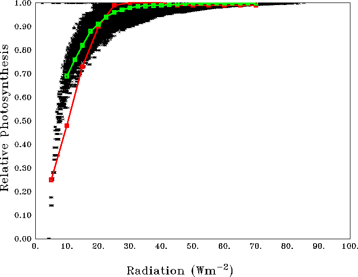
Figure 2 Scatter of average relative photosynthesis versus different light intensities in the model (black dots) and its mean (green curve). The red curve shows the theoretical P–I curve from Parsons et al. (1984).

2.5 Community compensation depth (Zc) parameterisation

The OCMIP-II protocol separates the production and consumption zones by a depth termed compensation depth (Zc); the depth at which photosynthesis is large enough to balance the community respiration (i.e. both the autotrophic and heterotrophic respiration). At the community compensation depth, the NCP is zero, i.e. NCP = NPP–R_h= 0 (i.e. NPP = GPP–R_a), GPP is gross primary production, and R_h and R_a are the heterotrophic and autotrophic respirations, respectively (Smetacek and Passow, 1990; Najjar and Orr, 1998; Gattuso et al., 2006; Regaudix-de-Gioux and Duarte, 2010; Marra et al., 2014). The light intensity at Zc is compensation irradiance (E_com), the irradiance at which the gross community primary production balances respiratory carbon losses for the entire community (Gattuso et al., 2006; Regaudix-de-Gioux and Duarte, 2010). We define a spatially and temporally varying compensation depth (hereafter varZc) as a depth at which compensation irradiance (attenuated by surface Chl a, Jerlov, 1976) reaches a minimum value of 10 W m⁻². In this way, the varZc has both spatio-temporal variability of light as well as Chl a. The Chl a is given as a monthly climatology, constructed from satellite data. Observations show that the primary production reduces rapidly to 20 % or less of the surface value below a threshold of 10 W m⁻² (Parsons et al., 1984; Ryther, 1956; Sarmiento and Gruber, 2006). Moreover higher ocean temperatures (those in the tropics) enhance the respiration rates, resulting in high compensation irradiance (Ryther, 1956; Parsons et al., 1984; Lopez-Urrutia et al., 2006; Regaudix-de-Gioux and Duarte, 2010). A study by Regaudix-de-Gioux and Duarte (2010) reported the mean value of compensation irradiance over the Arabian Sea as 0.4 ± 0.2 mol photon m⁻² day⁻¹, which is close to 10 W m⁻² day⁻¹.

Figure 2 compares the scatter of average relative photosynthesis (See Appendix B for details) within varZc as a function of solar radiation for the Indian Ocean. This encapsulates the corresponding curve from the observations for the major phytoplankton species in the ocean such as diatoms, green algae and dinoflagellates (Ryther et al., 1956; Parsons et al., 1984; Sarmiento and Gruber, 2006). The model permits 100 % production of organic phosphorus for radiation above 10 W m⁻². However the availability of phosphate concentration in the model acts as an additional limit for production, which indirectly represents the photoinhibition at higher irradiance, for example in the oligotrophic gyres.

3 Results and discussions

The inclusion of seasonality in Zc by way of parameterising varZc leads to a remarkable spatio-temporal variability in Zc (Fig. 3). Zc over the Arabian Sea varies from 10 to 25 m during December to February (DJF) and deepens to 45 m during March to May (MAM) due to the increase in the surface solar radiation. During the monsoon season, i.e. June to September (JJAS), Zc again shoals to 10–35 m due to the attenuation of solar radiation by the increased biological production (Chl a). During October to November (ON), Zc slightly deepens compared to JJAS.

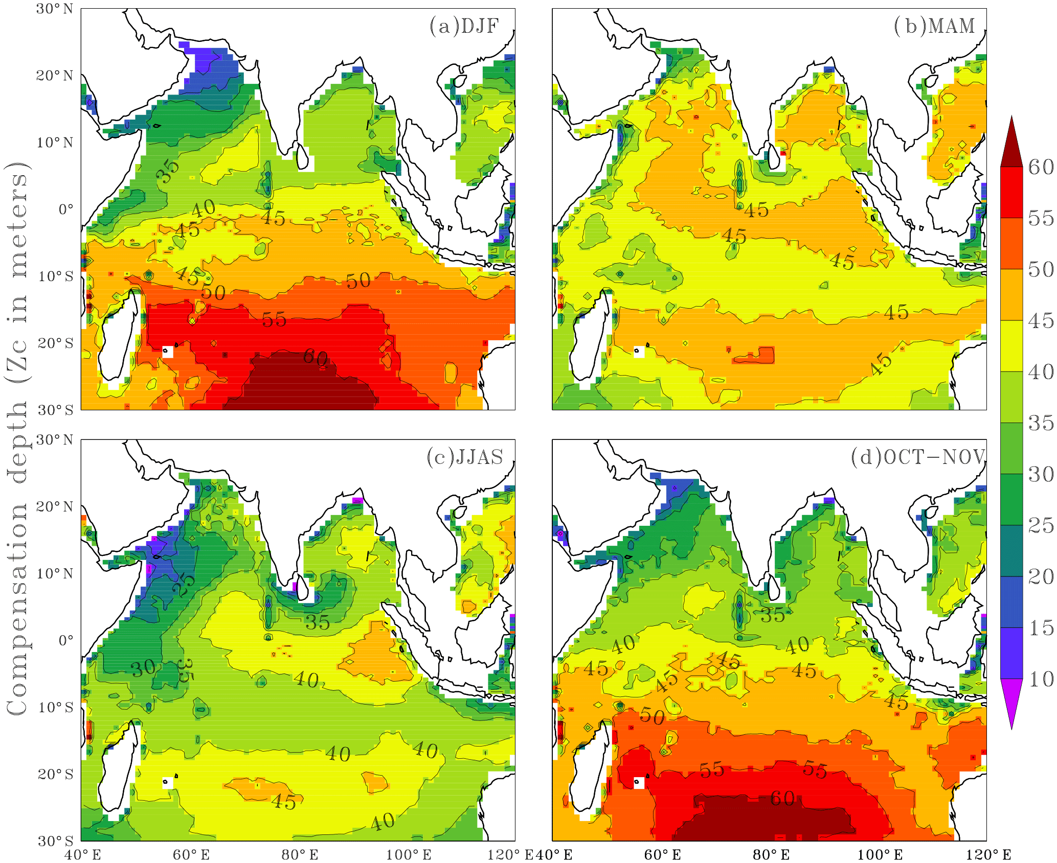
Figure 3 Seasonal mean maps of varying compensation depth (varZc), (a) December to February (DJF), (b) March to May (MAM), (c) June to September (JJAS) and (d) October to November (ON). Units are metres.

The Bay of Bengal Zc deepens from 35 to 40 m during DJF and further deepens to 50 m during MAM when the solar radiation is maximum and biological production is minimum (Prasanna Kumar et al., 2002). Further reduction of Zc can be seen through JJAS as a result of a reduction in solar radiation during monsoon cloud cover. Zc during ON is 35 m on average.

The equatorial Indian Ocean can be seen as a belt of 40–45 m Zc throughout the season except for JJAS. During JJAS, a shallow Zc is seen near the coastal Arabian Sea (around 10 to 35 m) presumably due to the coastal Chl a blooms. Deep Zc off the coast of Sumatra (∼ 40 to 50 m) is found during JJAS. Java–Sumatra coastal upwelling is centred on SON (Susanto et al., 2001) and upwelling originates at around 100 m depth (Valsala and Maksyutov, 2010a; Xing et al., 2012).

Southward of 10^∘ S in the oligotrophic gyre region, Zc varies from 40 m to more than 60 m throughout the year. A conspicuous feature observed while parameterising the solar radiation and Chl a-dependent Zc is that its maximum value never crosses 75 m, especially in the Indian Ocean which is the value specified in OCMIP-II models. The cut-off depth of 75 m in OCMIP-II is obtained from observing the seasonal variance in oxygen data (Najjar and Keeling, 1997) as an indicator of the production zone. However, our results show that parameterising a production zone based on solar radiation and Chl a predicts a production zone and its variability that is largely less than 75 m. The relevance of varZc in the seasonality of the modelled carbon cycle is illustrated as follows.

3.1 Simulated seasonal cycle of pCO₂ and CO₂ fluxes

The annual mean biases in simulated CO₂ fluxes and pCO₂ were evaluated by comparing with the Takahashi et al. (2009) observations (Fig. 4). The model biases are significantly reduced with the implementation of varZc compared to that of the constant Zc (hereinafter constZc). A notable reduction in pCO₂ bias (by ∼ 10 µatm) is observed along the WAS (Fig. 4d).

In order to address the role of the new biological parameterisation of a variable Zc, we zoom in on four key regions where the biological production and CO₂ fluxes are prominent in the Indian Ocean with additional sensitivity experiments (see Introduction and references therein). The regions (boxes shown in Fig. 1) we considered are (1) western Arabian Sea (WAS; 40–65^∘ E, 5^∘ S–25^∘ N), (2) Sri Lanka Dome (SLD; 81–90^∘ E, 0–10^∘ N), (3) Sumatra coast (SC; 90–110^∘ E, 0–10^∘ S) and (4) Seychelles–Chagos thermocline ridge (SCTR; 50–80^∘ E, 5–10^∘ S; Fig. 1). The seasonal variations of Zc over these selected key regions are shown in Fig. 5. A detailed analysis of CO₂ fluxes, pCO₂, biological export and new productions and the impact of varZc simulations in improving the strength of biological pump and solubility pump for these key regions are presented below.

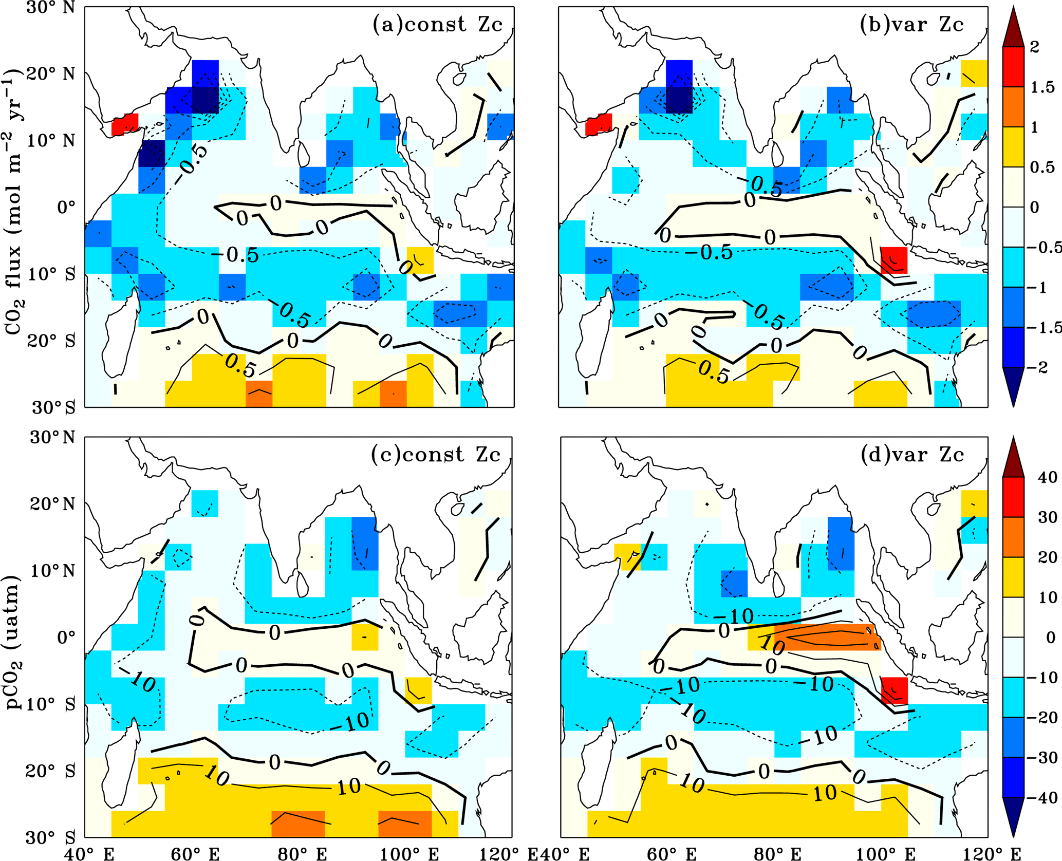
Figure 4 Annual mean biases in the model evaluated against Takahashi et al. (2009) observations for CO₂ flux (a, b) and pCO₂ (c, d) with constant Zc (constZc) and varying Zc (varZc). Units of CO₂ flux and pCO₂ are mol m⁻² yr⁻¹ and µatm, respectively.

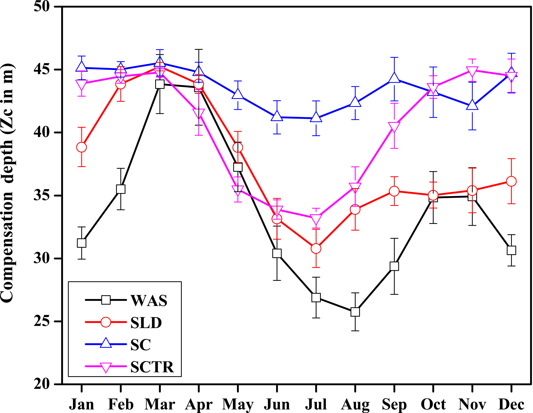
Figure 5 Seasonal variations in varZc over the study regions shown as climatology computed over 1990–2010. Error bar shows standard deviations of individual months over these years. Units are metres.

3.2 Western Arabian Sea (WAS)

The WAS Zc has a double peak pattern over the annual cycle. During the February–March period, Zc deepens to a maximum of 43.85 ± 2.3 m into March and then shoals to 25.75 ± 1.5 m (Fig. 5) during the monsoon period (uncertainty represents the interannual standard deviations of monthly data from 1990 to 2010). This shoaling of Zc depth during the monsoon indicates the potential ability of the present biological parameterisation to capture the wind-driven upwelling related production in the WAS. During the post-monsoon period, the second deepening of Zc occurs during November with a maximum depth of 34.91 ± 2.2 m. The ability to represent the seasonality of the production zone renders a unique improvement in CO₂ flux variability, especially in the WAS in comparison to the OCMIP-II experiments (Orr et al, 2003; Fig. 6a).

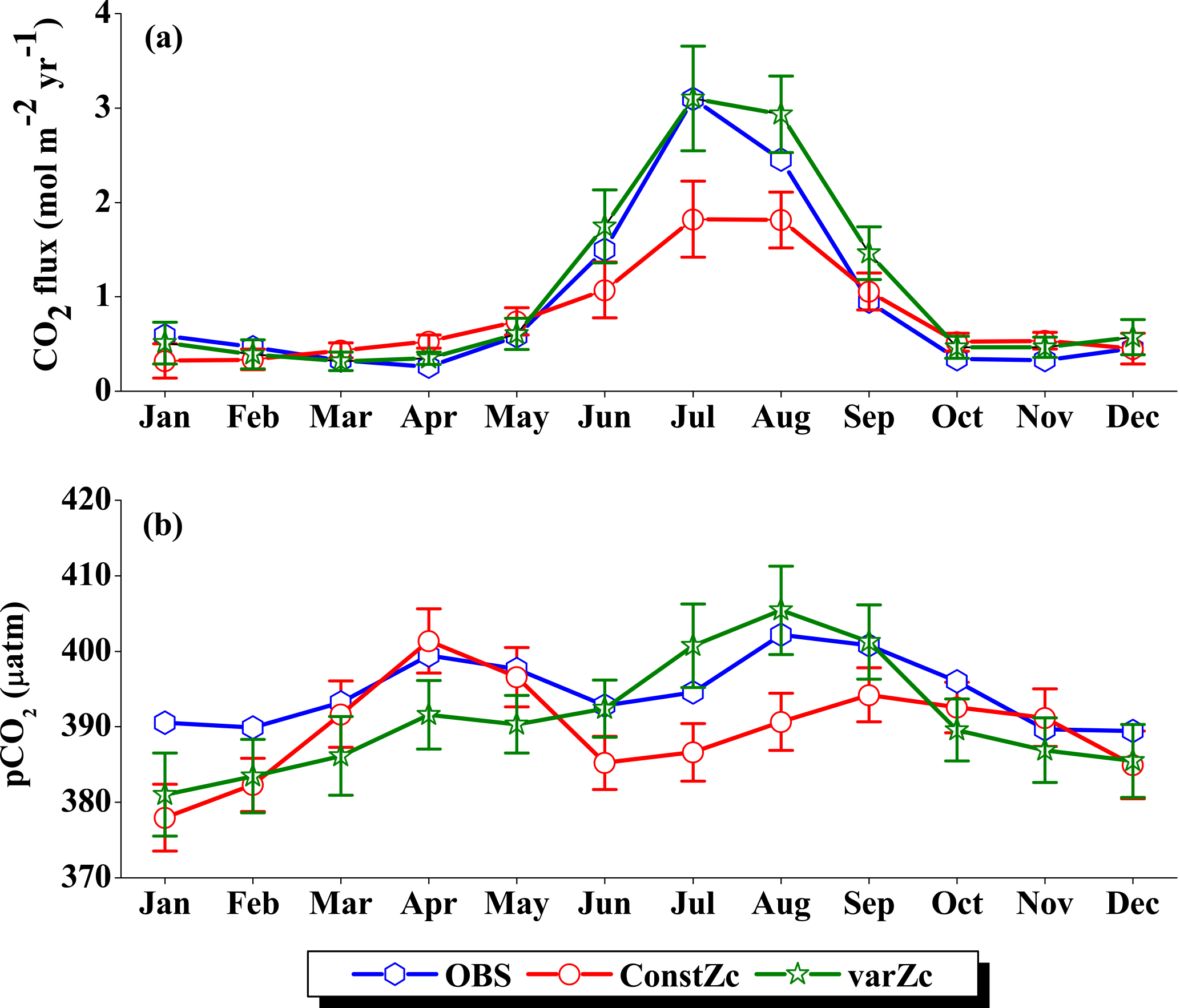
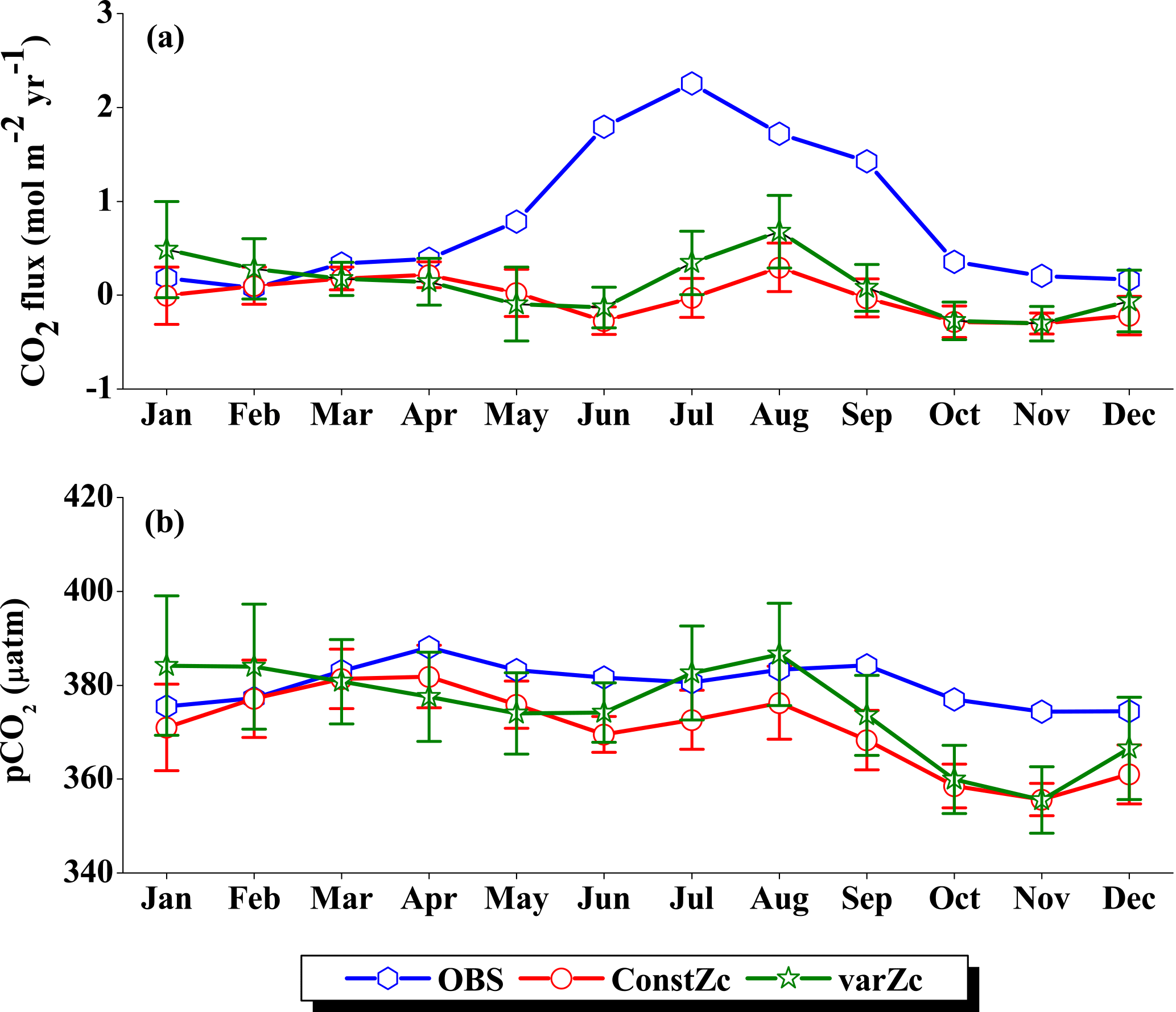
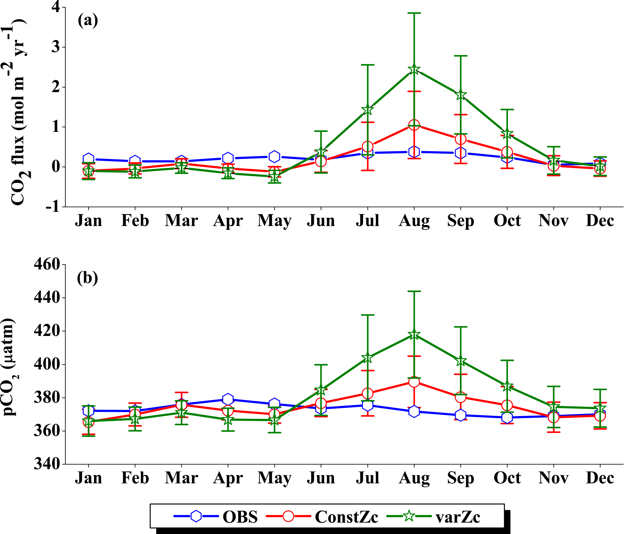
Figure 6 Comparison of model (a) CO₂ flux and (b) pCO₂ simulated with constZc and varZc with that of Takahashi et al. (2009) observations (OBS) over WAS as climatology computed over 1990–2010. Error bar shows standard deviations of individual months over these years. Units of CO₂ flux and pCO₂ are mol m⁻² yr⁻¹ and µatm, respectively. Legend is common for both graphs.

OCMIP-II simulations with a constZc of 75 m underestimate the CO₂ flux when compared to the observations of Takahashi et al. (2009). This underestimation is clearly visible during the monsoon period. Our simulations with the varZc result in better seasonality of CO₂ flux when compared with the Takahashi et al. (2009) observations (Fig. 6a). The improvement due to the varZc scheme is able to represent the seasonality of CO₂ flux better, especially during the monsoon period when wind-driven upwelling is dominant. Obviously, the relative role of the biological and solubility pumps have to be deciphered in this context.

The CO₂ fluxes during July from the observations, constZc, and varZc simulations are 3.09, 1.82 ± 0.4 and 3.10 ± 0.5 mol m⁻² yr⁻¹, respectively. South-westerly wind-driven upwelling over the WAS, especially off the Somali coast (Smith and Codispoti, 1980; Schott, 1983; Smith, 1984) and Oman (Bruce, 1974; Smith and Bottero, 1977; Swallow, 1984; Bauer et al., 1991), pulls nutrient-rich subsurface waters closer to the surface while the available turbulent energy due to the strong winds lead to mixed-layer entrainment of the nutrients, resulting in a strong surface phytoplankton bloom (Krey and Babenerd, 1976; Banse, 1987; Bauer, 1991; Brock et al., 1991). This regional bloom extends over 700 km offshore from the Omani coast due to upward Ekman pumping driven by strong, positive wind-stress curl to the north-west of the low-level jet axis and the offshore advection (Bauer et al., 1991; Brock et al., 1991, 1992; Brock and McClain, 1992; Murtugudde and Busalacchi, 1999; Valsala, 2009), resulting in strong outgassing of CO₂ flux and an enhanced pCO₂ in the WAS (Sarma, 2002; Valsala and Maksyutov, 2013). The seasonal mean CO₂ fluxes during the south-west monsoon period (JJAS) for constZc and varZc simulations are 1.44 ± 0.2 and 2.31 ± 0.4 mol m⁻² yr⁻¹. The biological parameterisation of varZc considerably improves the average CO₂ flux during the monsoon period by 0.86 ± 0.1 mol m⁻² yr⁻¹. The annual mean CO₂ fluxes from the observations, constZc and varZc simulations are 0.94, 0.80 ± 0.17 and 1.07 ± 0.2 mol m⁻² yr⁻¹. The annual mean CO₂ flux is improved by 0.27 ± 0.05 mol m⁻² yr⁻¹.

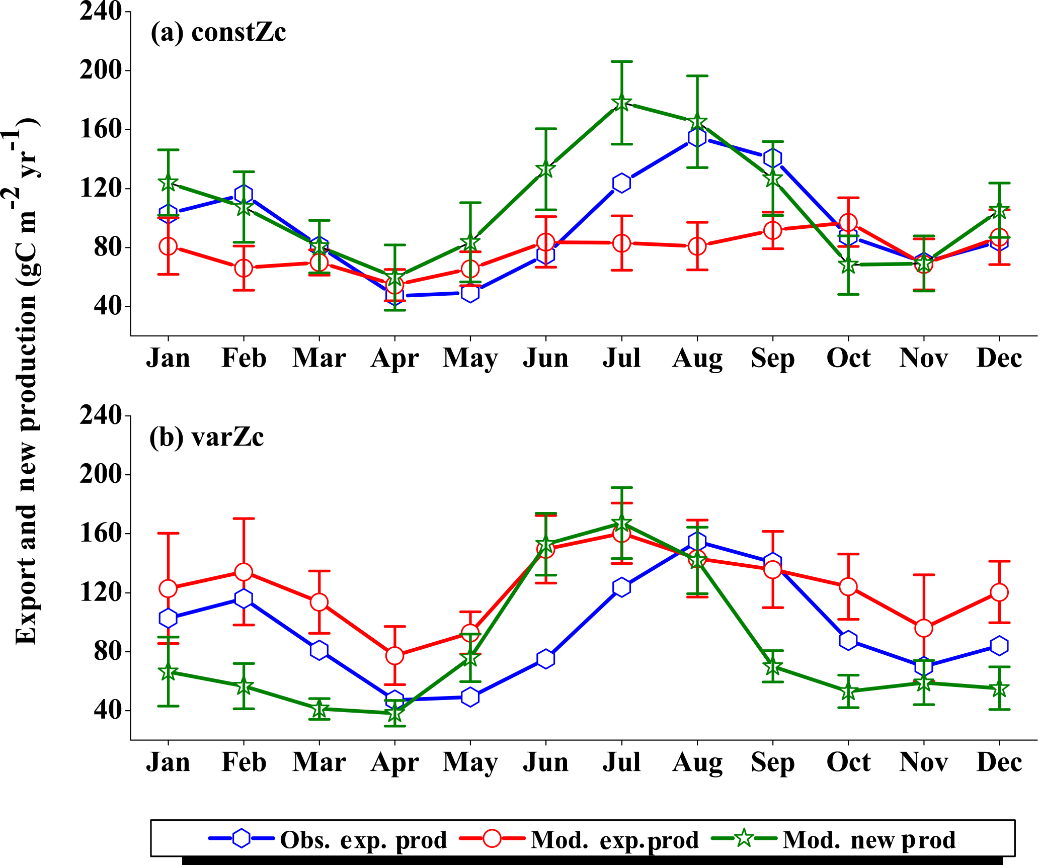
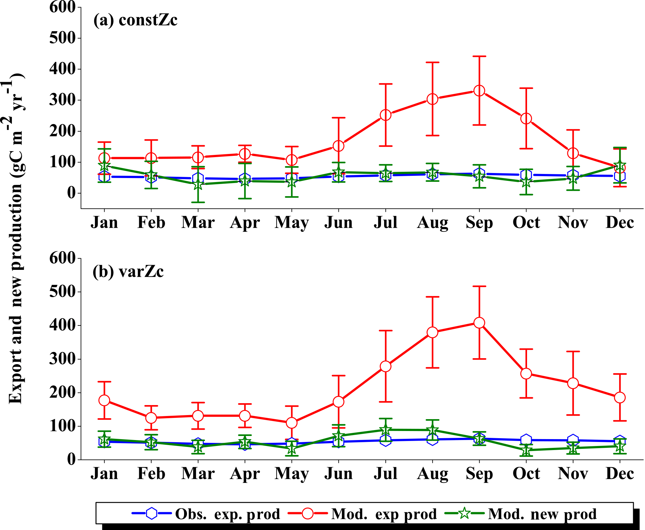
Figure 7 Comparison of model export production (Mod. exp. prod) and new production (Mod. new prod) with satellite-derived export production (Obs. exp. prod) for (a) constZc and (b) varZc simulations for WAS. Units are g C m⁻² yr⁻¹. Legends are common for both graphs.

Seasonality in pCO₂ also shows a remarkable improvement during the south-west monsoon period (Fig. 6b). The pCO₂ with constZc is considerably lower at a value of 385.22 ± 3.5 µatm during June compared to observational values of 392.83 µatm. However, varZc simulation performs better in terms of pCO₂ variability. The peak value of pCO₂ reaches up to 405.42 ± 5.8 µatm. The seasonal mean pCO₂ during the south-west monsoon period from the observations, constZc and varZc simulations are 397.58, 389.18 ± 3.6 and 399.95 ± 5.0 µatm. The improvement in pCO₂ by varZc simulation is 10.76 ± 1.3 µatm when compared with the constZc simulation. This clearly shows that constZc simulation fails to capture the pCO₂ driven by upwelling during the south-west monsoon while the varZc simulation is demonstrably better in representing this seasonal increase. The annual mean pCO₂ from the observations, constZc and varZc simulations are 394.69, 389.62 ± 3.9 and 391.19 ± 4.7 µatm. However, it is worth mentioning that there are parts of the year in which the constZc performs better compared to varZc. For instance, during MAM as well as in November, the constZc simulation yields a better comparison with the observed pCO₂, whereas varZc simulation yields a reduced magnitude of pCO₂. This may well indicate the biological vs. solubility pump controls on pCO₂ during the intermonsoons. The role of mesoscale variability in the ocean dynamics may also play a role (Valsala and Murtugudde, 2015). Nevertheless, during the most important season (JJAS) when the pCO₂, CO₂ fluxes and biological production are found to be dominant in the Arabian Sea, the varZc produces a better simulation.

The improvements shown by the use of varZc in the simulation of CO₂ flux and pCO₂ can be elicited by further analysis of the model biological production. Fig. 7 shows the comparison of model export production and new production with observational export production from satellite-derived NPP for constZc and varZc simulations. The model export production in the constZc simulation is much weaker when compared to the varZc simulation. The varZc simulation has improved the model export production. Theoretically, the new and export productions in the model should be in balance with each other (Eppley and Peterson, 1979). The constZc export production is much weaker than the new production and it is not in balance. In contrast, the varZc simulation yields a close balance among them.

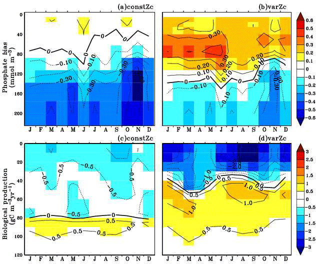
Figure 8 Annual mean bias of model phosphate when compared with climatological observational data (a) for constZc and (b) for varZc simulations. Corresponding annual mean biological source–sink profiles (c, d) in the model for WAS. Unit of phosphate is mmol m⁻³ and biological source–sink is g C m⁻³ yr⁻¹.

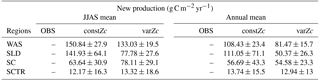
Compared with the observational export production which peaks in August at a value of 154.78 g C m⁻² yr⁻¹, the varZc-simulated export and new productions peak at values of 160.44 ± 20.4 and 167.18 ± 24.0 g C m⁻² yr⁻¹, respectively, but in July. A similar peak can be observed in constZc-simulated new production as well, with a value of 178.19 ± 28.0 g C m⁻² yr⁻¹. This apparent shift of 1 month during JJAS in the model export production as well as in the new production is noted as a caveat in the present set-up which will need further investigation. Arabian Sea production is not just limited by nutrients but also by the dust input (Wiggert et al., 2006). The dust-induced primary production in the WAS, especially over the Oman coast, is noted during August (Liao et al., 2016). The mesoscale variability in the circulation and its impact on production and carbon cycle are also limiting factors in this model as noted above.

The seasonal mean export production during the south-west monsoon period from the satellite-derived estimate is 123.57 g C m⁻² yr⁻¹, whereas for the constZc and varZc simulations it is 84.81 ± 16.0 and 147.19 ± 23.8 g C m⁻² yr⁻¹. The new biological parameterisation strengthens the model export production by 62.38 ± 7.8 g C m⁻² yr⁻¹ for the south-west monsoon period, which is over a 70 % increase. This indicates a considerable impact of the biological pump in the model-simulated CO₂ flux and pCO₂ over the WAS. For constZc simulation, the computed new production is slightly higher (150.84 ± 27.9 g C m⁻² yr⁻¹) than that of varZc (133.03 ± 19.5 g C m⁻² yr⁻¹). The annual mean values of export production from the observations, constZc and varZc simulations are 94.31, 77.41 ± 15.1 and 122.54 ± 25.2 g C m⁻² yr⁻¹.

To understand how the varZc parameterisation strengthens the export production in the model, we have analysed the phosphate profiles. It appears that the varZc parameterisation allows more phosphate concentration (Fig. 8a, b) in the production zone and thereby increases the corresponding biological production (Fig. 8c, d). The net export production in the model during JJAS is consistent with the satellite data (Fig. 7b). However, in the constZc case, the exports are rather “flat” throughout the season with a poor representation of the seasonal biological export. Tables 1–4 summarise all the values discussed here.

Table 1 WAS is western Arabian Sea, SLD is Sri Lanka Dome, SC is Sumatra coast, SCTR is Seychelles–Chagos thermocline ridge. JJAS mean and the climatological annual mean of CO₂ fluxes are from Takahashi observations, constZc and varZc simulations. Units are mol m⁻² yr⁻¹.

Table 2 Same as Table 1, but for pCO₂. Units are µatm.

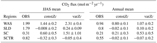
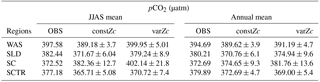
Table 3 JJAS mean and the climatological annual mean of export production from satellite-derived net primary production data, constZc and varZc simulations. Units are g C m⁻² yr⁻¹.

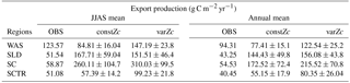
Table 4 Model-derived values for new production. Units are g C m⁻² yr⁻¹.

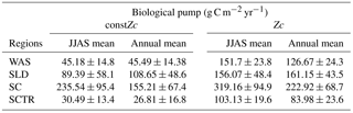
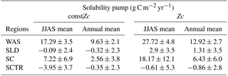
The impact of varZc in the biological and solubility pumps is computed as per Louanchi et al. (1996, see Appendix A). The varZc parameterisation strengthens the biological as well as the solubility pump in the model, thereby modifying the phosphate profiles and achieving a seasonal balance in export versus new production (Fig. 9a). During the monsoon period, the varZc simulation increases the strengths of the solubility and biological pumps by 10.43 ± 1.3 and 106.52 ± 9 g C m⁻² yr⁻¹, respectively (see Tables 5 and 6). Similarly, the annual mean strength of solubility pump and the biological pump are increased by 3.29 ± 0.6 and 81.18 ± 9.92 g C m⁻² yr⁻¹. This supports the fact that the varZc parameterisation basically modifies the biological and solubility pumps in the model simulation and thereby improves the seasonal cycle of CO₂ flux and pCO₂.

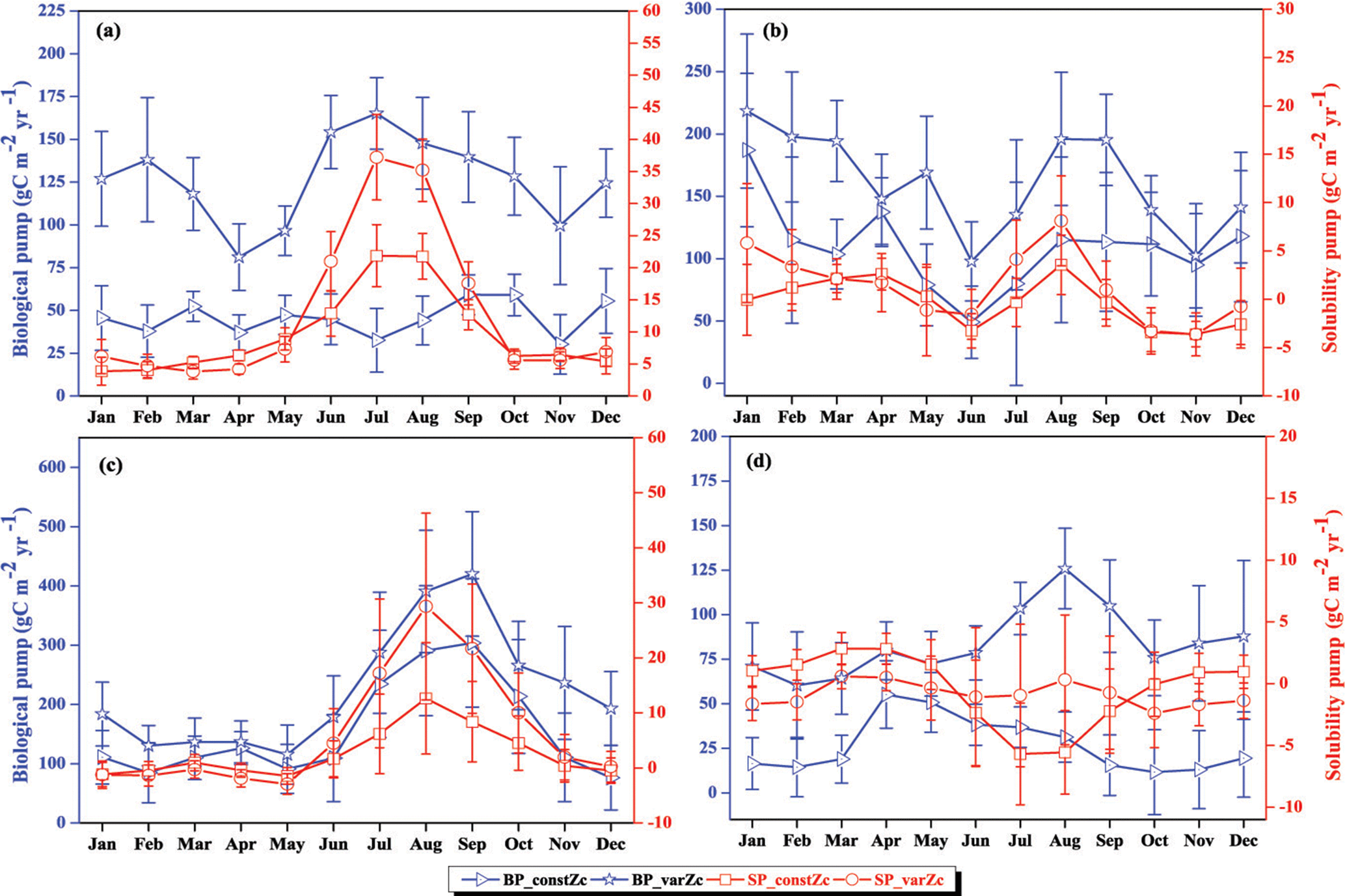
Figure 9 The strength of the biological pump (BP, blue lines) and solubility pump (SP, red lines) from constZc and varZc simulations for (a) WAS (b) SLD (c) SC and (d) SCTR. The left axis shows the biological pump and the right axis shows the solubility pump. Error bar shows standard deviations of individual months over the years 1990–2010. Units are g C m⁻² yr⁻¹.

3.3 Sri Lanka Dome (SLD)

The seasonal variation in Zc for the SLD has a similar pattern to that of WAS. Zc deepens to its maximum during March to 45.23 ± 0.3 m and reaches its minimum during the following monsoon period at 30.79 ± 1.5 m (Fig. 5). The similarities of varZc between the WAS and SLD indicate that they both are under similar cycles of solar influx and biological production. The SLD Chl a dominates only up to July (Vinayachandran et al., 2004), which explains why production with varZc increases earlier compared to WAS, which occurs during ASO.

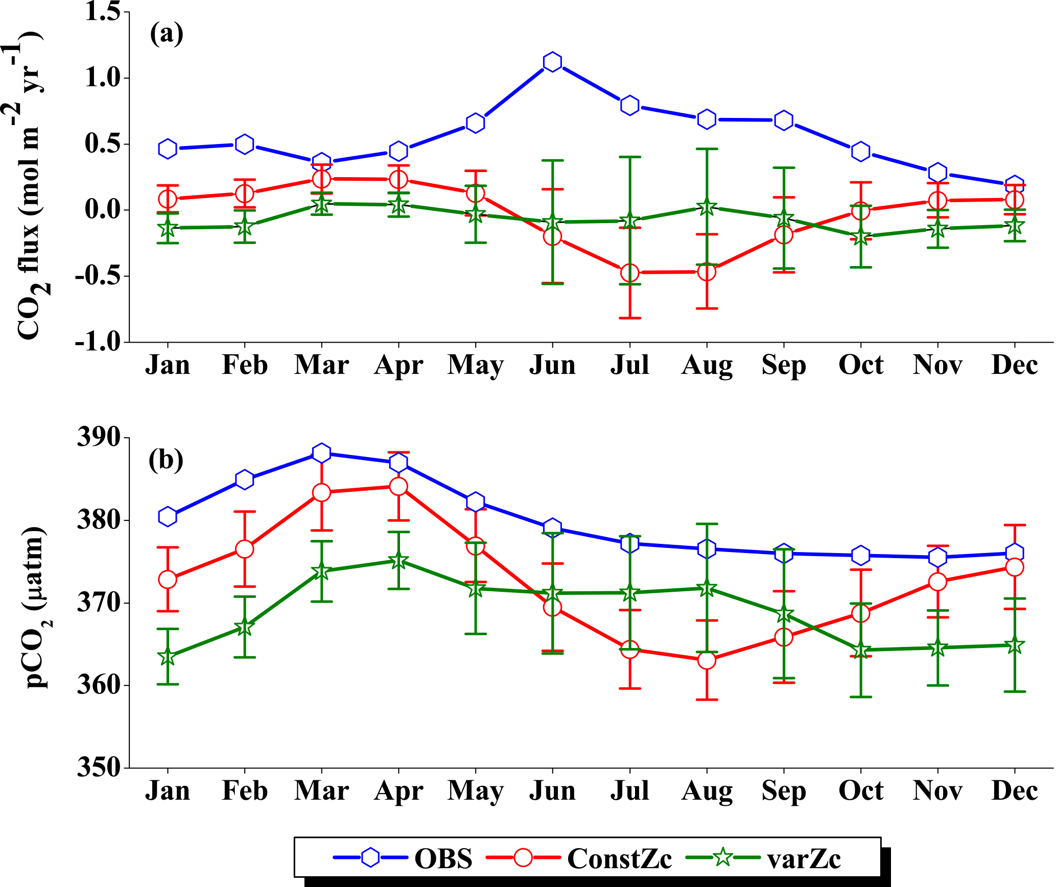
The seasonality in CO₂ flux and pCO₂ were compared with the Takahashi et al. (2009) observations (Fig. 10). varZc results in a slight improvement in CO₂ flux when compared with constZc (Fig. 10a). However, both constZc and varZc simulations underestimate the magnitude of CO₂ flux when compared with the observations. The seasonal mean CO₂ flux during the monsoon period is 1.79 mol m⁻² yr⁻¹ from the observations, which means the SLD region is a source of CO₂. But the mean values of constZc and varZc simulations yield flux values of −0.008 ± 0.2 and 0.24 ± 0.2 mol m⁻² yr⁻¹. The constZc simulation misrepresents the SLD region as a sink of CO₂ during the monsoon period, which is the opposite of the observations. The varZc simulation corrects this misrepresentation to a source albeit at a smaller magnitude by 0.24 ± 0.09 mol m⁻² yr⁻¹ for the monsoon period. Compared to the observations, the varZc case underestimates the magnitude of JJAS mean by 1.55 mol m⁻² yr⁻¹.

The annual mean CO₂ fluxes for constZc and varZc simulations are −0.02 ± 0.1 and 0.10 ± 0.2 mol m⁻² yr⁻¹. The varZc parameterisation leads to an improvement of 0.13 ± 0.1 mol m⁻² yr⁻¹ in the annual mean CO₂ flux when compared with constZc simulation. The observational annual mean of CO₂ flux is 0.80 mol m⁻² yr⁻¹, which is highly underestimated by both simulations. This indicates a regulation of biological production of the region by varZc, which makes this region a source of CO₂ during the monsoon. The role of the solubility pump may also be underestimated due to the biases in the physical drivers and the lack of mesoscale eddy activities in these simulations (Prasanna Kumar et al., 2002; Valsala and Murtugudde, 2015).

Table 5 Biological pump impact over DIC in the model due to constZc and varZc simulations for JJAS and annual mean.

Table 6 Same as Table 5, but for solubility pump.

The seasonality of pCO₂ (Fig. 10b), especially in the monsoon period, is significantly improved. The mean pCO₂ during the monsoon season from observations over the SLD region is 382.44 µatm. The seasonal mean pCO₂ during the monsoon period for constZc and varZc simulations are 371.67 ± 6.04 and 379.24 ± 8.9 µatm, respectively. The annual mean pCO₂ from observations, constZc and varZc simulations are 380.21, 370.76 ± 6.1 and 374.94 ± 9.6 µatm. varZc simulations improve the JJAS mean pCO₂ by 7.56 ± 2.8 µatm and the annual mean pCO₂ by 4.18 ± 3.5 µatm, which is reflected in CO₂ flux as well. This is likely due to the impact of a new biological parameterisation in capturing the episodic upwelling in the SLD region, which is further investigated by looking at its biological production.

Figure 10 Same as Fig. (6), but for SLD.

Figure 11 Same as Fig. (7), but for SLD.

Figure 12 Same as Fig. (6), but for SC.

Figure 13 Same as Fig. (7), but for SC.

Figure 14 Same as Fig. (6), but for SCTR.

Figure 15 Same as Fig. (7), but for SCTR.

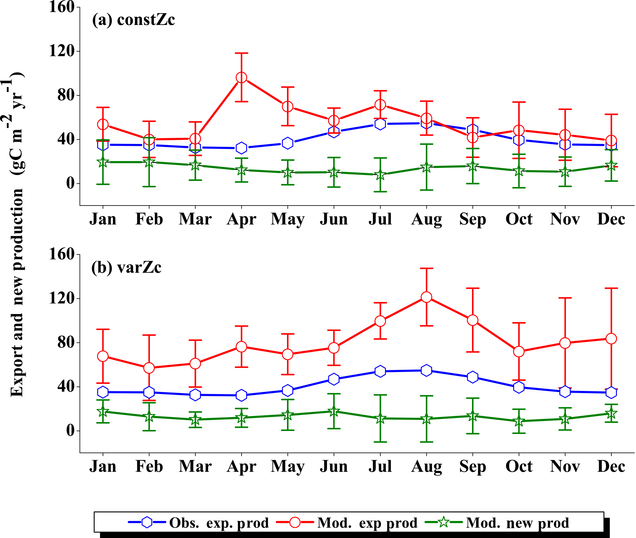
The SLD biological production is highly exaggerated by the model for both constZc and varZc simulations (Fig. 11a, b). The seasonal mean biological export for the monsoon period is 51.54 g C m⁻² yr⁻¹ as per satellite-derived estimates. However, the constZc and varZc simulations overestimate it at 167.71 ± 59.04 and 151.51 ± 46.4 g C m⁻² yr⁻¹, respectively. This exaggerated export is visible in climatological annual means where for constZc and varZc simulations they are 144.43 ± 49.8 and 156.08 ± 43.8 g C m⁻² yr⁻¹.

For the constZc simulation, new production is overestimated from March to October when compared to the observations and the second peak is observed in November (Fig. 11a). But the overestimate in new production with varZc is observed only during the JJAS period by an amount of 26.23 g C m⁻² yr⁻¹. For the SLD region, the varZc parameterisation overestimates the export production but minimizes the excess new production, especially in the monsoon period, by 64.15 ± 36.4 g C m⁻² yr⁻¹. This indicates that the varZc parameterisation is somewhat successful in capturing the upwelling episode during the monsoon over the SLD. All values are summarised in Tables 1 to 4.

The solubility and biological pumps are modified by the varZc parameterisation significantly when compared with the constZc simulation (Fig. 9b). Over the monsoon period, the strengths of the solubility and biological pumps are improved by 2.81 ± 1.1 and 66.68 ± 9.7 g C m⁻² yr⁻¹. Similarly, the annual mean strength of solubility and biological pump are increased by 0.99 ± 1.2 and 52.5 ± 5.1 g C m⁻² yr⁻¹. All values are provided in Tables 5 and 6.

3.4 Sumatra coast (SC)

The seasonal variation in Zc over the SC region lies between 40 and 46 m (Fig. 5). The seasonal maximum occurs during JFM, especially in March with a depth of 45.5 m. During the monsoon period, Zc shoals slightly with a minimum of 41.1 m in July. The variation in Zc is relatively small compared to the other regions, which is consistent with its relatively low production throughout the year.

The seasonality of CO₂ flux and pCO₂ captured by constZc and varZc simulations is shown in Fig. 12a, b. The varZc simulations overestimate both CO₂ flux and pCO_2,, especially during the monsoon. It is found that the constZc simulation is better compared to the varZc simulation. The varZc simulation overestimates the seasonal mean CO₂ flux and pCO₂ by 1.19 mol m⁻² yr⁻¹ and 29.61 µatm, respectively, compared to the observations (Table 1). However, constZc produces a better estimate compared with the observations for CO₂ flux and pCO₂. The constZc simulation also delivers a better annual mean than varZc (Tables 1, 2). The annual mean bias in constZc and varZc simulations for CO₂ flux is −0.0033 and 0.31 mol m⁻² yr⁻¹. Similarly, pCO₂ biases are 1.95 and 9.07 µatm for constZc and varZc simulations.

Biological production simulated by the model along SC explains the overestimation of CO₂ flux and pCO₂ (Fig. 13). Both constZc and varZc simulations greatly overestimate export production in the model. However, a small enhancement in the new production during JJAS in the constZc case is an indicator of upwelling episodes. The seasonal means of new production during the monsoon from constZc and varZc are 63.64 ± 30.9 and 78.11 ± 29.1 g C m⁻² yr⁻¹ (Table 4). The seasonal mean export production during the monsoon from the observations is 58.87 g C m⁻² yr⁻¹ (Table 3). The constZc simulation represents better new production, which is seen as a relatively small exaggeration of CO₂ flux and pCO₂. The biological response of SC is found to be better with constZc which is in contradiction to a general improvement found with varZc in the other regions examined here. Such discrepancies over the SC could be due to the effect of Indonesian throughflow (Bates et al., 2006), which is not completely resolved in the model due to coarse spatial resolution (also see Valsala and Maksyutov, 2010a).

The overestimation of export production by varZc simulation is also evident by the increase in strength of the biological and solubility pumps (Fig. 9c). The annual mean and JJAS mean DIC increases in the production zone due to the biological pump are 67.21 ± 1.3 and 83.62 ± 0.5 g C m⁻² yr⁻¹. Similarly the increases in DIC due to the effect of the solubility pump during the JJAS period and over the year are 10.95 ± 5.2 and 3.87 ± 2.2 g C m⁻² yr⁻¹ (see Tables 5 and 6).

3.5 Seychelles–Chagos thermocline ridge (SCTR)

The SCTR is a unique open-ocean upwelling region with prominent variability in air–sea interactions (Xie et al., 2002). Wind-driven mixing and upwelling of subsurface nutrient-rich water play a major role in the biological production of this region (Dilmahamod et al., 2016). The seasonal cycle in Zc is shown in Fig. 5. The maximum Zc occurs in November at about 44.94 m and the minimum at 33.2 m in July. The shoaling of Zc during the monsoon period shows that the biological parameterisation captures the response to upwelling over this region.

The seasonality of CO₂ flux and pCO₂ are shown in Fig. 14. The Takahashi observations of CO₂ flux show a peak in June with outgassing of CO₂ during the upwelling episodes. However, both constZc and varZc simulations underestimate this variability. The seasonality of CO₂ flux in varZc shows a significant improvement when compared to the constZc simulation, but is underestimated when compared to the observations. The seasonal mean CO₂ fluxes during the monsoon from the observations, constZc and varZc simulations are 0.82, −0.32 ± 0.3 and −0.05 ± 0.4 mol m⁻² yr⁻¹, respectively. This represents a reduction in the seasonal mean sink of the CO₂ flux in the SCTR region during the monsoon by 0.27 ± 0.1 mol m⁻² yr⁻¹, bringing it closer to a source region (see Table 1 for details).

The improved CO₂ flux is also supported by the seasonal cycle in pCO₂. Based on the observations, the seasonal mean of pCO₂ with constZc during JJAS is underestimated by 11.47 µatm, varZc simulation underestimates it by 6.45 µatm. So, it is evident that the varZc simulation captures the upwelling episodes better, marked by a larger pCO₂ during the JJAS period. However, the magnitude of pCO₂ is still underestimated compared to the observations (Table 2).

Figure 15 shows the biological production of constZc and varZc simulations for SCTR. It is clear that both simulations overestimate the export production and underestimate the new production. The JJAS mean export production from the observations, constZc and varZc are 51.08, 57.39 ± 14.2 and 99.23 ± 29.8 g C m⁻² yr⁻¹. The varZc simulations exaggerate the model export production by 48.14 g C m⁻² yr⁻¹. The varZc simulation improves the JJAS mean new production by 1.14 ± 2.2 g C m⁻² yr⁻¹ (Table 4). The DIC variations due to the biological pump over the monsoon period and the annual mean also correspond to the exaggerated export production. During the monsoon period, the varZc simulation strengthens the biological and solubility pumps by 72.64 ± 6.2 and −4.56 ± 1.6 g C m⁻² yr⁻¹ when compared to the constZc simulation (Fig. 9d). This is also reflected in the annual mean DIC variations due to the biological and solubility pump effects (see Tables 5 and 6). This slight improvement in the model new production, especially during the monsoon period, signals that the varZc better captures the upwelling over SCTR. Considering the annual mean values of model export and new production, the constZc simulation is reasonably faithful to the observations.

The underestimation of CO₂ and pCO₂, as well as the exaggeration of model export production and a slight overestimation in the model new production, may be due to two factors: (1) SCTR is a strongly coupled region with remote forcing of the mixed layer – thermocline interactions (Zhou et al., 2008) which can affect the seasonality in biological production that the model may not be resolving reasonably, (2) the bias associated with physical drivers, especially wind stress, may underestimate the CO₂ flux as well as biological production. A similar overestimation of biological production was also reported in a coupled biophysical model (Dilmahamod et al., 2016).

Tables 1–4 shows the entire summary of seasonal and annual mean CO₂ flux, pCO₂ and biological production reported in Sect. 3.

4 Summary and conclusions

A spatially and temporally varying Zc parameterisation as a function of solar radiation and Chl a is implemented in the biological pump model of OCMIP-II for a detailed analysis of biological fluxes in the upwelling zones of the Indian Ocean. The varZc parameterisation improves the seasonality of model CO₂ flux and pCO₂ variability, especially during the monsoon period. A significant improvement is observed in WAS where the monsoon wind-driven upwelling dominates biological production. The magnitude of the CO₂ flux matches with the observations, especially in July when monsoon winds are at their peak. The monsoon triggers upwelling in the SLD as well, which acts as a source of CO₂ to the atmosphere. The seasonal and annual mean are underestimated with constZc, and the SLD is reduced to a sink of CO₂ flux. The varZc simulation modifies the seasonal and annual mean of the CO₂ flux of the SLD and depict it as a source of CO₂, especially during the monsoon, but the magnitude is still underestimated compared to the Takahashi et al. (2009) observations. The SCTR variability is underestimated by both constZc and varZc simulations, portraying it as a CO₂ sink region, whereas observations over the monsoon period indicate that the thermocline ridge driven by the open-ocean wind-stress curl is, in fact, an oceanic source of CO₂. However, the varZc simulation reduces the magnitude of the sink in this region by bringing it relatively close to the observations.

VarZc biological parameterisation strengthens the export and new productions in the model, which allows it to represent a better seasonal cycle of CO₂ flux and pCO₂ over the study regions. The WAS export production is remarkably improved by 62.37 ± 7.8 g C m⁻² yr⁻¹ compared to constZc. This supports our conclusion that the varZc parameterisation increases the strength of biological export in the model. Over the SLD, the JJAS seasonal mean export and new production are underestimated in varZc compared to constZc simulations, but the annual mean export production is improved. Export production at SC and SCTR are highly exaggerated and there is hardly any improvement in the new production, with a variable Zc especially over the monsoon period. The inability of varZc parameterisation to improve the seasonality of SC and SCTR may be due to the interannual variability of biological production associated with the Indonesian throughflow and remote forcing of the mixed-layer thermocline interactions and the effect of biases in the wind stress data used as a physical driver in the model.

Sensitivity experiments carried out by prescribing annual mean currents or temperatures over selected subdomains reveal that the varZc retains the seasonality of carbon fluxes, pCO₂ and export and new productions closer to the observations. This strongly supports our contention that varZc parameterisation improves export and new productions and it is also efficient in capturing upwelling episodes of the study regions. This points out the significant role of having a close balance in seasonal biological export and new production in models to capture the seasonality in the carbon cycle. This also confirms the role of biological and solubility pumps in producing the seasonality of the carbon cycle in the upwelling zones.

However, the underestimation of the seasonality of CO₂ flux over the SLD and overestimation over the SC as well as the SCTR are a cautionary flag for the study. This uncertainty poses an important scientific question as to whether the model biology over the SC and SCTR region is not resolving the seasonality in CO₂ flux and pCO₂ properly or whether the seasonality in the Zc is not able to fully capture the biological processes.

To address these questions we have used an inverse modelling approach (Bayesian inversion) in order to optimise the spatially and temporally varying Zc using surface pCO₂ as the observational constraint and computed the optimised biological production. The results will be reported elsewhere.

Appendix A

The time evolution equations of the model variables are given by

$$\begin{array}{}\text{(A1)}& {\displaystyle }& {\displaystyle \frac{d\left[{\mathrm{PO}}_{\mathrm{4}}\right]}{\mathrm{d}t}}=L\left(\left[{\mathrm{PO}}_{\mathrm{4}}\right]\right)+J_{{\mathrm{PO}}_{\mathrm{4}}}\text{(A2)}& {\displaystyle }& {\displaystyle \frac{d\left[\mathrm{DOP}\right]}{\mathrm{d}t}}=L\left(\left[\mathrm{DOP}\right]\right)+J_{\mathrm{DOP}}\text{(A3)}& {\displaystyle }& {\displaystyle \frac{d\mathrm{DIC}}{\mathrm{d}t}}=L\left(\left[\mathrm{DIC}\right]\right)+J_{\mathrm{DIC}}+J_g\mathrm{DIC}+J_v\mathrm{DIC}\text{(A4)}& {\displaystyle }& {\displaystyle \frac{d\left[\mathrm{ALK}\right]}{\mathrm{d}t}}=L\left(\left[\mathrm{ALK}\right]\right)+J_{\mathrm{ALK}}+J_v\mathrm{ALK},\end{array}$$

where L is the 3-D transport operator, which represents the effects of advection, diffusion and convection. Square brackets indicate the concentrations in mol m⁻³. $J_{{\mathrm{PO}}_{\mathrm{4}}}$, J_DOP, J_DIC and J_ALK are the biological source–sink terms, and J_vDIC and J_vALK are the virtual source–sink terms representing the changes in surface DIC and ALK due to evaporation and precipitation. J_gDIC is the source–sink term due to air–sea exchange of CO₂.

The following equations represent the biological processes in the model.

For Z < Zc

$$\begin{array}{}\text{(A5)}& {\displaystyle }& {\displaystyle }{J}_{\mathrm{prod}}={\displaystyle \frac{\mathrm{1}}{\mathit{\tau }}}\left(\left[{\mathrm{PO}}_{\mathrm{4}}\right]-\left[{\mathrm{PO}}_{\mathrm{4}}{}^{\ast }\right]\right),\left[{\mathrm{PO}}_{\mathrm{4}}\right]>\left[{\mathrm{PO}}_{\mathrm{4}}{}^{\ast }\right]\text{(A6)}& {\displaystyle }& {\displaystyle }{J}_{\mathrm{DOP}}=\mathit{\sigma }{J}_{\mathrm{prod}}-\mathit{\kappa }\left[\mathrm{DOP}\right]\text{(A7)}& {\displaystyle }& {\displaystyle }{J}_{\mathrm{PO}{}_{\mathrm{4}}}=-J_{\mathrm{prod}}+\mathit{\kappa }\left[\mathrm{DOP}\right]\text{(A8)}& {\displaystyle }& {\displaystyle }{J}_{\mathrm{ca}}=R{r}_{\mathrm{C}:\mathrm{P}}(\mathrm{1}-\mathit{\sigma })J_{\mathrm{prod}}\text{(A9)}& {\displaystyle }& {\displaystyle }{J}_{\mathrm{DIC}}=r_{\mathrm{C}:\mathrm{P}}{J}_{\mathrm{PO}{}_{\mathrm{4}}}+J_{\mathrm{ca}}\text{(A10)}& {\displaystyle }& {\displaystyle }{J}_{\mathrm{ALK}}=-r_{\mathrm{N}:\mathrm{P}}{J}_{\mathrm{PO}{}_{\mathrm{4}}}+\mathrm{2}{J}_{\mathrm{ca}}.\end{array}$$

For Z > Zc

$$\begin{array}{}\text{(A11)}& {\displaystyle }& {\displaystyle }{J}_{\mathrm{prod}}=\mathrm{0},\left[{\mathrm{PO}}_{\mathrm{4}}\right]\le \left[{\mathrm{PO}}_{\mathrm{4}}{}^{\ast }\right]\text{(A12)}& {\displaystyle }& {\displaystyle }{J}_{\mathrm{DOP}}=-\mathit{\kappa }\left[\mathrm{DOP}\right]\text{(A13)}& {\displaystyle }& {\displaystyle }{J}_{\mathrm{PO}{}_{\mathrm{4}}}=-{\displaystyle \frac{\partial F}{\partial Z}}+\mathit{\kappa }\left[\mathrm{DOP}\right]\text{(A14)}& {\displaystyle }& {\displaystyle }{F}_c=(\mathrm{1}-\mathit{\sigma })\underset{\mathrm{0}}{\overset{\mathit{\text{Zc}}}{\int }}{J}_{\mathrm{prod}}\mathrm{d}Z\text{(A15)}& {\displaystyle }& {\displaystyle }F\left(Z\right)=F_c({\displaystyle \frac{Z}{\mathit{\text{Zc}}}}{)}^{-a}\text{(A16)}& {\displaystyle }& {\displaystyle }{J}_{\mathrm{ca}}=-{\displaystyle \frac{\partial F_{\mathrm{Ca}}}{\partial Z}}\text{(A17)}& {\displaystyle }& {\displaystyle }{F}_{\mathrm{Ca}}=R{r}_{\mathrm{C}:\mathrm{P}}{F}_C{e}^{-(Z-\mathit{\text{Zc}})/d},\end{array}$$

where Z is the depth and Zc is the compensation depth in the model. J_prod and J_Ca represent the biogeochemical flows with respect to production and calcification. Within Zc, the production of organic phosphorous in the model J_prod is calculated using Eq. (A5). [PO₄] is the model phosphate concentration and [PO₄^∗] is observational phosphate. τ is the restoration timescale assumed to be 30 days. Whenever the model phosphate exceeds the observational phosphate, it allows production, below which the production is zero. The observational phosphate data were taken from the World Ocean Atlas (WOA; Garcia et al., 2014). It is assumed that a fixed fraction (σJ_prod) of phosphate uptake is converted into dissolved organic phosphorus (DOP), which is a source for J_DOP (Eq. A6). The phosphate not converted to DOP results in an instantaneous downward flux of particulate organic phosphorus at Zc (Eq. A14). The decrease of flux with depth due to remineralisation is shown by a power law relationship as in Eq. (A15). The values of the constants a, κ, σ are 0.9, 0.2 yr⁻¹ to 0.7 yr⁻¹, 0.67. The rate of production is used to explain the formation of calcium carbonate cycle in surface waters (Eq. A8) and its export is given by Eq. (A16), where R is the rain ratio, a constant molar ratio of exported particulate organic carbon to the exported calcium carbonate flux at Zc. The exponential decrease of calcium carbonate flux with scale depth d is given by Eq. (A17). The biological source or sink of dissolved inorganic carbon (DIC) and alkalinity (ALK) is explained through Eqs. (A9) and (A10). Where the value of rain ratio (R) is taken as 0.07, the Redfield ratio is $r_{\mathrm{C}:\mathrm{P}}=\mathrm{117}$, and $r_{\mathrm{N}:\mathrm{P}}=\mathrm{16}$ and scale depth d is chosen as 3500 m.

A1 Biological and solubility pump calculations

The biological effect on DIC is calculated from Louanchi et al. (1996). The tendency of DIC due to biomass production and calcite formation in the production zone is expressed below.

$$\begin{array}{}\text{(A18)}& {\displaystyle }{\left({\displaystyle \frac{\partial \mathrm{DIC}}{\partial t}}\right)}_b={\left({\displaystyle \frac{\partial {\mathrm{PO}}_{\mathrm{4}}}{\partial t}}\right)}_b\times R_{\mathrm{C}:\mathrm{P}}-J_{\mathrm{Ca}}\end{array}$$

The total tendency of DIC in the production zone is

$$\begin{array}{}\text{(A19)}& {\displaystyle }{\left({\displaystyle \frac{\partial \mathrm{DIC}}{\partial t}}\right)}_{\mathrm{total}}={\left({\displaystyle \frac{\partial DIC}{\partial t}}\right)}_{\mathrm{b}}+\underset{x}{\int }\underset{y}{\int }F\mathrm{d}x\mathrm{d}y,\end{array}$$

where ${\left(\frac{\partial \mathrm{DIC}}{\partial t}\right)}_{\mathrm{b}}$ is the evolution of DIC due to the impact of biology (i.e. biological pump). The first term on the right side of Eq. (A18) is the rate of change of phosphate resulting from photosynthesis and respiration in the model (i.e. $J_{\mathrm{PO}{}_{\mathrm{4}}}$ in this case) multiplied by the carbon-to-phosphorous Redfield ratio ($R_{\mathrm{C}:\mathrm{P}}=$ 117 : 1) and J_Ca represents the calcite formation in the model (see Eqs. A8 and A16). The solubility pump is calculated as the surface integral of the flux F (Louanchi et al., 1996).

Appendix B

In order to compare our model production of organic phosphorous to the curve of Ryther et al. (1956) we have merely scaled our total production to “relative photosynthesis”, which is, according to Ryther et al. (1956), an index between 0 and 1 indicating the strength of production estimated as P_l ∕ P_max. Here P_l is the photosynthesis at each intensity (of light) of different species and P_max is the maximum photosynthesis observed in the same control experiment. The curve between relative photosynthesis and light intensity shows the relation between photosynthetic activity and light in marine phytoplankton. Since our method relates biological production to a function of light (limitation) by Chl a attenuation, it is the best curve with which to cross-compare our results. In this case we scaled our total biological production within Zc to relative values between 0 and 1 by P_l ∕ P_max in which P_l is taken as the individual grid cell biological component of organic phosphorus production and P_max is the maximum production available in the domain at any given instant. All the grid points are quite similar to the curve of Ryther et al. (1956), as shown in Fig. 2.